Embed Size (px)
Citation preview

Assessment of Redundant Systems
with Imperfect Coverage
by means of Binary Decision Diagrams
Albert F. Myers
Northrop Grumman Corporation
1840 Century Park East
Los Angeles, California 90067-2199
USA
Antoine Rauzy
IML/CNRS,
163, avenue de Luminy,
13288 Marseille Cedex 09,
FRANCE
Abstract: In this article, we study the assessment of the reliability of redundant systems
with imperfect fault coverage. We term fault coverage the ability of a system to isolate
and correctly accommodate failures of redundant elements. For highly reliable systems,
such as avionic and space systems, fault coverage is in general imperfect and has a
significant impact on system reliability. We review here the different models of
imperfect fault coverage. We propose efficient algorithms to assess them separately (as
k-out-of-n selectors). We show how to implement these algorithms into a Binary
Decision Diagrams engine. Finally, we report experimental results on real life test cases
that show on the one hand the importance imperfect coverage and on the other hand the
efficiency of the proposed approach.
Keywords: Imperfect coverage of redundant systems, k-out-of-n systems, Binary
Decision Diagrams.
1. Introduction
Computer controlled systems used in life-critical applications often utilize redundancy to
meet the stringent levels of reliability required. An increasing interest in the development
of highly reliable systems has resulted in an extensive treatment of reliability models for
k–out–n systems in the literature. Only a much smaller portion of this literature,
however, addresses the modeling of imperfect fault coverage (IFC) for these redundant
systems [AM99, CAK02, ADM99, DDP95, Dug89, DT89, Mye06, Tri02]. The proper
operation of all redundant systems is clearly dependent on the system's ability to detect,
isolate and correctly accommodate failures of the redundant elements. The probability of
correctly accomplishing these tasks is termed coverage. For highly reliable systems, even
for very high values approaching unity, coverage has a significant effect on system
reliability. As a result, appropriate modeling of the effects of coverage is critical to the
design of these systems, particularly for those whose operation is life critical.
The redundancy management (RM) process of a redundant system is responsible for the
following tasks; (1) the detection of faults among the system's elements, (2) the isolation
of a fault to a particular element, and (3) the reconfiguration of the system in such a way
as to assure the system's proper operation subsequent to a redundant element failure. For
systems in which the RM tasks are accomplished under computer control, this process
can seldom, perhaps never, be done with perfect certainty. There are two main
techniques used as a primary basis for the implementation of a system's RM function; (1)
the RM tasks are accomplished using a diagnostic process that is associated with each of
the individual redundant elements, this typically takes advantage of a built in test
capability (BIT) incorporated within the redundant element, or (2) the RM function may
take advantage of some version of mid-value-select voting when there are at least 3
operational elements within the system's set of redundant elements of a given type.
Systems utilizing these two RM techniques require different approaches for the modeling
of system reliability. Those utilizing the first type of RM (BIT) are modeled using what
we term element level coverage (ELC) while the second RM approach (voting) are
modeled using a fault level coverage (FLC) model. For all IFC systems (whether ELC or
FLC) an "uncovered" failure results in system failure even though sufficient redundancy
may still exist.
In this article, we propose efficient table based algorithms for k-out-of-n:F systems
subject to IFC for both ELC and FLC systems. These algorithms are based on a recursive
decomposition inspired from those used for general k-out-of-n:F systems proposed in
[DR01]. We show that both algorithms have a O(n.k) time complexity. With such a low
complexity, virtually any real life system can be assessed within few seconds. The ELC
functions presented in this paper produce results identical to those computed using the
SEA algorithm [AM99]. Similarly, presented FLC functions produce the same results as
the Ral procedure presented in [Mye06]. In both cases however, the functions presented
here achieve a much better complexity.
Voters are in general embedded into broader systems whose failures are conveniently
modeled by means of fault trees. It is therefore of interest to be able to encode ELC and
FLC models by means of the usual fault tree gates. Although the recursive
decomposition we propose makes such an encoding possible, we adopt here a slightly
different approach. Namely, we propose to define new types of gates, one for each IFC
model. We show that the table based algorithms can be adapted to the construction of
Binary Decision Diagrams (BDD). Since BDD have proved to be the most efficient
technology to assess fault trees, we end up with a powerful tool to assess general systems
with IFC components.
The remainder of this article is organized as follows. Section 2 presents a taxonomy for
these classes of imperfect fault coverage systems. Section 3 proposes the table based
algorithms to assess these models. It reports also results of small experiments that show
the efficiency of these algorithms as well as the impact of the coverage on k-out-of-n:F
systems. Section 4 proposes a BDD based implementation of the models. Finally,
section 5 reports some results on a realistic test case.

2. Imperfect Fault Coverage Models
In this section, we shall consider the different IFC models, i.e. k-out-of-n:F systems using
ELC, FLC or OLC models. Recall that a k-out-of-n:F system is a system with n
redundant, not necessarily identical, components that fails when at least k out of the n
components have failed. The taxonomy presented hereafter is mainly borrowed to from
Myers work [Mye06].
2.1. ELC Systems
A ELC system is a k-out-of-n system where each component ei, i=1,…,n, is associated
with a coverage value ci (i.e. a probability of individual fault coverage). The system is
failed if either one of the ei’s is failed uncovered or if at least k of the ei’s are failed
(uncovered).
ELC is appropriate in the circumstance where the RM selection among the redundant
elements is made on the basis of a self–diagnostic capability of the individual elements,
i.e., the redundant elements have not only their primary output but also a status signal
indicating the health of the element. If ELC is used to model the reliability of a system
whose redundant elements utilize BIT then the product of the probability that the BIT
will correctly identify the failure of its associated element and the reliability of the BIT
system itself can be utilized as the coverage value for the associated element. The
achievable level of ELC will, in actual systems, depend on the time scale required by the
RM process. For systems in which the RM process can be run with a periodicity
measured on the order of several seconds or minutes (or longer) BIT reliability, and as a
result ELC coverage level, may be in excess of 99%, depending on the nature of the
element's BIT. However, for systems for which the RM task must be performed multiple
times per second, such as required for aircraft digital flight control systems, element BIT
generally cannot be done with a confidence greater than 90 to 99%. These differences in
BIT confidence are the result of the fact that exhaustive BIT is often not possible in very
short times, i.e., given enough time the BIT can test a greater fraction of its possible
failure modes. Systems utilizing RM architectures based on ELC are generally not
capable of meeting extremely stringent reliability requirements such as those required for

aircraft flight control systems. This is because the level of achievable coverage (generally
99% or less) severely limits the level of reliability achievable through the use of
redundancy.
2.2. FLC Systems
A FLC system is a k-out-of-n system that organizes a vote amongst components e1, e2…
en. The first failure has a probability c1 to be covered, the second one a probability c2, and
so on up to k-1 (the k-th failure will fail the system whether it is covered or not). Again,
the system is failed if either one of the ei’s is failed uncovered or if at least k of the ei’s
are failed (uncovered).
FLC is appropriate for modeling systems in which the fault detection and reconfiguration
RM tasks vary between initial and subsequent failures. For a system in which the fault
detection and reconfiguration logic is based on the comparison of the outputs, i.e., voting,
of the redundant elements are candidates for FLC modeling. A system with three or more
redundant elements can be designed to assure extremely high levels of coverage so long
as a mid-value-select (MVS) voting strategy can be applied. However, selection from
among the last two remaining elements, whose outputs do not agree by an amount in
excess of some predetermined fault detection threshold, cannot be done with the same
high level of coverage. Note that this lower level of coverage is not due to the inability of
detecting the fault but, rather, the ability of determining which of the two disagreeing
elements is the failed one. RM for this one-on-one case is typically accomplished by
using BIT (as done for ELC systems) along with other heuristics based on the nature of
the element. Thus for initial faults (those occurring when the redundant set still has 3 or
more elements of a given type) are subject to FLC very nearly unity, while, after the
system has failed down to a one-on-one configuration, the coverage will be no better than
that typically associated with ELC systems. For FLC systems, coverage for the initial
faults are very close to unity and only the one-on-one fault has a coverage level typical of
an ELC system, and, as a result, FLC systems can be designed to achieve much lower
levels of failure probability. For this reason most digital aircraft flight control systems
(typically designed to have a probability of failure on the order of 10-7 to 10
-9 per flight
hour) are designed as FLC systems.
2.3. OLC Systems
Since the coverage levels for initial faults in FLC systems can be very close to unity they
can frequently be modeled with sufficient accuracy by assuming that these initial
coverage values are in fact unity. This simplification can significantly reduce the
complexity of the system reliability calculations. A model using this approximation for
one–on–one level coverage is given the term OLC.
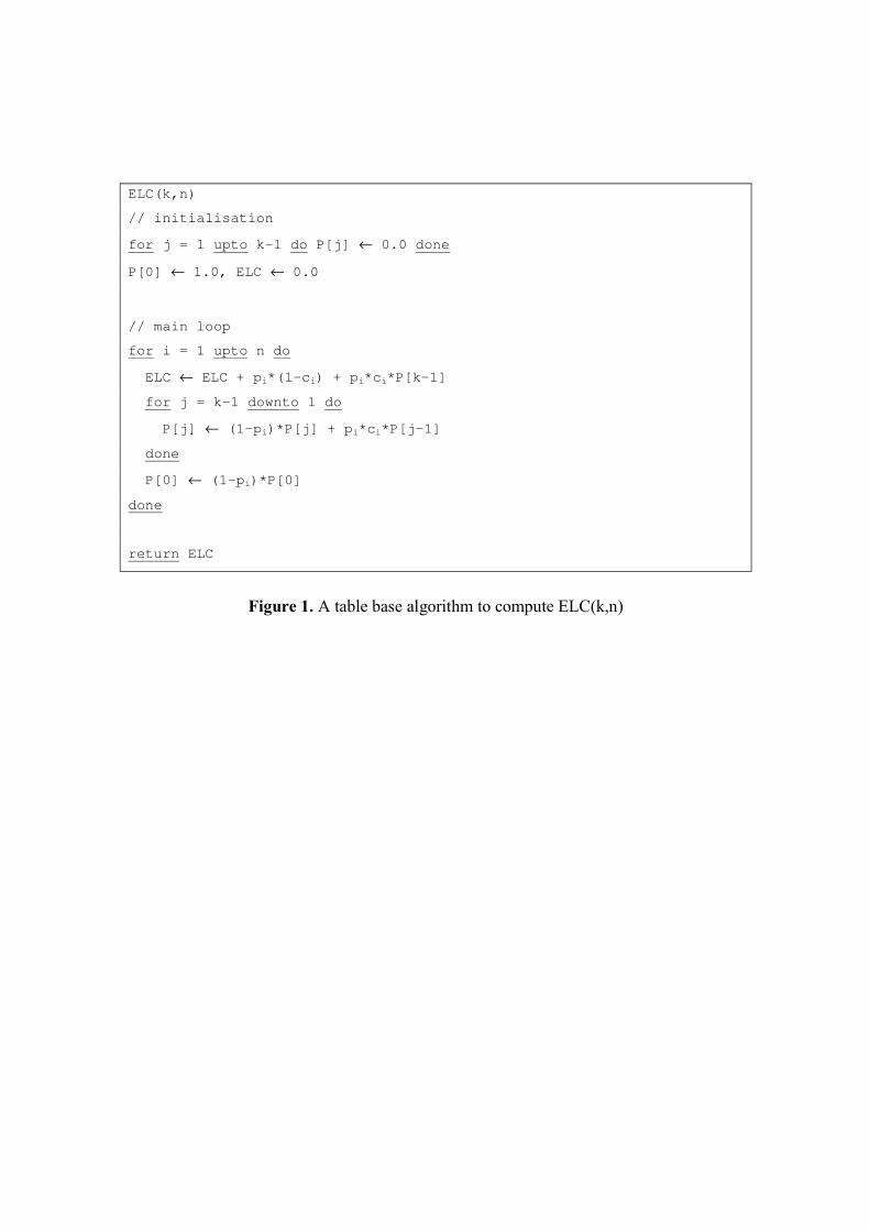
3. Table based Algorithms for ELC and FLC models
3.1. ELC Systems
Consider a k-out-of-n:F ELC system and the situation at mission time t. Let us denote by
pi i=1,…,n the probability that the i-th component fails between 0 and t. Let us denote by
ci i=1,…,n the probability that the failure of the i-th component is covered. Finally, let us
denote by ELC(k,n) the probability that the k-out-of-n:F ELC system is failed at t.
Now consider the n-th component. There are three possibilities.
• This component did not fail. In that case, the remainder of the components
worked as an ELC k-out-of-(n-1) system.
• This component failed covered. In that case, the remainder of the components
worked as an ELC (k-1)-out-of-(n-1) system.
• This component failed uncovered. In that case, the system failed.
So, we can write the following equations for ELC(k,n).
ELC(k,n) = (1-pn).ELC(k,n-1) + pn.cn.ELC(k-1,n-1) + pn.(1-cn)
Terminal cases are the following.
ELC(0,n) = 1 n>0
ELC(k,0) = 0 k>0

It is easy to derive an algorithm from the above recursive equation. However, one can
verify that this algorithm has a complexity in
Ο ∑
=
k
i i
n
1
, which is indeed unacceptable
for large values of n (and k). Fortunately, it is possible to memorize intermediate results,
similarly to what proposed by Dutuit and Rauzy in reference [DR01]. The idea is to use a
table P to store the probability that 0, 1…, k-1 failed components. A loop iterates over
the n components and the probability of failure is accumulated into a variable ELC. So,
at the i-th step, we consider separately the cases where 0, 1, 2…, k components amongst
the i-1 first components are failed. The algorithm is given Figure 1. It is easy to verify
that the complexity of this algorithm is in O(n.k).
3.2. FLC Systems
The recursive principle that governs FLC systems is very similar to equation (1). Let us
define now cj (j=1,…,n) has the conditional probability that at least j components are
failed covered given that at least j components are failed and at least j-1 components are
failed covered.
To make things a bit more concrete, consider a 2-out-of-4:F system. Consider the
configuration C in which component 1 and 3 are failed and 2 and 4 are working at time t.
The intrinsic probability of this configuration is as follows.
p(C) = p1.(1-p2).p3.(1-p4)
Now, we have the following case study:
• The probability that neither component 1 nor component 3 is covered is (1-c1).
• The probability that exactly one of these two components is covered is c1.(1-c2)
• Finally, the probability that both components are covered is c1.c2.
So, the probability that the system is in configuration C and is working is as follows.
p(C and working) = p(C).c1.c2
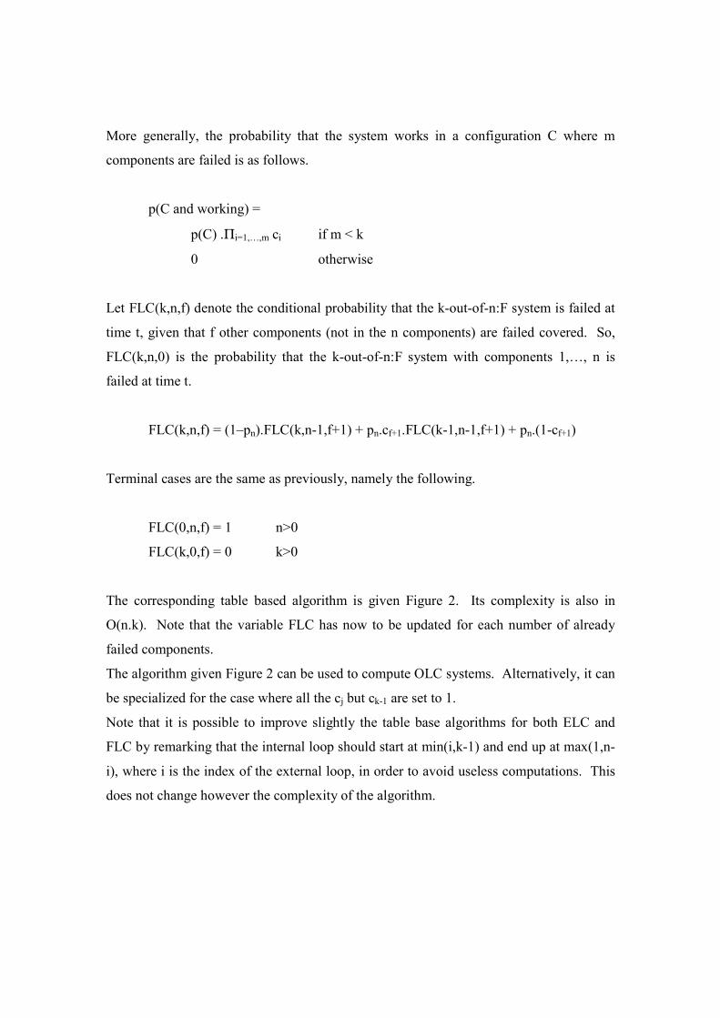
More generally, the probability that the system works in a configuration C where m
components are failed is as follows.
p(C and working) =
p(C) .Πi=1,…,m ci if m < k
0 otherwise
Let FLC(k,n,f) denote the conditional probability that the k-out-of-n:F system is failed at
time t, given that f other components (not in the n components) are failed covered. So,
FLC(k,n,0) is the probability that the k-out-of-n:F system with components 1,…, n is
failed at time t.
FLC(k,n,f) = (1–pn).FLC(k,n-1,f+1) + pn.cf+1.FLC(k-1,n-1,f+1) + pn.(1-cf+1)
Terminal cases are the same as previously, namely the following.
FLC(0,n,f) = 1 n>0
FLC(k,0,f) = 0 k>0
The corresponding table based algorithm is given Figure 2. Its complexity is also in
O(n.k). Note that the variable FLC has now to be updated for each number of already
failed components.
The algorithm given Figure 2 can be used to compute OLC systems. Alternatively, it can
be specialized for the case where all the cj but ck-1 are set to 1.
Note that it is possible to improve slightly the table base algorithms for both ELC and
FLC by remarking that the internal loop should start at min(i,k-1) and end up at max(1,n-
i), where i is the index of the external loop, in order to avoid useless computations. This
does not change however the complexity of the algorithm.
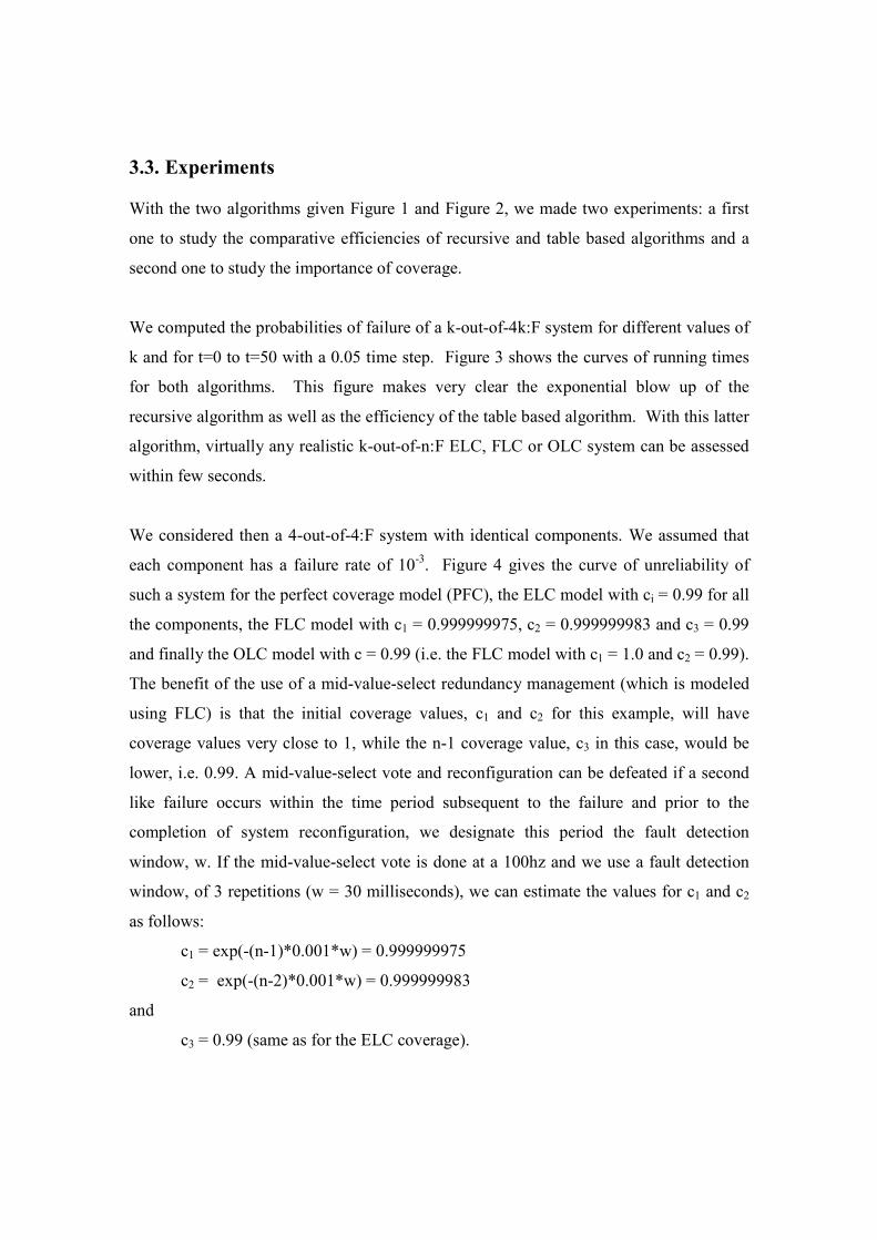
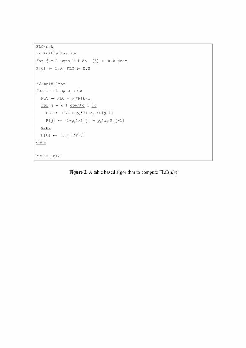
3.3. Experiments
With the two algorithms given Figure 1 and Figure 2, we made two experiments: a first
one to study the comparative efficiencies of recursive and table based algorithms and a
second one to study the importance of coverage.
We computed the probabilities of failure of a k-out-of-4k:F system for different values of
k and for t=0 to t=50 with a 0.05 time step. Figure 3 shows the curves of running times
for both algorithms. This figure makes very clear the exponential blow up of the
recursive algorithm as well as the efficiency of the table based algorithm. With this latter
algorithm, virtually any realistic k-out-of-n:F ELC, FLC or OLC system can be assessed
within few seconds.
We considered then a 4-out-of-4:F system with identical components. We assumed that
each component has a failure rate of 10-3. Figure 4 gives the curve of unreliability of
such a system for the perfect coverage model (PFC), the ELC model with ci = 0.99 for all
the components, the FLC model with c1 = 0.999999975, c2 = 0.999999983 and c3 = 0.99
and finally the OLC model with c = 0.99 (i.e. the FLC model with c1 = 1.0 and c2 = 0.99).
The benefit of the use of a mid-value-select redundancy management (which is modeled
using FLC) is that the initial coverage values, c1 and c2 for this example, will have
coverage values very close to 1, while the n-1 coverage value, c3 in this case, would be
lower, i.e. 0.99. A mid-value-select vote and reconfiguration can be defeated if a second
like failure occurs within the time period subsequent to the failure and prior to the
completion of system reconfiguration, we designate this period the fault detection
window, w. If the mid-value-select vote is done at a 100hz and we use a fault detection
window, of 3 repetitions (w = 30 milliseconds), we can estimate the values for c1 and c2
as follows:
c1 = exp(-(n-1)*0.001*w) = 0.999999975
c2 = exp(-(n-2)*0.001*w) = 0.999999983
and
c3 = 0.99 (same as for the ELC coverage).

With these values for FLC coverage, we can make a fair comparison with the ELC
results. Figure 4 shows clearly that the coverage cannot be ignored, even for very high
values of the coverage probability. The figure also shows that for mission times > 4, OLC
provides an excellent approximation to the more rigorous FLC result.
Note that it is not possible to simulate the impact of imperfect coverage by increasing the
failure rates of individual components. To illustrate that point, we considered the same 4-
out-of-4:F system under perfect coverage, but with failure rates set to 10-3, 2 10-3, 3 10-3,
4 10-3 and 5 10
-3. The resulting curve is shown Figure 5. This figure shows clearly that
the shape of the curve of perfect and imperfect coverage models are by no means the
same.
4. Binary Decision Diagrams Implementation
Bryant’s Binary Decision Diagrams [Bry86], BDD for short, are now a well-known and
widely used technique [Bry92]. In this section, we give first an encoding of PFC and IFC
models by means of classical fault tree gates. Then, we recall briefly the basics of this
technique. Finally, we show how to use it to implement PFC, ELC, OLC and FLC
models.
4.1. Encoding PFC and IFC models into fault trees
Consider first a k-out-of-n:F PFC system. Assume that the failures of each component ei
are described by means of a (sub)-fault tree rooted by the gate (or the basic event) ei (for
the sake of the simplicity, we keep the same name for the component and the top event of
the corresponding fault tree). Note that fault trees rooted by the ei’s may share gates and
basic events. The first idea is to associate a basic event with each coverage parameter,
i.e. a basic event ci, i=1,..,n, is associated to the component ei in the case of ELC models,
a basic event ci, i=1,…,k-1, is associated to each failure level in the case of FLC models
and a unique basic event c is associated with the k-1-th failure coverage in the case of
OLC models. The recursive decomposition may be encoded by means of gates AND, OR

and NOT and the Boolean constants TRUE and FALSE. For instance, the formula
ELC(n,k) associated a k-out-of-n ELC system is defined recursively as follows.
ELC(k,n) =
( NOT(en) AND ELC(k,n-1) )
OR ( en AND cn AND ELC(k-1,n-1) )
OR ( en AND NOT(cn) )
Terminal cases are the following.
ELC(0,n) = TRUE n>0
ELC(k,0) = FALSE k>0
The derivation of the formulae for PFC, FLC and OLC models follows the same line.
4.2. Binary Decision Diagrams
The Binary Decision Diagram of a formula is a compact encoding of the truth table of
this formula. From a BDD, it is possible to perform efficiently all of the probabilistic
quantifications (top event probability, importance factors…). The BDD representation is
based on the Shannon decomposition: Let F be a Boolean formula that depends on the
variable v, then
][.][. 01 ←+←= vFvvFvF
By choosing a total order over the variables and applying recursively the Shannon
decomposition, the truth table of any formula can be graphically represented as a binary
tree. The nodes are labelled with variables and have two out edges (a then-out edge,
pointing to the node that encodes F[v←1], and an else-out edge, pointing to the node that
encodes F[v←0]). The leaves are labelled with either 0 or 1. The value of the formula for
a given variable assignment is obtained by descending along the corresponding branch of
the tree. The Shannon tree for the formula F ab ac= + and the lexicographic order is
pictured Figure 7 (dashed lines represent else-out edges).
Indeed such a representation is very space consuming. It is however possible to shrink it
by means of the following two reduction rules.
• Isomorphic sub trees merging. Since two isomorphic sub trees encode the same
formula, at least one is useless.
• Useless nodes deletion. A node with two equal sons is useless since it is equivalent to
its son ( FvFvF .. += ).
By applying these two rules as far as possible, one get the BDD associated with the
formula. A BDD is therefore a directed acyclic graph. It is unique, up to an isomorphism.
This process is illustrated on Figure 7.
Logical operations (and, or not) can be performed directly on BDD. In this way, the
Shannon tree is never built then shrunk. The BDD of a formula is obtained by composing
the BDD of its sub formulae. An efficient implementation of a BDD package is described
in reference [BRB90].
An important point is that the Shannon decomposition applies to probabilities as well.
The following equation holds.
])[()).((])[().()( 011 ←−+←= vFpvpvFpvpFp
A linear time algorithm (in the size of the BDD) can be derived from the above equation
[Rau93].
4.3. Implementation of Imperfect Coverage by means of BDD
The BDD implementation of perfect and imperfect coverage models mimics basically the
algorithms described Figure 1 and Figure 2 using the Boolean decomposition of section
4.1. Disjunctions are substituted for sums and conjunctions are substituted for products.
As an illustration, the algorithm to compute the BDD of a FLC system is given Figure 8.

It is worth to notice that the algorithm given Figure 8 and the corresponding ones for
ELC and OLC models make it possible to embed ELC, OLC and FLC gates into any
BDD based fault tree assessment tool. These gates have the same status than usual AND,
OR, and K-OUT-OF-N gates. Therefore, not only the top event probability can be
evaluated, but also minimal cutsets [Rau01], importance factors [DR00] …
It is worth noting that, the classical approach for fault tree assessment, based on minimal
cutsets, may give slightly different results than the BDD approach (that gives exact
results). This is illustrated Figure 6 where the result of both approaches on a 3-out-of-6:F
ELC system are compared.
5. Assessment of a Digital Flight Control System
We created a BDD reliability model for the flight critical portion of a hypothetical
aircraft utilizing a quadruple redundant parallel-channel digital flight control system. The
principal elements of this system's RM are preformed by the flight control computers
using a mid-value-select voting logic to detect failures and to select from among the
system's redundant elements. Subsequent to a third failure of a given element type the
RM logic detects failures by observing that two remaining elements differ by an amount
greater than a predetermined fault detection threshold. Fault isolation for a third like
failure is accomplished by reference to the element BIT and using certain heuristic
reasonability tests. We use both FLC and OLC models to predict this system's probability
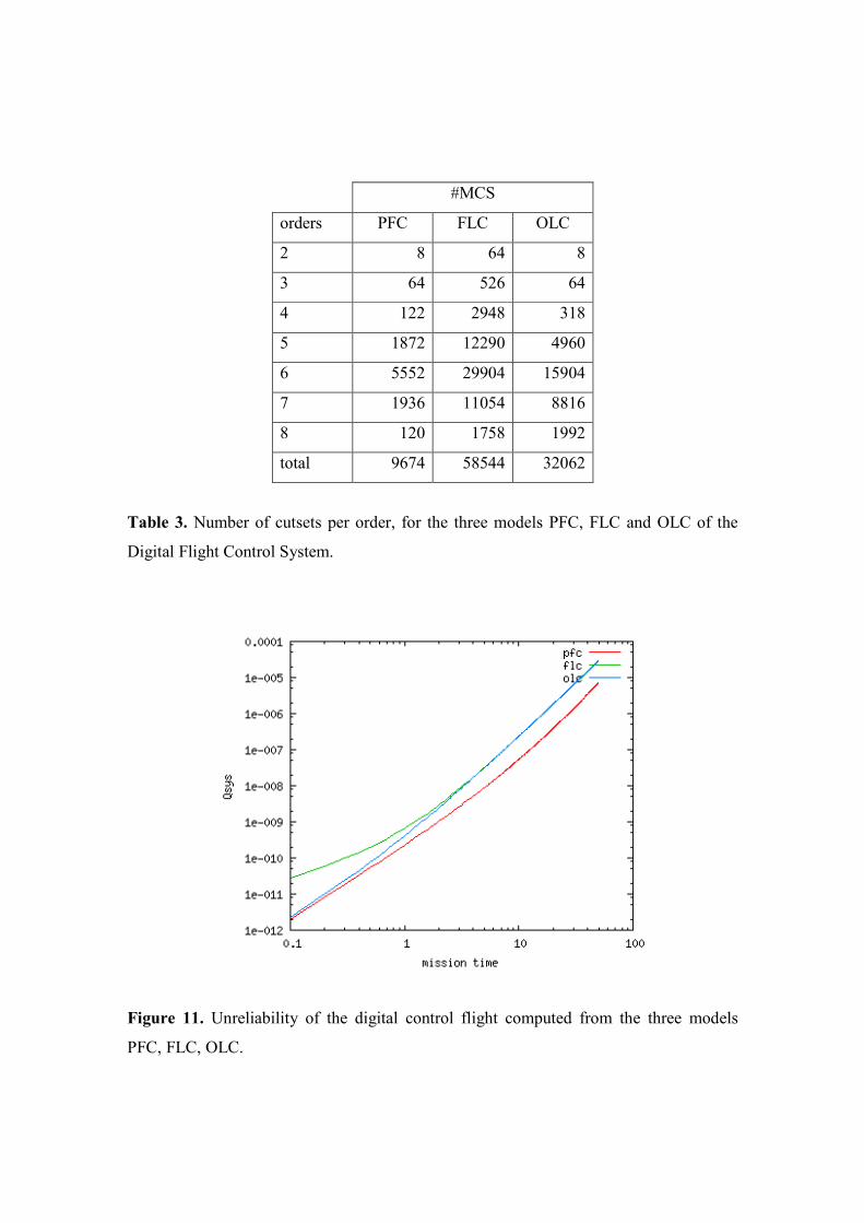
of failure. The estimated coverage levels for the various voted elements are summarized
in Table 1. The expected failure rates for each of the redundant element types are given in
Table 2 .
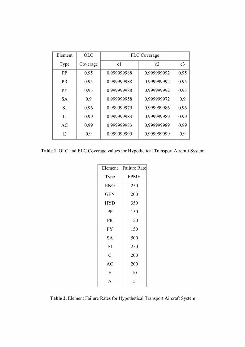
Figure 9 shows a functional block diagram for this hypothetical 4 engines transport
aircraft with a quadruple channel digital flight control system. This system has four
engines (ENGn), which provide power to the electrical generator/transformer rectifiers
(GENn) and hydraulic pumps (HYDn). Each of the GENn provide power to two
electrical buses (BUSn) which distribute direct current electrical power to each of the

electrically powered elements associated with its local channel. The flight control
computers (Cn) receive vehicle state information from two different sensor systems
associated with each channel, the air data system (SAn) and a strap-down inertial system
(SIn). Each axis of the pilot’s control wheel and rudder pedals has a quadruple set of
transducers, which provide pilot command data to the flight control computers. The pitch,
roll and yaw command transducers are designated, PPn, PRn and PYn respectively. The
Cn are interconnected via a cross-channel data link (CCDL), which allows the flight
control computers to send their local sensor data to each of the other computers, this
allows each of the Cn to "vote" sensor inputs. Each Cn then transmits a set of control
surface commands to its local actuation system computer, ACn. The ACn also have a
CCDL, allowing them to vote the inputs and their control surface commands. Each of the
ACn transmit the individual control surface commands to the actuation system
controlling each of the 8 flight control surfaces on the vehicle, these commands are
depicted in the figure as CHn.
Figure 10, provides a functional diagram for 1 of the 8 flight critical control surfaces
utilized by the vehicle. System operation requires all 8 of the control surfaces to be
operational. Each control surface utilizes two actuators, An. For the surface to be
operational at least 1-out-of-2 An must be operational. Each of the An can be supplied
hydraulic power from either of 2 hydraulic systems, Hn.
We designed a fault tree for this digital flight control system. The fault tree is made of 95
gates among which 15 are k-out-of-n:F IFC gates. We designed three versions of this
fault tree: one where the 15 gates are just k-out-of-n:F (PFC model), one with 15 FLC
gates and one with 15 OLC gates. The first tree involves 120 basic events, the second
one 186 basic events and the third one 143 basic events. The BDD for these three fault
trees are made respectively of 6796, 22778 and 12240 nodes. The number of minimal
cutsets (and their orders) of these three fault trees are given Table 3.
We computed the top event probability for mission times 0, 0.1, 0.2…, and 50 (total 501
points). The three curves are given Figure 11. This figure shows significant differences
between the PFC and the IFC models. It shows also that the OLC provides a very good
approximation of the full FLC model for mission times greater than 4. Note that there is
no significant difference between the unreliabilities computed from BDD and from MCS.
Running times to compute the BDD, the minimal cutsets and the unreliability curves
(from both BDD and MCS) are respectively 1.40 seconds, 4.42 seconds and 2.64 seconds
(on a desktop computer cadenced at 3.40GHz and running Windows XP). These running
times are quite good and show the efficiency of the approach we propose on a realistic
size test case.
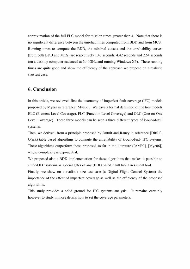
6. Conclusion
In this article, we reviewed first the taxonomy of imperfect fault coverage (IFC) models
proposed by Myers in reference [Mye06]. We gave a formal definition of the tree models
ELC (Element Level Coverage), FLC (Function Level Coverage) and OLC (One-on-One
Level Coverage). These three models can be seen a three different types of k-out-of-n:F
systems.
Then, we derived, from a principle proposed by Dutuit and Rauzy in reference [DR01],
O(n.k) table based algorithms to compute the unreliability of k-out-of-n:F IFC systems.
These algorithms outperform those proposed so far in the literature ([AM99], [Mye06])
whose complexity is exponential.
We proposed also a BDD implementation for these algorithms that makes it possible to
embed IFC systems as special gates of any (BDD based) fault tree assessment tool.
Finally, we show on a realistic size test case (a Digital Flight Control System) the
importance of the effect of imperfect coverage as well as the efficiency of the proposed
algorithms.
This study provides a solid ground for IFC systems analysis. It remains certainly
however to study in more details how to set the coverage parameters.
7. References
[AM99] S. V. Amari, J. B. Misra, A Seperable Method for Incorporating Imperfect Fault-
Coverage into Combinatorial Models, IEEE Transactions on Reliability, 48(3),
pages 267-274, September 1999.
[ADM99] S. V. Amari, J. B. Dugan, R. B. Misra, Optimal Reliability of Systems Subject
to Imperfect Fault-Coverage, IEEE Transactions on Reliability, 48(3), pages 275-
284, September 1999.
[BRB90] K. Brace, R. Rudell, and R. Bryant. Efficient Implementation of a BDD
Package. In Proceedings of the 27th ACM/IEEE Design Automation Conference,
pages 40–45. IEEE 0738, 1990.
[Bry86] R. Bryant. Graph Based Algorithms for Boolean Function Manipulation. IEEE
Transactions on Computers, 35(8):677–691, August 1986.
[Bry92] R. Bryant. Symbolic Boolean Manipulation with Ordered Binary Decision
Diagrams. ACM Computing Surveys, 24:293–318, September 1992.
[CAK02] Y-R Chang, S. V. Amari, S-Y Kuo, Reliability Evaluation of Multi-state
Systems Subject to Imperfect Coverage using OBDD, Proceedings of the 2002
Pacific Rim International Symposium on Dependable Computing IEEE.
[Dug89] J. B. Dugan, Fault Tree and Imperfect Coverage, IEEE Transactions on
Reliability, vol. 38, pages 177-185, March 1989.
[DDP95] S. A. Doyle, J. B. Dugan, F. A. Patterson-Hine, A Combinatorial Approach to
Modeling Imperfect Coverage, IEEE Transactions on Reliability, vol. 44, pages 87-
94, March 1995.
[DR00] Y. Dutuit and A. Rauzy. Efficient Algorithms to Assess Components and Gates
Importances in Fault Tree Analysis. Reliability Engineering and System Safety,
72(2):213–222, 2000.
[DR01] Y. Dutuit and A. Rauzy. New insights in the assessment of k-out-of-n and related
systems. Reliability Engineering and System Safety, 72(3):303–314, 2001.
[DT89] J. B. Dugan, K. S. Trivedi, Coverage Modeling for Dependability Analysis of
Fault-Tolerant Systems, IEEE Transactions on Reliability, vol. 38, pages 775-787,
June 1989.
[Mye06] A. F. Myers, k-out-of-n:G System Reliability with Imperfect Fault Coverage. To
Appear in IEEE Transactions On Reliability, 2006.
[Rau93] A. Rauzy. New Algorithms for Fault Trees Analysis. Reliability Engineering &
System Safety, 05(59):203–211, 1993.
[Rau01] A. Rauzy. Mathematical Foundation of Minimal Cutsets. IEEE Transactions on
Reliability, volume 50, number 4, pages 389-396, 2001.
[Tri02] K. S. Trivedi, Probability and Statistics with Reliability, Queuing and Computer
Science Applications, 2 ed, John Wiley & Sons, New York, 2002.
ELC(k,n)
// initialisation
for j = 1 upto k-1 do P[j] ← 0.0 done
P[0] ← 1.0, ELC ← 0.0
// main loop
for i = 1 upto n do
ELC ← ELC + pi*(1-ci) + pi*ci*P[k-1]
for j = k-1 downto 1 do
P[j] ← (1–pi)*P[j] + pi*ci*P[j-1]
done
P[0] ← (1–pi)*P[0]
done
return ELC
Figure 1. A table base algorithm to compute ELC(k,n)
FLC(n,k)
// initialisation
for j = 1 upto k-1 do P[j] ← 0.0 done
P[0] ← 1.0, FLC ← 0.0
// main loop
for i = 1 upto n do
FLC ← FLC + pi*P[k-1]
for j = k-1 downto 1 do
FLC ← FLC + pi*(1-cj)*P[j-1]
P[j] ← (1–pi)*P[j] + pi*cj*P[j-1]
done
P[0] ← (1–pi)*P[0]
done
return FLC
Figure 2. A table based algorithm to compute FLC(n,k)
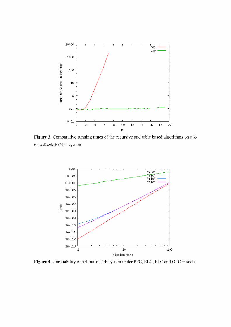
Figure 3. Comparative running times of the recursive and table based algorithms on a k-
out-of-4xk:F OLC system.
Figure 4. Unreliability of a 4-out-of-4:F system under PFC, ELC, FLC and OLC models
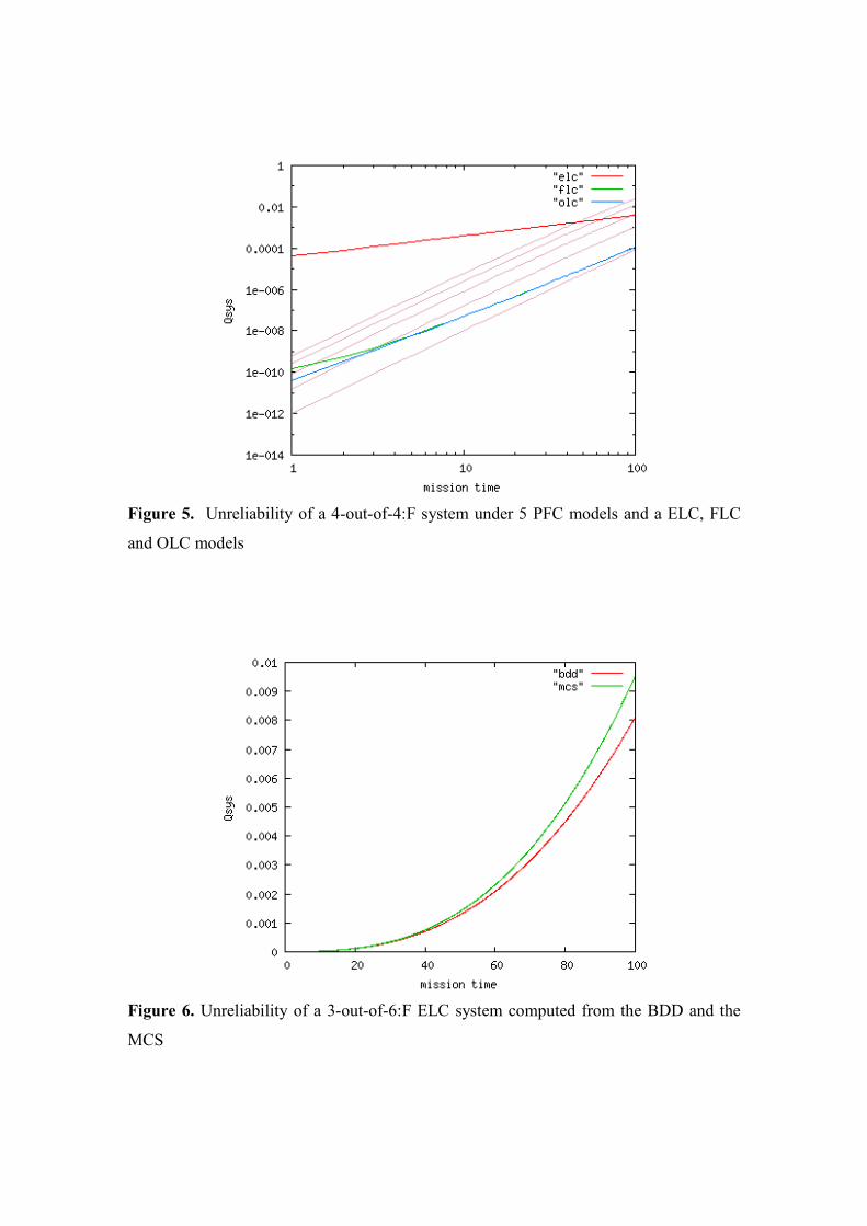
Figure 5. Unreliability of a 4-out-of-4:F system under 5 PFC models and a ELC, FLC
and OLC models
Figure 6. Unreliability of a 3-out-of-6:F ELC system computed from the BDD and the
MCS
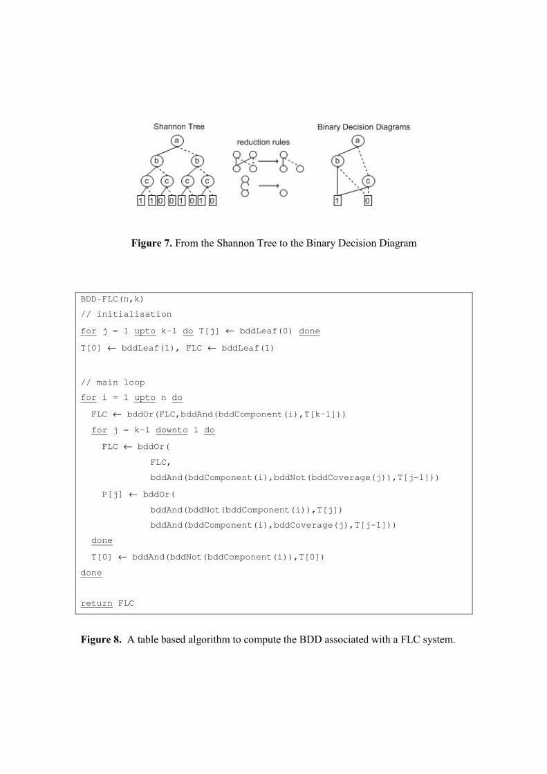
Figure 7. From the Shannon Tree to the Binary Decision Diagram
BDD-FLC(n,k)
// initialisation
for j = 1 upto k-1 do T[j] ← bddLeaf(0) done
T[0] ← bddLeaf(1), FLC ← bddLeaf(1)
// main loop
for i = 1 upto n do
FLC ← bddOr(FLC,bddAnd(bddComponent(i),T[k-1]))
for j = k-1 downto 1 do
FLC ← bddOr(
FLC,
bddAnd(bddComponent(i),bddNot(bddCoverage(j)),T[j-1]))
P[j] ← bddOr(
bddAnd(bddNot(bddComponent(i)),T[j])
bddAnd(bddComponent(i),bddCoverage(j),T[j-1]))
done
T[0] ← bddAnd(bddNot(bddComponent(i)),T[0])
done
return FLC
Figure 8. A table based algorithm to compute the BDD associated with a FLC system.
Element OLC FLC Coverage
Type Coverage c1 c2 c3
PP 0.95 0.999999988 0.999999992 0.95
PR 0.95 0.999999988 0.999999992 0.95
PY 0.95 0.999999988 0.999999992 0.95
SA 0.9 0.999999958 0.999999972 0.9
SI 0.96 0.999999979 0.999999986 0.96
C 0.99 0.999999983 0.999999989 0.99
AC 0.99 0.999999983 0.999999989 0.99
E 0.9 0.999999999 0.999999999 0.9
Table 1. OLC and ELC Coverage values for Hypothetical Transport Aircraft System
Element Failure Rate
Type FPMH
ENG 250
GEN 200
HYD 350
PP 150
PR 150
PY 150
SA 500
SI 250
C 200
AC 200
E 10
A 5
Table 2. Element Failure Rates for Hypothetical Transport Aircraft System
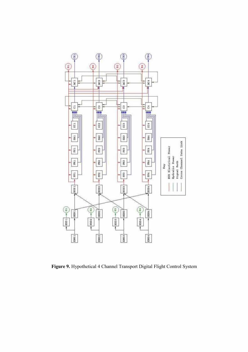
Figure 9. Hypothetical 4 Channel Transport Digital Flight Control System
Figure 10. Actuation System for a Hypothetical Transport Aircraft Control Surface
#MCS
orders PFC FLC OLC
2 8 64 8
3 64 526 64
4 122 2948 318
5 1872 12290 4960
6 5552 29904 15904
7 1936 11054 8816
8 120 1758 1992
total 9674 58544 32062
Table 3. Number of cutsets per order, for the three models PFC, FLC and OLC of the
Digital Flight Control System.
Figure 11. Unreliability of the digital control flight computed from the three models
PFC, FLC, OLC.