The views expressed herein are those of the authors and do not necessarily reflect the views of CBBEP or other organizations that may have provided funding for this project.

 

 

 

 

 

 

 

Assessment of Seagrass Habitat Quality and Plant Physiological Conditions in South Texas Waters

Publication CBBEP – 80 Project Number – 1201

July 2012

Prepared by Christopher J. Wilson and Kenneth H. Dunton

The University of Texas at Austin Marine Science Institute, 750 Channel View Drive, Port Aransas, TX 78373 Phone: (361) 749-6744

Email: ken.dunton@mail.utexas.edu

Submitted to:

Coastal Bend Bays & Estuaries Program 1305 N. Shoreline Blvd. Ste 205

Corpus Christi, Texas 78401

1

Assessment of seagrass habitat quality and plant physiological condition in Texas coastal waters

Christopher J. Wilson and Kenneth H. Dunton1

1The University of Texas at Austin Marine Science Institute, 750 Channel View Drive, Port Aransas, TX 78373 Email: ken.dunton@mail.utexas.edu Phone: (361) 749-6744

2

TABLE OF CONTENTS

Project Summary 3 Introduction 4 Methods 6 Sampling Summary 6 Site Selection 6 Water Quality 7 Seagrass Coverage 7 Plant Tissue Condition 7 Spatial Data Analysis and Interpolation 8 Results 9 Water Quality 9 Water Transparency 14

Seagrass Coverage and Species Distributions 18 Plant Tissue Condition 24 Conclusions 33 Water Quality 33 Water Transparency 34

Seagrass Coverage and Species Distributions 34 Plant Tissue Condition 35 Future Recommendations 37 References 39 Appendix 40

3

PROJECT SUMMARY

This report details the results of the Texas Seagrass Monitoring Plan following the survey of 567 individual sampling stations during the summer and early fall of 2011. Sampling station locations were chosen from seagrass meadows mapped from remotely sensed data obtained from the 2004/2007 NOAA Benthic Habitat Assessment. Stations were spatially distributed among three estuarine systems: the Mission-Aransas, Nueces, and Laguna Madre. These three estuarine systems contain about 94% of the seagrasses along the Texas coast. The 2011 field sampling effort specifically implemented Tier 2 protocols, which are intended to provide rapid assessments of hydrography, seagrass areal coverage, species distributions and plant physiological conditions. The observational data obtained during the field survey was then illustrated using geographic information systems in order to evaluate spatial relationships in measured parameters. The Tier 2 sampling program successfully yielded spatial characteristics of seagrass habitat quality, identified regions exhibiting seagrass decline and thoroughly evaluated the validity of seagrass habitat described in the 2004/2007 NOAA Benthic Habitat Assessment.

4

INTRODUCTION

In 1999, the Texas Parks and Wildlife Department (TPWD), along with the Texas General Land Office (TGLO) and the Texas Commission on Environmental Quality (TCEQ), drafted a Seagrass Conservation Plan. Part of this plan proposed a seagrass habitat monitoring program (Pulich and Calnan, 1999), with one of the main recommendations being to develop a coast-wide monitoring program. In response, the Texas Seagrass Monitoring Plan (TSGMP) proposed a monitoring effort to detect changes in seagrass ecosystem conditions prior to actual seagrass mortality (Pulich et al., 2003). However, implementation of the plan required additional research to specifically identify the environmental parameters that elicit a seagrass stress response and the physiological or morphological variables that best reflect the impact of these environmental stressors.

Numerous researchers have related seagrass health to environmental stressors; however, these studies have not arrived at a consensus regarding the most effective habitat quality and seagrass condition indicators. Kirkman (1996) recommended biomass, productivity, and density for monitoring seagrass whereas other researchers focused on changes in seagrass distribution as a function of environmental stressors (Dennison et al., 1993, Livingston et al., 1998, Koch 2001, and Fourqurean et al., 2003). The consensus among these studies revealed that salinity, depth, light, nutrient concentrations, sediment characteristics, and temperature were among the most important variables that produced a response in a measured seagrass indicator. The relative influence of these environmental variables is likely a function of the seagrass species in question, the geographic location of the study, hydrography, methodology, and other factors specific to local climatology. Because no generalized approach can be extracted from previous research, careful analysis of regional seagrass ecosystems is necessary to develop an effective monitoring program for Texas.

Conservation efforts should seek to develop a conceptual model that outlines the linkages among seagrass ecosystem components and the role of indicators as predictive tools to assess the seagrass physiological response to stressors at various temporal and spatial scales. Tasks for this objective include the identification of stressors that arise from human-induced disturbances, which can result in seagrass loss or compromise plant physiological condition. For example, stressors that lead to higher water turbidity and light attenuation (e.g. dredging and shoreline erosion) are known to result in lower below-ground seagrass biomass and alterations to sediment nutrient concentrations. It is therefore necessary to evaluate long-term light measurements, the biomass of above- versus below-ground tissues, and the concentrations of nutrients, sulfides and dissolved

5

oxygen in sediment porewaters when examining the linkages between light attenuation and seagrass health.

This study implements a program for monitoring seagrass meadows in Texas coastal waters following protocols that evaluate seagrass conditions based on landscape-scale dynamics. These protocols adhere to the hierarchical strategy for seagrass monitoring outlined by Neckles et al. (2012) and serve to establish quantitative relationships between physical and biotic parameters that ultimately control seagrass condition, distribution, persistence, and overall health. Our monitoring approach follows a broad template adopted by several federal and state agencies across the country, but which is uniquely designed for Texas (Dunton et al., 2011) and integrates plant condition indicators with landscape feature indicators to detect and interpret seagrass bed disturbances.

The objectives of this study were to (1) implement long-term monitoring to detect environmental changes with a focus on the ecological integrity of seagrass habitats, (2) provide insight to the ecological consequences of these changes, and (3) help decision makers (e.g. various state and federal agencies) determine if the observed change necessitates a revision of regulatory policy or management practices. We defined ecological integrity as the capacity of the seagrass system to support and maintain a balanced, integrated, and adaptive community of flora and fauna including its historically characteristic seagrass species. Ecological integrity was assessed using a suite of condition indicators (physical, biological, hydrological, and chemical) measured on different spatial and temporal scales.

The primary questions addressed in the 2011 annual Tier 2 survey include: 1) What are the spatial and temporal patterns in the distribution of seagrasses

over annual and decadal scales? 2) What are the characteristics of these plant communities, including their

species composition and percent cover? 3) How are any changes in seagrass percent cover and species composition

related to measured characteristics of water quality?

6

METHODS

Sampling Summary

Tier 2 protocols, which are considered Rapid Assessment sampling methods, are adapted from Neckles et al. (2012). Tier 2 sampling began in late summer 2011 and was completed by early October 2011. For statistical rigor, a repeated measures design with fixed sampling stations was implemented to maximize our ability to detect future change. Neckles et al. (2012) demonstrated that the Tier 2 approach, when all sampling stations are considered together within a regional system, results in >99% probability that the bias in overall estimates will not interfere with detection of change. Site Selection

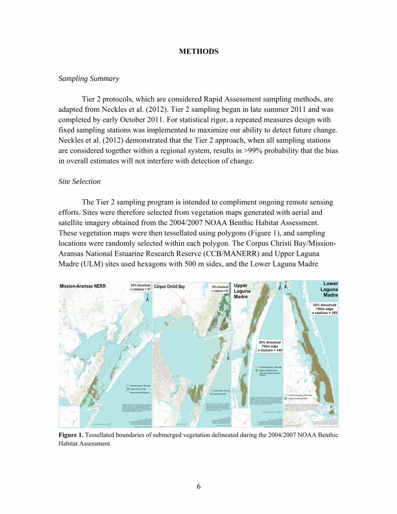
The Tier 2 sampling program is intended to compliment ongoing remote sensing efforts. Sites were therefore selected from vegetation maps generated with aerial and satellite imagery obtained from the 2004/2007 NOAA Benthic Habitat Assessment. These vegetation maps were then tessellated using polygons (Figure 1), and sampling locations were randomly selected within each polygon. The Corpus Christi Bay/Mission-Aransas National Estuarine Research Reserve (CCB/MANERR) and Upper Laguna Madre (ULM) sites used hexagons with 500 m sides, and the Lower Laguna Madre

Figure 1. Tessellated boundaries of submerged vegetation delineated during the 2004/2007 NOAA Benthic Habitat Assessment.

7

(LLM) site used hexagons with 750 m sides. Only polygons containing over 50% seagrass coverage were included in the 2011 sampling effort. Water Quality

All sampling stations were located in the field using a hand-held GPS device to within a 10 m radius of the pre-determined station coordinates. Upon arrival to a station, hydrographic measurements including water depth, conductivity, temperature, salinity, dissolved oxygen, chlorophyll fluorescence and pH were collected with a YSI 600XL data sonde. Replicate water samples were obtained at each station for determination of Total Suspended Solid (TSS) concentration (See Appendix A.1). Water transparency was derived from measurements of photosynthetically active radiation (PAR) using two LI-COR spherical quantum scalar sensors attached to a lowering frame (See Appendix A.2). All sonde measurements and water samples were obtained prior to the deployment of benthic sampling equipment. Seagrass Coverage

Species composition and areal coverage were obtained from four replicate quadrat samples per station at each of the four cardinal locations from the vessel. Percent cover of areal biomass was estimated by direct observation, looking down at the seagrass canopy through the water using a 0.25 m2

quadrat framer subdivided into 100 cells. Previous research has demonstrated that the probability of a bias in the overall mean when using four subsamples is <5% (Neckles, pers. comm.). Plant Tissue Condition

Seagrass leaf tissue was collected at every station containing a vegetated bottom. Upon removal, all tissue samples were immediately placed on ice in sealed plastic containers and transported to the University of Texas at Austin Marine Science Institute (UTMSI). Leaf tissue samples were then dried to a constant weight in a 60°C oven and homogenized using a mortar and pestle. Leaf tissue phosphorous content was determined at UTMSI (See Appendix A.3), and subsamples of leaf tissue were sent to the University of California at Davis for determination of leaf tissue carbon content, nitrogen content, δ13C and δ15N (See Appendix A.3). Tissue constituent ratios are represented on a molar basis. All plant tissue analysis was limited to Halodule wrightii, as this species was the most prevalent and widely distributed among sample sites. A single species was chosen to reduce confounding factors attributed to plant physiology and to provide a reliable metric amenable to spatial comparisons.

8

Spatial Data Analysis and Interpolation

ArcGIS software was used to manage, analyze, and display spatially referenced point samples and interpolate surfaces for all measured parameters. An inverse distance- weighted method was used to assign a value to areas (cells) between sampling points. A total of 12 sampling stations were identified from a variable search radius to generate the value for a single unknown output cell (100 m2). All data interpolation was spatially restricted to the geographic limits of the submerged vegetation map created during the 2004/2007 NOAA Benthic Habitat Assessment.

9

RESULTS

Water Quality

Corpus Christi Bay/Mission-Aransas National Estuarine Research Reserve The CCB/MANERR site exhibited a depth of 51.2 ± 23.2 cm (mean ± standard

deviation; Table 1, Figure 2a), and was the most shallow of the three regions surveyed in 2011. This site also exhibited the smallest spatial variation in depth. Salinity varied the least among sampling stations at this site, with a mean of 41.80 ± 3.90 ppt (Table 1, Figure 2b). Very low salinity values (<10 ppt) were observed along the southern border of Copano Bay, while several regions of hypersaline water were documented along the northeastern border of Redfish Bay and the easternmost boundary of CCB. This region had the second highest dissolved oxygen concentration, with a mean of 6.39 ± 2.00 mg L-1 (Table 1, Figure 2c). The lowest dissolved oxygen concentrations were documented in the northeastern boundary of CCB, within East Flats. One sampling station had a dissolved oxygen concentration indicative of hypoxic conditions (<2 mg L-1), while four additional stations revealed concentrations below 3 mg L-1. Lastly, the CCB/MANERR site had the lowest and most variable pH values (7.85 ± 0.38; Figure 2d) and the only acidic pH value (6.79) for any region. The pH was lowest in the Aransas and Copano Bays and gradually increased southwards into CCB.

Upper Laguna Madre

The ULM site had a mean depth of 81.7 ± 42.0 cm (Table 1, Figure 2a) and

varied the most spatially among the three sites surveyed. The ULM exhibited the highest salinity of all sites with a mean of 49.32 ± 6.90 ppt (Table 1; Figure 2b). It is interesting to note that the maximum salinity values were observed south of Baffin Bay on the eastern side of the land cut. This area is essentially in the center of the Laguna Madre and lies at the greatest distance from a significant tidal inlet or freshwater source. As a result, these high salinity values are likely attributed to long water residence times. The ULM had the lowest mean dissolved oxygen concentration of any site (5.33 ± 2.06 mg L-1; Table 1, Figure 2c). Hypoxic conditions were observed at five sampling stations, while an additional nine stations recorded dissolved oxygen concentrations less than 3 mg L-1. The highest dissolved oxygen concentrations were observed at the northern mouth of Baffin Bay, and the lowest concentrations were found to the south of Baffin Bay and the interior ULM between Baffin and Corpus Christi Bays. Finally, the ULM recorded a mean pH of (7.96 ± 0.34; Figure 2d), with the lowest values generally observed at Mustang Island State Park and to the west of the Intracoastal Waterway.

10

Lower Laguna Madre The LLM contained the deepest seagrass habitat of the three sites surveyed with a

mean depth of 84.1 ± 36.2 cm (Table 1, Figure 2a). This site was the least saline with a mean salinity of 41.64 ± 3.88 ppt (Table 1, Figure 2b). The lowest salinities were observed in areas to the north of the Port Mansfield and Brazos Santiagos Passes, while the highest salinities were observed in the El Realito Bay and in the interior section of the LLM, furthest from navigational passes. The LLM site contained the highest mean dissolved oxygen concentration of any site (7.17 ± 1.28 mg L-1; Table 1, Figure 2c). There were no documented instances of hypoxia and only one sampling station recorded a dissolved oxygen concentration less than 3 mg L-1. Dissolved oxygen concentrations were highest to the south of the Port Mansfield Pass and lowest to the east of Laguna Atascosa Wildlife Refuge and within Lake Verdolaga. Lastly, the LLM exhibited the highest and least variable pH of all three sites (8.09 ± 0.25; Figure 2d), with a slight decrease in pH from north to south.

11

Table 1. Summary of water quality parameters by region.

Depth (cm)

Dissolved Oxygen (mg L-1)

Salinity (ppt)

pH

CCB/NERR Mean 51.2 6.39 41.80 7.85 Standard Deviation 23.2 2.00 3.90 0.38 n 138 137 138 138

ULM Mean 81.7 5.33 49.32 7.96 Standard Deviation 42.0 2.06 6.90 0.34 n 144 142 142 143

LLM Mean 84.1 7.17 41.64 8.09 Standard Deviation 36.2 1.28 3.88 0.25 n 285 282 284 285

12

2a. 2b.

13

2c. 2d.

Figure 2. Spatial representations of a) water depth, b) salinity, c) dissolved oxygen and d) pH from the 2011 sampling effort. The spatial data interpolation is limited to the boundaries of seagrass habitat delineated during the 2004/2007 NOAA Benthic Habitat Assessment.

14

Water Transparency

Corpus Christi Bay/Mission-Aransas National Estuarine Research Reserve The CCB/MANERR site was characterized by the highest water clarity of all sites

with a mean downward attenuation coefficient (Kd) of 0.70 ± 0.53 m-1 (Table 2, Figure 3). The highest attenuation values were generally recorded at the northeastern boundary of Aransas Bay and in the westernmost CCB near Portland. Light attenuation is likely attributed to chlorophyll in the water column, as this site had the highest average chlorophyll (4.62 ± 2.86 μg L-1; Table 2, Figure 4a) and lowest average TSS (13.72 ± 8.74 mg L-1; Table 2, Figure 4b) concentrations of any site. Based on the mean Kd value observed in 2011, seagrasses in this region become limited by light availability at a depth of 2.44 m (assuming a surface irradiance of 2000 μmol photons m-2 s-1 and a minimum light requirement of 18% of surface irradiance).

Upper Laguna Madre

The ULM exhibited a mean Kd of 0.73 ± 0.33 m-1 (Table 2, Figure 3), which was

the least variable among sites. Similarly, water column chlorophyll (3.92 ± 2.07 μg L-1; Table 2, Figure 4a) and TSS (13.75 ± 7.11 mg L-1; Table 2, Figure 4b) also exhibited the least amount of spatial variation. Interestingly, the highest Kd values are located to the southeast of Laguna Larga and correspond to an area of high chlorophyll concentrations. Based on the mean Kd value observed in 2011, seagrasses in this region become limited by light availability at a depth of 2.34 m (assuming a surface irradiance of 2000 μm photons m-2 s-1 and a minimum light requirement of 18% of surface irradiance).

Lower Laguna Madre

The LLM had the lowest and most variable water clarity of any site (Kd = 1.39 ±

0.97 m-1; Table 2, Figure 3). This site also recorded the lowest mean chlorophyll (2.70 ± 3.05 μg L-1; Table 2, Figure 4a) and highest mean TSS (26.05 ± 33.36 mg L-1; Table 2, Figure 4b) concentrations of any site. The highest attenuation coefficients were observed at the southern entrance to the land cut, southwest of Port Mansfield and northeast of the Laguna Atascosa Wildlife Refuge. Each of these locations also exhibited very high concentrations of water column chlorophyll and TSS, which is undoubtedly responsible for the observed spatial patterns in light attenuation. Based on the mean Kd value observed in 2011, seagrasses in this region become limited by light availability at a depth of 1.24 m (assuming a surface irradiance of 2000 μm photons m-2 s-1 and a minimum light requirement of 18% of surface irradiance).

15

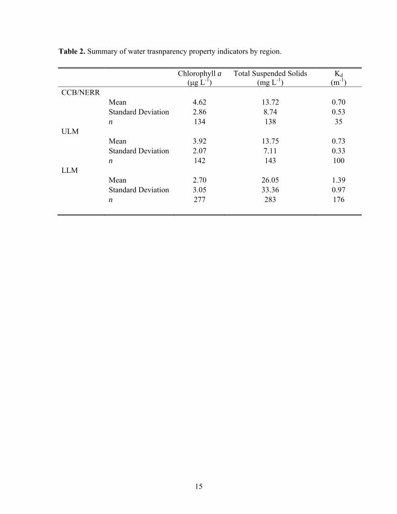
Table 2. Summary of water trasnparency property indicators by region.

Chlorophyll a

(μg L-1) Total Suspended Solids

(mg L-1) Kd

(m-1) CCB/NERR

Mean 4.62 13.72 0.70 Standard Deviation 2.86 8.74 0.53 n 134 138 35

ULM Mean 3.92 13.75 0.73 Standard Deviation 2.07 7.11 0.33 n 142 143 100

LLM Mean 2.70 26.05 1.39 Standard Deviation 3.05 33.36 0.97 n 277 283 176

16

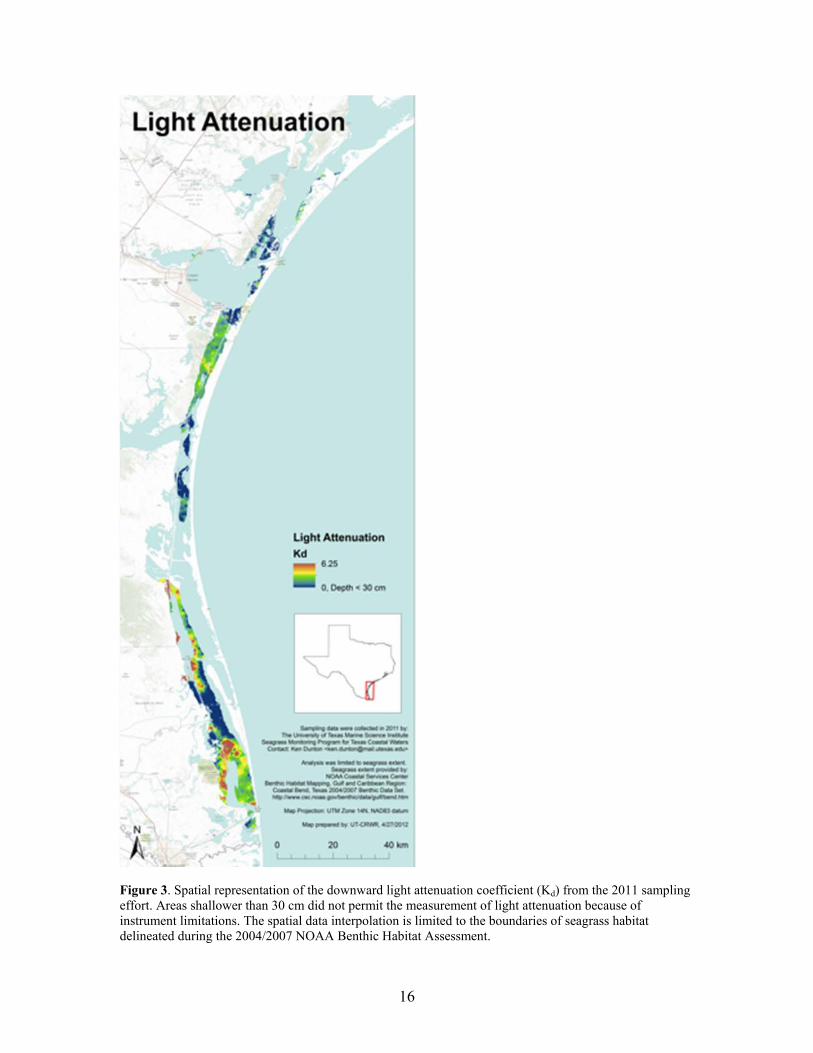
Figure 3. Spatial representation of the downward light attenuation coefficient (Kd) from the 2011 sampling effort. Areas shallower than 30 cm did not permit the measurement of light attenuation because of instrument limitations. The spatial data interpolation is limited to the boundaries of seagrass habitat delineated during the 2004/2007 NOAA Benthic Habitat Assessment.

17

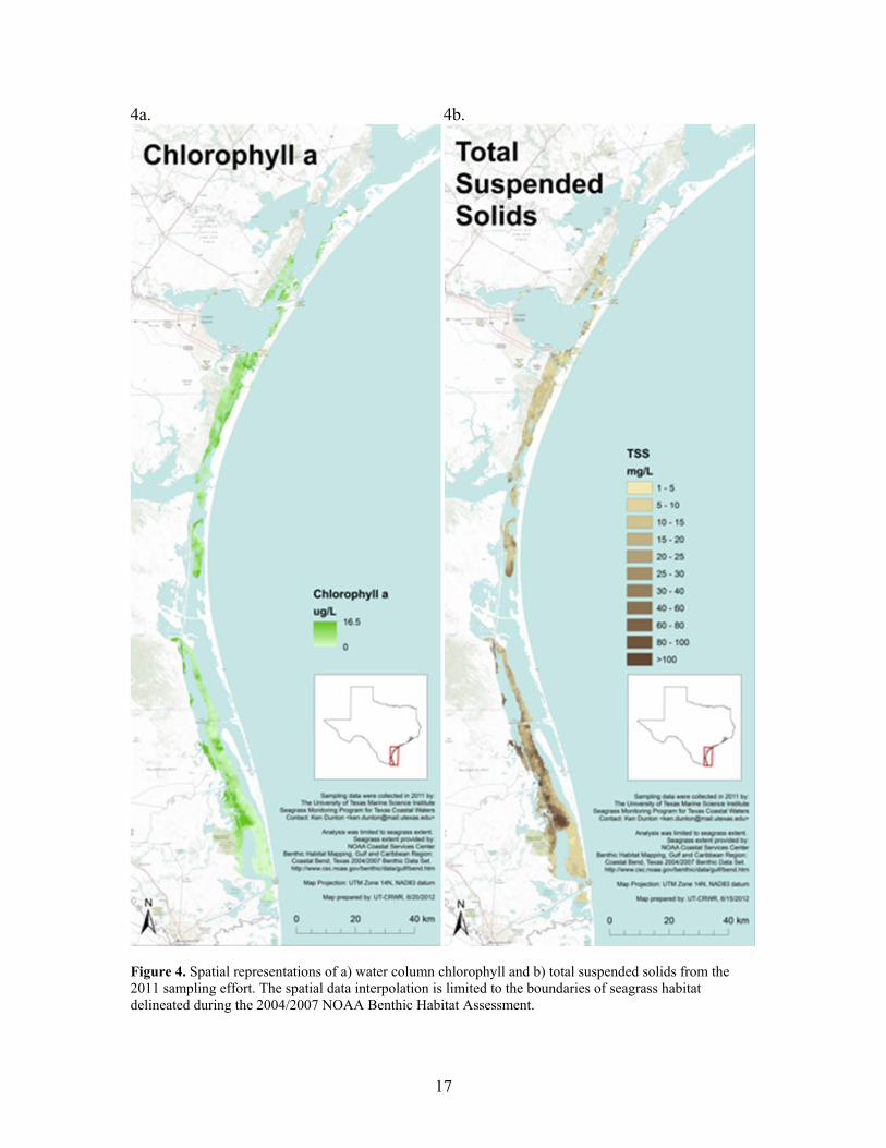
4a. 4b.

Figure 4. Spatial representations of a) water column chlorophyll and b) total suspended solids from the 2011 sampling effort. The spatial data interpolation is limited to the boundaries of seagrass habitat delineated during the 2004/2007 NOAA Benthic Habitat Assessment.

18

Seagrass Coverage and Species Distributions

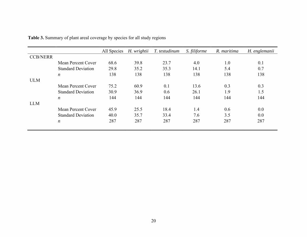
Corpus Christi Bay/Mission-Aransas National Estuarine Research Reserve Seagrasses covered a mean area of 68.6 ± 29.8% of the benthos in the

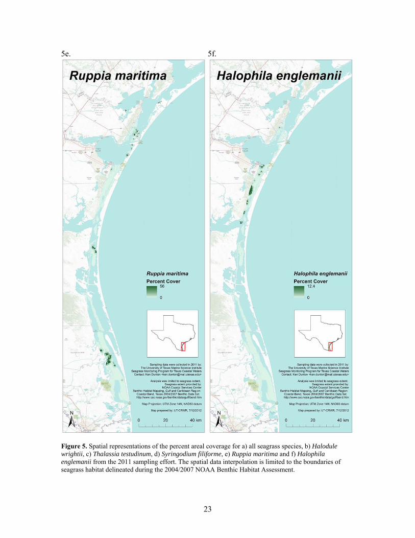
CCB/MANERR site (Table 3, Figure 5a). The seagrass assemblage was dominated by Halodule wrightii (39.8 ± 35.2%; Table 3, Figure 5b), followed by Thalassia testudinum (23.7 ± 35.3%; Table 3, Figure 5c), Syringodium filiforme (4.0 ± 14.1%; Table 3, Figure 5d), Ruppia maritima (1.0 ± 5.4%; Table 3, Figure 5e) and Halophila englemanii (0.1 ± 0.7%; Table 3, Figure 5f). Four sampling stations did not contain any vegetation and 5.8% of the stations in this site contained less than 10% seagrass coverage. Seagrass coverage was lowest along St. Joseph Island, near the Ingleside Naval Base and in the Nueces Bay near Portland. Halodule wrightii was distributed throughout the CCB/MANERR region, with the exception of Redfish Bay, where Thalassia testudinum dominated. Established Thalassia testudinum populations are likely excluding Halodule wrightii from expanding into this area.

Upper Laguna Madre

Seagrasses covered a mean area of 75.2 ± 30.9% of the benthos in the ULM site

(Table 3, Figure 5a). The seagrass assemblage was again dominated by Halodule wrightii (60.9 ± 36.9%; Table 3, Figure 5b), followed by Syringodium filiforme (13.6 ± 26.1%; Table 3, Figure 5c), Halophila englemanii (0.3 ± 1.5%; Table 3, Figure 5f), Ruppia maritima (0.3 ± 1.9%; Table 3, Figure 5e) and Thalassia testudinum (0.1 ± 0.6%; Table 3, Figure 5c). Seven sampling stations in this site did not contain any seagrass coverage, and 6.9% of the stations contained less than 10% seagrass coverage. Seagrass coverage was lowest to the southeast of the Nueces-Kleberg County line and south of Baffin Bay to the east of the land cut. Halodule wrightii was found throughout the ULM, but was lower in abundance to the east of Chapman Ranch. However, this area contained extensive cover of Syringodium filiforme. It does not initially appear that Syringodium filiforme is excluding Halodule wrightii because these two species were observed interspersed throughout the ULM. Lastly, the ULM site contained the greatest coverage of Halophila englemanii, with a distinguished population located to the east of Laguna Larga.

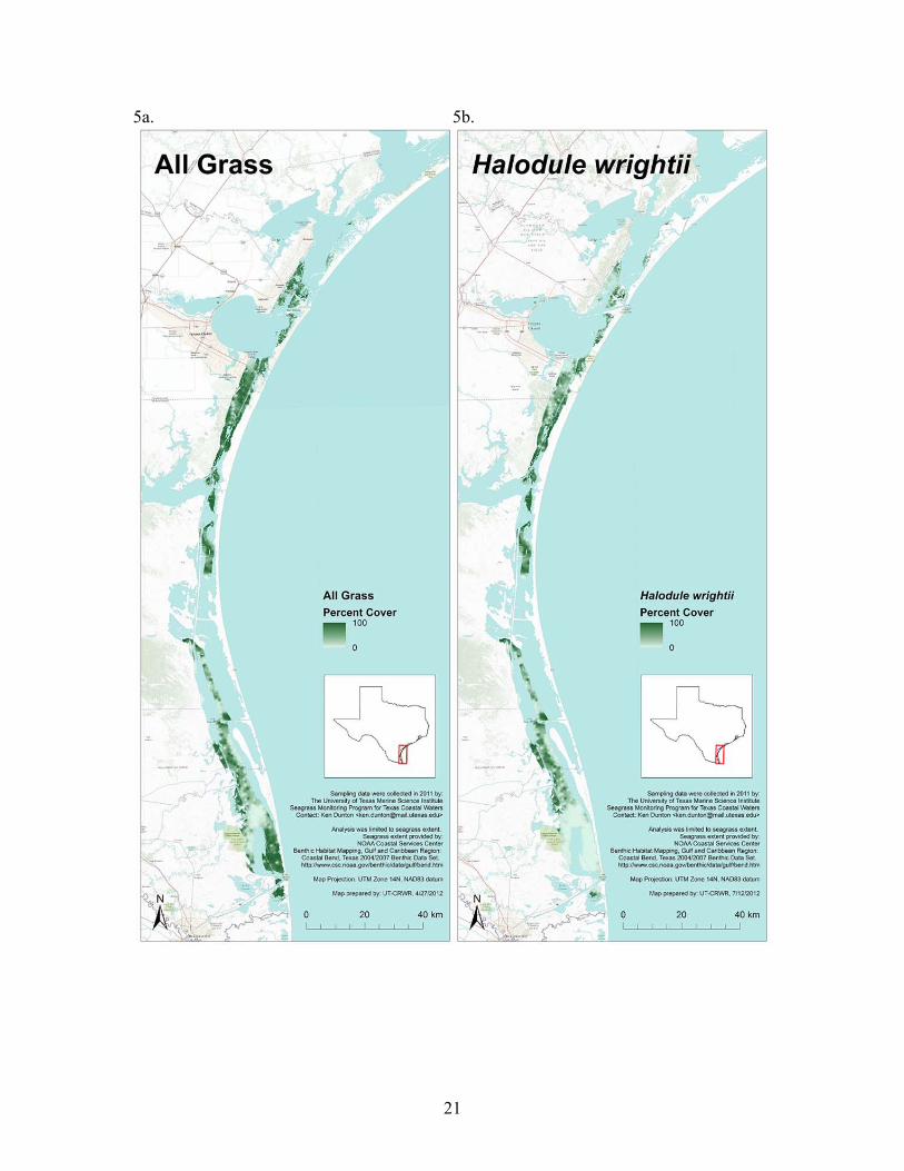
Lower Laguna Madre

Seagrasses covered a mean area of 45.9 ± 40.0% of the benthos in the LLM

region (Table 3, Figure 5a). The seagrass assemblage was dominated by Halodule wrightii (25.5 ± 35.7%; Table 3, Figure 5b), followed by Thalassia testudinum (18.4 ±

19

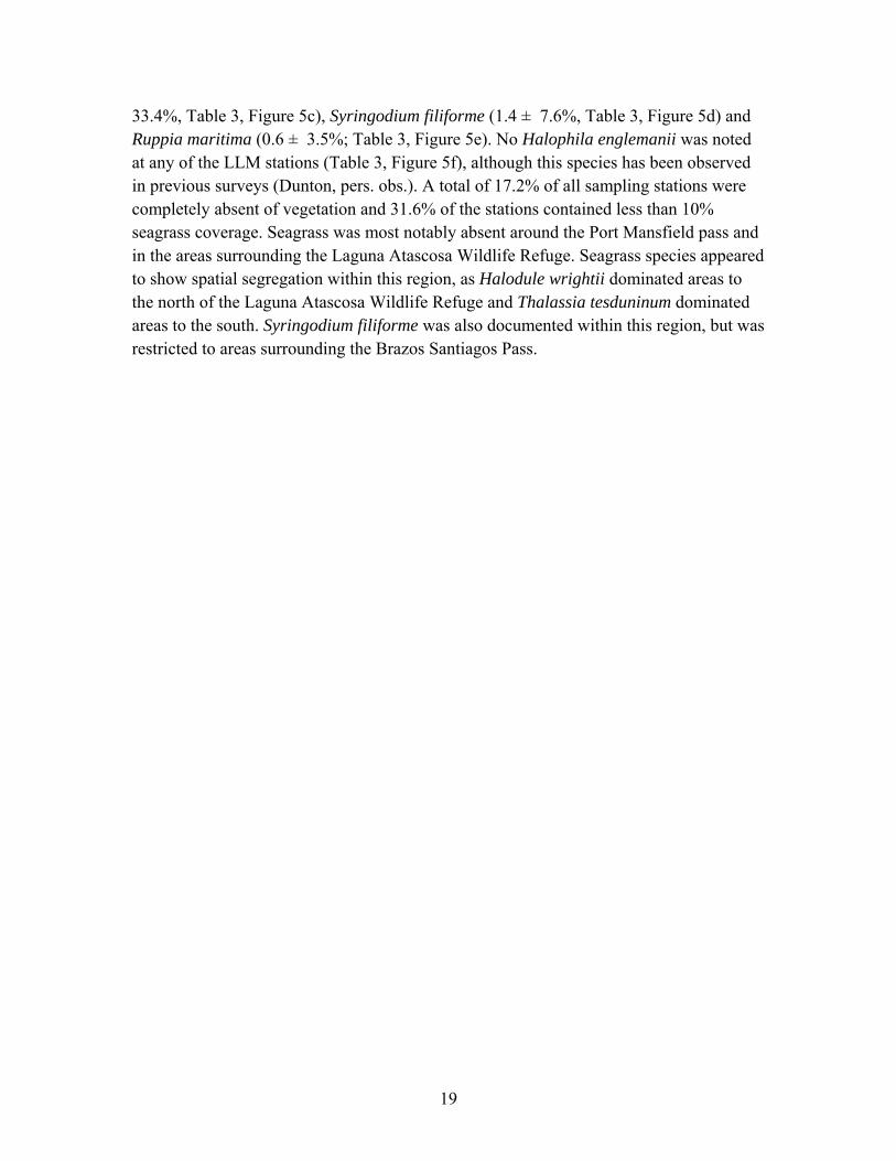
33.4%, Table 3, Figure 5c), Syringodium filiforme (1.4 ± 7.6%, Table 3, Figure 5d) and Ruppia maritima (0.6 ± 3.5%; Table 3, Figure 5e). No Halophila englemanii was noted at any of the LLM stations (Table 3, Figure 5f), although this species has been observed in previous surveys (Dunton, pers. obs.). A total of 17.2% of all sampling stations were completely absent of vegetation and 31.6% of the stations contained less than 10% seagrass coverage. Seagrass was most notably absent around the Port Mansfield pass and in the areas surrounding the Laguna Atascosa Wildlife Refuge. Seagrass species appeared to show spatial segregation within this region, as Halodule wrightii dominated areas to the north of the Laguna Atascosa Wildlife Refuge and Thalassia tesduninum dominated areas to the south. Syringodium filiforme was also documented within this region, but was restricted to areas surrounding the Brazos Santiagos Pass.

20

Table 3. Summary of plant areal coverage by species for all study regions

All Species H. wrightii T. testudinum S. filiforme R. maritima H. englemanii CCB/NERR

Mean Percent Cover 68.6 39.8 23.7 4.0 1.0 0.1 Standard Deviation 29.8 35.2 35.3 14.1 5.4 0.7 n 138 138 138 138 138 138

ULM Mean Percent Cover 75.2 60.9 0.1 13.6 0.3 0.3 Standard Deviation 30.9 36.9 0.6 26.1 1.9 1.5 n 144 144 144 144 144 144

LLM Mean Percent Cover 45.9 25.5 18.4 1.4 0.6 0.0 Standard Deviation 40.0 35.7 33.4 7.6 3.5 0.0 n 287 287 287 287 287 287

21

5a. 5b.

22

5c. 5d.

23

5e. 5f.

Figure 5. Spatial representations of the percent areal coverage for a) all seagrass species, b) Halodule wrightii, c) Thalassia testudinum, d) Syringodium filiforme, e) Ruppia maritima and f) Halophila englemanii from the 2011 sampling effort. The spatial data interpolation is limited to the boundaries of seagrass habitat delineated during the 2004/2007 NOAA Benthic Habitat Assessment.

24

Plant Tissue Condition

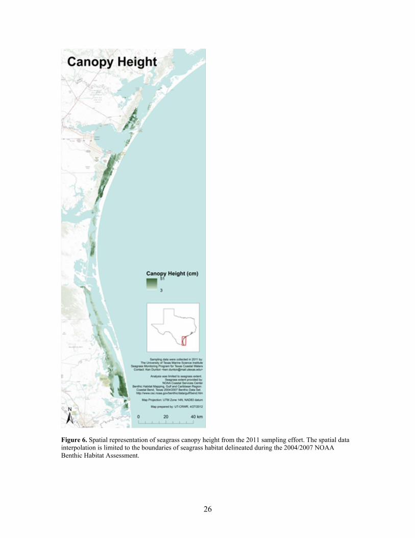
Corpus Christi Bay/Mission-Aransas National Estuarine Research Reserve The CCB/MANERR site contained the highest and most variable canopy height

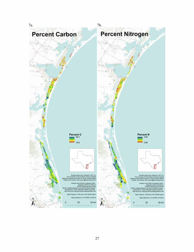
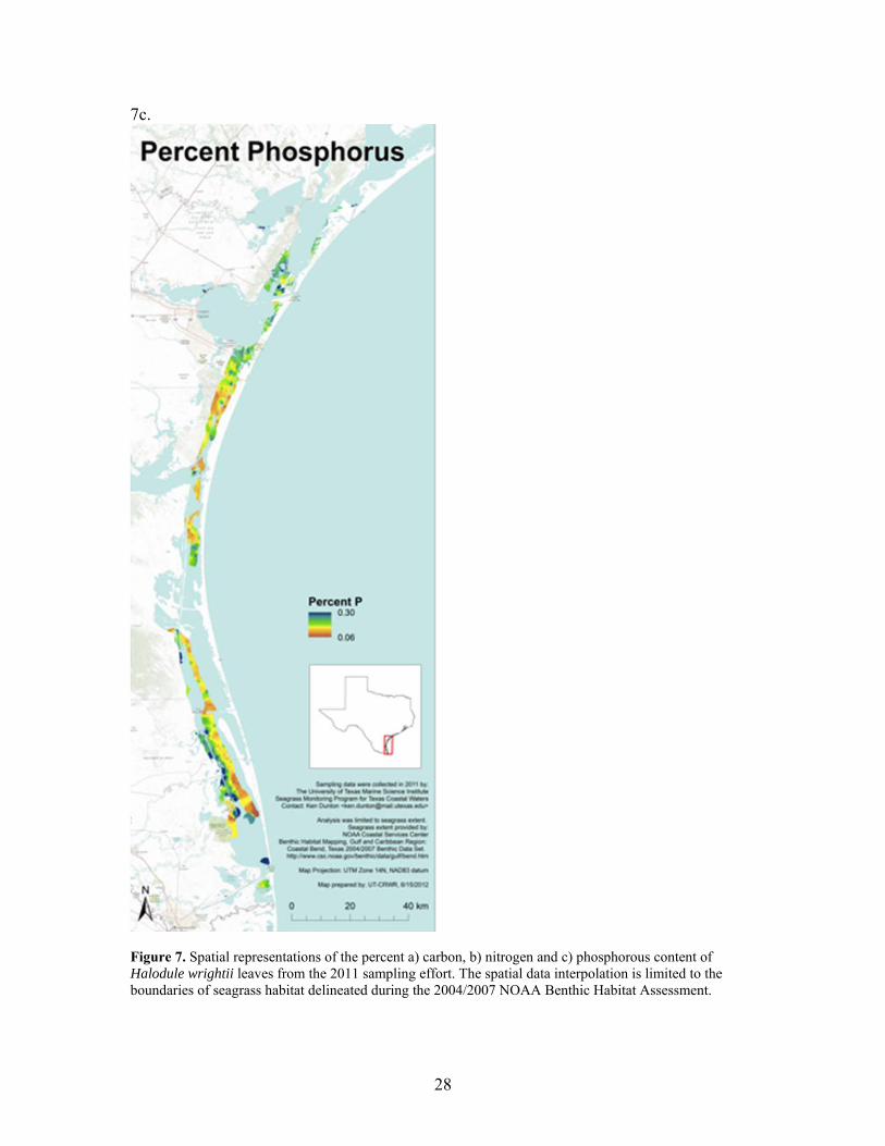
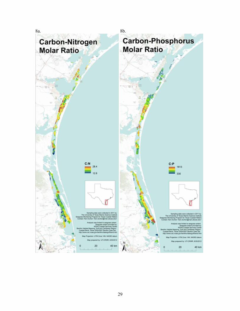
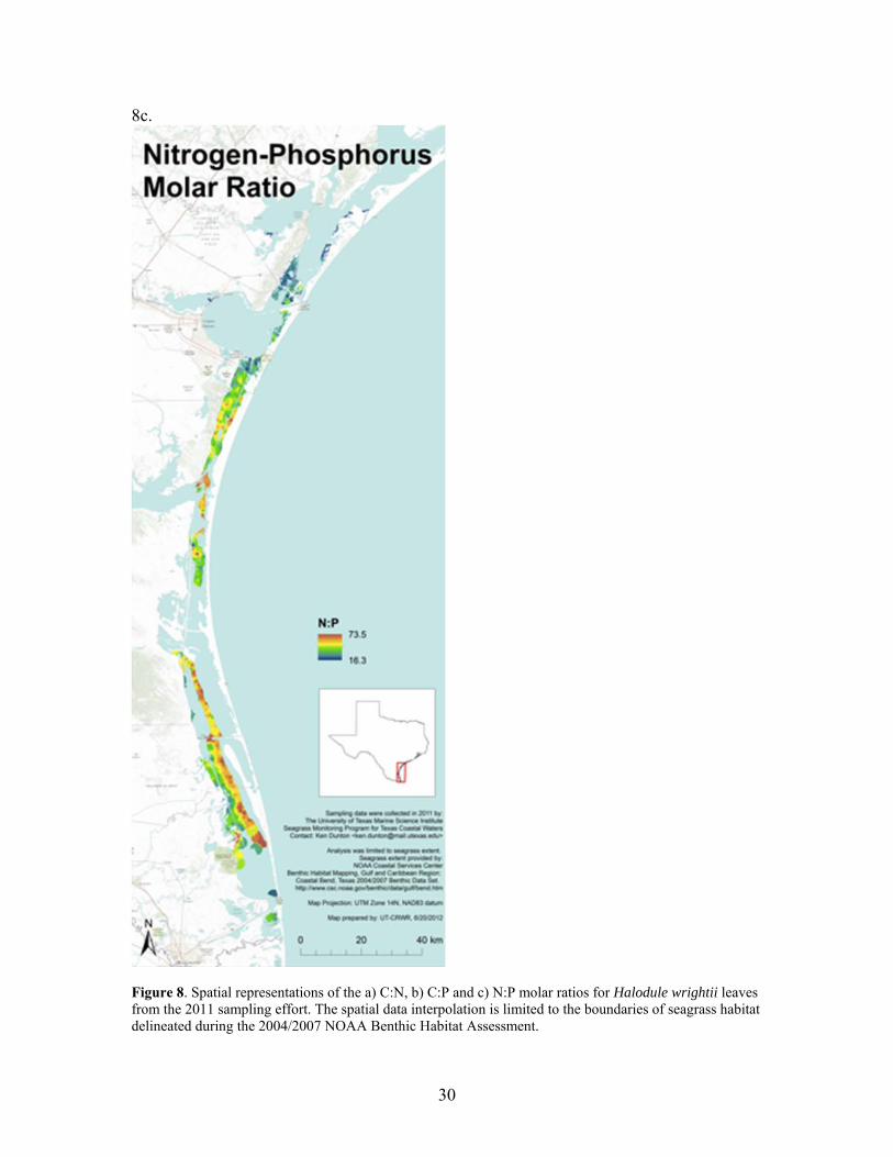
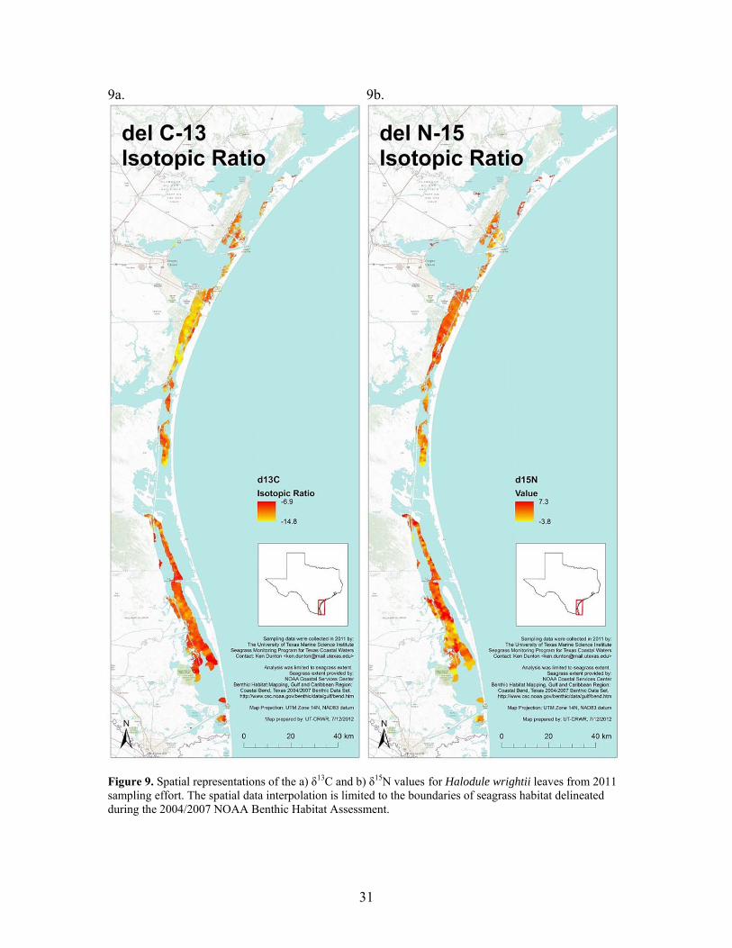
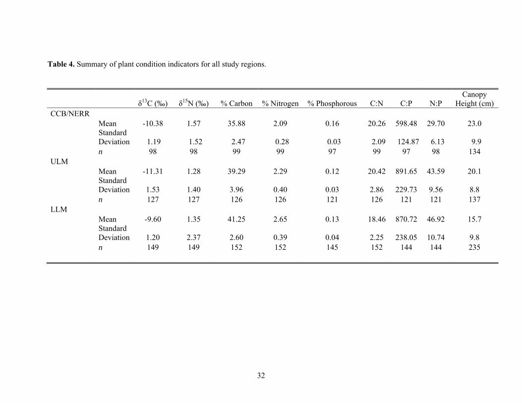
of all the sites (23.0 ± 9.9 cm; Table 4, Figure 6). The CCB/MANERR also exhibited the lowest mean percentage of leaf carbon (35.88 ± 2.47%; Table 4, Figure 7a) and nitrogen (2.09 ± 0.28%; Table 4, Figure 7b) and highest mean percentage of phosphorous (0.16 ± 0.03%; Table 4, Figure 7c) content. The high phosphorous content of seagrass leaves resulted in the lowest C:P (598.48 ± 124.87; Table 4, Figure 8b) and N:P (29.70 ± 6.13; Table 4, Figure 8c) ratios of any site. The ratio of C:N of seagrass leaves also varied the least spatially within the CCB/MANERR site (20.26 ± 2.09; Table 4, Figure 8a), was highest in Redfish Bay and lowest in eastern CCB. Lastly, this site exhibited an intermediate mean value of δ13C (-10.38 ± 1.19‰; Table 4, Figure 9a), but the most enriched δ15N (1.57 ± 1.52‰; Table 4, Figure 9b) value of any site.

Upper Laguna Madre

The ULM site contained the second highest and least variable canopy height of all

three sites (20.1 ± 8.8 cm; Table 4, Figure 6). This region exhibited the second highest mean percentage of leaf carbon (39.29 ± 3.96%; Table 4, Figure 7a), the most variable percentage of nitrogen (2.29 ± 0.40%; Table 4, Figure 7b) content and lowest mean percentage of phosphorous (0.12 ± 0.03%; Table 4, Figure 7c) content. The variable leaf nitrogen content resulted in the highest and most spatially variable C:N ratio (20.42 ± 2.86; Table 4, Figure 8a) of any site, while the low phosphorous content resulted in the highest mean C:P (891.65 ± 229.73; Table 4, Figure 8b) ratio of any site. Both the mean and standard deviation of the N:P (43.59 ± 9.56; Table 4, Figure 8c) ratio within the ULM region was in between the values recorded for the CCB/NERR and LLM regions. However, very high N:P (>55) ratios were recorded near the mouth of Baffin Bay. Lastly, the leaf tissue in this site possessed the most depleted δ13C (-11.31 ± 1.53‰; Table 4, Figure 9a) and δ15N (1.28 ± 1.40‰; Table 4, Figure 9b) values of any site.

Lower Laguna Madre

The LLM site contained the lowest mean canopy height of all three sites (15.7 ±

9.8 cm; Table 4, Figure 6), but contained tall seagrass canopies to the south near the Brazos Santiagos Pass. This site exhibited the highest mean percentages of leaf carbon (41.25 ± 2.60%; Table 4, Figure 7a) and nitrogen (2.65 ± 0.39%; Table 4, Figure 7b) and most spatially variable percentage of phosphorous (0.13 ± 0.04%; Table 4, Figure 7c) content. The high nitrogen content of seagrass leaves resulted in the lowest mean C:N

25

(18.46 ± 2.25; Table 4, Figure 8a) ratio and highest mean N:P (46.92 ± 10.74; Table 4, Figure 8c) ratio of any site, and the spatially variable phosphorous content translated into the most variable C:P (870.72 ± 238.04; Table 4, Figure 8b) and N:P ratios of any region. Lastly, the leaf tissue in the LLM possessed the most enriched mean δ13C (-9.60 ± 1.20‰; Table 4, Figure 9a) and most spatially variable δ15N (1.35 ± 2.37‰; Table 4, Figure 9b) values of any site, with a general depletion in δ15N values from north to south.

26

Figure 6. Spatial representation of seagrass canopy height from the 2011 sampling effort. The spatial data interpolation is limited to the boundaries of seagrass habitat delineated during the 2004/2007 NOAA Benthic Habitat Assessment.

27

7a. 7b.

28

7c.

Figure 7. Spatial representations of the percent a) carbon, b) nitrogen and c) phosphorous content of Halodule wrightii leaves from the 2011 sampling effort. The spatial data interpolation is limited to the boundaries of seagrass habitat delineated during the 2004/2007 NOAA Benthic Habitat Assessment.

29

8a. 8b.

30

8c.

Figure 8. Spatial representations of the a) C:N, b) C:P and c) N:P molar ratios for Halodule wrightii leaves from the 2011 sampling effort. The spatial data interpolation is limited to the boundaries of seagrass habitat delineated during the 2004/2007 NOAA Benthic Habitat Assessment.

31

9a. 9b.

Figure 9. Spatial representations of the a) δ13C and b) δ15N values for Halodule wrightii leaves from 2011 sampling effort. The spatial data interpolation is limited to the boundaries of seagrass habitat delineated during the 2004/2007 NOAA Benthic Habitat Assessment.

32

Table 4. Summary of plant condition indicators for all study regions.

δ13C (‰) δ15N (‰) % Carbon % Nitrogen % Phosphorous C:N C:P N:P Canopy

Height (cm) CCB/NERR

Mean -10.38 1.57 35.88 2.09 0.16 20.26 598.48 29.70 23.0 Standard Deviation 1.19 1.52 2.47 0.28 0.03 2.09 124.87 6.13 9.9 n 98 98 99 99 97 99 97 98 134

ULM Mean -11.31 1.28 39.29 2.29 0.12 20.42 891.65 43.59 20.1 Standard Deviation 1.53 1.40 3.96 0.40 0.03 2.86 229.73 9.56 8.8 n 127 127 126 126 121 126 121 121 137

LLM Mean -9.60 1.35 41.25 2.65 0.13 18.46 870.72 46.92 15.7 Standard Deviation 1.20 2.37 2.60 0.39 0.04 2.25 238.05 10.74 9.8 n 149 149 152 152 145 152 144 144 235

33

CONCLUSIONS

Water Quality The observed spatial pattern in salinity is likely attributed to the location of

navigational passes. There are four distinguishable connections to Gulf of Mexico throughout the study region (Aransas Pass, Packery Inlet, Port Mansfield Pass and Brazos Santiagos Pass). Higher salinities occurred in waters between consecutive passes that were not subject to regular tidal inflow from the comparably less saline waters of the Gulf of Mexico. Although areas near the passes had lower salinity, no clear salinity gradient existed from a pass to any lagoon midpoint. It is therefore not surprising that the ULM region, which does not contain a connection to the Gulf of Mexico, had the highest mean salinity. In contrast, both the CCB/MANERR and LLM regions contained large tidal passes and exemplified lower and similar salinity regimes.

It appears that salinity provides a reasonable descriptor of seagrass species

distributions in Texas coastal waters. For example, Halodule wrightii was observed in salinities ranging from 7-74 ppt. This is the largest documented salinity tolerance for any species encountered during this study and is likely influential in promoting its widespread distribution. To the contrary, Syringodium filiforme was only observed in salinities ranging from 38-52 ppt, which represents the smallest documented salinity tolerance of any species in this study. Furthermore, Syringodium filiforme was largely restricted to the hypersaline ULM site. It is therefore logical to hypothesize that Syringodium filiforme is unable to cope with large fluctuations in salinity, and is restricted to the ULM because of its high water residence time and low temporal salinity variation. Lastly, it appears that Thalassia testudinum (salinity range: 32-50 ppt) is restricted to areas in close proximity to tidal inlets, as the two largest distributions of this species were documented north of Aransas Pass and north of the Brazos Santiagos Pass. Both of these passes are capable of massive flushing events during tidal excursions, which serve to reduce water residence times and prevent extended periods of hypersalinity.

The spatial characteristics of dissolved oxygen were very similar to salinity.

Dissolved oxygen was lowest in the ULM and corresponded to areas of high salinity. In contrast, dissolved oxygen was highest in areas of lower salinity near tidal passes. It is likely that areas with high water residence times and salinities are not regenerated with oxygen-rich water from the Gulf of Mexico. As a result, the only sources of oxygen in these areas come from photosynthetic production and wave injection. It is important to note, however, that although the ULM had the lowest mean dissolved oxygen, this region also contained the highest mean cover of vegetation. It therefore does not appear that

34

lower dissolved oxygen concentrations are significantly impacting seagrass meadows within this region.

Water Transparency

During the 2011 sampling effort, the light environments of the CCB/MANERR

and ULM sites were remarkably similar (mean Kd: CCB/MANERR = 0.70 m-1; ULM = 0.73 m-1). The comparable Kd values are attributed to similar mean concentrations of TSS (CCB/MANERR= 13.72 mg L-1; ULM = 13.75 m L-1) and water column chlorophyll (CCB/MANERR= 5.31 ug L-1; ULM = 4.04 ug L-1). These Kd values suggest that seagrasses are capable of occupying depths greater than 2 m in these regions, based on light availability. However, it is important to note that chlorophyll concentrations were abnormally low in the ULM during this sampling effort, and persistent brown tides have been known to elevate chlorophyll concentrations to more than 20 μg L-1 within this region (Dunton, unpub. LM151 data). As a result, the low Kd values observed here are not long-term temporal averages and consequently are most useful for documenting spatial patterns in light attenuation, and likely overestimate actual seagrass depth limits.

The LLM site, which is largely influenced by the waters surrounding the Laguna

Atascosa Wildlife Refuge, exhibited an elevated and spatially variable mean light attenuation (Kd = 1.38 ± 0.97 m-1). In particular, the waters bordering this refuge contained extremely high concentrations of TSS (>100 mg L-1) and elevated concentrations of chlorophyll (>10 μg L-1). Given the observed light attenuation, it is not surprising that seagrasses were largely absent from this area. However, it is important to note that this area was designated as a seagrass habitat in the 2004/2007 NOAA Benthic Habitat Assessment. Currently, the ultimate source of the suspended solids and the magnitude of seagrass loss in this area remain unknown.

Seagrass Coverage and Species Distributions A total of five seagrass species were identified during the 2011 field sampling

effort (Halodule wrightii, Thalassia testudinum, Syringodium filiforme, Ruppia maritima and Halophila englemanii). Halodule wrightii was the most prevalent and widely distributed species encountered during the survey, and dominated the percent coverage in all three sites. Thalassia testudinum had the second highest abundance, but was largely absent from the ULM site. This species was most common near large tidal passes, which suggests that Thalassia testudinum prefers waters with low residence times. At this time, it is unclear if this preference is attributed to salinity tolerance, nutrient cycling or some

35

combination of variables. Although Syringodium filiforme was observed in all three sites, this species was most prevalent in the ULM region. Contrary to Thalassia testudinum, Syringodium filiforme was most abundant in waters with high residence times. Again, it is currently unknown whether Halodule wrightii and Thalassia testudinum are restricting Syringodium filiforme to the ULM waters through competitive exclusion in the MANERR, CCB and LLM sites, or if this species prefers some physical or chemical attribute of waters with high residence times. Lastly, this sampling effort documented small abundances of both Ruppia maritima and Halophila englemanii. The largest distribution of Ruppia maritima occurred south of Port Mansfield Pass in the LLM, while the largest distribution of Halophila englemanii occurred in the ULM near the northern boundaries of Padre Island National Seashore.

All three sites had a mean depth of less than 1 m, and no single station within a

site had water depths greater than 2 m. Since sampling stations were chosen based on seagrass distributions from previous remote sensing efforts, it is initially plausible to assume that seagrass plants in Texas coastal waters are restricted to depths less than 2 m. However, measurements of light attenuation suggest that seagrasses could potentially extend to deeper depths, as sufficient light (18% SI) extended to 2.44 m in the CCB/MANERR and 2.34 m in the ULM region. In support of this, we noted seagrasses at sampling stations which had depths greater than the mean water depth of 1 m.

Seagrass percent coverage was greatest in the ULM site followed by the

CCB/MANERR and LLM sites. It is currently difficult to determine whether seagrass meadows in Texas coastal waters are expanding or contracting, since this is the first comprehensive field assessment of seagrass coverage. However, assuming the 2004/2007 NOAA Benthic Habitat Assessment was an accurate delineation of seagrass habitat, it appears that seagrass meadows are currently in a state of decline. This conclusion is based on the fact that all three sites contained sampling stations without any vegetation, which ranged from 2.8% of all stations in the CCB/MANERR site to 17.2% of all stations in the LLM site. Many additional stations contained less than 10% of seagrass coverage, which ranged from 5.8% of all sampling stations in the CCB/MANERR site to 31.6% of all sampling stations in the LLM site. The high percentage of sampling stations with less than 10% seagrass coverage merits attention.

Plant Tissue Condition There was a notable decrease in mean canopy height from north to south along the

Texas coastline. The LLM exhibited the lowest mean canopy height and the lowest areal coverage of grasses for any site, which was consistent with the highest percentage of

36

nitrogen content, lowest mean C:N and highest mean N:P ratios for any site. In contrast, the highest mean canopy height was observed at the CCB/MANERR site, and this site also exhibited the highest mean percentage of phosphorous content and lowest mean C:P and N:P ratios of any site. These trends are quite interesting because seagrasses require both nitrogen and phosphorous for maintenance and growth. However, it appears that excess nitrogen is inhibiting seagrasses in the LLM, while an abundance of phosphorous is promoting shoot growth in the CCB/MANERR. These initial results suggest that molar C:N:P ratios of plant tissue constitute a reliable metric for assessing seagrass condition, but the physiological mechanisms relating nutrient supply to seagrass coverage require additional investigation.

The waters surrounding the land cut in the Laguna Madre generated interesting

plant tissue characteristics. The areas to the north and east of the land cut contained seagrasses with the highest C:N ratios and the most depleted δ15N values, while the waters surrounding the southern entrance of the land cut contained seagrasses with the lowest C:N ratios and the most enriched δ15N values. There are several possible mechanisms for the spatial patterns observed here. First, a significant nitrogen source may exist to the south of the land cut, which is resulting in the nitrogen enrichment of seagrass tissues. It is possible that shallow waters and land barriers would prevent this large amount of nitrogen from entering the interior portions of the Laguna Madre. Second, the depleted δ15N values and high C:N ratios also correspond to highly saline waters, and it is possible that tissue differences in the upper and lower Laguna Madre are actually attributed to water residence time and site-specific nitrogen availability. At this time, the relative importance of these two mechanisms remains unresolved.

37

FUTURE RECOMMENDATIONS

Tier 1

The current sampling regime relied heavily on past remote sensing efforts to

select the location of sampling stations. Unfortunately, the last comprehensive remote sensing effort was completed in 2007, which utilized, in part, 2004 imagery. Sampling station selection was consequently based on imagery that was already 4 to 7 years old at the time of sampling, and therefore may not accurately represent present-day seagrass distributions. For example, 17.2% of the sampling stations in the LLM site did not contain any vegetation and 31.6% of LLM sampling stations contained less than 10% seagrass coverage. Given the age of the remote sensing dataset, it is currently impossible to determine whether these values represent a significant decline in seagrass coverage or simply inadequate ground-truthing of the remote sensing imagery. Also, the 2004/2007 NOAA Benthic Habitat Assessment did not identify any seagrass coverage in areas greater than 2 m in depth. However, this study documented seagrass coverage throughout the deepest sampling stations (1.85 m depth), suggesting that other areas with greater depths may warrant attention. It is impossible to determine if seagrasses were truly absent in deeper waters during the 2004/2007 remote sensing effort, or if the imagery was incapable of identifying benthic vegetation in waters greater than 2 m deep. All of these shortcomings highlight the importance for more frequent remote sensing surveys that implement reliable ground-truthing protocols.

Tier 2

The 2011 sampling effort comprised 567 individual sampling stations and

successfully documented hydrographic parameters, seagrass coverage, species distributions and plant physiological condition along the South Texas coastline. This sampling effort provided a comprehensive examination of habitat quality indicators and developed the infrastructure required for a statewide Texas monitoring program. Permanent sampling stations were created using geospatial analysis and were shown to sufficiently elicit spatial patterns in measured parameters. The current project also developed a protocol for the organization of data and a website to make all of this information freely available to the public (www.TexasSeagrass.org). The protocols and data are easily accessible so that various state and federal agencies can utilize the resources developed here and, hopefully, achieve consistency amongst sampling efforts.

The effectiveness of the Tier 2 sampling program is highly dependent on the field

sampling schedule. In particular, this program utilizes a rapid sampling protocol that is

38

frequently repeated over a given area- the primary objective of this approach being to yield spatial relationships in measured parameters. However, this approach is not capable of capturing the temporal variability exhibited within a given system for any single metric. It is therefore imperative that the Tier 2 sampling program is repeated on a regular schedule (annual, biannual, etc.) in order to document spatial variability in habitat quality indicators through time and provide the most relevant information to resource managers.

Tier 3

One of the principle objectives of the Tier 2 sampling program is to identify areas

of concern through a suite of habitat quality indicators. The 2011 sampling effort successfully revealed such an area within the LLM site, in the waters surrounding the Laguna Atascosa Wildlife Refuge. This area was devoid of vegetation, and also corresponded with high light attenuation resulting from extremely high concentrations of TSS. Further research in a Tier 3 sampling program should specifically target the source of the particulate matter within the water column, monitor the underwater light environment through time, and determine if any other stressors (nutrients, epiphytes, etc.) contributed to the loss of seagrass habitat in the LLM.

39

REFERENCES

Chapman, H.D., Pratt, P.F., 1961. Methods of Analysis for Soils, Plants and Water. Univ. California, Berkeley, CA, USA.

Dennison, W.C., R.J. Orth, K.A. Moore, J.C. Stevenson, V. Carter, S. Kollar, P.W. Bergstrom, and R.A. Batiuk. 1993. Assessing Water Quality with Submersed Aquatic Vegetation. BioScience 43:86-94.

Dunton, K H., W. Pulich, Jr. and T. Mutchler. 2011. A seagrass monitoring program for Texas coastal waters. http://www.texasseagrass.org/. 39 pp.

Fourqurean, J.W., J.N. Boyer, M.J. Durako, L.N. Hefty, and B.J. Peterson. 2003. Forecasting responses of seagrass distributions to changing water quality using monitoring data. Ecological Applications 13:474-489.

Kirkman, H. 1996. Baseline and Monitoring Methods for Seagrass Meadows. Journal of Environmental Management 47:191-201.

Koch, E.W. 2001. Beyond light: Physical, geological, and geochemical parameters as possible submersed aquatic vegetation habitat requirements. Estuaries and Coasts 24:1-17.

Livingston, R.J., S.E. McGlynn, and N. Xufeng. 1998. Factors Controlling Seagrass Growth in a Gulf Coastal System: Water and Sediment Quality and Light. Aquatic Botany 60: 135-159.

Neckles, H.A., B.S. Kopp, B.J. Peterson, and P.S. Pooler. 2012. Integrating scales of seagrass monitoring to meet conservation needs. Estuaries and Coasts 35:23-46.

Pulich, W.M., Jr. and T. Calnan. (eds.) 1999. Seagrass Conservation Plan for Texas. Resource Protection Division. Austin, Texas: Texas Parks and Wildlife Department. 67 pp.

Pulich, W.M., Jr., B. Hardegree, A. Kopecky, S. Schwelling, C. P. Onuf, and K.H. Dunton. 2003. Texas Seagrass Monitoring Strategic Plan (TSMSP). Publ.Texas Parks and Wildlife Department, Resource Protection Division, Austin, Texas. 27 pp.

40

APPENDIX: METHODS

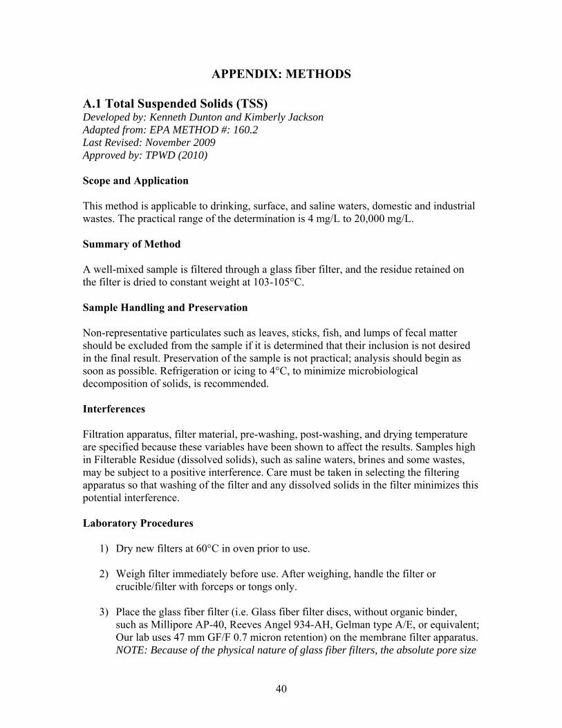
A.1 Total Suspended Solids (TSS) Developed by: Kenneth Dunton and Kimberly Jackson Adapted from: EPA METHOD #: 160.2 Last Revised: November 2009 Approved by: TPWD (2010) Scope and Application This method is applicable to drinking, surface, and saline waters, domestic and industrial wastes. The practical range of the determination is 4 mg/L to 20,000 mg/L. Summary of Method A well-mixed sample is filtered through a glass fiber filter, and the residue retained on the filter is dried to constant weight at 103-105°C. Sample Handling and Preservation Non-representative particulates such as leaves, sticks, fish, and lumps of fecal matter should be excluded from the sample if it is determined that their inclusion is not desired in the final result. Preservation of the sample is not practical; analysis should begin as soon as possible. Refrigeration or icing to 4°C, to minimize microbiological decomposition of solids, is recommended. Interferences Filtration apparatus, filter material, pre-washing, post-washing, and drying temperature are specified because these variables have been shown to affect the results. Samples high in Filterable Residue (dissolved solids), such as saline waters, brines and some wastes, may be subject to a positive interference. Care must be taken in selecting the filtering apparatus so that washing of the filter and any dissolved solids in the filter minimizes this potential interference. Laboratory Procedures

1) Dry new filters at 60°C in oven prior to use.

2) Weigh filter immediately before use. After weighing, handle the filter or crucible/filter with forceps or tongs only.

3) Place the glass fiber filter (i.e. Glass fiber filter discs, without organic binder, such as Millipore AP-40, Reeves Angel 934-AH, Gelman type A/E, or equivalent; Our lab uses 47 mm GF/F 0.7 micron retention) on the membrane filter apparatus. NOTE: Because of the physical nature of glass fiber filters, the absolute pore size

41

cannot be controlled or measured. Terms such as “pore size”, “collection efficiencies” and “effective retention” are used to define this property in glass fiber filters.

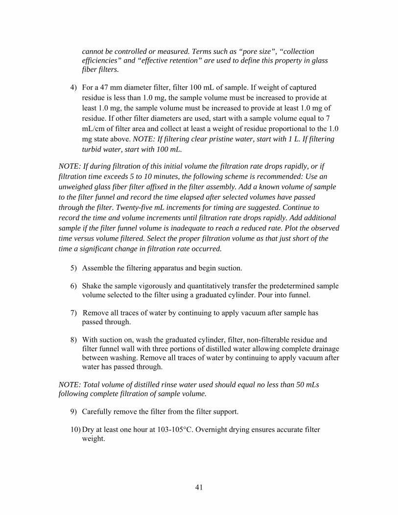
4) For a 47 mm diameter filter, filter 100 mL of sample. If weight of captured residue is less than 1.0 mg, the sample volume must be increased to provide at least 1.0 mg, the sample volume must be increased to provide at least 1.0 mg of residue. If other filter diameters are used, start with a sample volume equal to 7 mL/cm of filter area and collect at least a weight of residue proportional to the 1.0 mg state above. NOTE: If filtering clear pristine water, start with 1 L. If filtering turbid water, start with 100 mL.

NOTE: If during filtration of this initial volume the filtration rate drops rapidly, or if filtration time exceeds 5 to 10 minutes, the following scheme is recommended: Use an unweighed glass fiber filter affixed in the filter assembly. Add a known volume of sample to the filter funnel and record the time elapsed after selected volumes have passed through the filter. Twenty-five mL increments for timing are suggested. Continue to record the time and volume increments until filtration rate drops rapidly. Add additional sample if the filter funnel volume is inadequate to reach a reduced rate. Plot the observed time versus volume filtered. Select the proper filtration volume as that just short of the time a significant change in filtration rate occurred.

5) Assemble the filtering apparatus and begin suction.

6) Shake the sample vigorously and quantitatively transfer the predetermined sample volume selected to the filter using a graduated cylinder. Pour into funnel.

7) Remove all traces of water by continuing to apply vacuum after sample has

passed through.

8) With suction on, wash the graduated cylinder, filter, non-filterable residue and filter funnel wall with three portions of distilled water allowing complete drainage between washing. Remove all traces of water by continuing to apply vacuum after water has passed through.

NOTE: Total volume of distilled rinse water used should equal no less than 50 mLs following complete filtration of sample volume.

9) Carefully remove the filter from the filter support.

10) Dry at least one hour at 103-105°C. Overnight drying ensures accurate filter weight.

42

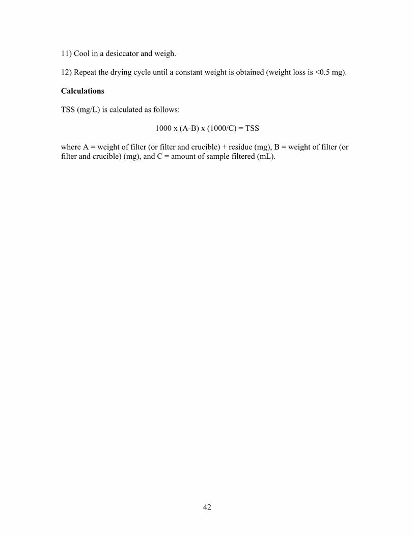
11) Cool in a desiccator and weigh. 12) Repeat the drying cycle until a constant weight is obtained (weight loss is <0.5 mg). Calculations TSS (mg/L) is calculated as follows:

1000 x (A-B) x (1000/C) = TSS

where A = weight of filter (or filter and crucible) + residue (mg), B = weight of filter (or filter and crucible) (mg), and C = amount of sample filtered (mL).

43

A.2 Percent Surface Irradiance (% SI) and Light Attenuation (k) Developed by: Kenneth Dunton and Kimberly Jackson Last Revised: December 2009 Approved by: EPA (2002) and TPWD (2010) Field Procedures Measurements of percent surface irradiance (% SI) and the diffuse light attenuation coefficient (k) are made from simultaneous measurements of surface (ambient) and underwater irradiance. Surface measurements of photosynthetically active radiation (PAR = ca. 400 to 700 nm wavelength) are collected using an LI-190SA quantum sensor that provides input to a LI-1000 datalogger (LI-COR Inc., Lincoln, Nebraska, USA). Underwater measurements are made using a LI-192SA or LI-193SA spherical quantum sensor. Measurements of % SI and k are based on three or more replicate determinations of instantaneous PAR collected by the surface and underwater sensors and recorded by the LI-1000 datalogger. Care is taken to reduce extraneous sources of reflected light (from boats or clothing). Calculations Percent surface irradiance available at the seagrass canopy is calculated as follows:

% SI = (Iz/I0) x 100 where Iz and I0 are irradiance (µmol photons m-2s-1) at depth z (meters) and at the surface, respectively. Light attenuation is calculated using the transformed Beer-Lambert equation:

kd = -[ln(Iz/I0)]/z where k is the attenuation coefficient (m-1) and Iz and I0 are irradiance (µmol photons m-2 s-1) at depth z (meters) and at the surface, respectively.

44

A.3 Seagrass Tissue Nutrient and Isotopic Analysis Developed by: Kenneth Dunton, Kimberly Jackson, Christopher Wilson, Karen Bishop and Sang Rul Park Last Revised: December 2009 Approved by: EPA (2002) and TPWD (2010) Tissue Preparation Newly formed leaves (the youngest leaf in a shoot bundle) are gently scraped and rinsed in tap water to remove algal and faunal epiphytes. The rinsed tissue samples are then dried to a constant weight at 60°C and homogenized by grinding to a fine powder using a mortar and pestle. The same sample is used for both C:N and P calculations. Tissue C:N Content, δ13C and δ15N Tissue samples are analyzed for carbon and nitrogen concentrations and isotopic values using either a PDZ Europa ANCA-GSL elemental analyzer coupled to a PDZ Europa 20-20 isotope ratio mass spectrometer (UC-Davis; precision 0.2 ‰ for 13C and 0.3 ‰ for 15N), or a Carlo Erba 2500 elemental analyzer coupled to a Finnigan MAT DELTAplus isotope ratio mass spectrometer 23 (UTMSI; precision 0.3 ‰ for both 13C and 15N). Tissue Phosphorous Content Required Reagents

A. Ammonium Heptamolybdate-Ammonium Vanadate in Nitric Acid

1) Dissolved Dissolve 22.5 g ammonium heptamolybdate [(NH4)6Mo7O24. 4H2O] in 400 mL DW (a).

2) Dissolve 1.25 g ammonium metavanadate (NH4VO3) in 300 mL hot DW (b).

3) Add (b) to (a) in a 1 L volumetric flask, and let the mixture cool to room temperature.

4) Slowly add 250 mL concentrated nitric acid (HNO3) to the mixture, cool the solution to room temperature, and bring to 1 L volume with DW.

B. Acid Mixture for Tissue Digestion

1) Dilute 165.6 mL concentrated hydrochloric acid (HCl, 37%, sp.gr.1.19) in DW, mix well, let cool, and bring to 1 L volume with DW (2N HCl).

45

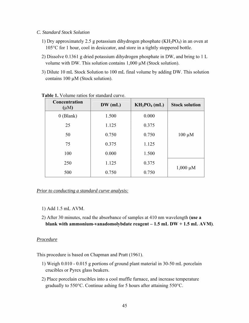
C. Standard Stock Solution

1) Dry approximately 2.5 g potassium dihydrogen phosphate (KH2PO4) in an oven at 105°C for 1 hour, cool in desiccator, and store in a tightly stoppered bottle.

2) Dissolve 0.1361 g dried potassium dihydrogen phosphate in DW, and bring to 1 L volume with DW. This solution contains 1,000 µM (Stock solution).

3) Dilute 10 mL Stock Solution to 100 mL final volume by adding DW. This solution contains 100 µM (Stock solution).

Table 1. Volume ratios for standard curve. Concentration

(µM) DW (mL) KH2PO4 (mL) Stock solution

0 (Blank) 1.500 0.000

100 µM

25 1.125 0.375

50 0.750 0.750

75 0.375 1.125

100 0.000 1.500

250 1.125 0.375 1,000 µM

500 0.750 0.750

Prior to conducting a standard curve analysis:

1) Add 1.5 mL AVM.

2) After 30 minutes, read the absorbance of samples at 410 nm wavelength (use a blank with ammonium-vanadomolybdate reagent – 1.5 mL DW + 1.5 mL AVM).

Procedure

This procedure is based on Chapman and Pratt (1961).

1) Weigh 0.010 - 0.015 g portions of ground plant material in 30-50 mL porcelain crucibles or Pyrex glass beakers.

2) Place porcelain crucibles into a cool muffle furnace, and increase temperature gradually to 550°C. Continue ashing for 5 hours after attaining 550°C.

46

3) Shut off the muffle furnace and open the door cautiously for rapid cooling. When cool, carefully remove the porcelain crucibles.

4) Dissolve the cooled ash in 1 mL portions 2 N hydrochloric acid (HCl) and mix with a plastic rod.

5) After 15-20 minutes, add 4 mL DW.

6) Mix thoroughly, allow to stand for approximately 30 minutes, and use the supernatant or filter through Whatman No. 42 filter paper, discarding the first portions of the filtrates (optional).

Measurements

1) Pipette 1.5 mL of the digest filtrate or aliquot of the dissolved ash (depending on the procedure used) into a 15 mL glass tube, then add 1.5 mL ammonium-vanadomolybdate reagent.

2) After 30 minutes, read the absorbance of samples at 410 nm wavelength (use a blank with ammonium-vanadomolybdate reagent – 1.5 mL DW + 1.5 mL AVM).

3) Prepare a calibration curve for standards, plotting absorbance against the respective P concentrations

4) Read P concentrations in the unknown samples from the calibration curve. Calculations Total phosphorus in plant (%P) =

C (µmol/L) x (1 L/1,000 mL) x 5 mL x (30.9738 µg/µmol) x (1 g/1,000,000 µg) x (1/g sample)

when 5 mL = total volume of the digest/aliquot (In this method, total volume is 5 mL (1 mL of 2 N HCl + 4 mL of DW)), and g sample = weight of dry plant used (g).

Reference

Chapman, H.D. and Pratt, P.F. 1961. Methods of Analysis for Soils, Plants and Water. Univ. California, Berkeley, CA, USA.