Assessment of Seismic Risk for Subsea Production … of Seismic Risk for Subsea Production Systems in the Gulf of Mexico by Laura Ann Brown, M.S., Texas A&M University Joseph M. Bracci,

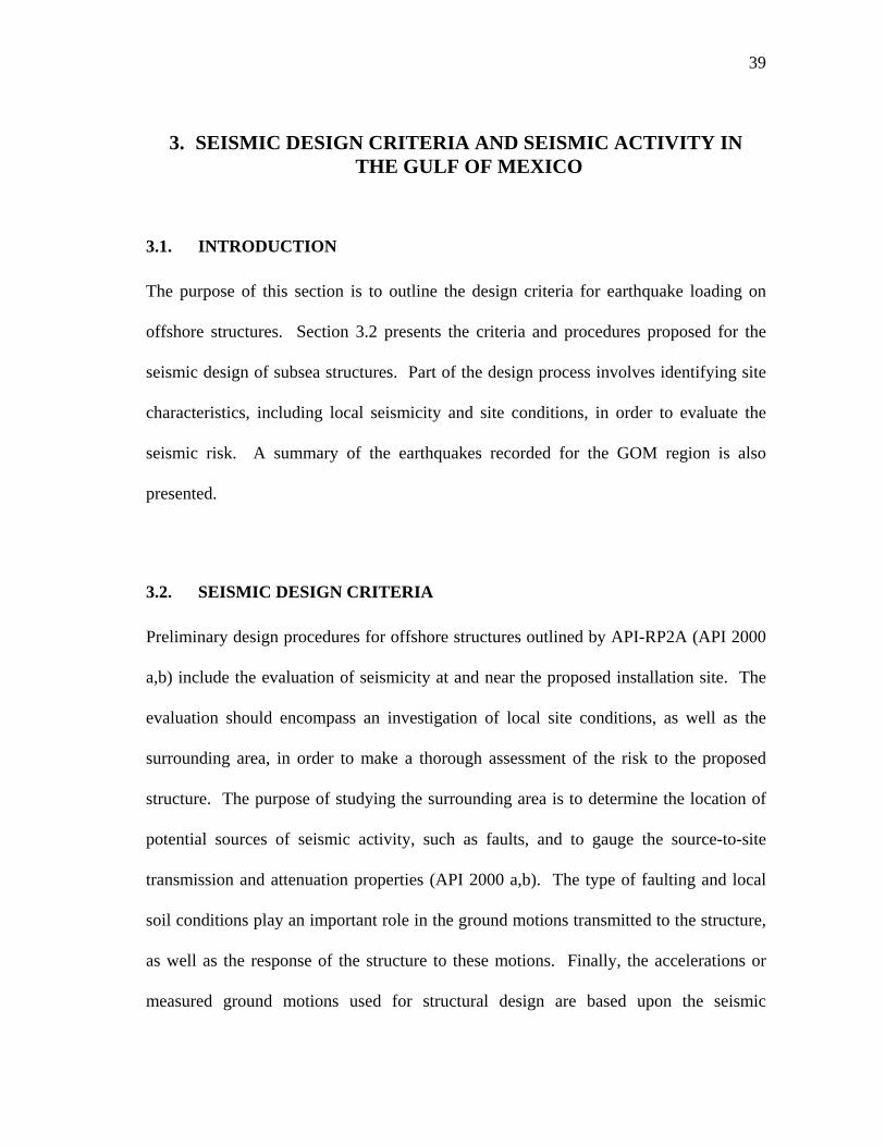
Assessment of Seismic Risk for Subsea Production Systems in the Gulf of Mexico

by

Laura Ann Brown, M.S., Texas A&M University Joseph M. Bracci, Mary Beth Hueste, J. Don Murff, Texas A&M University

Final Project Report Prepared for the Minerals Management Service Under the MMS/OTRC Cooperative Research Agreement

1435-01-99-CA-31003 Task Order 18204

Project Number 422

December 2003

OTRC Library Number: 12/03A136

Fo

Offshor

Colle

OffshorThe

1A

A National Science

“The views and conclusions contained in this document are those of the authors and should not be interpreted as representing the opinions or policies of the U.S. Government. Mention of trade names or commercial products does not constitute their endorsement by the U. S. Government”.

r more information contact:

e Technology Research Center Texas A&M University

1200 Mariner Drive ge Station, Texas 77845-3400

(979) 845-6000

or

e Technology Research Center University of Texas at Austin University Station C3700 ustin, Texas 78712-0318

(512) 471-6989

Foundation Graduated Engineering Research Center

ii

ABSTRACT

The number of subsea production systems placed in deepwater locations in the Gulf of

Mexico (GOM) has increased significantly in the last ten to fifteen years. Currently,

API-RP2A (2000 a,b) designates the GOM as a Zone 0 seismic risk area, indicating

an area of low seismic activity with an expected horizontal ground motion of less than

0.05g, and thus does not require seismic effects to be considered during the design process.

However, there have been a number of seismic events with Richter magnitudes between 3.0

and 4.9 that have occurred in this region. As a result, questions have been raised regarding

the seismic performance of deepwater subsea systems.

This study presents an analytical parametric study where a prototype subsea structure

was selected based on a survey of subsea systems. The baseline analytical model

consisted of a single casing embedded in soft clay soils, which supported a lumped mass

at a cantilevered height above the soil. A number of the model characteristics were

varied in the parametric study to simulate the structural response of a range of subsea

structures. This study examined the impact of API-RP2A Zone 1 and 2 design seismic

demands for the performance of subsea structures to provide a conservative bound for

the performance of a Zone 0 area such as the Gulf of Mexico. The results from the

subsequent analyses show that the stresses and deflections produced by the Zone 1 and

2 peak ground accelerations fall within the allowable design limits.

Debbie Oakes

Note

Accepted set by Debbie Oakes

Debbie Oakes

Note


Debbie Oakes

Note


Debbie Oakes

Note


Debbie Oakes

Note


iii

TABLE OF CONTENTS

Page

ABSTRACT ................................................................................................................. ii

TABLE OF CONTENTS ............................................................................................ iii

LIST OF FIGURES...................................................................................................... vi

LIST OF TABLES ....................................................................................................... x

1. INTRODUCTION .................................................................................................... 1

1.1. Background ...................................................................................................... 1 1.2. Objectives and Methodology ........................................................................... 4 1.3. Thesis Outline .................................................................................................. 8

2. LITERATURE REVIEW ......................................................................................... 9

2.1. Introduction ...................................................................................................... 9 2.2. Modeling and Analysis..................................................................................... 9

2.2.1. General .................................................................................................. 9 2.2.2. Hydrodynamic Effects........................................................................... 12 2.2.3. Forces Due to Waves and Currents ....................................................... 14 2.2.4. Soil-Casing Interaction for Soft Clays .................................................. 15 2.2.5. Spectral Analysis Method ..................................................................... 19 2.2.6. Time History Analysis .......................................................................... 23

2.3. Previous Seismic Research of Offshore Systems.............................................. 24 2.3.1. Offshore Ground Motions ..................................................................... 24 2.3.2. Seismic Analysis of Fixed Platforms .................................................... 27 2.3.3. Pile Behavior Under Seismic Loading .................................................. 31 2.3.4. Subsea Pipelines Under Seismic Loading............................................. 34 2.3.5. Conclusion............................................................................................. 37

3. SEISMIC DESIGN CRITERIA AND SEISMIC ACTIVITY IN THE GULF OF MEXICO................................................................................................................... 39

3.1. Introduction ....................................................................................................... 39 3.2. Seismic Design Criteria..................................................................................... 39 3.2. Seismicity of the Gulf of Mexico...................................................................... 42

4. SUBSEA SYSTEMS ................................................................................................ 48

4.1. Introduction ....................................................................................................... 48 4.2. Overview of Subsea Systems ............................................................................ 48

iv

Page

4.2.1. General .................................................................................................. 48 4.2.2. Wellhead Completion Equipment ......................................................... 49 4.2.3. Templates ............................................................................................. 52 4.2.4. Manifold Systems................................................................................. 54 4.2.5. Subsea Systems in the Gulf of Mexico ............................................... 55

5. STRUCTURAL MODELS AND ANALYSIS PROCEDURES............................. 60

5.1. Introduction ..................................................................................................... 60 5.2. Description of Analytical Model..................................................................... 60

5.2.1. Prototype Structure............................................................................... 60 5.2.2. Baseline Analytical Model ................................................................... 62 5.2.3. Modeling Parameters............................................................................ 67 5.2.4. Details of the Time History Analysis Model ....................................... 70

5.3. Analysis Procedures ........................................................................................ 72 5.3.1. General ................................................................................................. 72 5.3.2 Calculation of Equivalent Soil-Casing Stiffness................................. 73 5.3.3. Time History Analysis Method ............................................................ 79 5.3.4. Calculation of Force and Stress Values................................................ 79

6. ANALYTICAL RESULTS ..................................................................................... 84

6.1. Introduction ..................................................................................................... 84 6.2. Parametric Study ............................................................................................. 84

6.2.1. Results for the Baseline Model ............................................................ 84 6.2.2. Variation of Soil-Casing Stiffness........................................................ 85 6.2.3. Variation of Casing Size ...................................................................... 90 6.2.4. Variation of Mudline Strength and Strength Gradient of the Soil ....... 94 6.2.5. Variation of Mass Height Above the Mudline ..................................... 101 6.2.6. Variation of Mass ................................................................................. 105 6.2.7. Variation of Mass and Mass Height Above the Mudline..................... 109 6.2.8. Fixity Variation .................................................................................... 114 6.2.9. Summary of Parametric Study Results................................................. 118

6.3. Time History Analysis Results........................................................................ 126 6.4. Conclusion....................................................................................................... 130

7. SUMMARY AND CONCLUSIONS ...................................................................... 131

7.1. Summary ......................................................................................................... 131 7.2. Conclusions ..................................................................................................... 133 7.3. Recommendations ........................................................................................... 135

REFERENCES............................................................................................................. 136

APPENDIX A. SAMPLE CALCULATIONS............................................................. 143

v

Page

A.1. Introduction ..................................................................................................... 143 A.2. Calculation of Input Values for BMCOL 76................................................... 143 A.3. Calculation of Soil-Casing Stiffness ............................................................... 145 A.4. Calculation of Stresses and Displacements..................................................... 147

vi

LIST OF FIGURES FIGURE Page 2.1. Simplified Structural Model..................................................................................... 10 2.2. Response Spectra, El Centro Earthquake, May 18, 1940 (Newmark and Hall

1987)......................................................................................................................... 20 2.3. Design Spectra Taken from API-RP2A (API 2000 a,b) ......................................... 23 2.4. Elevation View of Model Platform for Ground Motion Comparison Study

(Smith 1997)............................................................................................................. 26 2.5. Illustration of Computer Model F (Boote et al. 1998) ............................................. 30 2.6. Impact of Earthquake Magnitude and Proximity on Pipeline (Jones 1985) ............ 35 3.1. API-RP2A Seismic Risk of Map of Coastal Waters in Contiguous United States

(API 2000 a,b) .......................................................................................................... 42 3.2. Recorded Earthquakes in GOM Region and Bay of Campeche Region (Latitude

Range 18°- 32° and Longitude Range -98° to -82°) ................................................ 45 4.1. Subsea Wellhead System (API 1996) ...................................................................... 49 4.2. Tubing Hangar Installation (API 1996) ................................................................... 51 4.3. Subsea Completion Loads and Reactions (API 1996) ............................................. 51 4.4. Diagram of Well Spacer/Support Template (API 1996) .......................................... 52 4.5. Deepwater Subsea Systems and Recorded Earthquake Epicenters in the Gulf of

Mexico...................................................................................................................... 57 4.6. Gemini Subsea Development (Beer and Jeffries 2000) ........................................... 58 4.7. Zinc Template/Manifold – Elevation (Bednar 1993)............................................... 59 5.1. Advertisement for Kvaerner Subsea Christmas Tree (Kvaerner 2001) ................... 62 5.2. Free-Headed and Fixed-Headed Analytical Models ................................................ 63

vii

FIGURE Page 5.3. Lumped Mass Model for Time History Analysis..................................................... 71 5.4. 1940 El Centro, California Earthquake Acceleration Record (COSMOS 2003) ..... 72 5.5. Force Versus Displacement Curve ........................................................................... 76 5.6. API Design Spectra (API 2000 a,b) ......................................................................... 78 6.1. Change in Period Due to Variation of Soil-Casing Stiffness .................................... 88 6.2. Change in Displacement Due to Variation of Soil-Casing Stiffness......................... 88 6.3. Change in Shear Stress Due to Variation of Soil-Casing Stiffness........................... 89 6.4. Change in Bending Stress Due to Variation of Soil-Casing Stiffness ...................... 89 6.5. Change in Period Due to Variation of Casing Size ................................................... 92 6.6. Change in Deflections Due to Variation of Casing Size ........................................... 92 6.7. Change in Shear Stress Due to Variation of Casing Size.......................................... 93 6.8. Change in Bending Stress Due to Variation of Casing Size ..................................... 93 6.9. Change in Period Due to Variation of Mudline Strength.......................................... 97 6.10. Change in Deflection Due to Variation of Mudline Strength ................................. 97 6.11. Change in Shear Stress Due to Variation of Mudline Strength............................... 98 6.12. Change in Bending Stress Due Variation of Mudline Strength .............................. 98 6.13. Change in Period Due to Variation of Strength Gradient ....................................... 99 6.14. Change in Deflection Due to Variation of Strength Gradient ................................. 99 6.15. Change in Shear Stress Due to Variation of Strength Gradient ............................ 100 6.16. Change in Bending Stress Due Variation of Strength Gradient............................ 100 6.17. Change in Period Due to Variation of Mass Height.............................................. 103

viii

FIGURE Page 6.18. Change in Displacement Due to Variation of Mass Height .................................. 103 6.19. Change in Shear Stress Due to Variation of Mass Height .................................... 104 6.20. Change in Bending Stress Due to Variation of Mass Height ................................ 104 6.21. Change in Period Due to Variation of Mass.......................................................... 107 6.22. Change in Displacement Due to Variation of Mass .............................................. 107 6.23. Change in Shear Stress Due to Variation of Mass ................................................ 108 6.24. Change of Bending Stress Due to Variation of Mass............................................ 108 6.25. Change in Period Due to Variation of Mass and Height....................................... 112 6.26. Change in Displacement Due to Variation of Mass and Height ........................... 112 6.27. Change in Shear Stress Due to Variation of Mass and Height.............................. 113 6.28. Change in Bending Stress Due to Variation of Mass and Height ......................... 113 6.29. Comparison of Period Values Obtained from Free-Headed and Fixed-Headed Casings........................................................................................... 116 6.30. Comparison of Displacement Values Obtained from Free-Headed and Fixed-Headed Casings........................................................................................... 116 6.31. Comparison of Shear Stress Values Obtained from Free-Headed and Fixed- Headed Casings ..................................................................................................... 117 6.32. Comparison of Bending Stress Values Obtained from Free-Headed and Fixed-Headed Casings........................................................................................... 117 6.33. Range of Period Values for Parameter Variations – Free Headed Pile................. 119 6.34. Range of Maximum Displacement Values for Parameter Variations ................... 122 6.35. Range of Shear Stress Values for Parameter Variations. ...................................... 124 6.36. Range of Bending Stress Values for Parameter Variations................................... 126

ix

FIGURE Page 6.37. Acceleration Record from 1940 El Centro, CA Earthquake ................................ 128 6.38. Response Spectra and API Design Spectra ........................................................... 128 6.39. Accelerations Obtained from Time History Analysis ........................................... 129 6.40. Shear Forces Obtained from Time History Analysis ............................................ 129 A.1. Force-Displacement Curve for Baseline Analytical Model ................................... 146 A.2. Zone 1 Casing Displacement Profile...................................................................... 150 A.3. Zone 2 Casing Displacement Profile...................................................................... 150 A.4. Zone 1 Casing Shear Profile................................................................................... 151 A.5. Zone 2 Casing Shear Profile................................................................................... 151 A.6. Zone 1 Casing Moment Profile .............................................................................. 152 A.7. Zone 2 Casing Moment Profile .............................................................................. 152

x

LIST OF TABLES

TABLE Page

3.1. Recorded Earthquakes in the Gulf of Mexico Region (Latitude Range 20° to 32° and Longitude Range -98° to -82°) (USGS 2003)........................................ 43

3.2. Recorded Earthquakes in Bay of Campeche Region (Latitude Range 18°

to 20° and Longitude Range -98° to -90°) (USGS 2003)........................................ 44 4.1. Dimensions and Weights of Modules (Goodfellow Associates 1990) .................... 53 4.2. Partial Listing of Some Deepwater Subsea Systems Located in GOM ................... 56 5.1. Characteristics of the Baseline Analytical Model .................................................... 64 5.2. Loadings and Stresses Due to Current with Specified Velocities............................ 67 5.3. Variation of Range of Soil-Casing Stiffness ............................................................ 68 5.4. Variation of Casing Size .......................................................................................... 69 5.5. Variation of Mudline Strength ................................................................................. 69 5.6. Variation of Strength Gradient................................................................................. 69 5.7. Variation of Mass and Height .................................................................................. 70 5.8. Variations for Fixed-Headed Casing Models........................................................... 70 5.9. Values of p-y Curve for Soft Clays (API 2000 a,b) ................................................. 74 6.1. Baseline Model (CC) Results................................................................................... 85 6.2. Response Spectra Calculations for Variation of Soil-Casing Stiffness..................... 87 6.3. Force and Stress Values for Variation of Soil-Casing Stiffness ............................... 87 6.4. BMCOL76 and Response Spectra Calculations for Variations of Casing Size ........ 91 6.5. Resulting Force and Stress Values for Variation of Casing Size .............................. 91

xi

TABLE Page

6.6. BMCOL76 and Response Spectra Calculations for Variation of Mudline Strength ..................................................................................................................... 95 6.7. Force and Stress Values for Variation of Mudline Strength ..................................... 95 6.8. BMCOL76 and Response Spectra Calculations for Variation of Strength Gradient ..................................................................................................................... 96 6.9. Force and Stress Values for Variation of Strength Gradient..................................... 96 6.10. BMCOL76 and Response Spectra Calculations for Variation of Mass Height .... 102 6.11. Resulting Force and Stress Values for Height Variations..................................... 102 6.12. BMCOL 76 and Response Spectra Calculations for Variation of Mass ............... 106 6.13. Force and Stress Values for Variation of Mass..................................................... 106 6.14. BMCOL76 and Response Spectra Calculations for Variation of Mass and Height .................................................................................................................... 110 6.15. Force and Stress Values for Variation of Mass and Height .................................. 111 6.16. BMCOL76 and Response Spectra Calculations for Fixed-Headed Casing .......... 115 6.17. Force and Stress Values for Fixed-Headed Casing ............................................... 115 6.18. Summary of Results for Parameter Variation ....................................................... 118 6.19. Summary of Period Data from Parametric Study – Fixed-Headed Pile................. 119 6.20. Summary of Period Data from Parametric Study – Free-Headed Pile.................. 120 6.21. Summary of Deflection Data from Parametric Study – Free-Headed Pile ........... 121 6.22. Summary of Deflection Data from Parametric Study – Fixed-Headed Pile .......... 122 6.23. Summary of Shear Stresses from Parametric Study – Free-Headed Pile............... 123

xii

TABLE Page

6.24. Summary of Shear Stresses from Parametric Study – Fixed-Headed Pile............. 124 6.25. Summary of Bending Stresses from Parametric Study – Free-Headed Pile ......... 125 6.26. Summary of Bending Stresses from Parametric Study – Fixed-Headed Pile ........ 126 6.27. Time History Analysis Results (SAP2000 1999).................................................. 127 A.1. Required Soil and Casing Properties for BMCOL76 Analysis.............................. 144 A.2. P-y Curve Values for Soft Clays (API 2000 a,b) ................................................... 144 A.3. Lateral Soil Resistance Properties for BMCOL76 Input ....................................... 145 A.4. Deflections Obtained from BMCOL76.................................................................. 146 A.5. Soil-Casing Calculations for Zone 1 ...................................................................... 147 A.6. Soil-Casing Calculations for Zone 2 ..................................................................... 147 A.7. Summary of Results from Soil-Casing Calculations.............................................. 147 A.8. Summary of Displacement and Stress Results ....................................................... 149

1

1. INTRODUCTION

1.1. BACKGROUND

The use of subsea systems at deep water sites in the Gulf of Mexico has become

increasing popular in recent years due to the growing demand for energy and

continuing advances in the construction, placement and maintenance of subsea

systems (Deluca 2002). With this increase, questions have been raised about the

performance of these deep water subsea systems during earthquakes. The potential

vulnerabilities of subsea systems during earthquakes are created by the earthquake

shaking itself, liquefaction potential, and dynamic impact from soil sliding due to

nearby slope instability. The focus of this research is to evaluate the shaking

performance of subsea systems placed in deep water environments in the Gulf of

Mexico during potential earthquakes.

Historically, the Gulf of Mexico (GOM) has played a key role in providing energy

resources for the United States. Even as the exploration and development of other

regions has slowed, the GOM continues to see new construction throughout the

region. In addition, the technological advances in the construction, placement, and

maintenance of offshore structures have kept pace with the increasing demand for

energy. These advances have provided energy companies with a means of producing

This report follows the style and format of the ASCE Journal of Structural Engineering.

2

oil and gas from sites which were previously inaccessible because of their extreme

water depths. Critical improvements in technology include the development of

subsea systems capable of retrieving and pre-processing oil and gas at sites located

miles away from the host platform. As a result, resources can be accessed at sites

where the expected production, water depth, or other conditions would not justify the

construction of a platform.

As companies employ new technologies in order to extend developments out into

deeper waters, it is important to assess their seismic adequacy. For this reason,

research in areas such as seabed technology and deepwater construction is necessary

to study their seismic performance. The Minerals Management Service funded

several projects that researched different aspects of offshore systems in deepwater

environments (Smith 1997).

Currently, the use of these deep water systems is primarily concentrated in the

eastern GOM, south of Louisiana. A few examples of these developments include

Gemini, Zinc, Mensa, and Canyon Express. The Gemini development is located at a

water depth of approximately 1040 m at a site 145 km southeast of New Orleans

(Coleman and Isenmann 2000). Zinc is located in the Mississippi Canyon in 445 m

of water at a site with highly unconsolidated soil (Bednar 1993). Also located in the

Mississippi Canyon, at a water depth of 1615 m, Mensa consists of a manifold with a

template base set on the seafloor (McLaughlin 1998). To date, one of the deepest

Debbie Oakes

Note


3

subsea tiebacks is Canyon Express (extending through the Mississippi and Desoto

Canyon areas), which and collects and transports gas from fields with depths ranging

from 2015 to 2215 m (Deluca 2002).

One of the controlling factors in the design of offshore structures is the effect of

environmental loads due to wave, current, wind and geologic activity. According to

the American Petroleum Institute (API) in document API-RP2A (API 2000 a,b);

earthquake shaking, fault movement, and sea floor instability are all geologic

processes that must be accounted for in the design. Because subsea systems are

located directly on the seafloor, the processes mentioned above could play an important

role in the design and placement of these systems. The focus of this research is

directed exclusively toward the evaluating the performance of subsea systems during

potential earthquake shaking.

API outlines the loads to be considered for the design of subsea structural systems in

RP17A (API 1996) and RP2A (API 2000 a,b). These loads include gravity loads,

externally applied loads caused by risers or pipelines, thermal stresses, and

environmental loads. The guidelines in RP2A, for both the WSD and the LRFD

versions, specify the procedures for determining expected environmental loads, such

as those produced by earthquakes.

Debbie Oakes

Note


4

The seismic risk map presented in API-RP2A (API 2000 a,b) indicates that the

majority of the GOM is zoned at a peak ground acceleration of less than 0.05g.

Although the seismic risk is low, earthquakes have occurred in the GOM. The

strongest measured event for this region since 1978 was a magnitude 4.9 earthquake,

which occurred near the Mississippi Fan region of the GOM. Crustal subsidence due

to sedimentation loading, measured at a rate of 0.2 inches per year, was the most

probable cause of this particular event (Frohlich 1982). Seismic events taking place

in other areas of the GOM seem to be associated with the plate boundaries in

Mexico, Central America, and the Caribbean (Frohlich 1982). Based on the

information shown, the GOM has a low level of seismic activity. As a result, the

seismic data available in this region is very limited. Although this is the case, there

have been seismic events in the region and such events may impact the operability,

stability and safety of subsea systems. Therefore, investigating the response and

vulnerability of subsea structures under probable seismic loading in the GOM is

appropriate.

1.2. OBJECTIVES AND METHODOLOGY

The focus of this research is to assess the vulnerability of subsea production systems

in the GOM when subjected to earthquake motions. In order to accomplish this

objective, a parametric study of a prototype subsea structure was conducted for a

number of structural and geologic variations. The information used to establish the

Debbie Oakes

Note


5

parameter variations was based on results from research of seismic conditions in the

region, information provided by API guidelines, and publications about deep water

subsea production systems in the GOM. The parametric study and subsequent

analyses were achieved by utilizing a methodology consisting of five basic tasks.

The tasks performed to complete this research are outlined below.

Task 1: Review of Seismic Activity in the Gulf of Mexico

The first task is focused on gathering information on the historical seismicity and

identifying current seismic risk for the GOM. The scope of information to be

gathered for this study includes the frequency, intensity and location of recorded

events; and geological features that would affect the seismicity of a given site within

the region. This information is needed to characterize the overall seismic risk for

subsea structures. One important consideration is the concentration of seismic

activity relative to the areas undergoing the most development. The primary source

of information for recorded earthquakes in the GOM is the website for the National

Earthquake Information Center (USGS 2003), which contains recorded events for

this region dating back to 1973.

Task 2: Conduct a Survey of Subsea Structures

Conduct a survey to identify subsea structures currently located in deep water sites

in the GOM and search for general information on subsea structures. The

information gathered from the survey of existing subsea structures in the GOM

6

includes location, water depth at the site, type of structure, geometric properties,

function, site conditions, and any other available details that may be pertinent for

this research. The knowledge accumulated from this portion of the research is used

to select the prototype structures for the parametric study. Load cases considered for

the design of these structures, such as externally applied loads from connecting

elements, gravity loads, thermal stresses, and environmental loads, are also

identified.

Task 3: Identify Design Criteria

The third task involves identifying currently accepted practice for assessing the

adequacy of an offshore structure for seismic loading. It should be noted that most

of the literature that addresses the issue of seismic design for offshore structures is

intended for the design of large fixed platforms. The guidelines provided by API are

generally accepted standards for the design of offshore structures. API-RP17A, a

publication that is focused on the design of subsea production systems, provides

general information about the loads experienced by subsea structures (API 1996).

As specified by API-RP17A, API-RP2A provides criteria for calculating expected

environmental loads in an offshore environment.

Task 4: Develop Prototype Model and Analysis Procedures

Based on the literature review and API guidelines, models and analysis procedures

are developed to assess subsea systems under seismic loads. The baseline model

7

used in the parametric study is a free-headed single casing system with

characteristics derived from an advertisement for a subsea Christmas tree (Kvaerner

2001) in a trade magazine. Parameters are varied to simulate the behavior of a range

of subsea structures. The BMCOL76 program (BMCOL76 1981) is used to obtain

deflections and forces for an embedded casing with specific geometry, loads, and

soil conditions. Soil casing spring values are derived based on the results from the

BMCOL76 program and the design response spectra shown in Figure C2.3.6-2 of

API-RP2A for both Zone 1 and Zone 2 accelerations and soil type C (API 2000 a,b).

Task 5: Evaluation of Results

The final task is focused on evaluating the seismic vulnerability of deep water

subsea structures in the GOM. Results from the parametric study using elastic

analysis provide a range of displacements, accelerations, and applied stresses

describing the overall behavior of the model under earthquake loading. The results

from the study of free-headed casings are applicable to single casing systems such as

a subsea Christmas tree. Analyses of fixed head models are conducted to evaluate

structures with multiple casings such as subsea templates. A comparison is made

between the resulting stresses and the allowable design stresses for each structure.

8

1.3. REPORT OUTLINE

This section provides a general background of the development of subsea production

systems for deepwater applications and the overall seismic risk associated with the

GOM. The second section of this report gives an overview of the theory related to

the analysis procedures used for this study and outlines some of the past research

associated with offshore seismic design and subsea production systems. Section 3

summarizes the API guidelines for offshore seismic design and presents information

gathered on the seismic activity in the GOM. A brief overview of subsea systems is

presented in the fourth section, along with some examples of deepwater subsea

systems used in the GOM. Section 5 presents information regarding the structural

models and analyses used for the parametric study. The results of the parametric

study, as well as a discussion of the findings, are given in Section 6. Section 7

contains the conclusions and recommendations derived from this study.

9

2. LITERATURE REVIEW

2.1. INTRODUCTION

This section presents an overview of topics related to seismic risk assessment of

deepwater subsea systems. Literature specific to this area is extensive; so a limited

number of publications that address topics pertinent to the modeling and analysis

procedures were selected for this study. In addition, literature addressing previous

research related to offshore structures subjected to seismic loading is discussed.

2.2. MODELING AND ANALYSIS

2.2.1. General

Information describing a structure, its surrounding soil conditions, and the expected

seismic demands are crucial for modeling and predicting the expected structural response

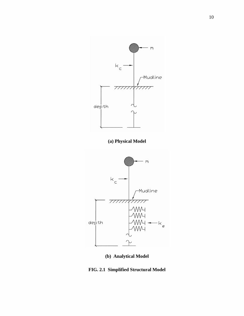
during earthquakes. Fig. 2.1 depicts the basic simplified physical and analytical models

of a structure with lumped mass, m, structural stiffness, kc, and soil properties shown as a

series of equivalent soil springs, ke. Structural and soil properties, along with the intensity

and frequency characteristics of the ground motions, play important roles in the

performance of a structure during earthquakes.

10

(a) Physical Model

(b) Analytical Model

FIG. 2.1 Simplified Structural Model

11

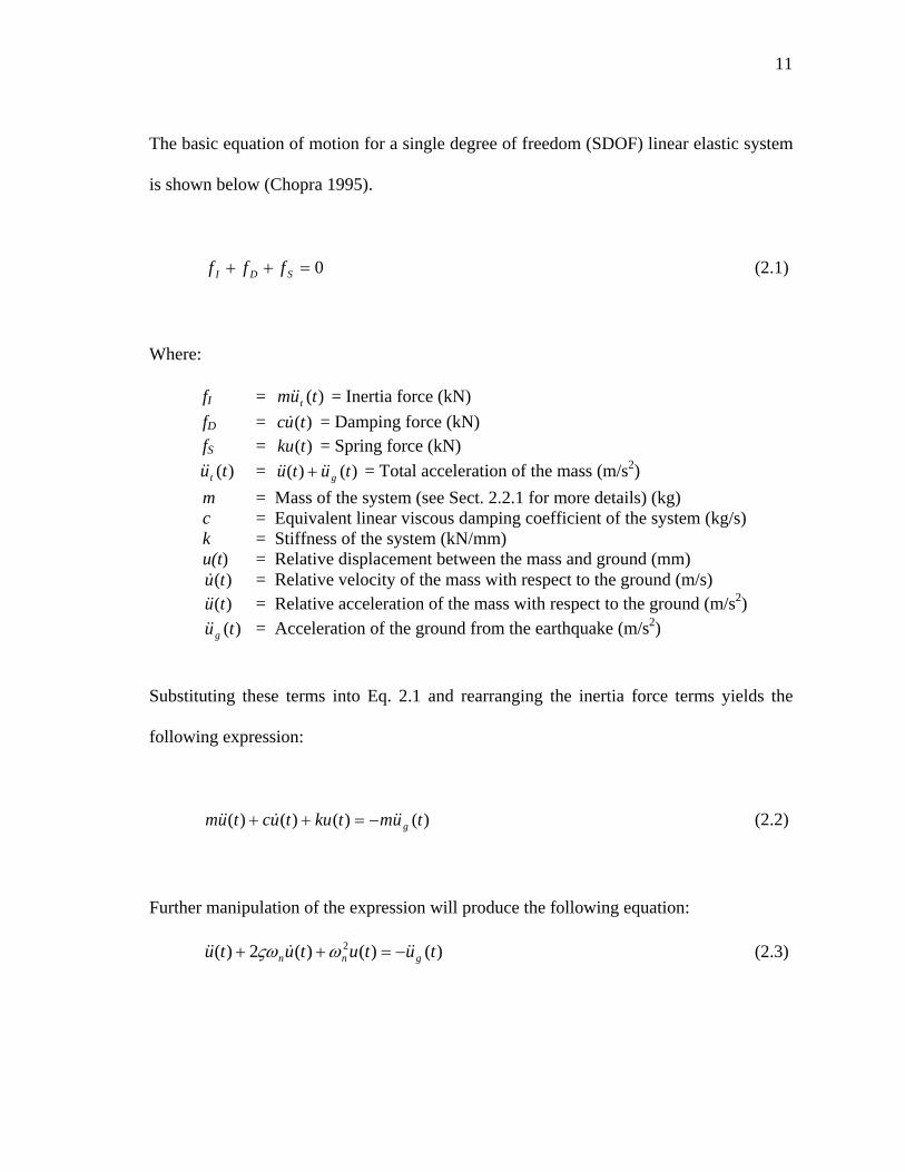
The basic equation of motion for a single degree of freedom (SDOF) linear elastic system

is shown below (Chopra 1995).

0=++ SDI fff (2.1)

Where:

fI = = Inertia force (kN) )(tum t&&

fD = = Damping force (kN) )(tuc &fS = = Spring force (kN) )(tku

= = Total acceleration of the mass (m/s)(tut&& )()( tutu g&&&& + 2) m = Mass of the system (see Sect. 2.2.1 for more details) (kg)

c = Equivalent linear viscous damping coefficient of the system (kg/s) k = Stiffness of the system (kN/mm) u(t) = Relative displacement between the mass and ground (mm)

= Relative velocity of the mass with respect to the ground (m/s) )(tu& = Relative acceleration of the mass with respect to the ground (m/s)(tu&& 2) = Acceleration of the ground from the earthquake (m/s)(tug&&

2)

Substituting these terms into Eq. 2.1 and rearranging the inertia force terms yields the

following expression:

)()()()( tumtkutuctum g&&&&& −=++ (2.2)

Further manipulation of the expression will produce the following equation:

)()()(2)( 2 tutututu gnn &&&&& −=++ ωςω (2.3)

12

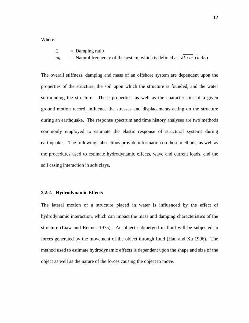
Where:

ζ = Damping ratio ωn = Natural frequency of the system, which is defined as mk / (rad/s)

The overall stiffness, damping and mass of an offshore system are dependent upon the

properties of the structure, the soil upon which the structure is founded, and the water

surrounding the structure. These properties, as well as the characteristics of a given

ground motion record, influence the stresses and displacements acting on the structure

during an earthquake. The response spectrum and time history analyses are two methods

commonly employed to estimate the elastic response of structural systems during

earthquakes. The following subsections provide information on these methods, as well as

the procedures used to estimate hydrodynamic effects, wave and current loads, and the

soil casing interaction in soft clays.

2.2.2. Hydrodynamic Effects

The lateral motion of a structure placed in water is influenced by the effect of

hydrodynamic interaction, which can impact the mass and damping characteristics of the

structure (Liaw and Reimer 1975). An object submerged in fluid will be subjected to

forces generated by the movement of the object through fluid (Han and Xu 1996). The

method used to estimate hydrodynamic effects is dependent upon the shape and size of the

object as well as the nature of the forces causing the object to move.

13

The added mass method is a simplified approach to approximate the effects of

hydrodynamic interaction. Because it is assumed that the motion of an object or structure

in water corresponds to a steady periodic motion, the acceleration of this structure will

also be periodic. In addition, because this method assumes that the hydrodynamic

pressure is in phase with respect to the periodic acceleration of the structure, the impact

on the damping characteristics is negligible (Liaw and Reimer 1975). In this approach,

the force is the product of the mass of the fluid displaced by the movement of the object

(“added mass”) and the acceleration of the object. As stated in API-RP2A, the mass used

for the dynamic analysis of an offshore structure should include the mass of the structure,

fluids contained within the structure, appurtenances, and the added mass (API 2000a,b).

In other words, mass is added to the mass of the structure and its contents for dynamic

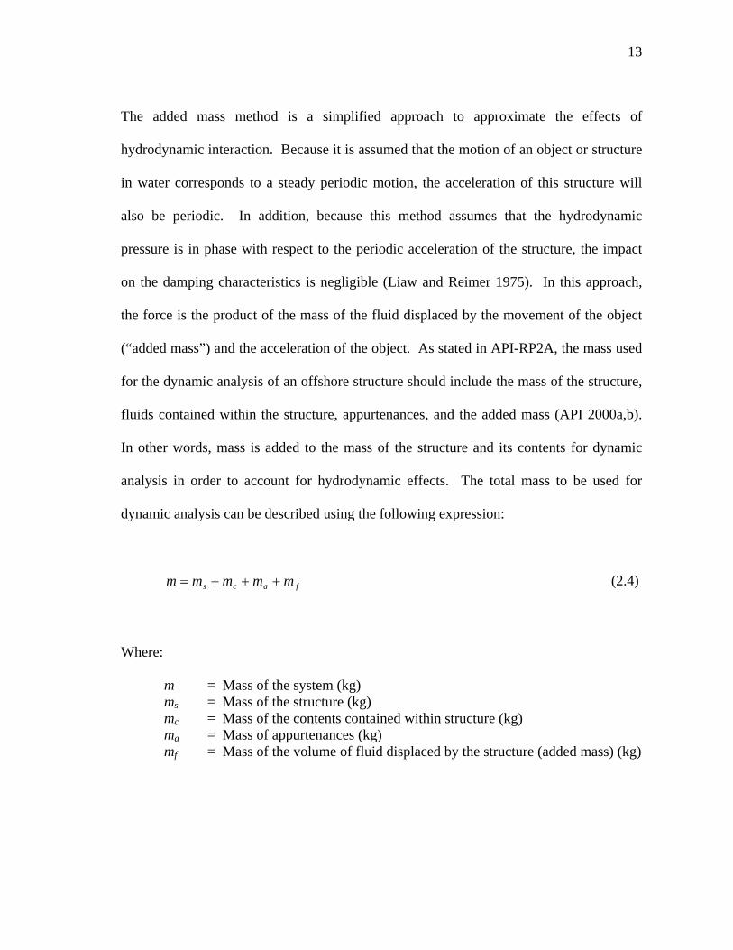
analysis in order to account for hydrodynamic effects. The total mass to be used for

dynamic analysis can be described using the following expression:

facs mmmmm +++= (2.4)

Where:

m = Mass of the system (kg) ms = Mass of the structure (kg) mc = Mass of the contents contained within structure (kg) ma = Mass of appurtenances (kg) mf = Mass of the volume of fluid displaced by the structure (added mass) (kg)

14

2.2.3. Forces Due to Waves and Currents

Another important environmental factor in the structural design of offshore structures is

the force generated by waves and currents. API-RP17A indicates that loads generated by

currents affect the structural design of subsea systems (API 1996). The direction, strength

and other characteristics of these forces are influenced by a number of different factors.

The height, shape, and velocity of surface waves are influenced primarily by wind

characteristics (API 2000 a,b). Three common types of currents are storm-generated

currents, tidal currents, and circulational currents. Because of the various ways these

forces are created, predicting the direction, wave height, and velocity is complicated. A

thorough evaluation of the installation site is necessary in order to gain the necessary

information required to estimate wave and current characteristics for structural design of

an offshore structure.

There are several methods available for estimating the wave and current profiles used to

determine the forces acting on an offshore structure. The method used to estimate water

particle velocity and acceleration due to waves and currents includes the contributions of

the observed conditions at the installation site and the complexity of the proposed

offshore structure. Once these quantities are known, the expression known as Morison’s

equation (Dean and Borgman 1986) can be used to obtain the forces experienced by

individual elements in the structure. This expression, seen in Eq. 2.5, is typically used to

quantify the wave or current forces acting on slender cylindrical elements.

15

SvDC

vvDCtf mD ∆⎥⎦

⎤⎢⎣

⎡+= &

42)(

2ρπρ (2.5)

Where:

CD = Drag coefficient Cm = Inertia coefficient v = Velocity of the water (m/s) = Acceleration of the water (m/sv& 2) ∆S = Length of the element (m) ρ = Density of water (kN/m3)

Both the drag coefficient and the inertia coefficient are dependent upon the shape of the

structural element.

It should be noted that the subsea systems included in this study are located at deepwater

sites, where wave interaction is negligible. On the other hand, mudline currents at these

depths can be significant. Although this is the case, the mudline currents are neglected in

this work.

2.2.4. Soil-Casing Interaction for Soft Clays

Structural response to lateral loading is heavily dependent upon the soil conditions, the

foundation type, and the interaction between the structure and soil. Modeling soil-

structure interaction for the casings (herein referred to as piles) is critical in determining

the seismic response of a subsea structure. The characteristics of the soil-pile behavior

16

are dependent upon the soil and structural geometry, along with the elastic behavior of the

pile.

The relationship between the pile and surrounding soil can be modeled as a complex

beam-column placed on an inelastic foundation. The soil is represented as a series of

uncoupled springs which act along the pile to resist lateral forces applied to the structure

(refer to Fig. 2.1). The governing equation which describes the lateral response of the pile

to static loads (Cox and McCann 1986).

⎟⎠⎞

⎜⎝⎛+=++⎟

⎠⎞

⎜⎝⎛ ′

−dxT

dxdpyE

dxQyd

dxxfR

dxd

dxydEI S 02

20

4

4 )()( (2.6)

Where:

E = Modulus of elasticity of the pile (kPa) I = Moment of inertia of the pile (mm4) y = Lateral displacement of the pile at some point x along the length of the pile (mm) x = Coordinate along the pile axis (mm) R = Load-displacement rate for a rotational restraint (kN/mm) Q = Axial load acting on the pile (kN) T = Applied moment (kN-m) Es = Load displacement rate for the soil (kPa) p0 = Applied distributed lateral load along the pile (shown as p in Fig. 2.2) (kN/mm)

) = (0 xf ′dxdy = slope

17

The solution to this equation can be obtained through the use of difference equation

techniques (Reese and Wang 1986), which includes the use of the expression shown in

Eq. 2.7, with each term described in Eqs. 2.8 through 2.13.

iiiiiiiiiii fyeydycybya =++++ ++−− 2112 (2.7)

11 25.0 −− −= iii hRFa (2.8)

( ) 12

12 −− ++−= iiii QhFFb (2.9)

( ) Siiiiiii EhQhRRhFFFc 41

21111 225.04 +−++++= −+−+− (2.10)

( ) 12

12 ++ ++−= iiii QhFFd (2.11)

11 25.0 ++ −= iii hRFe (2.12)

)(5.0 1123

−+ −+= iiii TThPhf (2.13)

Where:

h = Increment length along the pile (m) Fi = EI (kN/mm) Pi = Applied concentrated load, h*p (kN)

Gaussian elimination can be used to obtain the solution of the expression in Eq. 2.7 with

the appropriate boundary conditions and a sufficient number of increments along the

length of the pile since the soil stiffness varies with displacement, the equations are

nonlinear and an iterative solution technique are used (Reese and Wang 1986). The

beam-column solution is used to calculate the displacement, slope, moment, shear, and

lateral loading at each specified increment along the length of the pile (Cox and McCann

18

1986). These quantities are then used to determine the maximum axial, bending and

combined stresses in the pile, which are in turn compared to the allowable stresses in a

design procedure. It should be mentioned that in this idealization, the mass of the pile and

soil are ignored, i.e. the pile response is treated as quasi-static behavior. This assumption

is based on the fact that the soil pile system has very high natural frequencies relative to

the primary exciting frequencies of the earthquakes. Thus the soil-pile system can be

approximated by a simple non-linear spring system.

The soil resistance characteristics are described through the use of p-y curves, which

represent the soil resistance to pile displacement at a given location along the length of the

pile. A few different approaches can be used to construct p-y curves. Typically these

curves are site specific and are constructed using stress-strain data obtained from soil

samples taken from the location under consideration. In addition, p-y curve construction

is dependent upon the soil type (API 2000 a,b). Typically, the soils found in the GOM

consist of soft clays; therefore, the corresponding p-y curves for this soil type should be

used. API-RP2A refers designers to “Correlations for Design of Laterally Loaded Piles in

Soft Clay” (Matlock 1970) to obtain further information on the construction of p-y curves

for soft clay. This publication states that the shape of the p-y curve is dependent upon the

type of lateral load applied to the structure, as well as the pile stiffness, geometry and soil

characteristics. For the research presented in Matlock’s paper, p-y curves were developed

using a combination of laboratory experiments, field testing, and numerical analysis. The

objective was to confirm that a reasonable model of the soil-pile interaction could be

19

developed that was consistent with experiments and analysis. Based on the results of the

study, Matlock concluded that soil resistance – deflection characteristics are nonlinear and

inelastic, and that within a practical range, the characteristics of the p-y curve were

unaffected by the type of pile head restraint.

2.2.5. Spectral Analysis Method

One approach to approximate the response of a structure during an earthquake event is the

spectral analysis, or response spectrum, method. An elastic response spectrum shows the

peak elastic response of a SDOF oscillator with constant damping as a function of natural

period (or frequency) when subjected to a specified ground motion (Chopra 1995). A

response spectrum plot typically consists of peak deformation, velocity, acceleration, or a

combination of these values with respect to the natural period of the structure. The shape

of a response spectrum of an actual earthquake record is often somewhat erratic.

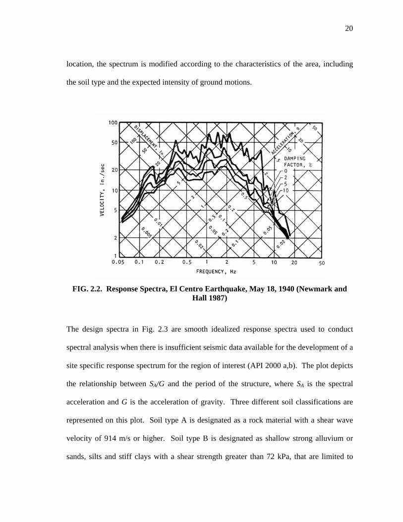
However, when the spectra are plotted on a logarithmic scale, as shown in Fig. 2.2, the

general shape of the plot begins to resemble a trapezoid (Newmark and Hall 1987).

Use of the spectral analysis method for structural design is most appropriate for cases

when the structure is expected to behave elastically (Chopra 1995). In general, available

ground motion records are insufficient for the construction of a site specific design

spectra. For this reason, the analysis is performed using a generalized design spectrum.

The design spectrum is a smoothed curve based on statistical analysis of a variety of

different ground motions. In order to perform the design of a structure at a specific

20

location, the spectrum is modified according to the characteristics of the area, including

the soil type and the expected intensity of ground motions.

FIG. 2.2. Response Spectra, El Centro Earthquake, May 18, 1940 (Newmark and

Hall 1987)

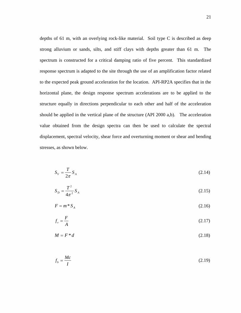
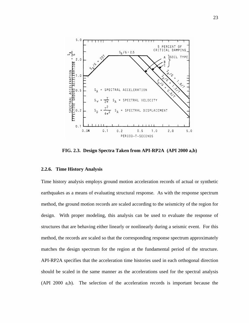
The design spectra in Fig. 2.3 are smooth idealized response spectra used to conduct

spectral analysis when there is insufficient seismic data available for the development of a

site specific response spectrum for the region of interest (API 2000 a,b). The plot depicts

the relationship between SA/G and the period of the structure, where SA is the spectral

acceleration and G is the acceleration of gravity. Three different soil classifications are

represented on this plot. Soil type A is designated as a rock material with a shear wave

velocity of 914 m/s or higher. Soil type B is designated as shallow strong alluvium or

sands, silts and stiff clays with a shear strength greater than 72 kPa, that are limited to

21

depths of 61 m, with an overlying rock-like material. Soil type C is described as deep

strong alluvium or sands, silts, and stiff clays with depths greater than 61 m. The

spectrum is constructed for a critical damping ratio of five percent. This standardized

response spectrum is adapted to the site through the use of an amplification factor related

to the expected peak ground acceleration for the location. API-RP2A specifies that in the

horizontal plane, the design response spectrum accelerations are to be applied to the

structure equally in directions perpendicular to each other and half of the acceleration

should be applied in the vertical plane of the structure (API 2000 a,b). The acceleration

value obtained from the design spectra can then be used to calculate the spectral

displacement, spectral velocity, shear force and overturning moment or shear and bending

stresses, as shown below.

AV STSπ2

= (2.14)

AD STS 2

2

4π= (2.15)

ASmF *= (2.16)

AFfv = (2.17)

dFM *= (2.18)

IMcfb = (2.19)

22

Where:

SV = Spectral Velocity (m/s) SD = Spectral Displacement (m) T = Fundamental period (s) F = Shear force applied to structural element (kN) fv = Shear stress acting on structural element (kPa) A = Area of structural element (m2) M = Overturning moment acting on structural element (kN-m) d = Length of the moment arm (m) fb = Bending stress acting on structural element (kPa) I = Moment of inertia of structural element (mm4) c = Distance from extreme edge to the centroid of structural element (mm)

Finally, the stress and displacement values obtained are compared to the allowable

stresses and displacements to determine the adequacy of the element for the seismic

demand.

23

FIG. 2.3. Design Spectra Taken from API-RP2A (API 2000 a,b)

2.2.6. Time History Analysis

Time history analysis employs ground motion acceleration records of actual or synthetic

earthquakes as a means of evaluating structural response. As with the response spectrum

method, the ground motion records are scaled according to the seismicity of the region for

design. With proper modeling, this analysis can be used to evaluate the response of

structures that are behaving either linearly or nonlinearly during a seismic event. For this

method, the records are scaled so that the corresponding response spectrum approximately

matches the design spectrum for the region at the fundamental period of the structure.

API-RP2A specifies that the acceleration time histories used in each orthogonal direction

should be scaled in the same manner as the accelerations used for the spectral analysis

(API 2000 a,b). The selection of the acceleration records is important because the

24

response of the structure is sensitive to the frequency content and magnitude of the

accelerations (Nair and Kallaby 1986). Therefore, records should be used that contain

characteristics representative of the conditions at the proposed installation site.

2.3. PREVIOUS SEISMIC RESEARCH OF OFFSHORE SYSTEMS

The literature contains many studies on various aspects of earthquake analysis for

offshore structures. The following subsections present research findings related to this

study, including studies of the seismic behavior of fixed offshore platforms, piles, and

subsea pipelines. Also included in this section is a summary of research related to the

characteristics of ground motions at offshore locations. Although the topics covered by

the studies cited in the following subsections are somewhat varied, each provides useful

guidelines and insight for the investigation of the deepwater subsea systems considered in

this study.

2.3.1. Offshore Ground Motions

Smith (1997) studied the differences between onshore and offshore ground motions. A

comparison was made between measurements taken during the September 1981 Santa

Barbara Island, California earthquake at nearby onshore and offshore locations. This

event was selected because of the comparable epicentral distances to the land based

instruments and the Seafloor Earthquake Measurement System (SEMS) instruments. The

onshore site, SBVictor, was located 98 km from the epicenter of the earthquake and the

25

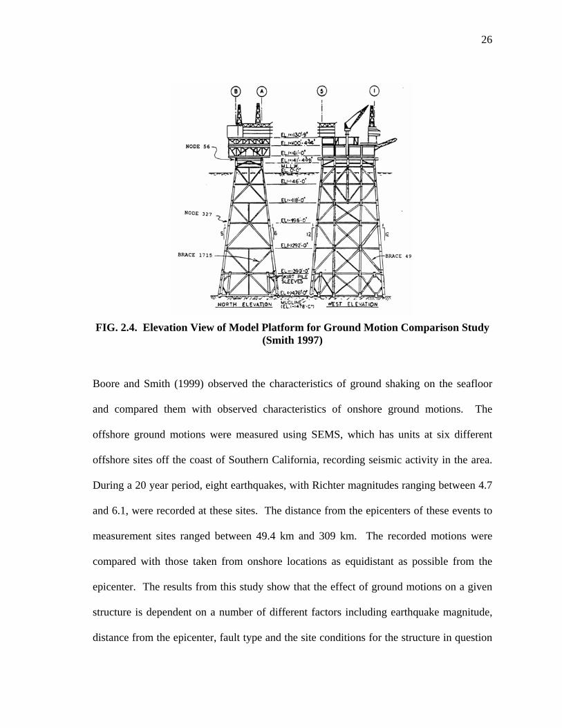
offshore site, SBHenry, was approximately 85 km. The platform model used for this

study was approximately 185 m in height and located in 145 m of water (see Fig 2.4).

The jacket was supported by a group of four piles at each of the four corners. A seismic

response analysis was performed on the platform using the Santa Barbara Island records

scaled to match the API spectrum with an acceleration of 0.25g. In addition, the soil

stiffness was varied to simulate stiff clay, soft clay, and dense sand conditions.

Comparisons between the different soil types show that the periods obtained for the

models founded in soft clays were between 101 and 162 percent of the values obtained

from the models located in either stiff clay or dense sand. The vertical deflections

observed for the offshore earthquake record were between 24.8 and 61.1 percent of the

values observed for the onshore records. The total vertical accelerations generated by the

offshore records were between 25.8 and 46.2 percent of those observed in the platform

models subjected to the onshore accelerations. A comparison between the results from

the onshore records and the results from the offshore records show that the differences in

the vertical component are due to the presence of the water layer over the offshore site. In

conclusion, this study demonstrates that the vertical component of the measurement

recorded at the offshore location was significantly smaller than that of the onshore record.

26

FIG. 2.4. Elevation View of Model Platform for Ground Motion Comparison Study

(Smith 1997)

Boore and Smith (1999) observed the characteristics of ground shaking on the seafloor

and compared them with observed characteristics of onshore ground motions. The

offshore ground motions were measured using SEMS, which has units at six different

offshore sites off the coast of Southern California, recording seismic activity in the area.

During a 20 year period, eight earthquakes, with Richter magnitudes ranging between 4.7

and 6.1, were recorded at these sites. The distance from the epicenters of these events to

measurement sites ranged between 49.4 km and 309 km. The recorded motions were

compared with those taken from onshore locations as equidistant as possible from the

epicenter. The results from this study show that the effect of ground motions on a given

structure is dependent on a number of different factors including earthquake magnitude,

distance from the epicenter, fault type and the site conditions for the structure in question

27

(Boore and Smith 1999). In general, ground motions at an offshore site were found to be

the same as ground motions at an onshore site. In other words, the effects of a given

earthquake are considered to be the same for onshore and offshore sites. However, results

from this study show that the sediment layer and the water volume over the site dampen

the vertical component of the ground motion. As a result, the V/H ratios (vertical to

horizontal component of motion) for offshore locations are smaller than those with

comparable characteristics at onshore locations. In addition, the amount of damping is

proportional to the period of the ground motions, such that the difference between the

vertical component of the onshore motions and the offshore motions increased as the

periods became shorter and decreased as the periods became longer. Finally, the results

also showed that the horizontal component of the motion did not vary much between

offshore and onshore sites having comparable characteristics.

2.3.2. Seismic Analysis of Fixed Platforms

Boote and Mascia (1994) studied the application of the response spectra method and the

time history analysis method for evaluating the seismic behavior of a fixed offshore

platform. Both methods were designed to represent an envelope of seismic excitation of

the platform consistent with the seismicity of the region. Typically, several ground

motion records from different earthquakes should be used for the analysis in order to

formulate a comprehensive picture of the effects of different input motions on variations

in the response of the platform (API 2000 a,b).

28

The fixed platform analytical model used in the above study was a four-leg jacket with

bracing in the vertical and horizontal planes of the jacket. The jacket was modeled with

and without foundation piles. To analyze the model without foundation piles, the jacket

was assumed to be fixed at the ground level. In the jacket model with foundation piles,

the piles were modeled as a series of horizontal springs with varying stiffness values,

which accounted for the soil-pile interaction with linear elastic behavior. An added mass,

taken as a percentage of the water volume displaced by the submerged portion of the

structure, was used to account for the water-structure interaction. For the hypothetical

location of the platform, the soil type was assumed to be “rock”, represented by curve “A”

in the API design spectrum, with Zone 2 seismicity, corresponding to accelerations of

0.1g. For both analysis methods, ground accelerations recorded from the 1952 Taft, CA

and 1940 El Centro, CA earthquakes were applied to the model and scaled down for Zone

2 seismicity. For both events, earthquake durations of 20 seconds were selected for the

study, as specified in the Eurocode. These records were chosen because they are both

Class II earthquakes typical for compact ground with irregular movements and extended

duration, although the accelerations from the El Centro record are approximately 19

percent higher than that of the Taft record (Boote and Mascia 1994). In addition, the

damping ratios were varied from 0.005 to 0.05 to observe the influence of damping on the

stresses and deflections estimated by the model.

The results from the analyses were presented in the form of structural displacements and

forces produced by the ground motions. The results from the spectral analyses show that

29

the spectra from the scaled Taft and El Centro earthquakes produced higher stresses and

deflections than those produced by the design spectrum. The time history analyses, which

used Taft and El Centro measured ground accelerations, yielded force and deflection

values smaller than those produced by the spectral analyses. Based on the results from

this study, the authors concluded that the use of the spectral analysis method for

evaluating seismic response of offshore structures is a conservative approach.

Boote et al. (1998) continued to study response spectra and time history analysis methods

with varying design spectra and time history accelerations. The model used for the study

was based on a platform located in the Adriatic Sea. The jacket consisted of eight legs,

braced horizontally and vertically, supporting the main deck (46 m by 21 m) and the cellar

deck (36 m by 12 m). The structure was approximately 46 m high and was located in 30

m of water. The foundation piles were 70 m deep and the soil consisted of five distinct

layers, which were assumed to behave elastically for the analysis. Analyses of the

platform were conducted using five different numerical models with varying parameters

for the soil-structure interaction, added mass, presence of conductors, and foundation. The

first model, Model A, was constructed by schematizing all of the structural components of

the jacket and platform. Model B included consideration of added mass in the portion of

the jacket under water. Models C and D included the conductors, which run vertically

from the deck down through the jacket to the seafloor. Model D included the added mass

of the submerged portion of the structure and Model C excluded consideration for

hydrodynamic effects. Fig. 2.5 illustrates the numerical model used for Model F, which

30

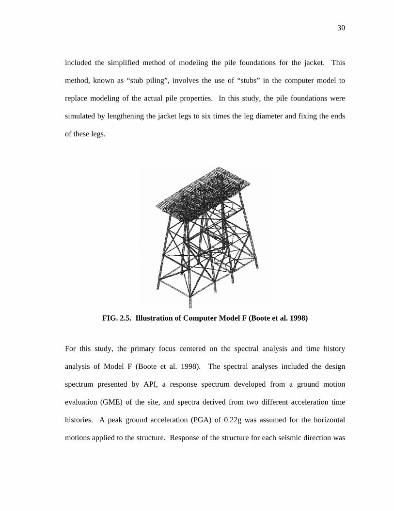
included the simplified method of modeling the pile foundations for the jacket. This

method, known as “stub piling”, involves the use of “stubs” in the computer model to

replace modeling of the actual pile properties. In this study, the pile foundations were

simulated by lengthening the jacket legs to six times the leg diameter and fixing the ends

of these legs.

FIG. 2.5. Illustration of Computer Model F (Boote et al. 1998)

For this study, the primary focus centered on the spectral analysis and time history

analysis of Model F (Boote et al. 1998). The spectral analyses included the design

spectrum presented by API, a response spectrum developed from a ground motion

evaluation (GME) of the site, and spectra derived from two different acceleration time

histories. A peak ground acceleration (PGA) of 0.22g was assumed for the horizontal

motions applied to the structure. Response of the structure for each seismic direction was

31

calculated using both the Square Root of the Sum of the Squares (SRSS) combination

method and the Complete Quadratic Combination (CQC) method for each response

spectra studied. The time history analyses were conducted using two different

acceleration records, labeled TH1 and TH2. These records were also used to construct the

response spectra used for the spectral analysis of the platform. As with the response

spectra analyses, both records were scaled to a PGA value of 0.22g.

For each of the different analyses, spectra, and combination methods, a comparison was

made of the stresses obtained at the seabed level for each of the platform legs (Boote et al.

1998). The results indicate that the API spectrum yields more severe results than the

GME spectrum. In addition, the CQC method yields higher stress values than that of the

SRSS combination method for all of the spectral analysis results. Finally, the differences

between the results obtained by spectral analysis and those obtained from time history

analysis are less than six percent, demonstrating the suitability of the spectral analysis

method for linear analysis.

2.3.3. Pile Behavior Under Seismic Loading

Michalopoulos et al. (1984) examined the process of designing the foundations of

offshore structures to resist earthquake loads. Because of the differences that exist

between onshore and offshore buildings and site conditions, building codes typically used

for onshore structures are not applicable for the design of offshore structures

(Michalopoulos et al. 1984). The process used for foundation design involves several

32

different steps, which include the development of time history records appropriate to the

seismicity of the site, conducting a soil-pile-structure-water analysis, determining the

static stiffness of the pile, and determining the pile loads from the structure and the soil.

The type of mathematical model used to simulate a structure and foundation subjected to

ground motions heavily influences the analysis results (Michalopoulos et al. 1984). Four

important characteristics considered for the selection of these models were the foundation

type, water depth, required efficiency during the design phase, and the influence of higher

modes on member forces. To demonstrate the importance of proper model selection, the

paper cites the example of a fixed platform, 117 m high, located in a depth of 106 m in the

Mediterranean Sea (Michalopoulos et al. 1984). Each of the four jacket legs was

supported by a group of four 83 m long piles. Modal analyses were conducted on a

lumped mass model and a structural frame model of the platform. The seismic risk for

this model was based on the seismicity of a site near Viking Graben in the North Sea.

According to the probabilistic analysis of the seismic risk of this region, the strength level

earthquake (SLE) was 0.25g, and the ductility level earthquake (DLE) was greater than

0.4g, based on earthquake data recorded in this area between 1970 and 1981.

Because the lumped mass model was only two dimensional, the analysis produced

frequencies for one lateral direction (Michalopoulos et al. 1984). However, frequency

values for both lateral components of motion were obtained for the structural frame

model. A comparison of the results from the two models indicated that the frequency

33

values for the lumped mass model were approximately 37 to 137 percent larger than the

frequencies obtained for either lateral component of the structural frame model.

Rao and O’Neill (1997) studied the response of piles to earthquake loads and evaluated

the effect of variations in the earthquake magnitude. In order to study the response of

seismically loaded piles, a scaled laboratory model was subjected to three different

horizontal accelerations corresponding to California-type earthquakes. The model

consisted of a steel pipe driven into fine sand inside a chamber filled with water. The pipe

dimensions were 25.4 mm outer diameter with a 1.4 mm wall thickness and 405 mm in

length. Tension loads, varying between approximately 45 to 90 percent of the pile static

capacity, were applied at the top of the pile. The magnitude of the motions were 7.0, 7.5,

and 8.0 Richter magnitudes scaled up from ground accelerations recorded for the Upland

1990 and Oceanside 1986 earthquakes events in California, both records were for Richter

magnitude 5.0 events. The accelerograms were obtained from an offshore deep sand site

near Long Beach, California, approximately 75 km from both events.

Results from thirteen of the horizontal shaking tests were reported, displaying the

behavior of the pile under various seismic and static tension loads. For the range of

tension load values used in this experiment, the pile did not experience failure under the

Richter magnitude 7.0 seismic loading (Rao and O’Neill 1997). Pullout of the pile

occurred at 91 percent of the static capacity under the magnitude Richter magnitude 7.5

loading and 78 percent of the static axial tension capacity for the Richter magnitude 8.0

34

loading. In addition, the pile remained stable up to 65, 60, and 45 percent of the static

capacity for the magnitude 7.0, 7.5, and 8.0 seismic events, respectively. Therefore, it

was found that as the magnitude of the seismic event increases, the pile will lose stability

for increasingly smaller tension loads, consistent with expectations.

2.3.4. Subsea Pipelines Under Seismic Loading

Jones (1985) discussed some of the environmental considerations that impact the loading

for deepwater pipelines as part of a feasibility study conducted for Shell Development

Company. The pipe sizes included in this study ranged from 305 mm up to 1067 mm

outside diameter for water depths ranging from 183 m to 914 m. Two of the

environmental factors examined in the study were bottom currents and earthquakes.

Research on deepwater bottom currents consisted of gathering general background

information, including a list of all available measured current velocities for deepwater

locations at the time of the study. In addition, a design current velocity of 0.91 m/s was

recommended for situations where information on the currents is unavailable. Jones

(1985) developed two diagrams (shown in Fig. 2.6) to illustrate the impact of ground

motions on a pipeline with respect to earthquake magnitude and proximity.

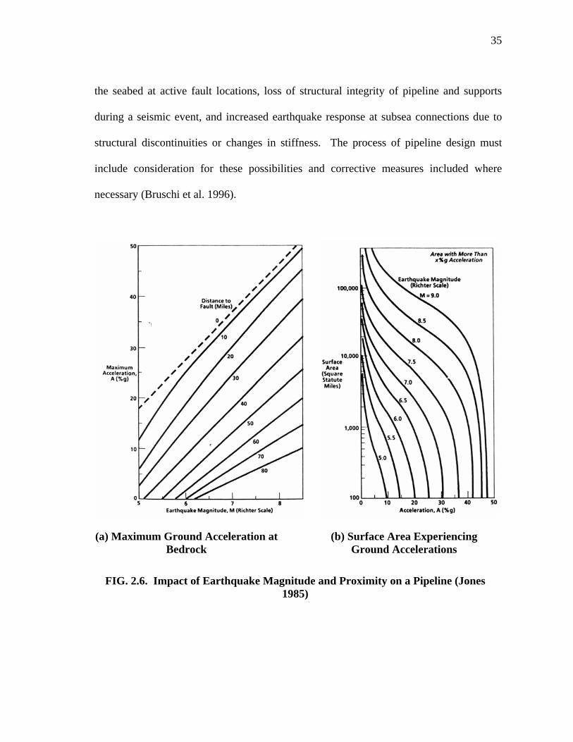
Bruschi et al. (1996) reviewed current procedures for seismic design of offshore pipelines

placed in seismically active areas. Some of the problems encountered as a result of an

earthquake are the loss of soil stability due to seismic excitation, steep discontinuities in

35

the seabed at active fault locations, loss of structural integrity of pipeline and supports

during a seismic event, and increased earthquake response at subsea connections due to

structural discontinuities or changes in stiffness. The process of pipeline design must

include consideration for these possibilities and corrective measures included where

necessary (Bruschi et al. 1996).

(a) Maximum Ground Acceleration at Bedrock

(b) Surface Area Experiencing Ground Accelerations

FIG. 2.6. Impact of Earthquake Magnitude and Proximity on a Pipeline (Jones 1985)

36

The first step in the design process is to evaluate the seismic hazard and soil stability for

the proposed installation site (Bruschi et al. 1996). The next step is to examine the

pipeline integrity. The pipeline deforms with the soil because it acts as one body with

the soil. The response of the pipeline to earthquake loading is affected by the pipe

properties, suspended pipe lengths, characteristics of the seabed, soil-pipeline

interaction, and the axial load applied to the pipeline prior to the seismic event. Of

primary concern in seismic design for pipelines is the stress experienced by the pipeline

at the support locations. If the stresses exceed the allowable limit, then additional

supports must be added to shorten the unsupported span length. Except for instances

where a number of risk factors are present in the pipeline and site conditions, seismic

excitations alone will not cause significant damage (Bruschi et al. 1996).

According to Kershenbaum et al. (1998), the behavior of subsea pipelines under seismic

loading is dependent on the magnitude of the seismic event, seabed characteristics,

geometry and properties of the pipeline prior to the seismic event. Although the pipeline

is straight at the time of installation, snaking, or bending in the pipeline, caused by

thermal and internal pressure on the pipe, will eventually change the shape of the line

over time. The amount of bending increases at points in the line where the ends are

restrained.

The authors present a method of earthquake analysis for unburied pipelines subjected to

fault dislocation, which includes consideration of the initial shape of the pipeline

37

(Kershenbaum et al. 1998). The factors used to quantify the behavior of the seismically

loaded pipeline include the earthquake magnitude, shape of the overall pipeline, soil

properties, and the type of fault over which the pipeline has been placed. For this study,

several different pipeline models with varying fault types and various degrees of bending

were subjected to earthquake loading equivalent to Richter magnitude 6 and 7 seismic

events.

The final results from the analysis of several different models show that increasing the

magnitude of ground motions causes small increases in the stresses measured in the

pipelines. Snaking, or deformation from the original pipeline shape, resulted in an

amplification of the stress equal to 1.65 when the earthquake strength changed from

Richter magnitude 6 to 7 (Kershenbaum et al. 1998). The stress amplification for the

vertical component of reverse-slip fault movement was 1.2 and 1.05 for oblique slip fault

movement. The final conclusion of the study was to recommend that the design of

pipelines include consideration for snaking.

2.3.5. Conclusion

The studies presented by Smith (1997) and Boore and Smith (1999) indicate that the

horizontal component of ground motions observed at offshore locations are similar to

those observed at onshore locations, while the vertical component of the offshore ground

motions are often significantly lower. These results indicate that the current practice of

using onshore ground motions for the design of offshore structures is acceptable. As

38

shown in the studies listed above, the use of spectral analysis and time history analysis

methods are reasonable methods for evaluating the response of offshore structures to

earthquake loadings. The study presented by Jones (1985) provides information on the

type of environmental loads that deepwater pipelines will experience, which are similar

to the loads applied to subsea structures. Finally, the research presented by Bruschi et al.

(1996) and Kershenbaum et al. (1998) indicate that the primary points of concern along

the pipeline section are at the supports and locations where the pipeline connects to

subsea systems. Therefore consideration should be given to the loads that pipelines

incur on these systems during seismic events.

39

3. SEISMIC DESIGN CRITERIA AND SEISMIC ACTIVITY IN THE GULF OF MEXICO

3.1. INTRODUCTION The purpose of this section is to outline the design criteria for earthquake loading on

offshore structures. Section 3.2 presents the criteria and procedures proposed for the

seismic design of subsea structures. Part of the design process involves identifying site

characteristics, including local seismicity and site conditions, in order to evaluate the

seismic risk. A summary of the earthquakes recorded for the GOM region is also

presented.

3.2. SEISMIC DESIGN CRITERIA

Preliminary design procedures for offshore structures outlined by API-RP2A (API 2000

a,b) include the evaluation of seismicity at and near the proposed installation site. The

evaluation should encompass an investigation of local site conditions, as well as the

surrounding area, in order to make a thorough assessment of the risk to the proposed

structure. The purpose of studying the surrounding area is to determine the location of

potential sources of seismic activity, such as faults, and to gauge the source-to-site

transmission and attenuation properties (API 2000 a,b). The type of faulting and local

soil conditions play an important role in the ground motions transmitted to the structure,

as well as the response of the structure to these motions. Finally, the accelerations or

measured ground motions used for structural design are based upon the seismic

40

intensity, potential duration, frequency content of strong ground motions, and recurrence

interval of previously recorded events for the location.

Offshore structures are designed for two types of seismic events: a strength level

earthquake and a ductility level earthquake. The strength level earthquake is the

strongest event expected to occur at the site within the span of operation for the offshore

structure (API 2000 a,b). The purpose of using the strength level event is to design the

structure so that it will respond to these motions primarily in the elastic region. The

ductility level earthquake is a rare seismic event with a return period of a thousand years

or more. Since this event can be rather large, structures must be designed to withstand

the earthquake without collapsing, although nonlinear response and significant damage

may occur.

The seismicity of the installation site governs the method of analysis used to evaluate the

performance of subsea systems. If the expected earthquake strength is very small, then

the earthquake effects can be neglected in the design process. If the horizontal

accelerations are small but greater than 0.05g, then the structure should be analyzed by

the spectral analysis method for earthquake force demands (API 2000 a,b). Although

the use of the time history analysis method is applicable for these accelerations, this

method can also be used for situations where the strength of the ground motions causes

the structure to behave nonlinearly.

41

Because predicting the occurrence of earthquakes is highly uncertain, offshore systems

can be expected to be operating if a seismic event does in fact occur (API 2000 a,b).

Therefore, the loads under consideration for a seismic event will include operating loads,

as well as dead loads. For subsea production systems, the mass used for the analysis

should include the mass of the structure, attached equipment, fluids contained within the

equipment, and the added mass, typically taken as a fraction of the mass of the volume

of water displaced by the structure. The equivalent linear viscous damping ratio to be

used for an elastic analysis of offshore structures is five percent (API 2000 a,b).

As specified by API-RP2A, the seismicity of an area under scrutiny can be rated

according to relative zone factors (see Fig. 3.1). The effective horizontal ground

acceleration is the product of the zone factor and five percent of the gravitational

acceleration (Z*0.05g). For instance, the strength level design for structures located

within areas rated as Zone 2 will have a predicted peak ground acceleration of 0.10g.

However, the GOM is currently zoned as aseismic and has a relative seismic zone factor

of 0, which means that the effective horizontal ground accelerations for the strength

level earthquake can be neglected since they are less than 0.05g (API 2000 a,b). This

assumption is discussed in the next section.

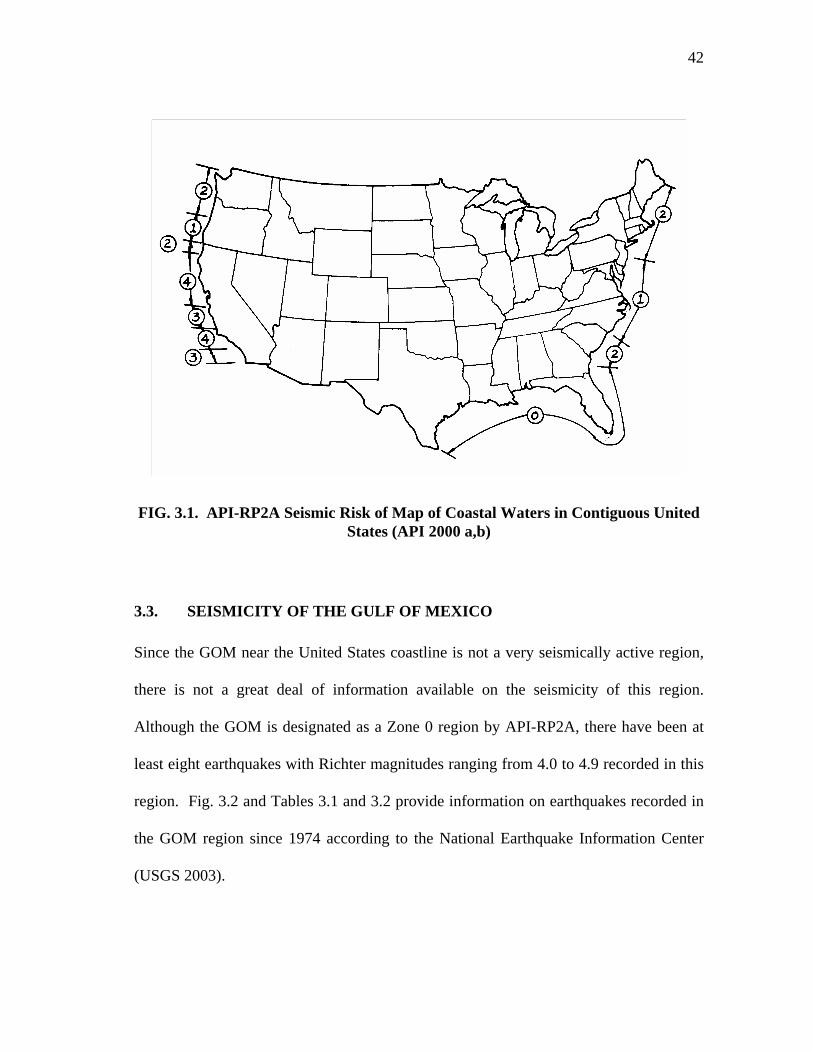
42

FIG. 3.1. API-RP2A Seismic Risk of Map of Coastal Waters in Contiguous United States (API 2000 a,b)

3.3. SEISMICITY OF THE GULF OF MEXICO

Since the GOM near the United States coastline is not a very seismically active region,

there is not a great deal of information available on the seismicity of this region.

Although the GOM is designated as a Zone 0 region by API-RP2A, there have been at

least eight earthquakes with Richter magnitudes ranging from 4.0 to 4.9 recorded in this

region. Fig. 3.2 and Tables 3.1 and 3.2 provide information on earthquakes recorded in

the GOM region since 1974 according to the National Earthquake Information Center

(USGS 2003).

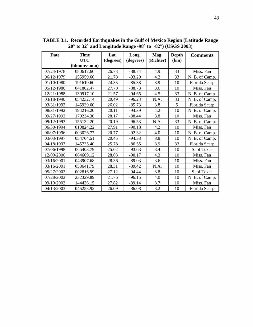
43

TABLE 3.1. Recorded Earthquakes in the Gulf of Mexico Region (Latitude Range 20° to 32° and Longitude Range -98° to -82°) (USGS 2003)

Date Time UTC

(hhmmss.mm)

Lat. (degrees)

Long. (degrees)

Mag. (Richter)

Depth (km)

Comments

07/24/1978 080617.60 26.73 -88.74 4.9 33 Miss. Fan 06/12/1979 155959.60 21.78 -93.20 4.2 33 N. B. of Camp. 01/10/1980 191619.60 24.35 -85.38 3.9 10 Florida Scarp 05/12/1986 041802.47 27.70 -88.73 3.6 10 Miss. Fan 12/21/1988 130917.10 21.57 -94.65 4.5 33 N. B. of Camp. 03/18/1990 054232.14 20.49 -96.23 N.A. 33 N. B. of Camp. 03/31/1992 145939.60 26.02 -85.73 3.8 5 Florida Scarp 08/31/1992 194216.20 20.11 -94.39 4.2 10 N. B. of Camp. 09/27/1992 170234.30 28.17 -88.44 3.8 10 Miss. Fan 09/12/1993 155132.20 20.19 -96.53 N.A. 33 N. B. of Camp. 06/30/1994 010824.22 27.91 -90.18 4.2 10 Miss. Fan 06/07/1996 003026.77 20.77 -92.32 4.0 10 N. B. of Camp. 03/03/1997 054704.51 20.45 -94.33 3.8 10 N. B. of Camp. 04/18/1997 145735.40 25.78 -86.55 3.9 33 Florida Scarp 07/06/1998 065403.79 25.02 -93.63 3.4 10 S. of Texas 12/09/2000 064609.12 28.03 -90.17 4.3 10 Miss. Fan 03/16/2001 043907.68 28.36 -89.03 3.6 10 Miss. Fan 03/16/2001 053641.79 28.31 -89.42 N.A. 10 Miss. Fan 05/27/2002 002816.99 27.12 -94.44 3.8 10 S. of Texas 07/28/2002 232329.89 21.76 -96.15 4.0 10 N. B. of Camp. 09/19/2002 144436.15 27.82 -89.14 3.7 10 Miss. Fan 04/13/2003 045253.92 26.09 -86.08 3.2 10 Florida Scarp

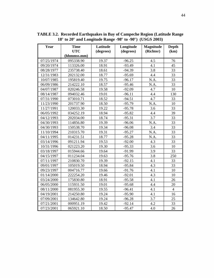
44

TABLE 3.2. Recorded Earthquakes in Bay of Campeche Region (Latitude Range 18° to 20° and Longitude Range -98° to -90°) (USGS 2003)

Year Time UTC

(hhmmss.mm)

Latitude (degrees)

Longitude (degrees)

Magnitude (Richter)

Depth (km)

07/25/1974 095338.90 19.37 -96.25 4.5 76 09/20/1974 113326.00 18.91 -93.49 4.1 45 08/28/1977 235738.40 18.61 -94.39 3.8 33 12/31/1983 202132.00 18.77 -95.69 4.4 33 10/07/1985 195819.40 19.75 -96.17 N.A. 33 06/09/1986 214222.10 18.57 -95.46 N.A. 33 04/07/1987 020246.58 19.58 -92.09 4.7 10 08/14/1987 094032.46 19.01 -96.11 4.4 130 07/31/1990 073010.71 18.52 -94.51 4.7 33 11/23/1990 201737.90 18.50 -95.79 N.A. 10 11/27/1991 120033.30 19.22 -95.78 3.6 33 06/05/1992 034252.19 18.94 -95.82 4.4 39 04/12/1993 202034.00 18.74 -95.31 3.7 33 04/30/1993 114856.80 19.39 -96.06 N.A. 33 04/30/1993 150538.70 19.34 -96.08 3.4 33 11/10/1994 210315.70 19.31 -95.27 N.A. 33 04/11/1995 014231.51 18.77 -95.28 N.A. 33 03/14/1996 091211.94 19.53 -92.00 4.3 33 10/31/1996 021223.20 19.30 -95.33 3.6 10 03/18/1997 015944.66 19.64 -91.99 3.9 33 04/15/1997 011234.04 19.63 -95.76 3.8 250 07/11/1997 210830.70 19.39 -92.15 4.1 33 09/01/1997 105019.50 18.94 -95.84 4.3 33 09/23/1997 004716.77 19.66 -91.76 4.1 10 01/14/2000 222254.20 19.46 -92.01 4.3 10 03/24/2000 175830.80 18.91 -95.58 4.1 26 06/05/2000 115931.50 19.01 -95.68 4.4 20 08/11/2000 081955.30 19.55 -96.41 4.1 4 04/19/2001 214250.80 19.24 -95.90 4.1 16 07/09/2001 134642.80 19.24 -96.28 3.7 25 07/21/2001 000951.19 19.42 -92.14 4.2 33 07/23/2001 065921.10 18.50 -95.47 4.0 26

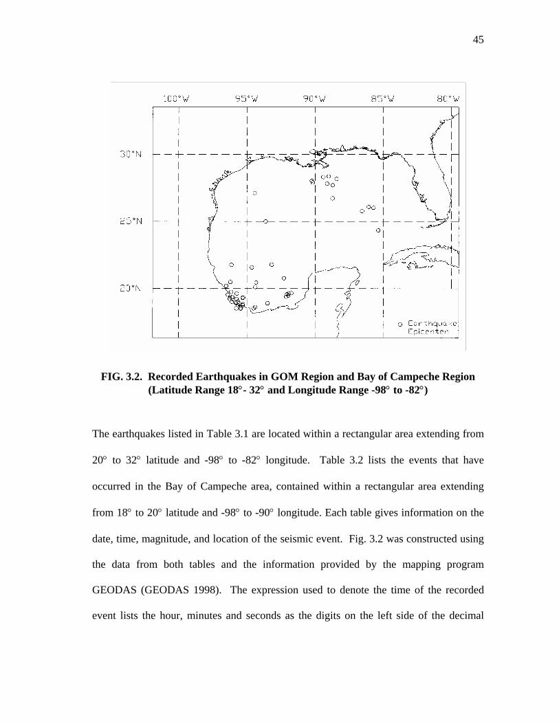
45

FIG. 3.2. Recorded Earthquakes in GOM Region and Bay of Campeche Region (Latitude Range 18°- 32° and Longitude Range -98° to -82°)

The earthquakes listed in Table 3.1 are located within a rectangular area extending from

20° to 32° latitude and -98° to -82° longitude. Table 3.2 lists the events that have

occurred in the Bay of Campeche area, contained within a rectangular area extending

from 18° to 20° latitude and -98° to -90° longitude. Each table gives information on the

date, time, magnitude, and location of the seismic event. Fig. 3.2 was constructed using

the data from both tables and the information provided by the mapping program

GEODAS (GEODAS 1998). The expression used to denote the time of the recorded

event lists the hour, minutes and seconds as the digits on the left side of the decimal

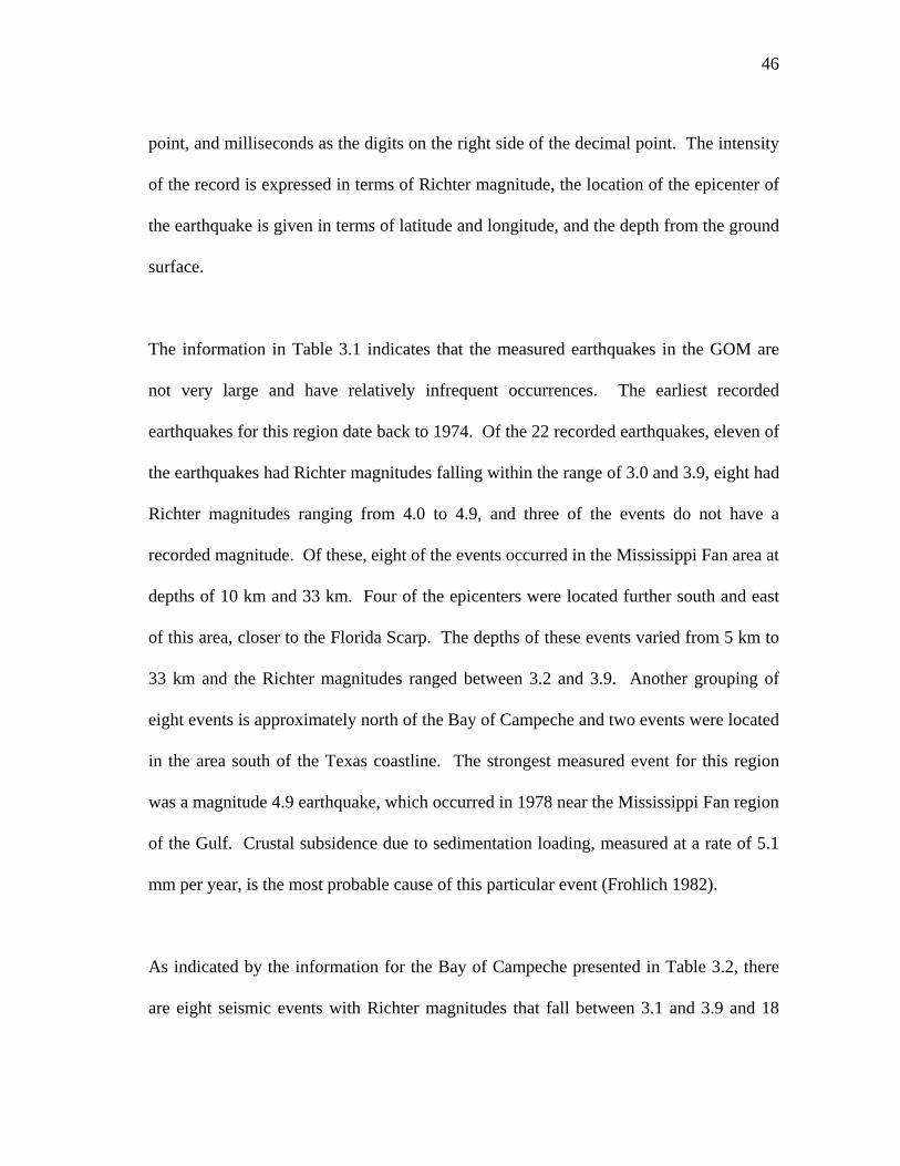
46

point, and milliseconds as the digits on the right side of the decimal point. The intensity

of the record is expressed in terms of Richter magnitude, the location of the epicenter of

the earthquake is given in terms of latitude and longitude, and the depth from the ground

surface.

The information in Table 3.1 indicates that the measured earthquakes in the GOM are

not very large and have relatively infrequent occurrences. The earliest recorded

earthquakes for this region date back to 1974. Of the 22 recorded earthquakes, eleven of

the earthquakes had Richter magnitudes falling within the range of 3.0 and 3.9, eight had

Richter magnitudes ranging from 4.0 to 4.9, and three of the events do not have a

recorded magnitude. Of these, eight of the events occurred in the Mississippi Fan area at

depths of 10 km and 33 km. Four of the epicenters were located further south and east

of this area, closer to the Florida Scarp. The depths of these events varied from 5 km to

33 km and the Richter magnitudes ranged between 3.2 and 3.9. Another grouping of

eight events is approximately north of the Bay of Campeche and two events were located

in the area south of the Texas coastline. The strongest measured event for this region

was a magnitude 4.9 earthquake, which occurred in 1978 near the Mississippi Fan region

of the Gulf. Crustal subsidence due to sedimentation loading, measured at a rate of 5.1

mm per year, is the most probable cause of this particular event (Frohlich 1982).

As indicated by the information for the Bay of Campeche presented in Table 3.2, there

are eight seismic events with Richter magnitudes that fall between 3.1 and 3.9 and 18

47

events with Richter magnitudes that fall between 4.1 and 4.7. Most of these events were

located close to the coastline in the Bay of Campeche with depths less than 33 km,

although some of the epicenters of these events were as deep as 250 km. Finally, some

of the seismic events taking place in areas other than the Mississippi Fan seem to be

associated with the plate boundaries in Mexico, Central America, and the Caribbean

(Frohlich 1982).

48

4. SUBSEA SYSTEMS

4.1. INTRODUCTION

The use of subsea systems in the GOM for retrieving, transporting, and processing oil

and gas resources has increased significantly in recent years. As such, there are several

different types of structures and systems currently used in this region to obtain and

transport oil and gas to offshore platforms or onshore locations. In general, each

structure is designed to fit the specific criteria set by site conditions and performance

requirements as set forth by API-RP2A. The purpose of this section is to give an

overview of the types of systems in use and provide basic information on the prototype

system selected for this study.

4.2. OVERVIEW OF SUBSEA SYSTEMS

4.2.1. General

Information regarding the details of specific subsea systems is largely proprietary.

However, there are a few publications available which identify primary components and

functions of these systems. One of these publications is API-RP17A (API 1996) which

provides general descriptions of the basic types of subsea systems and their

corresponding components. The basic types of systems are subsea wellheads, subsea

wellhead trees, manifolds and templates. Descriptions provided by these publications

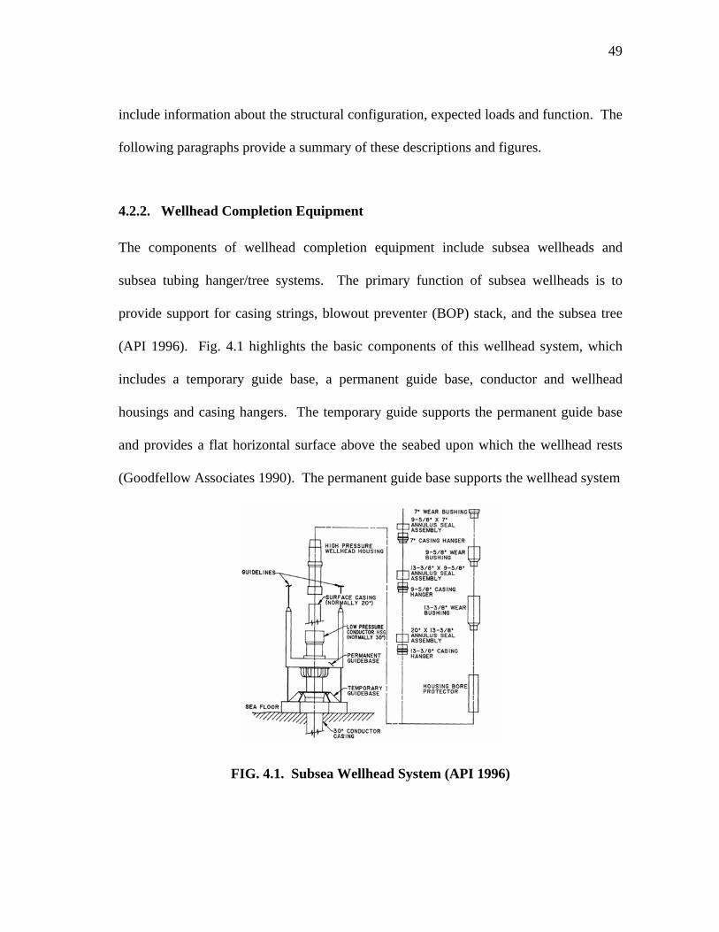
49

include information about the structural configuration, expected loads and function. The

following paragraphs provide a summary of these descriptions and figures.

4.2.2. Wellhead Completion Equipment

The components of wellhead completion equipment include subsea wellheads and

subsea tubing hanger/tree systems. The primary function of subsea wellheads is to

provide support for casing strings, blowout preventer (BOP) stack, and the subsea tree

(API 1996). Fig. 4.1 highlights the basic components of this wellhead system, which

includes a temporary guide base, a permanent guide base, conductor and wellhead

housings and casing hangers. The temporary guide supports the permanent guide base

and provides a flat horizontal surface above the seabed upon which the wellhead rests

(Goodfellow Associates 1990). The permanent guide base supports the wellhead system

FIG. 4.1. Subsea Wellhead System (API 1996)

50

and acts as a template for the placement of the BOP stack and subsea tree. The casing

hangers are used to support casing strings inside the wellhead. The conductor housing

attaches to the permanent guide base and extends down to attach to the conductor casing

and the wellhead housing, which fits inside the conductor housing, and maintains

constant pressure inside the well.

As shown in Fig. 4.2, the subsea tubing hanger system provides support for the tubing

inside the wellhead and maintains pressure between the tubing and the wellhead. Subsea

Christmas trees control the flow for production and injection wells through a series of

valves (see Fig. 4.3) (Goodfellow Associates 1990). These structures can be installed in

remote locations in order to retrieve resources from “marginal fields” or can be installed

with templates to aid with retrieval and production in locations where the oil reserves are

large.

Structural design considerations for these systems include soil-structure interaction,

environmental loads such as earthquake and current, thermal loads, and externally

applied loads originating from connecting pipelines and risers. The largest loads are

generated by the risers, applying moment and tension to the wellhead. The flowline

connections also provide a significant amount of loading in the form of shear and

applied moment. The subsea tubing hanger/wellhead connection is subjected to the

same loads as the wellhead systems (see Fig. 4.3).

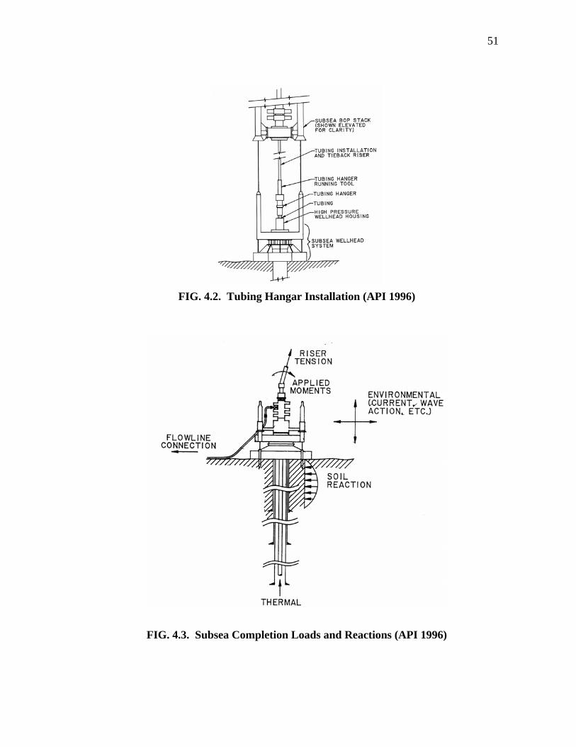
51

FIG. 4.2. Tubing Hangar Installation (API 1996)

FIG. 4.3. Subsea Completion Loads and Reactions (API 1996)

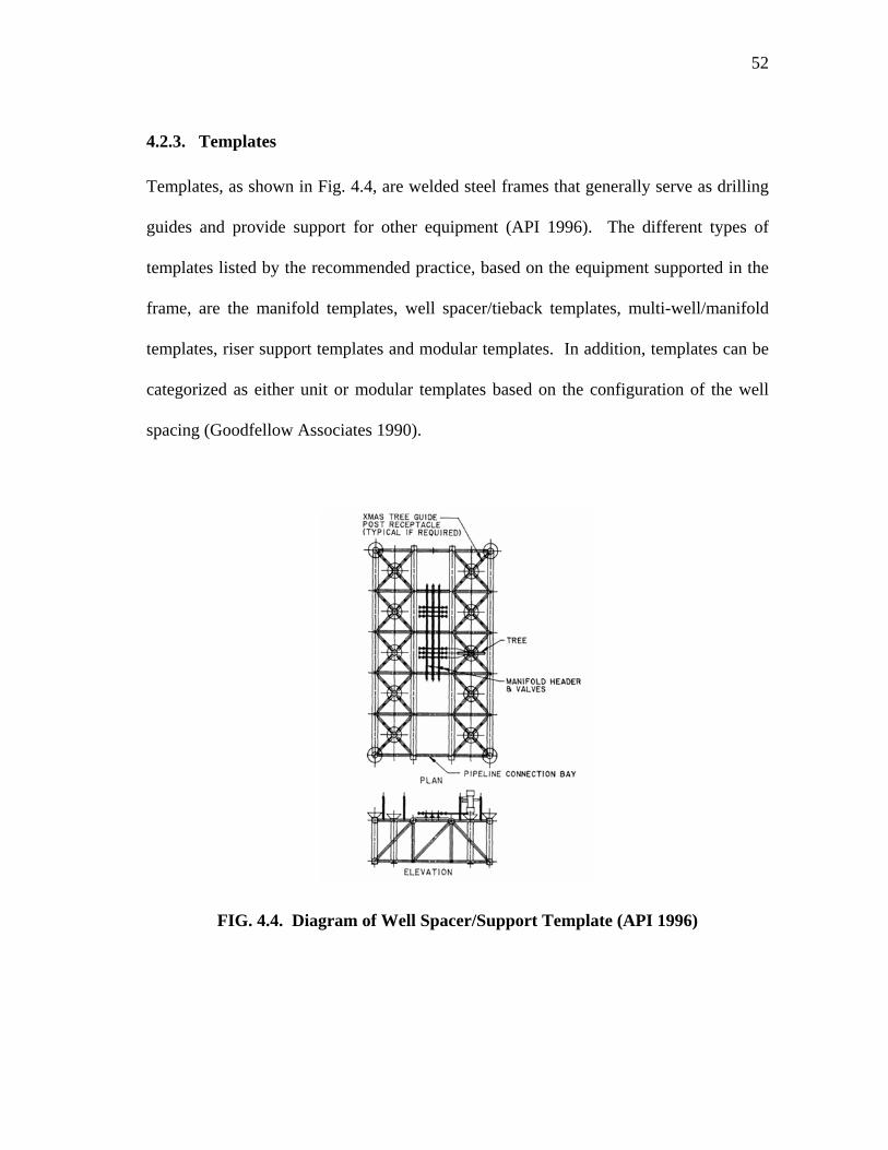
52

4.2.3. Templates

Templates, as shown in Fig. 4.4, are welded steel frames that generally serve as drilling

guides and provide support for other equipment (API 1996). The different types of

templates listed by the recommended practice, based on the equipment supported in the

frame, are the manifold templates, well spacer/tieback templates, multi-well/manifold

templates, riser support templates and modular templates. In addition, templates can be

categorized as either unit or modular templates based on the configuration of the well

spacing (Goodfellow Associates 1990).

FIG. 4.4. Diagram of Well Spacer/Support Template (API 1996)

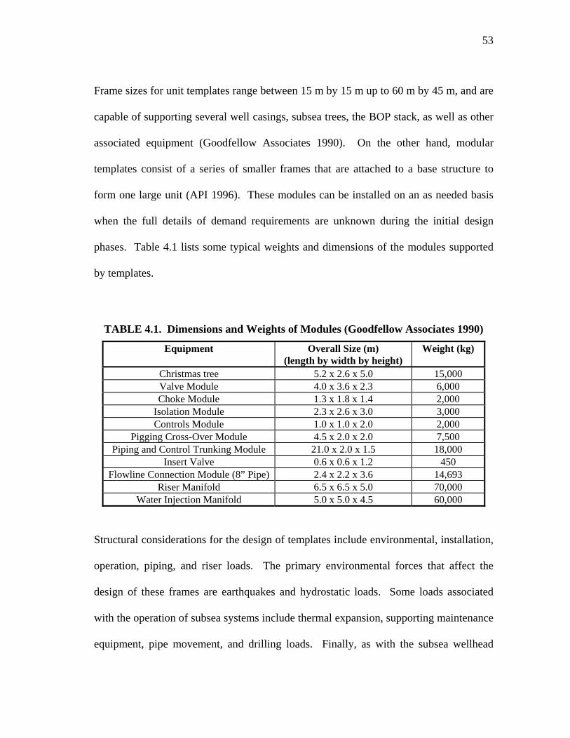
53

Frame sizes for unit templates range between 15 m by 15 m up to 60 m by 45 m, and are

capable of supporting several well casings, subsea trees, the BOP stack, as well as other

associated equipment (Goodfellow Associates 1990). On the other hand, modular

templates consist of a series of smaller frames that are attached to a base structure to

form one large unit (API 1996). These modules can be installed on an as needed basis

when the full details of demand requirements are unknown during the initial design

phases. Table 4.1 lists some typical weights and dimensions of the modules supported

by templates.

TABLE 4.1. Dimensions and Weights of Modules (Goodfellow Associates 1990)

Equipment Overall Size (m) (length by width by height)

Weight (kg)

Christmas tree 5.2 x 2.6 x 5.0 15,000 Valve Module 4.0 x 3.6 x 2.3 6,000 Choke Module 1.3 x 1.8 x 1.4 2,000

Isolation Module 2.3 x 2.6 x 3.0 3,000 Controls Module 1.0 x 1.0 x 2.0 2,000

Pigging Cross-Over Module 4.5 x 2.0 x 2.0 7,500 Piping and Control Trunking Module 21.0 x 2.0 x 1.5 18,000

Insert Valve 0.6 x 0.6 x 1.2 450 Flowline Connection Module (8” Pipe) 2.4 x 2.2 x 3.6 14,693

Riser Manifold 6.5 x 6.5 x 5.0 70,000 Water Injection Manifold 5.0 x 5.0 x 4.5 60,000

Structural considerations for the design of templates include environmental, installation,

operation, piping, and riser loads. The primary environmental forces that affect the

design of these frames are earthquakes and hydrostatic loads. Some loads associated

with the operation of subsea systems include thermal expansion, supporting maintenance

equipment, pipe movement, and drilling loads. Finally, as with the subsea wellhead

54

completion systems, the soil conditions play a critical role in the design of these

structures.

4.2.4. Manifold Systems

The primary function of a manifold system is to collect or distribute produced fluids.

Additional functions, such as well testing and servicing, may also be performed using

the manifold if the appropriate equipment is provided. The size and type of manifold

used for each application is dependent upon the number of wells located in each field

(Goodfellow Associates 1990). Some of the same loads used in template design are

applicable to the design of manifolds as well (API 1996). These loads may include

seismic effects and thermal expansion.

Template well manifolds and satellite well manifolds are two types of manifold systems

available for subsea applications (Goodfellow Associates 1990). The oil or gas is

collected from reservoirs or wells and distributed to riser lines by template manifolds. In

addition, these systems are responsible for injecting water back into the wells and

transmitting riser loads to the template, and providing a means of releasing the subsea

system from the risers in case of emergency. Satellite well manifolds are capable of

controlling the flow of fluids from reservoirs or wells.

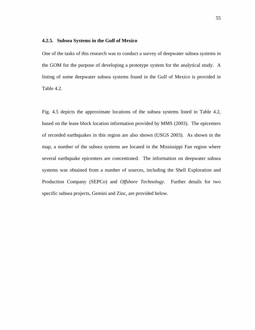
55

4.2.5. Subsea Systems in the Gulf of Mexico

One of the tasks of this research was to conduct a survey of deepwater subsea systems in

the GOM for the purpose of developing a prototype system for the analytical study. A

listing of some deepwater subsea systems found in the Gulf of Mexico is provided in

Table 4.2.

Fig. 4.5 depicts the approximate locations of the subsea systems listed in Table 4.2,

based on the lease block location information provided by MMS (2003). The epicenters

of recorded earthquakes in this region are also shown (USGS 2003). As shown in the

map, a number of the subsea systems are located in the Mississippi Fan region where

several earthquake epicenters are concentrated. The information on deepwater subsea

systems was obtained from a number of sources, including the Shell Exploration and

Production Company (SEPCo) and Offshore Technology. Further details for two

specific subsea projects, Gemini and Zinc, are provided below.

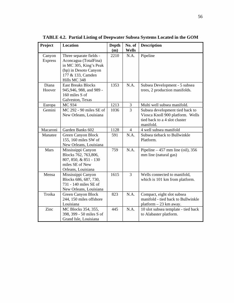
56

TABLE 4.2. Partial Listing of Deepwater Subsea Systems Located in the GOM

Project Location Depth(m)

No. of Wells

Description

Canyon Express

Three separate fields - Aconcagua (TotalFina) in MC 305, King’s Peak (bp) in Desoto Canyon 177 & 133, Camden Hills MC 348

2210 N.A. Pipeline

Diana Hoover

East Breaks Blocks 945,946, 988, and 989 - 160 miles S of Galveston, Texas

1353 N.A. Subsea Development - 5 subsea trees, 2 production manifolds.

Europa MC 934 1213 3 Multi well subsea manifold. Gemini

MC 292 - 90 miles SE of New Orleans, Louisiana

1036 3 Subsea development tied back to Viosca Knoll 900 platform. Wells tied back to a 4 slot cluster manifold.

Macaroni Garden Banks 602 1128 4 4 well subsea manifold Manatee Green Canyon Block

155, 160 miles SW of New Orleans, Louisiana

591 N.A. Subsea tieback to Bullwinkle Platform.

Mars Mississippi Canyon Blocks 762, 763,806, 807, 850, & 851 - 130 miles SE of New Orleans, Louisiana

759 N.A. Pipeline – 457 mm line (oil), 356 mm line (natural gas)

Mensa Mississippi Canyon Blocks 686, 687, 730, 731 - 140 miles SE of New Orleans, Louisiana

1615 3 Wells connected to manifold, which is 101 km from platform.

Troika Green Canyon Block 244, 150 miles offshore Louisiana

823 N.A. Compact, eight slot subsea manifold - tied back to Bullwinkle platform – 23 km away.

Zinc MC Blocks 354, 355, 398, 399 - 50 miles S of Grand Isle, Louisiana

445 N.A. 10 slot subsea template - tied back to Alabaster platform.

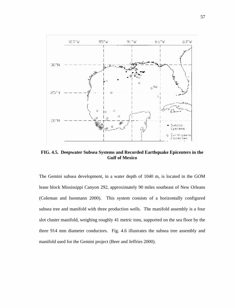
57

FIG. 4.5. Deepwater Subsea Systems and Recorded Earthquake Epicenters in the Gulf of Mexico

The Gemini subsea development, in a water depth of 1040 m, is located in the GOM

lease block Mississippi Canyon 292, approximately 90 miles southeast of New Orleans

(Coleman and Isenmann 2000). This system consists of a horizontally configured

subsea tree and manifold with three production wells. The manifold assembly is a four

slot cluster manifold, weighing roughly 41 metric tons, supported on the sea floor by the

three 914 mm diameter conductors. Fig. 4.6 illustrates the subsea tree assembly and

manifold used for the Gemini project (Beer and Jeffries 2000).

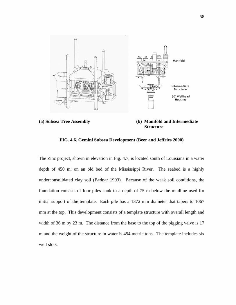
58

(a) Subsea Tree Assembly (b) Manifold and Intermediate Structure

FIG. 4.6. Gemini Subsea Development (Beer and Jeffries 2000)

The Zinc project, shown in elevation in Fig. 4.7, is located south of Louisiana in a water

depth of 450 m, on an old bed of the Mississippi River. The seabed is a highly

underconsolidated clay soil (Bednar 1993). Because of the weak soil conditions, the

foundation consists of four piles sunk to a depth of 75 m below the mudline used for

initial support of the template. Each pile has a 1372 mm diameter that tapers to 1067

mm at the top. This development consists of a template structure with overall length and

width of 36 m by 23 m. The distance from the base to the top of the pigging valve is 17

m and the weight of the structure in water is 454 metric tons. The template includes six

well slots.

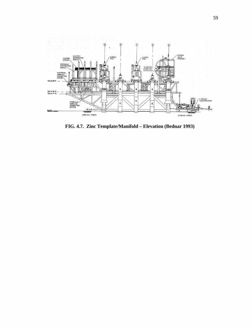
59

FIG. 4.7. Zinc Template/Manifold – Elevation (Bednar 1993)

60

5. STRUCTURAL MODELS AND ANALYSIS PROCEDURES

5.1. INTRODUCTION

The previous section contained a general description of the various types and functions

of subsea systems and highlighted a few deepwater systems in the Gulf of Mexico. This

section presents the details of a selected prototype subsea system, the development of

the numerical model of this system, and the parametric study. The final section of this

section outlines the details of the analysis procedures used to evaluate these systems.

5.2. DESCRIPTION OF ANALYTICAL MODEL

5.2.1. Prototype Structure

One of the objectives for this research was to identify a prototype subsea system to

evaluate the expected performance of subsea systems in the Gulf of Mexico under

seismic loading. Although each subsea system is designed to meet the site and

performance requirements, the basic geometry, structural member sizing, and loads are

similar for each system type. The most significant differences are observed in the

templates, manifolds, subsea wellheads and subsea trees. However, the foundation

support system tends to be similar among subsea systems, such that a prototype for an

analytical study may be defined.

The prototype system chosen for this study was derived from a Kvaerner advertisement

for a single wellhead subsea Christmas tree in a trade magazine (see Fig. 5.1) (Kvaerner

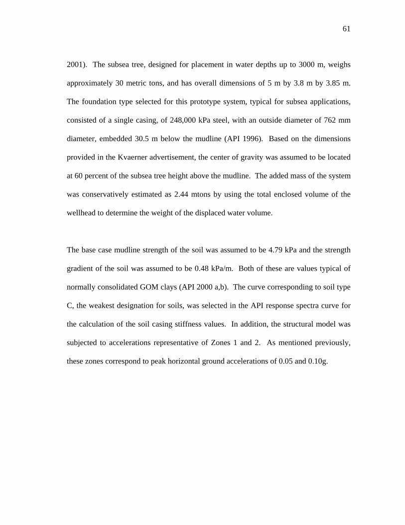
61

2001). The subsea tree, designed for placement in water depths up to 3000 m, weighs

approximately 30 metric tons, and has overall dimensions of 5 m by 3.8 m by 3.85 m.

The foundation type selected for this prototype system, typical for subsea applications,

consisted of a single casing, of 248,000 kPa steel, with an outside diameter of 762 mm

diameter, embedded 30.5 m below the mudline (API 1996). Based on the dimensions

provided in the Kvaerner advertisement, the center of gravity was assumed to be located

at 60 percent of the subsea tree height above the mudline. The added mass of the system

was conservatively estimated as 2.44 mtons by using the total enclosed volume of the

wellhead to determine the weight of the displaced water volume.

The base case mudline strength of the soil was assumed to be 4.79 kPa and the strength

gradient of the soil was assumed to be 0.48 kPa/m. Both of these are values typical of

normally consolidated GOM clays (API 2000 a,b). The curve corresponding to soil type

C, the weakest designation for soils, was selected in the API response spectra curve for

the calculation of the soil casing stiffness values. In addition, the structural model was

subjected to accelerations representative of Zones 1 and 2. As mentioned previously,

these zones correspond to peak horizontal ground accelerations of 0.05 and 0.10g.

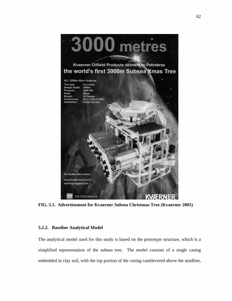
62

FIG. 5.1. Advertisement for Kvaerner Subsea Christmas Tree (Kvaerner 2001)

5.2.2. Baseline Analytical Model

The analytical model used for this study is based on the prototype structure, which is a

simplified representation of the subsea tree. The model consists of a single casing

embedded in clay soil, with the top portion of the casing cantilevered above the mudline,

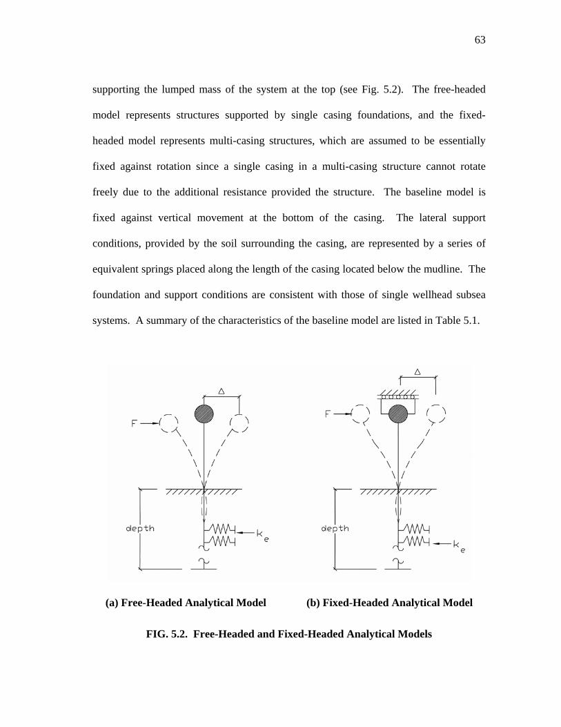
63

supporting the lumped mass of the system at the top (see Fig. 5.2). The free-headed

model represents structures supported by single casing foundations, and the fixed-

headed model represents multi-casing structures, which are assumed to be essentially

fixed against rotation since a single casing in a multi-casing structure cannot rotate

freely due to the additional resistance provided the structure. The baseline model is

fixed against vertical movement at the bottom of the casing. The lateral support

conditions, provided by the soil surrounding the casing, are represented by a series of

equivalent springs placed along the length of the casing located below the mudline. The

foundation and support conditions are consistent with those of single wellhead subsea

systems. A summary of the characteristics of the baseline model are listed in Table 5.1.

(a) Free-Headed Analytical Model (b) Fixed-Headed Analytical Model

FIG. 5.2. Free-Headed and Fixed-Headed Analytical Models

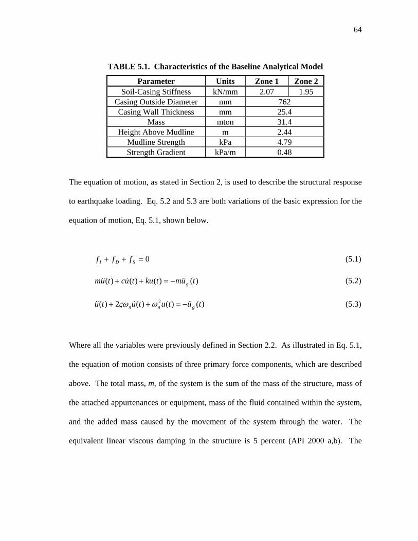
64

TABLE 5.1. Characteristics of the Baseline Analytical Model

Parameter Units Zone 1 Zone 2 Soil-Casing Stiffness kN/mm 2.07 1.95

Casing Outside Diameter mm 762 Casing Wall Thickness mm 25.4

Mass mton 31.4 Height Above Mudline m 2.44

Mudline Strength kPa 4.79 Strength Gradient kPa/m 0.48

The equation of motion, as stated in Section 2, is used to describe the structural response

to earthquake loading. Eq. 5.2 and 5.3 are both variations of the basic expression for the

equation of motion, Eq. 5.1, shown below.

0=++ SDI fff (5.1)

)()()()( tumtkutuctum g&&&&& −=++ (5.2)

)()()(2)( 2 tutututu gnn &&&&& −=++ ωςω (5.3)

Where all the variables were previously defined in Section 2.2. As illustrated in Eq. 5.1,

the equation of motion consists of three primary force components, which are described

above. The total mass, m, of the system is the sum of the mass of the structure, mass of

the attached appurtenances or equipment, mass of the fluid contained within the system,

and the added mass caused by the movement of the system through the water. The

equivalent linear viscous damping in the structure is 5 percent (API 2000 a,b). The

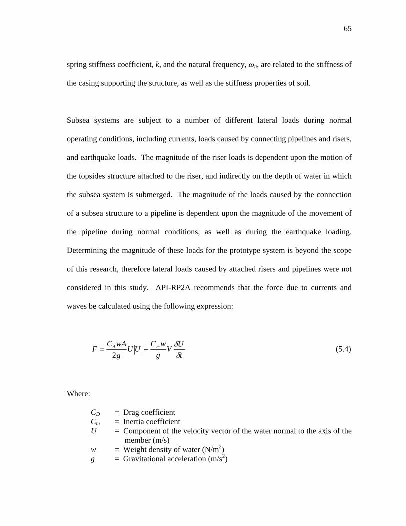
65

spring stiffness coefficient, k, and the natural frequency, ωn, are related to the stiffness of

the casing supporting the structure, as well as the stiffness properties of soil.

Subsea systems are subject to a number of different lateral loads during normal

operating conditions, including currents, loads caused by connecting pipelines and risers,

and earthquake loads. The magnitude of the riser loads is dependent upon the motion of

the topsides structure attached to the riser, and indirectly on the depth of water in which

the subsea system is submerged. The magnitude of the loads caused by the connection

of a subsea structure to a pipeline is dependent upon the magnitude of the movement of

the pipeline during normal conditions, as well as during the earthquake loading.

Determining the magnitude of these loads for the prototype system is beyond the scope

of this research, therefore lateral loads caused by attached risers and pipelines were not

considered in this study. API-RP2A recommends that the force due to currents and

waves be calculated using the following expression:

tUV

gwC

UUgwAC

F md

δδ

+=2

(5.4)

Where:

CD = Drag coefficient Cm = Inertia coefficient U = Component of the velocity vector of the water normal to the axis of the member (m/s) w = Weight density of water (N/m2) g = Gravitational acceleration (m/s2)

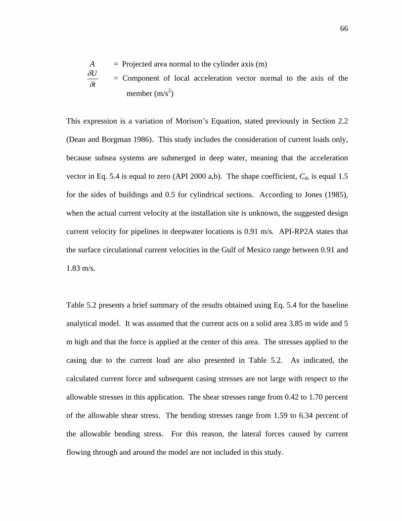
66

A = Projected area normal to the cylinder axis (m)

t

Uδ

δ = Component of local acceleration vector normal to the axis of the

member (m/s2)

This expression is a variation of Morison’s Equation, stated previously in Section 2.2

(Dean and Borgman 1986). This study includes the consideration of current loads only,

because subsea systems are submerged in deep water, meaning that the acceleration

vector in Eq. 5.4 is equal to zero (API 2000 a,b). The shape coefficient, Cd, is equal 1.5

for the sides of buildings and 0.5 for cylindrical sections. According to Jones (1985),

when the actual current velocity at the installation site is unknown, the suggested design

current velocity for pipelines in deepwater locations is 0.91 m/s. API-RP2A states that

the surface circulational current velocities in the Gulf of Mexico range between 0.91 and

1.83 m/s.

Table 5.2 presents a brief summary of the results obtained using Eq. 5.4 for the baseline

analytical model. It was assumed that the current acts on a solid area 3.85 m wide and 5

m high and that the force is applied at the center of this area. The stresses applied to the

casing due to the current load are also presented in Table 5.2. As indicated, the

calculated current force and subsequent casing stresses are not large with respect to the

allowable stresses in this application. The shear stresses range from 0.42 to 1.70 percent

of the allowable shear stress. The bending stresses range from 1.59 to 6.34 percent of

the allowable bending stress. For this reason, the lateral forces caused by current

flowing through and around the model are not included in this study.

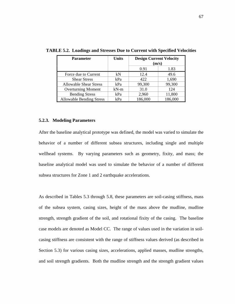
67

TABLE 5.2. Loadings and Stresses Due to Current with Specified Velocities

Design Current Velocity (m/s)

Parameter Units

0.91 1.83 Force due to Current kN 12.4 49.6

Shear Stress kPa 422 1,690 Allowable Shear Stress kPa 99,300 99,300 Overturning Moment kN-m 31.0 124

Bending Stress kPa 2,960 11,800 Allowable Bending Stress kPa 186,000 186,000

5.2.3. Modeling Parameters

After the baseline analytical prototype was defined, the model was varied to simulate the

behavior of a number of different subsea structures, including single and multiple

wellhead systems. By varying parameters such as geometry, fixity, and mass; the

baseline analytical model was used to simulate the behavior of a number of different

subsea structures for Zone 1 and 2 earthquake accelerations.

As described in Tables 5.3 through 5.8, these parameters are soil-casing stiffness, mass

of the subsea system, casing sizes, height of the mass above the mudline, mudline

strength, strength gradient of the soil, and rotational fixity of the casing. The baseline

case models are denoted as Model CC. The range of values used in the variation in soil-

casing stiffness are consistent with the range of stiffness values derived (as described in

Section 5.3) for various casing sizes, accelerations, applied masses, mudline strengths,

and soil strength gradients. Both the mudline strength and the strength gradient values

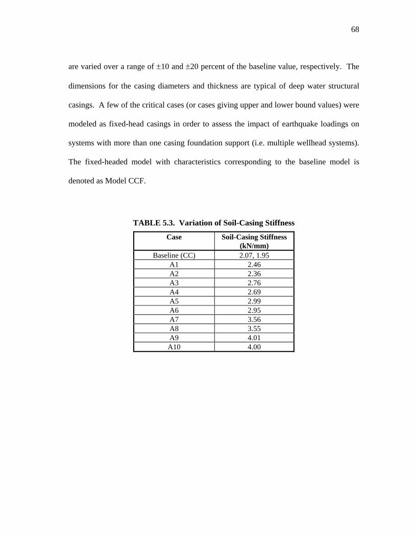
68

are varied over a range of ±10 and ±20 percent of the baseline value, respectively. The

dimensions for the casing diameters and thickness are typical of deep water structural

casings. A few of the critical cases (or cases giving upper and lower bound values) were

modeled as fixed-head casings in order to assess the impact of earthquake loadings on

systems with more than one casing foundation support (i.e. multiple wellhead systems).

The fixed-headed model with characteristics corresponding to the baseline model is

denoted as Model CCF.

TABLE 5.3. Variation of Soil-Casing Stiffness

Case Soil-Casing Stiffness (kN/mm)

Baseline (CC) 2.07, 1.95 A1 2.46 A2 2.36 A3 2.76 A4 2.69 A5 2.99 A6 2.95 A7 3.56 A8 3.55 A9 4.01

A10 4.00

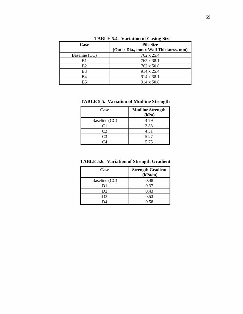
69

TABLE 5.4. Variation of Casing Size Case Pile Size

(Outer Dia., mm x Wall Thickness, mm) Baseline (CC) 762 x 25.4

B1 762 x 38.1 B2 762 x 50.8 B3 914 x 25.4 B4 914 x 38.1 B5 914 x 50.8

TABLE 5.5. Variation of Mudline Strength

Case Mudline Strength (kPa)

Baseline (CC) 4.79 C1 3.83 C2 4.31 C3 5.27 C4 5.75

TABLE 5.6. Variation of Strength Gradient

Case Strength Gradient (kPa/m)

Baseline (CC) 0.48 D1 0.37 D2 0.43 D3 0.53 D4 0.58

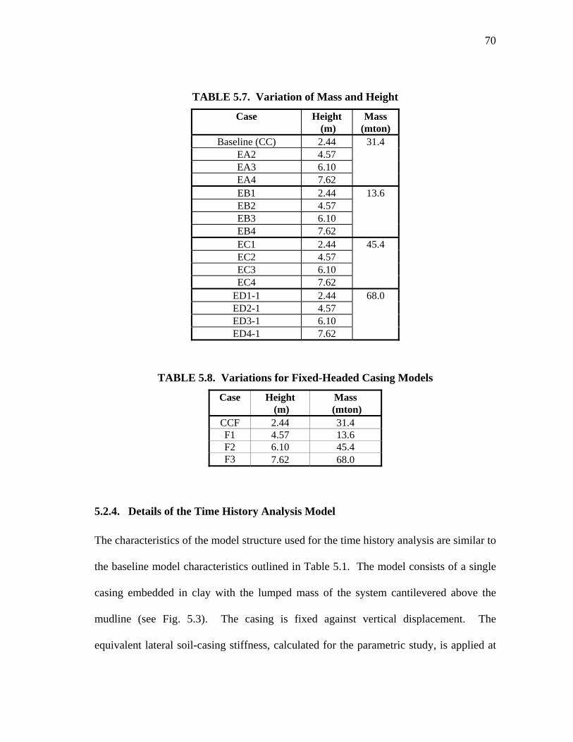
70

TABLE 5.7. Variation of Mass and Height

Case Height (m)

Mass (mton)

Baseline (CC) 2.44 EA2 4.57 EA3 6.10 EA4 7.62

31.4

EB1 2.44 EB2 4.57 EB3 6.10 EB4 7.62

13.6

EC1 2.44 EC2 4.57 EC3 6.10 EC4 7.62

45.4

ED1-1 2.44 ED2-1 4.57 ED3-1 6.10 ED4-1 7.62

68.0

TABLE 5.8. Variations for Fixed-Headed Casing Models

Case Height (m)

Mass (mton)

CCF 2.44 31.4 F1 4.57 13.6 F2 6.10 45.4 F3 7.62 68.0

5.2.4. Details of the Time History Analysis Model

The characteristics of the model structure used for the time history analysis are similar to

the baseline model characteristics outlined in Table 5.1. The model consists of a single

casing embedded in clay with the lumped mass of the system cantilevered above the

mudline (see Fig. 5.3). The casing is fixed against vertical displacement. The

equivalent lateral soil-casing stiffness, calculated for the parametric study, is applied at

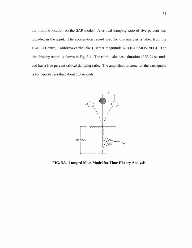
71

the mudline location on the SAP model. A critical damping ratio of five percent was

included in the input. The acceleration record used for this analysis is taken from the

1940 El Centro, California earthquake (Richter magnitude 6.9) (COSMOS 2003). The

time history record is shown in Fig. 5.4. The earthquake has a duration of 53.74 seconds

and has a five percent critical damping ratio. The amplification zone for the earthquake

is for periods less than about 1.0 seconds.

FIG. 5.3. Lumped Mass Model for Time History Analysis

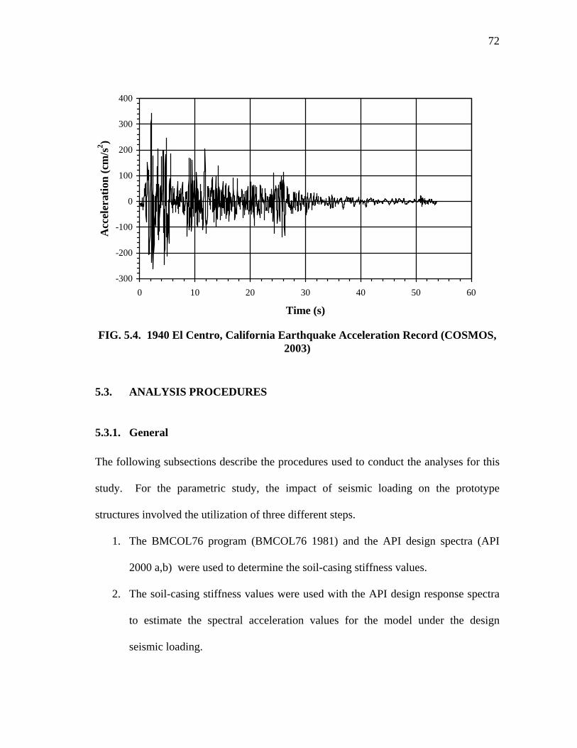
72

-300

-200

-100

0

100

200

300

400

0 10 20 30 40 50 6

Time (s)

Acc

eler

atio

n (c

m/s2 )

0

FIG. 5.4. 1940 El Centro, California Earthquake Acceleration Record (COSMOS,

2003)

5.3. ANALYSIS PROCEDURES

5.3.1. General

The following subsections describe the procedures used to conduct the analyses for this

study. For the parametric study, the impact of seismic loading on the prototype

structures involved the utilization of three different steps.

1. The BMCOL76 program (BMCOL76 1981) and the API design spectra (API

2000 a,b) were used to determine the soil-casing stiffness values.

2. The soil-casing stiffness values were used with the API design response spectra

to estimate the spectral acceleration values for the model under the design

seismic loading.

73

3. The force and displacement values were obtained using the response spectra

method.

4. The force values were used to calculate the stresses in the casing and deflection

of the model for the design seismic loading.

For the time history analysis, the following steps were used:

1. The soil casing stiffness for the baseline model was obtained from the parametric

study.

2. A time history analysis was conducted for the baseline model using the SAP2000

program (SAP2000 1999).

3. The force values obtained from the SAP2000 output were used to calculate the

stresses in the casing. The deflection values were also obtained from the output.

5.3.2. Calculation of Equivalent Soil-Casing Stiffness

The first step of the analysis was to determine the soil casing stiffness values for the

model. The BMCOL76 program (BMCOL76 1981) computes deflections and reactions

for an embedded casing (or pile) with specific geometry, loading conditions, and

nonlinear soil resistance values. In this program, the soil-pile relationship is modeled as

a beam-column on an inelastic foundation, which is detailed further in Section 2.2.3.

Because the lateral response of the soil-casing is nonlinear, a linearized secant stiffness

was determined using the design response spectra shown in Figure C2.3.6-2 of API-

RP2A for a specified zone and soil type (API 2000 a,b). As shown in Table 5.4, the soil

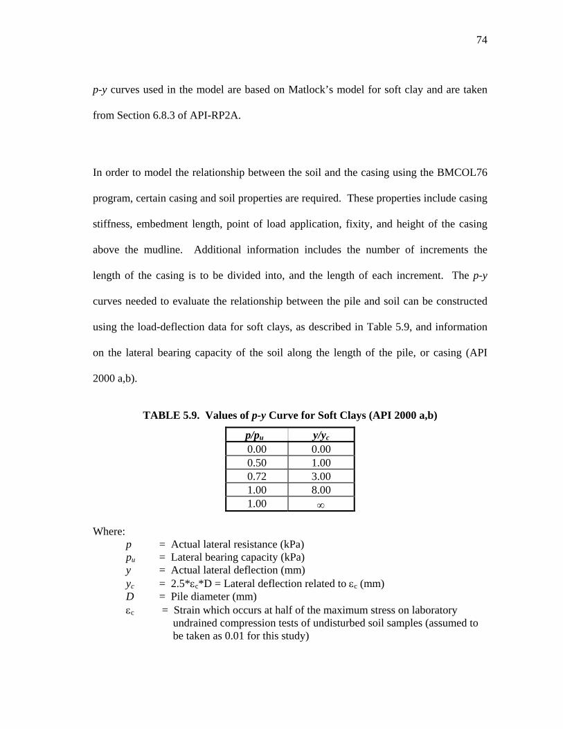
74

p-y curves used in the model are based on Matlock’s model for soft clay and are taken

from Section 6.8.3 of API-RP2A.

In order to model the relationship between the soil and the casing using the BMCOL76

program, certain casing and soil properties are required. These properties include casing

stiffness, embedment length, point of load application, fixity, and height of the casing

above the mudline. Additional information includes the number of increments the

length of the casing is to be divided into, and the length of each increment. The p-y

curves needed to evaluate the relationship between the pile and soil can be constructed

using the load-deflection data for soft clays, as described in Table 5.9, and information

on the lateral bearing capacity of the soil along the length of the pile, or casing (API

2000 a,b).

TABLE 5.9. Values of p-y Curve for Soft Clays (API 2000 a,b)

p/pu y/yc

0.00 0.00 0.50 1.00 0.72 3.00 1.00 8.00 1.00 ∞

Where: p = Actual lateral resistance (kPa) pu = Lateral bearing capacity (kPa) y = Actual lateral deflection (mm) yc = 2.5*εc*D = Lateral deflection related to εc (mm) D = Pile diameter (mm) εc = Strain which occurs at half of the maximum stress on laboratory undrained compression tests of undisturbed soil samples (assumed to be taken as 0.01 for this study)

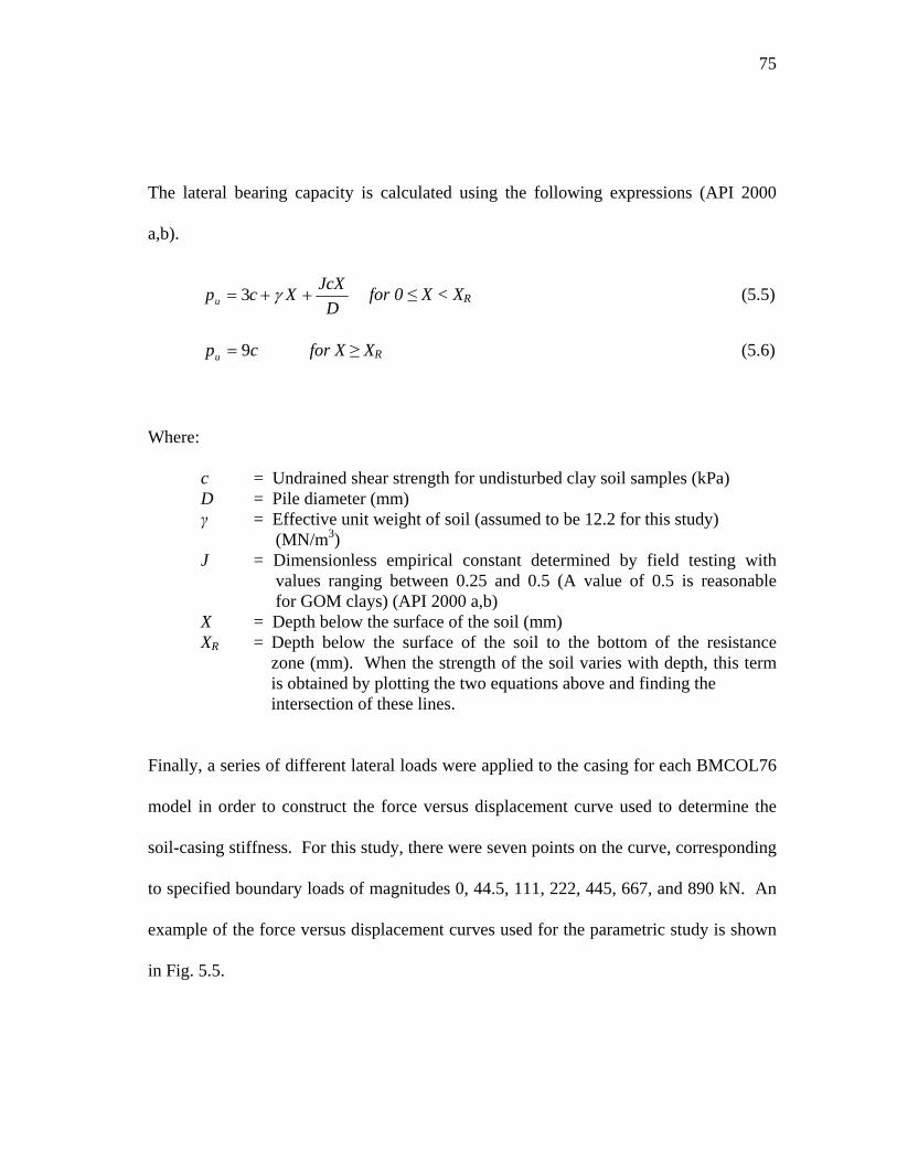
75

The lateral bearing capacity is calculated using the following expressions (API 2000

a,b).

DJcXXcpu ++= γ3 for 0 ≤ X < XR (5.5)

cpu 9= for X ≥ XR (5.6)

Where:

c = Undrained shear strength for undisturbed clay soil samples (kPa) D = Pile diameter (mm) γ = Effective unit weight of soil (assumed to be 12.2 for this study) (MN/m3) J = Dimensionless empirical constant determined by field testing with values ranging between 0.25 and 0.5 (A value of 0.5 is reasonable for GOM clays) (API 2000 a,b) X = Depth below the surface of the soil (mm) XR = Depth below the surface of the soil to the bottom of the resistance zone (mm). When the strength of the soil varies with depth, this term is obtained by plotting the two equations above and finding the intersection of these lines.

Finally, a series of different lateral loads were applied to the casing for each BMCOL76

model in order to construct the force versus displacement curve used to determine the

soil-casing stiffness. For this study, there were seven points on the curve, corresponding

to specified boundary loads of magnitudes 0, 44.5, 111, 222, 445, 667, and 890 kN. An

example of the force versus displacement curves used for the parametric study is shown

in Fig. 5.5.

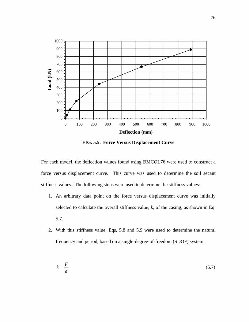
76

0

100

200

300

400

500

600

700

800

900

1000

0 100 200 300 400 500 600 700 800 900 1000

Deflection (mm)

Loa

d (k

N)

FIG. 5.5. Force Versus Displacement Curve

For each model, the deflection values found using BMCOL76 were used to construct a

force versus displacement curve. This curve was used to determine the soil secant

stiffness values. The following steps were used to determine the stiffness values:

1. An arbitrary data point on the force versus displacement curve was initially

selected to calculate the overall stiffness value, k, of the casing, as shown in Eq.

5.7.

2. With this stiffness value, Eqs. 5.8 and 5.9 were used to determine the natural

frequency and period, based on a single-degree-of-freedom (SDOF) system.

dFk = (5.7)

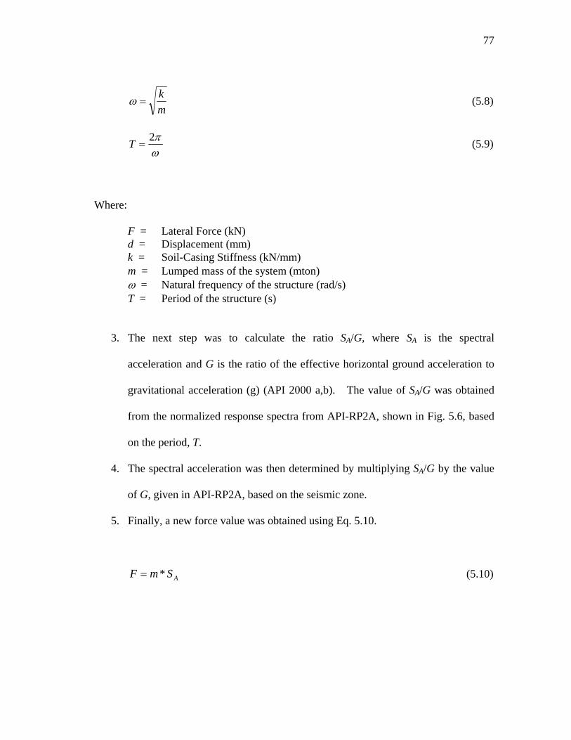
77

mk

=ω (5.8)

ωπ2

=T (5.9)

Where:

F = Lateral Force (kN) d = Displacement (mm) k = Soil-Casing Stiffness (kN/mm) m = Lumped mass of the system (mton) ω = Natural frequency of the structure (rad/s) T = Period of the structure (s)

3. The next step was to calculate the ratio SA/G, where SA is the spectral

acceleration and G is the ratio of the effective horizontal ground acceleration to

gravitational acceleration (g) (API 2000 a,b). The value of SA/G was obtained

from the normalized response spectra from API-RP2A, shown in Fig. 5.6, based

on the period, T.

4. The spectral acceleration was then determined by multiplying SA/G by the value

of G, given in API-RP2A, based on the seismic zone.

5. Finally, a new force value was obtained using Eq. 5.10.

ASmF *= (5.10)

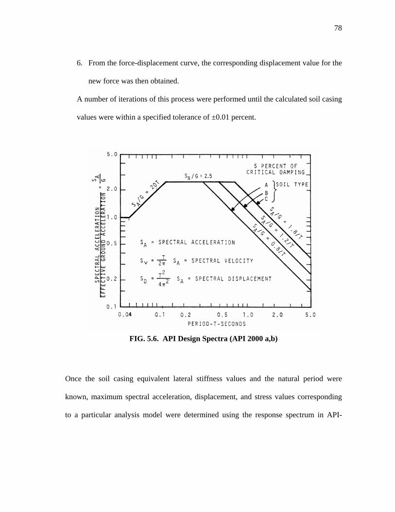
78

6. From the force-displacement curve, the corresponding displacement value for the

new force was then obtained.

A number of iterations of this process were performed until the calculated soil casing

values were within a specified tolerance of ±0.01 percent.

FIG. 5.6. API Design Spectra (API 2000 a,b)

Once the soil casing equivalent lateral stiffness values and the natural period were

known, maximum spectral acceleration, displacement, and stress values corresponding

to a particular analysis model were determined using the response spectrum in API-

79

RP2A (API 2000 a,b). The spectral acceleration, SA, of the system was calculated as

stated in the previous paragraph.

5.3.3. Time History Analysis Method

The SAP2000 analysis program was used to conduct the linear time history analysis for

this study (SAP2000 1999). The analytical model was constructed using most of the

same parameters used for the baseline analytical model in the parametric study (see

Sections 5.2.2 and 5.2.4). However, the lateral soil-casing stiffness value was derived

using the displacement of the casing at the mudline instead of the top of the casing

model. The resulting displacements and response of the structure were computed by the

SAP2000 program after the model information and a file containing the El Centro

earthquake acceleration record were defined. The SAP2000 program presents these

results in the form of data files that contain the accelerations for each time step in the

record. As with the parametric study, the shear forces were calculated by multiplying

the mass of the model by the acceleration values. The maximum moment and

displacement values corresponding to the maximum shear force were then obtained

using the BMCOL76 program.

5.3.4. Calculation of Force and Stress Values

The final step for the parametric study and time history analysis involved determining

the stresses and displacements that the casing of the model experiences under earthquake

80

loading. For the results, the maximum shear forces, overturning moments and

corresponding stresses were calculated to evaluate the performance of each model. This

evaluation also included determining the maximum displacement values for each model.

The shear forces, overturning moments, and stresses were calculated using Eqs. 5.11 to

5.13.

ASmF *= (5.11)

AFfv = (5.12)

IMcfb = (5.13)

Where:

F = Shear force (kN) SA = Spectral Acceleration (m/s2) fv = Shear stress (kPa) A = Area of structural element (m2) M = Overturning moment (kN-m) fb = Bending stress (kPa) I = Moment of inertia of structural element (mm4) c = Distance from extreme edge to the centroid of structural element (mm)

Because the length of the moment arm for the maximum overturning moment typically

occurred below the mudline, most of the moment and displacement values for the

models in the parametric study were obtained from the BMCOL76 program. However,

for models A1 to A10, where the soil-casing stiffness was varied independent of the

other model properties, obtaining the correct maximum moment and displacement values

81

using BMCOL76 program was more difficult. This is because there were several

different variations in soil and casing properties that could produce the designated

stiffness values. To approximate the maximum moment and displacement values for

these models, Eq. 5.14 and 5.15 were used.

AD STS 2

2

4π= (5.14)

dFM *= (5.15)

Where:

d = Length of the moment arm (m) T = Period of the casing (seconds)

Finally, the stresses obtained from these analyses were compared to the allowable

stresses, as defined by API-RP2A Working Stress Design for offshore structures (API

2000 a). An increase of 70 percent is permitted for the evaluation of stresses caused by

earthquake loading. In other words, the stresses caused by earthquake loading must be

less than or equal to 70 percent of the allowable stresses. The expressions used to

determine the allowable axial compressive stresses, shear stresses, and bending stresses

are as follows:

82

3

3

2

2

8)/(

8)/(33/5

2)/(1

cc

yc

a

CrKl

CrKl

FC

rKl

F−+

⎥⎦

⎤⎢⎣

⎡−

= for Kl/r < Cc (5.16)

2

2

)/(2312

rKlEFa

π= for Kl/r ≥ Cc (5.17)

yb FF 75.0= (5.18)

yv Ff 4.0= (5.19)

where:

Fa = Allowable axial stress (kPa) K = Effective length factor, defined as 1.0 for piles in API-RP2A l = Unbraced length of the member (m) r = Radius of gyration (m)

Cc = 05.

22⎥⎥⎦

⎤

⎢⎢⎣

⎡

yFEπ

Fy = Yield stress (kPa) Fb = Allowable bending stress (kPa) fv = Allowable shear stress (kPa)

Eq. 5.20 is used to determine the shear stress ratio (SSR). Since only the stresses

induced by earthquake loading are considered in this study, the SSR should be less than

or equal to 0.7.

7.0≤=v

vcal

ff

SSR (5.20)

83

Where:

fvcal = Calculated shear stress (kPa)

Eqs. 5.21 to 5.23 are used to calculate the combined axial and bending stress ratio (CSR)

for the casing. Since only the stresses caused by earthquake loading are considered in

this study, the CSR must be less than or equal to 0.7. According to API-RP2A,

cylindrical members should be designed to satisfy the expressions in Eqs. 5.21 and 5.22.

However, Eq. 5.23 can be substituted for these two expressions when the ratio of the

axial stress to the allowable axial stress is less than or equal to 0.15.

7.0)1(

22

≤

′−

++=

be

a

bybxm

a

a

FFf

ffC

Ff

CSR (5.21)

7.06.0

22

≤+

+=b

bybx

y

a

F

ff

Ff

CSR (5.22)

7.022

≤+

+=b

bybx

a

a

Fff

FfCSR for 15.0≤

a

a

Ff

(5.23)

Where:

Fa = Allowable axial stress (kPa) K = Effective length factor, defined as 1.0 for piles in API-RP2A l = Unbraced length of the member (m) r = Radius of gyration (m) CSR = Combined stress ratio

84

6. ANALYTICAL RESULTS

6.1. INTRODUCTION

The results from the parametric study and the time history analysis are presented in this

section. The results generated from the baseline analytical model are presented first,

followed by the results of the parametric study (for the free-headed casing models) from

varying the soil casing stiffness, casing size, mudline strength and strength gradient of

the soil, mass height above the mudline, and mass, respectively. In addition, the results

for the fixed-headed casing models are presented. A summary of the parametric study

results are presented in Section 6.2.9. Finally, the time history analysis results are

presented in Section 6.3.

6.2. PARAMETRIC STUDY

6.2.1. Results for the Baseline Model

Table 6.1 presents the data obtained from the analysis of the baseline prototype model.

The properties of this model, labeled as model CC, are based on the properties of the

selected prototype structure and typical site conditions in the GOM. The calculations

performed to obtain this data are presented in Appendix A.

The calculated period for the Zone 1 subsea model is approximately four percent less

than the period obtained from the Zone 2 model. As expected, the displacement and

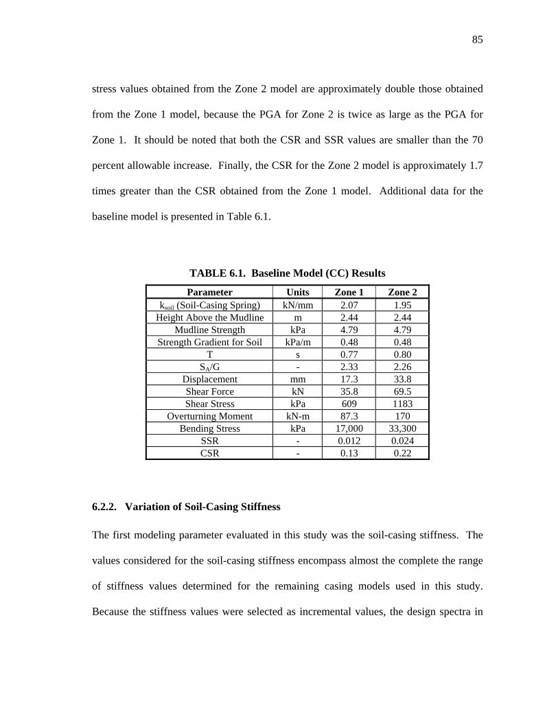
85

stress values obtained from the Zone 2 model are approximately double those obtained

from the Zone 1 model, because the PGA for Zone 2 is twice as large as the PGA for

Zone 1. It should be noted that both the CSR and SSR values are smaller than the 70

percent allowable increase. Finally, the CSR for the Zone 2 model is approximately 1.7

times greater than the CSR obtained from the Zone 1 model. Additional data for the

baseline model is presented in Table 6.1.

TABLE 6.1. Baseline Model (CC) Results

Parameter Units Zone 1 Zone 2 ksoil (Soil-Casing Spring) kN/mm 2.07 1.95

Height Above the Mudline m 2.44 2.44 Mudline Strength kPa 4.79 4.79

Strength Gradient for Soil kPa/m 0.48 0.48 T s 0.77 0.80

SA/G - 2.33 2.26 Displacement mm 17.3 33.8 Shear Force kN 35.8 69.5 Shear Stress kPa 609 1183

Overturning Moment kN-m 87.3 170 Bending Stress kPa 17,000 33,300

SSR - 0.012 0.024 CSR - 0.13 0.22

6.2.2. Variation of Soil-Casing Stiffness

The first modeling parameter evaluated in this study was the soil-casing stiffness. The

values considered for the soil-casing stiffness encompass almost the complete the range

of stiffness values determined for the remaining casing models used in this study.

Because the stiffness values were selected as incremental values, the design spectra in

86

API-RP2A (API 2000 a,b) was used only to calculate the displacements and stresses (see

Section 5). For these cases only, the maximum bending moment is calculated using a

moment arm distance which extends from the mudline to the center of gravity of the

mass.

The results obtained from varying the soil-casing stiffness values are presented in Tables

6.2 and 6.3. The relationship between stresses, displacements and periods with respect

to changes in the stiffness values are shown graphically in Figs. 6.1 to 6.4. As expected,

the period of the casing model decreases nonlinearly as the stiffness parameter increases.

In addition, there is a similar nonlinear relationship between the soil-casing stiffness and

observed displacements. However, Figs. 6.3 and 6.4 show that the shear and bending

stresses increase until the stiffness value is approximately 2.63 kN/mm or greater, at

which point there is no change in either shear or bending stresses. This indicates that an

increase in the stiffness parameter beyond this point will not cause a significant change

in the bending and shear stress values. Finally the CSR values for this variable ranged

between 0.06 and 0.13.

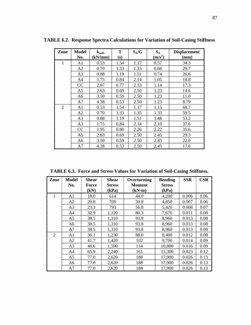
87

TABLE 6.2. Response Spectra Calculations for Variation of Soil-Casing Stiffness

Zone Model No.

ksoil, (kN/mm)

T (s)

SA/G SA (m/s2)

Displacement (mm)

A1 0.53 1.54 1.17 0.57 34.3 A2 0.70 1.33 1.35 0.66 29.7 A3 0.88 1.19 1.51 0.74 26.6 A4 1.75 0.84 2.14 1.05 18.8 CC 2.07 0.77 2.33 1.14 17.3 A5 2.63 0.69 2.50 1.23 14.6 A6 3.50 0.59 2.50 1.23 11.0

1

A7 4.38 0.53 2.50 1.23 8.79 A1 0.53 1.54 1.17 1.15 68.7 A2 0.70 1.33 1.35 1.33 59.5 A3 0.88 1.19 1.51 1.48 53.2 A3 1.75 0.84 2.14 2.10 37.6 CC 1.95 0.80 2.26 2.22 35.6 A5 2.63 0.69 2.50 2.45 29.3 A6 3.50 0.59 2.50 2.45 22.0

2

A7 4.38 0.53 2.50 2.45 17.6

TABLE 6.3. Force and Stress Values for Variation of Soil-Casing Stiffness.

Zone Model No.

Shear Force (kN)

Shear Stress (kPa)

Overturning Moment (kN-m)

Bending Stress (kPa)

SSR CSR

A1 18.0 614 44.0 4,200 0.006 0.06 A2 20.8 709 50.8 4,850 0.007 0.06 A3 23.3 793 56.8 5,420 0.008 0.07 A4 32.9 1,120 80.3 7,670 0.011 0.08 A5 38.5 1,310 93.8 8,960 0.013 0.08 A6 38.5 1,310 93.8 8,960 0.013 0.08

1

A7 38.5 1,310 93.8 8,960 0.013 0.08 A1 36.1 1,230 88.0 8,400 0.012 0.08 A2 41.7 1,420 102 9,700 0.014 0.09 A3 46.6 1,590 114 10,800 0.016 0.09 A4 65.9 2,240 161 15,300 0.023 0.12 A5 77.0 2,620 188 17,900 0.026 0.13 A6 77.0 2,620 188 17,900 0.026 0.13

2

A7 77.0 2,620 188 17,900 0.026 0.13

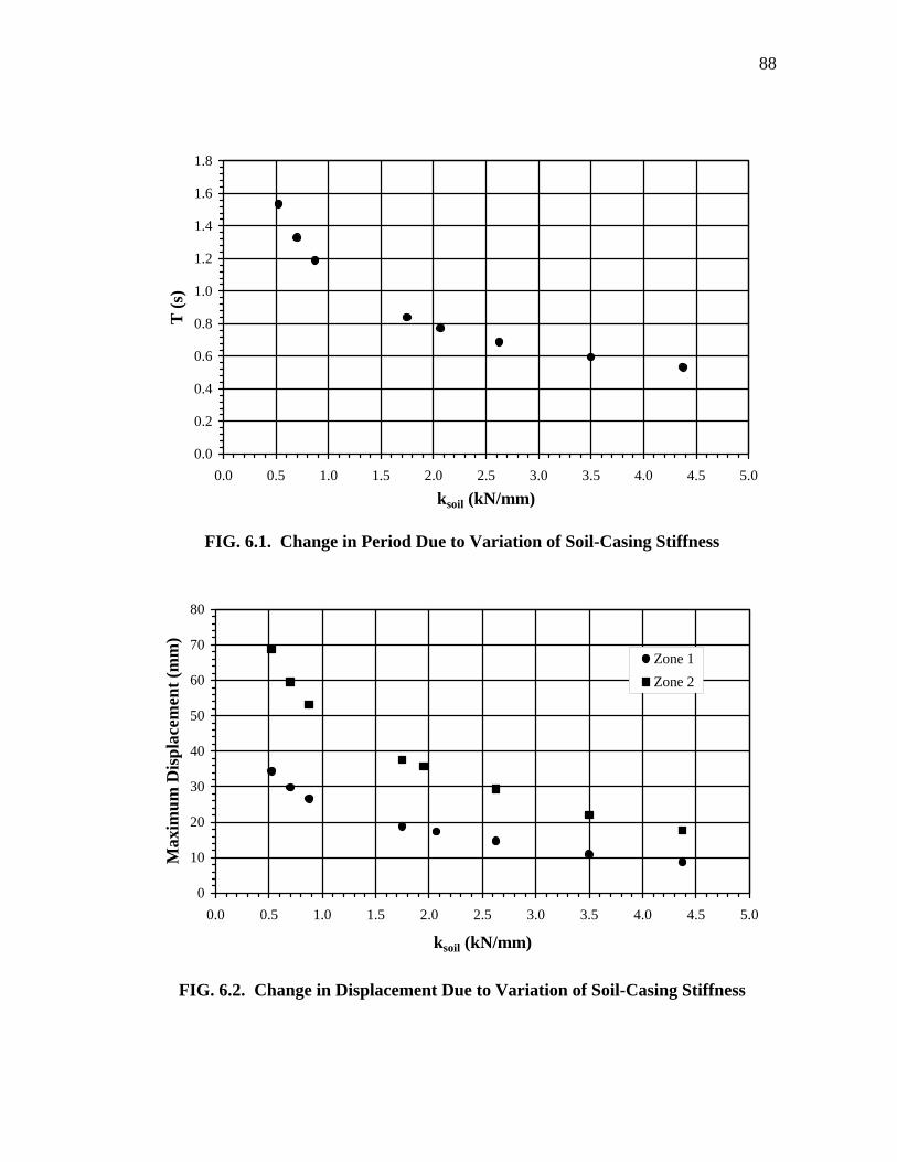
88

0.0

0.2

0.4

0.6

0.8

1.0

1.2

1.4

1.6

1.8

0.0 0.5 1.0 1.5 2.0 2.5 3.0 3.5 4.0 4.5 5.0

ksoil (kN/mm)

T (s

)

FIG. 6.1. Change in Period Due to Variation of Soil-Casing Stiffness

0

10

20

30

40

50

60

70

80

0.0 0.5 1.0 1.5 2.0 2.5 3.0 3.5 4.0 4.5 5.0

ksoil (kN/mm)

Max

imum

Dis

plac

emen

t (m

m)

Zone 1Zone 2

FIG. 6.2. Change in Displacement Due to Variation of Soil-Casing Stiffness

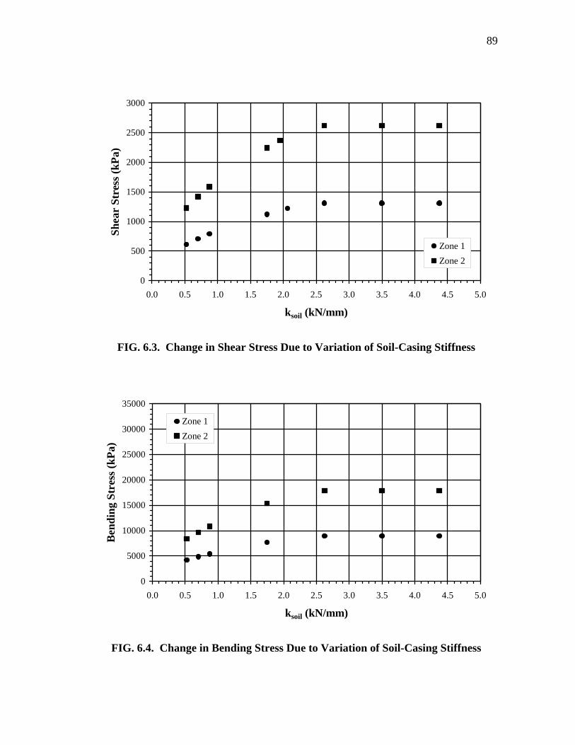
89

0

500

1000

1500

2000

2500

3000

0.0 0.5 1.0 1.5 2.0 2.5 3.0 3.5 4.0 4.5 5.0

ksoil (kN/mm)

Shea

r St

ress

(kPa

)

Zone 1Zone 2

FIG. 6.3. Change in Shear Stress Due to Variation of Soil-Casing Stiffness

0

5000

10000

15000

20000

25000

30000

35000

0.0 0.5 1.0 1.5 2.0 2.5 3.0 3.5 4.0 4.5 5.0

ksoil (kN/mm)

Ben

ding

Str

ess (

kPa)

Zone 1Zone 2

FIG. 6.4. Change in Bending Stress Due to Variation of Soil-Casing Stiffness

90

6.2.3. Variation of Casing Size

The dimensions chosen to evaluate the impact of varying casing size are consistent with

diameter and wall thicknesses typically used subsea pile applications. The soil-casing

stiffness values, maximum bending moments, and displacements were obtained using

the BMCOL76 analysis program, while the shear forces were calculated based on the

design spectra from API-RP2A (API 2000 a,b). Tables 6.4 and 6.5 present the results

obtained from the study for this parameter. The variation of period, displacement and

stress values with respect to the change in casing sizes are shown in Figs. 6.5 to 6.8.

As expected, the period, maximum tip deflection, and stress values decrease as the area

of steel increases. These values decrease because increasing the area of steel increases

the stiffness of the casing. There is approximately a 50 percent difference between the

shear and bending stress values obtained from the smallest and largest casing sizes.

Both the SSR and CSR values obtained for this parameter were less than 0.7. The SSR

values for the model B5, the largest casing size, are roughly 50 percent of those obtained

from the baseline model. The CSR values obtained for model B5 are approximately 45

percent less than the CSR values obtained for the baseline model.

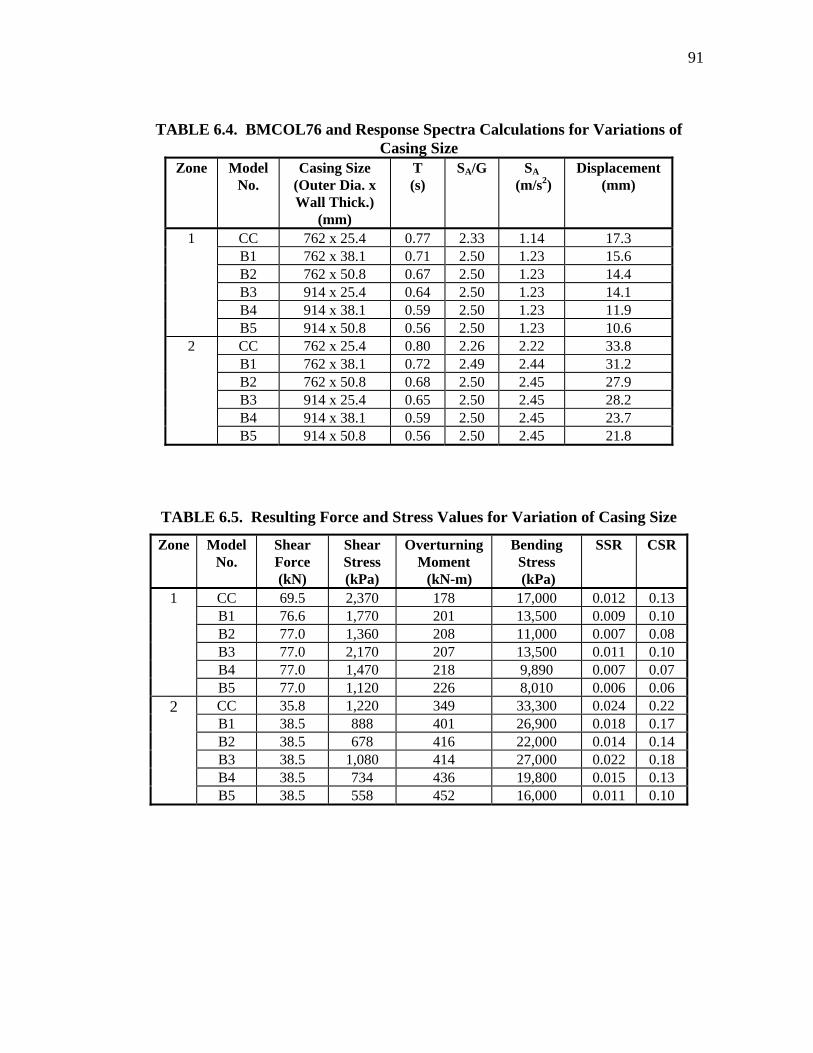
91

TABLE 6.4. BMCOL76 and Response Spectra Calculations for Variations of Casing Size

Zone Model No.

Casing Size (Outer Dia. x Wall Thick.)

(mm)

T (s)

SA/G SA (m/s2)

Displacement (mm)

CC 762 x 25.4 0.77 2.33 1.14 17.3 B1 762 x 38.1 0.71 2.50 1.23 15.6 B2 762 x 50.8 0.67 2.50 1.23 14.4 B3 914 x 25.4 0.64 2.50 1.23 14.1 B4 914 x 38.1 0.59 2.50 1.23 11.9

1

B5 914 x 50.8 0.56 2.50 1.23 10.6 CC 762 x 25.4 0.80 2.26 2.22 33.8 B1 762 x 38.1 0.72 2.49 2.44 31.2 B2 762 x 50.8 0.68 2.50 2.45 27.9 B3 914 x 25.4 0.65 2.50 2.45 28.2 B4 914 x 38.1 0.59 2.50 2.45 23.7

2

B5 914 x 50.8 0.56 2.50 2.45 21.8

TABLE 6.5. Resulting Force and Stress Values for Variation of Casing Size

Zone Model No.

Shear Force (kN)

Shear Stress (kPa)



SSR CSR

CC 69.5 2,370 178 17,000 0.012 0.13 B1 76.6 1,770 201 13,500 0.009 0.10 B2 77.0 1,360 208 11,000 0.007 0.08 B3 77.0 2,170 207 13,500 0.011 0.10 B4 77.0 1,470 218 9,890 0.007 0.07

1

B5 77.0 1,120 226 8,010 0.006 0.06 CC 35.8 1,220 349 33,300 0.024 0.22 B1 38.5 888 401 26,900 0.018 0.17 B2 38.5 678 416 22,000 0.014 0.14 B3 38.5 1,080 414 27,000 0.022 0.18 B4 38.5 734 436 19,800 0.015 0.13

2

B5 38.5 558 452 16,000 0.011 0.10

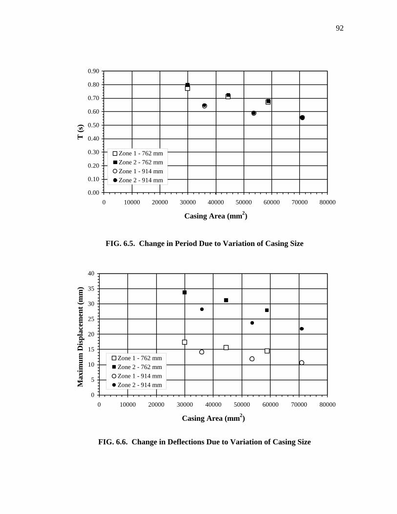
92

0.00

0.10

0.20

0.30

0.40

0.50

0.60

0.70

0.80

0.90

0 10000 20000 30000 40000 50000 60000 70000 80000

Casing Area (mm2)

T (s

)

Zone 1 - 762 mmZone 2 - 762 mmZone 1 - 914 mmZone 2 - 914 mm

FIG. 6.5. Change in Period Due to Variation of Casing Size

0

5

10

15

20

25

30

35

40

0 10000 20000 30000 40000 50000 60000 70000 80000

Casing Area (mm2)

Max

imum

Dis

plac

emen

t (m

m)

.


FIG. 6.6. Change in Deflections Due to Variation of Casing Size

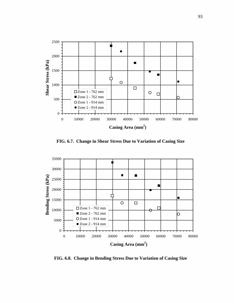
93

0

500

1000

1500

2000

2500

0 10000 20000 30000 40000 50000 60000 70000 80000

Casing Area (mm2)

Shea

r St

ress

(kPa

)


FIG. 6.7. Change in Shear Stress Due to Variation of Casing Size

0

5000

10000

15000

20000

25000

30000

35000

0 10000 20000 30000 40000 50000 60000 70000 80000

Casing Area (mm2)

Ben

ding

Str

ess (

kPa)


FIG. 6.8. Change in Bending Stress Due to Variation of Casing Size

94

6.2.4. Variation of Mudline Strength and Strength Gradient of the Soil

The effects of varying the mudline strength of the soil and the strength gradient of the soil

along the length of the casing below the mudline were studied. The mudline strength and

strength gradient values were varied ±10 percent and ±20 percent relative to the baseline

model values. The results are presented in Tables 6.6 to 6.9 and Figs. 6.9 to 6.16.

As the mudline strength increases, the period of the structure decreases approximately

four percent for the Zone 1 PGA and five percent for the Zone 2 PGA. Similarly,

increasing the strength gradient values from 0.38 kPa/m (D1/D1) up to 0.57 kPa/m

(D4/D4) resulted in a nearly linear decrease of approximately six percent in the model

period. Increasing the value of either parameter caused small decreases in the deflection

values obtained for the range of mudline strength and strength gradient values examined.

The shear stresses of acting on the piles increased between five and seven percent over

the range of values examined in this study. The bending stress and displacement values

for both parameters do not show a definitive pattern corresponding with the variation

values. This may be caused by the change in the length of the moment arm as the

strength gradient and mudline strength are varied, so that even as the shear forces

increase, the maximum bending moments could decrease or increase, depending on the

length of the moment arm. The SSR and CSR values for both parameters were less than

0.7 and were relatively unaffected by the changes in the mudline strength and the strength

gradient of the soil.

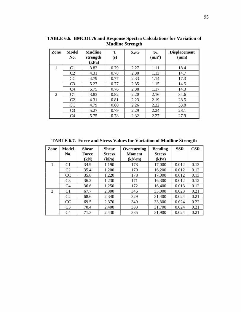
95

TABLE 6.6. BMCOL76 and Response Spectra Calculations for Variation of Mudline Strength

Zone Model No.

Mudline strength (kPa)

T (s)

SA/G SA (m/s2)

Displacement (mm)

C1 3.83 0.79 2.27 1.11 18.4 C2 4.31 0.78 2.30 1.13 14.7 CC 4.79 0.77 2.33 1.14 17.3 C3 5.27 0.77 2.35 1.15 14.5

1

C4 5.75 0.76 2.38 1.17 14.3 C1 3.83 0.82 2.20 2.16 34.6 C2 4.31 0.81 2.23 2.19 28.5 CC 4.79 0.80 2.26 2.22 33.8 C3 5.27 0.79 2.29 2.24 28.1

2

C4 5.75 0.78 2.32 2.27 27.9

TABLE 6.7. Force and Stress Values for Variation of Mudline Strength

Zone Model No.

Shear Force (kN)

Shear Stress (kPa)



SSR CSR

C1 34.9 1,190 178 17,000 0.012 0.13 C2 35.4 1,200 170 16,200 0.012 0.12 CC 35.8 1,220 178 17,000 0.012 0.13 C3 36.2 1,230 171 16,300 0.012 0.12

1

C4 36.6 1,250 172 16,400 0.013 0.12 C1 67.7 2,300 346 33,000 0.023 0.21 C2 68.6 2,340 329 31,400 0.024 0.21 CC 69.5 2,370 349 33,300 0.024 0.22 C3 70.4 2,400 333 31,700 0.024 0.21

2

C4 71.3 2,430 335 31,900 0.024 0.21

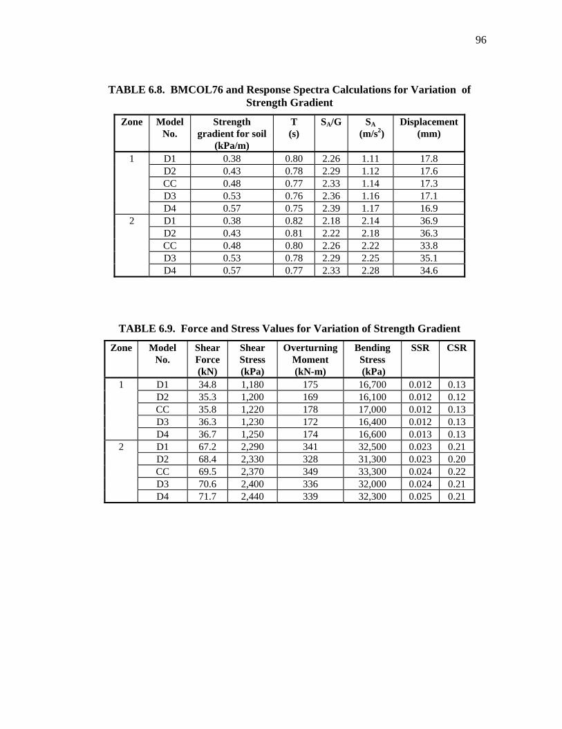
96

TABLE 6.8. BMCOL76 and Response Spectra Calculations for Variation of Strength Gradient

Zone Model No.

Strength gradient for soil

(kPa/m)

T (s)

SA/G SA (m/s2)

Displacement (mm)

D1 0.38 0.80 2.26 1.11 17.8 D2 0.43 0.78 2.29 1.12 17.6 CC 0.48 0.77 2.33 1.14 17.3 D3 0.53 0.76 2.36 1.16 17.1

1

D4 0.57 0.75 2.39 1.17 16.9 D1 0.38 0.82 2.18 2.14 36.9 D2 0.43 0.81 2.22 2.18 36.3 CC 0.48 0.80 2.26 2.22 33.8 D3 0.53 0.78 2.29 2.25 35.1

2

D4 0.57 0.77 2.33 2.28 34.6

TABLE 6.9. Force and Stress Values for Variation of Strength Gradient

Zone Model No.

Shear Force (kN)

Shear Stress (kPa)



SSR CSR

D1 34.8 1,180 175 16,700 0.012 0.13 D2 35.3 1,200 169 16,100 0.012 0.12 CC 35.8 1,220 178 17,000 0.012 0.13 D3 36.3 1,230 172 16,400 0.012 0.13

1

D4 36.7 1,250 174 16,600 0.013 0.13 D1 67.2 2,290 341 32,500 0.023 0.21 D2 68.4 2,330 328 31,300 0.023 0.20 CC 69.5 2,370 349 33,300 0.024 0.22 D3 70.6 2,400 336 32,000 0.024 0.21

2

D4 71.7 2,440 339 32,300 0.025 0.21

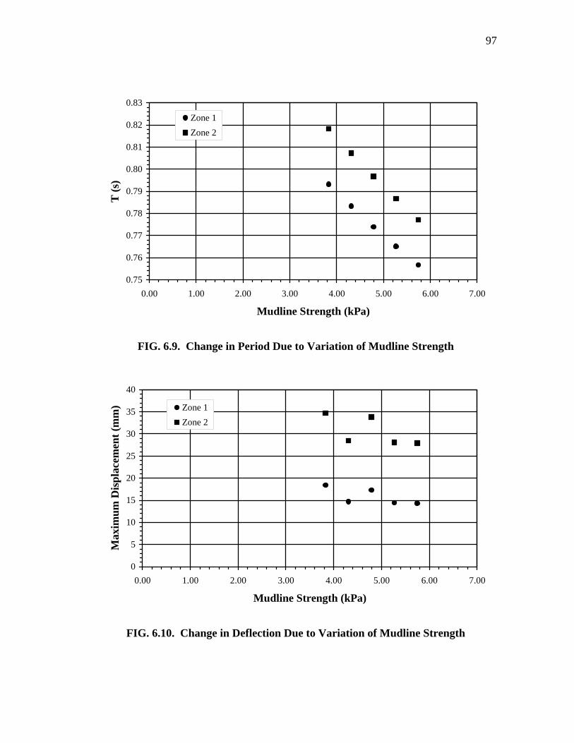
97

0.75

0.76

0.77

0.78

0.79

0.80

0.81

0.82

0.83

0.00 1.00 2.00 3.00 4.00 5.00 6.00 7.00

Mudline Strength (kPa)

T (s

)Zone 1Zone 2

FIG. 6.9. Change in Period Due to Variation of Mudline Strength

0

5

10

15

20

25

30

35

40

0.00 1.00 2.00 3.00 4.00 5.00 6.00 7.00


Max

imum

Dis

plac

emen

t (m

m) Zone 1

Zone 2

FIG. 6.10. Change in Deflection Due to Variation of Mudline Strength

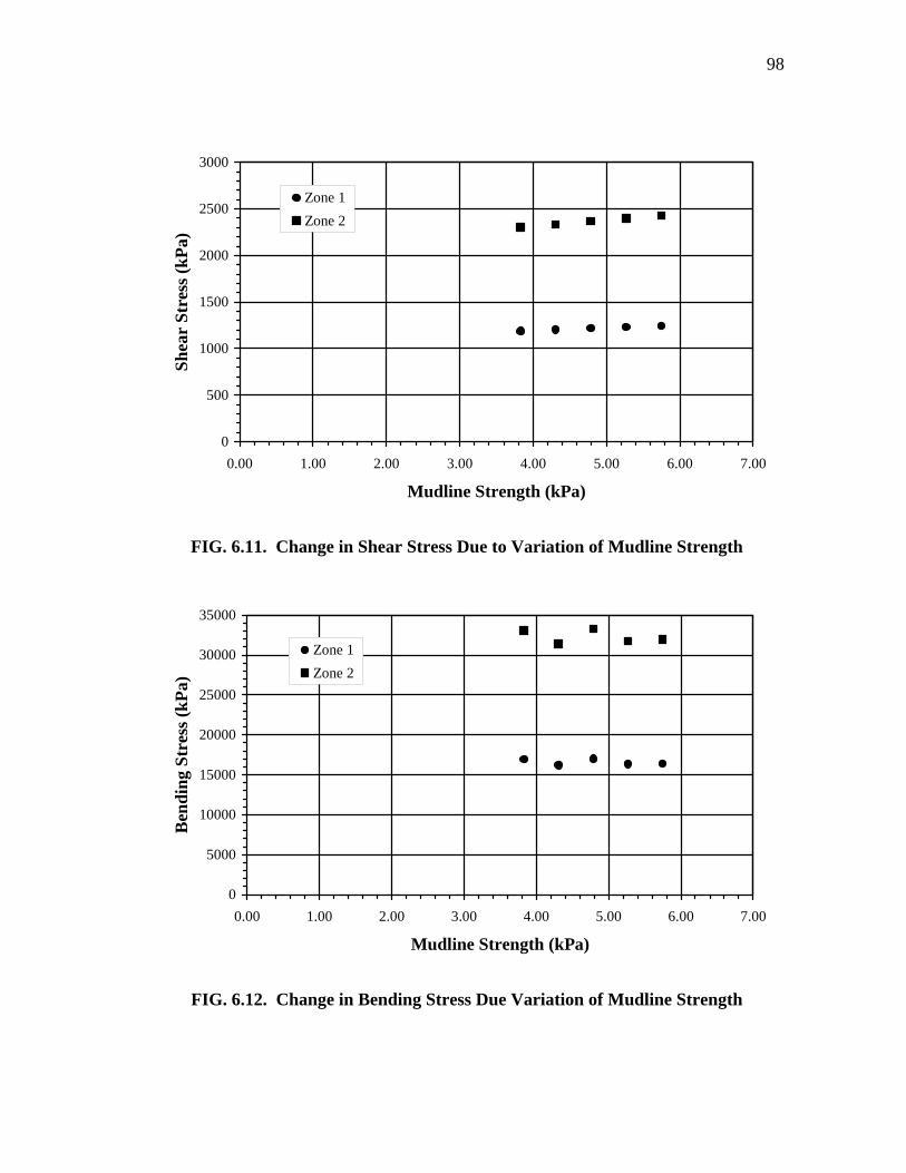
98

0

500

1000

1500

2000

2500

3000

0.00 1.00 2.00 3.00 4.00 5.00 6.00 7.00


Shea

r St

ress

(kPa

)Zone 1Zone 2

FIG. 6.11. Change in Shear Stress Due to Variation of Mudline Strength

0

5000

10000

15000

20000

25000

30000

35000

0.00 1.00 2.00 3.00 4.00 5.00 6.00 7.00


Ben

ding

Str

ess (

kPa)

Zone 1Zone 2

FIG. 6.12. Change in Bending Stress Due Variation of Mudline Strength

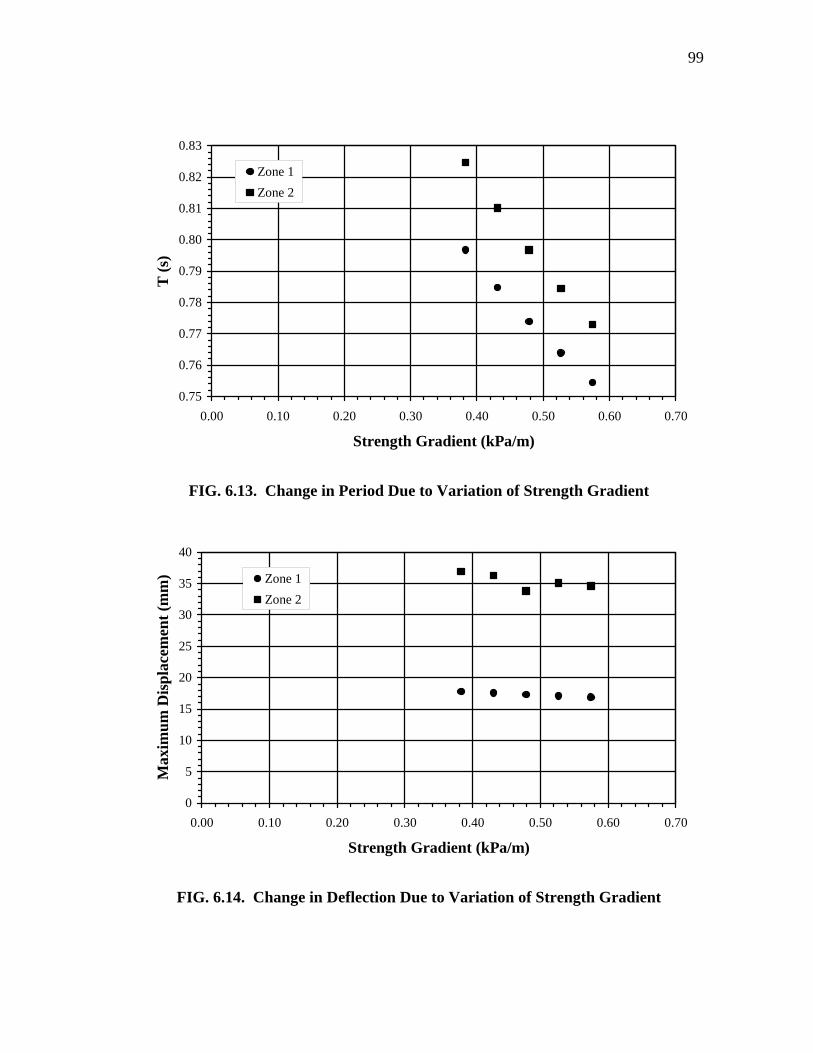
99

0.75

0.76

0.77

0.78

0.79

0.80

0.81

0.82

0.83

0.00 0.10 0.20 0.30 0.40 0.50 0.60 0.70

Strength Gradient (kPa/m)

T (s

)Zone 1Zone 2

FIG. 6.13. Change in Period Due to Variation of Strength Gradient

0

5

10

15

20

25

30

35

40

0.00 0.10 0.20 0.30 0.40 0.50 0.60 0.70


Max

imum

Dis

plac

emen

t (m

m) Zone 1

Zone 2

FIG. 6.14. Change in Deflection Due to Variation of Strength Gradient

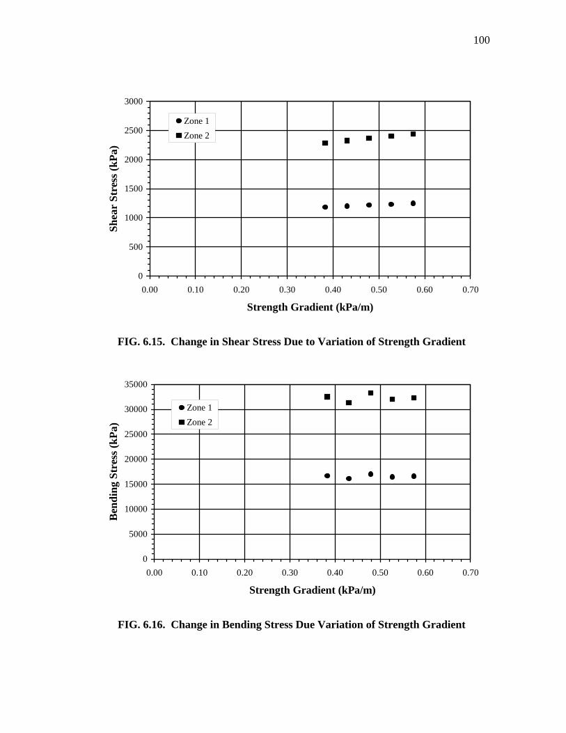
100

0

500

1000

1500

2000

2500

3000

0.00 0.10 0.20 0.30 0.40 0.50 0.60 0.70


Shea

r St

ress

(kPa

)Zone 1Zone 2

FIG. 6.15. Change in Shear Stress Due to Variation of Strength Gradient

0

5000

10000

15000

20000

25000

30000

35000

0.00 0.10 0.20 0.30 0.40 0.50 0.60 0.70


Ben

ding

Str

ess (

kPa)

Zone 1Zone 2

FIG. 6.16. Change in Bending Stress Due Variation of Strength Gradient

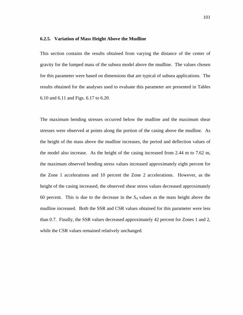
101

6.2.5. Variation of Mass Height Above the Mudline

This section contains the results obtained from varying the distance of the center of

gravity for the lumped mass of the subsea model above the mudline. The values chosen

for this parameter were based on dimensions that are typical of subsea applications. The

results obtained for the analyses used to evaluate this parameter are presented in Tables

6.10 and 6.11 and Figs. 6.17 to 6.20.

The maximum bending stresses occurred below the mudline and the maximum shear

stresses were observed at points along the portion of the casing above the mudline. As

the height of the mass above the mudline increases, the period and deflection values of

the model also increase. As the height of the casing increased from 2.44 m to 7.62 m,

the maximum observed bending stress values increased approximately eight percent for

the Zone 1 accelerations and 10 percent the Zone 2 accelerations. However, as the

height of the casing increased, the observed shear stress values decreased approximately

60 percent. This is due to the decrease in the SA values as the mass height above the

mudline increased. Both the SSR and CSR values obtained for this parameter were less

than 0.7. Finally, the SSR values decreased approximately 42 percent for Zones 1 and 2,

while the CSR values remained relatively unchanged.

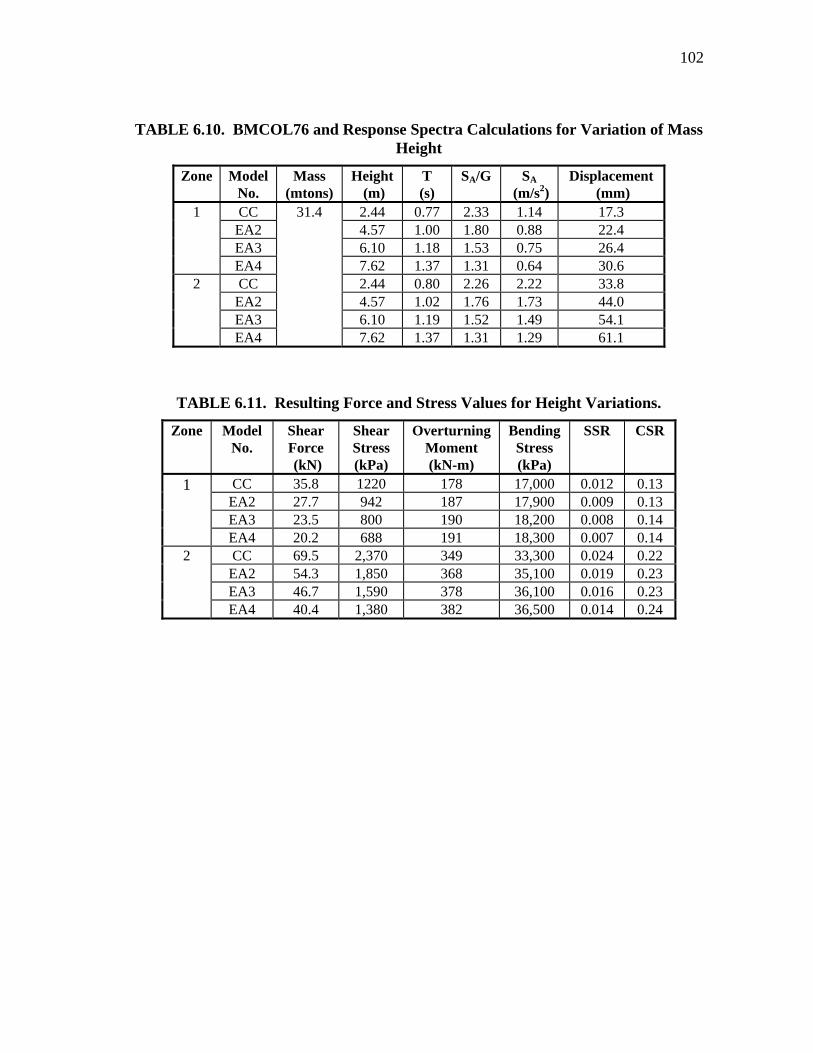
102

TABLE 6.10. BMCOL76 and Response Spectra Calculations for Variation of Mass Height

Zone Model No.

Mass (mtons)

Height (m)

T (s)

SA/G SA (m/s2)

Displacement (mm)

CC 2.44 0.77 2.33 1.14 17.3 EA2 4.57 1.00 1.80 0.88 22.4 EA3 6.10 1.18 1.53 0.75 26.4

1

EA4 7.62 1.37 1.31 0.64 30.6 CC 2.44 0.80 2.26 2.22 33.8

EA2 4.57 1.02 1.76 1.73 44.0 EA3 6.10 1.19 1.52 1.49 54.1

2

EA4

31.4

7.62 1.37 1.31 1.29 61.1

TABLE 6.11. Resulting Force and Stress Values for Height Variations.

Zone Model No.

Shear Force (kN)

Shear Stress (kPa)



SSR CSR

CC 35.8 1220 178 17,000 0.012 0.13 EA2 27.7 942 187 17,900 0.009 0.13 EA3 23.5 800 190 18,200 0.008 0.14

1

EA4 20.2 688 191 18,300 0.007 0.14 CC 69.5 2,370 349 33,300 0.024 0.22

EA2 54.3 1,850 368 35,100 0.019 0.23 EA3 46.7 1,590 378 36,100 0.016 0.23

2

EA4 40.4 1,380 382 36,500 0.014 0.24

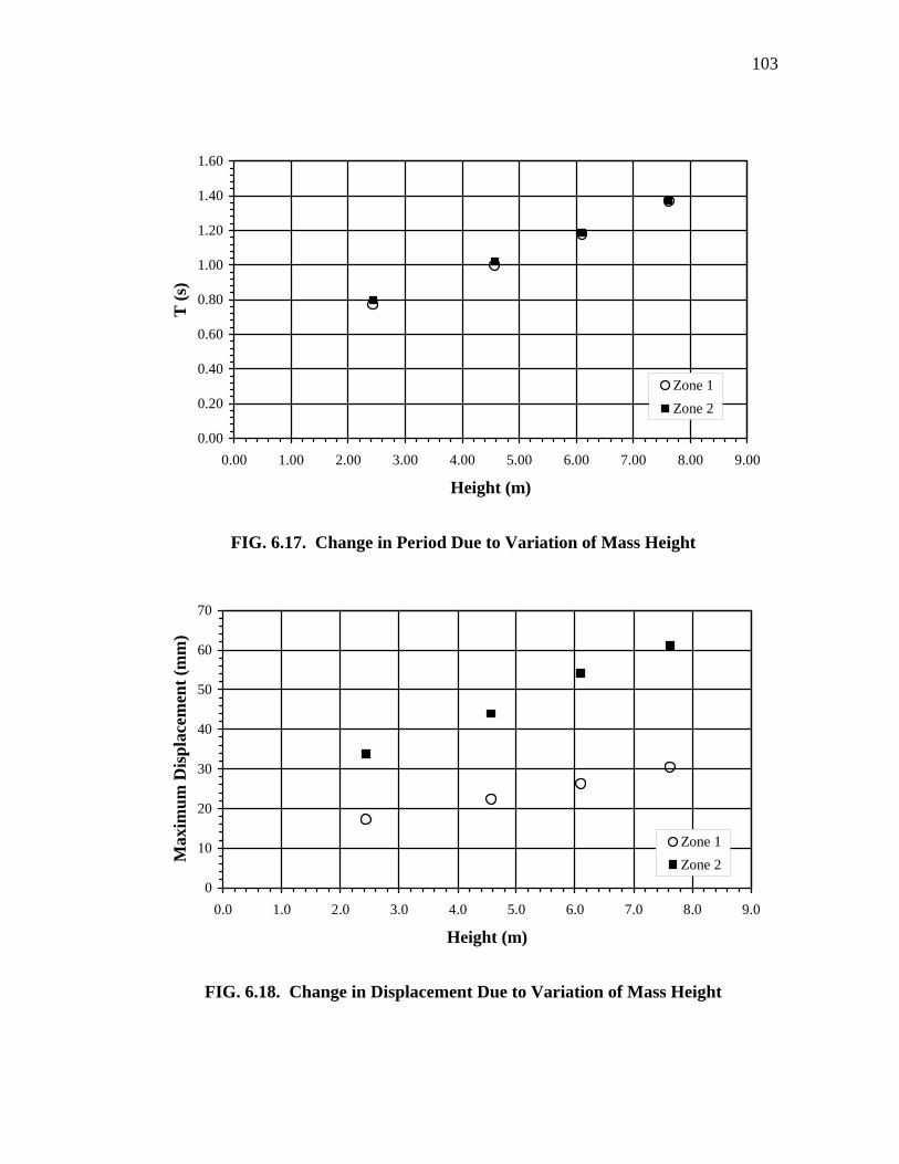
103

0.00

0.20

0.40

0.60

0.80

1.00

1.20

1.40

1.60

0.00 1.00 2.00 3.00 4.00 5.00 6.00 7.00 8.00 9.00

Height (m)

T (s

)

Zone 1Zone 2

FIG. 6.17. Change in Period Due to Variation of Mass Height

0

10

20

30

40

50

60

70

0.0 1.0 2.0 3.0 4.0 5.0 6.0 7.0 8.0 9.0

Height (m)

Max

imum

Dis

plac

emen

t (m

m)

Zone 1Zone 2

FIG. 6.18. Change in Displacement Due to Variation of Mass Height

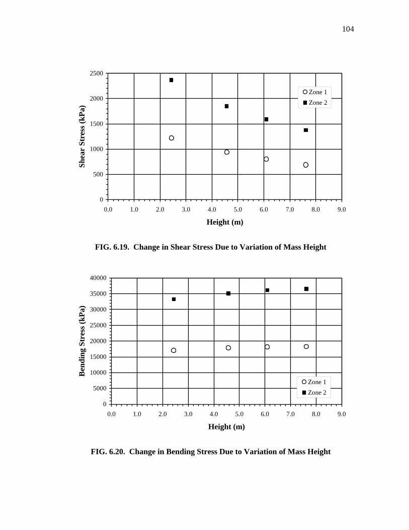
104

0

500

1000

1500

2000

2500

0.0 1.0 2.0 3.0 4.0 5.0 6.0 7.0 8.0 9.0

Height (m)

Shea

r St

ress

(kPa

)Zone 1Zone 2

FIG. 6.19. Change in Shear Stress Due to Variation of Mass Height

0

5000

10000

15000

20000

25000

30000

35000

40000

0.0 1.0 2.0 3.0 4.0 5.0 6.0 7.0 8.0 9.0

Height (m)

Ben

ding

Str

ess (

kPa)

Zone 1Zone 2

FIG. 6.20. Change in Bending Stress Due to Variation of Mass Height

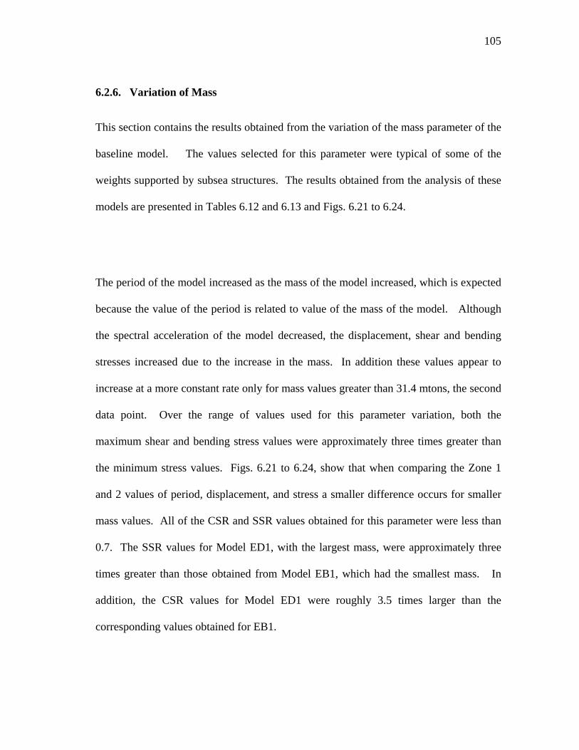
105

6.2.6. Variation of Mass

This section contains the results obtained from the variation of the mass parameter of the

baseline model. The values selected for this parameter were typical of some of the

weights supported by subsea structures. The results obtained from the analysis of these

models are presented in Tables 6.12 and 6.13 and Figs. 6.21 to 6.24.

The period of the model increased as the mass of the model increased, which is expected

because the value of the period is related to value of the mass of the model. Although

the spectral acceleration of the model decreased, the displacement, shear and bending

stresses increased due to the increase in the mass. In addition these values appear to

increase at a more constant rate only for mass values greater than 31.4 mtons, the second

data point. Over the range of values used for this parameter variation, both the

maximum shear and bending stress values were approximately three times greater than

the minimum stress values. Figs. 6.21 to 6.24, show that when comparing the Zone 1

and 2 values of period, displacement, and stress a smaller difference occurs for smaller

mass values. All of the CSR and SSR values obtained for this parameter were less than

0.7. The SSR values for Model ED1, with the largest mass, were approximately three

times greater than those obtained from Model EB1, which had the smallest mass. In

addition, the CSR values for Model ED1 were roughly 3.5 times larger than the

corresponding values obtained for EB1.

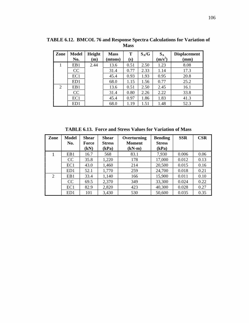
106

TABLE 6.12. BMCOL 76 and Response Spectra Calculations for Variation of Mass

Zone Model No.

Height (m)

Mass (mtons)

T (s)

SA/G SA (m/s2)

Displacement (mm)

EB1 13.6 0.51 2.50 1.23 8.08 CC 31.4 0.77 2.33 1.14 17.3 EC1 45.4 0.93 1.93 0.95 20.8

1

ED1 68.0 1.15 1.56 0.77 25.2 EB1 13.6 0.51 2.50 2.45 16.1 CC 31.4 0.80 2.26 2.22 33.8 EC1 45.4 0.97 1.86 1.83 41.3

2

ED1

2.44

68.0 1.19 1.51 1.48 52.3

TABLE 6.13. Force and Stress Values for Variation of Mass

Zone Model No.

Shear Force (kN)

Shear Stress (kPa)



SSR CSR

EB1 16.7 568 83.1 7,930 0.006 0.06 CC 35.8 1,220 178 17,000 0.012 0.13 EC1 43.0 1,460 214 20,500 0.015 0.16

1

ED1 52.1 1,770 259 24,700 0.018 0.21 EB1 33.4 1,140 166 15,900 0.011 0.10 CC 69.5 2,370 349 33,300 0.024 0.22 EC1 82.9 2,820 423 40,300 0.028 0.27

2

ED1 101 3,430 530 50,600 0.035 0.35

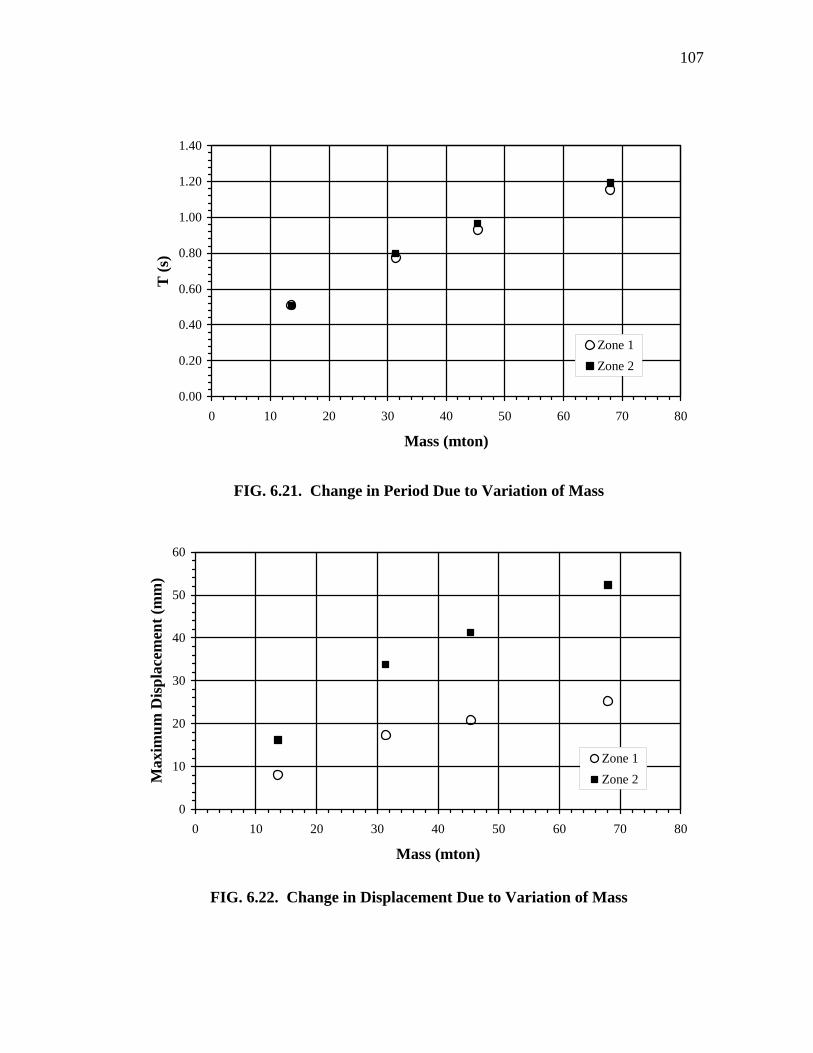
107

0.00

0.20

0.40

0.60

0.80

1.00

1.20

1.40

0 10 20 30 40 50 60 70 80

Mass (mton)

T (s

)

Zone 1Zone 2

FIG. 6.21. Change in Period Due to Variation of Mass

0

10

20

30

40

50

60

0 10 20 30 40 50 60 70 8

Mass (mton)

Max

imum

Dis

plac

emen

t (m

m)

0

Zone 1Zone 2

FIG. 6.22. Change in Displacement Due to Variation of Mass

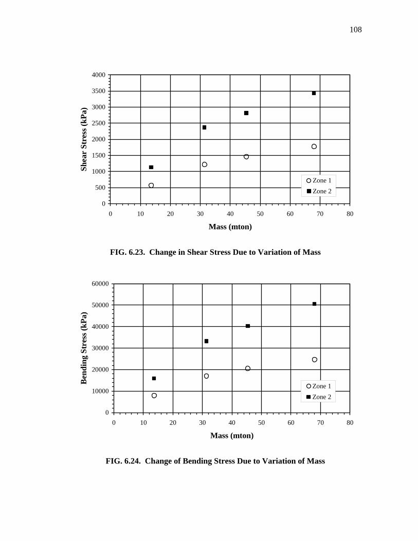
108

0

500

1000

1500

2000

2500

3000

3500

4000

0 10 20 30 40 50 60 70 80

Mass (mton)

Shea

r St

ress

(kPa

)

Zone 1Zone 2

FIG. 6.23. Change in Shear Stress Due to Variation of Mass

0

10000

20000

30000

40000

50000

60000

0 10 20 30 40 50 60 70 80

Mass (mton)

Ben

ding

Str

ess (

kPa)

Zone 1Zone 2

FIG. 6.24. Change of Bending Stress Due to Variation of Mass

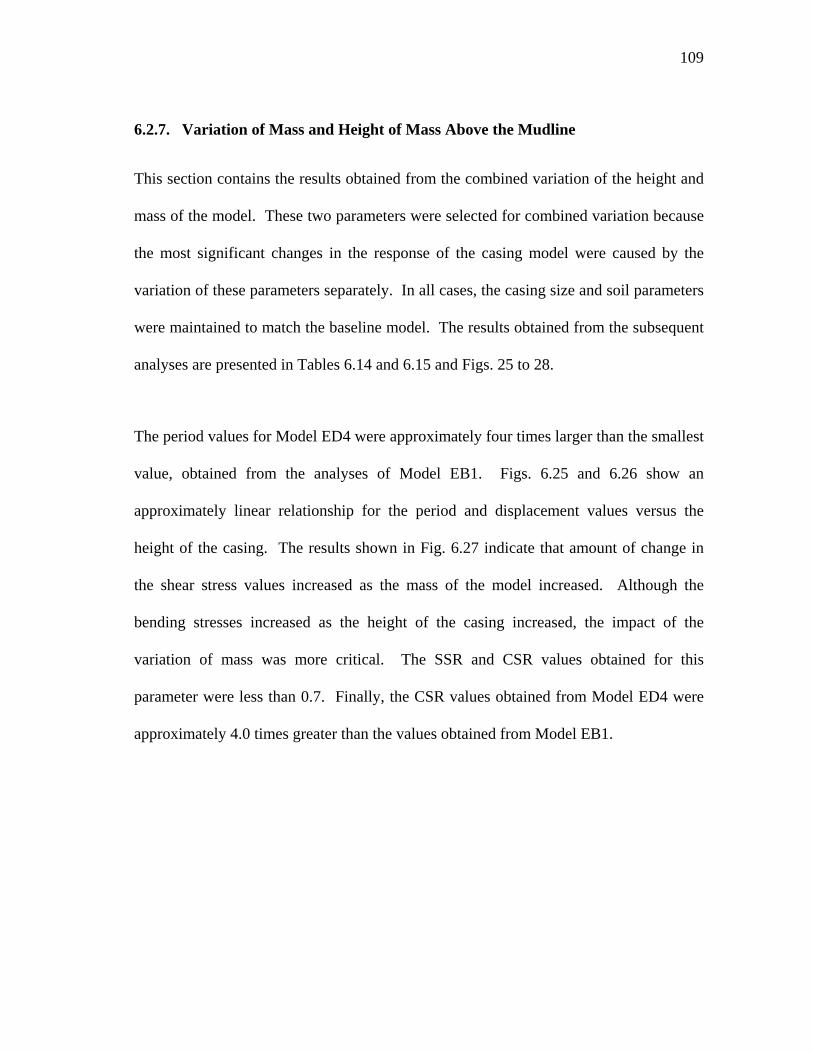
109

6.2.7. Variation of Mass and Height of Mass Above the Mudline

This section contains the results obtained from the combined variation of the height and

mass of the model. These two parameters were selected for combined variation because

the most significant changes in the response of the casing model were caused by the

variation of these parameters separately. In all cases, the casing size and soil parameters

were maintained to match the baseline model. The results obtained from the subsequent

analyses are presented in Tables 6.14 and 6.15 and Figs. 25 to 28.

The period values for Model ED4 were approximately four times larger than the smallest

value, obtained from the analyses of Model EB1. Figs. 6.25 and 6.26 show an

approximately linear relationship for the period and displacement values versus the

height of the casing. The results shown in Fig. 6.27 indicate that amount of change in

the shear stress values increased as the mass of the model increased. Although the

bending stresses increased as the height of the casing increased, the impact of the

variation of mass was more critical. The SSR and CSR values obtained for this

parameter were less than 0.7. Finally, the CSR values obtained from Model ED4 were

approximately 4.0 times greater than the values obtained from Model EB1.

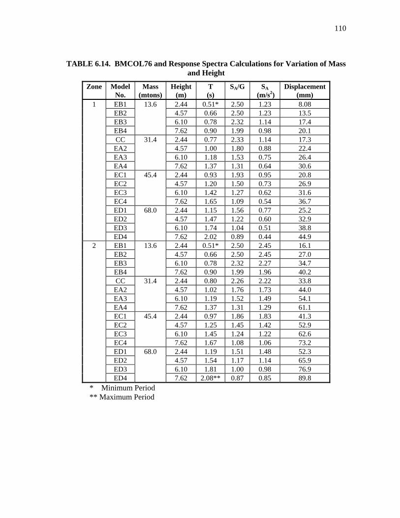
110

TABLE 6.14. BMCOL76 and Response Spectra Calculations for Variation of Mass and Height

Zone Model No.

Mass (mtons)

Height (m)

T (s)

SA/G SA (m/s2)

Displacement(mm)

EB1 2.44 0.51* 2.50 1.23 8.08 EB2 4.57 0.66 2.50 1.23 13.5 EB3 6.10 0.78 2.32 1.14 17.4 EB4

13.6

7.62 0.90 1.99 0.98 20.1 CC 2.44 0.77 2.33 1.14 17.3

EA2 4.57 1.00 1.80 0.88 22.4 EA3 6.10 1.18 1.53 0.75 26.4 EA4

31.4

7.62 1.37 1.31 0.64 30.6 EC1 2.44 0.93 1.93 0.95 20.8 EC2 4.57 1.20 1.50 0.73 26.9 EC3 6.10 1.42 1.27 0.62 31.6 EC4

45.4

7.62 1.65 1.09 0.54 36.7 ED1 2.44 1.15 1.56 0.77 25.2 ED2 4.57 1.47 1.22 0.60 32.9 ED3 6.10 1.74 1.04 0.51 38.8

1

ED4

68.0

7.62 2.02 0.89 0.44 44.9 EB1 2.44 0.51* 2.50 2.45 16.1 EB2 4.57 0.66 2.50 2.45 27.0 EB3 6.10 0.78 2.32 2.27 34.7 EB4

13.6

7.62 0.90 1.99 1.96 40.2 CC 2.44 0.80 2.26 2.22 33.8

EA2 4.57 1.02 1.76 1.73 44.0 EA3 6.10 1.19 1.52 1.49 54.1 EA4

31.4

7.62 1.37 1.31 1.29 61.1 EC1 2.44 0.97 1.86 1.83 41.3 EC2 4.57 1.25 1.45 1.42 52.9 EC3 6.10 1.45 1.24 1.22 62.6 EC4

45.4

7.62 1.67 1.08 1.06 73.2 ED1 2.44 1.19 1.51 1.48 52.3 ED2 4.57 1.54 1.17 1.14 65.9 ED3 6.10 1.81 1.00 0.98 76.9

2

ED4

68.0

7.62 2.08** 0.87 0.85 89.8 * Minimum Period ** Maximum Period

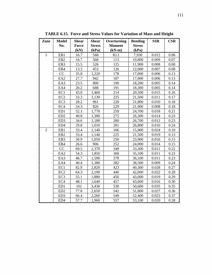
111

TABLE 6.15. Force and Stress Values for Variation of Mass and Height

Zone Model No.

Shear Force (kN)

Shear Stress (kPa)



SSR CSR

EB1 16.7 568 83.1 7,930 0.012 0.06 EB2 16.7 568 113 10,800 0.009 0.07 EB3 15.5 526 125 11,900 0.008 0.08 EB4 13.3 453 126 12,000 0.007 0.08 CC 35.8 1,220 178 17,000 0.006 0.13

EA2 27.7 942 187 17,900 0.006 0.13 EA3 23.5 800 190 18,200 0.005 0.14 EA4 20.2 688 191 18,300 0.005 0.14 EC1 43.0 1,460 214 20,500 0.015 0.16 EC2 33.3 1,130 225 21,500 0.011 0.17 EC3 28.2 961 228 21,800 0.010 0.18 EC4 24.3 826 229 21,900 0.008 0.18 ED1 52.1 1,770 259 24,700 0.018 0.21 ED2 40.8 1,390 275 26,300 0.014 0.23 ED3 34.6 1,180 280 26,700 0.012 0.23

1

ED4 29.8 1,010 281 26,800 0.010 0.24 EB1 33.4 1,140 166 15,900 0.024 0.10 EB2 33.4 1,140 225 21,500 0.019 0.13 EB3 30.9 1,050 250 23,900 0.016 0.15 EB4 26.6 906 252 24,000 0.014 0.15 CC 69.5 2,370 349 33,300 0.011 0.22

EA2 54.3 1,850 368 35,100 0.011 0.23 EA3 46.7 1,590 378 36,100 0.011 0.23 EA4 40.4 1,380 382 36,500 0.009 0.24 EC1 82.9 2,820 423 40,300 0.028 0.27 EC2 64.3 2,190 440 42,000 0.022 0.28 EC3 55.1 1,880 450 43,000 0.019 0.29 EC4 48.1 1,640 457 43,600 0.016 0.30 ED1 101 3,430 530 50,600 0.035 0.35 ED2 77.8 2,650 542 51,800 0.027 0.36 ED3 66.4 2,260 549 52,400 0.023 0.37

2

ED4 57.7 1,960 557 53,100 0.020 0.38

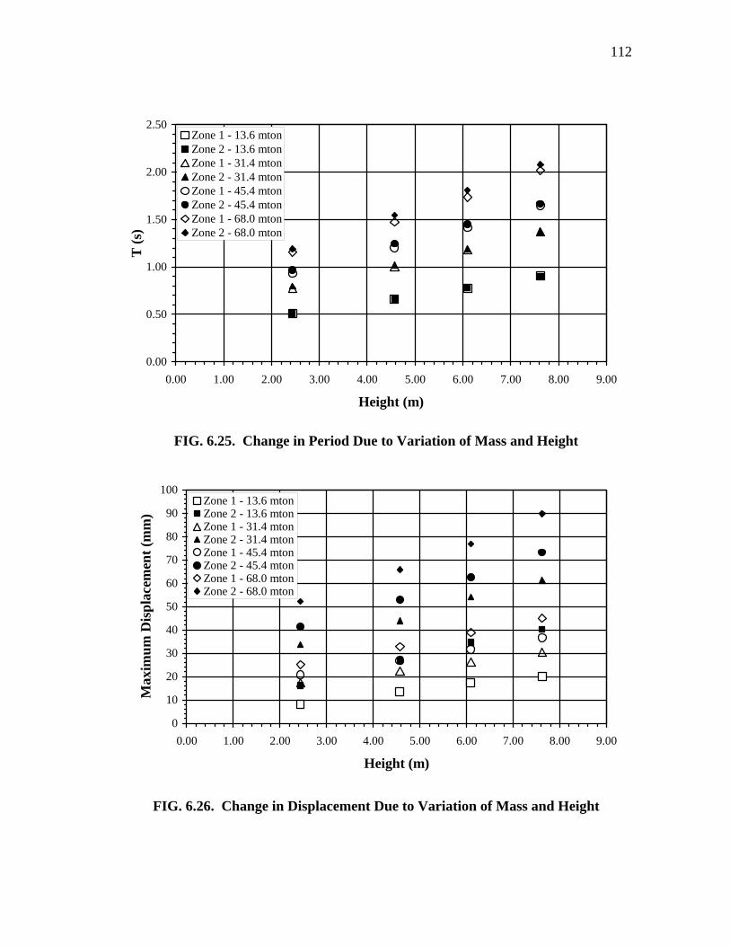
112

0.00

0.50

1.00

1.50

2.00

2.50

0.00 1.00 2.00 3.00 4.00 5.00 6.00 7.00 8.00 9.00

Height (m)

T (s

)Zone 1 - 13.6 mtonZone 2 - 13.6 mtonZone 1 - 31.4 mtonZone 2 - 31.4 mtonZone 1 - 45.4 mtonZone 2 - 45.4 mtonZone 1 - 68.0 mtonZone 2 - 68.0 mton

FIG. 6.25. Change in Period Due to Variation of Mass and Height

0

10

20

30

40

50

60

70

80

90

100

0.00 1.00 2.00 3.00 4.00 5.00 6.00 7.00 8.00 9.00

Height (m)

Max

imum

Dis

plac

emen

t (m

m)

Zone 1 - 13.6 mtonZone 2 - 13.6 mtonZone 1 - 31.4 mtonZone 2 - 31.4 mtonZone 1 - 45.4 mtonZone 2 - 45.4 mtonZone 1 - 68.0 mtonZone 2 - 68.0 mton

FIG. 6.26. Change in Displacement Due to Variation of Mass and Height

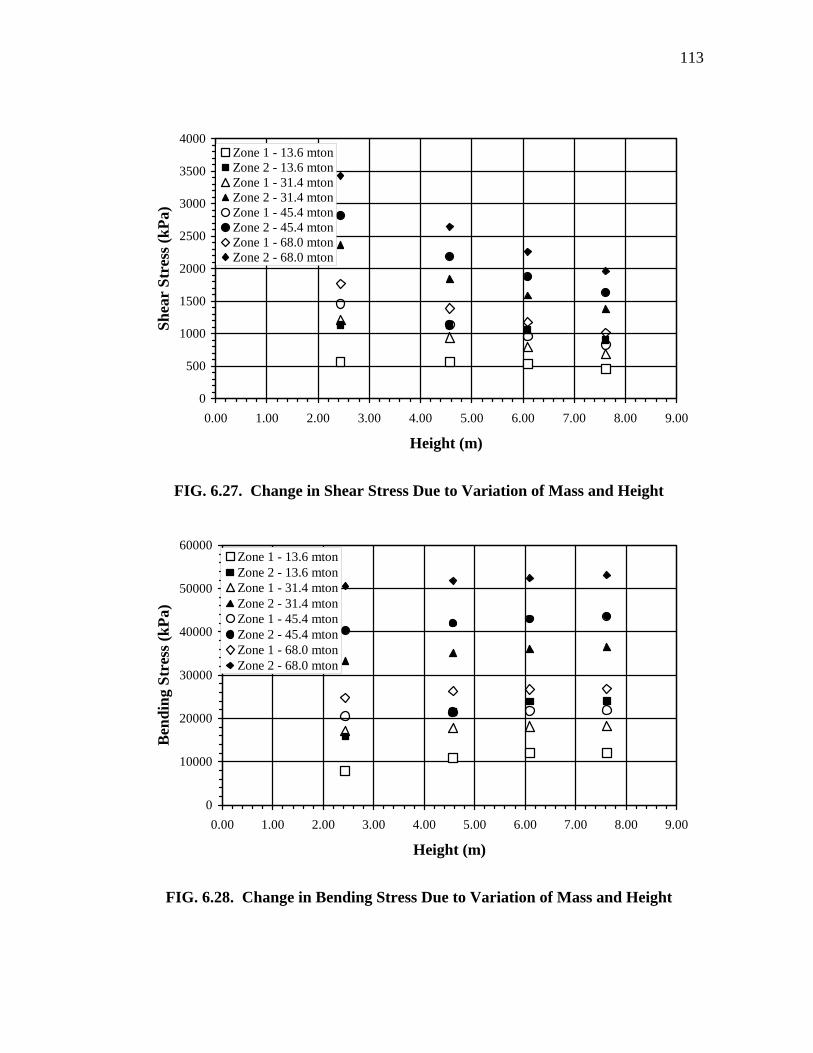
113

0

500

1000

1500

2000

2500

3000

3500

4000

0.00 1.00 2.00 3.00 4.00 5.00 6.00 7.00 8.00 9.00

Height (m)

Shea

r St

ress

(kPa

)Zone 1 - 13.6 mtonZone 2 - 13.6 mtonZone 1 - 31.4 mtonZone 2 - 31.4 mtonZone 1 - 45.4 mtonZone 2 - 45.4 mtonZone 1 - 68.0 mtonZone 2 - 68.0 mton

FIG. 6.27. Change in Shear Stress Due to Variation of Mass and Height

0

10000

20000

30000

40000

50000

60000

0.00 1.00 2.00 3.00 4.00 5.00 6.00 7.00 8.00 9.00

Height (m)

Ben

ding

Str

ess (

kPa)

Zone 1 - 13.6 mtonZone 2 - 13.6 mtonZone 1 - 31.4 mtonZone 2 - 31.4 mtonZone 1 - 45.4 mtonZone 2 - 45.4 mtonZone 1 - 68.0 mtonZone 2 - 68.0 mton

FIG. 6.28. Change in Bending Stress Due to Variation of Mass and Height

114

6.2.8. Fixity Variation

This section deals with the data generated by the analyses of the models with fixed-

headed casings. The top of the casings were fixed against rotation to simulate the lateral

resistance provided to an individual casing that is part of a multi-casing foundation.

Tables 6.16 and 6.17, along with Figs. 6.29 to 6.32, outline the results obtained from

these models. In addition, Figs. 6.29 to 6.32 include results from free-headed casing

models with comparable characteristics to the fixed-headed models.

Analysis of Model CCF yielded period values that were about half of the period values

obtained from the baseline model. Although the displacement of the model typically

increased as the height of the cantilever increased for the free-headed models, the

displacement values decreased as the height increased for the fixed-headed models. The

same behavior was observed in the range of bending stress values obtained for the fixed-

headed and free-headed models. However, the shear stresses from the fixed-headed

casings decreased as the height increased, although these values were significantly

higher than the stresses obtained from the comparable free-headed models. Although

the CSR and SSR values obtained are below the limiting ratio of 0.7. The SSR values

obtained from Model CCF were approximately ten percent higher than the ratios

obtained from the baseline model. The CSR values obtained from the fixed headed

models were approximately 1.4 to 1.8 times greater than the values obtained from the

corresponding free-headed models. The increase in these values is primarily due to the

increased bending stresses caused by fixing the casing against rotation.

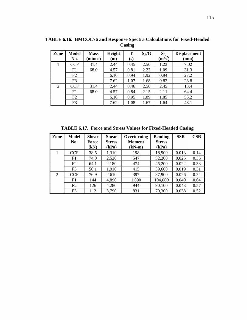
115

TABLE 6.16. BMCOL76 and Response Spectra Calculations for Fixed-Headed Casing

Zone Model No.

Mass (mtons)

Height (m)

T (s)

SA/G SA (m/s2)

Displacement(mm)

CCF 31.4 2.44 0.45 2.50 1.23 7.02 F1 4.57 0.81 2.22 1.09 31.3 F2 6.10 0.94 1.92 0.94 27.2

1

F3

68.0

7.62 1.07 1.68 0.82 23.8 CCF 31.4 2.44 0.46 2.50 2.45 13.4 F1 4.57 0.84 2.15 2.11 64.4 F2 6.10 0.95 1.89 1.85 55.2

2

F3

68.0

7.62 1.08 1.67 1.64 48.1

TABLE 6.17. Force and Stress Values for Fixed-Headed Casing

Zone Model No.

Shear Force (kN)

Shear Stress (kPa)



SSR CSR

CCF 38.5 1,310 198 18,900 0.013 0.14 F1 74.0 2,520 547 52,200 0.025 0.36 F2 64.1 2,180 474 45,200 0.022 0.33

1

F3 56.1 1,910 415 39,600 0.019 0.31 CCF 76.9 2,610 397 37,900 0.026 0.24 F1 144 4,890 1,090 104,000 0.049 0.64 F2 126 4,280 944 90,100 0.043 0.57

2

F3 112 3,790 831 79,300 0.038 0.52

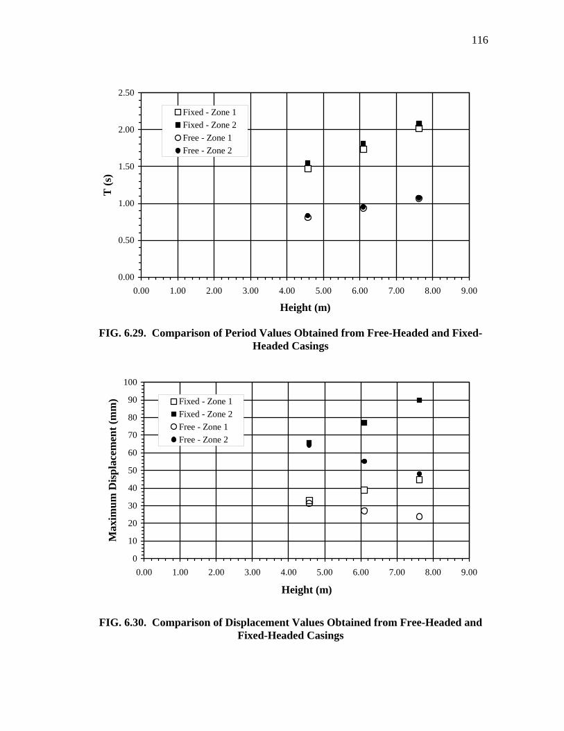
116

0.00

0.50

1.00

1.50

2.00

2.50

0.00 1.00 2.00 3.00 4.00 5.00 6.00 7.00 8.00 9.00

Height (m)

T (s

)Fixed - Zone 1Fixed - Zone 2Free - Zone 1Free - Zone 2

FIG. 6.29. Comparison of Period Values Obtained from Free-Headed and Fixed-

Headed Casings

0

10

20

30

40

50

60

70

80

90

100

0.00 1.00 2.00 3.00 4.00 5.00 6.00 7.00 8.00 9.00

Height (m)

Max

imum

Dis

plac

emen

t (m

m) Fixed - Zone 1

Fixed - Zone 2Free - Zone 1Free - Zone 2

FIG. 6.30. Comparison of Displacement Values Obtained from Free-Headed and

Fixed-Headed Casings

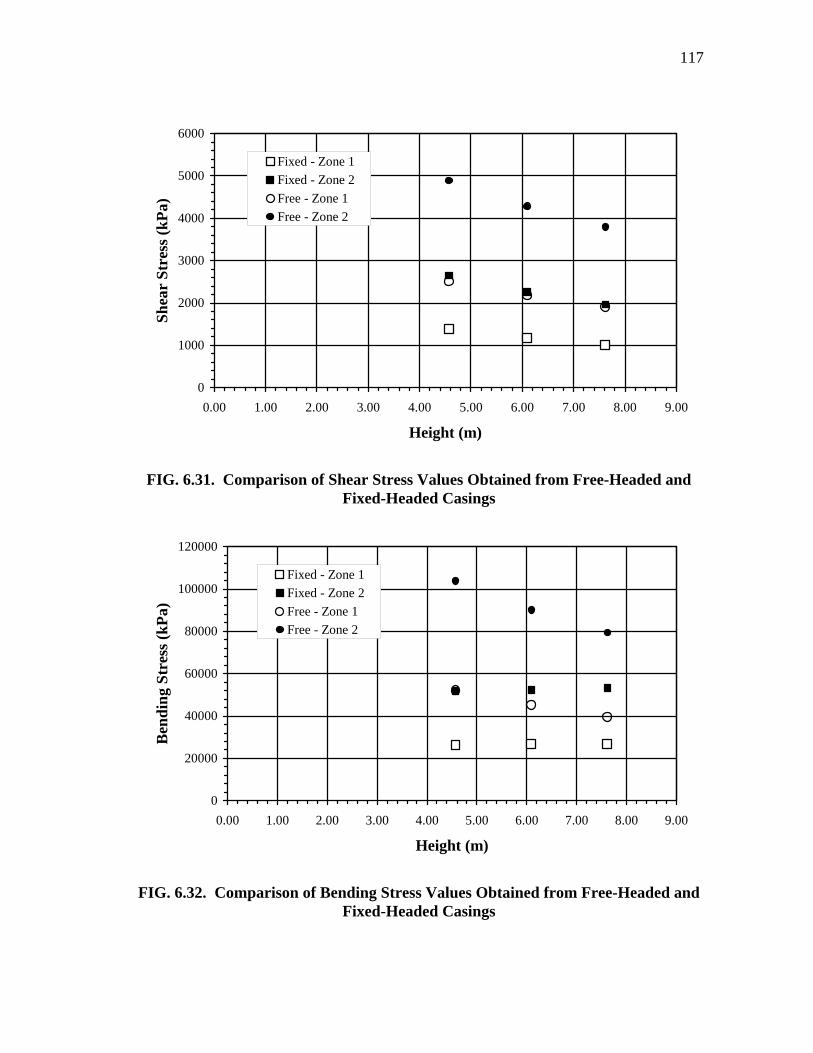
117

0

1000

2000

3000

4000

5000

6000

0.00 1.00 2.00 3.00 4.00 5.00 6.00 7.00 8.00 9.00

Height (m)

Shea

r St

ress

(kPa

)Fixed - Zone 1Fixed - Zone 2Free - Zone 1Free - Zone 2

FIG. 6.31. Comparison of Shear Stress Values Obtained from Free-Headed and


0

20000

40000

60000

80000

100000

120000

0.00 1.00 2.00 3.00 4.00 5.00 6.00 7.00 8.00 9.00

Height (m)

Ben

ding

Str

ess (

kPa)

Fixed - Zone 1Fixed - Zone 2Free - Zone 1Free - Zone 2

FIG. 6.32. Comparison of Bending Stress Values Obtained from Free-Headed and


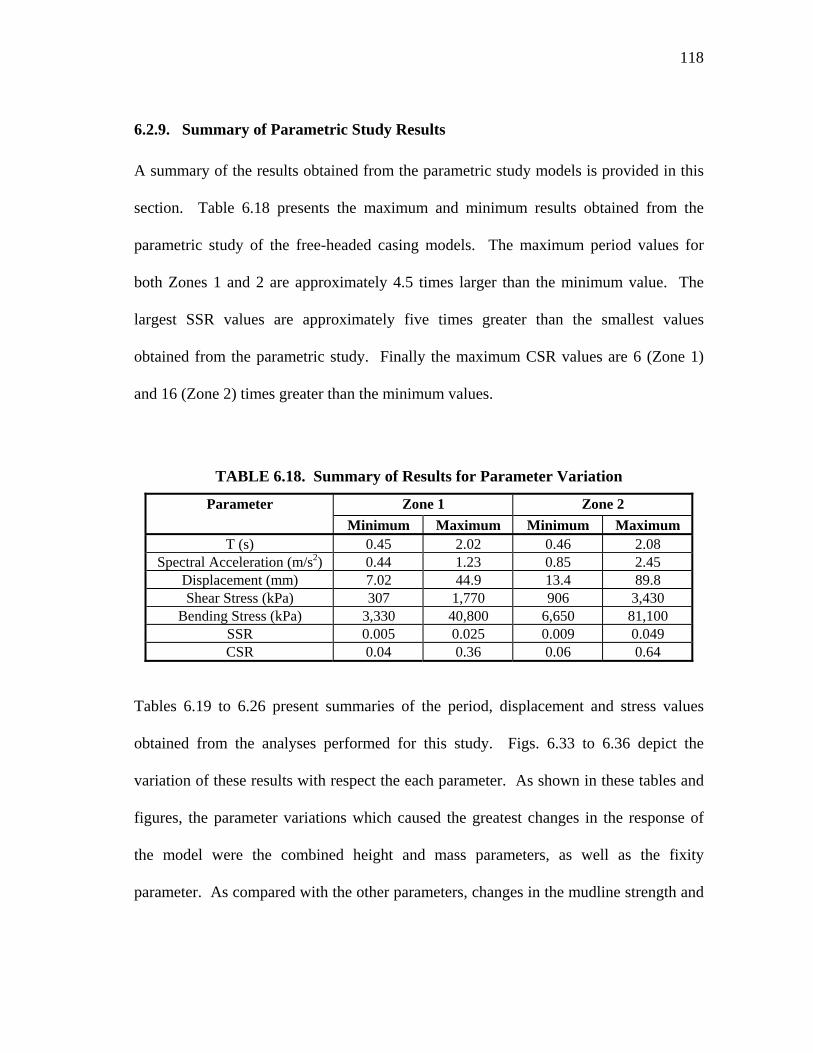
118

6.2.9. Summary of Parametric Study Results

A summary of the results obtained from the parametric study models is provided in this

section. Table 6.18 presents the maximum and minimum results obtained from the

parametric study of the free-headed casing models. The maximum period values for

both Zones 1 and 2 are approximately 4.5 times larger than the minimum value. The

largest SSR values are approximately five times greater than the smallest values

obtained from the parametric study. Finally the maximum CSR values are 6 (Zone 1)

and 16 (Zone 2) times greater than the minimum values.

TABLE 6.18. Summary of Results for Parameter Variation

Zone 1 Zone 2 Parameter Minimum Maximum Minimum Maximum

T (s) 0.45 2.02 0.46 2.08 Spectral Acceleration (m/s2) 0.44 1.23 0.85 2.45

Displacement (mm) 7.02 44.9 13.4 89.8 Shear Stress (kPa) 307 1,770 906 3,430

Bending Stress (kPa) 3,330 40,800 6,650 81,100 SSR 0.005 0.025 0.009 0.049 CSR 0.04 0.36 0.06 0.64

Tables 6.19 to 6.26 present summaries of the period, displacement and stress values

obtained from the analyses performed for this study. Figs. 6.33 to 6.36 depict the

variation of these results with respect the each parameter. As shown in these tables and

figures, the parameter variations which caused the greatest changes in the response of

the model were the combined height and mass parameters, as well as the fixity

parameter. As compared with the other parameters, changes in the mudline strength and

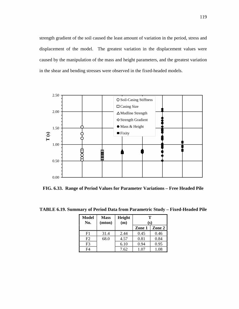
119

strength gradient of the soil caused the least amount of variation in the period, stress and

displacement of the model. The greatest variation in the displacement values were

caused by the manipulation of the mass and height parameters, and the greatest variation

in the shear and bending stresses were observed in the fixed-headed models.

0.00

0.50

1.00

1.50

2.00

2.50

T (s

)

Soil-Casing Stiffness

Casing Size

Mudline Strength

Strength Gradient

Mass & Height

Fixity

FIG. 6.33. Range of Period Values for Parameter Variations – Free Headed Pile

TABLE 6.19. Summary of Period Data from Parametric Study – Fixed-Headed Pile

T (s)

Model No.

Mass (mton)

Height (m)

Zone 1 Zone 2F1 31.4 2.44 0.45 0.46 F2 4.57 0.81 0.84 F3 6.10 0.94 0.95 F4

68.0

7.62 1.07 1.08

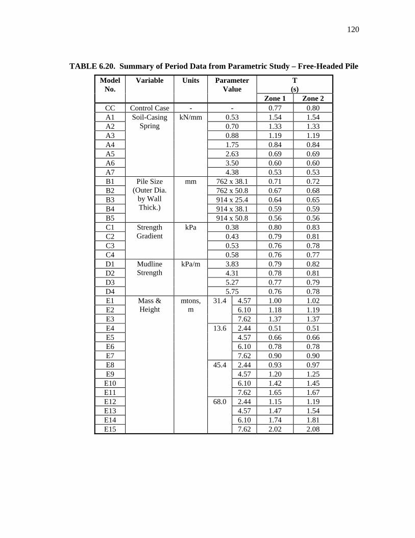
120

TABLE 6.20. Summary of Period Data from Parametric Study – Free-Headed Pile

T (s)

Model No.

Variable Units Parameter Value

Zone 1 Zone 2 CC Control Case - - 0.77 0.80 A1 0.53 1.54 1.54 A2 0.70 1.33 1.33 A3 0.88 1.19 1.19 A4 1.75 0.84 0.84 A5 2.63 0.69 0.69 A6 3.50 0.60 0.60 A7

Soil-Casing Spring

kN/mm

4.38 0.53 0.53 B1 762 x 38.1 0.71 0.72 B2 762 x 50.8 0.67 0.68 B3 914 x 25.4 0.64 0.65 B4 914 x 38.1 0.59 0.59 B5

Pile Size (Outer Dia.

by Wall Thick.)

mm

914 x 50.8 0.56 0.56 C1 0.38 0.80 0.83 C2 0.43 0.79 0.81 C3 0.53 0.76 0.78 C4

Strength Gradient

kPa

0.58 0.76 0.77 D1 3.83 0.79 0.82 D2 4.31 0.78 0.81 D3 5.27 0.77 0.79 D4

Mudline Strength

kPa/m

5.75 0.76 0.78 E1 4.57 1.00 1.02 E2 6.10 1.18 1.19 E3

31.4

7.62 1.37 1.37 E4 2.44 0.51 0.51 E5 4.57 0.66 0.66 E6 6.10 0.78 0.78 E7

13.6

7.62 0.90 0.90 E8 2.44 0.93 0.97 E9 4.57 1.20 1.25

E10 6.10 1.42 1.45 E11

45.4

7.62 1.65 1.67 E12 2.44 1.15 1.19 E13 4.57 1.47 1.54 E14 6.10 1.74 1.81 E15

Mass & Height

mtons, m

68.0

7.62 2.02 2.08

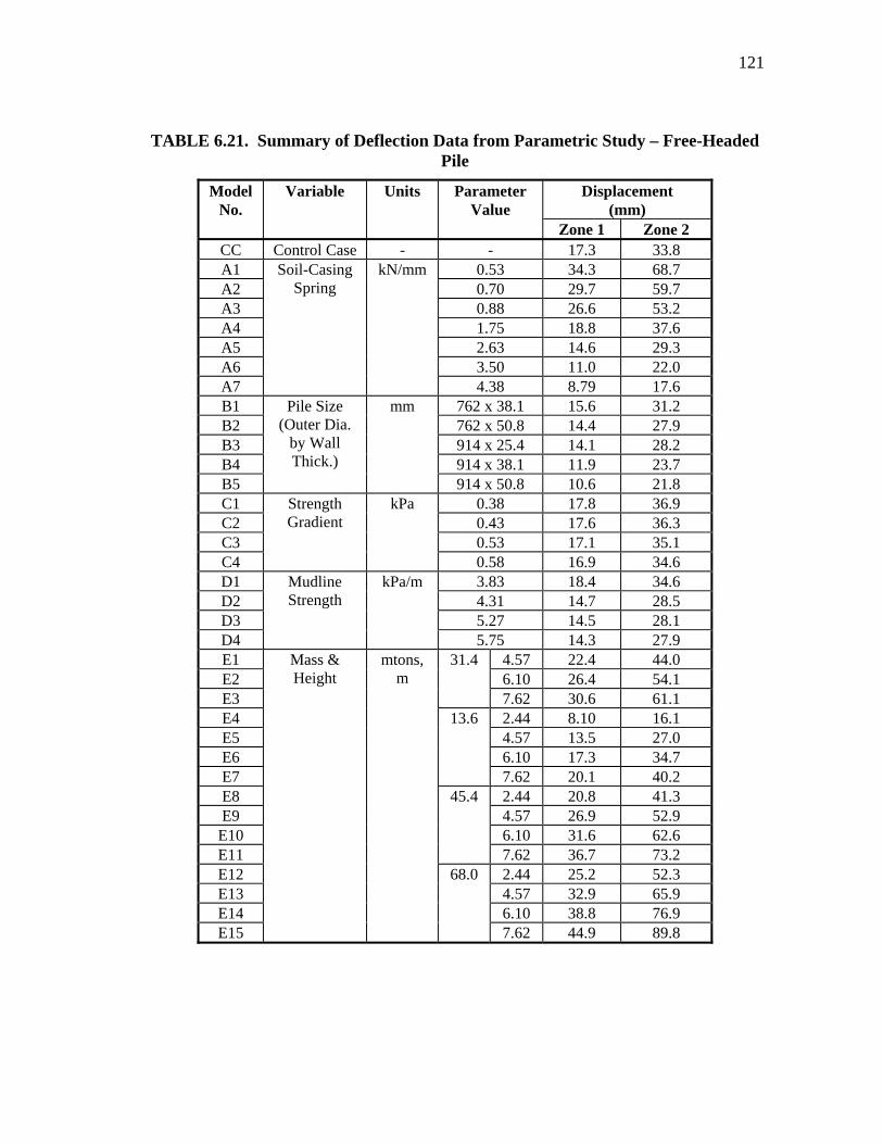
121

TABLE 6.21. Summary of Deflection Data from Parametric Study – Free-Headed Pile

Displacement (mm)

Model No.


Zone 1 Zone 2 CC Control Case - - 17.3 33.8 A1 0.53 34.3 68.7 A2 0.70 29.7 59.7 A3 0.88 26.6 53.2 A4 1.75 18.8 37.6 A5 2.63 14.6 29.3 A6 3.50 11.0 22.0 A7

Soil-Casing Spring

kN/mm

4.38 8.79 17.6 B1 762 x 38.1 15.6 31.2 B2 762 x 50.8 14.4 27.9 B3 914 x 25.4 14.1 28.2 B4 914 x 38.1 11.9 23.7 B5


by Wall Thick.)

mm

914 x 50.8 10.6 21.8 C1 0.38 17.8 36.9 C2 0.43 17.6 36.3 C3 0.53 17.1 35.1 C4

Strength Gradient

kPa

0.58 16.9 34.6 D1 3.83 18.4 34.6 D2 4.31 14.7 28.5 D3 5.27 14.5 28.1 D4

Mudline Strength

kPa/m

5.75 14.3 27.9 E1 4.57 22.4 44.0 E2 6.10 26.4 54.1 E3

31.4

7.62 30.6 61.1 E4 2.44 8.10 16.1 E5 4.57 13.5 27.0 E6 6.10 17.3 34.7 E7

13.6

7.62 20.1 40.2 E8 2.44 20.8 41.3 E9 4.57 26.9 52.9

E10 6.10 31.6 62.6 E11

45.4

7.62 36.7 73.2 E12 2.44 25.2 52.3 E13 4.57 32.9 65.9 E14 6.10 38.8 76.9 E15

Mass & Height

mtons, m

68.0

7.62 44.9 89.8

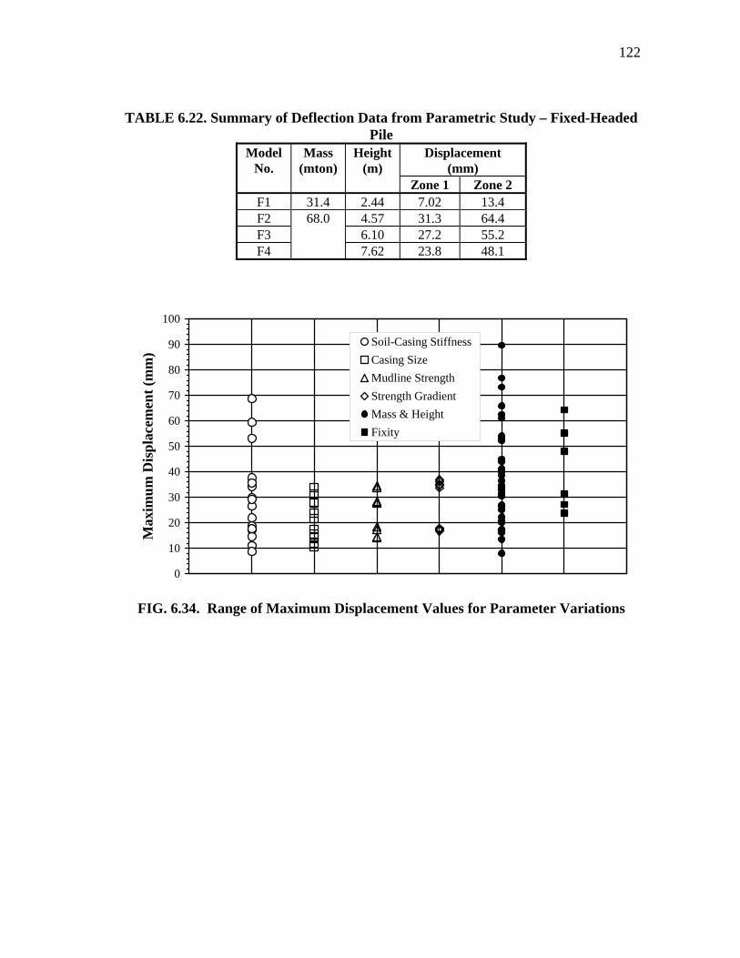
122

TABLE 6.22. Summary of Deflection Data from Parametric Study – Fixed-Headed Pile

Displacement (mm)

Model No.

Mass (mton)

Height (m)

Zone 1 Zone 2 F1 31.4 2.44 7.02 13.4 F2 4.57 31.3 64.4 F3 6.10 27.2 55.2 F4

68.0

7.62 23.8 48.1

0

10

20

30

40

50

60

70

80

90

100

Max

imum

Dis

plac

emen

t (m

m)

Soil-Casing StiffnessCasing SizeMudline StrengthStrength GradientMass & HeightFixity

FIG. 6.34. Range of Maximum Displacement Values for Parameter Variations

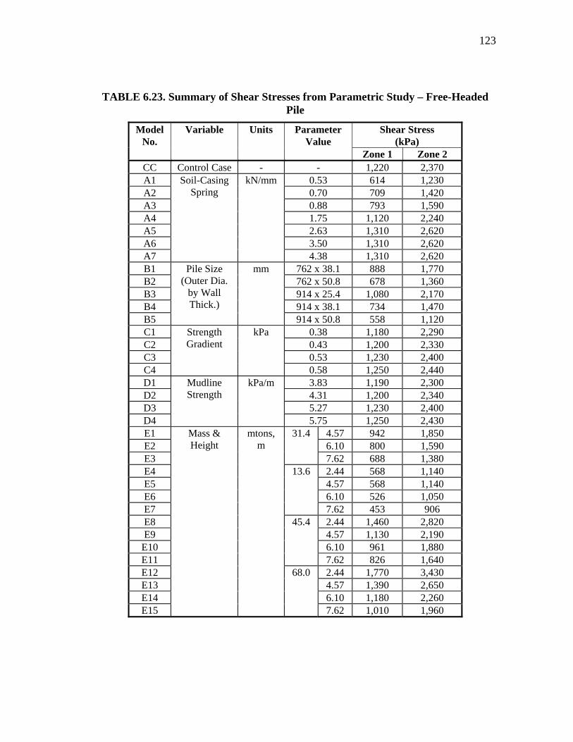
123

TABLE 6.23. Summary of Shear Stresses from Parametric Study – Free-Headed Pile

Shear Stress (kPa)

Model No.


Zone 1 Zone 2 CC Control Case - - 1,220 2,370 A1 0.53 614 1,230 A2 0.70 709 1,420 A3 0.88 793 1,590 A4 1.75 1,120 2,240 A5 2.63 1,310 2,620 A6 3.50 1,310 2,620 A7

Soil-Casing Spring

kN/mm

4.38 1,310 2,620 B1 762 x 38.1 888 1,770 B2 762 x 50.8 678 1,360 B3 914 x 25.4 1,080 2,170 B4 914 x 38.1 734 1,470 B5


by Wall Thick.)

mm

914 x 50.8 558 1,120 C1 0.38 1,180 2,290 C2 0.43 1,200 2,330 C3 0.53 1,230 2,400 C4

Strength Gradient

kPa

0.58 1,250 2,440 D1 3.83 1,190 2,300 D2 4.31 1,200 2,340 D3 5.27 1,230 2,400 D4

Mudline Strength

kPa/m

5.75 1,250 2,430 E1 4.57 942 1,850 E2 6.10 800 1,590 E3

31.4

7.62 688 1,380 E4 2.44 568 1,140 E5 4.57 568 1,140 E6 6.10 526 1,050 E7

13.6

7.62 453 906 E8 2.44 1,460 2,820 E9 4.57 1,130 2,190

E10 6.10 961 1,880 E11

45.4

7.62 826 1,640 E12 2.44 1,770 3,430 E13 4.57 1,390 2,650 E14 6.10 1,180 2,260 E15

Mass & Height

mtons, m

68.0

7.62 1,010 1,960

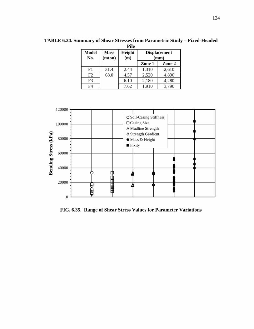
124

TABLE 6.24. Summary of Shear Stresses from Parametric Study – Fixed-Headed Pile

Displacement (mm)

Model No.

Mass (mton)

Height (m)

Zone 1 Zone 2 F1 31.4 2.44 1,310 2,610 F2 4.57 2,520 4,890 F3 6.10 2,180 4,280 F4

68.0

7.62 1,910 3,790

0

20000

40000

60000

80000

100000

120000

Ben

ding

Str

ess (

kPa)


FIG. 6.35. Range of Shear Stress Values for Parameter Variations

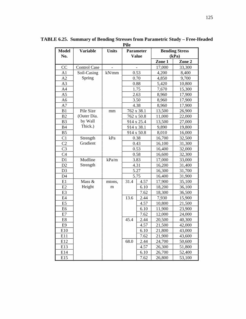
125

TABLE 6.25. Summary of Bending Stresses from Parametric Study – Free-Headed Pile


Model No.


Zone 1 Zone 2 CC Control Case - - 17,000 33,300 A1 0.53 4,200 8,400 A2 0.70 4,850 9,700 A3 0.88 5,420 10,800 A4 1.75 7,670 15,300 A5 2.63 8,960 17,900 A6 3.50 8,960 17,900 A7

Soil-Casing Spring

kN/mm

4.38 8,960 17,900 B1 762 x 38.1 13,500 26,900 B2 762 x 50.8 11,000 22,000 B3 914 x 25.4 13,500 27,000 B4 914 x 38.1 9,890 19,800 B5


by Wall Thick.)

mm

914 x 50.8 8,010 16,000 C1 0.38 16,700 32,500 C2 0.43 16,100 31,300 C3 0.53 16,400 32,000 C4

Strength Gradient

kPa

0.58 16,600 32,300 D1 3.83 17,000 33,000 D2 4.31 16,200 31,400 D3 5.27 16,300 31,700 D4

Mudline Strength

kPa/m

5.75 16,400 31,900 E1 4.57 17,900 35,100 E2 6.10 18,200 36,100 E3

31.4

7.62 18,300 36,500 E4 2.44 7,930 15,900 E5 4.57 10,800 21,500 E6 6.10 11,900 23,900 E7

13.6

7.62 12,000 24,000 E8 2.44 20,500 40,300 E9 4.57 21,500 42,000

E10 6.10 21,800 43,000 E11

45.4

7.62 21,900 43,600 E12 2.44 24,700 50,600 E13 4.57 26,300 51,800 E14 6.10 26,700 52,400 E15

Mass & Height

mtons, m

68.0

7.62 26,800 53,100

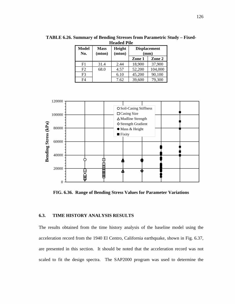
126

TABLE 6.26. Summary of Bending Stresses from Parametric Study – Fixed-Headed Pile

Displacement (mm)

Model No.

Mass (mton)

Height (mton)

Zone 1 Zone 2 F1 31.4 2.44 18,900 37,900 F2 4.57 52,200 104,000 F3 6.10 45,200 90,100 F4

68.0

7.62 39,600 79,300

0

20000

40000

60000

80000

100000

120000

Ben

ding

Str

ess (

kPa)


FIG. 6.36. Range of Bending Stress Values for Parameter Variations

6.3. TIME HISTORY ANALYSIS RESULTS

The results obtained from the time history analysis of the baseline model using the

acceleration record from the 1940 El Centro, California earthquake, shown in Fig. 6.37,

are presented in this section. It should be noted that the acceleration record was not

scaled to fit the design spectra. The SAP2000 program was used to determine the

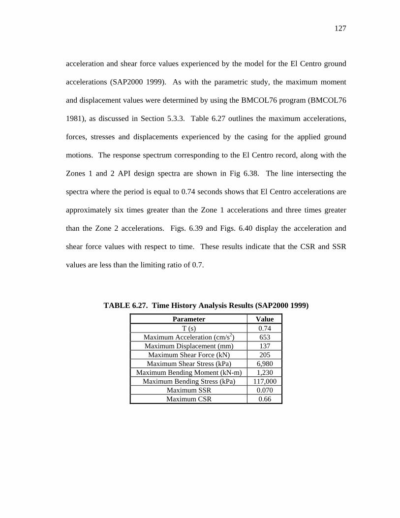
127

acceleration and shear force values experienced by the model for the El Centro ground

accelerations (SAP2000 1999). As with the parametric study, the maximum moment

and displacement values were determined by using the BMCOL76 program (BMCOL76

1981), as discussed in Section 5.3.3. Table 6.27 outlines the maximum accelerations,

forces, stresses and displacements experienced by the casing for the applied ground

motions. The response spectrum corresponding to the El Centro record, along with the

Zones 1 and 2 API design spectra are shown in Fig 6.38. The line intersecting the

spectra where the period is equal to 0.74 seconds shows that El Centro accelerations are

approximately six times greater than the Zone 1 accelerations and three times greater

than the Zone 2 accelerations. Figs. 6.39 and Figs. 6.40 display the acceleration and

shear force values with respect to time. These results indicate that the CSR and SSR

values are less than the limiting ratio of 0.7.

TABLE 6.27. Time History Analysis Results (SAP2000 1999)

Parameter Value T (s) 0.74

Maximum Acceleration (cm/s2) 653 Maximum Displacement (mm) 137 Maximum Shear Force (kN) 205 Maximum Shear Stress (kPa) 6,980

Maximum Bending Moment (kN-m) 1,230 Maximum Bending Stress (kPa) 117,000

Maximum SSR 0.070 Maximum CSR 0.66

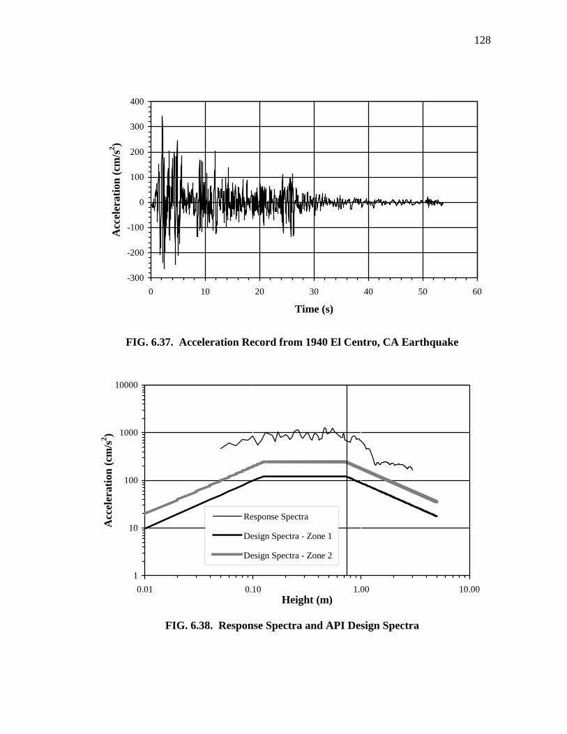
128

-300

-200

-100

0

100

200

300

400

0 10 20 30 40 50 6

Time (s)

Acc

eler

atio

n (c

m/s

2 )

0

FIG. 6.37. Acceleration Record from 1940 El Centro, CA Earthquake

1

10

100

1000

10000

0.01 0.10 1.00 10.00Height (m)

Acc

eler

atio

n (c

m/s2 )

Response Spectra

Design Spectra - Zone 1

Design Spectra - Zone 2

FIG. 6.38. Response Spectra and API Design Spectra

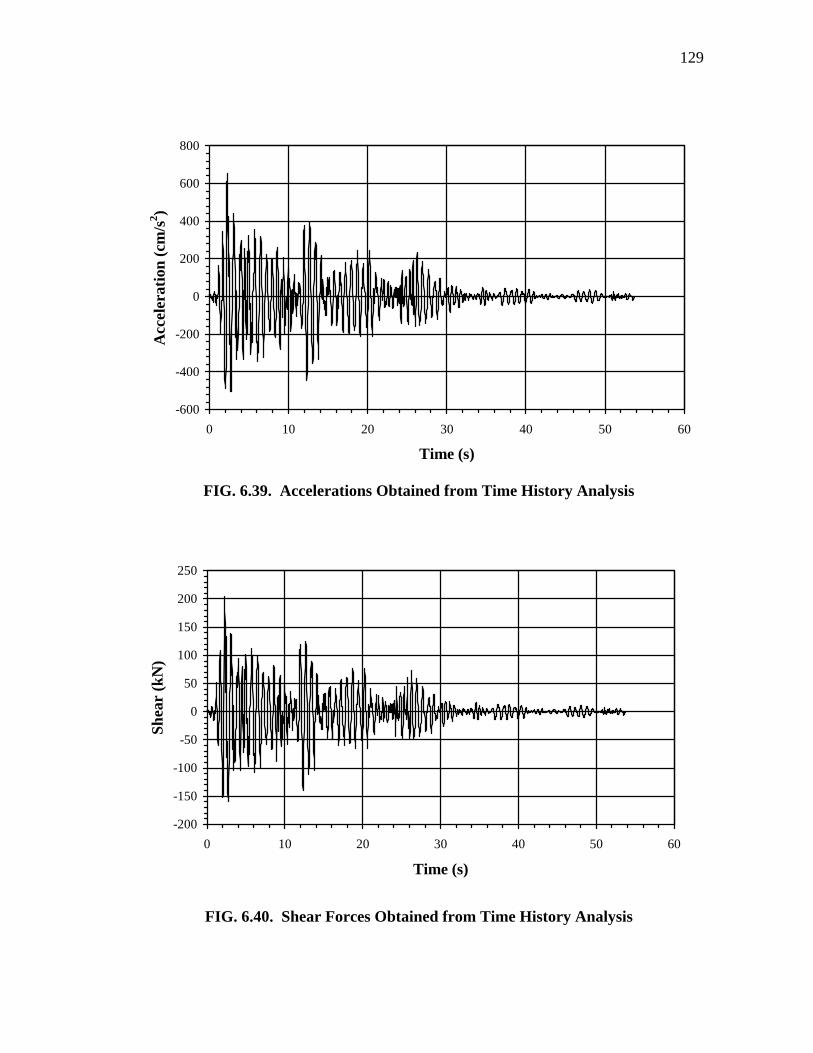
129

-600

-400

-200

0

200

400

600

800

0 10 20 30 40 50 6

Time (s)

Acc

eler

atio

n (c

m/s

2 )

0

FIG. 6.39. Accelerations Obtained from Time History Analysis

-200

-150

-100

-50

0

50

100

150

200

250

0 10 20 30 40 50 6

Time (s)

Shea

r (k

N)

0

FIG. 6.40. Shear Forces Obtained from Time History Analysis

130

6.4. CONCLUSION

The results from this study show that the height, mass, and fixity of the SDOF model

have the greatest effect on the response of the model to earthquake loading. In general,

increasing the mass and height of the model caused the stress and displacement values to

increase. Fixing the casing against rotation at the mass location caused the stress

values to increase. As the height of the casing increased, the bending stress decreased.

As expected, increasing the casing sizes caused the stresses and displacement values to

decrease. Variation of the mudline strength and strength gradient parameters, within the

ranges used in this study, did not cause significant changes in the stresses or

displacements.

The SSR values obtained from both the parametric study and time history analysis were

typically very small. The maximum CSR values obtained from the parametric study and

the time history analysis approach 0.7, however, these values never exceed this limit.

The stresses induced by Zones 1 and 2 accelerations are not substantial in comparison to

other possible lateral loads applied to subsea systems, such as riser loads. Finally, the

maximum displacement value obtained from the time history analysis is about 30

percent larger than the maximum value obtained from the parametric study.

Debbie Oakes

Note


Debbie Oakes

Note


Debbie Oakes

Note


131

7. SUMMARY AND CONCLUSIONS

7.1. SUMMARY

The number of deepwater subsea systems in the GOM continues to increase due to

technological advances and the ever increasing demand for energy. Since the GOM is

rather benign for earthquake potential, API does not require that offshore structures in

this region be designed for earthquakes. As a result, questions have been raised

regarding their seismic vulnerability. Earthquake shaking, liquefaction potential, and

soil sliding due to slope instability are three earthquake related factors that can impact

the performance of subsea structures. The focus of this research was to evaluate the

performance of these systems in deepwater environments in the GOM during potential

earthquake shaking.

The first task of this study was to review available information on the seismicity of the

GOM. As demonstrated by the seismic zone rating applied to this region, the seismic

risk in the GOM is considered to be low. However, a number of earthquakes have been

recorded in this region, most with Richter magnitude values greater than 3.0. The

largest recorded event, which occurred in the Mississippi Fan area, had a Richter

magnitude of 4.9. The second task of this research was to survey the range of systems

used in subsea applications. These structures included subsea wellheads, subsea

Christmas trees, templates and manifolds; all of which are supported by either single or

multiple casing foundations, depending on the application and design requirements. In

132

addition, a survey of the deepwater subsea systems located in the Gulf of Mexico was

conducted. Most of the systems included in this survey are located in the vicinity of the

grouping of earthquake epicenters in the Mississippi Fan area.

The models, parametric study, and analysis procedures were based on the information

gathered on subsea systems and earthquakes in the Gulf of Mexico. In addition, a

survey of the current practices for the structural design of offshore structures provided

critical information for the analyses. The prototype structure selected for this study was

a single wellhead subsea Christmas tree embedded in clay soils typical of the Gulf of

Mexico. The baseline analytical model was derived from the prototype structure, and

the parameters chosen for variation included the mass, height, base fixity, and soil

properties. The soil-casing stiffness, accelerations, and corresponding stresses were

determined using the BMCOL76 program and the response spectra method. In addition,

a time history analysis of the baseline analytical model was conducted using the ground

motion record obtained from the 1940 El Centro, California earthquake.

133

7.2. CONCLUSIONS

The following conclusions were made based on the results of the study.

1. A review of the information available on the GOM, classified by API RP2A as a Zone 0 seismic risk area,confirms that the seismicity of this area is relatively low.

2. Model subsea wells were analyzed with Zone 1 and Zone 2 seismic accelerations to provide a conservative bound for Zone 0 area such as the Gulf of Mexico. In general, the stresses produced by the simulated earthquake loads are relatively

negligible for the free-headed casing models in Zones 1 and 2 accelerations. As with

the free-headed casing models, most of stress ratio values observed for the fixed-

headed models were well within the allowable limits for the selected earthquake

loads. Maximum CSR values obtained from the parametric study approach, but

never exceed, the limiting ratio value of 0.7 for seismic loading. In addition, the

displacements induced in the analytical models by these loads also seem to be

within the range of values that could be reasonably expected to occur during the

course of normal operating conditions. These conditions include pipeline shifting and

movement caused from the tension in the attached risers.

3. The results from the parametric study indicate that the base fixity, mass, and height

parameters have the greatest effect on the response of the subsea structure to lateral

loading. Increasing the mass and height parameters of the free-headed casing

models, which simulate the responses of single casing structures, generally caused

Debbie Oakes

Note


Debbie Oakes

Note


Debbie Oakes

Note


Debbie Oakes

Note


134

the stress and displacements due to lateral loading to increase. Although the shear

and bending stresses obtained from the fixed-headed models were higher than those

obtained from the corresponding free-headed models, the stress values decreased as

the height of the casing increased above the mudline. The CSR values observed for

the fixed-headed models ranged between 0.14 and 0.64. The range of CSR values

obtained for the free-headed casing models was between 0.04 and 0.64.

4. The period, mass, height of the casing above the mudline, and base fixity dictate the

magnitude of stress and displacement values observed in the casing. When the mass,

height, and fixity remain unchanged; the stress and displacement values did not vary

for period values between 0.125 and 0.72 seconds. For periods between 0.0 and

0.125 seconds, the stress and displacement values increase. Finally, these values

decreased as the period increased above 0.72 seconds.

5. A time history analysis was completed to compare with the parametric analysis. The El Centro earthquake ground motion was used; ground accelerations are 6X those for API Zone 1 and 3X those for Zone 2. Even with these conservative ground motions, the results show that the maximum SSR value obtained from

the baseline free-headed casing model for the El Centro ground motion record

falls well below the limiting stress ratio for earthquake loads. It should be noted that

the maximum CSR value, 0.66, is close to the limiting ratio of 0.7. Although the

largest displacement value is greater than the values obtained from the parametric

study, this value should still fall within the range of allowable displacements for subsea structures.

Debbie Oakes

Note


Debbie Oakes

Note


Debbie Oakes

Note


Debbie Oakes

Note


Debbie Oakes

Note


Debbie Oakes

Note


135

7.3. RECOMMENDATIONS

1. The impact of earthquake shaking on the integrity of a single and multiple casing

foundation subsea structures is dependent upon a number of different factors that are

specific to site and system requirements. Seismic risk for proposed projects should

be investigated for specific site conditions and equipment constraints. Specific

design information for a subsea system is critical in making a final assessment of the

expected performance under site specific ground motions.

2. Based on the results from this study, earthquake shaking (within Zones 1 and 2 PGA

values) should not dramatically impact the performance of deepwater subsea

structures in the GOM. However, further research should be conducted to determine

the impact of sliding soil due to soil instability on the performance of these

structures in the GOM.

136

REFERENCES

American Petroleum Institute (API). (1996). “Recommended Practice for Design and

Operation of Subsea Production Systems.” API-RP17A, 2nd ed., Washington, D.C.

American Petroleum Institute (API). (2000a). “Recommended Practice for Planning,

Designing, and Constructing Fixed Offshore Platforms - Working Stress

Design.” API-RP2A, 21st ed., Washington D.C.

American Petroleum Institute (API). (2000b). “Recommended Practice for Planning,

Designing, and Constructing Fixed Offshore Platforms – Load and Resistance Factor

Design.” API-RP2A, 21st ed., Washington D.C.

BMCOL76 (1981). The Earth Technology Corporation, Long Beach, CA.

Bea, R.G. (1999). “Reliability Based Earthquake Design Guidelines for Marine Structures.”

J. of Waterway, Port, Coastal, and Ocean Engrg., ASCE, 125(5), 219 - 231.

Bednar, J.M. (1993). “The Zinc Subsea Production System: An Overview.” Proc. Offshore

Technol. Conf., OTC 7283, Society of Petroleum Engineers, Houston, TX., May

217- 225.

Beer, P., Ribbeck, L. and Jeffries, A. (2000). “Gemini Subsea System Design.” Proc.

Offshore Technol. Conf., OTC 11866, Society of Petroleum Engineers, Houston,

TX., May 41-49.

Boore, D.M. and Smith, C.E. (1999). “Analysis of Earthquake Recordings Obtained from the

Seafloor Earthquake Measurement System (SEMS) Instruments Deployed Off the

Coast of Southern California.” Bulletin of the Seismological Society of America,

89(1), 260-274.

137

Boote, D. and Mascia, D. (1994). “Anti-seismic Design Methodologies Applied to Offshore

Structures.” Marine, Offshore, and Ice Technology, T. K. S. Murphy, P. A. Wilson,

and P. Wadhams, eds., Computational Mechanics Publications, Southhampton, 99-

112.

Boote, D., Mascia, D., and Caffarena, R. (1998). “Seismic Behaviour of Fixed Offshore

Platforms.” 17th Inter. Conf. Offshore Mechanics and Arctic Engr., OMAE98-0332,

American Society of Mechanical Engineers, Lisbon, Portugal, July, 1-11.

Bruschi, R., Gudmestad, O.T., Blaker, F., and Nadim, F. (1996). “Seismic Assessment for

Offshore Pipelines.” J. of Infrastructure Systems, 2(3), 145-151.

Chan, H.S.Y. (1987). “Earthquake Response Spectrum Analysis of Offshore Platforms.”

Engr. Structures, 9, 272-276.

Chopra, A.K. (1995). Dynamics of Structures: Theory and Applications to Earthquake

Engineering, Upper Saddle River, NJ.

Coleman, E. and Isenmann, G. (2000). “Overview of the Gemini Subsea Development.”

Proc. Offshore Technol. Conf., OTC 11863, Society of Petroleum Engineers,

Houston, TX., May, 11-17.

Consiglio Nazionale delle Ricerche (1984). “Norme tecniche per le costruzioni in zone

sismiche.” Documento di studio a cura del Gruppo Nazionale per la Difesa dai

Terremoti.

Consortium of Organizations for Strong Motion Observation Systems (COSMOS). (2003).

COSMOS Virtual Data Center, “El Centro, CA 1940 05 18 2037 PST.”

<http://db.cosmos-eq.org/scripts/event.plx?evt=88>. (July 10, 2003).

138

Cox, W.R. and McCann, J.W. (1986). “Analysis of Laterally Loaded Piles.” Planning and

Design of Fixed Offshore Platforms, B. McClelland and M.D. Reifel, eds., Van

Nostrand Reinhold Company, New York, 801-832.

Crouse, C.B. (1996). “Seismic Exposure and Site Response Characteristics for Offshore

Platform Design.” Proc. Offshore Technol. Conf., OTC 8105, Society of Petroleum

Engineers, Houston, TX., May, 757-761.

SAP2000. (1999). Computers and Structures, Inc., 1995 University Avenue, Berkeley, CA.

Dean, R.G. and Borgman, L.E., (1986). “Wind and Wave Forces.” Planning And Design of

Fixed Offshore Platforms, B. McClelland and M.D. Reifel eds., Van Nostrand

Reinhold Company, New York, 317-363.

Deluca, M. (2002). “Thinking Big, Delving Deeper.” Offshore Engineer, April, 23-33.

Frohlich, C. (1982). “Seismicity of the Central Gulf of Mexico.” Geology, 10, 103-106.

GEODAS. (1998). National Geophysical Data Center, 325 Broadway, Boulder, CO.

Goodfellow Associates (1990). Applications of Subsea Systems, Pennwell Publishing

Company, Tulsa, OK.

Han, R.P.S., and Xu, H. (1996). “Simple and Accurate Added Mass Model for

Hydrodynamic Fluid-Structure Interaction Analysis.” J. of the Franklin Institute,

333B(6), 929-945.

Ibrahim, A.K., Carye, J., Latham, G. and Buffler, R. T. (1981). “Crustal Structure in the

Gulf of Mexico from OBS Refraction and Multichannel Reflection Data.” American

Association of Petroleum Geologists Bulletin, 65, 1207-1229.

139

Jones, W.T. (1985). “Deepwater Pipeline Environmental Design Conditions.” Proc.

International Offshore Mechanics and Arctic Engr. Symposium, Dallas, TX,

February, 451- 466.

Kershenbaum, N.Y, Choi, and H.S., Mebarkia, S.A. (1998). “Subsea Pipeline Behavior

Under Seismic Impact.” Proc. 8th Inter. Offshore and Polar Engr. Conf.,

International Society of Offshore and Polar Engineering, Montreal, Canada, May,

86- 93.

Kvaerner (2001). “Advertisement in Offshore.” Offshore. December, 61 (12), 31.

Liaw, C.Y. and Reimer, R.B. (1975). “Hydrodynamic Interaction Effects on the Cylindrical

Legs of Deepwater Platforms.” Proc. Offshore Technol. Conf., OTC 2324, Society of

Petroleum Engineers, Houston, TX., May, 777-786.

Matlock, H. (1970). “Correlations for Design of Laterally Loaded Piles in Soft Clay.” Proc.

Offshore Technol. Conf., OTC 1204, Society of Petroleum Engineers, Houston,

TX., May, 577-594.

McInturff, T.L., and Gist, G. N. (1993). “An Overview of the Zinc Subsea Tree and

Wellhead System.” Proc. Offshore Technol. Conf., OTC 7284, Society of Petroleum

Engineers, Houston, TX., May, 227-234.

McLaughlin, D.C. (1998). “Mensa Project: An Overview.” Proc. Offshore Technol. Conf.,

OTC 8576, Society of Petroleum Engineers, Houston, TX., May, 9-20.

Michalopoulos, A.P., Johnson, W.J., and Levadoux, J.N. (1984). “Seismic Design of

Foundations for Offshore Structures.” Underwater Technology, 10(1), 15-22.

140

Minerals Management Service (MMS). (2003a). “East Breaks, Gulf of Mexico Region

Lease Information.” <http://www.gomr.mms.gov/homepg/lsesale/ng15-01.pdf>. (July

14, 2003).

Minerals Management Service (MMS). (2003b). “Desoto Canyon, Gulf of Mexico Region

Lease Information.” <http://www.gomr.mms.gov/homepg/lsesale/nh16-11.pdf>. (July

14, 2003).

Minerals Management Service (MMS). (2003c). “Green Canyon, Gulf of Mexico Region


14, 2003).

Minerals Management Service (MMS). (2003d). “Garden Banks, Gulf of Mexico Region


14, 2003).

Minerals Management Service (MMS). (2003e). “Mississippi Canyon, Gulf of Mexico

Region Lease Information.” <http://www.gomr.mms.gov/homepg/lsesale/nh16-

03.pdf>. (July 14, 2003).

Nair, D. and Kallaby J. (1986). “Earthquake, Wave, and Other Dynamic Considerations.”

Planning and Design of Fixed Offshore Platforms, B. McClelland and M.D. Reifel,

eds., Van Nostrand Reinhold Company, New York, 720-759.

Newmark, N.M. and Hall, W.J. (1987). Earthquake Spectra and Design, M. S. Agbabian,

ed., Earthquake Engineering Research Institute, Urbana-Champaign, IL.

Offshore Technology (2002a). “Canyon Express Gas Field Mississippi Canyon, USA,

Industry Projects.” <http://www.offshore-technology.com/projects/canyon/

index.html>. (January 14, 2002).

141

Offshore Technology (2002b). “Hoover Diana Gulf of Mexico, Industry Projects.”

<http://www.offshore-technology.com/projects/hoover/index.html>.

(January 14, 2002).

Offshore Technology (2003c). “Manatee Gulf of Mexico, Industry Projects.”

<http://www.offshore-technology.com/projects/manatee/index.html>.

(January 14, 2003).

Offshore Technology (2003d). “Mensa Gulf of Mexico, Industry Projects.”

<http://www.offshore-technology.com/projects/mensa/index.html>.

(January 14, 2003).

Offshore Technology (2003e). “Troika Gulf of Mexico, Industry Projects.”

<http://www.offshore-technology.com/projects/troika/index.html>. (July 14, 2003).

Rao, P.M. and O’Neill, M.W. (1997). “Important Consideration for Seismic-Resistant

Design of Offshore Piles.” Proc. 7th Inter. Offshore and Polar Engr. Conf.,

International Society of Offshore and Polar Engineering, Honolulu, HI, May, 745-

752.

Reese, L.C. and Wang, S.T. (1986). “Method of Analysis of Piles Under Lateral Loading.”

Marine Geotechnology and Nearshore/Offshore Structures, R.C. Chaney and H. Y.

Fang, ed. Philadelphia, PA, 199-211.

Shell Exploration and Production Company (SEPCo). (2002a). “Europa Subsea

Development.” <http://www.shellus.com/sepco/where/offshore/europa.htm>.

(January 14, 2002).

Shell Exploration and Production Company (SEPCo). (2002b). “Macaroni Subsea

Development.” <http://www.shellus.com/sepco/where/offshore/europa.htm>.

(January 14, 2002).

142

Smith, C.E. (1997). “Dynamic Response of a Steel-Jacket Platform Subject to Measured

Seafloor Earthquake Ground Accelerations.”, 8th Inter. Conf. Behavior of Offshore

Structures, Netherlands, 197-211.

United States Geological Survey (USGS). (2002). “NEIC – Worldwide Earthquake Catalog

Search.” <http://neic.usgs.gov/neis/epic/epic_rect.html>. (June 10, 2002).

143

APPENDIX A

SAMPLE CALCULATIONS

A.1. INTRODUCTION

A sample of the calculations performed for the parametric study is presented in this

appendix. The calculations shown below were conducted using the baseline model

properties. Section A.2 describes the procedures used to determine the required input

values for the BMCOL76 program. Section A.3 outlines the procedures used to

calculate the period, soil-casing stiffness, and shear force values. Section A.4 presents

the calculations used to determine the stresses and stress ratios.

A.2. CALCULATION INPUT VALUES FOR BMCOL76

This section deals with the calculation of the required input values for the BMCOL76

analysis. Table A.1 presents soil and casing properties for the baseline model and Table

A.2 presents the p-y curve values for soft clays (also shown in Section 5). A maximum

embedded depth of 30.5 feet was assumed for the casing analysis. For this model, the

quantity of yc is equal to 19.1 mm (see Table A.2). Eqs. A.1 and A.2 were used to

determine the lateral resistance of the soil along the casing length (refer to Section 5 for

more details). The values obtained at the stations located at 0.0, 6.10, 12.2 and 30.5 m

below the mudline are presented in Table A.3. These results were input into the

BMCOL76 program where remaining resistance values were interpolated.

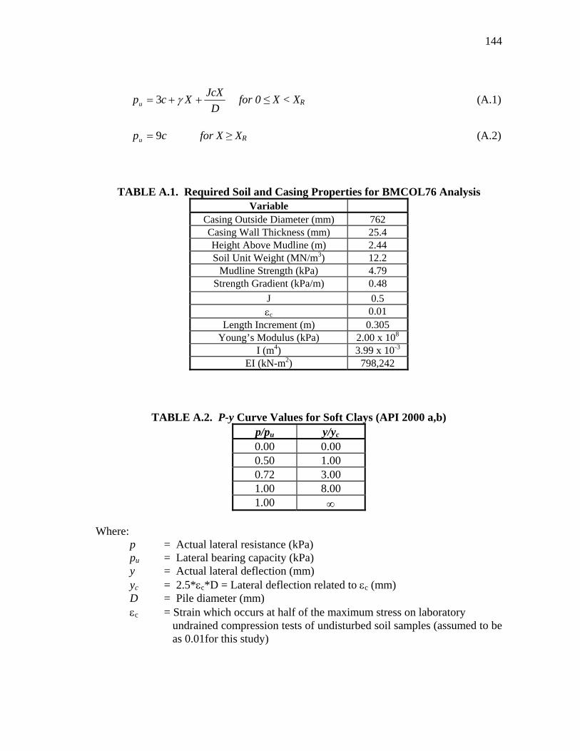
144

DJcXXcpu ++= γ3 for 0 ≤ X < XR (A.1)

cpu 9= for X ≥ XR (A.2)

TABLE A.1. Required Soil and Casing Properties for BMCOL76 Analysis Variable

Casing Outside Diameter (mm) 762 Casing Wall Thickness (mm) 25.4 Height Above Mudline (m) 2.44 Soil Unit Weight (MN/m3) 12.2

Mudline Strength (kPa) 4.79 Strength Gradient (kPa/m) 0.48

J 0.5 εc 0.01

Length Increment (m) 0.305 Young’s Modulus (kPa) 2.00 x 108

I (m4) 3.99 x 10-3

EI (kN-m2) 798,242

TABLE A.2. P-y Curve Values for Soft Clays (API 2000 a,b) p/pu y/yc

0.00 0.00 0.50 1.00 0.72 3.00 1.00 8.00 1.00 ∞

Where: p = Actual lateral resistance (kPa) pu = Lateral bearing capacity (kPa) y = Actual lateral deflection (mm) yc = 2.5*εc*D = Lateral deflection related to εc (mm) D = Pile diameter (mm) εc = Strain which occurs at half of the maximum stress on laboratory undrained compression tests of undisturbed soil samples (assumed to be as 0.01for this study)

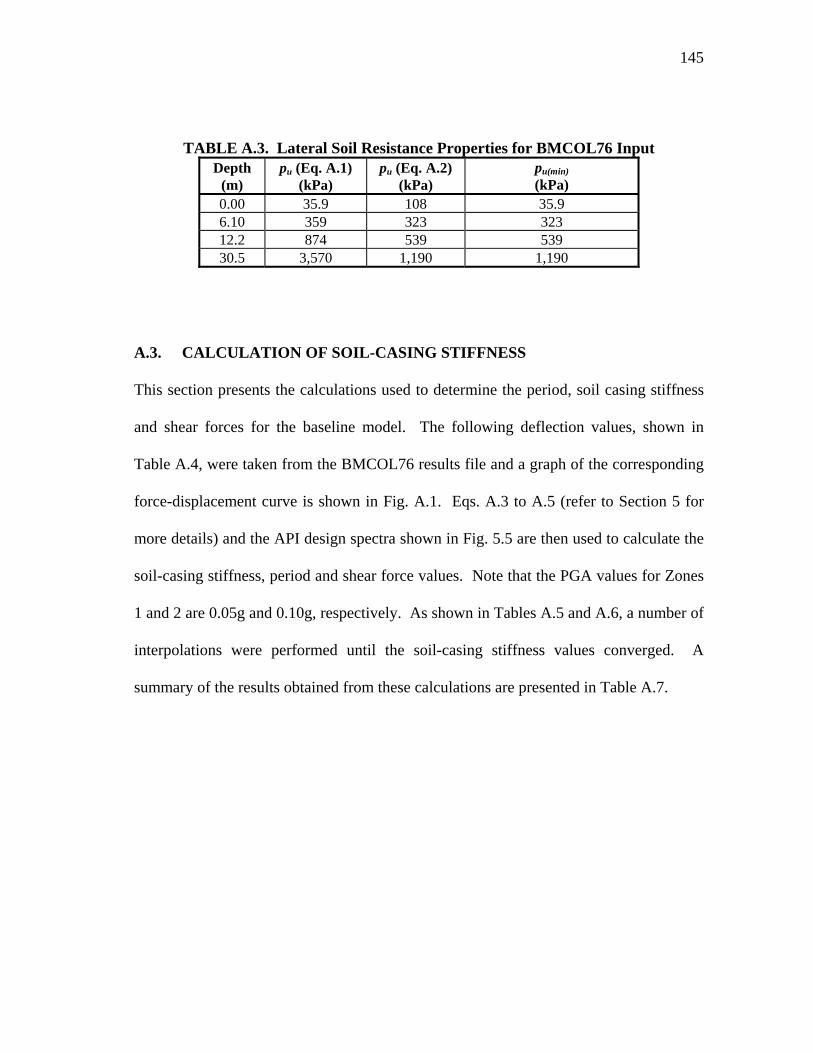
145

TABLE A.3. Lateral Soil Resistance Properties for BMCOL76 Input

Depth (m)

pu (Eq. A.1) (kPa)

pu (Eq. A.2) (kPa)

pu(min) (kPa)

0.00 35.9 108 35.9 6.10 359 323 323 12.2 874 539 539 30.5 3,570 1,190 1,190

A.3. CALCULATION OF SOIL-CASING STIFFNESS

This section presents the calculations used to determine the period, soil casing stiffness

and shear forces for the baseline model. The following deflection values, shown in

Table A.4, were taken from the BMCOL76 results file and a graph of the corresponding

force-displacement curve is shown in Fig. A.1. Eqs. A.3 to A.5 (refer to Section 5 for

more details) and the API design spectra shown in Fig. 5.5 are then used to calculate the

soil-casing stiffness, period and shear force values. Note that the PGA values for Zones

1 and 2 are 0.05g and 0.10g, respectively. As shown in Tables A.5 and A.6, a number of

interpolations were performed until the soil-casing stiffness values converged. A

summary of the results obtained from these calculations are presented in Table A.7.

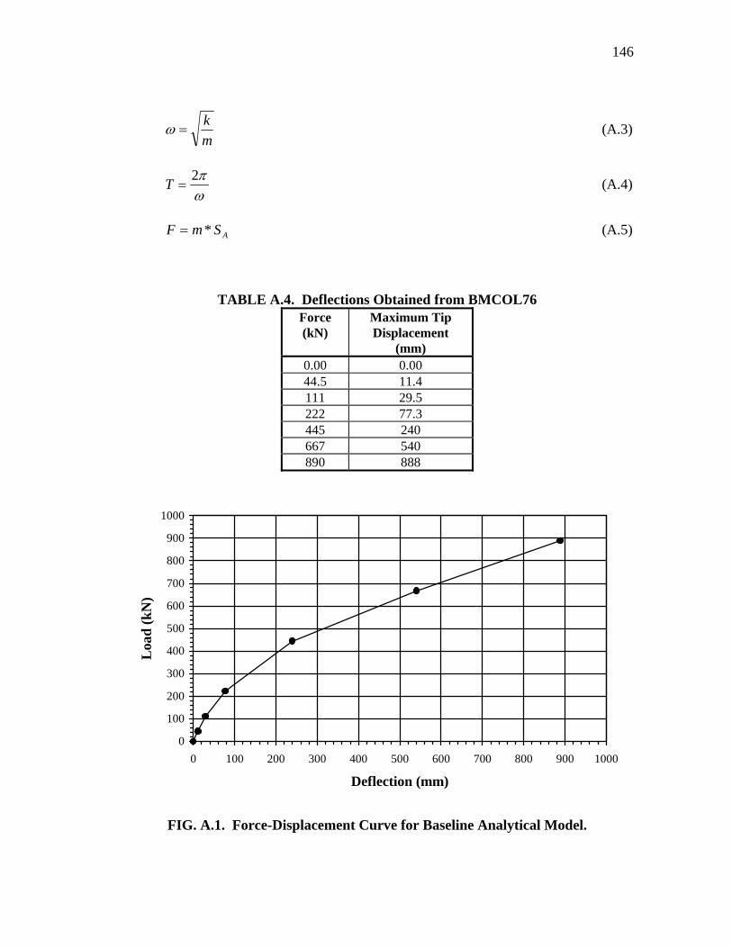
146

mk

=ω (A.3)

ωπ2

=T (A.4)

ASmF *= (A.5)

TABLE A.4. Deflections Obtained from BMCOL76 Force (kN)

Maximum Tip Displacement

(mm) 0.00 0.00 44.5 11.4 111 29.5 222 77.3 445 240 667 540 890 888

0

100

200

300

400

500

600

700

800

900

1000

0 100 200 300 400 500 600 700 800 900 1000

Deflection (mm)

Loa

d (k

N)

FIG. A.1. Force-Displacement Curve for Baseline Analytical Model.

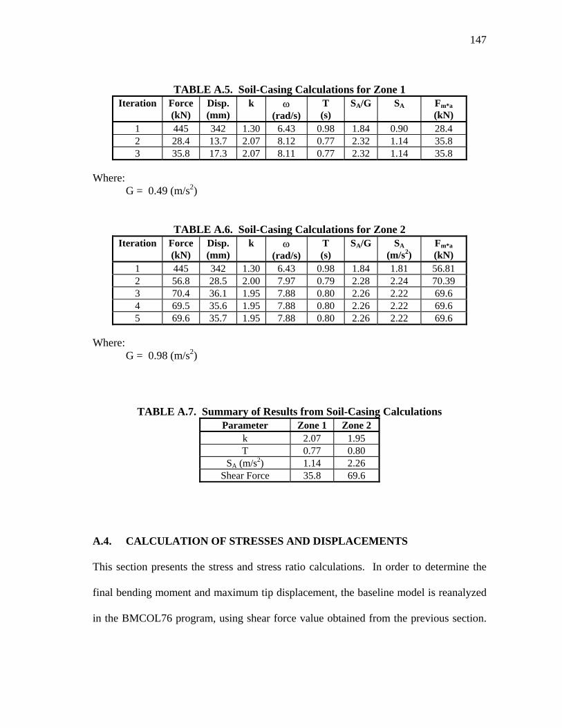
147

TABLE A.5. Soil-Casing Calculations for Zone 1 Iteration Force

(kN) Disp. (mm)

k ω (rad/s)

T (s)

SA/G SA Fm*a (kN)

1 445 342 1.30 6.43 0.98 1.84 0.90 28.4 2 28.4 13.7 2.07 8.12 0.77 2.32 1.14 35.8 3 35.8 17.3 2.07 8.11 0.77 2.32 1.14 35.8

Where: G = 0.49 (m/s2)

TABLE A.6. Soil-Casing Calculations for Zone 2 Iteration Force

(kN) Disp. (mm)

k ω (rad/s)

T (s)

SA/G SA (m/s2)

Fm*a (kN)

1 445 342 1.30 6.43 0.98 1.84 1.81 56.81 2 56.8 28.5 2.00 7.97 0.79 2.28 2.24 70.39 3 70.4 36.1 1.95 7.88 0.80 2.26 2.22 69.6 4 69.5 35.6 1.95 7.88 0.80 2.26 2.22 69.6 5 69.6 35.7 1.95 7.88 0.80 2.26 2.22 69.6

Where: G = 0.98 (m/s2)

TABLE A.7. Summary of Results from Soil-Casing Calculations Parameter Zone 1 Zone 2

k 2.07 1.95 T 0.77 0.80

SA (m/s2) 1.14 2.26 Shear Force 35.8 69.6

A.4. CALCULATION OF STRESSES AND DISPLACEMENTS

This section presents the stress and stress ratio calculations. In order to determine the

final bending moment and maximum tip displacement, the baseline model is reanalyzed

in the BMCOL76 program, using shear force value obtained from the previous section.

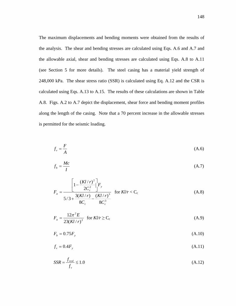
148

The maximum displacements and bending moments were obtained from the results of

the analysis. The shear and bending stresses are calculated using Eqs. A.6 and A.7 and

the allowable axial, shear and bending stresses are calculated using Eqs. A.8 to A.11

(see Section 5 for more details). The steel casing has a material yield strength of

248,000 kPa. The shear stress ratio (SSR) is calculated using Eq. A.12 and the CSR is

calculated using Eqs. A.13 to A.15. The results of these calculations are shown in Table

A.8. Figs. A.2 to A.7 depict the displacement, shear force and bending moment profiles

along the length of the casing. Note that a 70 percent increase in the allowable stresses

is permitted for the seismic loading.

AFfv = (A.6)

IMcfb = (A.7)

3

3

2

2

8)/(

8)/(33/5

2)/(1

cc

yc

a

CrKl

CrKl

FC

rKl

F−+

⎥⎦

⎤⎢⎣

⎡−

= for Kl/r < Cc (A.8)

2

2

)/(2312

rKlEFa

π= for Kl/r ≥ Cc (A.9)

yb FF 75.0= (A.10)

yv Ff 4.0= (A.11)

0.1≤=v

vcal

ff

SSR (A.12)

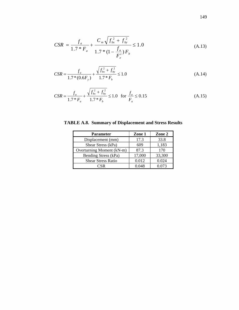
149

0.1)1(*7.1*7.1

22

≤

′−

++=

be

a

bybxm

a

a

FFf

ffC

Ff

CSR (A.13)

0.1*7.1)6.0(*7.1

22

≤+

+=b

bybx

y

a

F

ff

Ff

CSR (A.14)

0.1*7.1*7.1

22

≤+

+=b

bybx

a

a

F

ff

Ff

CSR for 15.0≤a

a

Ff

(A.15)

TABLE A.8. Summary of Displacement and Stress Results

Parameter Zone 1 Zone 2 Displacement (mm) 17.3 33.8 Shear Stress (kPa) 609 1,183

Overturning Moment (kN-m) 87.3 170 Bending Stress (kPa) 17,000 33,300

Shear Stress Ratio 0.012 0.024 CSR 0.048 0.073

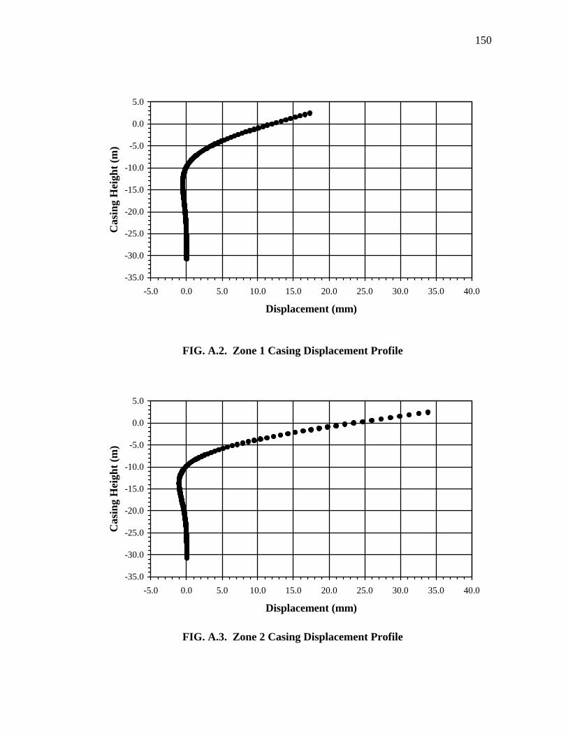
150

-35.0

-30.0

-25.0

-20.0

-15.0

-10.0

-5.0

0.0

5.0

-5.0 0.0 5.0 10.0 15.0 20.0 25.0 30.0 35.0 40.0

Displacement (mm)

Cas

ing

Hei

ght (

m)

FIG. A.2. Zone 1 Casing Displacement Profile

-35.0

-30.0

-25.0

-20.0

-15.0

-10.0

-5.0

0.0

5.0

-5.0 0.0 5.0 10.0 15.0 20.0 25.0 30.0 35.0 40.0

Displacement (mm)

Cas

ing

Hei

ght (

m)

FIG. A.3. Zone 2 Casing Displacement Profile

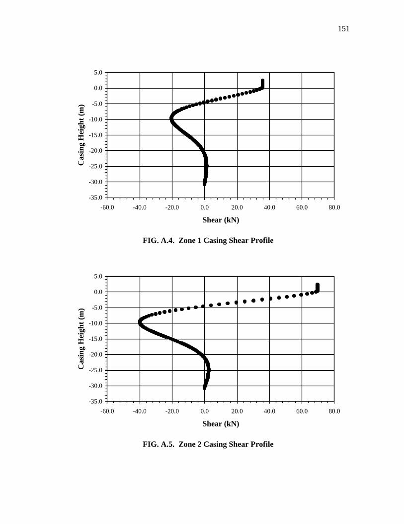
151

-35.0

-30.0

-25.0

-20.0

-15.0

-10.0

-5.0

0.0

5.0

-60.0 -40.0 -20.0 0.0 20.0 40.0 60.0 80.0

Shear (kN)

Cas

ing

Hei

ght (

m)

FIG. A.4. Zone 1 Casing Shear Profile

-35.0

-30.0

-25.0

-20.0

-15.0

-10.0

-5.0

0.0

5.0

-60.0 -40.0 -20.0 0.0 20.0 40.0 60.0 80.0

Shear (kN)

Cas

ing

Hei

ght (

m)

FIG. A.5. Zone 2 Casing Shear Profile

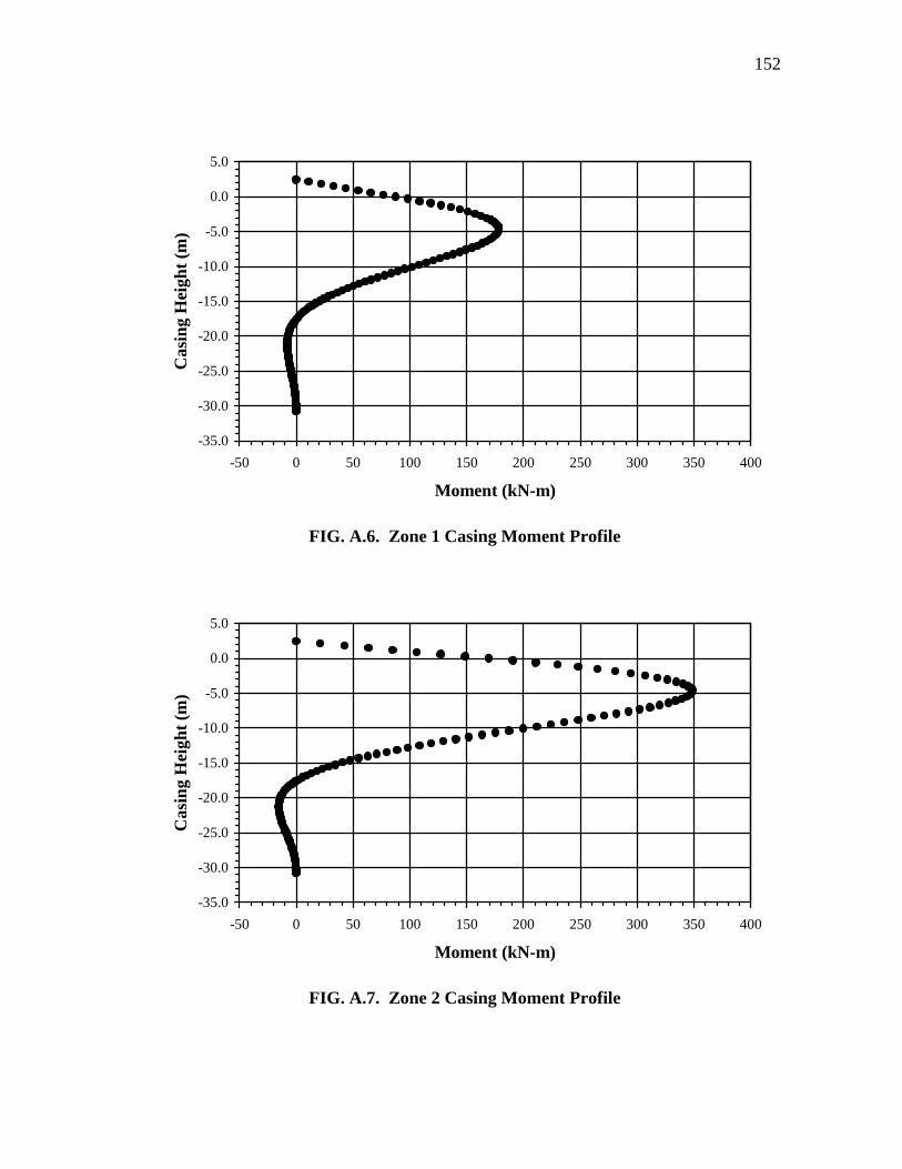
152

-35.0

-30.0

-25.0

-20.0

-15.0

-10.0

-5.0

0.0

5.0

-50 0 50 100 150 200 250 300 350 400

Moment (kN-m)

Cas

ing

Hei

ght (

m)

FIG. A.6. Zone 1 Casing Moment Profile

-35.0

-30.0

-25.0

-20.0

-15.0

-10.0

-5.0

0.0

5.0

-50 0 50 100 150 200 250 300 350 400

Moment (kN-m)

Cas

ing

Hei

ght (

m)

FIG. A.7. Zone 2 Casing Moment Profile

Documents

Assessment of Seismic Risk for Subsea Production … of Seismic Risk for Subsea Production Systems in the Gulf of Mexico by Laura Ann Brown, M.S., Texas A&M University Joseph M. Bracci,