Embed Size (px)
Citation preview
ASSESSMENT OF SLOPE STABILITY FOR A SEGMENT
(Km: 25+600-26+000) OF ANTALYA-KORKUTELİ HIGHWAY
A THESIS SUBMITTED TO THE GRADUATE SCHOOL OF NATURAL AND APPLIED SCIENCES
OF
MIDDLE EAST TECHNICAL UNIVERSITY
BY
HURİYE ASLI ARIKAN
IN PARTIAL FULFILLMENT OF THE REQUIREMENTS FOR
THE DEGREE OF MASTER OF SCIENCE IN
GEOLOGICAL ENGINEERING DEPARTMENT
JUNE 2010

ii

iii
I hereby declare that all information in this document has been obtained and presented in accordance with academic rules and
ethical conduct. I also declare that, as required by these rules and conduct, I have fully cited and referenced all material and results that are not original to this work.
Name, Last name : Huriye Aslı Arıkan
Signature :
iv
ABSTRACT
ASSESSMENT OF SLOPE STABILITY FOR A SEGMENT
(KM: 25+600-26+000) OF ANTALYA-KORKUTELĠ HIGHWAY
Arıkan, Huriye Aslı
M.Sc., Department of Geological Engineering
Supervisor: Prof. Dr. Tamer Topal
June 2010, 94 pages
The cut slopes at a segment between Km 25+600 and 26+000 of the
Antalya-Burdur Breakaway-Korkuteli State Road to be newly constructed
have slope instability problems due to the existence of highly jointed
limestone.
The purpose of this study is to investigate the engineering geological
properties of the units exposed at three cut slopes, to assess stability of
the cut slopes, and to recommend remedial measures for the problematic
sections.
In this respect, both field and laboratory studies have been carried out.
The limestone exposed at the cut slopes are beige to gray, fine grained,
fossiliferous, and highly jointed. It has two joint sets and a bedding plane
v
as main discontinuities. The kinematic analysis indicates that planar failure
is expected at Km: 25+900. Limit equilibrium analysis show that the cut
slopes with bench have no slope instability problems except rockfalls
which endanger the traffic safety. In this thesis it is recommended to
covering the cut slope with wire mesh and fibre reinforced shotcrete
Keywords: Highway, Limestone, Kinematic Analysis, Limit Equilibrium
Analysis, Rock-Fall, Rock Slope, Korkuteli
vi
ÖZ
ANTALYA-KORKUTELĠ KARAYOLUNUN BĠR KESĠMĠ (KM: 25+600-
26+000) ĠÇĠN ġEV DURAYLILIĞININ DEĞERLENDĠRĠLMESĠ
Arıkan, Huriye Aslı
Yüksek Lisans, Jeoloji Mühendisliği Bölümü
Tez Yöneticisi: Prof. Dr. Tamer Topal
Haziran 2010, 94 sayfa
Yeni yapılacak Antalya-Burdur Ayrımı Korkuteli Yolunun Km:25+500-
26+000 arasındaki kesiminde bulunan ve çok çatlaklı kireçtaĢı içinde yer
alan kaya yarma Ģevlerinde, Ģev duraysızlık problemleri bulunmaktadır.
Bu çalıĢmanın amacı, kaya yarma Ģevlerde bununan birimlerin mühendislik
jeolojisi özelliklerini incelemek, Ģev stabilitesini değerlendirmek ve
problemli kesimler için çözüm önermektir.
Bu çerçevede, saha ve laboratuvar çalıĢmaları yapılmıĢtır. Kaya yarma
Ģevlerde, bej-gri, ince taneli fosilli ve çok çatlaklı kireçtaĢı bulunmaktadır.
Ana süreksizlikler olarak, kayaçta iki eklem takımı ve bir tabaka
mevcuttur. Yapılan kinematik analizlere göre, Km: 25+900’de düzlemsel
vii
kayma beklenmektedir. Trafik güvenliğini tehlikeye düĢürecek kaya
düĢmeleri dıĢında, limit denge analizlerine göre palyeli Ģevlerde herhangi
bir duraysızlık problemi bulunmamaktadır. Bu tezde, palyeli kaya yarma
Ģevler için, tel kafes ve fiberle güçlendirimiĢ Ģatkrit kullanılması
önerilmektedir.
Anahtar kelimeler: Karayolu, KireçtaĢı, Kinematik Analiz, Limit Denge
Analizi, Kaya DüĢmesi, Kaya ġevi, Korkuteli

viii
To My Dear Mother, Father and My Grandfather

ix
ACKNOWLEDGEMENTS
I am greatly indebted to Prof.Dr. Tamer Topal for his guidance, very
encouraging supervision, interest, patience and his endless helps.
Many thanks to all my instructors for giving the best information.
I am grateful to Geol. Eng. Tahir Tanju Ökten and Geol. Eng. Mehmet
Besim Hanedar at Form-Beril for their support during the thesis studies, all
the field work studies, the laboratory supports and information and
knowledge sharing.
I want to thank to my dear friend Esin ġiĢman for her help, productive
suggestions and discussions, especially in the research part. Also for her
friendship and all kinds of helps and supports for years.
I would like to thank to all my friends, especially UlaĢ Canatalı, Balkın
Çoker and Nazan Çapoğlu for all their supports and helps and especially
their friendship during the stressful preparation stage.
Finally, I would like to thank my family, my mom and dad, for their
unlimited patience, support and encouragement in every step I took both
in this study and all through my life. I also would like to thank to my
grandfather and my grandmother for their support and willingness for
finishing this degree.
x
TABLE OF CONTENTS
ABSTRACT……………………………………………………………………………………………………iv
ÖZ………………………………………………………………………………………………………………vi
ACKNOWLEDGEMENTS…………………………………………………………………………………ix
TABLE OF CONTENTS……………………………………………………………………………………x
LIST OF TABLES…………………………………………………………………………………………xiii
LIST OF FIGURES………………………………………………………………………………………xiv
CHAPTER
1. INTRODUCTION……………………………………………………………………………………1
1.1. Purpose and Scope…………………………………………………………………1
1.2. Location and Properties of the Road…………………………………………2
1.3. Vegetation and Climate……………………………………………………………5
1.4. Methods of Study……………………………………………………………………7
1.5. Previous Studies………………………………………………………………………8
2. GEOLOGY AND SEISMICITY OF THE STUDY AREA……………………………10
2.1. Geology of the Study Area……………………………………………………10
2.2. Seismicity of the Study Area…………………………………………………13
3. ENGINEERING GEOLOGICAL PROPERTIES OF THE LIMESTONE
xi
EXPOSED AT Km: 25+600-26+000…………………………………………………16
3.1. Engineering Geological Properties of Limestone at Km:
25+600………………………………………………………………………………23
3.2. Engineering Geological Properties of Limestone at Km:
25+900…………………………………………………………………………………27
3.3. Engineering Geological Properties of Limestone at Km:
26+000…………………………………………………………………………………31
4. KINEMATIC ANALYSES OF THE CUT SLOPES……………………………………35
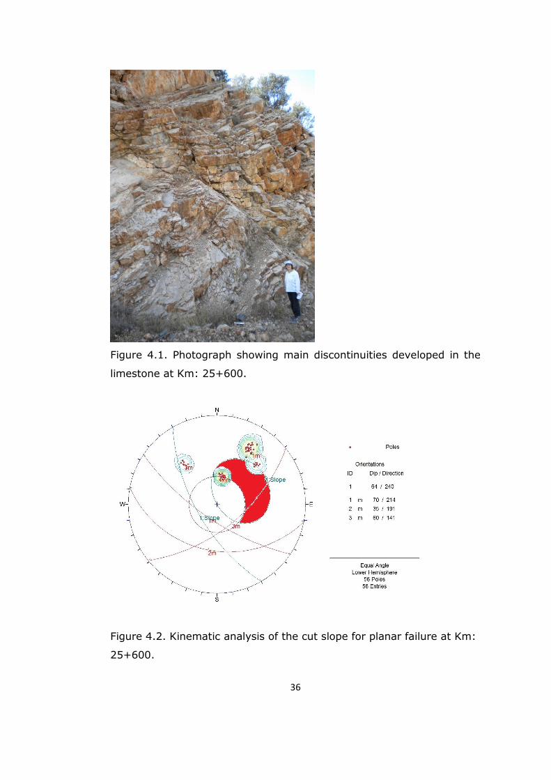
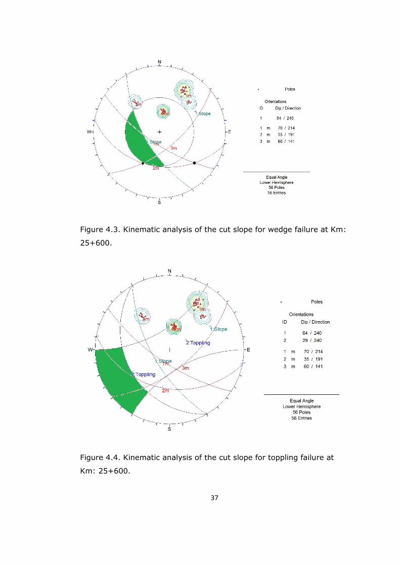
4.1. Kinematic Analysis of the Cut Slope at Km: 25+600…………35
4.2. Kinematic Analysis of the Cut Slope at Km: 25+900…………38
4.3. Kinematic Analysis of the Cut Slope at Km: 26+000…………42
5. LIMIT EQUILIBRIUM AND ROCKFALL ANALYSES OF THE SLOPE ……45
5.1. Limit Equilibrium Analysis of the Cut Slope for Planar Failure
at Km: 25+900………………………………………………………………………46
5.2. Limit Equilibrium Analysis of the Cut Slope for Mass Failure at
Km: 25+900………………………………………………………………………46
5.3. Rockfall Analysis of the Cut Slope………………………………………58
5.3.1. Rockfall Analysis of the Cut Slopes in the Current
Situation……………………………………………………………………58
5.3.2. Rockfall Analysis of the Cut Slope at Km: 25+600……62
5.3.3. Rockfall Analysis of the Cut Slope at Km: 25+900……69
5.3.4. Rockfall Analysis of the Cut Slope at Km: 26+000……76

xii
6. DISCUSSION……………………………………………………………………………………84
7. CONCLUSIONS AND RECOMMENDATIONS………………………………………90
REFERENCES……………………………………………………………………………………………92
xiii
LIST OF TABLES
TABLE
Table 3.1. Orientations of the major discontinuity sets at Km:25+600…26
Table 3.2. Orientations of the major discontinuity sets at Km:25+900…28
Table 3.3. Orientations of the major discontinuity sets at Km:26+000…32
Table 5.1. Parameters used in the rockfall analysis for the cut slopes…58
Table 6.1. Comparison of the factor of safety values from the limit
equilibrium analysis at Km: 25+900……………………………………85
Table 6.2. Rockfall run-out distances for the cut slopes………………………86
Table 6.3. Types of rockfall movements at the cut slopes ……………………87
Table 6.4. Comparison of the catch barrier distances from the road ……88
xiv
LIST OF FIGURES
FIGURES
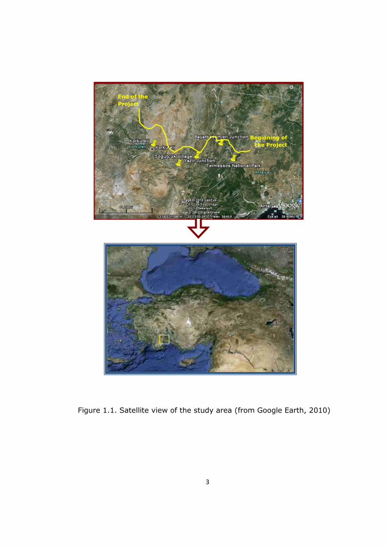
Figure 1.1. Satellite view of the study area………………………………………………3
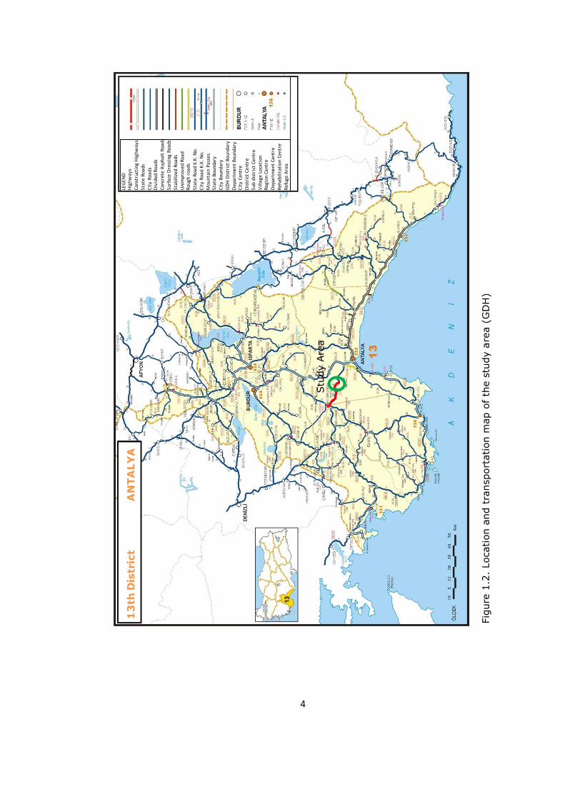
Figure 1.2. Location and transportation map of the study Area………………4
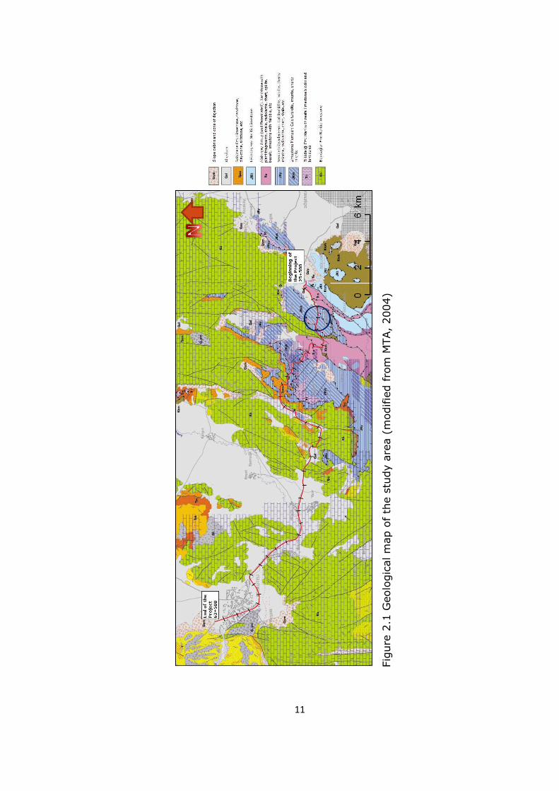
Figure 2.1. Geological map of the study area (modified from MTA)………11
Figure 2.2. A view from Yeniceboğazıdere formation……………………………12
Figure 2.3. A view from Limestone Unit…………………………………………………13
Figure 2.4. Earthquake zoning map of the study area and its close
vicinity with recorded epicenters …………………………………………34
Figure 2.5. Earthquake acceleration map of Turkey for the stability
analyses of slopes…………………………………………………………………35
Figure 3.1. The geological plan (Scale: 1/1000) showing the borehole
(SK-1 and SK-2) locations near Yenice bridge at Km:
26+600-26+700)…………………………………………………………………17
Figure 3.2. Borehole log of SK-1 at Yenice bridge…………………………………18
Figure 3.3. Borehole log of SK-2 at Yenice bridge…………………………………19
Figure 3.4. Photograph of the oriented samples taken from the field……19
Figure 3.5. Summary report for the direct shear test……………………………21
Figure 3.6. Mohr-Coulomb failure criterion of the limestone based the
xv
test results……………………………………………………………………………22
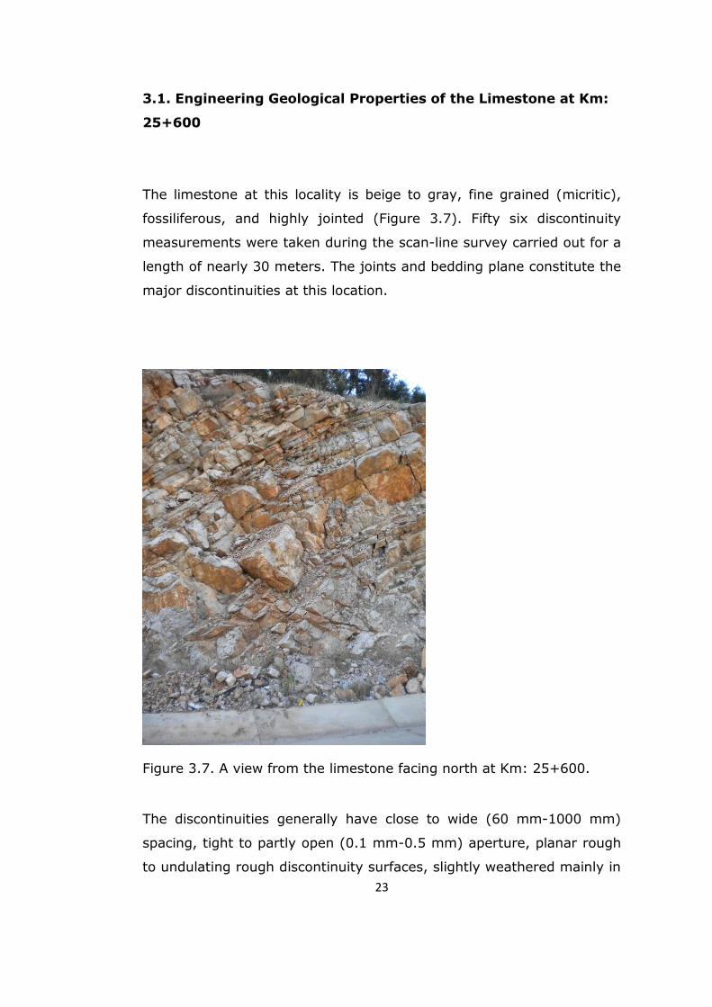
Figure 3.7. A view from limestone facing north at Km: 25+600……………23
Figure 3.8. Pole plot and contour diagram of the discontinuities at Km:
25+600…………………………………………………………………………………24
Figure 3.9. Rose diagram of the discontinuities at Km: 25+600……………25
Figure 3.10. Dominant discontinuity sets at Km: 25+600……………………25
Figure 3.11. A view from the limestone facing north at Km: 25+600……26
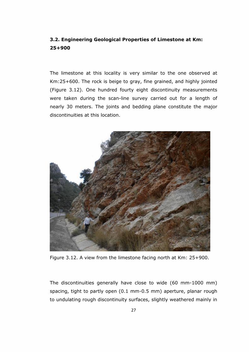
Figure 3.12. A view from the limestone facing north at Km: 25+900……27
Figure 3.13. Pole plot and contour diagram of the discontinuities at Km:
25+900………………………………………………………………………………29
Figure 3.14. Rose diagram of the discontinuities at Km: 25+900…………29
Figure 3.15. Dominant discontinuity sets at Km: 25+900……………………30
Figure 3.16. A view from the limestone at Km: 25+900………………………30
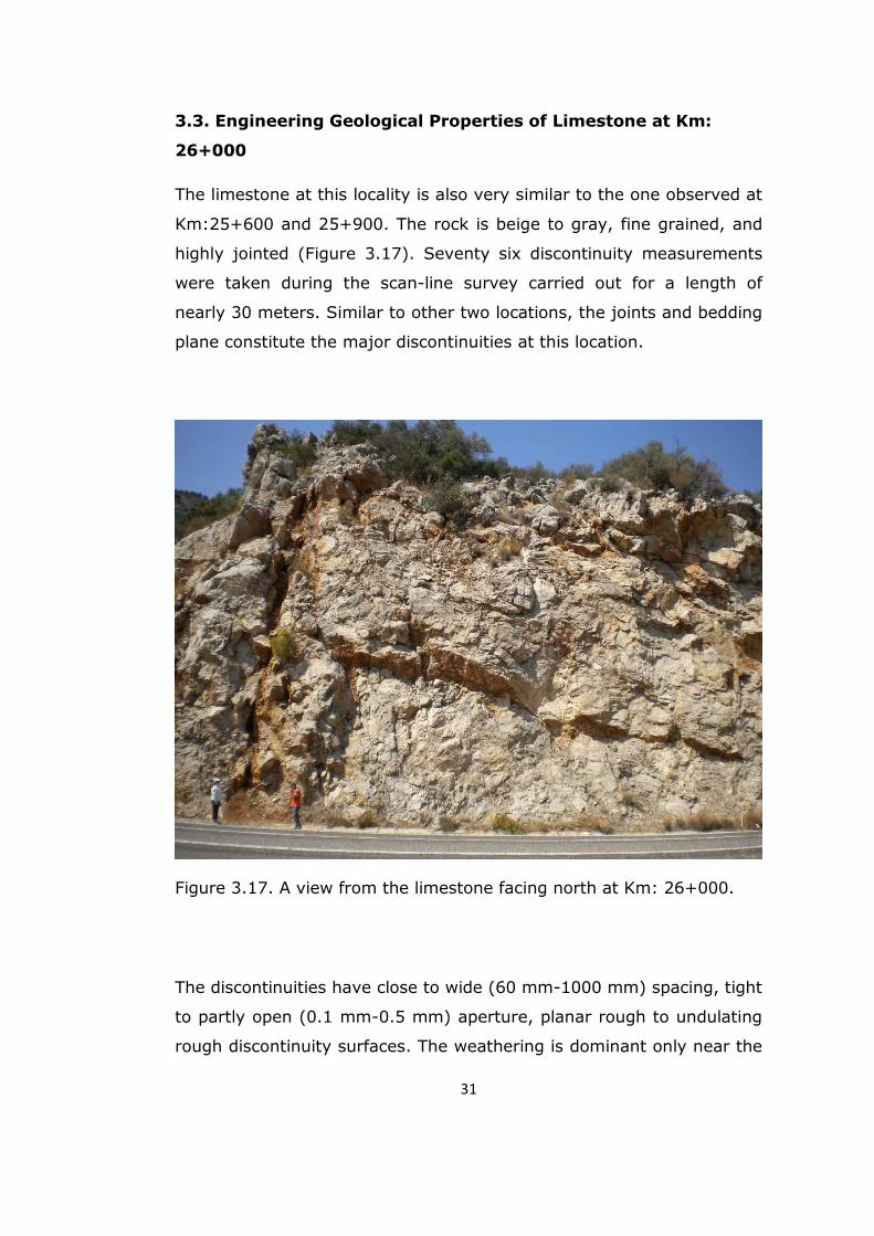
Figure 3.17. A view from the limestone facing north at Km: 26+000……31
Figure 3.18. Pole plot and contour diagram of the discontinuities at Km:
26+000………………………………………………………………………………33
Figure 3.19. Rose diagram of the discontinuities at Km: 26+000…………33
Figure 3.20. Dominant discontinuity sets at Km: 26+000……………………34
Figure 3.21. Discontinuities developed in the limestone at Km: 26+000
……………………………………………………………………………………………34
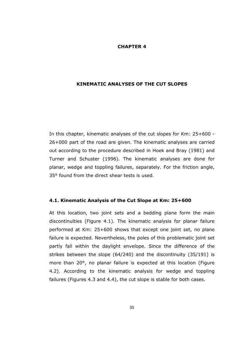
Figure 4.1. Photograph showing main discontinuities developed in the
xvi
limestone at Km: 25+600……………………………………………………36
Figure 4.2. Kinematic analysis of the cut slope for planar failure at Km:
25+600…………………………………………………………………………………36
Figure 4.3. Kinematic analysis of the cut slope for wedge failure at Km:
25+600…………………………………………………………………………………37
Figure 4.4. Kinematic analysis of the cut slope for toppling failure at Km:
25+600…………………………………………………………………………………37
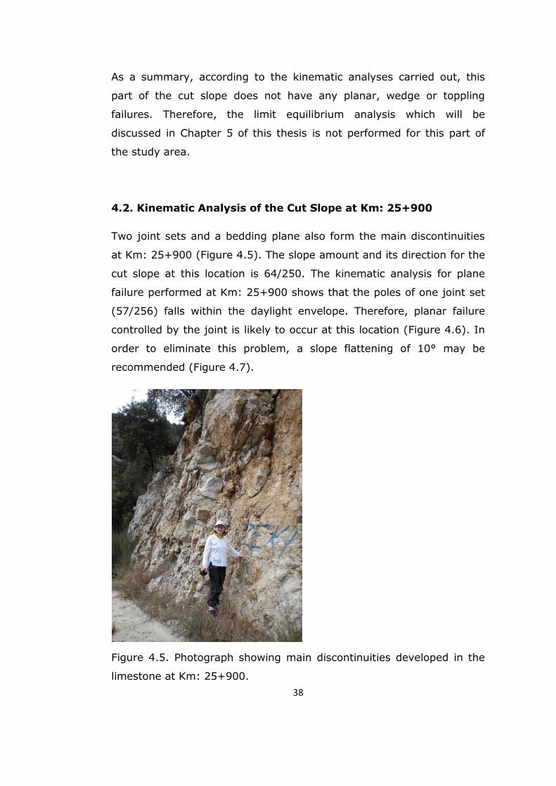
Figure 4.5. Photograph showing main discontinuities developed in the
limestone at Km: 25+900……………………………………………………38
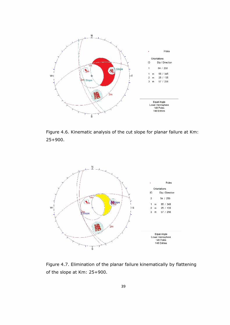
Figure 4.6. Kinematic analysis of the cut slope for planar failure at Km:
25+900…………………………………………………………………………………39
Figure 4.7. Elimination of the planar failure kinematically by flattening of
the slope at Km: 25+900………………………………………………………39
Figure 4.8. Kinematic analysis of the cut slope for wedge failure at Km:
25+900…………………………………………………………………………………40
Figure 4.9. Elimination of the wedge failure kinematically by flattening of
the slope at Km: 25+900………………………………………………………41
Figure 4.10. Kinematic analysis of the cut slope for toppling failure at
Km: 25+900……………………………………………………………………41
Figure 4.11. Photograph showing main discontinuities developed in the
limestone at Km: 26+000…………………………………………………42
Figure 4.12. Kinematic analysis of the cut slope for planar failure at Km:
26+000………………………………………………………………………………43
xvii
Figure 4.13. Kinematic analysis of the cut slope for wedge failure at Km:
26+000………………………………………………………………………………44
Figure 4.14. Kinematic analysis of the cut slope for toppling failure at
Km: 26+000………………………………………………………………………44
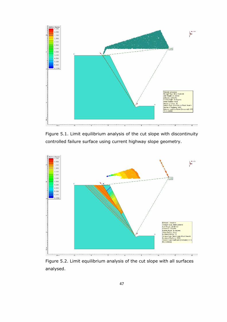
Figure 5.1. Limit equilibrium analysis of the cut slope with discontinuity
controlled failure surface using current highway slope
geometry………………………………………………………………………………47
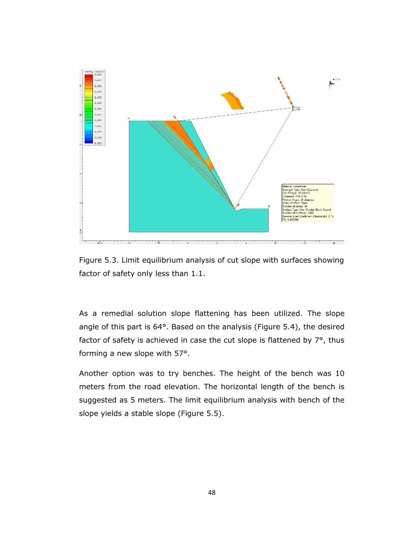
Figure 5.2. Limit equilibrium analysis of the cut slope with all surfaces
analysed…………………………………………………………………………………47
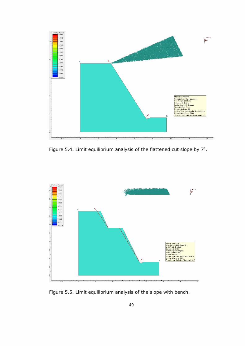
Figure 5.3. Limit equilibrium analysis of cut slope with surfaces showing
factor of safety only less than 1.1………………………………………48
Figure 5.4. Limit equilibrium analysis of the flattened cut slope by 7o…49
Figure 5.5. Limit equilibrium analysis of the slope with bench……………49
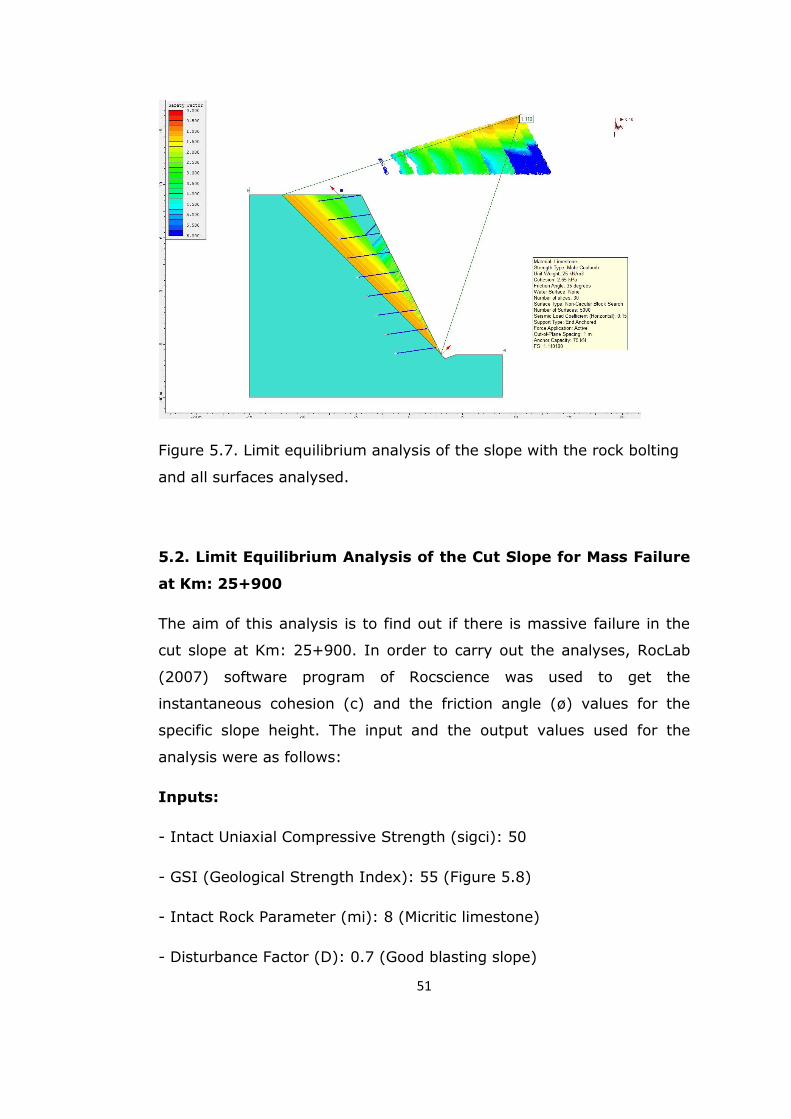
Figure 5.6. Limit equilibrium analysis of the slope with rock bolting…50
Figure 5.7. Limit equilibrium analysis of the slope with the rock bolting
and all surfaces analysed………………………………………………………48
Figure 5.8. GSI value of the limestone rock mass selected from the
Roclab software……………………………………………………………………52
Figure 5.9. The outputs of RocLab software for cut slope analyzed………53
Figure 5.10. Limit equilibrium analysis of the cut slope for mass failure
with current slope geometry……………………………………………………………………54
Figure 5.11. Limit equilibrium analysis of the cut slope for mass failure
with all possible failure surfaces……………………………………………………………54
xviii
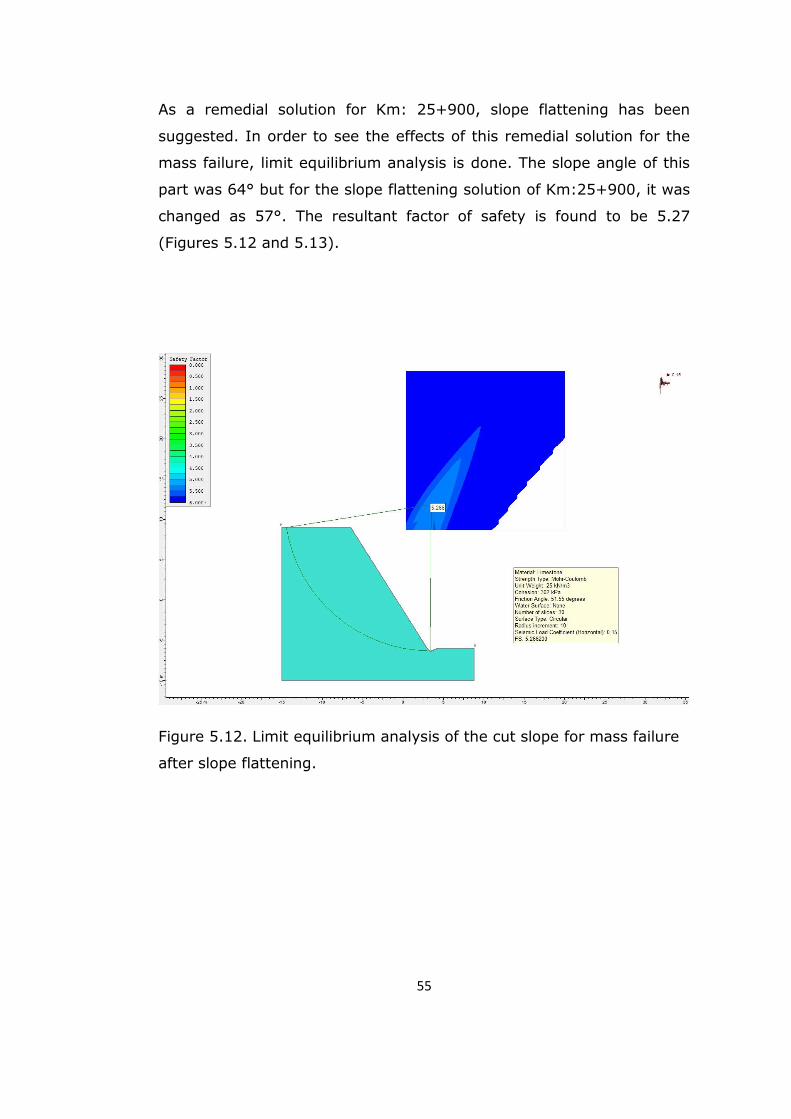
Figure 5.12. Limit equilibrium analysis of the cut slope for mass failure
after slope flattening…………………………………………………………55
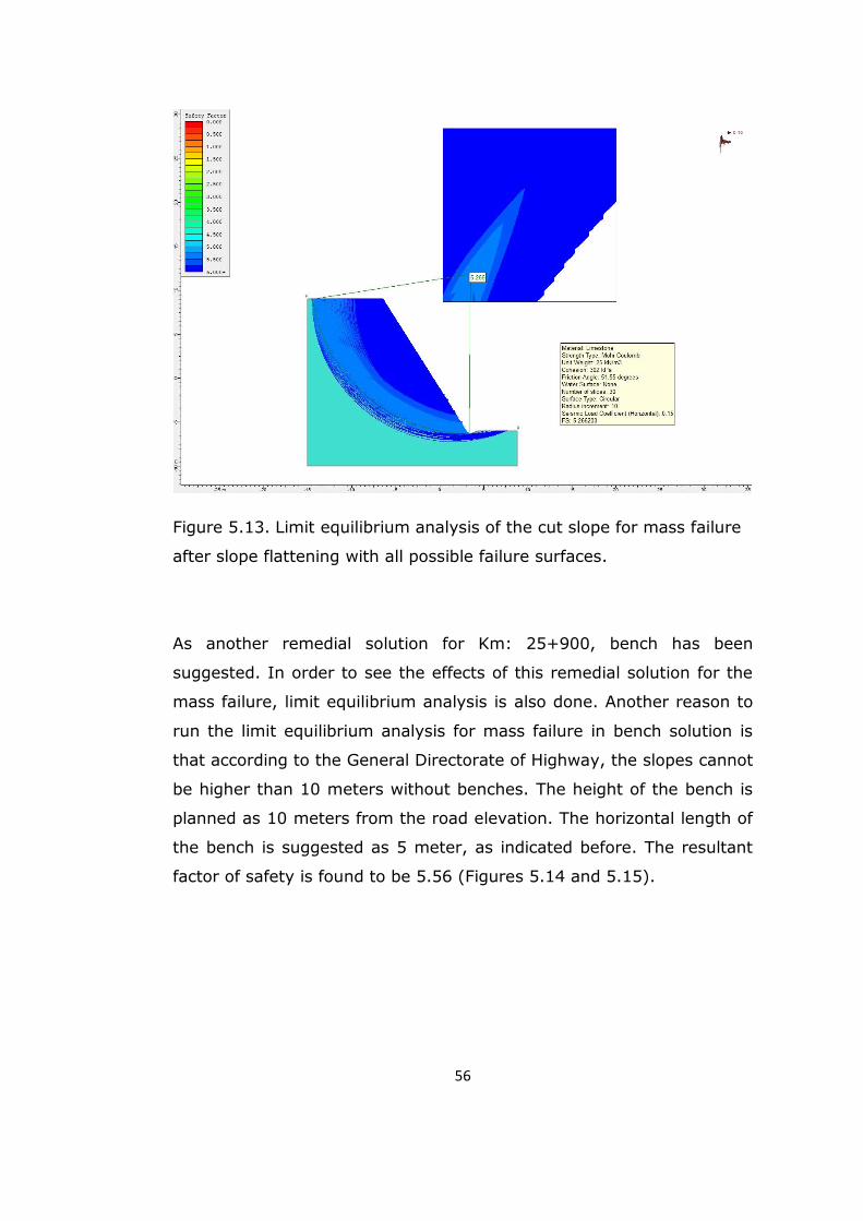
Figure 5.13. Limit equilibrium analysis of the cut slope for mass failure
after slope flattening with all possible failure surfaces ……56
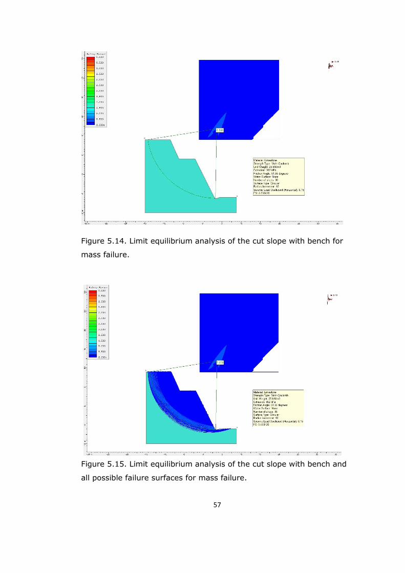
Figure 5.14. Limit equilibrium analysis of the cut slope with bench for
mass failure………………………………………………………………………57
Figure 5.15. Limit equilibrium analysis of the cut slope with bench and all
possible failure surfaces for mass failure…………………………57
Figure 5.16. Rockfall analysis with 10 kg block for current slope condition
……………………………………………………………………………………………59
Figure 5.17. Rockfall analysis with 60 kg block for current slope condition
……………………………………………………………………………………………59
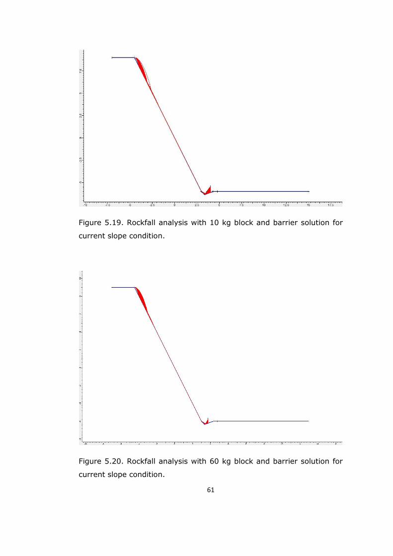
Figure 5.18. Rockfall analysis with 150 kg block for current slope
condition……………………………………………………………………………60
Figure 5.19. Rockfall analysis with 10 kg block and barrier solution for
current slope condition………………………………………………………61
Figure 5.20. Rockfall analysis with 60 kg block and barrier solution for
current slope condition………………………………………………………61
Figure 5.21. Rockfall analysis with 150 kg block and barrier solution for
current slope condition………………………………………………………62
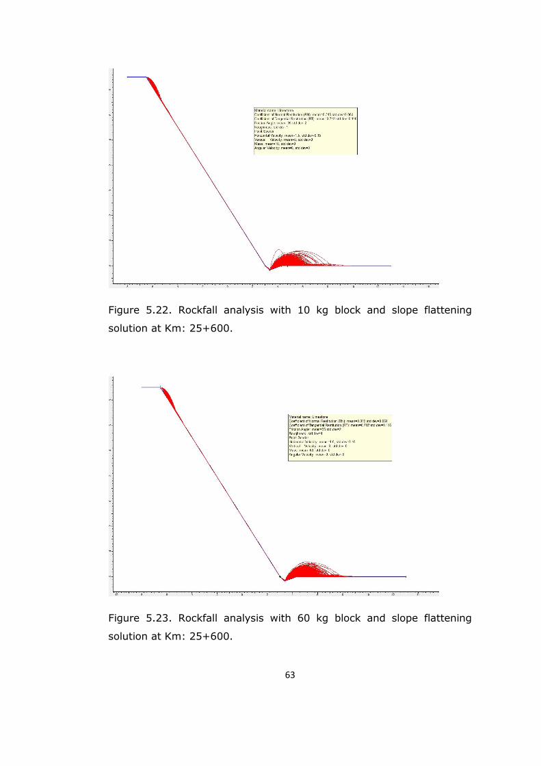
Figure 5.22. Rockfall analysis with 10 kg block and slope flattening
solution at Km: 25+600……………………………………………………63
Figure 5.23. Rockfall analysis with 60 kg block and slope flattening
solution at Km: 25+600……………………………………………………63
xix
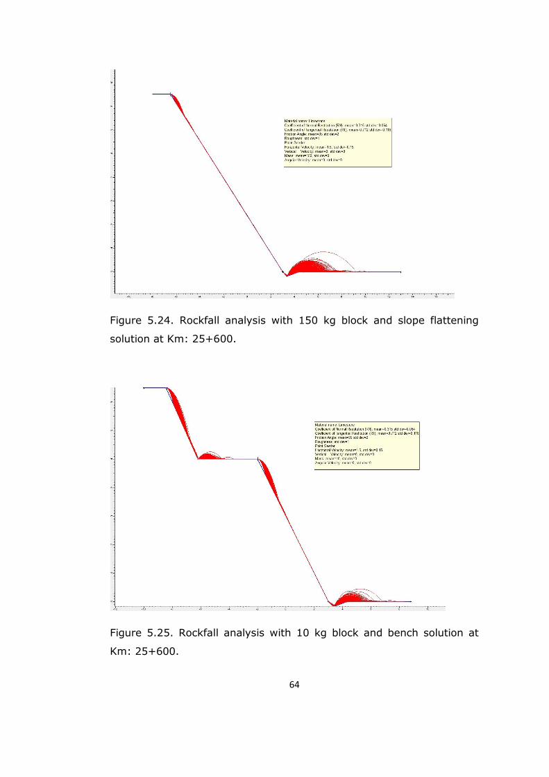
Figure 5.24. Rockfall analysis with 150 kg block and slope flattening
solution at Km: 25+600……………………………………………………64
Figure 5.25. Rockfall analysis with 10 kg block and bench solution at Km:
25+600………………………………………………………………………………64
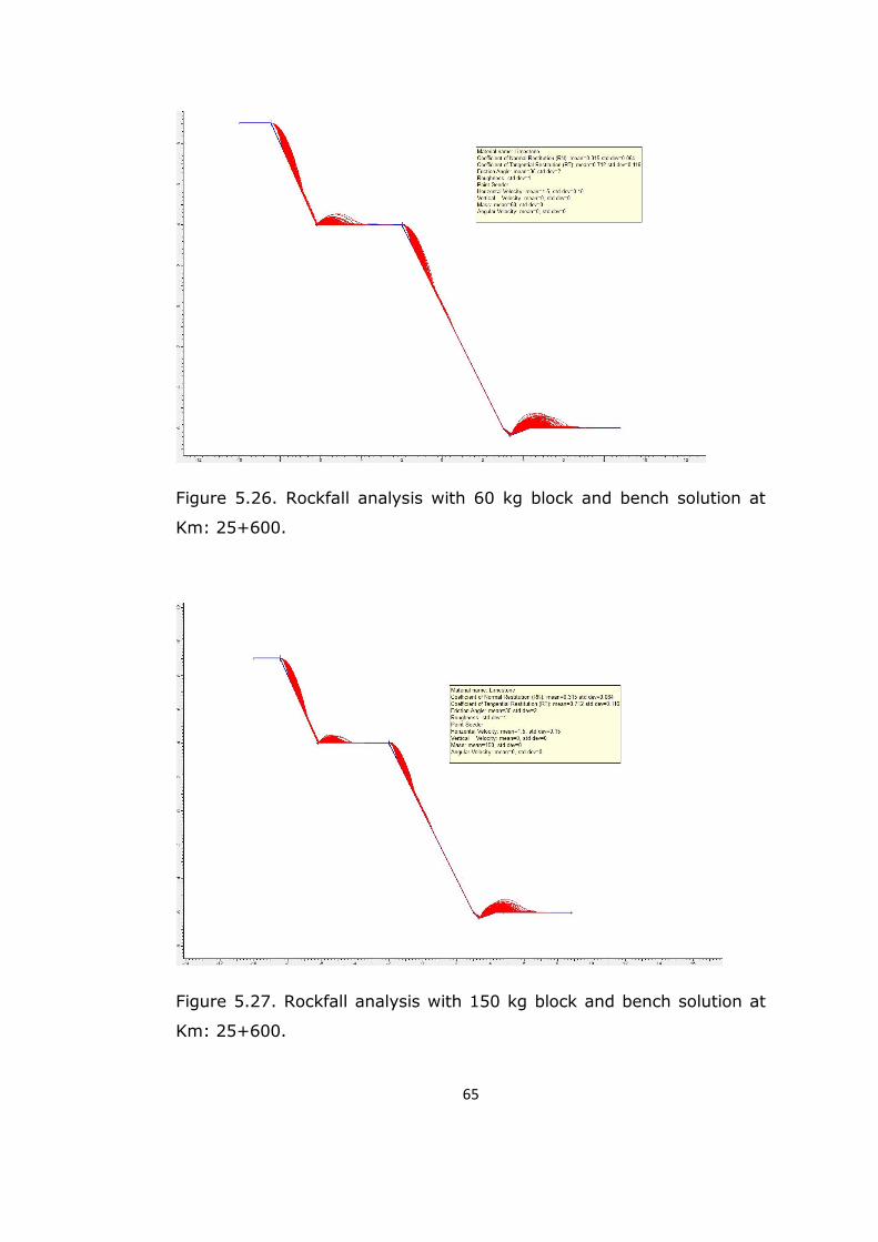
Figure 5.26. Rockfall analysis with 60 kg block and bench solution at Km:
25+600………………………………………………………………………………65
Figure 5.27. Rockfall analysis with 150 kg block and barrier solution for
current slope condition………………………………………………………65
Figure 5.28. Rockfall analysis (10 kg block) with slope flattening and
barrier solution at Km: 25+600………………………………………66
Figure 5.29. Rockfall analysis (60 kg block) with slope flattening and
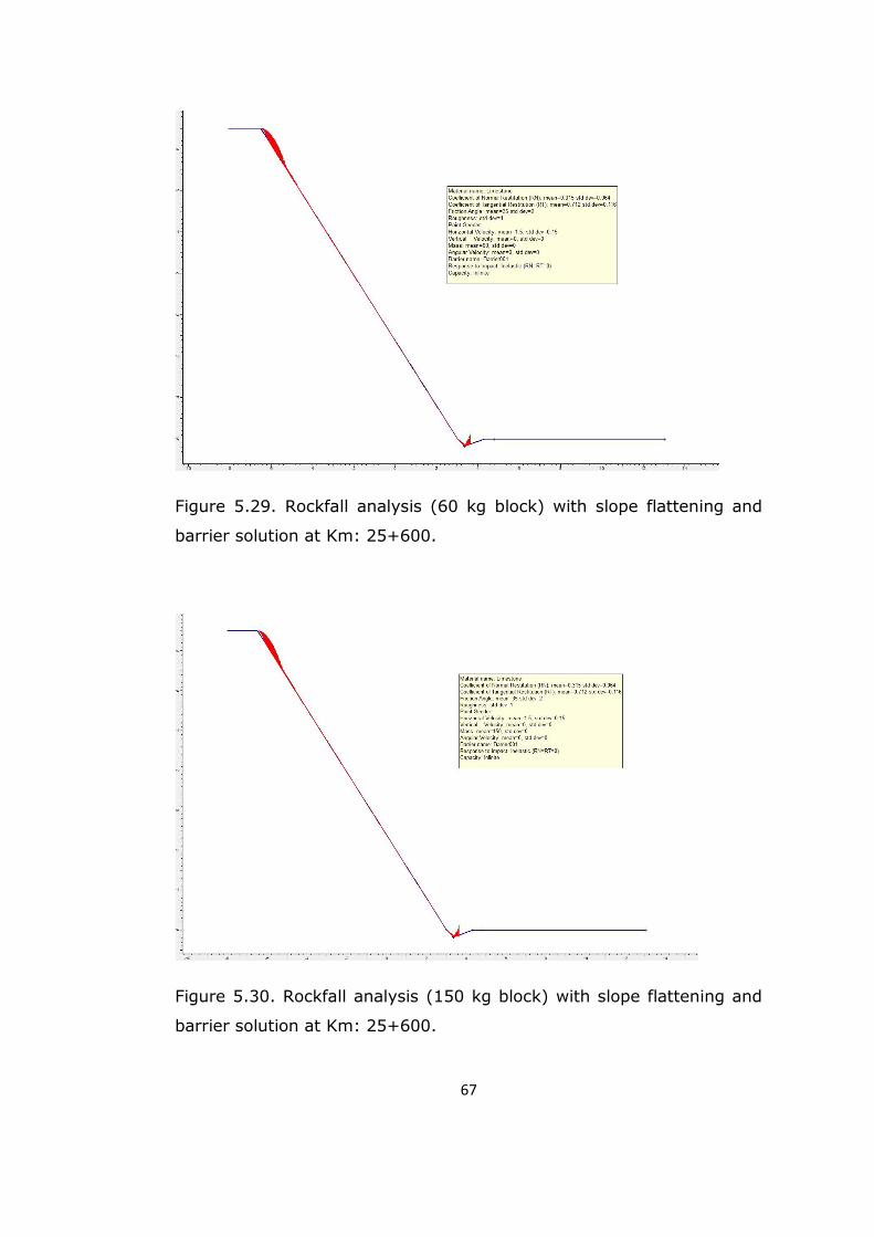
barrier solution at Km: 25+600………………………………………67
Figure 5.30. Rockfall analysis (150 kg block) with slope flattening and
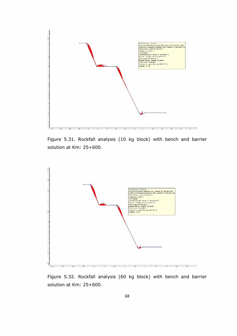
barrier solution at Km: 25+600………………………………………67
Figure 5.31. Rockfall analysis (10 kg block) with bench and barrier
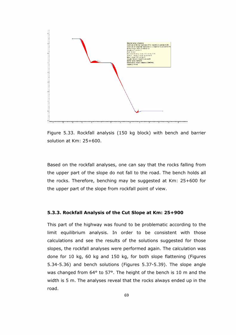
solution at Km: 25+600……………………………………………………68
Figure 5.32. Rockfall analysis (60 kg block) with bench and barrier
solution at Km: 25+600……………………………………………………68
Figure 5.33. Rockfall analysis (150 kg block) with bench and barrier
solution at Km: 25+600……………………………………………………69
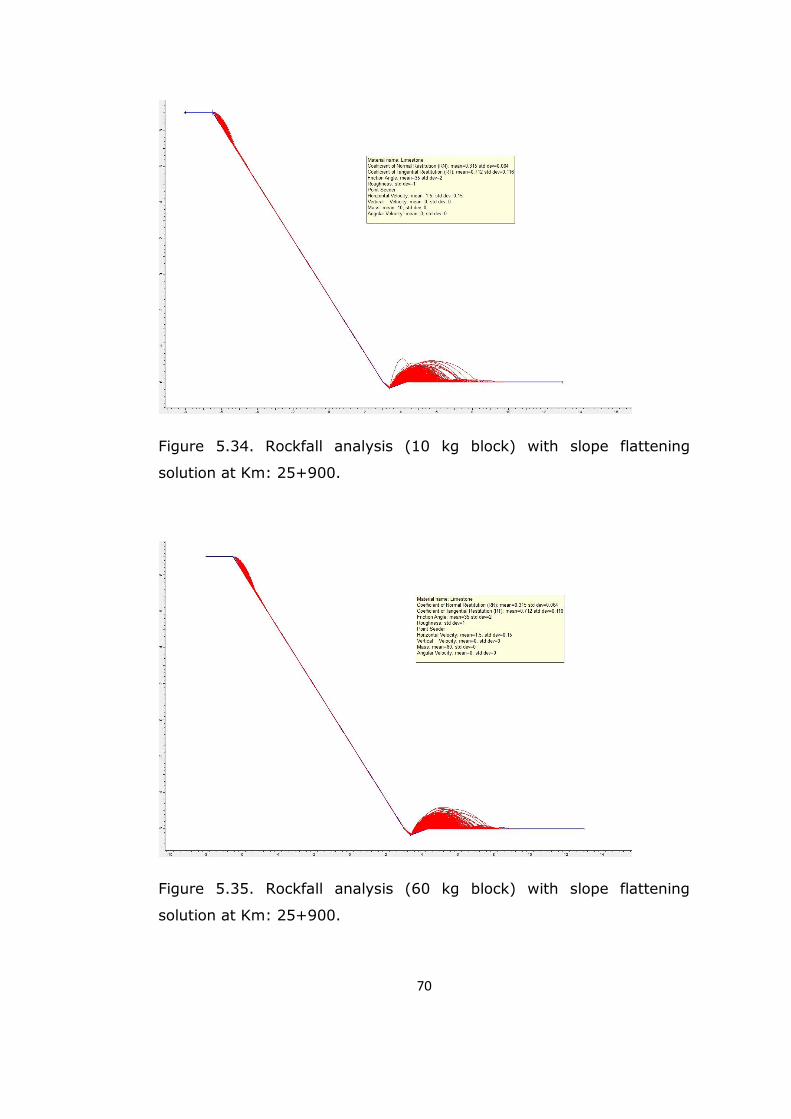
Figure 5.34. Rockfall analysis (10 kg block) with slope flattening solution
at Km: 25+900……………………………………………………………………70
xx
Figure 5.35. Rockfall analysis (60 kg block) with slope flattening solution
at Km: 25+900……………………………………………………………………70
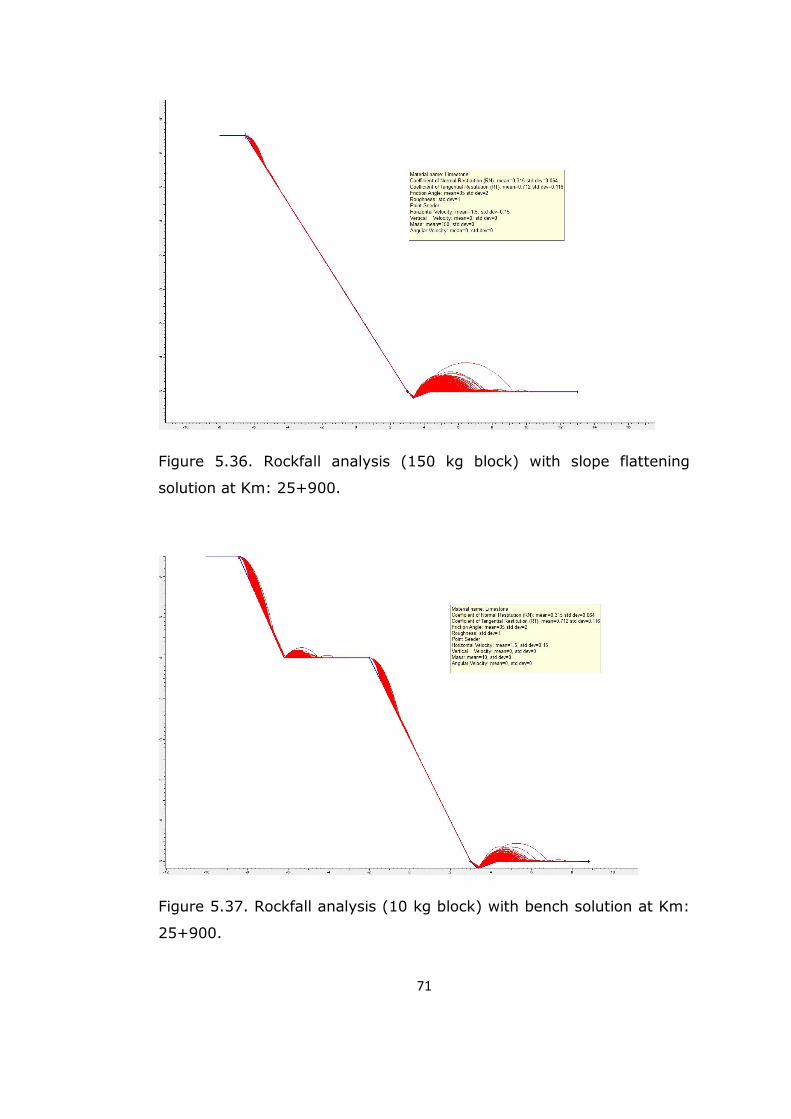
Figure 5.36. Rockfall analysis (150 kg block) with slope flattening
solution at Km: 25+900……………………………………………………71
Figure 5.37. Rockfall analysis (10 kg block) with bench solution at Km:
25+900………………………………………………………………………………71
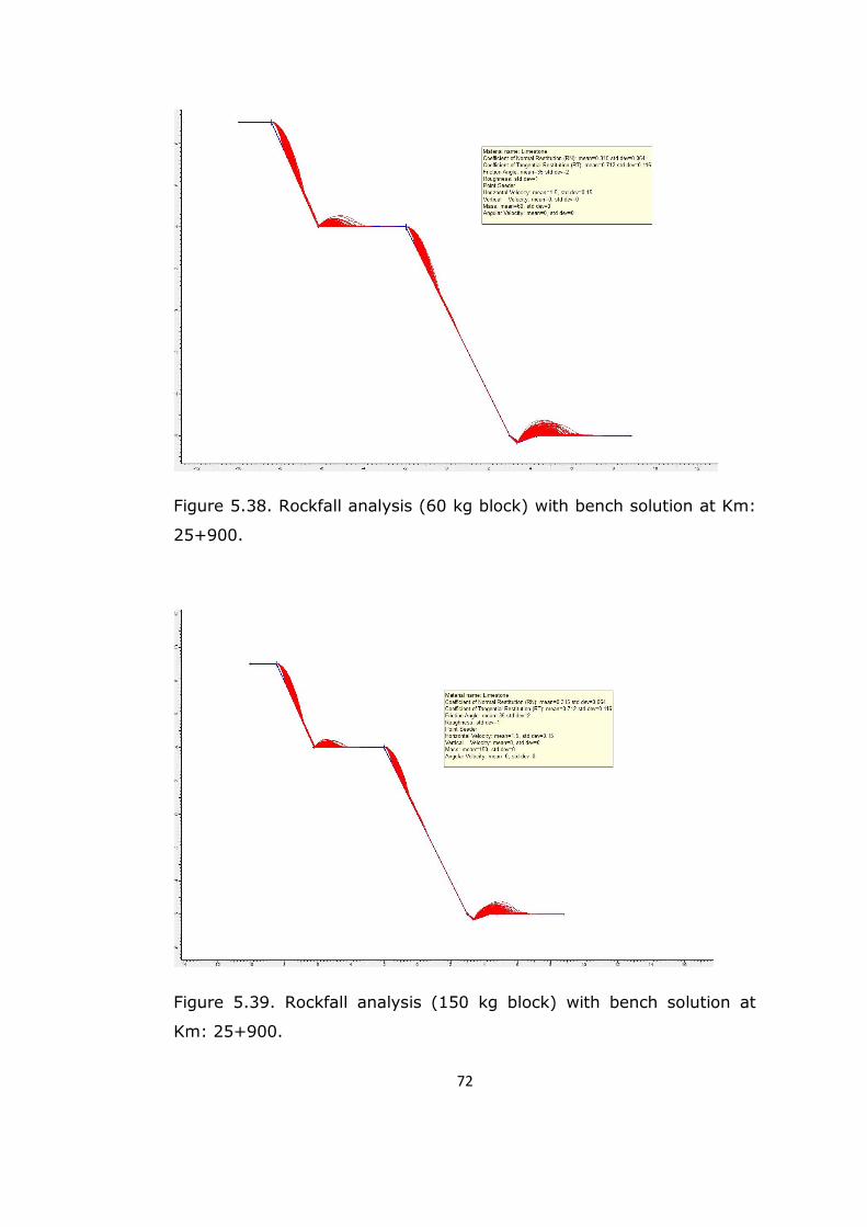
Figure 5.38. Rockfall analysis (60 kg block) with bench solution at Km:
25+900………………………………………………………………………………72
Figure 5.39. Rockfall analysis (150 kg block) with bench solution at Km:
25+900………………………………………………………………………………72
Figure 5.40. Rockfall analysis (10 kg block) with slope flattening and
barrier solution at Km: 25+900……………………………………73
Figure 5.41. Rockfall analysis (60 kg block) with slope flattening and
barrier solution at Km: 25+900………………………………………74
Figure 5.42. Rockfall analysis (150 kg block) with slope flattening and
barrier solution at Km: 25+900………………………………………74
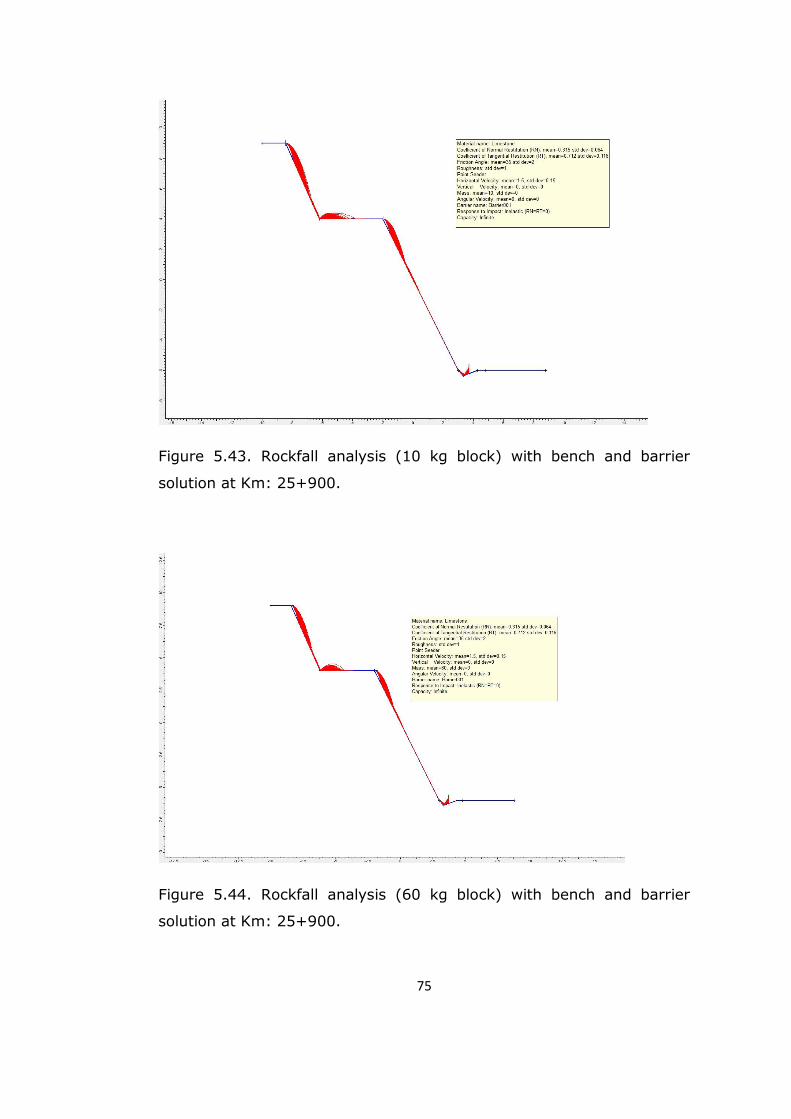
Figure 5.43. Rockfall analysis (10 kg block) with bench and barrier
solution at Km: 25+900……………………………………………………75
Figure 5.44. Rockfall analysis (60 kg block) with bench and barrier
solution at Km: 25+900……………………………………………………75
Figure 5.45. Rockfall analysis (150 kg block) with bench and barrier
solution at Km: 25+900……………………………………………………76
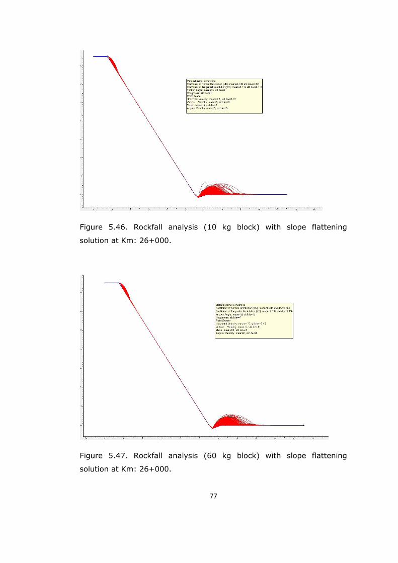
Figure 5.46. Rockfall analysis (10 kg block) with slope flattening solution
at Km: 26+000……………………………………………………………………77
xxi
Figure 5.47. Rockfall analysis (60 kg block) with slope flattening solution
at Km: 26+000……………………………………………………………………77
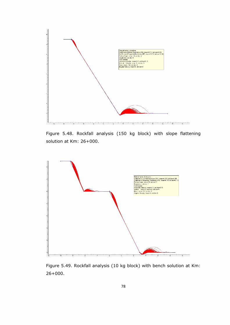
Figure 5.48. Rockfall analysis (150 kg block) with slope flattening
solution at Km: 26+000……………………………………………………78
Figure 5.49. Rockfall analysis (10 kg block) with bench solution at Km:
26+000………………………………………………………………………………78
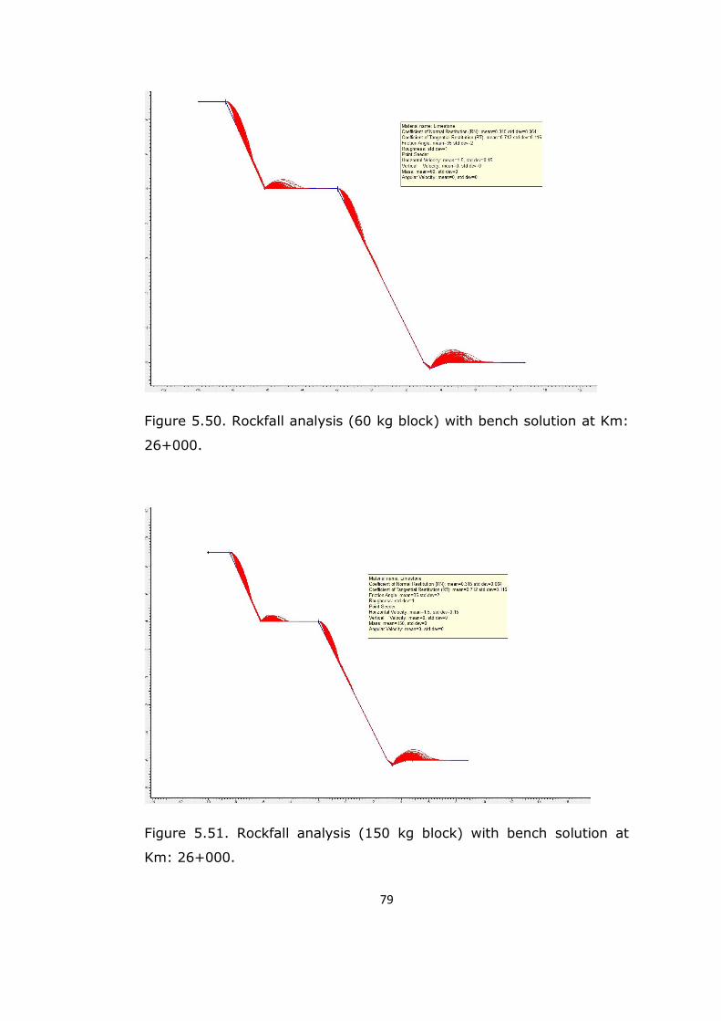
Figure 5.50. Rockfall analysis (60 kg block) with bench solution at Km:
26+000………………………………………………………………………………79
Figure 5.51. Rockfall analysis (150 kg block) with bench solution at Km:
26+000………………………………………………………………………………79
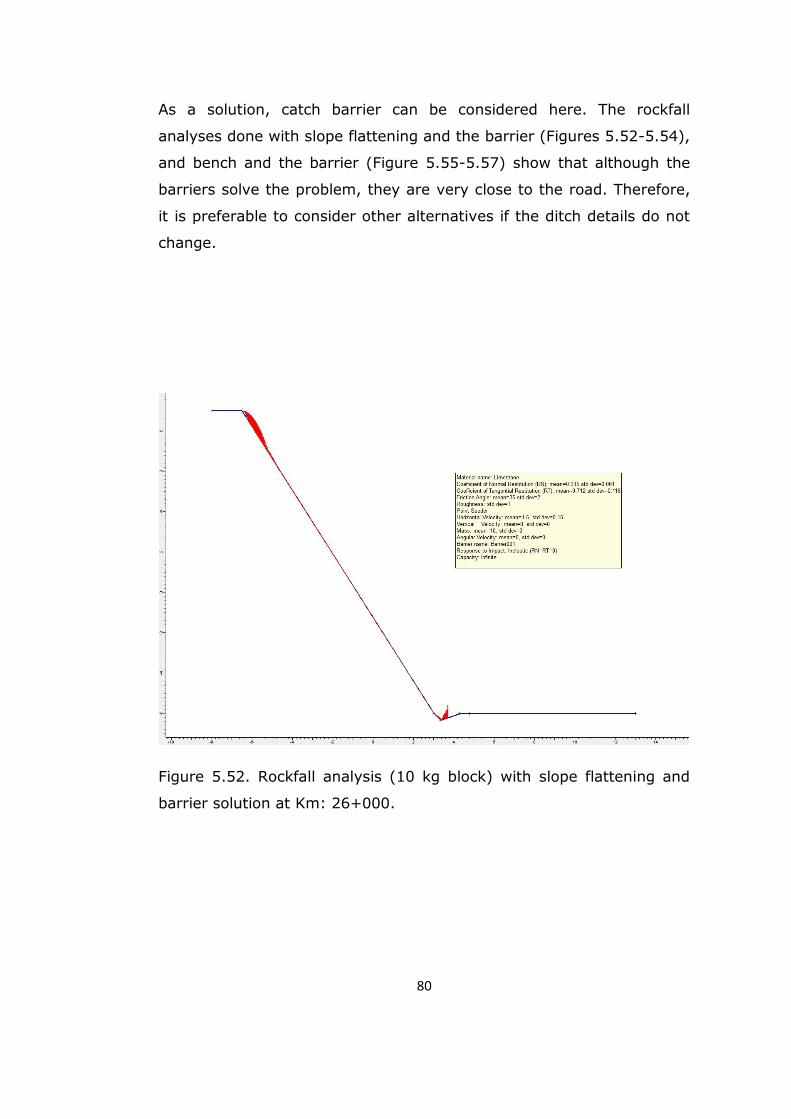
Figure 5.52. Rockfall analysis (10 kg block) with slope flattening and
barrier solution at Km: 26+000………………………………………80
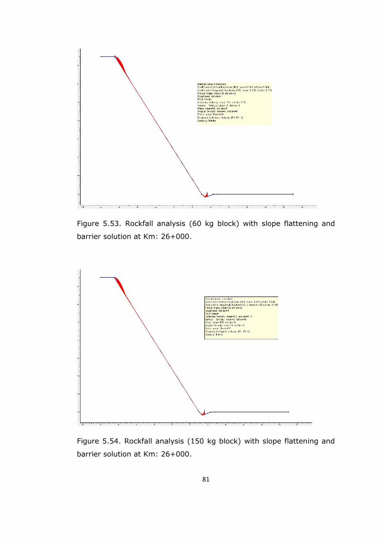
Figure 5.53. Rockfall analysis (60 kg block) with slope flattening and
barrier solution at Km: 26+000………………………………………81
Figure 5.54. Rockfall analysis (150 kg block) with slope flattening and
barrier solution at Km: 26+000………………………………………81
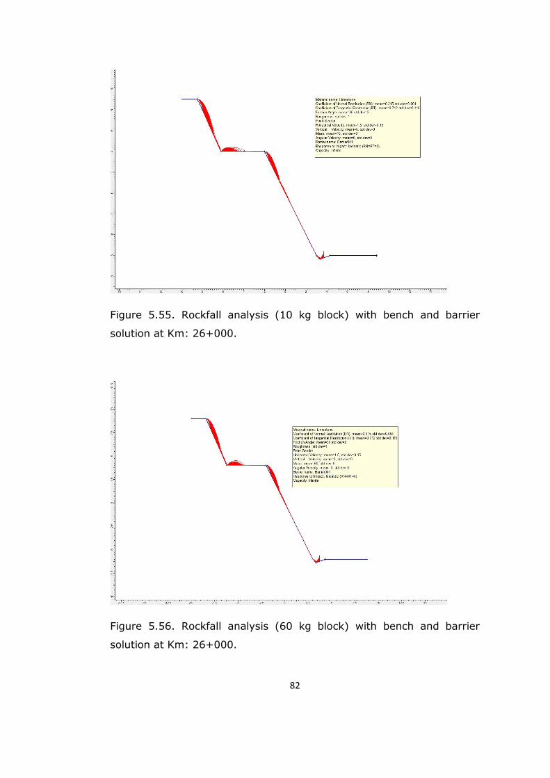
Figure 5.55. Rockfall analysis (10 kg block) with bench and barrier
solution at Km: 26+000……………………………………………………82
Figure 5.56. Rockfall analysis (60 kg block) with bench and barrier
solution at Km: 26+000……………………………………………………82
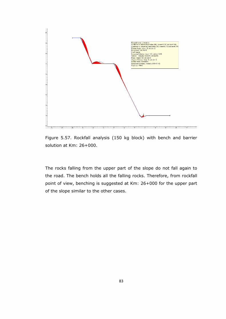
Figure 5.57. Rockfall analysis (150 kg block) with bench and barrier
solution at Km: 26+000……………………………………………………83
1
CHAPTER 1
INTRODUCTION
1.1. Purpose and Scope
Antalya-İzmir State Highway is becoming important due to increase in
traffic, especially related to tourism. However, the present road from
the Antalya-Burdur Breakaway-Korkuteli (Km: 25+500-63+500) is out
of standard and now cannot take additional traffic load. Therefore, a
new road project with widening of the existing one is initiated. The new
road will be part of the Antalya-İzmir State Highway with 2x2 lane
motorway. It has 22.00-26.00 m of platform width.
Various lithologies and several natural or cut-slopes exist along the
highway route. The field studies reveal that the section of the Antalya-
Burdur Breakaway-Korkuteli highway from Km: 25+600 to 26+000 is
located in limestone and has three slopes having slope instability
problems.
The purpose of this study is to investigate the engineering geological
properties of the limestone exposed at Km: 25+600-26+000, to assess
stability of the slopes for different mode of failures, and to suggest
necessary remedial measures that can be adopted in practice.
In order to accomplish this task, a detailed field study including
engineering description of the limestone and scan-line survey was
2
conducted. The samples taken were tested in the laboratory. The data
obtained from both the field and the laboratory were used for
kinematic, limit equilibrium and rockfall analysis.
1.2. Location and Properties of the Road
Antalya-Korkuteli State Road starts at Km: 25+578 at the north of
Thermessos National Park. At Km: 26+660, it crosses the Yeniceboğazı
Stream by a bridge and makes curves through NW. Km: 31+550,
Bayatbademleri Junction comes and it continues parallel to the Cinli
Stream through west. At Km: 38+000, it passes the Naldöken Junction,
and curves to SW at the Gölcük Alluvium Plateau. At 2 km south of the
Söğütçük Village, it curves to W again, and passes from the Canavar
Gate, and reaches the Bayat Junction. At Km: 49+600, it reaches to
Yazır Junction, and at Km: 54+450, it crosses Marzuman Stream with a
bridge and continues parallel to the stream. It leaves the present road
at Km: 55+030, turns from the S and W of Korkuteli. Finally, the road
turns to W and end at Fethiye at Km: 63+603 (Figures 1.1 and 1.2).
The properties of the project are given below:
Road Type and Class: State Road, 1st Class
Lane Number and Width: 2x2, 3.50 m
Platform Width: 22.00-26.00 m
Refuge Width: 2.00-4.00 m
Expropriation Width: 40.00-50.00 m
Sidewalk Width: 3.00 m
Bench Width: 5.00 m
3
İnceleme Alanı ve Dolayının
Uydu Görünümü
Figure 1.1. Satellite view of the study area (from Google Earth, 2010)
Beginning of
the Project
End of the
Project
Sonu
63+500
4
LEG
EN
DH
igh
wa
ys
Co
nst
ruct
ing
Hig
hw
ay
sS
tate
Ro
ad
s
Cit
y R
oa
ds
Div
ided
Roa
dsC
on
cret
e A
sph
alt
Ro
ad
s
Surf
ace
Dre
ssin
g Ro
ads
Sta
bili
zed
Ro
ad
s
Uni
mpr
oved
Roa
dR
ou
gh
ro
ad
s
Stat
e Ro
ad K
.K. N
o.C
ity
Ro
ad
K.K
. N
o.
Mou
ntai
n Pa
sses
Sta
te B
ou
nd
ary
City
Bou
ndar
yG
DH
Dis
tric
t B
ou
nd
ary
Dep
artm
ent
Boun
dary
Cit
y C
entr
e
Dis
tric
t Ce
ntre
Su
b d
istr
ict
Cen
tre
Vill
age
Loca
tion
Reg
ion
Cen
tre
Dep
artm
ent
Cent
reR
eha
bili
tati
on
Cen
tre
Refu
ge A
rea
13
th D
istr
ict A
NTA
LY
A
Fig
ure
1.2
. Location m
ap o
f th
e s
udy a
rea.
Stu
dy A
rea
Fig
ure
1.2
. Location a
nd t
ransport
ation m
ap o
f th
e s
tudy a
rea (
GD
H)
Stu
dy A
rea
5
1.3. Vegetation and Climate
The climate of Antalya is generally of Mediterranean type. It is hot and
dry in the summers and warm and wet in the winters. In the inner
parts of the region, “Cold Mid-Continental” climate is dominant.
The average temperature in the summers is between 28 and 36 °C. At
the midday, temperature gets hotter than 40 °C. In January, the
average temperature changes between 10 and 20 °C. Snow is not seen
in the city. Frost is almost never seen. When the weather is not rainy,
it is clear and sunny. In Antalya, where the average relative humidity
is % 64, the average temperature of sea water is 17.6 °C in January,
18.0 °C in April, 27.7 °C in August and 24.5 °C in October. On the
coast of Antalya, summertime is long and hot. Even in winters, the
temperature is cool to warm. While the rain is unavailable in summer,
downpour of rain is frequent in December and January, but rare during
the months of fall and spring. Barely 40-50 days of the year are
overcast and rainy. Antalya is one of the rare regions which are
available for tourism with average 300 sunny days during the year and
the yearly average temperature of 18.7 °C. It is possible to have a
swim at least for the nine months of the year (Antalya Municipality,
2007a).
Lemur, which is suitable for extreme summer draughts and stays green
during the wintertime, is dominant from the shore to the heights of
500-600 m. Ryegrass, arbutus, sandalwood, wild strawberries and
oleander are common among lemur which has a maximum height of 3-
5 m. Between the altitude of 600-1200 m, there appears the mixed or
hillside forests where Pinus brutia and oak are widespread. Oak groves
are seen between Pinus brutia, and on higher altitudes Aleppo pine and
black pine begins to appear. Between the altitudes of 1200-2100 m
there is a zone of high forests which consists of cedar, fir, scotch pine,
6
beech, and various juniper types. Especially in the Western Taurus,
there are wholesome cedar forests. Above the altitude of 2000 m
coniferous trees become sparse and short. This zone ends between
2100-2300 m, and passes through high hayricks, so called the alpine
meadows, which consists of colorful flowers and does not run dry
during summertime. In the high plains of Teke Plateau, steppe plants
have grown out due to the destruction of oak trees. In the forests of
Antalya extending to 946.466 hectares, there are types of herb and
tree like fir, oak, ashen, elm, arbutus, sycamore, wild pear, linden, wild
and inoculated olive, kermes oak, dyer's oak, sandalwood, gumwood,
myrtle, Melia azaderach, daphne, Phllyrea, agnus-castus, oleander,
carob, hop-hornbeam, heather, spruce, dyer's rocket, genista, thyme,
popper, spurge, thorny myrtle, musk thistle, dead nettle, sage, saffron,
Kanadisches Berufkraut, Sarcopoterium spinosum L., Asphodelus,
asparagus, chrysanthemum (Antalya Municipality, 2007b).
The area of Korkuteli district is 2471 km2. Its altitude from the
shoreline is 1020 m, and its climate is Mediterranean with the ratio of
¼, and Lake District type continental with the ratio of ¾. The four
seasons are apparent in the district and the average temperature is -5
°C in wintertime and 25 °C in summertime (Antalya Agriculture, 2007).
There is a terrain structure consisting of plains and hills at the back
side of the Beydağları facing towards Mediterranean. Naturally, the
slopes and feet of Beydağları is covered with pine groves, shrubbery
and forests; on the other side plains are used for agricultural means. In
the district 101.465 hectares are agricultural fields, 5800 hectares are
lawn and pasture, 100.339 hectares are forests and shrubbery, 351
hectares are water surface, and 40.313 hectares are residential and
non-agricultural areas. 116 hectares of the agricultural field is located
within the area of the forests (Antalya Agriculture, 2007).
7
1.4. Methods of Study
The study has been carried out in several stages. The first stage was to
perform a detailed literature survey. In this part, previous studies
completed around the study area have been obtained and the
fundamental theories related to engineering geology and slope
instability have been searched.
Secondly, the field studies were carried out. It includes field description
of the engineering geological properties of the limestone, performing
scan-line surveys at three cut slopes and obtaining nine oriented
samples with discontinuities.
Thirdly, laboratory studies were performed on the rock samples
obtained from the field. Unit weight and uniaxial compressive strength
of the limestone, and shear strength parameters (cohesion and internal
friction angle) of the discontinuities are measured in accordance with
ISRM (1981).
Then, the discontinuity orientation data were analyzed with DIPS
(2004) software to assess the dominant discontinuity sets. Limit
equilibrium analyses for three cut slopes were performed with SLIDE
(2004) software for different slope geometries and without/with
remedial measures. Rockfall analyses were performed to assess the
possibility if a detached rock for different weights reaches the highway
to endanger the highway traffic.
Finally, all of these analyses were evaluated together to recommend
possible remedial measures for the Km: 25+600-26+000 section of the
planned road.
8
1.5. Previous Studies
Although many studies are done around the Antalya Region, there are
only few studies in this particular Antalya-Korkuteli region. The first
geological study in the Korkuteli Road was done by Colin (1962). He
studied in a very wide region around Fethiye-Antalya-Kaş and Finike,
and the defined the Beydağları formation and the Alakırçay Group
which crop out along the Antalya-İzmir Satate Highway route.
Şenel et al. (1994) studied this region and gave detailed explanation
about the Beydağları formation. They have revealed the contact
information for this unit. This work was related to the study area in
only one unit.
Şenel (1997) gave a detailed explanation about almost all of the units
that can be seen along the planned road. In this study, the Beydağları
formation was explained in detail. He mentioned the Söbütepe
formation (Upper Paleocene-Lower Eocene) which outcrops at the road
and said the lower boundary of this unit is discordant. In this study,
Antalya nappes were also given in detail. In this part of the study,
some details of Tilkideliğitepe formation, Yeniceboğazıdere formation
and Limestone Unit are given in details. He also described the Alakırçay
nappe and the Alakırçay Group. All of these units outcrop in the
planned road. However, the Limestone Unit of Şenel (1997) is seen at
the three cut slopes that are studied in this thesis.
FORM Jeoteknik (2008) carried out a geological and geotechnical study
in the proposed Antalya-Burdur Breakaway-Korkuteli State Road Km:
25+500-63+500. They prepared geological and engineering geological
maps, and the geological profile for the area. Beril Drilling Co drilled
many boreholes and trial pits along the planned road in 2006, 2 of
which are very close to the thesis area. FORM Jeoteknik (2008)
evaluated the data obtained from the field and laboratory and carried
out some kinematic and stability analysis of earth and cut slopes.
Geological and engineering geological assessment of the planned road
9
for the cut-slopes and the embankments were also done. The author of
this thesis was also involved at all stages of the project for FORM-Beril
Co during the geotechnical investigations.
There are other studies not directly related to the study area but
related to the region. Pisoni (1967) mentioned about the Kaş limestone
(Maastrichtian-Lutetian), Pınarbaşı formation (Lower Miocene) and
Felenkdağı conglomerate (Lower Miocene). Poisson and Poignant
(1974) studied the Katrandağı formation (Cenomanian). They also
studied on the Karabayır formation (Miocene and Cretaceous-
Paleogene) around Korkuteli.
10
CHAPTER 2
GEOLOGY AND SEISMICITY OF THE STUDY AREA
2.1. Geology of the Study Area
Although various lithological units are exposed along the Antalya-
Burdur Breakaway-Korkuteli highway (Figure 2.1), the Limestone unit
belonging to Çataltepe Nappe is the main lithological unit of the
highway segment studied in this thesis.
The Çataltepe Nappe consists of three formations, namely
Tilkideliğitepe formation (TRt), Yeniceboğazıdere Formation (JKy), and
the Limestone Unit (JKyk).
The Tilkideliğitepe formation (TRt) contains massive, partly thin-
medium-thick layered, greenish gray to light brown marls, and
limestone lenses and blocks rich in macro fossils. The lower boundary
of this formation is tectonic and the upper boundary is concordant with
the Yeniceboğazıdere formation. The thickness of this unit is about 100
meters. The formation has been deposited in shelf environment. The
age of the formation is Norian based on its fossil content (Şenel, 1977).
11
Fig
ure
2.1
Geolo
gic
al m
ap o
f th
e s
tudy a
rea (
modifie
d fro
m M
TA,
2004)
12
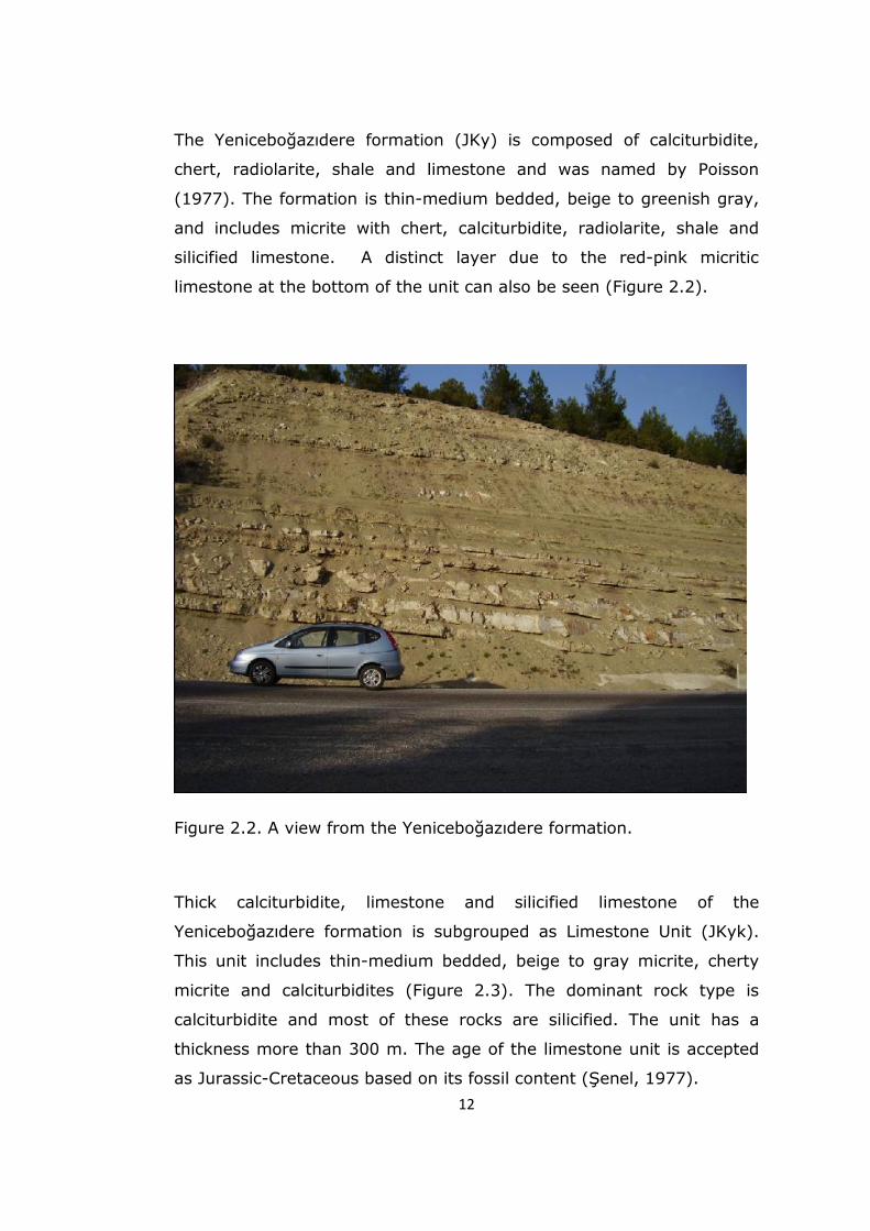
The Yeniceboğazıdere formation (JKy) is composed of calciturbidite,
chert, radiolarite, shale and limestone and was named by Poisson
(1977). The formation is thin-medium bedded, beige to greenish gray,
and includes micrite with chert, calciturbidite, radiolarite, shale and
silicified limestone. A distinct layer due to the red-pink micritic
limestone at the bottom of the unit can also be seen (Figure 2.2).
Figure 2.2. A view from the Yeniceboğazıdere formation.
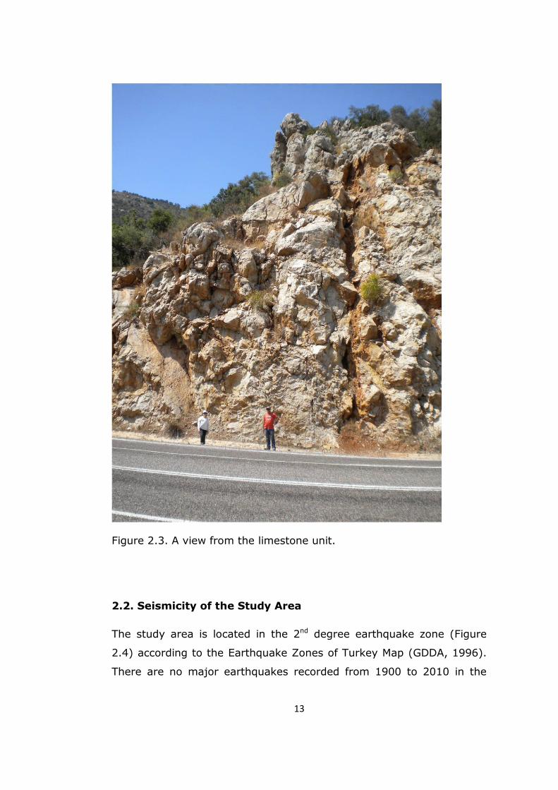
Thick calciturbidite, limestone and silicified limestone of the
Yeniceboğazıdere formation is subgrouped as Limestone Unit (JKyk).
This unit includes thin-medium bedded, beige to gray micrite, cherty
micrite and calciturbidites (Figure 2.3). The dominant rock type is
calciturbidite and most of these rocks are silicified. The unit has a
thickness more than 300 m. The age of the limestone unit is accepted
as Jurassic-Cretaceous based on its fossil content (Şenel, 1977).
13
Figure 2.3. A view from the limestone unit.
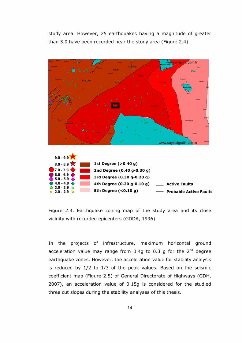
2.2. Seismicity of the Study Area
The study area is located in the 2nd degree earthquake zone (Figure
2.4) according to the Earthquake Zones of Turkey Map (GDDA, 1996).
There are no major earthquakes recorded from 1900 to 2010 in the
14
study area. However, 25 earthquakes having a magnitude of greater
than 3.0 have been recorded near the study area (Figure 2.4)
www.e-harita.com.tr
www.sayisalgrafik.com.tr
Suğlu Gölü
Girdev Gölü
Karataş Gölü
Akgöl
Kuru Göl
Koca Göl
Beyşehir Gölü
Kovada Gölü
Acıpayam
Ahırlı
Akseki
Aksu
Alanya
Antalya
Beyşehir
Bozkurt
Bucak
Denizli
Derebucak
ElmalıFethiye
Finike
Gazipaşa
Gündoğmuş
Honaz
Kale
Kaş
Kemer
Keçiborlu
Korkuteli
Kumluca
Manavgat
Meram
Sarıveliler
Serinhisar
Seydişehir
Sütçüler
Tavas
Taşkent
Çeltikçi
Çumra
İbradı
Akören
Bozkır
Burdur
Hadım
Isparta
Figure 2.4. Earthquake zoning map of the study area and its close
vicinity with recorded epicenters (GDDA, 1996).
In the projects of infrastructure, maximum horizontal ground
acceleration value may range from 0.4g to 0.3 g for the 2nd degree
earthquake zones. However, the acceleration value for stability analysis
is reduced by 1/2 to 1/3 of the peak values. Based on the seismic
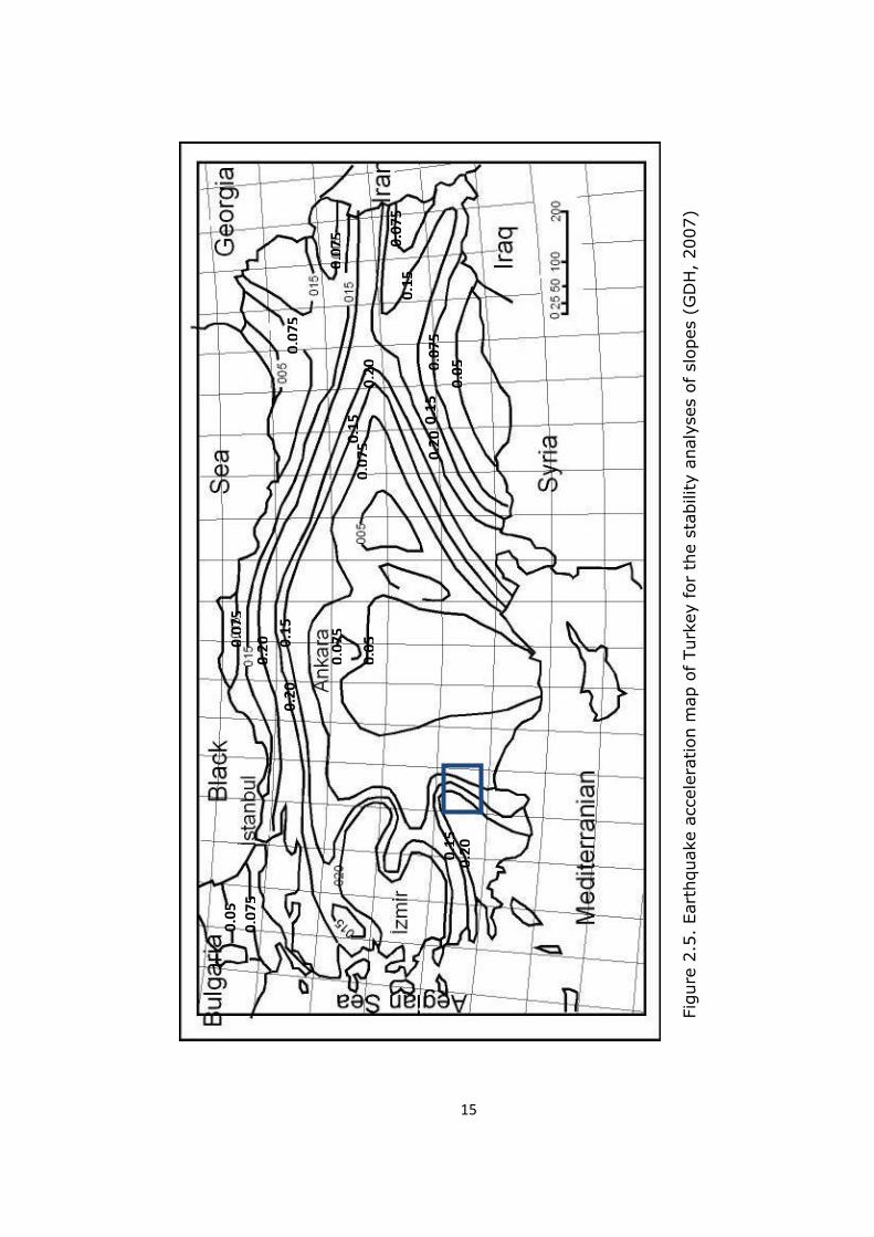
coefficient map (Figure 2.5) of General Directorate of Highways (GDH,
2007), an acceleration value of 0.15g is considered for the studied
three cut slopes during the stability analyses of this thesis.
0.2
0
0.1
5
0.0
75
0
.05
0.0
75
0
.15
0
.20
0.2
0 0
.15
0
.07
5
0.0
5
0.1
5
0.0
75
0.2
0
0.1
5
0.2
0
0.0
75
0.0
75
0.0
75
0.0
75
0.0
5
1st Degree (>0.40 g)
2nd Degree (0.40 g-0.30 g)
3rd Degree (0.30 g-0.20 g)
4th Degree (0.20 g-0.10 g)
5th Degree (<0.10 g)
Active Faults
Probable Active Faults
15
Fig
ure
2.5
. Eart
hquake a
ccele
ration m
ap o
f Turk
ey for
the s
tability a
naly
ses o
f slo
pes (
GD
H,
2007)
0.2
0
0.1
5
0.0
75
0
.05
0.0
75
0
.15
0
.20
0.2
0 0
.15
0
.07
5
0.0
5
0.1
5
0.0
75
0.2
0
0.1
5
0.2
0
0.0
75
0.0
75
0.0
75
0.0
75
0.0
5
16
CHAPTER 3
ENGINEERING GEOLOGICAL PROPERTIES OF THE LIMESTONE
EXPOSED AT KM: 25+600-26+000
In this chapter, the engineering geological properties of the limestone
belonging to the Çataltepe nappe at Km: 25+600-26+000 section of
the highway will be given. At three sections of the highway where slope
instability problems exist, field descriptions (material and mass) of the
limestone were done. Scanline-surveys (each for a length of at least 30
m) along natural rock exposures were performed in accordance with
Priest (1993) at suitable locations near the highway. The directional
data obtained from the surveys were evaluated by using DIPS (2004)
software of Rocscience. The data are plotted through Schmidt net using
the lower hemisphere projection. Diagrams for pole and contour plots,
rose diagram and dominant discontinuity sets are determined for this
part of the road in three cut slopes.
Twelve oriented samples were taken from the field for laboratory
testing. The laboratory tests were conducted at the Department of
Geological and Mining Engineering of METU). Unit weight and uniaxial
compressive strength of the limestone, and shear strength parameters
(cohesion and internal friction angle) along the discontinuities were
determined following the procedures given in ISRM (1981).
17
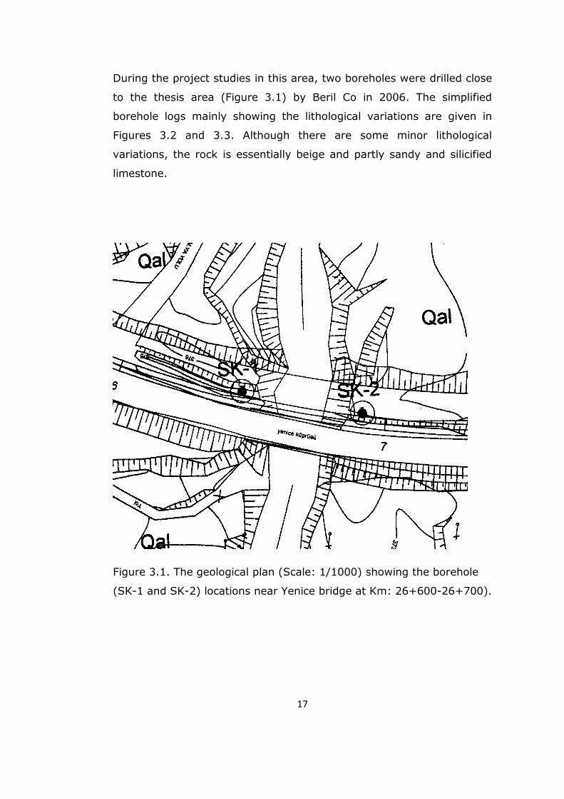
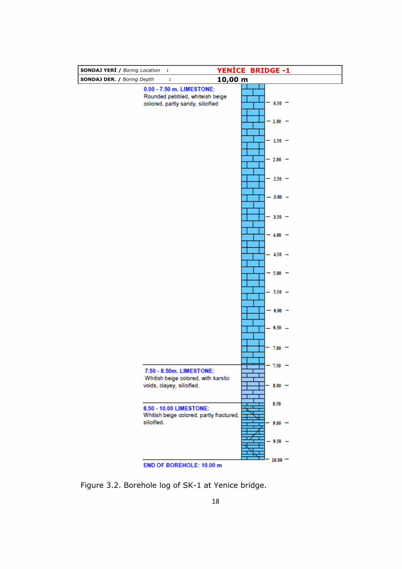
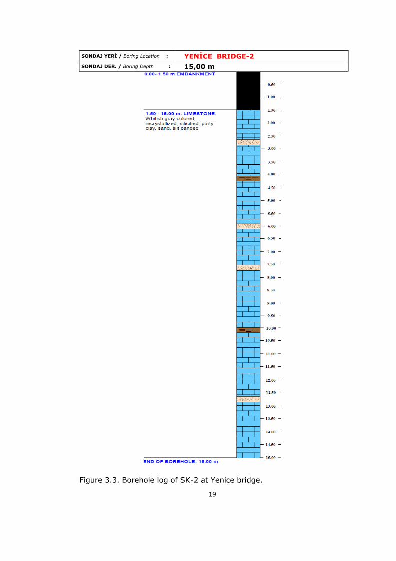
During the project studies in this area, two boreholes were drilled close
to the thesis area (Figure 3.1) by Beril Co in 2006. The simplified
borehole logs mainly showing the lithological variations are given in
Figures 3.2 and 3.3. Although there are some minor lithological
variations, the rock is essentially beige and partly sandy and silicified
limestone.
Figure 3.1. The geological plan (Scale: 1/1000) showing the borehole
(SK-1 and SK-2) locations near Yenice bridge at Km: 26+600-26+700).
18
Figure 3.2. Borehole log of SK-1 at Yenice bridge.
SONDAJ YERİ / Boring Location : YENİCE BRIDGE -1
SONDAJ DER. / Boring Depth : 10,00 m
19
SONDAJ YERİ / Boring Location : YENİCE BRIDGE-2
SONDAJ DER. / Boring Depth : 15,00 m
Figure 3.3. Borehole log of SK-2 at Yenice bridge.
20
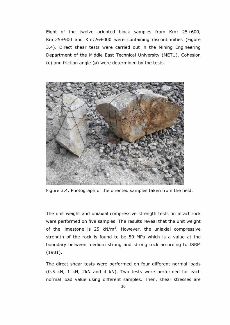
Eight of the twelve oriented block samples from Km: 25+600,
Km:25+900 and Km:26+000 were containing discontinuities (Figure
3.4). Direct shear tests were carried out in the Mining Engineering
Department of the Middle East Technical University (METU). Cohesion
(c) and friction angle (ø) were determined by the tests.
Figure 3.4. Photograph of the oriented samples taken from the field.
The unit weight and uniaxial compressive strength tests on intact rock
were performed on five samples. The results reveal that the unit weight
of the limestone is 25 kN/m3. However, the uniaxial compressive
strength of the rock is found to be 50 MPa which is a value at the
boundary between medium strong and strong rock according to ISRM
(1981).
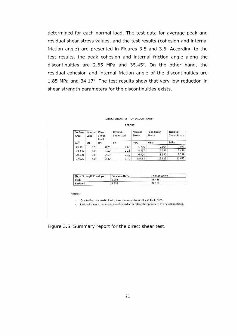
The direct shear tests were performed on four different normal loads
(0.5 kN, 1 kN, 2kN and 4 kN). Two tests were performed for each
normal load value using different samples. Then, shear stresses are
21
determined for each normal load. The test data for average peak and
residual shear stress values, and the test results (cohesion and internal
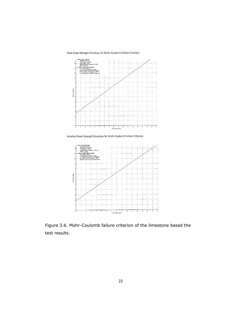
friction angle) are presented in Figures 3.5 and 3.6. According to the
test results, the peak cohesion and internal friction angle along the
discontinuities are 2.65 MPa and 35.45o. On the other hand, the
residual cohesion and internal friction angle of the discontinuities are
1.85 MPa and 34.17o. The test results show that very low reduction in
shear strength parameters for the discontinuities exists.
Figure 3.5. Summary report for the direct shear test.
22
Figure 3.6. Mohr-Coulomb failure criterion of the limestone based the
test results.
23
3.1. Engineering Geological Properties of the Limestone at Km:
25+600
The limestone at this locality is beige to gray, fine grained (micritic),
fossiliferous, and highly jointed (Figure 3.7). Fifty six discontinuity
measurements were taken during the scan-line survey carried out for a
length of nearly 30 meters. The joints and bedding plane constitute the
major discontinuities at this location.
Figure 3.7. A view from the limestone facing north at Km: 25+600.
The discontinuities generally have close to wide (60 mm-1000 mm)
spacing, tight to partly open (0.1 mm-0.5 mm) aperture, planar rough
to undulating rough discontinuity surfaces, slightly weathered mainly in
24
the form of discoloration along discontinuity surfaces although some
karstic cavities exists near the surface, medium strong and strong. The
discontinuities have practically no infill material except upper 1 m. On
the other hand, the discontinuities are locally filled by secondary
calcite. Most of the discontinuities (bedding planes and joints) have
high persistence mainly greater than 10 m, but one of the joint set is
bed confined. No groundwater seepage was encountered at this
location.
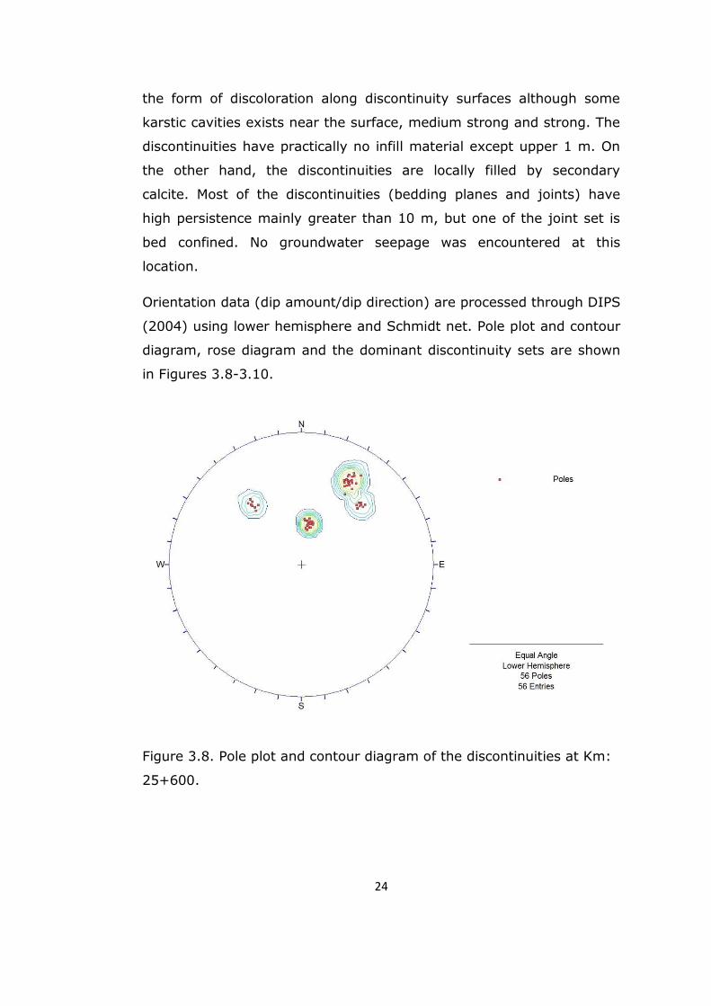
Orientation data (dip amount/dip direction) are processed through DIPS
(2004) using lower hemisphere and Schmidt net. Pole plot and contour
diagram, rose diagram and the dominant discontinuity sets are shown
in Figures 3.8-3.10.
Figure 3.8. Pole plot and contour diagram of the discontinuities at Km:
25+600.
25
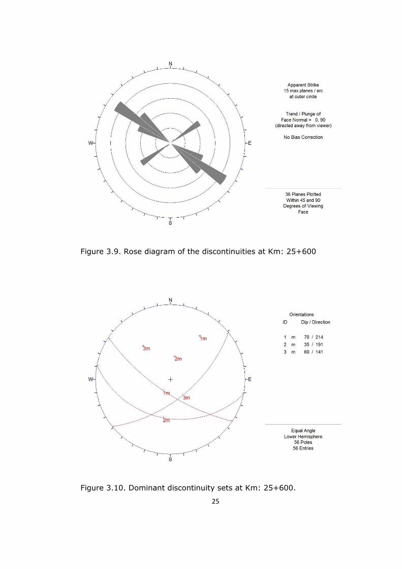
Figure 3.9. Rose diagram of the discontinuities at Km: 25+600
Figure 3.10. Dominant discontinuity sets at Km: 25+600.
26
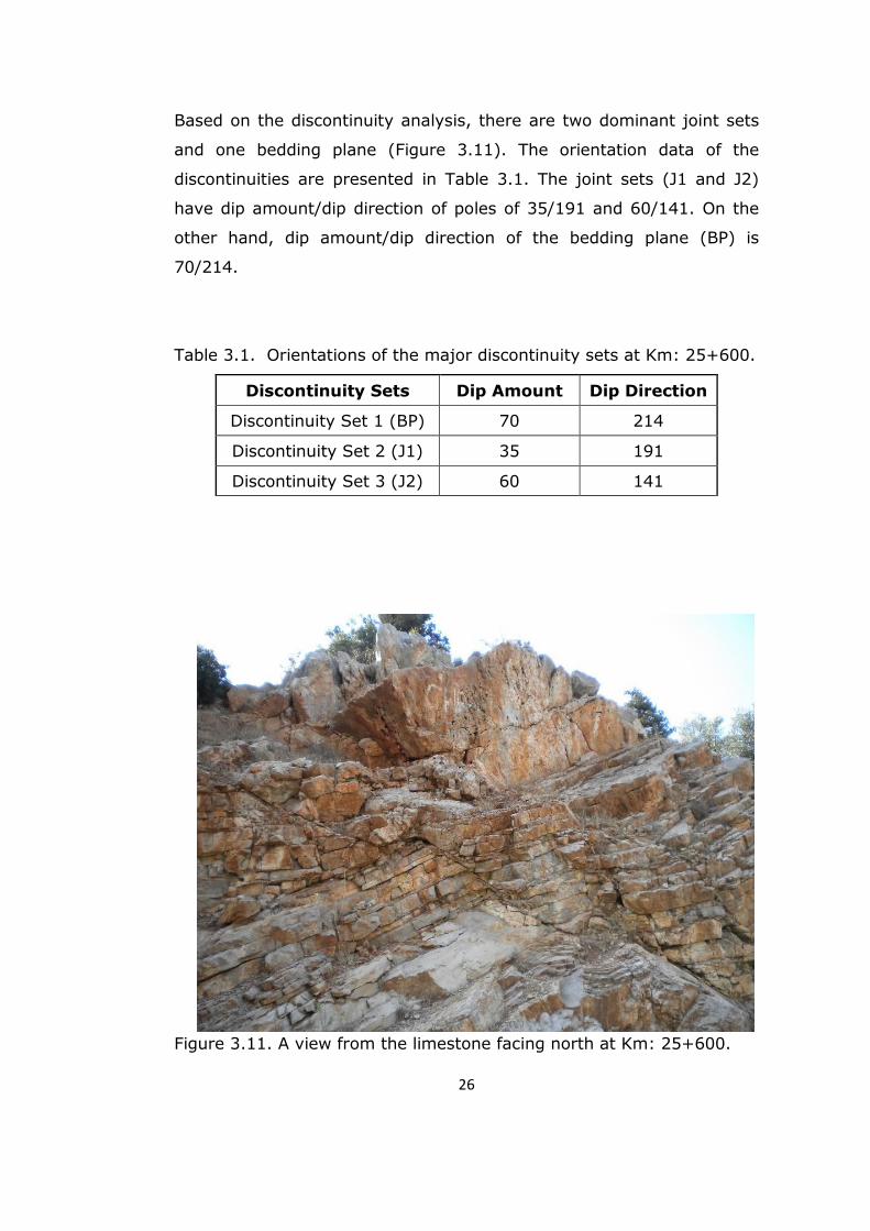
Based on the discontinuity analysis, there are two dominant joint sets
and one bedding plane (Figure 3.11). The orientation data of the
discontinuities are presented in Table 3.1. The joint sets (J1 and J2)
have dip amount/dip direction of poles of 35/191 and 60/141. On the
other hand, dip amount/dip direction of the bedding plane (BP) is
70/214.
Table 3.1. Orientations of the major discontinuity sets at Km: 25+600.
Discontinuity Sets Dip Amount Dip Direction
Discontinuity Set 1 (BP) 70 214
Discontinuity Set 2 (J1) 35 191
Discontinuity Set 3 (J2) 60 141
Figure 3.11. A view from the limestone facing north at Km: 25+600.
27
3.2. Engineering Geological Properties of Limestone at Km:
25+900
The limestone at this locality is very similar to the one observed at
Km:25+600. The rock is beige to gray, fine grained, and highly jointed
(Figure 3.12). One hundred fourty eight discontinuity measurements
were taken during the scan-line survey carried out for a length of
nearly 30 meters. The joints and bedding plane constitute the major
discontinuities at this location.
Figure 3.12. A view from the limestone facing north at Km: 25+900.
The discontinuities generally have close to wide (60 mm-1000 mm)
spacing, tight to partly open (0.1 mm-0.5 mm) aperture, planar rough
to undulating rough discontinuity surfaces, slightly weathered mainly in
28
the form of discoloration along discontinuity surfaces although some
karstic cavities exists near the surface, medium strong and strong. The
discontinuities have practically no infill material except upper 0.5 m. On
the other hand, the discontinuities are locally filled by secondary
calcite. Most of the discontinuities (bedding planes and joints) have
high persistence mainly greater than 10 m. However, one of the joint
set is bed confined which has very low (0.3-<1m) persistence.
Groundwater seepage was not seen during the field study around this
cut slope.
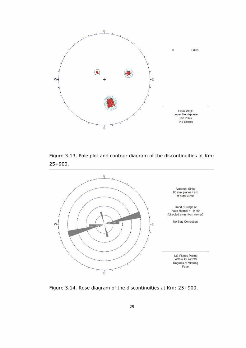
Orientation data (dip amount/dip direction) are evaluated by DIPS
(2004) software using lower hemisphere and Schmidt net. Pole plot
and contour diagram, rose diagram and the dominant discontinuity sets
are shown in Figures 3.13-3.15.
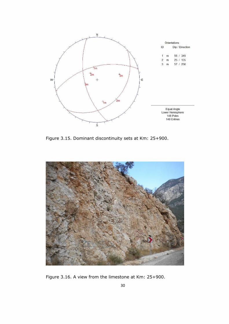
Based on the discontinuity analysis, there are two joint sets and one
bedding plane at this location (Figures 3.15 and 3.16). The orientation
data of the discontinuities are presented in Table 3.2. The joint sets
have dip amount/dip direction of 25/135 and 57/256. On the other
hand, dip amount/dip direction of the bedding plane is 55/345.
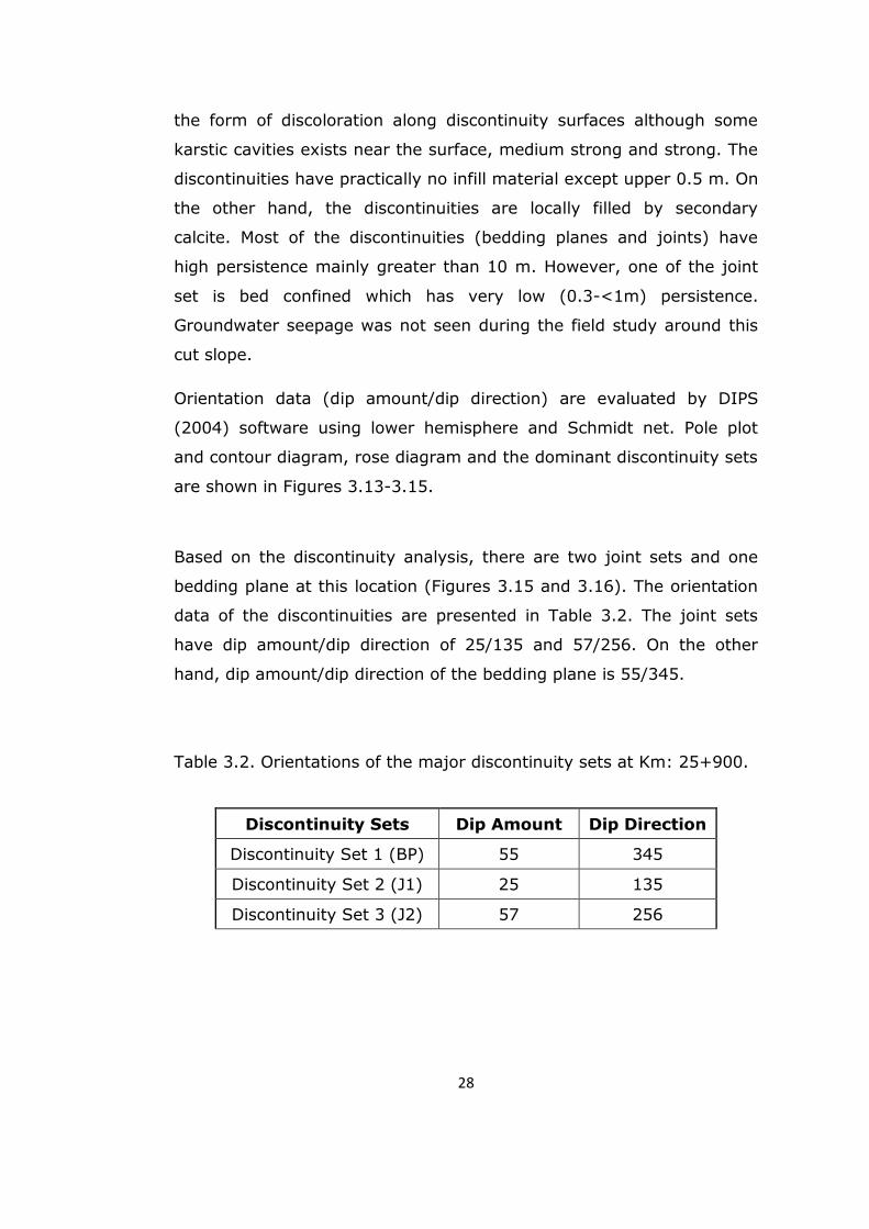
Table 3.2. Orientations of the major discontinuity sets at Km: 25+900.
Discontinuity Sets Dip Amount Dip Direction
Discontinuity Set 1 (BP) 55 345
Discontinuity Set 2 (J1) 25 135
Discontinuity Set 3 (J2) 57 256
29
Figure 3.13. Pole plot and contour diagram of the discontinuities at Km:
25+900.
Figure 3.14. Rose diagram of the discontinuities at Km: 25+900.
30
Figure 3.15. Dominant discontinuity sets at Km: 25+900.
Figure 3.16. A view from the limestone at Km: 25+900.
31
3.3. Engineering Geological Properties of Limestone at Km:
26+000
The limestone at this locality is also very similar to the one observed at
Km:25+600 and 25+900. The rock is beige to gray, fine grained, and
highly jointed (Figure 3.17). Seventy six discontinuity measurements
were taken during the scan-line survey carried out for a length of
nearly 30 meters. Similar to other two locations, the joints and bedding
plane constitute the major discontinuities at this location.
Figure 3.17. A view from the limestone facing north at Km: 26+000.
The discontinuities have close to wide (60 mm-1000 mm) spacing, tight
to partly open (0.1 mm-0.5 mm) aperture, planar rough to undulating
rough discontinuity surfaces. The weathering is dominant only near the
32
surface. It is slightly weathered mainly in the form of discoloration
along discontinuity surfaces. The rock is medium strong and strong.
Except local calcite infilling, the discontinuities have practically no infill
material. Most of the discontinuities (bedding planes and joints) have
high persistence mainly greater than 10 m. However, one of the joint
set is bed confined which has very low (0.3 - <1m) persistence.
Groundwater seepage was not detected at this locality.
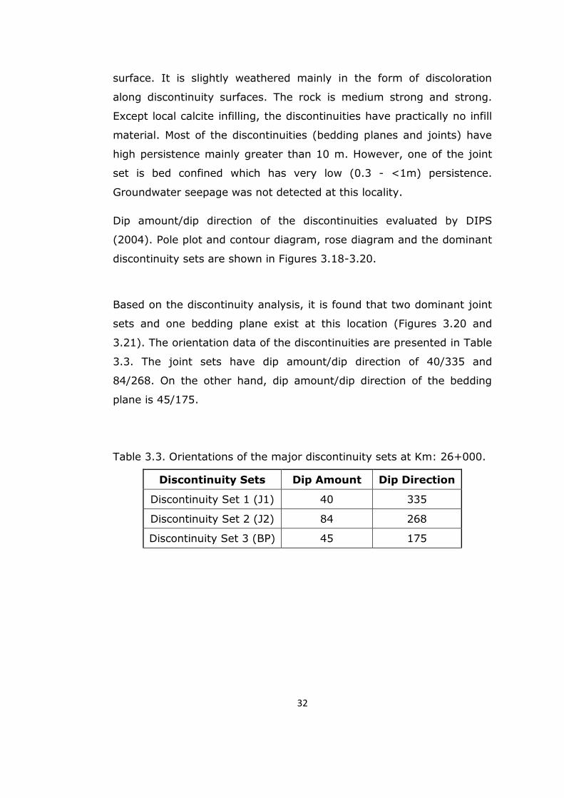
Dip amount/dip direction of the discontinuities evaluated by DIPS
(2004). Pole plot and contour diagram, rose diagram and the dominant
discontinuity sets are shown in Figures 3.18-3.20.
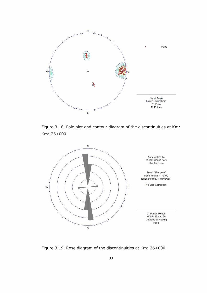
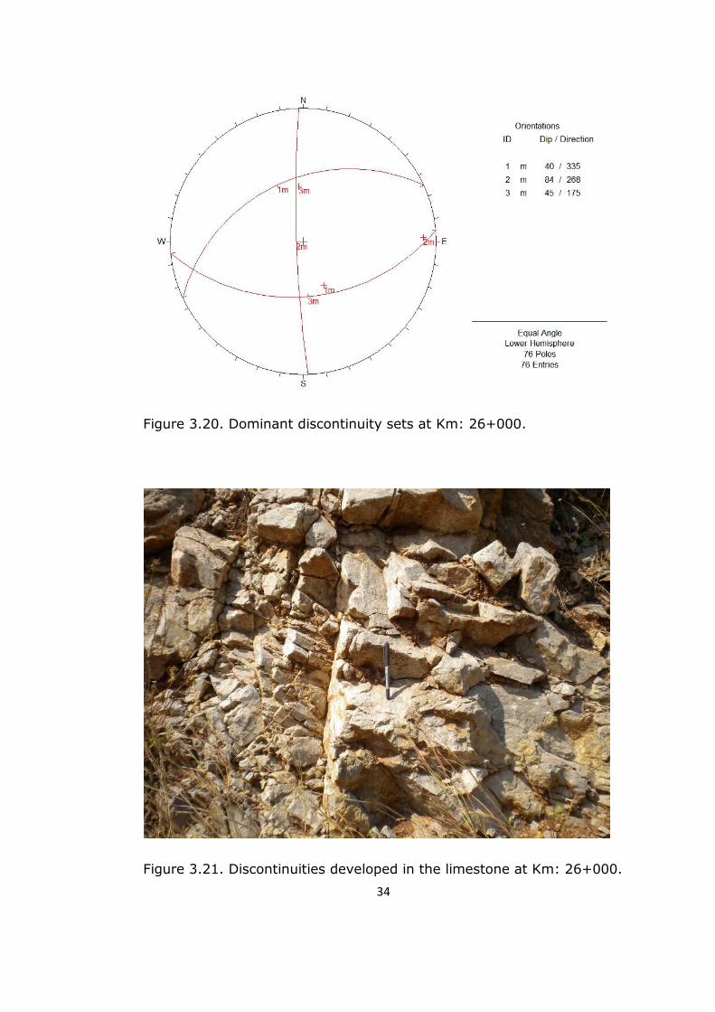
Based on the discontinuity analysis, it is found that two dominant joint
sets and one bedding plane exist at this location (Figures 3.20 and
3.21). The orientation data of the discontinuities are presented in Table
3.3. The joint sets have dip amount/dip direction of 40/335 and
84/268. On the other hand, dip amount/dip direction of the bedding
plane is 45/175.
Table 3.3. Orientations of the major discontinuity sets at Km: 26+000.
Discontinuity Sets Dip Amount Dip Direction
Discontinuity Set 1 (J1) 40 335
Discontinuity Set 2 (J2) 84 268
Discontinuity Set 3 (BP) 45 175
33
Figure 3.18. Pole plot and contour diagram of the discontinuities at Km:
Km: 26+000.
Figure 3.19. Rose diagram of the discontinuities at Km: 26+000.
34
Figure 3.20. Dominant discontinuity sets at Km: 26+000.
Figure 3.21. Discontinuities developed in the limestone at Km: 26+000.
35
CHAPTER 4
KINEMATIC ANALYSES OF THE CUT SLOPES
In this chapter, kinematic analyses of the cut slopes for Km: 25+600 -
26+000 part of the road are given. The kinematic analyses are carried
out according to the procedure described in Hoek and Bray (1981) and
Turner and Schuster (1996). The kinematic analyses are done for
planar, wedge and toppling failures, separately. For the friction angle,
35° found from the direct shear tests is used.
4.1. Kinematic Analysis of the Cut Slope at Km: 25+600
At this location, two joint sets and a bedding plane form the main
discontinuities (Figure 4.1). The kinematic analysis for planar failure
performed at Km: 25+600 shows that except one joint set, no plane
failure is expected. Nevertheless, the poles of this problematic joint set
partly fall within the daylight envelope. Since the difference of the
strikes between the slope (64/240) and the discontinuity (35/191) is
more than 20°, no planar failure is expected at this location (Figure
4.2). According to the kinematic analysis for wedge and toppling
failures (Figures 4.3 and 4.4), the cut slope is stable for both cases.
36
Figure 4.1. Photograph showing main discontinuities developed in the
limestone at Km: 25+600.
Figure 4.2. Kinematic analysis of the cut slope for planar failure at Km:
25+600.
37
Figure 4.3. Kinematic analysis of the cut slope for wedge failure at Km:
25+600.
Figure 4.4. Kinematic analysis of the cut slope for toppling failure at
Km: 25+600.
38
As a summary, according to the kinematic analyses carried out, this
part of the cut slope does not have any planar, wedge or toppling
failures. Therefore, the limit equilibrium analysis which will be
discussed in Chapter 5 of this thesis is not performed for this part of
the study area.
4.2. Kinematic Analysis of the Cut Slope at Km: 25+900
Two joint sets and a bedding plane also form the main discontinuities
at Km: 25+900 (Figure 4.5). The slope amount and its direction for the
cut slope at this location is 64/250. The kinematic analysis for plane
failure performed at Km: 25+900 shows that the poles of one joint set
(57/256) falls within the daylight envelope. Therefore, planar failure
controlled by the joint is likely to occur at this location (Figure 4.6). In
order to eliminate this problem, a slope flattening of 10° may be
recommended (Figure 4.7).
Figure 4.5. Photograph showing main discontinuities developed in the
limestone at Km: 25+900.
39
Figure 4.6. Kinematic analysis of the cut slope for planar failure at Km:
25+900.
Figure 4.7. Elimination of the planar failure kinematically by flattening
of the slope at Km: 25+900.
40
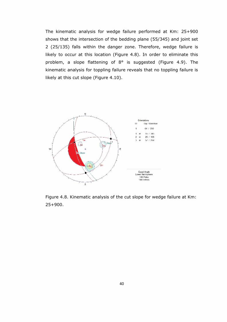
The kinematic analysis for wedge failure performed at Km: 25+900
shows that the intersection of the bedding plane (55/345) and joint set
2 (25/135) falls within the danger zone. Therefore, wedge failure is
likely to occur at this location (Figure 4.8). In order to eliminate this
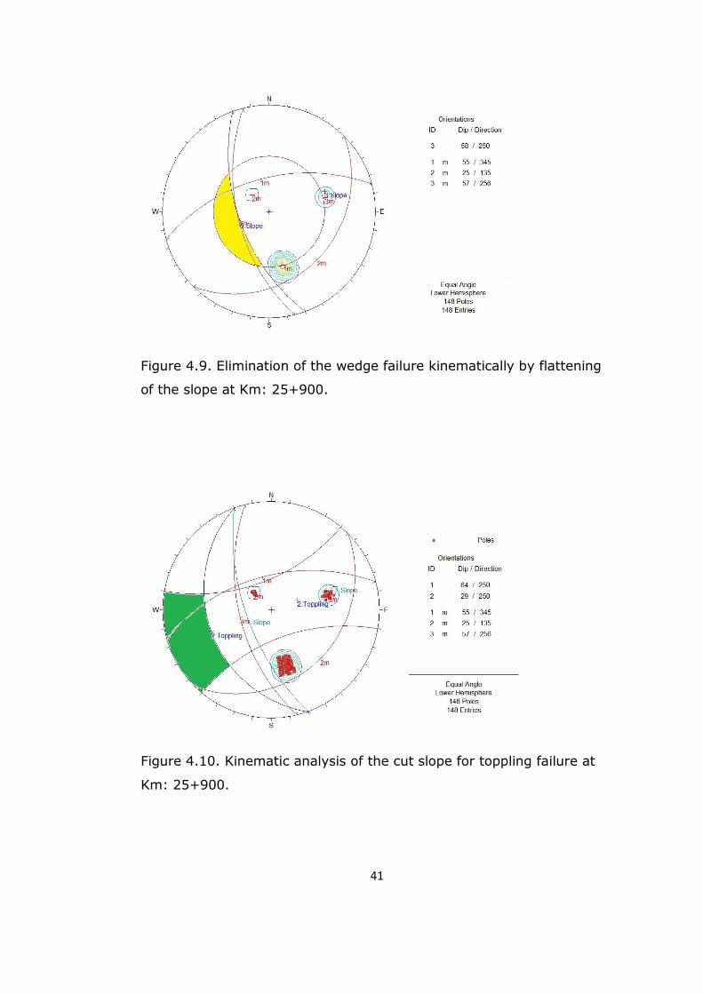
problem, a slope flattening of 8° is suggested (Figure 4.9). The
kinematic analysis for toppling failure reveals that no toppling failure is
likely at this cut slope (Figure 4.10).
Figure 4.8. Kinematic analysis of the cut slope for wedge failure at Km:
25+900.
41
Figure 4.9. Elimination of the wedge failure kinematically by flattening
of the slope at Km: 25+900.
Figure 4.10. Kinematic analysis of the cut slope for toppling failure at
Km: 25+900.
42
As a summary, according to the kinematic analysis carried out at
Km:25+900, the cut slope does not have any toppling failures, but the
planar and wedge failures are likely to occur. 10° of slope flattening will
eliminate both risks. Therefore, only kinematic analysis is performed
for this part of the study area.
4.3. Kinematic Analysis of the Cut Slope at Km: 26+000
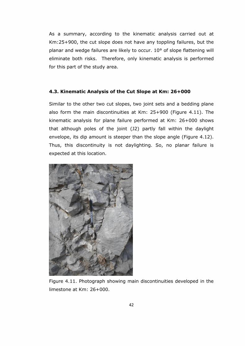
Similar to the other two cut slopes, two joint sets and a bedding plane
also form the main discontinuities at Km: 25+900 (Figure 4.11). The
kinematic analysis for plane failure performed at Km: 26+000 shows
that although poles of the joint (J2) partly fall within the daylight
envelope, its dip amount is steeper than the slope angle (Figure 4.12).
Thus, this discontinuity is not daylighting. So, no planar failure is
expected at this location.
Figure 4.11. Photograph showing main discontinuities developed in the
limestone at Km: 26+000.
43
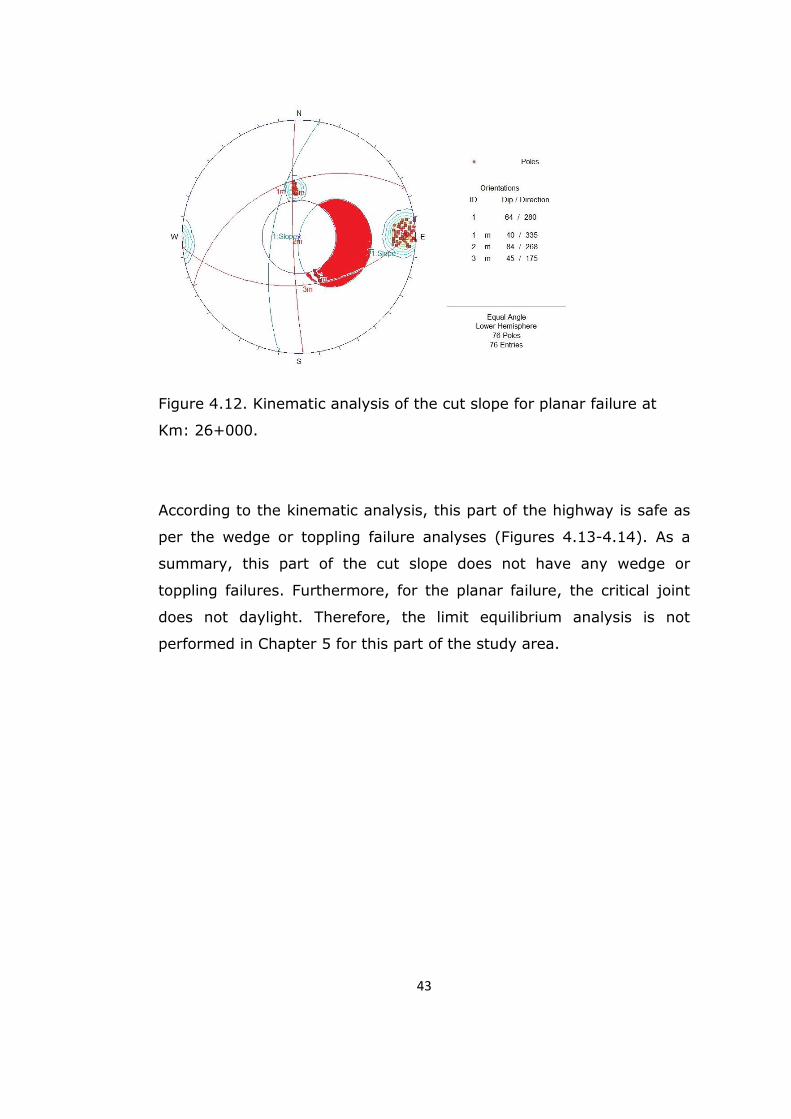
Figure 4.12. Kinematic analysis of the cut slope for planar failure at
Km: 26+000.
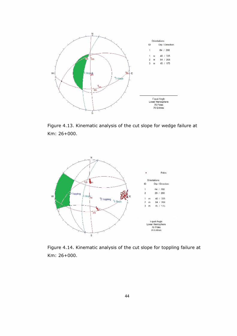
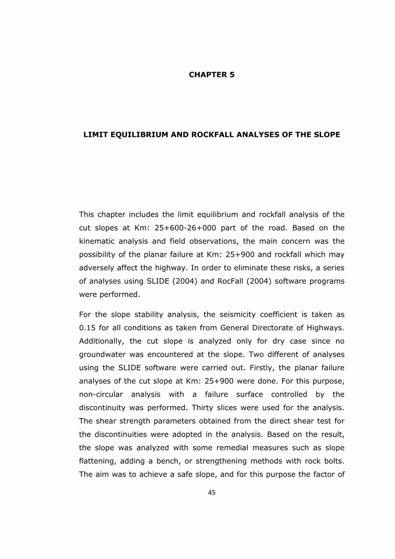
According to the kinematic analysis, this part of the highway is safe as
per the wedge or toppling failure analyses (Figures 4.13-4.14). As a
summary, this part of the cut slope does not have any wedge or
toppling failures. Furthermore, for the planar failure, the critical joint
does not daylight. Therefore, the limit equilibrium analysis is not
performed in Chapter 5 for this part of the study area.
44
Figure 4.13. Kinematic analysis of the cut slope for wedge failure at
Km: 26+000.
Figure 4.14. Kinematic analysis of the cut slope for toppling failure at
Km: 26+000.
45
CHAPTER 5
LIMIT EQUILIBRIUM AND ROCKFALL ANALYSES OF THE SLOPE
This chapter includes the limit equilibrium and rockfall analysis of the
cut slopes at Km: 25+600-26+000 part of the road. Based on the
kinematic analysis and field observations, the main concern was the
possibility of the planar failure at Km: 25+900 and rockfall which may
adversely affect the highway. In order to eliminate these risks, a series
of analyses using SLIDE (2004) and RocFall (2004) software programs
were performed.
For the slope stability analysis, the seismicity coefficient is taken as
0.15 for all conditions as taken from General Directorate of Highways.
Additionally, the cut slope is analyzed only for dry case since no
groundwater was encountered at the slope. Two different of analyses
using the SLIDE software were carried out. Firstly, the planar failure
analyses of the cut slope at Km: 25+900 were done. For this purpose,
non-circular analysis with a failure surface controlled by the
discontinuity was performed. Thirty slices were used for the analysis.
The shear strength parameters obtained from the direct shear test for
the discontinuities were adopted in the analysis. Based on the result,
the slope was analyzed with some remedial measures such as slope
flattening, adding a bench, or strengthening methods with rock bolts.
The aim was to achieve a safe slope, and for this purpose the factor of
46
safety of the final cut slope was aimed as minimum 1.1 for long term
analyses suggested by GDH (1995), Cornforth (2005) and Topal and
Akın (2009). Since there are small pieces and highly jointed structure
in the limestone, secondly, mass failure analysis was carried out. The
aim of this analysis was to find out if there is massive slide of the rock
mass.
For the rockfall analysis, RocFall (2004) software program by
Rocscience was used. This analysis is important because the slopes in
the study area are high and the rocks were blocky. In this type of high
rock slopes, it is generally expected to have rockfalls if the rock is
highly jointed. For this purpose a series of analysis was run for the
different block masses of the rock representing the real field conditions
with the same angle of the slope for the current situation. After
completing the limit equilibrium analyses with remedial measures, the
rockfall analyses are done again in order to see the effects and
differences of flattening the slope or bench.
5.1. Limit Equilibrium Analysis of the Cut Slope for Planar
Failure at Km: 25+900
According to the analysis carried out, this part is found to be the most
problematic part of the highway. It is not safe in the current situation
due to a very low factor of safety of 0.50 with seismic coefficient
(Figures 5.1-5.3).
47
Figure 5.1. Limit equilibrium analysis of the cut slope with discontinuity
controlled failure surface using current highway slope geometry.
Figure 5.2. Limit equilibrium analysis of the cut slope with all surfaces
analysed.
48
Figure 5.3. Limit equilibrium analysis of cut slope with surfaces showing
factor of safety only less than 1.1.
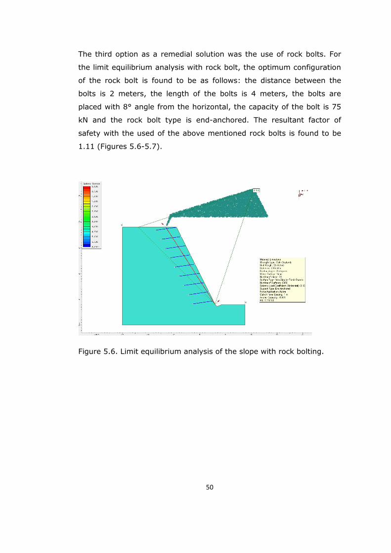
As a remedial solution slope flattening has been utilized. The slope
angle of this part is 64°. Based on the analysis (Figure 5.4), the desired
factor of safety is achieved in case the cut slope is flattened by 7°, thus
forming a new slope with 57°.
Another option was to try benches. The height of the bench was 10
meters from the road elevation. The horizontal length of the bench is
suggested as 5 meters. The limit equilibrium analysis with bench of the
slope yields a stable slope (Figure 5.5).
49
Figure 5.4. Limit equilibrium analysis of the flattened cut slope by 7o.
Figure 5.5. Limit equilibrium analysis of the slope with bench.
50
The third option as a remedial solution was the use of rock bolts. For
the limit equilibrium analysis with rock bolt, the optimum configuration
of the rock bolt is found to be as follows: the distance between the
bolts is 2 meters, the length of the bolts is 4 meters, the bolts are
placed with 8° angle from the horizontal, the capacity of the bolt is 75
kN and the rock bolt type is end-anchored. The resultant factor of
safety with the used of the above mentioned rock bolts is found to be
1.11 (Figures 5.6-5.7).
Figure 5.6. Limit equilibrium analysis of the slope with rock bolting.
51
Figure 5.7. Limit equilibrium analysis of the slope with the rock bolting
and all surfaces analysed.
5.2. Limit Equilibrium Analysis of the Cut Slope for Mass Failure
at Km: 25+900
The aim of this analysis is to find out if there is massive failure in the
cut slope at Km: 25+900. In order to carry out the analyses, RocLab
(2007) software program of Rocscience was used to get the
instantaneous cohesion (c) and the friction angle (ø) values for the
specific slope height. The input and the output values used for the
analysis were as follows:
Inputs:
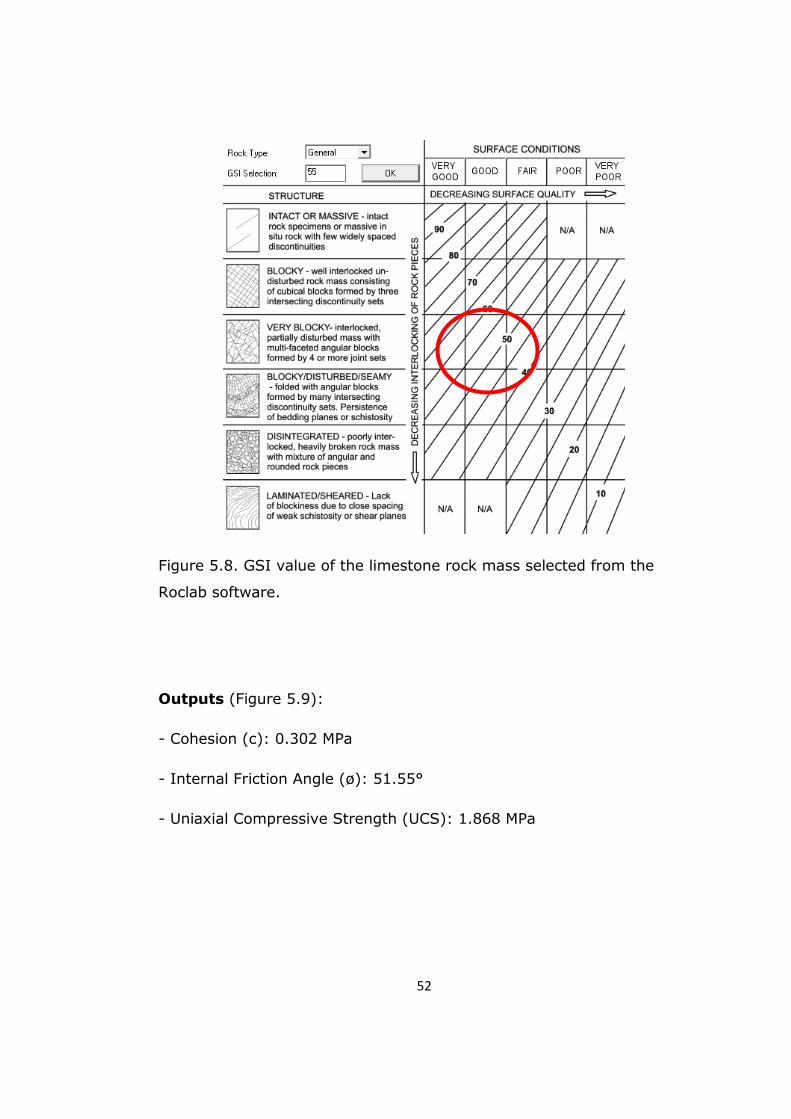
- Intact Uniaxial Compressive Strength (sigci): 50
- GSI (Geological Strength Index): 55 (Figure 5.8)
- Intact Rock Parameter (mi): 8 (Micritic limestone)
- Disturbance Factor (D): 0.7 (Good blasting slope)
52
Figure 5.8. GSI value of the limestone rock mass selected from the
Roclab software.
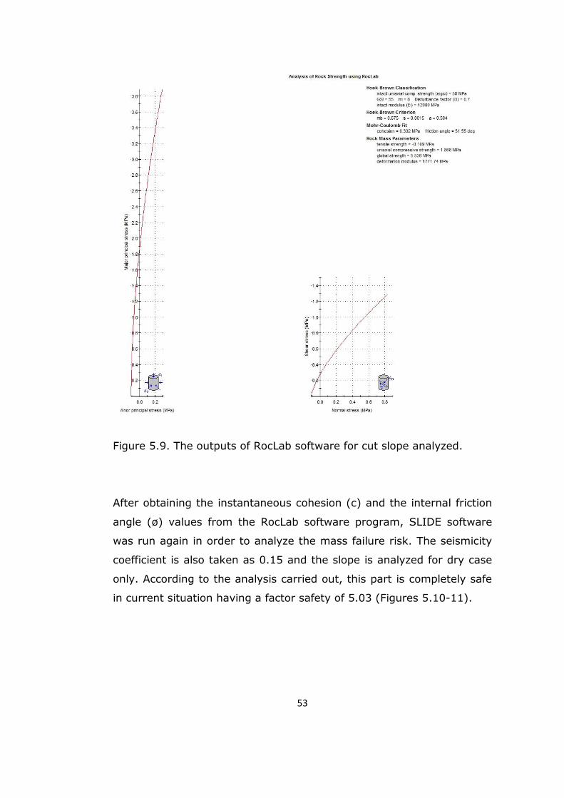
Outputs (Figure 5.9):
- Cohesion (c): 0.302 MPa
- Internal Friction Angle (ø): 51.55°
- Uniaxial Compressive Strength (UCS): 1.868 MPa
53
Figure 5.9. The outputs of RocLab software for cut slope analyzed.
After obtaining the instantaneous cohesion (c) and the internal friction
angle (ø) values from the RocLab software program, SLIDE software
was run again in order to analyze the mass failure risk. The seismicity
coefficient is also taken as 0.15 and the slope is analyzed for dry case
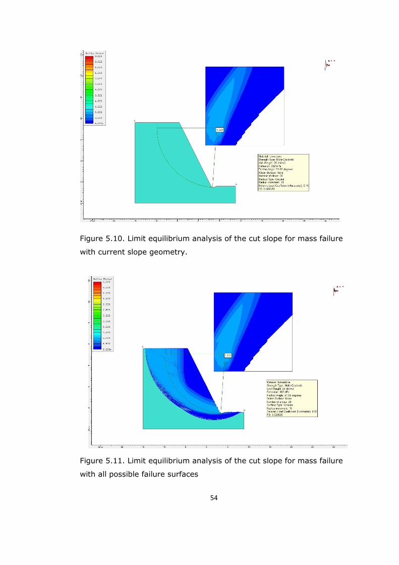
only. According to the analysis carried out, this part is completely safe
in current situation having a factor safety of 5.03 (Figures 5.10-11).
54
Figure 5.10. Limit equilibrium analysis of the cut slope for mass failure
with current slope geometry.
Figure 5.11. Limit equilibrium analysis of the cut slope for mass failure
with all possible failure surfaces
55
As a remedial solution for Km: 25+900, slope flattening has been
suggested. In order to see the effects of this remedial solution for the
mass failure, limit equilibrium analysis is done. The slope angle of this
part was 64° but for the slope flattening solution of Km:25+900, it was
changed as 57°. The resultant factor of safety is found to be 5.27
(Figures 5.12 and 5.13).
Figure 5.12. Limit equilibrium analysis of the cut slope for mass failure
after slope flattening.
56
Figure 5.13. Limit equilibrium analysis of the cut slope for mass failure
after slope flattening with all possible failure surfaces.
As another remedial solution for Km: 25+900, bench has been
suggested. In order to see the effects of this remedial solution for the
mass failure, limit equilibrium analysis is also done. Another reason to
run the limit equilibrium analysis for mass failure in bench solution is
that according to the General Directorate of Highway, the slopes cannot
be higher than 10 meters without benches. The height of the bench is
planned as 10 meters from the road elevation. The horizontal length of
the bench is suggested as 5 meter, as indicated before. The resultant
factor of safety is found to be 5.56 (Figures 5.14 and 5.15).
57
Figure 5.14. Limit equilibrium analysis of the cut slope with bench for
mass failure.
Figure 5.15. Limit equilibrium analysis of the cut slope with bench and
all possible failure surfaces for mass failure.
58
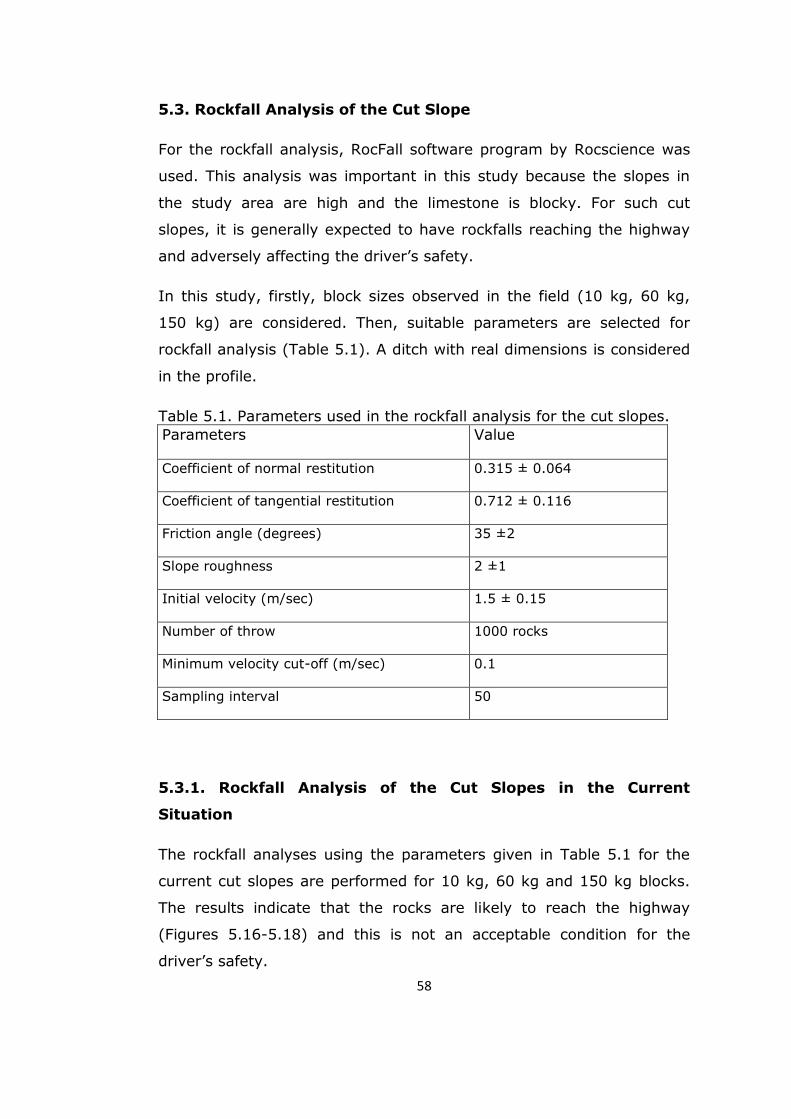
5.3. Rockfall Analysis of the Cut Slope
For the rockfall analysis, RocFall software program by Rocscience was
used. This analysis was important in this study because the slopes in
the study area are high and the limestone is blocky. For such cut
slopes, it is generally expected to have rockfalls reaching the highway
and adversely affecting the driver’s safety.
In this study, firstly, block sizes observed in the field (10 kg, 60 kg,
150 kg) are considered. Then, suitable parameters are selected for
rockfall analysis (Table 5.1). A ditch with real dimensions is considered
in the profile.
Table 5.1. Parameters used in the rockfall analysis for the cut slopes.
Parameters Value
Coefficient of normal restitution 0.315 ± 0.064
Coefficient of tangential restitution 0.712 ± 0.116
Friction angle (degrees) 35 ±2
Slope roughness 2 ±1
Initial velocity (m/sec) 1.5 ± 0.15
Number of throw 1000 rocks
Minimum velocity cut-off (m/sec) 0.1
Sampling interval 50
5.3.1. Rockfall Analysis of the Cut Slopes in the Current
Situation
The rockfall analyses using the parameters given in Table 5.1 for the
current cut slopes are performed for 10 kg, 60 kg and 150 kg blocks.
The results indicate that the rocks are likely to reach the highway
(Figures 5.16-5.18) and this is not an acceptable condition for the
driver’s safety.
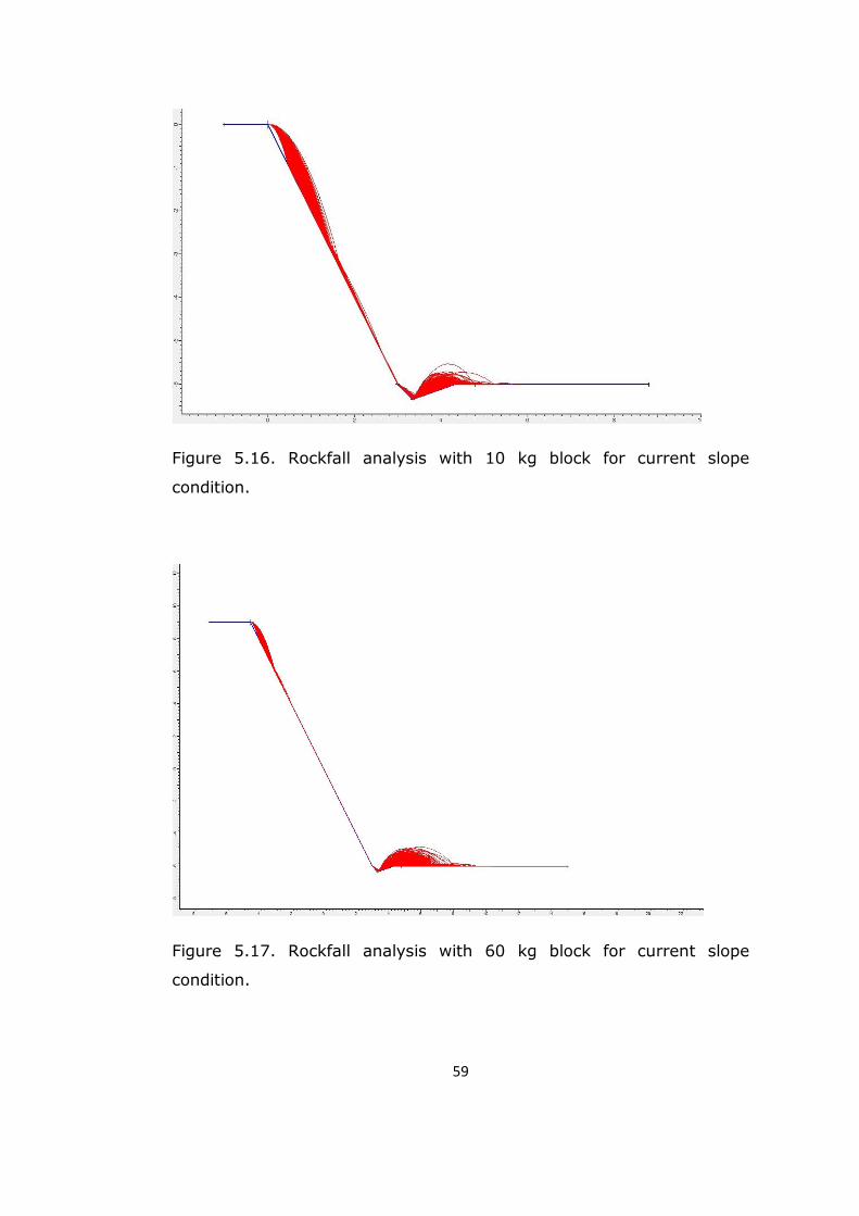
59
Figure 5.16. Rockfall analysis with 10 kg block for current slope
condition.
Figure 5.17. Rockfall analysis with 60 kg block for current slope
condition.
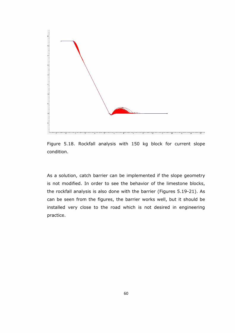
60
Figure 5.18. Rockfall analysis with 150 kg block for current slope
condition.
As a solution, catch barrier can be implemented if the slope geometry
is not modified. In order to see the behavior of the limestone blocks,
the rockfall analysis is also done with the barrier (Figures 5.19-21). As
can be seen from the figures, the barrier works well, but it should be
installed very close to the road which is not desired in engineering
practice.
61
Figure 5.19. Rockfall analysis with 10 kg block and barrier solution for
current slope condition.
Figure 5.20. Rockfall analysis with 60 kg block and barrier solution for
current slope condition.
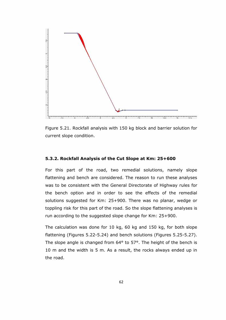
62
Figure 5.21. Rockfall analysis with 150 kg block and barrier solution for
current slope condition.
5.3.2. Rockfall Analysis of the Cut Slope at Km: 25+600
For this part of the road, two remedial solutions, namely slope
flattening and bench are considered. The reason to run these analyses
was to be consistent with the General Directorate of Highway rules for
the bench option and in order to see the effects of the remedial
solutions suggested for Km: 25+900. There was no planar, wedge or
toppling risk for this part of the road. So the slope flattening analyses is
run according to the suggested slope change for Km: 25+900.
The calculation was done for 10 kg, 60 kg and 150 kg, for both slope
flattening (Figures 5.22-5.24) and bench solutions (Figures 5.25-5.27).
The slope angle is changed from 64° to 57°. The height of the bench is
10 m and the width is 5 m. As a result, the rocks always ended up in
the road.
63
Figure 5.22. Rockfall analysis with 10 kg block and slope flattening
solution at Km: 25+600.
Figure 5.23. Rockfall analysis with 60 kg block and slope flattening
solution at Km: 25+600.
64
Figure 5.24. Rockfall analysis with 150 kg block and slope flattening
solution at Km: 25+600.
Figure 5.25. Rockfall analysis with 10 kg block and bench solution at
Km: 25+600.
65
Figure 5.26. Rockfall analysis with 60 kg block and bench solution at
Km: 25+600.
Figure 5.27. Rockfall analysis with 150 kg block and bench solution at
Km: 25+600.
66
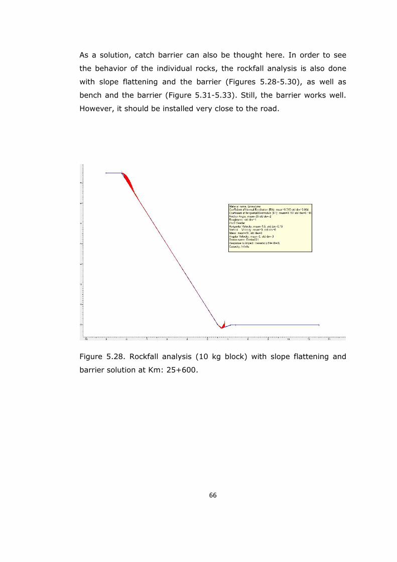
As a solution, catch barrier can also be thought here. In order to see
the behavior of the individual rocks, the rockfall analysis is also done
with slope flattening and the barrier (Figures 5.28-5.30), as well as
bench and the barrier (Figure 5.31-5.33). Still, the barrier works well.
However, it should be installed very close to the road.
Figure 5.28. Rockfall analysis (10 kg block) with slope flattening and
barrier solution at Km: 25+600.
67
Figure 5.29. Rockfall analysis (60 kg block) with slope flattening and
barrier solution at Km: 25+600.
Figure 5.30. Rockfall analysis (150 kg block) with slope flattening and
barrier solution at Km: 25+600.
68
Figure 5.31. Rockfall analysis (10 kg block) with bench and barrier
solution at Km: 25+600.
Figure 5.32. Rockfall analysis (60 kg block) with bench and barrier
solution at Km: 25+600.
69
Figure 5.33. Rockfall analysis (150 kg block) with bench and barrier
solution at Km: 25+600.
Based on the rockfall analyses, one can say that the rocks falling from
the upper part of the slope do not fall to the road. The bench holds all
the rocks. Therefore, benching may be suggested at Km: 25+600 for
the upper part of the slope from rockfall point of view.
5.3.3. Rockfall Analysis of the Cut Slope at Km: 25+900
This part of the highway was found to be problematic according to the
limit equilibrium analysis. In order to be consistent with those
calculations and see the results of the solutions suggested for those
slopes, the rockfall analyses were performed again. The calculation was
done for 10 kg, 60 kg and 150 kg, for both slope flattening (Figures
5.34-5.36) and bench solutions (Figures 5.37-5.39). The slope angle
was changed from 64° to 57°. The height of the bench is 10 m and the
width is 5 m. The analyses reveal that the rocks always ended up in the
road.
70
Figure 5.34. Rockfall analysis (10 kg block) with slope flattening
solution at Km: 25+900.
Figure 5.35. Rockfall analysis (60 kg block) with slope flattening
solution at Km: 25+900.
71
Figure 5.36. Rockfall analysis (150 kg block) with slope flattening
solution at Km: 25+900.
Figure 5.37. Rockfall analysis (10 kg block) with bench solution at Km:
25+900.
72
Figure 5.38. Rockfall analysis (60 kg block) with bench solution at Km:
25+900.
Figure 5.39. Rockfall analysis (150 kg block) with bench solution at
Km: 25+900.
73
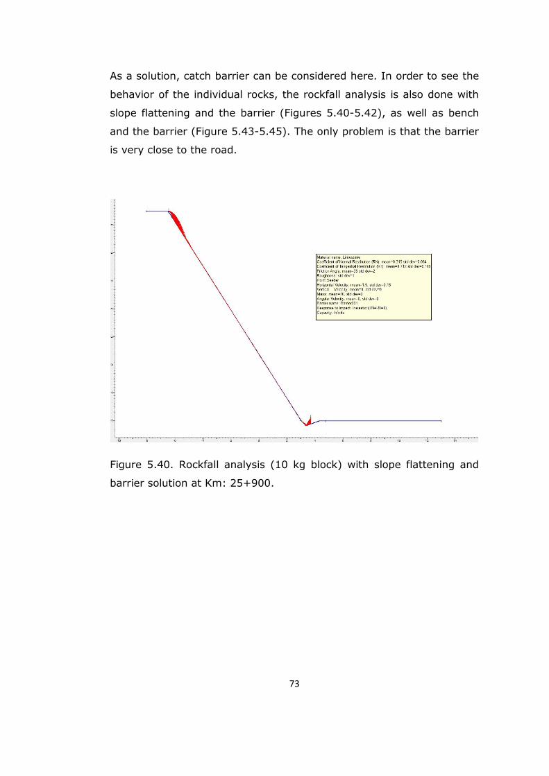
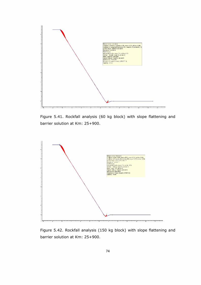
As a solution, catch barrier can be considered here. In order to see the
behavior of the individual rocks, the rockfall analysis is also done with
slope flattening and the barrier (Figures 5.40-5.42), as well as bench
and the barrier (Figure 5.43-5.45). The only problem is that the barrier
is very close to the road.
Figure 5.40. Rockfall analysis (10 kg block) with slope flattening and
barrier solution at Km: 25+900.
74
Figure 5.41. Rockfall analysis (60 kg block) with slope flattening and
barrier solution at Km: 25+900.
Figure 5.42. Rockfall analysis (150 kg block) with slope flattening and
barrier solution at Km: 25+900.
75
Figure 5.43. Rockfall analysis (10 kg block) with bench and barrier
solution at Km: 25+900.
Figure 5.44. Rockfall analysis (60 kg block) with bench and barrier
solution at Km: 25+900.

76
Figure 5.45. Rockfall analysis (150 kg block) with bench and barrier
solution at Km: 25+900.
The rocks falling from the upper part of the slope do not fall again to
the road. The bench holds all the rocks. As for the rockfall point of
view, benching is suggested at Km: 25+900 for the upper part of the
slope.
5.3.4. Rockfall Analysis of the Cut Slope at Km: 26+000
For this part, two remedial solutions, namely slope flattening and bench
are considered during the rockfall analysis. The analysis was done for
both slope flattening (Figures 5.46-5.48) and bench (Figures 5.49-
5.51) solutions with the same block weights. The slope angle was
changed from 64° to 57°. The height of the bench is 10 m and the
width is 5 m. The rockfall analyses show that the falling rocks mainly
reach the road.
77
Figure 5.46. Rockfall analysis (10 kg block) with slope flattening
solution at Km: 26+000.
Figure 5.47. Rockfall analysis (60 kg block) with slope flattening
solution at Km: 26+000.
78
Figure 5.48. Rockfall analysis (150 kg block) with slope flattening
solution at Km: 26+000.
Figure 5.49. Rockfall analysis (10 kg block) with bench solution at Km:
26+000.
79
Figure 5.50. Rockfall analysis (60 kg block) with bench solution at Km:
26+000.
Figure 5.51. Rockfall analysis (150 kg block) with bench solution at
Km: 26+000.
80
As a solution, catch barrier can be considered here. The rockfall
analyses done with slope flattening and the barrier (Figures 5.52-5.54),
and bench and the barrier (Figure 5.55-5.57) show that although the
barriers solve the problem, they are very close to the road. Therefore,
it is preferable to consider other alternatives if the ditch details do not
change.
Figure 5.52. Rockfall analysis (10 kg block) with slope flattening and
barrier solution at Km: 26+000.
81
Figure 5.53. Rockfall analysis (60 kg block) with slope flattening and
barrier solution at Km: 26+000.
Figure 5.54. Rockfall analysis (150 kg block) with slope flattening and
barrier solution at Km: 26+000.
82
Figure 5.55. Rockfall analysis (10 kg block) with bench and barrier
solution at Km: 26+000.
Figure 5.56. Rockfall analysis (60 kg block) with bench and barrier
solution at Km: 26+000.
83
Figure 5.57. Rockfall analysis (150 kg block) with bench and barrier
solution at Km: 26+000.
The rocks falling from the upper part of the slope do not fall again to
the road. The bench holds all the falling rocks. Therefore, from rockfall
point of view, benching is suggested at Km: 26+000 for the upper part
of the slope similar to the other cases.
84
CHAPTER 6
DISCUSSION
This chapter is about the suggested solutions and their comparisons for
the slope stability of the limestone cut slopes (nearly 15 m high)
exposed at Km: 25+600-26+000. As mentioned before, the main
concerns about this particular section of the road are planar failure and
the rockfall issues. In order to eliminate these risks, a series of
kinematic, limit equilibrium and rockfall analyses are done.
The outcrop in Km: 25+600-26+000 belongs to Limestone unit (JKyk)
of the Çataltepe nappe. It is highly fractured and jointed. The rock
mainly contains two joint sets and bedding plane as discontinuities. The
main issue for this part of the road is the planar failure and rockfall that
could assessed through limit equilibrium and rockfall analyses, and
visual observations in the field.
For the current situation, it has been seen that there is no risk for mass
failure. However, the planar failure is expected at Km: 25+900. This
could be eliminated by 7o slope flattening. Thus, the new slope may be
57o instead of 64o. Similarly, rock bolting may be applied to stabilize
the slope. Due to the height of the cut slopes, there is a necessity to
include a bench for the slopes studied. In this case, no planar failure is
expected as validated by the limit equilibrium analysis. A comparison of
85
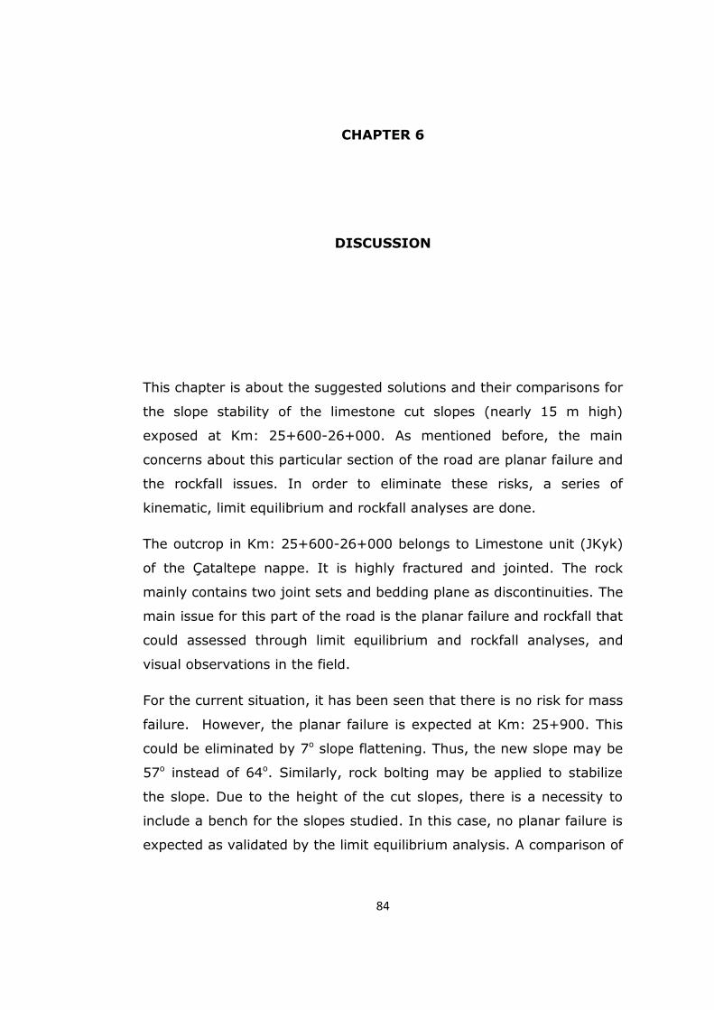
factor of safeties for different solutions and different parts of the
section can be seen in Table 6.1.
Table 6.1. Comparison of the factor of safety values from the limit equilibrium analysis at Km: 25+900.
Factor of Safety
along Discontinuity Factor of Safety for Mass Failure
Exsiting Slope 0.50 5.03
Slope with Bench Stable 5.56
Slope Flattening Stable 5.27
Slope with Rock Bolt 1.11 -
Although all of these approaches seem to solve the slope instability
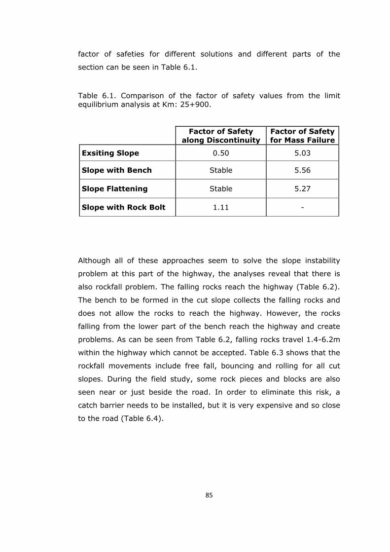
problem at this part of the highway, the analyses reveal that there is
also rockfall problem. The falling rocks reach the highway (Table 6.2).
The bench to be formed in the cut slope collects the falling rocks and
does not allow the rocks to reach the highway. However, the rocks
falling from the lower part of the bench reach the highway and create
problems. As can be seen from Table 6.2, falling rocks travel 1.4-6.2m
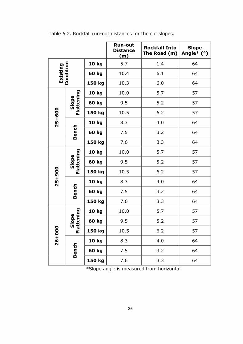
within the highway which cannot be accepted. Table 6.3 shows that the
rockfall movements include free fall, bouncing and rolling for all cut
slopes. During the field study, some rock pieces and blocks are also
seen near or just beside the road. In order to eliminate this risk, a
catch barrier needs to be installed, but it is very expensive and so close
to the road (Table 6.4).
86
Table 6.2. Rockfall run-out distances for the cut slopes.
Run-out Distance
(m)
Rockfall Into The Road (m)
Slope Angle* (°)
Exis
tin
g
Co
nd
itio
n
10 kg 5.7 1.4 64
60 kg 10.4 6.1 64
150 kg 10.3 6.0 64
25
+6
00
Slo
pe
Fla
tten
ing
10 kg 10.0 5.7 57
60 kg 9.5 5.2 57
150 kg 10.5 6.2 57
Ben
ch
10 kg 8.3 4.0 64
60 kg 7.5 3.2 64
150 kg 7.6 3.3 64
25
+9
00
Slo
pe
Fla
tten
ing
10 kg 10.0 5.7 57
60 kg 9.5 5.2 57
150 kg 10.5 6.2 57
Ben
ch
10 kg 8.3 4.0 64
60 kg 7.5 3.2 64
150 kg 7.6 3.3 64
26
+0
00
Slo
pe
Fla
tten
ing
10 kg 10.0 5.7 57
60 kg 9.5 5.2 57
150 kg 10.5 6.2 57
Ben
ch
10 kg 8.3 4.0 64
60 kg 7.5 3.2 64
150 kg 7.6 3.3 64
*Slope angle is measured from horizontal
87
Table 6.3. Types of rockfall movements at the cut slopes.
Free Fall Rolling Bouncing
Exis
tin
g
Co
nd
itio
n
10 kg x x x
60 kg x x x
150 kg x x x
25
+6
00
Slo
pe
Fla
tten
ing
10 kg x x x
60 kg x x x
150 kg x x x
Ben
ch
10 kg x x x
60 kg x x x
150 kg x x x
25
+9
00
Slo
pe
Fla
tten
ing
10 kg x x x
60 kg x x x
150 kg x x x
Ben
ch
10 kg x x x
60 kg x x x
150 kg x x x
26
+0
00
Slo
pe
Fla
tten
ing
10 kg x x x
60 kg x x x
150 kg x x x
Ben
ch
10 kg x x x
60 kg x x x
150 kg x x x
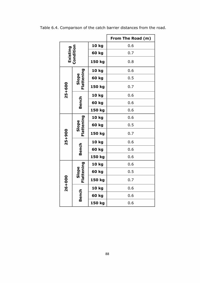
88
Table 6.4. Comparison of the catch barrier distances from the road.
From The Road (m)
Exis
tin
g
Co
nd
itio
n
10 kg 0.6
60 kg 0.7
150 kg 0.8 2
5+
60
0
Slo
pe
Fla
tten
ing
10 kg 0.6
60 kg 0.5
150 kg 0.7
Ben
ch
10 kg 0.6
60 kg 0.6
150 kg 0.6
25
+9
00
Slo
pe
Fla
tten
ing
10 kg 0.6
60 kg 0.5
150 kg 0.7
Ben
ch
10 kg 0.6
60 kg 0.6
150 kg 0.6
26
+0
00
Slo
pe
Fla
tten
ing
10 kg 0.6
60 kg 0.5
150 kg 0.7
Ben
ch
10 kg 0.6
60 kg 0.6
150 kg 0.6
89
Regarding the remedial measures, any combination of slope flattening,
benching, rock bolting, wire mesh and shotcrete application may be
considered. Nevertheless, benching is compulsory for such heights of
the cut slopes. No failure is expected in such a case based on the limit
equilibrium analysis, but there is a problem of rockfall which may reach
the road. Therefore, either catch barriers must be installed or individual
rock pieces should be stabilized. The catch barriers are expansive and
should be installed close to the highway if the ditch design is not
changed. On the basis of all the field observations and stability-rockfall
analyses, the author of this thesis suggests that after benching (10 m
high and 5 m wide), the use of wire mesh+shotcrete is expected to
eliminate the rockfall problems. Although various types of shotcrete
exist, fibre-reinforced shotcrete is recommended for the cut slopes
studied in this thesis because it is the most efficient method in slope
stabilization, more adoptable to the topography and it reduces the
amount of shotcrete mix to be used and labor cost (Ballou and
Niermann, 2002).
90
CHAPTER 7
CONCLUSIONS AND RECOMMENDATIONS
This thesis is aimed to investigate the engineering geological properties
of the units exposed for Km: 25+600-26+000 at three cut slopes along
Antalya-Korkuteli road from the slope stability point of view. Based on
the field studies as well as kinematic, limit equilibrium and rockfall
analyses, the following conclusions and recommendations are
achieved:
1. The main rock type exposed in the study area is limestone.
2. The limestone at the cut slopes are beige to gray, fine grained,
fossiliferous, and highly jointed. The rock contains two joint sets
and a bedding plane as main discontinuities. The discontinuities
have close to wide spacing, tight to partly open aperture, planar
rough to undulating rough discontinuity surfaces. It is slightly
weathered mainly in the form of discoloration along discontinuity
surfaces with some karstic cavities exists near the surface. The
rock is medium strong and strong. The discontinuities are
generally free of infilling. However, local calcite infilling may be
seen. One of the joint set is bed confined. However, the other
discontinuities are persistent. The cut slopes are dry.
3. Based on the kinematic analysis, planar failure is expected at Km:
25+900. Limit equilibrium analysis reveal that 7o slope flattening
91
may solve the instability problem. Since bench with 10 m high
and 5 m wide is required, then the slope becomes stable with the
new slope geometry. Additionally, rockfall problems are expected
at all three cut slopes. Benching eliminates rockfall from upper
part of the cut slope, but the rockfalls from the lower part still
reach the road.
4. As a remedial measure, following the bench construction with a
slope angle of 64o, covering the cut slope with wire mesh and
fibre reinforced shotcrete will eliminate the rockfall problem.
92
REFERENCES
Antalya Agriculture, 2007, http://www.antalya-tarim.gov.tr/
haber_detay.asp?ID=59&baslik_id=66, last accessed date: 10/09/2008
Antalya Municipality 2007a, Climate http://www.antalya.bel.tr/tr/
kent_profili/iklim.cfm?tanitimId=761, last accessed date: 10/09/2008
Antalya Municipality 2007b, Vegetation http://www.antalya.bel.tr/tr/
kent_profili/cografya.cfm?tanitimId=852, last accessed date:
10/09/2008
Ballou, M. and Matt Niermann, M., 2002, Soil and rock slope
stabilization using fiber-reinforced shotcrete in North America,
Shotcrete, 20-23.
Colin, H. J., 1962, Fethiye-Antalya-Kaş-Finike (Güneybatı Anadolu)
Bölgesinde Yapılan Jeolojik Etüdler. Bulletin of the Mineral Research
and Exploration Institute of Turkey, no. 59, 19-60
Cornforth, D.H., 2005, Landslides in practice. Wiley, Hoboken, 596 p.
DIPS, 2004, Scientific Software- Data Interpretation Package using
Stereographic projection, Version 5.103, Rocscience Inc., Canada, 90 p
93
Form Jeoteknik, 2008, Antalya-Korkuteli Yolu Mühendislik Jeolojisi
Raporu, Ankara
GDDA, 1996. Earthquake zoning map of Turkey, General Directorate of
Disaster Affairs, Ministry of Reconstruction and Resettlement of Turkey.
GDH, 1995, Zemin arastırma işine ait teknik şartname. Karayolları
Genel Müdürlüğü, Ankara
GDH, 2007, General Directorate of Highways website,
http://www.kgm.gov.tr/, last accessed date: 10/09/2008
Google Earth, 2010, Maps and satellite images for complex or
pinpointed regional searches
Hoek, E., Bray, J.W., 1981, Rock Slope Engineering, 3rd ed. Institute of
Mining and Metallurgy, London. 358 p.
ISRM (International Society for Rock Mechanics), 1981, Rock
characterization, testing and monitoring – ISRM Suggested Methods,
Pergamon Press, Oxford, Brown, E.T.(ed), 211 p.
MTA, 2004, Türkiye 1:500.000 Ölçekli Jeoloji Haritası
Poisson, A. 1977, Recherches g.ologiques dans les Taurides
occidentals. These Doct. D’Etat, Universitie de Paris-Sud, Orsay, 795 p.
Poisson, A. and Poignant, A.F., 1974, La formation ele Karabayır, base
de la transgression Miocene dans la region de Korkuteli (Turquie).
Bulletin of the Mineral Research and Exploration Institute of Turkey, no.
82, 67-71
94
Priest, S.D., 1993, Discontinuity analysis for rock engineering.
Chapman & Hall, London, 496p.
RocFall, 2004, Scientific Software-Statistical Analysis of Rockfalls,
Version 4.039, Rocscience Inc., Canada, 65 p
RocLab, 2007, Scientific Software-Rock Mass Strength Parameters,
Version 1.031, Rocscience Inc., Canada, 25 p
SLIDE, 2004, Scientific Software-2D Limit Equilibrium Slope Stability
Analysis, Version 5.104, Rocscience Inc., Canada, 199 p
Şenel, M., 1997, 1:100.000 Ölçekli Isparta K-10 Paftası. MTA Genel
Müdürlüğü, pp. 3-10.
Şenel, M., Akdeniz, N., Öztürk, E. M., Özdemir, T., Kadınkız, G., Metin,
Y., Öcal, H., Serdaroğlu, M., Örçen, S., 1994, Fethiye (Muğla)-Kalkan
(Antalya) ve Kuzeyinin Jeolojisi. Maden Tetkik ve Arama Genel
Müdürlüğü Jeoloji Etütleri Dairesi Başkanlığı, pp. 13-15.
Topal, T., Akin, M., 2009, Geotechnical assessment of a landslide along
a natural gas pipeline for possible remediations (Karacabey-Turkey),
Environmental Geology, 57 (3): 611-620.
Turner, A.K., Schuster, R.L., 1996, Landslides-investigation and
mitigation. Transportation Research Board, National Research Council,
Special Report, vol. 247. National Academy Press, Washington, DC. 673
p.