Assessment of the Performance of Image Fusion for the Mapping of SnowUsing Euclidean Distance

Pascal Sirguey1, Sven Oltmer2 & Renaud Mathieu1

1Global Land Ice Measurements from Space (GLIMS) New Zealand OfficeSchool of Surveying, University of Otago, PO Box 56, Dunedin, New Zealand

Phone: +64 3 479-7591 Fax: +64 3 479-7586Email: sirpa271@student.otago.ac.nz

Email: renaud.mathieu@stonebow.otago.ac.nz

2 Institute for Applied Photogrammetry and Geoinformatics (IAPG)Department of Civil Engineering and Geoinformation

University of Applied Sciences Oldenburg/Ostfriesland/WilhelmshavenOfener Strae 16-19, D-26121 Oldenburg, Germany

Email: sven.oltmer@stud.fh-oldenburg.de

Presented at SIRC 2007 - The 19th Annual Colloquium of the Spatial Information Research CentreUniversity of Otago, Dunedin, New Zealand

December 6th-7th 2007

ABSTRACT

The assessment of the performance of multi-resolution image fusion, or image sharpening meth-ods, is difficult. In the context of binary classification of snow targets in mountainous terrain, fusionmethods were applied to help achieve more accurate mapping. To quantify objectively the gain of in-formation that can be attributed to an increase in spatial resolution, we investigate the Mean EuclideanDistance (MED) between the snowline obtained from the classification, and a reference snowline (ora ground truth line), as a relevant indicator to measure both the discrepancy between datasets at differ-ent spatial resolutions, and the accuracy of the mapping process. First, a theoretical approach basedon aggregating detailed reference images from the Advanced Spaceborne Thermal Emission and Re-flection Radiometer (ASTER) showed that the MED has a linear relationship with the pixel size thatmakes it suitable to assess images of different resolutions. Secondly, we tested the MED to snowmaps obtained ‘with’ or ‘without’ applying a fusion method to the MODerate Resolution ImagingSpectroradiometer (MODIS). We demonstrated that the MED identified a significant value added, interms of mapping accuracy, which can be attributed to the fusion process. When the fusion methodwas applied to four different images, the MED overall decreased by more than 30%. Finally, such a‘feature based’ quality indicator can also be interpreted as a statistical assessment of the planimetricaccuracy of natural pattern outlines.

Keywords and phrases: Image fusion, Image sharpening, Metric, Snow, Snowline, Remote sensing, Euclideandistance, MODIS

1 INTRODUCTIONIn the context of remote sensing, image fusion consists of merging images from different sources, which hold

information of a different nature, to create a synthesized image that retains the most desirable characteristics ofeach source (Pohl & Genderen 1998, Zhang 2004, Amolins, Zhang & Dare 2007). For instance, many opticalsensors (e.g. SPOT, IKONOS, QUICKBIRD) routinely acquire simultaneously one panchromatic image (PAN),covering a wide part of the electromagnetic spectrum, and one multispectral image (MS), including several bandsat a coarser spatial resolution (i.e. pixel size). Other sensors, such as the MODerate Resolution Imaging Spectro-radiometer (MODIS) or the Advanced Spaceborne Thermal Emission and Reflection Radiometer (ASTER), donot hold a PAN band, but numerous spectral bands with different spatial resolutions. In this context, multispectralfusion methods usually aim to merge the rich spatial content of a high spatial resolution image (HR, e.g. PANband) with the rich spectral content of a low spatial resolution image (LR, e.g. MS bands) (Garguet-Duport, Girel,

Chassery & Pautou 1996, Ranchin, Aiazzi, Alparone, Baronti & Wald 2003, Gonzalez-Audicana, Saleta, Catalan& Garcıa 2004, Tu, Huang, Hung & Chang 2004, Zhang & Kang 2006). Fusion is becoming popular in variousfield due to its ability to improve the detection and extraction of ground targets (Nichol & Wong 2005, Lasaponara& Masini 2005, Malpica 2007), or the spatial resolution of post-classified products (Pasqualini, Pergent-Martini,Pergent, Agreil, Skoufas, Sourbes & Tsirika 2005, Jin & Davis 2005, Sirguey, Mathieu, Arnaud, Khan & Chanus-sot 2008). In most cases the assessment of the quality of the fusion or the gain of information obtained throughthe fusion remains challenging.

In order to improve the details of snow maps in mountainous terrain, Sirguey et al. (2008) proposed to fuse therich spatial content of the 250-m resolution MODIS HR bands into the 500-m resolution MODIS LR bands thatare spectrally required to map the snow. The method was validated by comparing MODIS-derived snow maps,obtained ‘without’ or ‘with’ the fusion process, with reference maps obtained simultaneously from 15-m resolu-tion ASTER imagery. A visual analysis eventually concluded an improvement in the ability to map snow with thefused images. However, this subjective method does not provide a quantitative measure that would objectivelyscore the improvement. Therefore both integrated and pixel-based metrics were investigated. Nevertheless, com-paring images of different resolution is difficult and raises the issue of multi-scale analysis (Woodcock & Strahler1987, Lam & Quattrochi 1992). Not all metrics are adequate to assess the gain of information generated by anincrease of spatial resolution (Sirguey et al. 2008). Pixel-based metrics should be established with maps havingthe same spatial resolution, in order to be comparable. Consequently, the 250-m resolution maps of subpixelsnow fraction were aggregated at 500 m prior to computing the pixel-based metrics. This approach demonstratedthat the fusion significantly add information, but it cannot truly account for the fact that the snow was mapped atan improved resolution of 250-m pixel size. A metric capable of operating independently from the pixel size istherefore desirable.

In this article, we propose to investigate the potential of the Mean Euclidean Distance (MED) between theseasonal snowlines extracted from the MODIS-derived snow maps (either at 500-m or 250-m spatial resolution,i.e. ‘without’ or ‘with’ fusion) and the reference ASTER snowline, as a relevant metric to assess the gain that thefusion provides in terms of snow cover delineation capability. We based our reasoning on the fact that edges andcontours are essential in the understanding of natural scenes, and therefore the better the contours are depicted, thehigher the quality of the image (Zhai, Zhang, Yang & Xu 2005). In the first part of this article, we briefly reviewthe strategies and issues raised by the quality assessment of fused products. In the second part, we present the dataand the methodology implemented to assess the performance of the MED as a metric. Finally, we present anddiscuss the sensitivity of this metric to various parameters, and its efficiency when applied to the MODIS-derivedsnow maps obtained ‘without’ or ‘with’ implementing the fusion method.

2 BACKGROUND ON QUALITY ASSESSMENT OF MULTISPECTRAL FUSIONImage fusion algorithms often create radiometric distortions and/or artefacts (Wald, Ranchin & Mangolini

1997, Du, Vachon & van der Sanden 2003, Tu et al. 2004, Gonzalez-Audicana, Otazu, Fors & Alvarez-Mozos2006). Therefore, it is required to estimate the quality of the fusion process, in order to assess its performanceand robustness, as well as the usability of the fused product. The validation of image fusion is a difficult task,which usually rely on the investigation of both subjective and objective methods (Aiazzi, Alparone, Argenti &Baronti 1999, Gao, Wang & Li 2005, Shi, Zhu, Tian & Nichol 2005, Laporterie-Dejean, de Boissezon, Flouzat &Lefevre-Fonollosa 2005, Alparone, Wald, Chanussot, Thomas, Gamba & Bruce 2007, Petrovic 2007).

2.1 Qualitative analysisSubjective methods are based on the visual analysis of the fused image. They aim to provide a judgment

(e.g. an opinion score) on the quality of the fused product according to a prior set of criteria, defined withregard to the needs of the users (Petrovic 2007, Laporterie-Dejean et al. 2005). However, because it involves thesubjective human visual perception, such qualitative assessment is inevitably biased by the observer’s experiencesand appreciation (Toet & Franken 2003, Chen & Varshney 2007). Visual analysis is a powerful tool to assessimprovement, because of its ability to capture spatial details as the resolution of the image increases, but it failsto account accurately for the preservation of the radiometry in the image. Therefore its consistency in terms ofscientific value with regard to the original data is questionable.

2.2 Quantitavive analysisNumerous researches report on the design of metrics to assess objectively the quality of fused images (Wald

et al. 1997, Ranchin & Wald 2000, Wald 2000, Xydeas & Petrovic 2000, Wang & Bovik 2002, Alparone, Baronti,Garzelli & Nencini 2004). The metrics are usually based on and/or derived from standard descriptive statistics

(e.g. bias or difference of means, Root Mean Square Error RMSE, coefficient of correlation CC, coefficient ofdetermination R2, standard deviation σ). They aim to quantify the discrepancy between the fused image and areference, to measure both the gain of information generated by an increase of spatial resolution, and its spectralintegrity with regard to the original spectral content. Since no reference image is obviously available at the finerresolution (resolution of the fused image) a popular protocol consists in the assessment of the method at a coarserresolution (Wald et al. 1997). HR and LR images are degraded relatively to their resolution so that the pixel size ofthe degraded HR matches the original LR. The fusion process is computed with the degraded images. The originalLR can then be used as a genuine reference in the process of validation. In case of a successful assessment, themethod is assumed to perform similarly at the finer scale.

2.3 Assessment through the validation of end-productsThe validation protocols described previously are limited to the investigation of the fused image itself. They

aim to score the quality of the image that is obtained with the fusion, with regard to the theoretical image thatwould have been acquired if the sensor had the desired spatial resolution. Sometimes, however, the imagesobtained from the fusion are to be post-processed (e.g. semantic classification of ground targets, or retrievalof physical parameter), to create a specific end-product with an increased spatial resolution. In this case, therelevancy and performance of the fusion can eventually be measured in terms of the quality of the post-processedproduct, rather than the quality of the fused images only. Such validation strategy aims to prove that there is asignificant improvement in the end-product, if the fusion is processed prior to post-processing the image. It is thisstrategy that we use in the present article. Indeed, we aim to estimate the accuracy, in terms of position, of theseasonal snowline, which can be extracted from MODIS-derived snow maps obtained ‘with’ or ‘without’ usingthe multispectral fusion.

3 DATAFour pairs of simultaneous MODIS/ASTER acquisitions selected at different seasons and including various

conditions of snow cover were selected in the Aoraki/Mount Cook region, New Zealand (see dates in Tab. 1).

3.1 MODIS-derived subpixel snow fraction

1355000

1355000

1385000

1385000

5150

000

5150

000

5180

000

5180

000

0 10Kilometers

(a)

1355000

1355000

1385000

1385000

5150

000

5150

000

5180

000

5180

000

Snow Frac100% 0

0 10Kilometers

(b)

1355000

1355000

1385000

1385000

5150

000

5150

000

5180

000

5180

000

Snow Frac100% 0

0 10Kilometers

(c)

Figure 1: Example of subpixel snow map created from MODIS imagery (Mt Cook Area, South Island of NewZealand, 31 December 2002 22:35 GMT) : (a) False colour RGB composite with MODIS bands 1, 2 (250 m) and3 (fused to 250 m). (b) Subpixel snow fraction computed from MODIS bands at 500 m. (c) Subpixel snow fractioncomputed from MODIS bands fused at 250 m.

The four MODIS images were processed according to the methods described in more details in Sirgueyet al. (2008). These include the following steps: georectification of MODIS-Terra L1B swath data products(MOD02QKM, MOD02HKM, MOD021KM, MOD03), wavelet-based fusion between MODIS 250-m bands and

MODIS 500-m bands, and implementation of a topographic and atmospheric correction model as described byRichter (1998). Finally, a constrained spectral unmixing technique was applied (Keshava 2003), either to theseven original 500-m bands or the seven 250-m bands obtained ‘with’ the fusion, to produce maps of subpixelsnow fractions. Figure 1 shows an example of a MODIS-derived map of subpixel snow fraction. Figure 1(b) andFigure 1(c) show the snow maps obtained ‘without’ and ‘with’ the fusion, at 500 m and 250 m, respectively. Theyillustrate the improvement that can be achieved when implementing the fusion.

3.2 Reference snow cover from ASTERThe four corresponding ASTER images were orthorectified and matched to the MODIS images. An example

showing a simultaneous ASTER/MODIS pair is given in Figure 2(a). The spatial resolution of ASTER (15 m)images compared to the 250 m and 500 m resolution of MODIS images provides a ratio of 277 and 1111 ASTERpixels, respectively, for each MODIS pixel. We therefore hypothesized that a binary classification of snow fromASTER would provide accurate ground truth of the snow cover distribution. The snow was binary classified usingthe Normalized Difference Snow Index (NDSI) that takes advantage of the contrast between the high reflectanceof snow in the green part of the visible spectrum (ASTER Band 1 at 560 nm) and its low reflectance in the shortwave infrared (ASTER Band 4 at 1640 nm) (Equation 1) (Crane & Anderson 1984).

NDSI =ρ∗560nm − ρ∗1640nm

ρ∗560nm + ρ∗1640nm

(1)

where ρ∗ is the apparent reflectance measured at the top of atmosphere by ASTER. A custom threshold of 0.7was chosen to binary classified the snow according to the NDSI value, based on visual analysis of the image andthe investigation of the histogram of the NDSI image. Such a relatively high threshold insures that pixels are fullycovered with snow. From the binary classification, it is possible to extract the reference seasonal snowline, whichstands for the boundary between the group of pixels classified as ‘snow’ or ‘no snow’.

1355000

1355000

1385000

1385000

5120

000

5120

000

5150

000

5150

000

5180

000

5180

000

0 10

Kilometers

(a)

1355000

1355000

1385000

1385000

5120

000

5120

000

5150

000

5150

000

5180

000

5180

000

0 10

Kilometers

(b)

Figure 2: Example of simultaneous ASTER and MODIS imagery (Mt Cook Area, South Island of New Zealand, 31December 2002 22:35 GMT) : (a) False colour RGB composite from ASTER bands 2, 3, 1 (15 m) overlaid ontoa false colour RGB composite from MODIS bands 1, 2 (250 m) and 3 (fused to 250 m). The difference of spatialresolution is clearly visible when zooming in the pdf version of this document. (b) Binary snow map from ASTERused as reference and overlaid onto the MODIS RGB composite (pixels classified as snow are drawn in black;pixels without snow are transparent).

4 METHODOLOGY4.1 Object-based metrics

The quality assessment of classified end-products or maps is usually based on a ‘per-pixel’ approach. It refersto the assessment of agreement and confusions that occur between the classified image and the ground or a more

detailed reference image. Recently, object-based indicators have also been developed to provide a more compre-hensive assessment of the quality of geo-spatial objects (Zhan, Molenaar, Tempfli & Shi 2005). In an object-basedenvironment, Zhan et al. (2005) suggested that new measures accounting for the correct classification, size andposition of the objects, can be used along with ‘per-pixel’ measures to assess quality. Li, He, Bu, Wen, Chang,Hu & Li (2005) also investigated the behaviour of numerous simple and sophisticated geo-spatial metrics to sev-eral parameters, such as number of classes, map extent, resolution, class proportion and aggregation. Li et al.(2005) concluded that metrics can be sensitive to pattern scenarios, and not all metrics are adequate to comparelandscape maps with different resolutions. From a quantitative point of view, sophisticated metrics based onmulti-scale analysis have been designed to assess the quality of contour and edges in the image (Zhai et al. 2005).Because geometrical features are essential in the understanding of natural scenes, such investigation may be ap-propriate to assess the added value of fusion to end-products. In the context of designing a metric d that wouldscore a set x according to a reference, it is desirable to state what is expected from the measure:

1. The metric should provide a positive score: d(x) ≥ 0.

2. If the set x matches the reference, then d(x) = 0 and reciprocally.

3. If the set x matches the reference better than the set y, then d(x) ≤ d(y) and reciprocally.

4. Metrics computed on images of different spatial resolution can be compared.

5. The magnitude of change of the metric must match the magnitude of change in spatial resolution.

Nevertheless, one must keep in mind that, in mapping sciences, the development of a metric to assess thequality of geo-spatial objects can sometimes raise issues related to the fractal theory (Goodchild 1980, Lam &Quattrochi 1992). For instance, due to the fractal nature of natural boundaries such as coastline, watershed orlandscape natural pattern (Goodchild & Mark 1987), a metric based on the perimeter of natural objects can appearirrelevant, because it would depend on its measurement gauge (e.g. the spatial resolution in the context of remotesensing). In other words, the perimeter of an object can have a non-finite or fractal dimension, that makes its useinconsistent to the design of a metric (Bendjoudi 2002).

4.2 Calculation of Euclidean DistanceWe based our approach on the seasonal snowline as representative object. It is assumed that mapping the snow

cover with a higher spatial resolution will provide a snowline that better depicts the reality. The Mean EuclideanDistance (MED), calculated in a two-dimensional space, between the line extracted from the classifier or ‘testline’, and the ‘reference snowline’ (extracted from 15-m ASTER imagery), can be seen as a quantitative indicatorof this match. For any given point P of the ‘test snowline’, its Euclidean distanceD(P ) to the ‘reference snowline’S, as shown on Figure 3, can be formulated as the norm of the smallest vector that can be drawn between P andS (Figure 3):

∀P ∈ I,D(P ) = minQ∈S

∥∥∥−−→PQ∥∥∥ (2)

Figure 3: Minimum Euclidean distance D(P ) betweena point P on the ‘test snowline’ and the ‘referencesnowline’ S.

Figure 4: Example of Euclidean distance raster im-age created at 12.5 m pixel size and computed from theASTER (15 m) reference snowline.

Although there is, of course, uncertainty in the measurement of Euclidean distance between any points ofa test snowline to the reference snowline, it is possible to determine lower and upper bounds at all resolutions(i.e. the MED will always range between 0 and the maximum length of the image diagonal). The dimensionof such measure is therefore non-fractal. From the computational point of view, the Euclidean distance cannotbe easily computed for all points of a continuous line, but it can be estimated according to a set of samples. Araster image which contains the measured distance from every cell to its closest point of the ‘reference snowline’can be created. The pixel size of this ‘distance raster’ must be smaller or equal than the pixel size at which the‘reference snowline’ was mapped. An example of ‘distance raster’ is shown in Figure 4. The cells of this raster,that are intersected by the snowline to be tested, account for a representative distribution of Euclidean Distance,from which standard descriptive statistics can be inferred (e.g. MED, standard deviation σ).

4.3 Investigation strategy4.3.1 Theoretical behaviour of MED using ASTER reference data

To assess the relevancy of the MED as a metric capable of scoring binary classification independently of thespatial resolution, we investigated its theoretical behaviour when used with reference material only, simulated forvarious pixel size. From the original ASTER binary snow map, it is possible to derivate maps of subpixel snowfraction that will be used as reference materials to investigate the sensitivity of the MED to pixel size. The fouroriginal ASTER binary snow maps were first resampled at 12.5m, then aggregated to 50 m, 125 m, 250 m, 500 mand 1000 m to create a reference dataset of multi-resolution maps, all originating from the same groundtruth.Figure 5(a) and (b) shows an example of the 250-m and 500-m aggregations of Figure 2(b).

1355000

1355000

1385000

1385000

5120

000

5120

000

5150

000

5150

000

5180

000

5180

000

0 10

Kilometers

Snow Frac100% 0

(a)

1355000

1355000

1385000

1385000

5120

000

5120

000

5150

000

5150

000

5180

000

5180

000

0 10

Kilometers

Snow Frac100% 0

(b)

Figure 5: Example of aggregation of the ASTER binary snow map at various spatial resolution (Mt Cook Area,South Island of New Zealand, 31 December 2002 22:35 GMT): (a) Reference subpixel snow fraction map at250 m resolution aggregated from the 15-m resolution binary classification (pixels without snow are transpar-ent). (b) Reference subpixel snow fraction map at 500 m resolution aggregated from the 15-m resolution binaryclassification (pixels without snow are transparent).

The computation of Euclidean distances requires binary classes (e.g. ‘snow’ or ‘no snow’). In our case, thereference snow maps, aggregated from the original ASTER 15-m binary classification, provide subpixel snowfraction for various pixel size. A threshold must be defined to achieve a crisp representation of this continuousquantity, and thus indicate if the pixel should be accounted for ‘snow’ or ‘no snow’ at a given resolution. Areasonable assumption could be to set a pixels as ‘snow’, if it is covered with more than 50% of snow. By usingthis threshold, Figure 6 illustrates how the match between the snowlines extracted from various spatial resolutionsand the original 15-m ‘reference snowline’ degrades as the pixel size increases. Nevertheless, the sensitivity of theMED to the threshold of snow cover must be investigated, in order to determine the most appropriate thresholdto depict accurately the snowline. For all dates, the 250-m resolution maps of subpixel snow fraction were binaryclassified, with increasing thresholds of subpixel snow fraction, in order to assess this sensitivity.

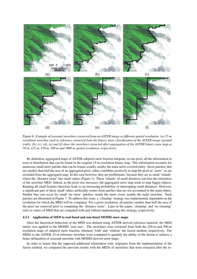
Figure 6: Example of seasonal snowlines extracted from an ASTER image at different spatial resolution. (a) 15-mresolution snowline used as reference extracted from the binary snow classification of the ASTER image (groundtruth); (b), (c), (d), (e) and (f) show the snowlines extracted after aggregation of the ASTER binary snow map at50 m, 125 m, 250 m, 500 m and 1000 m spatial resolution, respectively.

By definition, aggregated maps of ASTER subpixel snow fraction integrate, in one pixel, all the information interm of distribution that can be found in the original 15-m resolution binary map. This information accounts fornumerous small snow patches that can be found, usually, nearby the main snow-covered entity. Snow patches, thatare smaller than half the area of an aggregated pixel, either contribute positively to map the pixel as ‘snow’, or areexcluded from the aggregated map. In this case however, they are problematic, because they act as small ‘islands’where the ‘distance raster’ has small values (Figure 4). These ‘islands’ of small distances can bias the estimationof the snowline MED. Indeed, as the pixel size increases, the aggregated snow map tends to map bigger objects.Keeping all small features therefore leads to an increasing probability of intercepting small distances. However,a significant part of these small values artificially comes from patches that are not accounted in the main object.Similar bias can occur for small ‘no snow’ patches, inside the snow cover, nearby the main snowline. Suchpatches are illustrated in Figure 7. To address this issue, a ‘cleaning’ strategy was implemented, dependent on theresolution for which the MED will be computed. For a given resolution, all patches smaller than half the area ofthe pixel are removed prior to computing the ‘distance raster’. Later in the paper, ‘cleaning’ and ‘no cleaning’refer to values of MED that are computed with and without implementing this strategy, respectively.

4.3.2 Application of MED to real fused and non fused MODIS snow maps

Once the theoretical behaviour of the MED was defined using ASTER derived reference material, the MEDmetric was applied to the MODIS ‘real case’. The snowlines were extracted from both the 250-m and 500-mresolution maps of subpixel snow fraction, obtained ‘with’ and ‘without’ the fusion method, respectively. TheMEDs to the ASTER 15-m reference snowline were computed to quantify the ability of the fusion to achieve abetter delineation of seasonal snowline with MODIS-derived snow maps.

In order to insure that the supposed additional information truly originates from the implementation of thefusion method, we compared the previous results with the MEDs of snowlines that were extracted after the re-

Figure 7: Illustration of the influence of small patches on the determination of snowlines at various spatial resolu-tions. (a) 15-m resolution snowline used as reference extracted from the binary snow classification of the ASTERimage (ground truth); (b), (c), (d), (e) and (f) show the snowlines extracted after aggregation of the ASTER binarysnow map at 50 m, 125 m, 250 m, 500 m and 1000 m spatial resolution, respectively. The ellipses shows snowpatches of different sizes, the circles shows “snow voids” within the main snow entity that can alter the value ofEuclidean distance.

sampling of the 500-m subpixel snow fraction at 250 m resolution using a simple bicubic interpolator.

5 RESULTS AND DISCUSSION5.1 Metric behaviour

An investigation of the behaviour of the metric to different parameters is essential to confirm the relevancy ofthis approach. Initially, we used only the set of reference snowlines extracted at 15 m from ASTER, along withmaps of subpixel snow fraction that were derived by aggregating the binary map at various pixel sizes.

Figure 8 shows the behaviour of the MED of the resulting snowline as a function of the threshold used tosegment the map of subpixel snow fraction. It clearly confirms that, as expected, the shortest average distance isachieved for a snowline created from pixels having more than 50% snow cover. Based on this result, all MED willbe computed after classification of the subpixel snow fraction using the 50% threshold.

Because they are all derived from the same 15-m reference, the ASTER-derived maps of subpixel snow frac-tion, successively aggregated at 50 m, 125 m, 250 m, 500 m and 1000 m, provide the reference dataset to estimatethe sensitivity of the MED to pixel size. Figure 9 shows that the MED significantly increases with the pixelsize, both when cleaning or keeping the smallest snow patches. It confirms our assumption that the snowline isgenerally closer to the reference as the resolution increases, meaning a better match. When computing the MEDwithout the ‘cleaning’ strategy, it is interesting to note that the relationship between the MED and the pixel sizeis not linear. In this case, the dispersion of the MED according to the different dates (see error bars on Figure 9),is significant, suggesting that the metric may be sensitive to the area covered by snow, and eventually the numberof snow patches. However, when applying the ‘cleaning’ strategy, the MED becomes significantly correlated to

Figure 8: Sensitivity of the Mean Euclidean Dis-tance (MED) to the subpixel snow fraction used to bi-nary classifies the snow cover map. For all dates,the ASTER-derived 250-m resolution maps of subpixelsnow fraction were binary classified, with increasingthresholds of subpixel snow fraction. The error barsindicate the standard deviation of the MED for to thefour images.

Figure 9: Sensitivity of the Mean Euclidean Distance(MED) to the aggregation of the binary ASTER-derivedsnow cover map. The error bars indicate the standarddeviation of the MED for to the four images.

the pixel size. The dispersion of the MED between the different dates is also greatly reduced. This confirmsthe significant impact of the small patches in such a multi-scale analysis. Further, when applying the ‘cleaning’strategy the MED consistently drops by 50% when pixel size is reduced by a factor of two. This matches themagnitude of theoretical change that is desirable in the framework of designing an indicator that assesses thequality of a feature as the resolution increases. This validation can be interpreted as a calibration of the metric. Itsets a milestone in terms of what can be expected as an improvement in a real case, for instance by fusing 250-mMODIS bands with 500-m MODIS bands. Simultaneously, the distribution of Euclidean Distances for all samplesalong the whole test snowline also provides a statistical estimation of ‘how far’ it lay from the reality. The meanof the distribution, along with its standard deviation, provides a quantitative insight in terms of the planimetricaccuracy of the snowline position.

5.2 Application to MODIS-derived snow map

Table 1: Mean and standard deviation σ of the Euclidean Distance calculated between the snowline obtained fromMODIS-derived snow maps, and the reference snowline extracted from ASTER at 15 m. ‘Type’ ‘250 m’ refersto the snowline extracted from the MODIS-derived snow map at 250 m resolution obtained with fusion. ‘Type’‘500 m’ refers to the snowline extracted from the MODIS-derived snow map at 500 m resolution obtained withoutfusion. ‘Type’ “interp. 250 m” refers to the snowline extracted after bicubic interpolation at 250 m of the 500-mresolution MODIS-derived snow map.

Date Type Without cleaning With cleaningMED (m) σ (m) MED (m) σ (m)

31/12/2002250 m 31 36 56 58

interp. 250 m 38 43 71 69500 m 44 52 90 87

29/01/2002250 m 56 64 80 95

interp. 250 m 64 65 85 82500 m 76 80 109 107

16/05/2006250 m 80 123 110 155

interp. 250 m 113 146 182 245500 m 102 124 187 241

11/09/2000250 m 76 127 119 263

interp. 250 m 89 112 130 210500 m 103 118 151 209

The results of applying this method to the MODIS dataset are shown in Table 1. For all dates, whether

applying the cleaning strategy or not, the MED values inferred from the 250-m resolution maps using the fusion,are significantly smaller than those derived from the 500-m resolution map. The MED dropped about 26% onaverage (min 22%, max 30%), when not cleaning the smallest snow patches, and about 32% on average (min21%, max 41%) when using the cleaning strategy. This magnitude of improvement must be compared to the 50%improvement that is expected in an ideal case when reducing the pixel size by a factor of two. It suggests that,as expected, the fusion does not achieve what would be obtained if we had real 250-m MODIS-derived snowmap. Nevertheless, the planimetric accuracy of the snowline position has increased of 60% in comparison withthe ASTER reference snowline.

The MED of the snowline obtained from the interpolated map improved 8% and 15% without and with thecleaning strategy, respectively. This improvement was expected since the interpolation process was likely to movethe snowline towards the reference due to the correlation of the subpixel snow fraction in space. Nevertheless, therange of improvement is still half what was achieved with the fusion. This comparison suggests that the fusionadds significantly more information, with regard to the accuracy of snow distribution, than a simple interpolation.

The MED is higher for the two winter images than the summer one, suggesting that the classification is moreaccurate in summer. The presence of stronger shadow effects, along with a larger snow extent in winter images,is expected to increase the noise in the process of retrieving the subpixel snow fraction. The lower quality for thewinter images is consistent with what was previously observed by Sirguey et al. (2008).

6 CONCLUSIONThe Mean Euclidean Distance (MED) has been investigated as a relevant metric to objectively assess the

improvement of the snow mapping process, following an increase of the spatial resolution of MODIS bands usingimage fusion. In this study, we assumed that in the case of a binary segmentation of the image, the quality of theclassification can be assessed by an estimation of how well the boundary between the two classes ‘snow’ and ‘nosnow’ matches the reality.

The sensitivity of the MED to the spatial resolution was investigated using reference images obtained fromASTER and proved the MED to be suitable to objectively quantify such match or discrepancy. The metric alsorevealed objectively that in the case of a continuous classification of subpixel snow fraction, the 50% snow coveredlimit is the optimum threshold to depict the snowline. Our investigation of a real case involving fusion appliedto MODIS imagery, showed that: (1) The MED of the 250-m resolution snow map, obtained with the fusion,was significantly lower than the MED of the 500-m snow map. The 32% decrease of the MED means the fusionprovided 64% of the accuracy improvement that could ideally be achieved, if we had real 250-m resolution bands;and (2) although a significant improvement in terms of MED can be achieved by a simple interpolation of the500-m resolution snow map to 250 m resolution, the interpolation clearly failed to depict as much information asthe fusion. We suggest that this metric can be useful to assess the performance of image fusion, along with otherprotocols, such as visual interpretation and pixel-based image quality assessment, but with the advantage of beingcomparable at all resolutions.

In addition, the investigation of the distribution of Euclidean Distance, between a class boundary and a cor-responding reference, also provides a comprehensive and useful insight with regard to the planimetric accuracyof class boundaries. Although, in this study, the MED indicator has been designed for binary classification ofsnow, it can be suitable to assess the quality of various natural pattern outlines. In the case of more classes, theuse of this indicator in a more sophisticated strategy can be investigated, to both assess the position of boundariesand the correct classification of the objects on each side of the boundary. However, it is obviously important toaddress the issue raised by small patches that can bias the metric, and modify its linear behaviour according to theresolution.

ReferencesAiazzi, B., Alparone, L., Argenti, F. & Baronti, S. (1999). “Wavelet and pyramid techniques for multisensor data

fusion: a performance comparison varying with scale ratios” In S. B. Serpico (ed.), Proceedings of the SPIEImage Signal Process. For Remote Sensing V. Vol. 3871 SPIE SPIE. pp. 251–262.

Alparone, L., Baronti, S., Garzelli, A. & Nencini, F. (2004). “A global quality measurement of pan-sharpenedmultispectral imagery” IEEE Geoscience and Remote Sensing Letters. 1(4): 313–317.

Alparone, L., Wald, L., Chanussot, J., Thomas, Gamba, P. & Bruce, L. M. (2007). “Comparison of pansharpeningalgorithms: outcome of the 2006 GRS-S data fusion contest” IEEE Transactions on Geoscience and RemoteSensing. 45(10): 3012–3021.

Amolins, K., Zhang, Y. & Dare, P. (2007). “Wavelet based image fusion techniques – An introduction, reviewand comparison” Journal of Photogrammetry and Remote Sensing. 62(4): 249–263.

Bendjoudi, H. (2002). “The gravelius compactness coefficient: critical analysis of a shape index for drainagebasins” Hydrological Sciences Journal. 47(6): 921–930.

Chen, H. & Varshney, P. K. (2007). “A human perception inspired quality metric for image fusion based onregional information” Information Fusion. 8(2): 193–207.

Crane, R. G. & Anderson, M. R. (1984). “Satellite discrimination of snow / cloud surfaces” International Journalof Remote Sensing. 5: 213–223.

Du, Y., Vachon, P. W. & van der Sanden, J. J. (2003). “Satellite image fusion with multiscale wavelet analysis formarine applications: preserving spatial information and minimizing artifacts (PSIMA)” Canadian Journal ofRemote Sensing. 29(1): 14–23.

Gao, X., Wang, T. & Li, J. (2005). “A content-based image quality metric” Lecture Notes in Computer Science.3642: 231–240. to get.

Garguet-Duport, B., Girel, J., Chassery, J.-M. & Pautou, G. (1996). “The use of multi-resolution analysis andwavelet transform for merging SPOT panchromatic and multispectral imagery data” Photogrammetric Engi-neering and Remote Sensing. 62(9): 1057–1066.

Gonzalez-Audicana, M., Otazu, X., Fors, O. & Alvarez-Mozos, J. (2006). “A low computational-cost method tofuse IKONOS images using the spectral response function of its sensors” IEEE Transactions on Geoscienceand Remote Sensing. 44(6): 1683–1691.

Gonzalez-Audicana, M., Saleta, J. L., Catalan, R. G. & Garcıa, R. (2004). “Fusion of multispectral and panchro-matic images using improved IHS and PCA mergers based on wavelet decomposition” IEEE Transactions onGeoscience and Remote Sensing. 42(6): 1291–1299.

Goodchild, M. (1980). “Fractals and the accuracy of geographical measures” Mathematical Geology. 12(2): 85–98.

Goodchild, M. F. & Mark, D. M. (1987). “The fractal nature of geographic phenomena” Annals of Association ofAmerican Geographers. 77(2): 265–278.

Jin, X. Y. & Davis, C. H. (2005). “Automated building extraction from high-resolution satellite imagery in urbanareas using structural, contextual, and spectral information” EURASIP Journal of Applied Signal Processing.2005(14): 2196–2206.

Keshava, N. (2003). “A survey of spectral unmixing algorithms” Lincoln Laboratory Journal. 14(1): 55–78.

Lam, N. S.-N. & Quattrochi, D. A. (1992). “On the issues of scale, resolution, and fractal analysis in the mappingsciences” Professional Geographer. 44(1): 88–98.

Laporterie-Dejean, F., de Boissezon, H., Flouzat, G. & Lefevre-Fonollosa, M.-J. (2005). “Thematic and sta-tistical evaluations of five panchromatic/multispectral fusion methods on simulated PLEIADES-HR images”Information Fusion. 6(3): 193–212.

Lasaponara, R. & Masini, N. (2005). “QuickBird-based analysis for the spatial characterization of archaeologicalsites: case study of the Monte Serico medieval village” Geophysical Research Letter. 32(12): L12313.

Li, X., He, H. S., Bu, R., Wen, Q., Chang, Y., Hu, Y. & Li, Y. (2005). “The adequacy of different landscapemetrics for various landscape patterns” Pattern Recognition. 38(12): 2626–2638.

Malpica, J. A. (2007). “Hue adjustment to IHS pan-sharpened IKONOS imagery for vegetation enhancement”IEEE Geoscience and Remote Sensing Letters. 4(1): 27–31.

Nichol, J. & Wong, M. S. (2005). “Satellite remote sensing for detailed landslide inventories using changedetection and image fusion” International Journal of Remote Sensing. 26(9): 1913–1926.

Pasqualini, V., Pergent-Martini, C., Pergent, G., Agreil, M., Skoufas, G., Sourbes, L. & Tsirika, A. (2005). “Useof SPOT 5 for mapping seagrasses: An application to Posidonia oceanica” Remote Sensing of Environment.94(1): 39–45.

Petrovic, V. (2007). “Subjective tests for image fusion evaluation and objective metric validation” InformationFusion. 8(2): 208–216.

Pohl, C. & Genderen, J. L. V. (1998). “Multisensor image fusion in remote sensing: concepts, methods andapplications” International Journal of Remote Sensing. 19(5): 823–854.

Ranchin, T., Aiazzi, B., Alparone, L., Baronti, S. & Wald, L. (2003). “Image fusion–the ARSIS concept and somesuccessful implementation schemes” Journal of Photogrammetry and Remote Sensing. 58: 4–18.

Ranchin, T. & Wald, L. (2000). “Fusion of high spatial and spectral resolution images : the ARSIS concept andits implementation” Photogrammetric Engineering and Remote Sensing. 66(1): 49–61.

Richter, R. (1998). “Correction of satellite imagery over mountainous terrain” Applied Optics. 37(18): 4004–4015.

Shi, W., Zhu, C., Tian, Y. & Nichol, J. (2005). “Wavelet-based image fusion and quality assessment” InternationalJournal of Applied Earth Observation and Geoinformation. 6: 241–251.

Sirguey, P., Mathieu, R., Arnaud, Y., Khan, M. M. & Chanussot, J. (2008). “Improving MODIS spatial resolutionfor snow mapping using wavelet fusion and ARSIS concept” IEEE Geoscience and Remote Sensing Letters.5(1): doi:10.1109/LGRS.2007.908884. In Press.

Toet, A. & Franken, E. M. (2003). “Perceptual evaluation of different image fusion schemes” Displays. 24(1): 25–37.

Tu, T.-M., Huang, P. S., Hung, C.-L. & Chang, C.-P. (2004). “A fast Intensity–Hue–Saturation fusion techniquewith spectral adjustment for IKONOS imagery” IEEE Geoscience and Remote Sensing Letters. 1(4): 309–312.

Wald, L. (2000). “Quality of high resolution synthesized images: is there a simple criterion?” Proceedings of theInternational Conference on Fusion of Earth Data. SEE Greca Sophia Antipolis, France pp. 99–105.

Wald, L., Ranchin, T. & Mangolini, M. (1997). “Fusion of satellite images of different spatial resolution: assessingthe quality of resulting images” Photogrammetric Engineering and Remote Sensing. 63(6): 691–699.

Wang, Z. & Bovik, A. C. (2002). “A universal image quality index” IEEE Signal Processing Letters. 9(3): 81–84.

Woodcock, C. E. & Strahler, A. H. (1987). “The factor of scale in remote sensing” Remote Sensing of Environment.21(3): 311–332.

Xydeas, C. S. & Petrovic, V. (2000). “Objective image fusion performance measure” Electronics Letters.36(4): 308–309.

Zhai, G., Zhang, W., Yang, X. & Xu, Y. (2005). “Image quality assessment metrics based on multi-scale edgepresentation” Proceedings of the IEEE Workshop on Signal Processing Systems Design and Implementation.IEEE IEEE. pp. 331–336.

Zhan, Q., Molenaar, M., Tempfli, K. & Shi, W. (2005). “Quality assessment for geo-spatial objects derived fromremotely sensed data” International Journal of Remote Sensing. 26(14): 2953–2974.

Zhang, W. J. & Kang, J. Y. (2006). “QuickBird panchromatic and multi-spectral image fusion using waveletpacket transform” Intelligent Control and Automation. 344: 976–981.

Zhang, Y. (2004). “Understanding image fusion” Photogrammetric Engineering and Remote Sensing. 70(6): 657–661.