Embed Size (px)
Citation preview
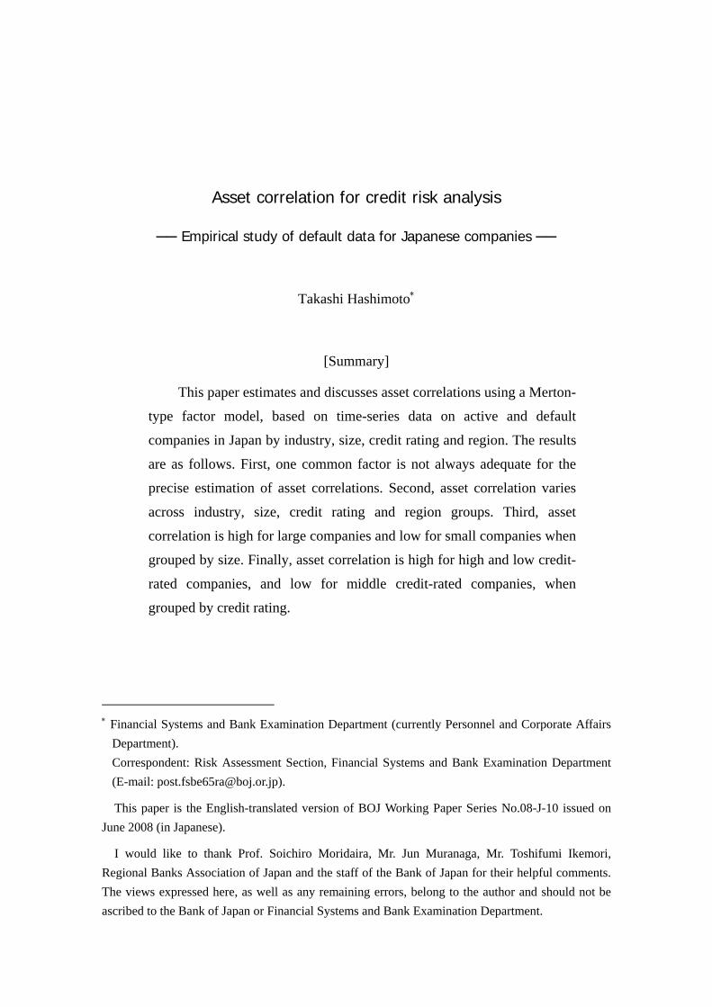
No.09-E-3 August 2009
Asset correlation for credit risk analysis -Empirical study of default data for Japanese companies- Takashi Hashimoto* Bank of Japan 2-1-1 Nihonbashi-Hongokucho, Chuo-ku, Tokyo 103-8660, Japan
* Financial Systems and Bank Examination Department(currently Personnel and Corporate Affairs Department)
Papers in the Bank of Japan Working Paper Series are circulated in order to stimulate discussion and comments. Views expressed are those of authors and do not necessarily reflect those of the Bank. If you have any comment or question on the working paper series, please contact each author. When making a copy or reproduction of the content for commercial purposes, please contact the Public Relations Department ([email protected]) at the Bank in advance to request permission. When making a copy or reproduction, the source, Bank of Japan Working Paper Series, should explicitly be credited.
Bank of Japan Working Paper Series
Asset correlation for credit risk analysis
── Empirical study of default data for Japanese companies ──
Takashi Hashimoto∗
[Summary]
This paper estimates and discusses asset correlations using a Merton-
type factor model, based on time-series data on active and default
companies in Japan by industry, size, credit rating and region. The results
are as follows. First, one common factor is not always adequate for the
precise estimation of asset correlations. Second, asset correlation varies
across industry, size, credit rating and region groups. Third, asset
correlation is high for large companies and low for small companies when
grouped by size. Finally, asset correlation is high for high and low credit-
rated companies, and low for middle credit-rated companies, when
grouped by credit rating.
∗ Financial Systems and Bank Examination Department (currently Personnel and Corporate Affairs
Department). Correspondent: Risk Assessment Section, Financial Systems and Bank Examination Department (E-mail: [email protected]).
This paper is the English-translated version of BOJ Working Paper Series No.08-J-10 issued on June 2008 (in Japanese).
I would like to thank Prof. Soichiro Moridaira, Mr. Jun Muranaga, Mr. Toshifumi Ikemori, Regional Banks Association of Japan and the staff of the Bank of Japan for their helpful comments. The views expressed here, as well as any remaining errors, belong to the author and should not be ascribed to the Bank of Japan or Financial Systems and Bank Examination Department.

Table of Contents
1. Introduction 1
2. One-factor Merton model 2
(1) Single Index Model 3
(2) Multi Index Model 3
3. Estimating the asset correlations 3
(1) Reasons for selecting Multi Index Model 5
(2) Grouping criteria and asset correlation 7
I. Industry 7
II. Company size 9
III. Credit rating 12
IV. Region 15
4. Conclusion 18
Appendix 1. Single-factor model 20
Appendix 2. Summary of previous studies of asset correlation estimation 26
Appendix 3. Estimation methods and differences in results 29
Appendix 4. The number of data for estimation of asset correlation 36
References 38
1
1. Introduction
Financial institutions need to manage their credit risks to make a profit. In Japan,
many financial institutions use an internal rating system to control their loans. In
addition, they evaluate the quality of their portfolio using the Expected Loss (EL) and
the Unexpected Loss (UL). When financial institutions calculate the UL, they often use
a Merton model that requires setting up the following parameters: Probability of Default
(PD), Loss Given Default (LGD), Exposure at Default (EaD) and Asset Correlation
(AC). AC represents asset correlation of exposures to multiple debtors when they
default simultaneously. Following the introduction of Basel II, they have been required
to estimate the PD, LGD and EaD. However, estimation of the AC, which is not
required for estimations associated with Pillar I of Basel II, has not often been discussed,
even though it substantially affects the estimates of the UL. Importantly, it is essential
that financial institutions use the appropriate method and data to calculate the AC in
order to compute the UL accurately.
Theoretically, we can define the asset correlation for each loan. Generally, however,
it is difficult to estimate all asset correlations of each loan because we cannot observe
the value of each loan in the market and because financial institutions usually lend
money to a large number of companies (borrowers). Therefore, in their risk analysis,
financial institutions sum up loans by each company. Specifically, when they estimate
asset correlations, they often construct groups of companies using a certain rule and
estimate the asset correlation for each group. This rule is a key factor in estimating asset
correlations and is essential for calculating the UL correctly. In this paper, we present
several types of rules used to construct groups and compare the results of the asset
correlations obtained.
In our analysis, we use the Teikoku Data Bank’s Matrix Data (1985–2005) to
estimate the asset correlations for each group, because these data provide historical
default data for Japanese companies. Using this data, we calculate the default rate for
each year and group.
The structure of the paper is as follows. Section 2 presents the Merton Model used
in the analysis. Section 3 provides the estimations. Section 4 discusses the results and
draws conclusions.
2
2. One-factor Merton model
We estimate asset correlations using default data on Japanese companies. We use a
one-factor Merton model1 as it is an important model to calculate credit risk, not only in
Japan but also elsewhere, because of its inclusion in the calculation of the capital
adequacy requirements in Basel II.
The one-factor Merton model describes a company’s value with a systematic factor
(a factor common to the values of several companies) and an idiosyncratic factor (a
factor specific to the company’s value). The asset value of a company is then the
weighted sum of a common (systematic) factor and an individual (idiosyncratic) factor.
For example, when the macroeconomic development can be regarded as the systematic
factor, the asset value of the company can be explained by the macroeconomic
development and the company’s individual factor. When these two factors change over
time, the asset value of the company also changes.
In the Merton model, the occurrence of default is regarded as the time when the
company’s value is below a certain threshold at the time of maturity.
In this paper, we classify companies into several groups using a number of criteria
(industry, size, credit and region)2, and calculate the asset correlation for each group.
We refer to the model that sets a common systematic factor for all companies as the
Single Index Model and the model that sets a different systematic factor for each group
of companies as the Multi Index Model. In this analysis, we mainly use the Multi Index
Model.
1 See Appendix 1 for details of the single-factor model. See footnote 22 in Appendix 1 for details of the
multifactor model. 2 For example, when we use “industry” as a criterion, we can make groups of “Manufacturing”,
“Construction”, and “Service”. As another example, when we use “company size” as a criterion, we can make groups of “Large companies”, “Small companies” and “Personal companies” (see footnote 11 for details of the definition of company size).
3
(1) Single Index Model
In the Single Index Model, the value )(tZi of company ia belonging to group kS
is:
)(1)()( ttXtZ ikki ερρ −+=
10 ≤≤ kρ , ki Sa ∈ , ni ,...,2,1= , mk ,...,2,1=
where time t ( 0≥t ), n is the number of companies and m is the number of groups.
The value iZ of company ia is described by two independent random variables: a
systematic factor )(tX (the factor common to all companies) and an idiosyncratic factor
)(tiε (the factor specific to company ia ). The companies that belong to group kS have
the same asset correlation or kρ , and kρ indicates the sensitivity of the company’s
value )(tZi to the systematic factor )(tX . We assume )(tX and )(tiε follow a standard
normal distribution independently of each other, meaning that )(tX and )(tiε are i.i.d.
(independent and identically distributed). Therefore, )(tZi also follows a standard
normal distribution because )(tZi is a linear combination of )(tX and )(tiε .
(2) Multi Index Model
In the Multi Index Model, the value )(tZi of company ia belonging to group kS is:
)(1)()( ttXtZ ikkki ερρ −+=
10 ≤≤ kρ , ki Sa ∈ , ni ,...,2,1= , mk ,...,2,1=
at time t ( 0≥t ). When we establish )(tZi in the Single Index Model, we use the
systematic factor )(tX , which takes the same value for all companies. Conversely, in
the Multi Index Model, we use the systematic factor )(tX k , which takes different
values for each kS 3.
3. Estimating the asset correlations
In this section, we estimate the asset correlations using the Teikoku Data Bank’s
Matrix Data for calculating default rate. This database tracks Japanese company data
3 See Appendix 1(3) for details.
4
from 1985 to 2005 and currently covers about 1.2 million companies.
To start with, we confirm the necessity to employ the Multi Index Model to
calculate the UL. We then estimate the asset correlations for four groups: (1) industry
type, (2) company size, (3) credit rating (the Teikoku Data Bank Score4), and (4) region.
We use these particular groupings because analysts often use these criteria in credit risk
management and because several previous studies use the same criteria5.
Figure 1 depicts the time series of the total number of companies6 and the number of
default companies7 in the database.
4 The webpage of Teikoku Data Bank (in Japanese) describes the Score as follows: “The Teikoku Data
Bank Score means how Teikoku Data Bank evaluates the company. The full score is 100. Teikoku Data Bank evaluates, as a third party, whether the company is well managed, is solvent and is able to deal with other companies safely.”
5 See Appendix 2 for details of previous studies. 6 In this paper, we use company data included in the Teikoku Data Bank’s Matrix Data, of which scores of
the previous year end were given by the Teikoku Data Bank. We do not include company data for which Teikoku Data Bank shows “no score”.
7 In this paper, we define default as any of the following definitions of bankruptcy given by Teikoku Data Bank: (1) drawing unpaid notes twice and transactions with banks are suspended; (2) dissolution of the company (when the representative declares bankruptcy); (3) applying to the court for the application of the Corporate Rehabilitation Law; (4) applying to the court for the commencement of procedures based on the Civil Rehabilitation Law; (5) applying to the court for liquidation; and (6) applying to the court for the commencement of special liquidation.
5
[Figure 1] The number of companies and default companies in the database
(left axis: thousands of companies; right axis: number of companies)
0
2,000
4,000
6,000
8,000
10,000
12,000
14,000
0
200
400
600
800
1,000
1,200
1,400 19
8519
8619
8719
8819
8919
9019
9119
9219
9319
9419
9519
9619
9719
9819
9920
0020
0120
0220
0320
0420
05
The number of companies(left axis)
The number of default companies(right axis)
(1) Reasons for using the Multi Index Model
We use the Multi Index Model with Maximum Likelihood Estimation 8 , 9 when
estimating the asset correlation. In this section, we describe why we use the Multi Index
Model rather than the Single Index Model.
Figure 2 depicts the cumulative R-squared values of the principal component
analysis using the time-series default rate data by industry type, company size, credit
rating and region. Figure 2 shows that while the values of R-squared for the first
component are low in all cases, the cumulative values of R-squared for the first and
second components are more than 90 percent in most cases. This means that it is
difficult to explain the changes in default rates only by the first component.
8 See Appendix 3 for details of the Maximum Likelihood Estimation and Method of Moments and a
comparison of the results. 9 We use MATLAB for the calculations. For the integral calculus in formula (15) in Appendix 3, we use
quasi Monte Carlo integration by Halton sequence (the number of random variables is 216 – 1 = 65,535).
6
[Figure 2] Cumulative values of R-squared
50%
60%
70%
80%
90%
100%
industry company size credit rating region
First component Second component Third component
This result shows that analysts must take into consideration both of the first and the
second components. Figure 3 depicts the component loading for each type of industry.
[Figure 3] Component loading for each industry type
-1
-0.8
-0.6
-0.4
-0.2
0
0.2
0.4
0.6
0.8
1
Agric
ultu
re, f
ores
try,
hun
ting,
fish
ery
and
min
ing Co
nstr
uctio
n
Man
ufac
turin
g
Reta
il, w
hole
sale
, res
taur
ant
Fina
nce
Real
est
ate
com
pany
Tran
spor
tatio
n, te
leco
mm
unic
atio
ns,
elec
tric
ity, g
as, e
tc.
Serv
ice
First Component
Second Component
7
In Figure 3, the first component shows the common factor for all industry types but
the second component does not. As shown, the first component displays the same sign
for every industry type, while the second component has a different sign for each type
of industry. In all types of industry, except finance and real estate, the common factor
explains most of the change in default rate because the first component is larger than the
second component. In contrast, in finance and real estate, the common factor cannot
explain changes in the default rate because the second component is also large.
From this analysis, we conclude that a common factor alone cannot describe the
asset value of companies because the values of R-squared for the time series of default
rates indicate that finance and real estate display different results from other industries.
Therefore, this paper proposes the following two-factor model, which contains not only
an individual factor and a common factor but also a common group factor:
)(1)()()( 22 tttXtZ ikkkkki εβαδβα −−++=
10 ≤≤ kρ , ki Sa ∈ , ni ,...,2,1= , mk ,...,2,1=
This formula contains not only )(tX (the factor common to all companies) and )(tiε
(the individual factor for company ia ), but also )(tkδ (the factor common to group kS
that includes company ia ), where kα and kβ are the asset correlations in a two-factor
model. We set ρρα kk = and 21 ρρβ −= kk and rewrite the above as:
)(1))(1)((
)(1)(1)()(
tttX
tttXtZ
ikkk
ikkkki
ερδρρρ
ερδρρρρ
−+−+=
−+−+=.
We then set )()(1)( tXttX kk =−+ δρρ ,
)(1)()( ttXtZ ikkki ερρ −+= .
This is the same formula as in the Multi Index Model. For simplification, we apply in
this paper the Multi Index Model that focuses on the estimation and analysis of the
value of kρ .
(2) Grouping criteria and asset correlation
I. Industry
We group the Teikoku Data Bank’s Matrix Data by industry type. Table 1 shows the
categorization of the eight industry groups in this paper. Note that, because
8
“agriculture”, “forestry and hunting”, “fishery” and “mining” include so few companies
individually, we include these as a single industry, “agriculture, forest, hunting, fishery
and mining”. Note also that because the number of default companies in the “electricity,
gas, water and heat supplier” industry is small, we combine it with the “transportation
and telecommunications” industries into a composite group “transportation,
telecommunications, electricity, gas, etc.”10
[Table 1] Industry groups Industry groups in this paper Major industry groups in the Teikoku Data
Bank’s Matrix Data 1 Agriculture, forestry, hunting,
fishery and mining “Agriculture” + “Forestry and hunting” + “Fishery” + “Mining”
2 Construction “Construction” 3 Manufacturing “Manufacturing” 4 Retail wholesale, restaurant “Retail and wholesale, restaurant” 5 Finance “Finance” 6 Real estate “Real estate” 7 Transportation, telecommunications,
electricity, gas, etc. “Electricity, gas, water and heat supplier” + “Transportation and telecommunications”
8 Service “Service”
Figure 4 plots the transition of the default rate for each industry.
[Figure 4] Transition of default rate in each industry
0.0%
0.5%
1.0%
1.5%
2.0%
2.5%
1985
1986
1987
1988
1989
1990
1991
1992
1993
1994
1995
1996
1997
1998
1999
2000
2001
2002
2003
2004
2005
Agriculture, forestry, hunting, fishery and mining
Construction
Manufacturing
Retail, wholesale, restaurant
Finance
Real estate
Transportation, telecommunications, electricity, gas, etc.
Service
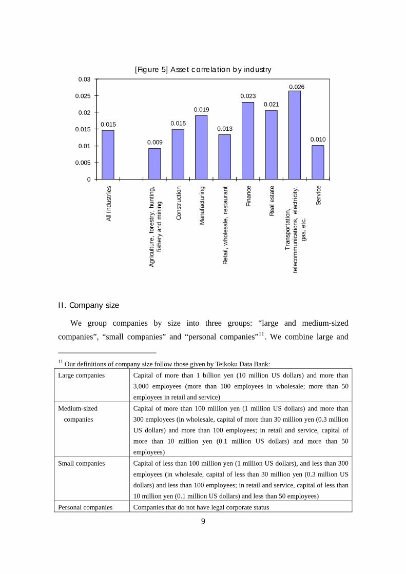
Figure 5 provides an estimate of the asset correlation for each industry. The data we
use are the default status of the companies at the beginning of and during the term. As
shown, the asset correlation differs across various industries.
10 See appendix 4 for the number of companies and the number of default companies for each group.
9
[Figure 5] Asset correlation by industry
0.015
0.009
0.015
0.019
0.013
0.0230.021
0.026
0.010
0
0.005
0.01
0.015
0.02
0.025
0.03
All I
ndus
trie
s
Agric
ultu
re,
fore
stry
, hun
ting,
fis
hery
and
min
ing
Cons
truc
tion
Man
ufac
turin
g
Reta
il, w
hole
sale
, re
stau
rant
Fina
nce
Real
est
ate
Tran
spor
tatio
n,
tele
com
mun
icat
ions
, el
ectr
icity
, ga
s, e
tc.
Serv
ice
II. Company size
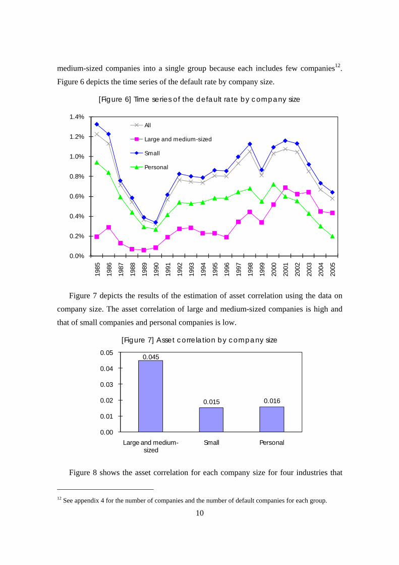
We group companies by size into three groups: “large and medium-sized
companies”, “small companies” and “personal companies”11. We combine large and
11 Our definitions of company size follow those given by Teikoku Data Bank:
Large companies Capital of more than 1 billion yen (10 million US dollars) and more than 3,000 employees (more than 100 employees in wholesale; more than 50 employees in retail and service)
Medium-sized companies
Capital of more than 100 million yen (1 million US dollars) and more than 300 employees (in wholesale, capital of more than 30 million yen (0.3 million US dollars) and more than 100 employees; in retail and service, capital of more than 10 million yen (0.1 million US dollars) and more than 50 employees)
Small companies Capital of less than 100 million yen (1 million US dollars), and less than 300 employees (in wholesale, capital of less than 30 million yen (0.3 million US dollars) and less than 100 employees; in retail and service, capital of less than 10 million yen (0.1 million US dollars) and less than 50 employees)
Personal companies Companies that do not have legal corporate status
10
medium-sized companies into a single group because each includes few companies12.
Figure 6 depicts the time series of the default rate by company size.
[Figure 6] Time series of the default rate by company size
0.0%
0.2%
0.4%
0.6%
0.8%
1.0%
1.2%
1.4%
1985
1986
1987
1988
1989
1990
1991
1992
1993
1994
1995
1996
1997
1998
1999
2000
2001
2002
2003
2004
2005
All
Large and medium-sized
Small
Personal
Figure 7 depicts the results of the estimation of asset correlation using the data on
company size. The asset correlation of large and medium-sized companies is high and
that of small companies and personal companies is low.
[Figure 7] Asset correlation by company size
0.045
0.015 0.016
0.00
0.01
0.02
0.03
0.04
0.05
Large and medium-sized
Small Personal
Figure 8 shows the asset correlation for each company size for four industries that
12 See appendix 4 for the number of companies and the number of default companies for each group.
11
has a large number of companies. Similar to Figure 7, Figure 8 shows that asset
correlation is high in large and medium-sized companies and low in small companies
and personal companies.
[Figure 8] Asset correlation by company size for major industries
0.053 0.050
0.057
0.032
0.020 0.023
0.012 0.010 0.016
0.024
0.013 0.012
0.00
0.01
0.02
0.03
0.04
0.05
0.06
0.07 M
anuf
actu
ring
Cons
truc
tion
Ret
ail,
who
lesa
le,
rest
aura
nt
Serv
ice
Large and medium-sized
Small
Personal
Literature survey13 shows that, Düllmann and Scheule [2003], Lopez [2004] and
Kitano [2007] argued that the smaller the size of the company, the lower the asset
correlation14. Our findings are consistent with these previous studies. This could be
attributed to the following hypotheses. First, the asset correlation of large companies is
high because the performance of large companies is similar to the economic system—
for example, the economic situation for a company in the particular region or industry to
which the company belongs—and so large companies are affected by the systematic
factor more than by the idiosyncratic factor. Second, the asset correlation of small
companies and personal companies is lower because individual factors affect small
companies more than the economic system does.
13 See Appendix 2. 14 Dietsch and Petey [2004] show that the shape of the asset correlation function is convex downward in
terms of company size (the amount of sales). We explain this point further in Section 3, (2), III. Credit rating.
12
0%
1%
2%
3%
4%
5%
6%
7%
1985
1986
1987
1988
1989
1990
1991
1992
1993
1994
1995
1996
1997
1998
1999
2000
2001
2002
2003
2004
2005
26-30
31-35
36-40
41-45
46-50
51-55
56-60
61-65
66-70
71-75
76-80
III. Credit rating
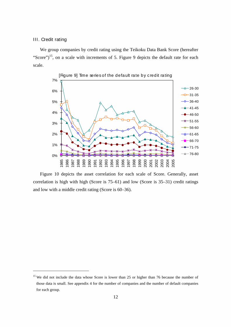
We group companies by credit rating using the Teikoku Data Bank Score (hereafter
“Score”)15, on a scale with increments of 5. Figure 9 depicts the default rate for each
scale.
[Figure 9] Time series of the default rate by credit rating
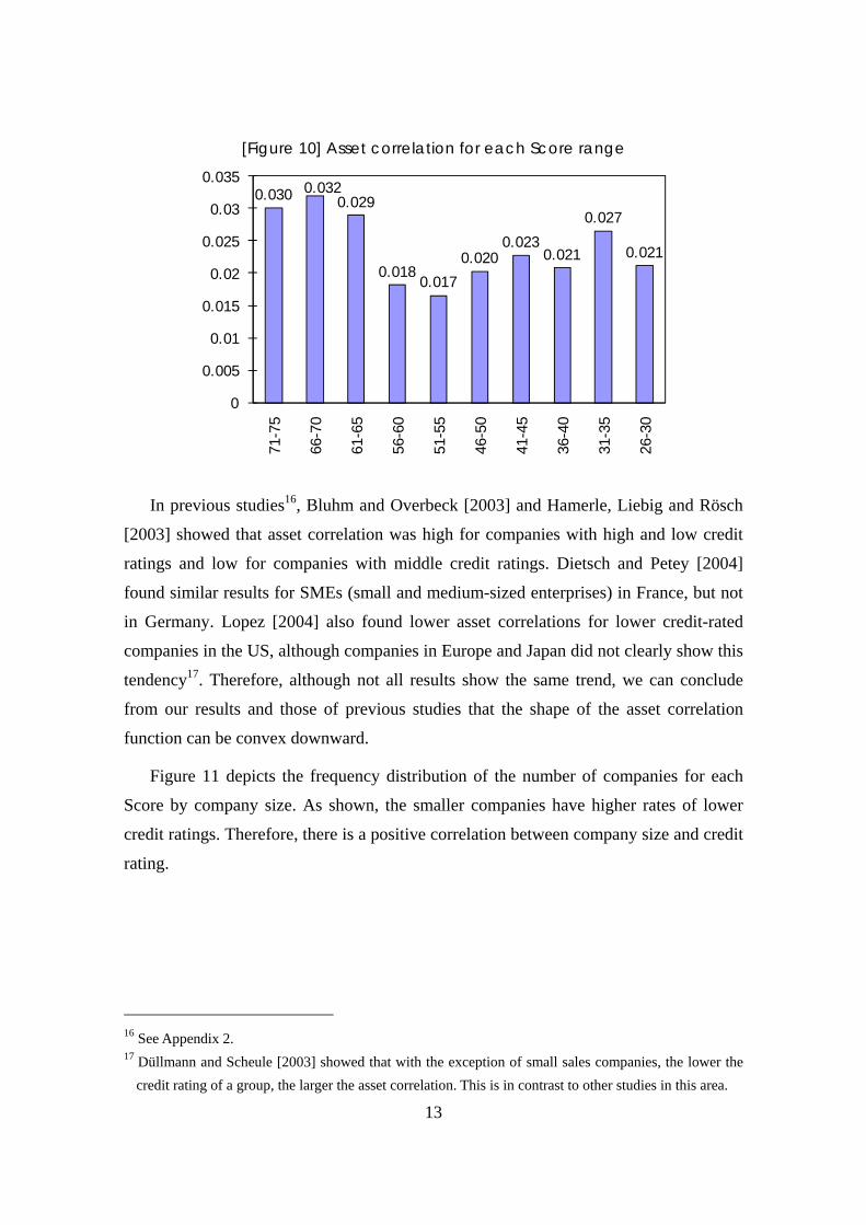
Figure 10 depicts the asset correlation for each scale of Score. Generally, asset
correlation is high with high (Score is 75–61) and low (Score is 35–31) credit ratings
and low with a middle credit rating (Score is 60–36).
15 We did not include the data whose Score is lower than 25 or higher than 76 because the number of
those data is small. See appendix 4 for the number of companies and the number of default companies for each group.
13
[Figure 10] Asset correlation for each Score range
0.030 0.032 0.029
0.018 0.017
0.020 0.023
0.021
0.027
0.021
0
0.005
0.01
0.015
0.02
0.025
0.03
0.035
71-7
5
66-7
0
61-6
5
56-6
0
51-5
5
46-5
0
41-4
5
36-4
0
31-3
5
26-3
0
In previous studies16, Bluhm and Overbeck [2003] and Hamerle, Liebig and Rösch
[2003] showed that asset correlation was high for companies with high and low credit
ratings and low for companies with middle credit ratings. Dietsch and Petey [2004]
found similar results for SMEs (small and medium-sized enterprises) in France, but not
in Germany. Lopez [2004] also found lower asset correlations for lower credit-rated
companies in the US, although companies in Europe and Japan did not clearly show this
tendency17. Therefore, although not all results show the same trend, we can conclude
from our results and those of previous studies that the shape of the asset correlation
function can be convex downward.
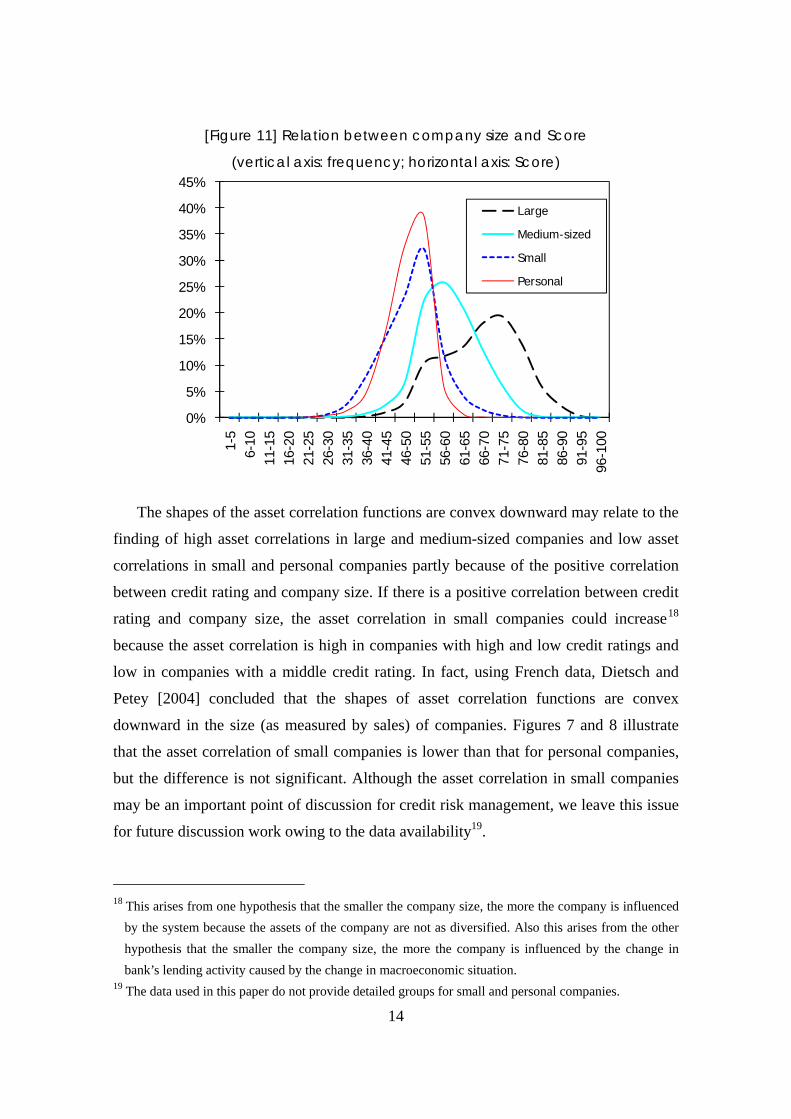
Figure 11 depicts the frequency distribution of the number of companies for each
Score by company size. As shown, the smaller companies have higher rates of lower
credit ratings. Therefore, there is a positive correlation between company size and credit
rating.
16 See Appendix 2. 17 Düllmann and Scheule [2003] showed that with the exception of small sales companies, the lower the
credit rating of a group, the larger the asset correlation. This is in contrast to other studies in this area.
14
[Figure 11] Relation between company size and Score
(vertical axis: frequency; horizontal axis: Score)
0%
5%
10%
15%
20%
25%
30%
35%
40%
45%
1-5
6-10
11-1
516
-20
21-2
526
-30
31-3
536
-40
41-4
546
-50
51-5
556
-60
61-6
566
-70
71-7
576
-80
81-8
586
-90
91-9
596
-100
Large
Medium-sized
Small
Personal
The shapes of the asset correlation functions are convex downward may relate to the
finding of high asset correlations in large and medium-sized companies and low asset
correlations in small and personal companies partly because of the positive correlation
between credit rating and company size. If there is a positive correlation between credit
rating and company size, the asset correlation in small companies could increase18
because the asset correlation is high in companies with high and low credit ratings and
low in companies with a middle credit rating. In fact, using French data, Dietsch and
Petey [2004] concluded that the shapes of asset correlation functions are convex
downward in the size (as measured by sales) of companies. Figures 7 and 8 illustrate
that the asset correlation of small companies is lower than that for personal companies,
but the difference is not significant. Although the asset correlation in small companies
may be an important point of discussion for credit risk management, we leave this issue
for future discussion work owing to the data availability19.
18 This arises from one hypothesis that the smaller the company size, the more the company is influenced
by the system because the assets of the company are not as diversified. Also this arises from the other hypothesis that the smaller the company size, the more the company is influenced by the change in bank’s lending activity caused by the change in macroeconomic situation.
19 The data used in this paper do not provide detailed groups for small and personal companies.
15
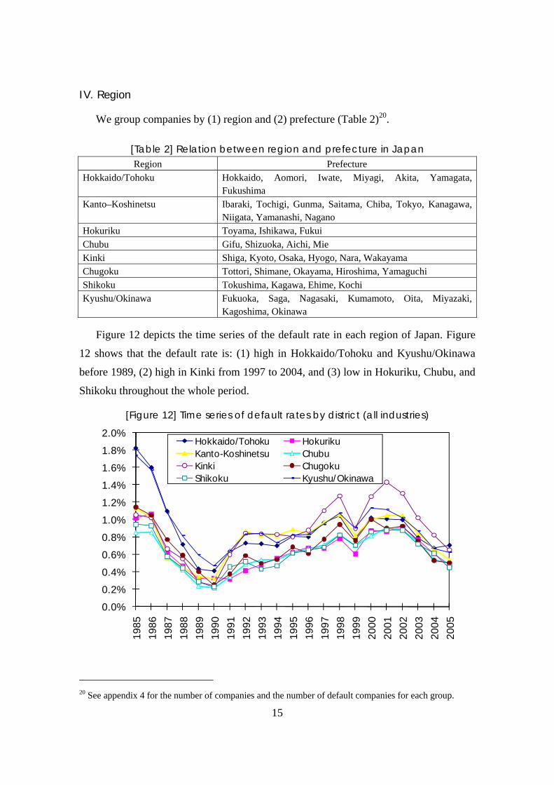
IV. Region
We group companies by (1) region and (2) prefecture (Table 2)20.
[Table 2] Relation between region and prefecture in Japan Region Prefecture
Hokkaido/Tohoku Hokkaido, Aomori, Iwate, Miyagi, Akita, Yamagata, Fukushima
Kanto–Koshinetsu Ibaraki, Tochigi, Gunma, Saitama, Chiba, Tokyo, Kanagawa, Niigata, Yamanashi, Nagano
Hokuriku Toyama, Ishikawa, Fukui Chubu Gifu, Shizuoka, Aichi, Mie Kinki Shiga, Kyoto, Osaka, Hyogo, Nara, Wakayama Chugoku Tottori, Shimane, Okayama, Hiroshima, Yamaguchi Shikoku Tokushima, Kagawa, Ehime, Kochi Kyushu/Okinawa Fukuoka, Saga, Nagasaki, Kumamoto, Oita, Miyazaki,
Kagoshima, Okinawa
Figure 12 depicts the time series of the default rate in each region of Japan. Figure
12 shows that the default rate is: (1) high in Hokkaido/Tohoku and Kyushu/Okinawa
before 1989, (2) high in Kinki from 1997 to 2004, and (3) low in Hokuriku, Chubu, and
Shikoku throughout the whole period.
[Figure 12] Time series of default rates by district (all industries)
0.0%
0.2%
0.4%
0.6%
0.8%
1.0%
1.2%
1.4%
1.6%
1.8%
2.0%
1985
1986
1987
1988
1989
1990
1991
1992
1993
1994
1995
1996
1997
1998
1999
2000
2001
2002
2003
2004
2005
Hokkaido/Tohoku HokurikuKanto-Koshinetsu ChubuKinki ChugokuShikoku Kyushu/Okinawa
20 See appendix 4 for the number of companies and the number of default companies for each group.
16
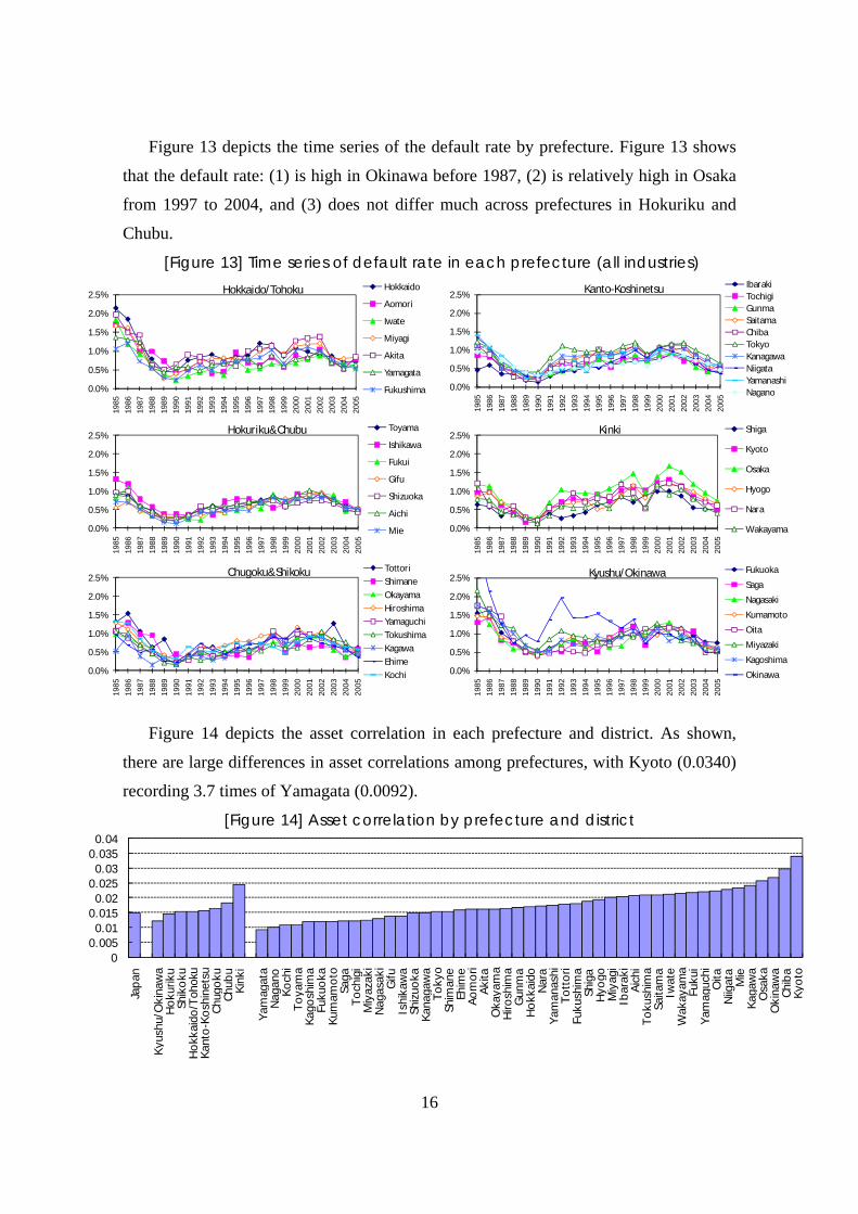
Figure 13 depicts the time series of the default rate by prefecture. Figure 13 shows
that the default rate: (1) is high in Okinawa before 1987, (2) is relatively high in Osaka
from 1997 to 2004, and (3) does not differ much across prefectures in Hokuriku and
Chubu.
[Figure 13] Time series of default rate in each prefecture (all industries)
0.0%
0.5%
1.0%
1.5%
2.0%
2.5%
1985
1986
1987
1988
1989
1990
1991
1992
1993
1994
1995
1996
1997
1998
1999
2000
2001
2002
2003
2004
2005
Hokkaido/Tohoku Hokkaido
Aomori
Iwate
Miyagi
Akita
Yamagata
Fukushima 0.0%
0.5%
1.0%
1.5%
2.0%
2.5%
1985
1986
1987
1988
1989
1990
1991
1992
1993
1994
1995
1996
1997
1998
1999
2000
2001
2002
2003
2004
2005
Kanto-Koshinetsu IbarakiTochigiGunmaSaitamaChibaTokyoKanagawaNiigataYamanashiNagano
0.0%
0.5%
1.0%
1.5%
2.0%
2.5%
1985
1986
1987
1988
1989
1990
1991
1992
1993
1994
1995
1996
1997
1998
1999
2000
2001
2002
2003
2004
2005
Hokuriku&Chubu Toyama
Ishikawa
Fukui
Gifu
Shizuoka
Aichi
Mie 0.0%
0.5%
1.0%
1.5%
2.0%
2.5%
1985
1986
1987
1988
1989
1990
1991
1992
1993
1994
1995
1996
1997
1998
1999
2000
2001
2002
2003
2004
2005
Kinki Shiga
Kyoto
Osaka
Hyogo
Nara
Wakayama
0.0%
0.5%
1.0%
1.5%
2.0%
2.5%
1985
1986
1987
1988
1989
1990
1991
1992
1993
1994
1995
1996
1997
1998
1999
2000
2001
2002
2003
2004
2005
Chugoku&Shikoku TottoriShimaneOkayamaHiroshimaYamaguchiTokushimaKagawaEhimeKochi 0.0%
0.5%
1.0%
1.5%
2.0%
2.5%
1985
1986
1987
1988
1989
1990
1991
1992
1993
1994
1995
1996
1997
1998
1999
2000
2001
2002
2003
2004
2005
Kyushu/Okinawa FukuokaSagaNagasakiKumamotoOitaMiyazakiKagoshimaOkinawa
Figure 14 depicts the asset correlation in each prefecture and district. As shown,
there are large differences in asset correlations among prefectures, with Kyoto (0.0340)
recording 3.7 times of Yamagata (0.0092).
[Figure 14] Asset correlation by prefecture and district
00.0050.01
0.0150.02
0.0250.03
0.0350.04
Japa
n
Kyus
hu/O
kina
wa
Hok
urik
uSh
ikok
uH
okka
ido/
Toho
kuKa
nto-
Kosh
inet
suCh
ugok
uCh
ubu
Kink
i
Yam
a gat
aN
a gan
oKo
chi
Toya
ma
Kago
shim
aFu
kuok
aKu
mam
oto
Saga
Toch
i gi
Miy
azak
iN
agas
aki
Gifu
Ishi
kaw
aSh
izuo
kaKa
naga
wa
Toky
oSh
iman
eEh
ime
Aom
ori
Akita
Oka
yam
aH
irosh
ima
Gun
ma
Hok
kaid
oN
ara
Yam
anas
hiTo
ttor
iFu
kush
ima
Shig
aH
yogo
Miy
agi
Ibar
aki
Aich
iTo
kush
ima
Saita
ma
Iwat
eW
akay
ama
Fuku
iYa
ma g
uchi
Oita
Niig
ata
Mie
Kaga
wa
Osa
kaO
kina
wa
Chib
aK y
oto
17
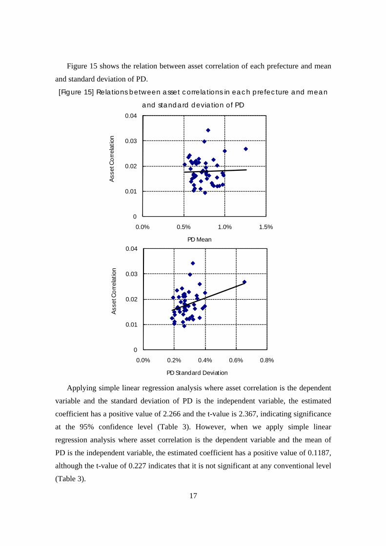
Figure 15 shows the relation between asset correlation of each prefecture and mean
and standard deviation of PD.
[Figure 15] Relations between asset correlations in each prefecture and mean
and standard deviation of PD
Applying simple linear regression analysis where asset correlation is the dependent
variable and the standard deviation of PD is the independent variable, the estimated
coefficient has a positive value of 2.266 and the t-value is 2.367, indicating significance
at the 95% confidence level (Table 3). However, when we apply simple linear
regression analysis where asset correlation is the dependent variable and the mean of
PD is the independent variable, the estimated coefficient has a positive value of 0.1187,
although the t-value of 0.227 indicates that it is not significant at any conventional level
(Table 3).
0
0.01
0.02
0.03
0.04
0.0% 0.5% 1.0% 1.5%
Ass
et C
orr
elat
ion
PD Mean
0
0.01
0.02
0.03
0.04
0.0% 0.2% 0.4% 0.6% 0.8%
Ass
et C
orr
elat
ion
PD Standard Deviation
18
[Table 3] Result of simple linear regression analysis
(the dependent variable is asset correlation)21 Independent
variable Estimated coefficient
(t-value) Intercept (t-value)
Coefficient of determination
PD mean 0.1187 (0.227)
0.01687 (4.234***)
0.00114
PD standard deviation
2.266 (2.367**)
0.01132 (4.017***)
0.1107
In conclusion, these results demonstrate that the relation between asset correlation
and the standard deviation of the PD is positive. For example, the asset correlation in
Okinawa, which has the largest standard deviation of the PD, is the third highest across
all prefectures.
4. Conclusion
This paper analyzed the asset correlations of active and default Japanese companies.
The data of these companies were grouped by industry type, company size, credit rating
and region. The conclusions from this paper are as follows.
(1) The Multi Index Model was used because it was necessary to analyze at least both
the first and the second components of the changes in default rate in order to explain
changes in the default rate. Using principal component analysis, we cannot explain
the cumulative R-squared of industry type, company size and region using only the
first component, but can explain 90% of the R-squared using both the first and the
second components.
(2) Asset correlations differ by industry, company size, credit rating and region. This
means that it is not appropriate to use a common asset correlation in the credit
portfolio.
(3) When the data are grouped by company size, asset correlation is high in large
companies and low in small companies. Our hypothesis is that changes in the
performance of large companies are similar to changes in the entire economic
system, meaning, for example, a boom for all companies or higher performance in
21 *** and ** indicate significance at the 99% and 95% confidence level, respectively.
19
the industry or region to which the company belongs. Therefore, the common factor
easily affects the performance of large companies and so the asset correlation of
these companies is high. On the other hand, the situation of the individual company
rather than the economic system affects the performance of small companies.
Therefore, asset correlations for small companies and personal companies are lower.
(4) Asset correlation is high in companies with high and low credit ratings and low in
companies with middle credit ratings. In other words, the shapes of asset correlation
functions are convex downward in credit ratings.
(5) The asset correlation among prefectures makes a great difference, with the
maximum difference being 3.7 times. In addition, asset correlation and the standard
deviation of the PD are positively related, and a prefecture where the volatility of
the default rate is large tends to have a large asset correlation.
This analysis highlights the fact that asset correlation is an important subject for
credit portfolio analysis in financial institutions. We expect that the findings of this
paper will enable financial institutions in Japan to improve their credit risk management.
20
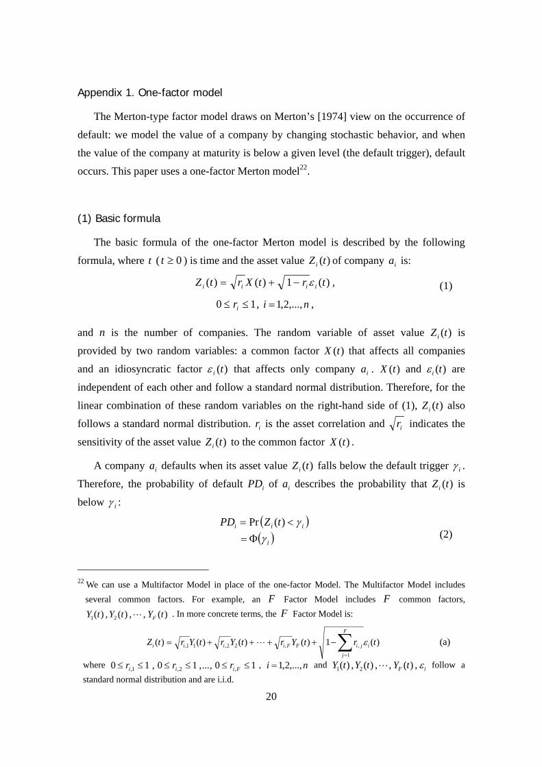
Appendix 1. One-factor model
The Merton-type factor model draws on Merton’s [1974] view on the occurrence of
default: we model the value of a company by changing stochastic behavior, and when
the value of the company at maturity is below a given level (the default trigger), default
occurs. This paper uses a one-factor Merton model22.
(1) Basic formula
The basic formula of the one-factor Merton model is described by the following
formula, where t ( 0≥t ) is time and the asset value )(tZi of company ia is:
)(1)()( trtXrtZ iiii ε−+= , (1)
10 ≤≤ ir , ni ,...,2,1= ,
and n is the number of companies. The random variable of asset value )(tZi is
provided by two random variables: a common factor )(tX that affects all companies
and an idiosyncratic factor )(tiε that affects only company ia . )(tX and )(tiε are
independent of each other and follow a standard normal distribution. Therefore, for the
linear combination of these random variables on the right-hand side of (1), )(tZi also
follows a standard normal distribution. ir is the asset correlation and ir indicates the
sensitivity of the asset value )(tZi to the common factor )(tX .
A company ia defaults when its asset value )(tZi falls below the default trigger iγ .
Therefore, the probability of default iPD of ia describes the probability that )(tZi is
below iγ :
( )( )i
iii tZPDγ
γΦ=
<= )(Pr (2)
22 We can use a Multifactor Model in place of the one-factor Model. The Multifactor Model includes
several common factors. For example, an F Factor Model includes F common factors,
)(,,)(,)( 21 tYtYtY FL . In more concrete terms, the F Factor Model is:
)(1)()()()(1
,,22,11, trtYrtYrtYrtZ i
F
j
jiFFiiii ε∑=
−++++= L (a)
where 10,...,10,10 ,2,1, ≤≤≤≤≤≤ Fiii rrr , ni ,...,2,1= and iF tYtYtY ε,)(,,)(,)( 21 L follow a standard normal distribution and are i.i.d.
21
∫ ∞−
−=Φx
duux )2/exp(21)( 2
π
(2) Single Index Model
The Single Index Model is a type of one-factor Merton model. The Single Index
Model imposes a single asset correlation for each group of companies decided by
certain criteria, whereas the basic formula (1) imposes different asset correlations ir for
each company ia .
In a set A composed of companies ),,1( niai L= , the companies are grouped
under certain criteria and the groups are described by },,{ )()(1
)( lm
lll
SSS LL= . lm shows
the number of groups. Each )(lS is composed of a subset ),,1()(l
lk mkS L= , the element
of which is the company ia . l is the criterion used for making the group and k is the
kind of group. For example, when l is “industry type”, k is “manufacturing”,
“construction”, and so on.
In any l , )(lS satisfies:
},,{,,, )()(1
)()()(
1
)( lm
lllj
li
m
k
lk l
l
SSSjiSSSA LLU =≠=∩==
φ .
To simplify the formula, we set only one l in )(lS (in other words, we decide the
grouping criterion) and describe },,{ 1 mSSS L= instead of )(lS in the following parts.
We set the default trigger kC and asset correlations kρ , ( kji rr ρ== , kji Saa ∈, ,
ji ≠ ) of the company that belongs to the same group kS as the same23. In other words,
when ki Sa ∈ , we can rewrite (1) and (2) as (3) and (4), respectively:
)(1)()( ttXtZ ikki ερρ −+= (3)
( )( )k
kii
CCtZPD
Φ=<= )(Pr
(4)
We set these hypotheses because many credit risk managers set parameters not for
23 We hypothesize that asset correlation kρ and default trigger kC are the same in the same group. If we
need to set several default triggers in the same group, we also need to set different triggers for different groups. This paper, like many others, hypothesizes that each group has the same default trigger kC (see Appendix 2).
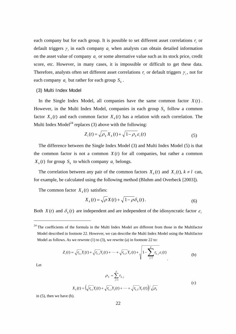
22
each company but for each group. It is possible to set different asset correlations ir or
default triggers iγ in each company ia when analysts can obtain detailed information
on the asset value of company ia or some alternative value such as its stock price, credit
score, etc. However, in many cases, it is impossible or difficult to get these data.
Therefore, analysts often set different asset correlations ir or default triggers iγ , not for
each company ia but rather for each group kS .
(3) Multi Index Model
In the Single Index Model, all companies have the same common factor )(tX .
However, in the Multi Index Model, companies in each group kS follow a common
factor )(tX k and each common factor )(tX k has a relation with each correlation. The
Multi Index Model24 replaces (3) above with the following:
)(1)()( ttXtZ ikkki ερρ −+= (5)
The difference between the Single Index Model (3) and Multi Index Model (5) is that
the common factor is not a common )(tX for all companies, but rather a common
)(tX k for group kS to which company ia belongs.
The correlation between any pair of the common factors )(tX k and lktX l ≠),( can,
for example, be calculated using the following method (Bluhm and Overbeck [2003]).
The common factor )(tX k satisfies:
)(1)()( ttXtX kk δρρ −+= . (6)
Both )(tX and )(tkδ are independent and are independent of the idiosyncratic factor iε
24 The coefficients of the formula in the Multi Index Model are different from those in the Multifactor
Model described in footnote 22. However, we can describe the Multi Index Model using the Multifactor Model as follows. As we rewrote (1) to (3), we rewrite (a) in footnote 22 to:
)(1)()()()(1
,,22,11, trtYrtYrtYrtZ i
F
j
jkFFkkki ε∑=
−++++= L
.
(b)
Let
∑=
=F
jjkk r
1,ρ
( ) kFFkkkk tYrtYrtYrtX ρ)()()()( ,22,11, +++= L (c)
in (5), then we have (b).
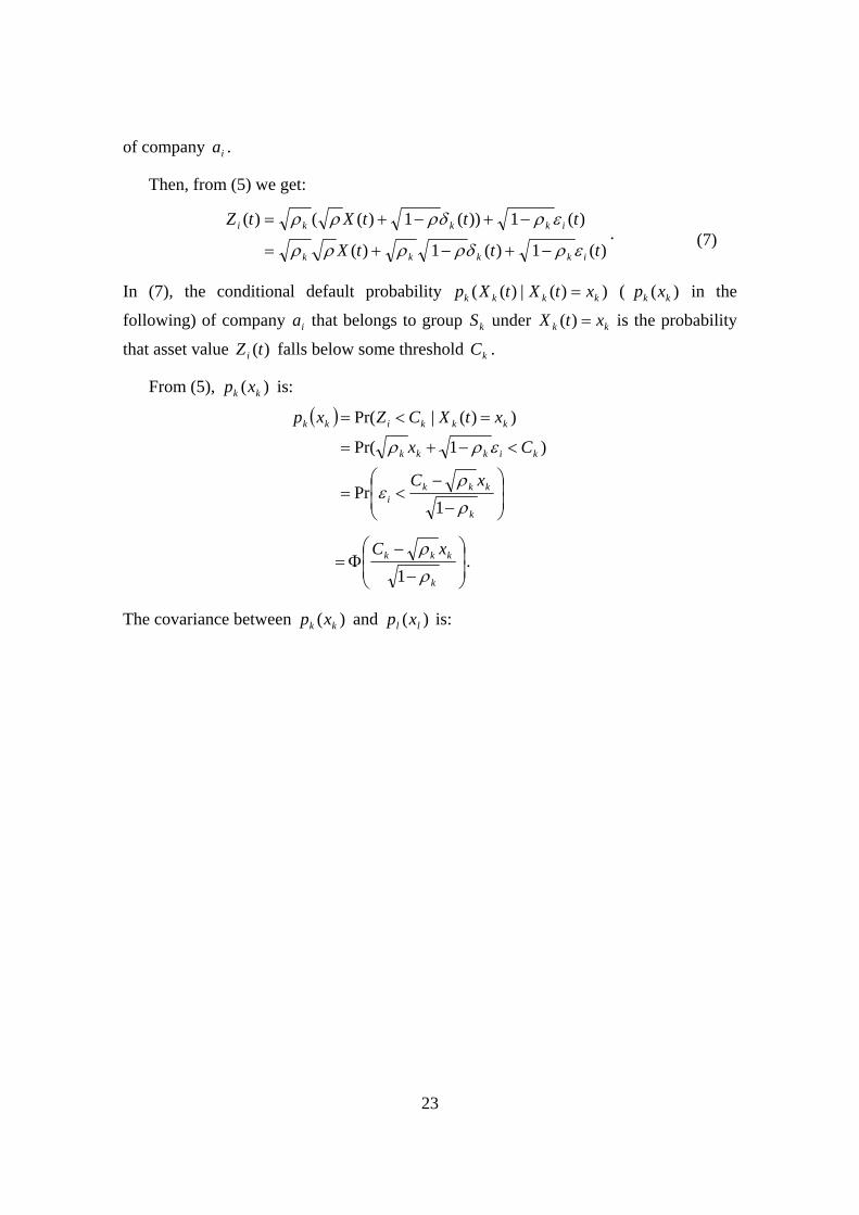
23
of company ia .
Then, from (5) we get:
)(1)(1)(
)(1))(1)(()(
tttX
tttXtZ
ikkkk
ikkki
ερδρρρρ
ερδρρρ
−+−+=
−+−+=. (7)
In (7), the conditional default probability ))(|)(( kkkk xtXtXp = ( )( kk xp in the
following) of company ia that belongs to group kS under kk xtX =)( is the probability
that asset value )(tZi falls below some threshold kC .
From (5), )( kk xp is:
( )
⎟⎟⎠
⎞⎜⎜⎝
⎛
−
−<=
<−+=
=<=
k
kkki
kikkk
kkkikk
xC
Cx
xtXCZxp
ρρ
ε
ερρ
1Pr
)1Pr(
))(|Pr(
⎟⎟⎠
⎞⎜⎜⎝
⎛
−
−Φ=
k
kkk xCρρ
1.
The covariance between )( kk xp and )( ll xp is:
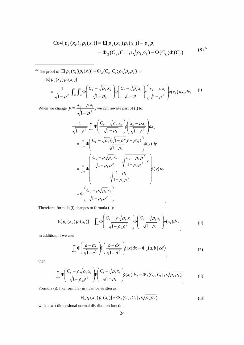
24
)()()|,(
)]()([E)](),([Cov
2 lklklk
lkllkkllkk
CCCC
ppxpxpxpxp
ΦΦ−Φ=
−=
ρρρ, (8)25
25 The proof of );,()]()([E 2 lklkllkk CCxpxp ρρρΦ= is
lkllk
l
lll
k
kkk
llkk
dxdxxxxxCxC
xpxp
)(1111
1
)]()([E
22φ
ρ
ρφ
ρ
ρ
ρ
ρ
ρ ⎟⎟
⎠
⎞
⎜⎜
⎝
⎛
−
−⎟⎟⎠
⎞⎜⎜⎝
⎛
−
−Φ⎟⎟⎠
⎞⎜⎜⎝
⎛
−
−Φ
−= ∫ ∫
∞
∞−
∞
∞−
.
(i)
When we change 21 ρ
ρ
−
−≡ lk xx
y , we can rewrite part of (i) to:
⎟⎟
⎠
⎞
⎜⎜
⎝
⎛
−
−Φ=
⎟⎟⎟⎟⎟⎟
⎠
⎞
⎜⎜⎜⎜⎜⎜
⎝
⎛
−−
−−
−−
−
Φ=
⎟⎟
⎠
⎞
⎜⎜
⎝
⎛
−
+−−Φ=
⎟⎟
⎠
⎞
⎜⎜
⎝
⎛
−
−⎟⎟⎠
⎞⎜⎜⎝
⎛
−
−Φ
−
∫
∫
∫
∞
∞−
∞
∞−
∞
∞−
2
2
2
2
2
2
22
1
)(
11
11
)(1
)1(
111
1
ρρ
ρρ
φ
ρρρ
ρρρρρ
ρρ
ρρ
φρ
ρρρ
ρ
ρφ
ρ
ρ
ρ
k
lkk
k
k
k
kk
k
lkk
k
lkk
klk
k
kkk
xC
dyy
yxC
dyyxyC
dxxxxC
.
Therefore, formula (i) changes to formula (ii):
ll
l
lll
k
lkkllkk dxx
xCxCxpxp )(
11)]()([E
2φ
ρ
ρ
ρρ
ρρ⎟⎟⎠
⎞⎜⎜⎝
⎛
−
−Φ⎟⎟
⎠
⎞
⎜⎜
⎝
⎛
−
−Φ= ∫
∞
∞−
.
(ii)
In addition, if we use:
( )cdbadxxd
dxb
c
cxa |,)(11
222Φ=⎟
⎟⎠
⎞⎜⎜⎝
⎛
−
−Φ⎟⎟⎠
⎞⎜⎜⎝
⎛
−
−Φ∫
∞
∞−φ
, (*)
then
)|,()(11
22 lklklll
lll
k
lkk CCdxxxCxC
ρρρφρ
ρ
ρρ
ρρΦ=⎟
⎟⎠
⎞⎜⎜⎝
⎛
−
−Φ⎟⎟
⎠
⎞
⎜⎜
⎝
⎛
−
−Φ∫
∞
∞−
.
(ii)’
Formula (i), like formula (iii), can be written as:
)|,()]()([E 2 lklkllkk CCxpxp ρρρΦ= (iii)
with a two-dimensional normal distribution function.
25
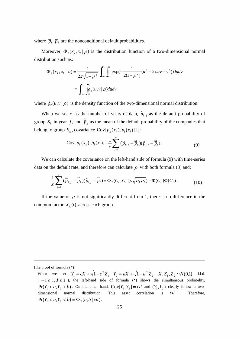
where lk pp , are the nonconditional default probabilities.
Moreover, )|,(2 ρlk xxΦ is the distribution function of a two-dimensional normal
distribution such as:
dudvvuvuxxk lx x
lk ∫ ∫∞− ∞−
+−−
−−
=Φ ))2()1(2
1exp(12
1)|,( 22222 ρ
ρρπρ
dudvvuk lx x
∫ ∫∞− ∞−
≡ )|,(2 ρφ ,
where )|,(2 ρφ vu is the density function of the two-dimensional normal distribution.
When we set κ as the number of years of data, jkp ,~ as the default probability of
group kS in year j , and kp~ as the mean of the default probability of the companies that
belong to group kS , covariance )](),([Cov llkk xpxp is:
)](),([Cov llkk xpxp = ∑=
−−κ
κ1
,, )~~)(~~(1
j
ljlkjk pppp . (9)
We can calculate the covariance on the left-hand side of formula (9) with time-series
data on the default rate, and therefore can calculate ρ with both formula (8) and:
)()()|,()~~)(~~(12
1
,, lklklk
j
ljlkjk CCCCpppp ΦΦ−Φ=−−∑=
ρρρκ
κ
. (10)
If the value of ρ is not significantly different from 1, there is no difference in the
common factor )(tX k across each group.
[the proof of formula (*)]
When we set 12
1 1 ZccXY −+= 22
2 1 ZddXY −+= )1,0(,, 21 NZZX ~ i.i.d. ( 1,1 ≤≤− dc ), the left-hand side of formula (*) shows the simultaneous probability,
),Pr( 21 bYaY << . On the other hand, cdYY =],[Cov 21 and ),( 21 YY clearly follow a two-dimensional normal distribution. This asset correlation is cd . Therefore,
)|,(),Pr( 221 cdbabYaY Φ=<< .
26
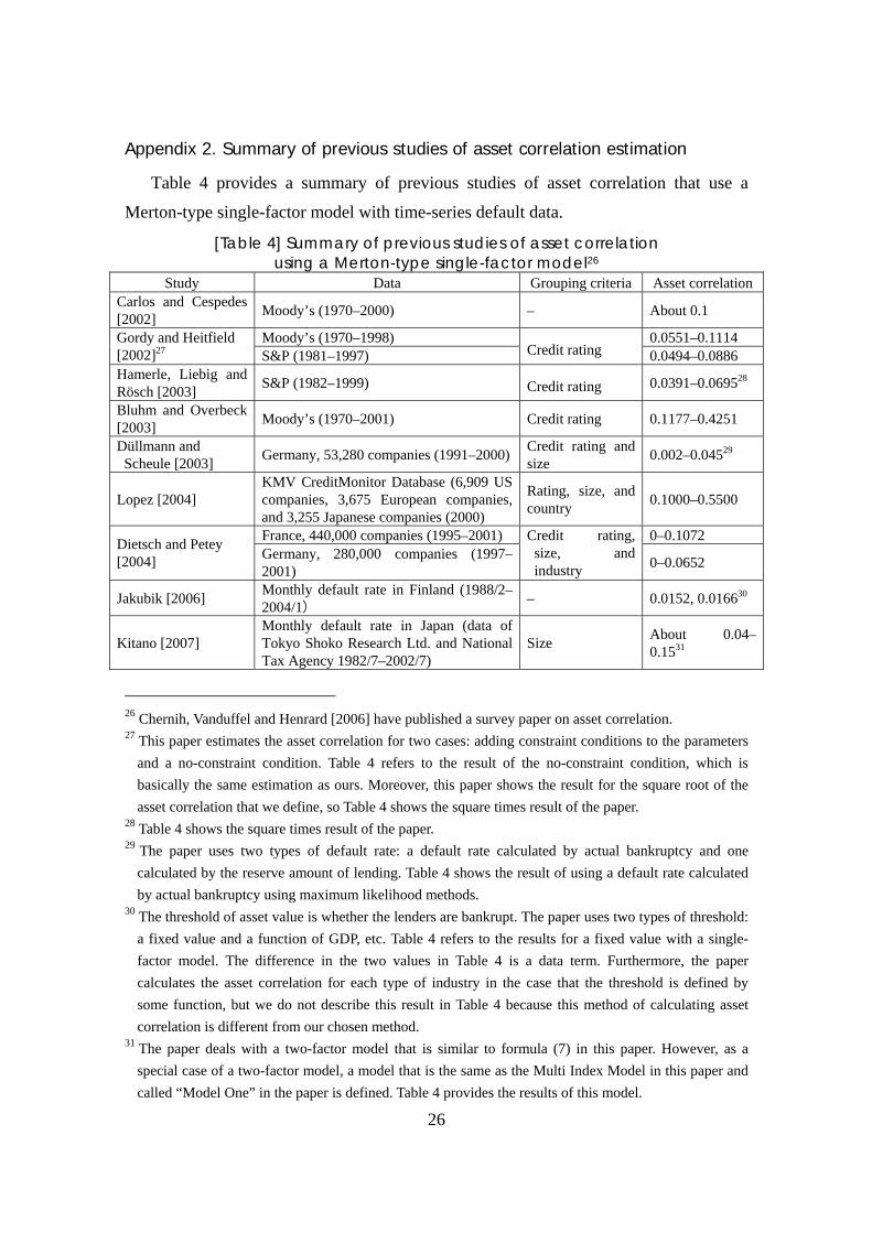
Appendix 2. Summary of previous studies of asset correlation estimation
Table 4 provides a summary of previous studies of asset correlation that use a
Merton-type single-factor model with time-series default data.
[Table 4] Summary of previous studies of asset correlation using a Merton-type single-factor model26
Study Data Grouping criteria Asset correlationCarlos and Cespedes [2002] Moody’s (1970–2000) – About 0.1
Moody’s (1970–1998) 0.0551–0.1114 Gordy and Heitfield [2002]27 S&P (1981–1997) Credit rating 0.0494–0.0886 Hamerle, Liebig and Rösch [2003] S&P (1982–1999) Credit rating 0.0391–0.069528
Bluhm and Overbeck [2003] Moody’s (1970–2001) Credit rating 0.1177–0.4251
Düllmann and Scheule [2003] Germany, 53,280 companies (1991–2000) Credit rating and
size 0.002–0.04529
Lopez [2004] KMV CreditMonitor Database (6,909 US companies, 3,675 European companies, and 3,255 Japanese companies (2000)
Rating, size, and country 0.1000–0.5500
France, 440,000 companies (1995–2001) 0–0.1072 Dietsch and Petey [2004] Germany, 280,000 companies (1997–
2001)
Credit rating, size, and industry 0–0.0652
Jakubik [2006] Monthly default rate in Finland (1988/2–2004/1) – 0.0152, 0.016630
Kitano [2007] Monthly default rate in Japan (data of Tokyo Shoko Research Ltd. and National Tax Agency 1982/7–2002/7)
Size About 0.04–0.1531
26 Chernih, Vanduffel and Henrard [2006] have published a survey paper on asset correlation. 27 This paper estimates the asset correlation for two cases: adding constraint conditions to the parameters
and a no-constraint condition. Table 4 refers to the result of the no-constraint condition, which is basically the same estimation as ours. Moreover, this paper shows the result for the square root of the asset correlation that we define, so Table 4 shows the square times result of the paper.
28 Table 4 shows the square times result of the paper. 29 The paper uses two types of default rate: a default rate calculated by actual bankruptcy and one
calculated by the reserve amount of lending. Table 4 shows the result of using a default rate calculated by actual bankruptcy using maximum likelihood methods.
30 The threshold of asset value is whether the lenders are bankrupt. The paper uses two types of threshold: a fixed value and a function of GDP, etc. Table 4 refers to the results for a fixed value with a single-factor model. The difference in the two values in Table 4 is a data term. Furthermore, the paper calculates the asset correlation for each type of industry in the case that the threshold is defined by some function, but we do not describe this result in Table 4 because this method of calculating asset correlation is different from our chosen method.
31 The paper deals with a two-factor model that is similar to formula (7) in this paper. However, as a special case of a two-factor model, a model that is the same as the Multi Index Model in this paper and called “Model One” in the paper is defined. Table 4 provides the results of this model.
27
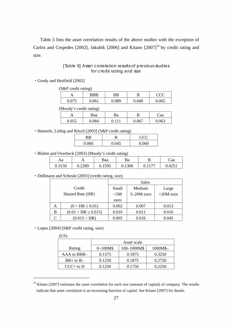
Table 5 lists the asset correlation results of the above studies with the exception of
Carlos and Cespedes [2002], Jakubik [2006] and Kitano [2007]32 by credit rating and
size.
[Table 5] Asset correlation results of previous studies for credit rating and size
・Gordy and Heitfield [2002]
(S&P credit rating) A BBB BB B CCC
0.075 0.061 0.089 0.049 0.065
(Moody’s credit rating) A Baa Ba B Caa
0.055 0.084 0.111 0.067 0.063
・Hamerle, Liebig and Rösch [2003] (S&P credit rating) BB B CCC
0.060 0.045 0.069
・Bluhm and Overbeck [2003] (Moody’s credit rating) Aa A Baa Ba B Caa
0.3150 0.2289 0.1595 0.1300 0.1177 0.4251
・Düllmann and Scheule [2003] (credit rating, size) Sales
Credit Hazard Rate (HR)
Small <5M euro
Medium 5–20M euro
Large >20M euro
A (0 < HR ≤ 0.01) 0.002 0.007 0.013 B (0.01 < HR ≤ 0.015) 0.010 0.011 0.016 C (0.015 < HR) 0.005 0.016 0.045
・Lopez [2004] (S&P credit rating, size)
(US) Asset scale
Rating 0–100M$ 100–1000M$ 1000M$– AAA to BBB– 0.1375 0.1875 0.3250
BB+ to B– 0.1250 0.1875 0.2750 CCC+ to D 0.1250 0.1750 0.2250
32 Kitano [2007] estimates the asset correlation for each size (amount of capital) of company. The results
indicate that asset correlation is an increasing function of capital. See Kitano [2007] for details.
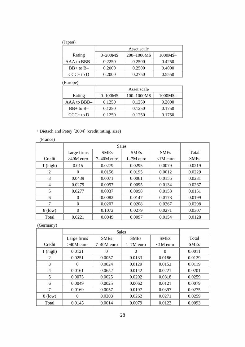
28
(Japan) Asset scale
Rating 0–200M$ 200–1000M$ 1000M$– AAA to BBB– 0.2250 0.2500 0.4250
BB+ to B– 0.2000 0.2500 0.4000 CCC+ to D 0.2000 0.2750 0.5550
(Europe) Asset scale
Rating 0–100M$ 100–1000M$ 1000M$– AAA to BBB– 0.1250 0.1250 0.2000
BB+ to B– 0.1250 0.1250 0.1750 CCC+ to D 0.1250 0.1250 0.1750
・Dietsch and Petey [2004] (credit rating, size)
(France) Sales
Credit
Large firms >40M euro
SMEs 7–40M euro
SMEs 1–7M euro
SMEs <1M euro
Total SMEs
1 (high) 0.015 0.0279 0.0295 0.0079 0.0219 2 0 0.0156 0.0195 0.0012 0.0229 3 0.0439 0.0071 0.0061 0.0155 0.0231 4 0.0279 0.0057 0.0095 0.0134 0.0267 5 0.0277 0.0037 0.0098 0.0153 0.0151 6 0 0.0082 0.0147 0.0178 0.0199 7 0 0.0207 0.0208 0.0267 0.0298
8 (low) 0 0.1072 0.0279 0.0271 0.0307 Total 0.0221 0.0049 0.0097 0.0154 0.0128
(Germany) Sales
Credit
Large firms >40M euro
SMEs 7–40M euro
SMEs 1–7M euro
SMEs <1M euro
Total SMEs
1 (high) 0.0121 0 0 0 0.0011 2 0.0251 0.0057 0.0133 0.0186 0.0129 3 0 0.0024 0.0129 0.0152 0.0119 4 0.0161 0.0652 0.0142 0.0221 0.0201 5 0.0075 0.0025 0.0202 0.0318 0.0259 6 0.0049 0.0025 0.0062 0.0121 0.0079 7 0.0169 0.0057 0.0197 0.0397 0.0275
8 (low) 0 0.0203 0.0262 0.0271 0.0259 Total 0.0145 0.0014 0.0079 0.0123 0.0093
29
Appendix 3. Estimation methods and differences in results
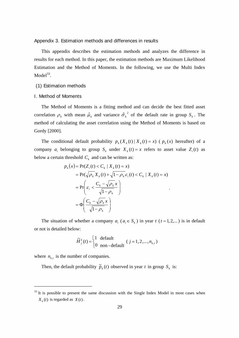
This appendix describes the estimation methods and analyzes the difference in
results for each method. In this paper, the estimation methods are Maximum Likelihood
Estimation and the Method of Moments. In the following, we use the Multi Index
Model33.
(1) Estimation methods
I. Method of Moments
The Method of Moments is a fitting method and can decide the best fitted asset
correlation kρ with mean kµ̂ and variance 2ˆ kσ of the default rate in group kS . The
method of calculating the asset correlation using the Method of Moments is based on
Gordy [2000].
The conditional default probability ))(|)(( xtXtXp kkk = ( )(xpk hereafter) of a
company ia belonging to group kS under xtX k =)( refers to asset value )(tZi as
below a certain threshold kC and can be written as:
( )
⎟⎟⎠
⎞⎜⎜⎝
⎛
−
−Φ=
⎟⎟⎠
⎞⎜⎜⎝
⎛
−
−<=
=<−+=
=<=
k
kk
k
kki
kkikkk
kkik
xC
xC
xtXCttX
xtXCtZxp
ρ
ρ
ρ
ρε
ερρ
1
1Pr
))(|)(1)(Pr(
))(|)(Pr(
.
The situation of whether a company ia ( ki Sa ∈ ) in year t ( ,...2,1=t ) is in default
or not is detailed below:
⎩⎨⎧
=01
)(~ tH kj
default-nondefault
( tknj ,,...,2,1= )
where tkn , is the number of companies.
Then, the default probability )(~ tpk observed in year t in group kS is:
33 It is possible to present the same discussion with the Single Index Model in most cases when
)(tX k is regarded as )(tX .
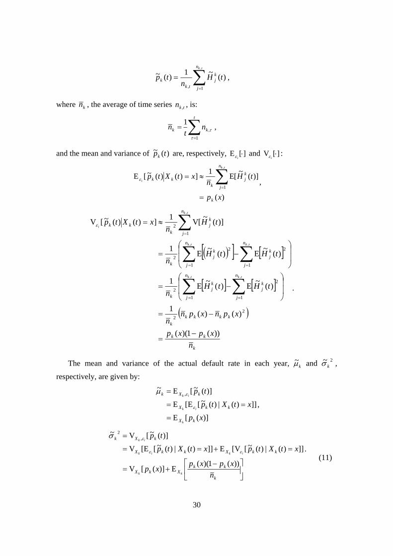
30
∑=
=tkn
j
kj
tkk tH
ntp
,
1,
)(~1)(~ ,
where kn , the average of time series tkn , , is:
∑=
=t
kk nt
n1
,1
τ
τ ,
and the mean and variance of )(~ tpk are, respectively, ][E ⋅iε
and ][V ⋅iε
:
)(
)](~[E1])()(~[E,
1
xp
tHn
xtXtp
k
n
j
kj
kkk
tk
i
=
≈= ∑=
ε ,
( )[ ] [ ]
[ ] [ ]
( )
k
kk
kkkkk
n
j
kj
n
j
kj
k
n
j
kj
n
j
kj
k
n
j
kj
kkk
nxpxp
xpnxpnn
tHtHn
tHtHn
tHn
xtXtp
tktk
tktk
tk
i
))(1)((
)()(1
)(~E)(~E1
)(~E)(~E1
)](~[V1])()(~[V
22
1
2
12
1
2
1
2
2
12
,,
,,
,
−=
−=
⎟⎟
⎠
⎞
⎜⎜
⎝
⎛−=
⎟⎟
⎠
⎞
⎜⎜
⎝
⎛−=
≈=
∑∑
∑∑
∑
==
==
=
ε
.
The mean and variance of the actual default rate in each year, kµ~ and 2~kσ ,
respectively, are given by:
)]([E
]])(|)(~[E[E
)](~[E~,
xp
xtXtp
tp
kX
kkX
kXk
k
ik
ik
=
==
=
ε
εµ
,
⎥⎦
⎤⎢⎣
⎡ −+=
=+==
=
k
kkXkX
kkXkkX
kXk
nxpxp
xp
xtXtpxtXtp
tp
kk
ikik
ik
))(1)((E)]([V
]])(|)(~[V[E]])(|)(~[[EV
)](~[V~,
2
εε
εσ
. (11)
31
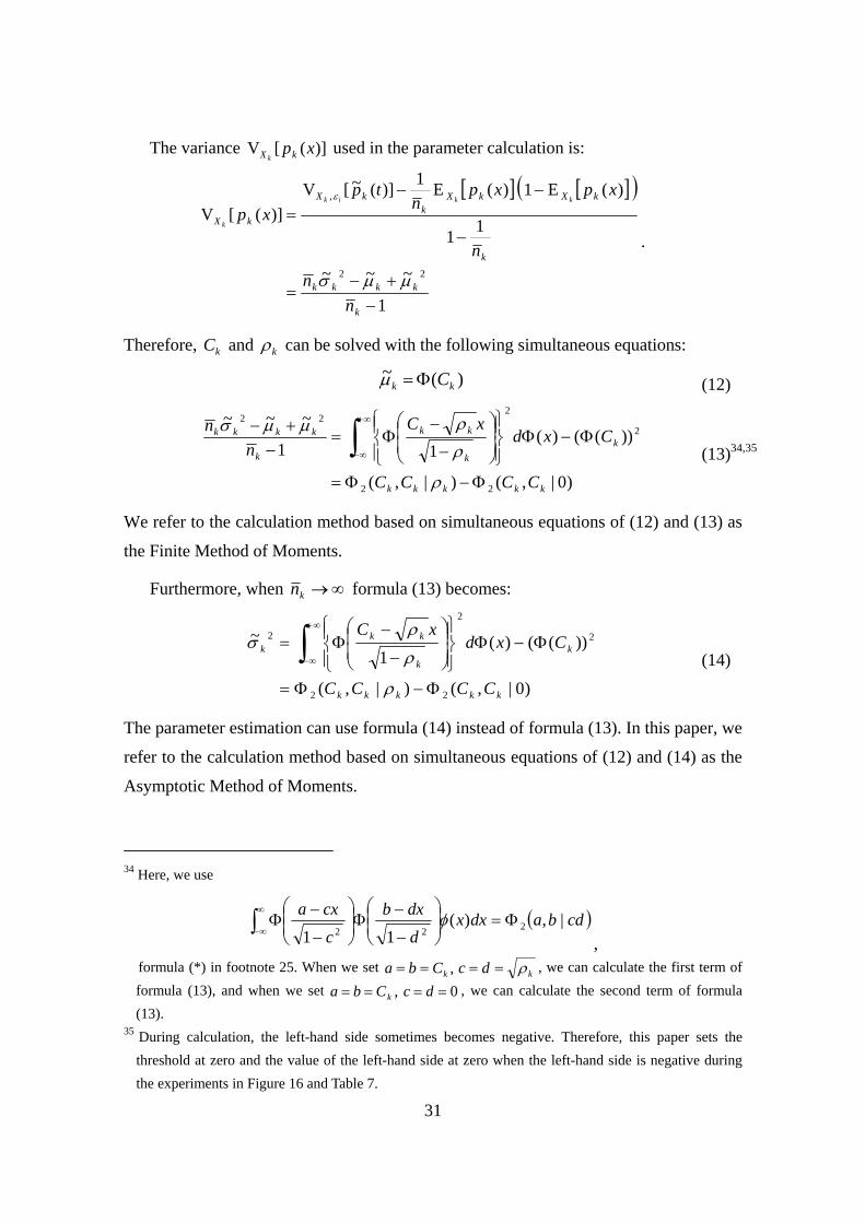
The variance )]([V xpkX k used in the parameter calculation is:
[ ] [ ]( )
1
~~~
11
)(E1)(E1)](~[V)]([V
22
,
−+−
=
−
−−=
k
kkkk
k
kXkXk
kX
kX
nn
n
xpxpn
tpxp
kkik
k
µµσ
ε
.
Therefore, kC and kρ can be solved with the following simultaneous equations:
)(~kk CΦ=µ (12)
)0|,()|,(
))(()(11
~~~
22
2
222
kkkkk
kk
kk
k
kkkk
CCCC
CxdxC
nn
Φ−Φ=
Φ−Φ⎪⎭
⎪⎬⎫
⎪⎩
⎪⎨⎧
⎟⎟⎠
⎞⎜⎜⎝
⎛
−
−Φ=
−+− ∫
∞+
∞−
ρ
ρρµµσ
(13)34,35
We refer to the calculation method based on simultaneous equations of (12) and (13) as
the Finite Method of Moments.
Furthermore, when ∞→kn formula (13) becomes:
)0|,()|,(
))(()(1
~
22
2
2
2
kkkkk
kk
kkk
CCCC
CxdxC
Φ−Φ=
Φ−Φ⎪⎭
⎪⎬⎫
⎪⎩
⎪⎨⎧
⎟⎟⎠
⎞⎜⎜⎝
⎛
−
−Φ= ∫
∞+
∞−
ρ
ρ
ρσ (14)
The parameter estimation can use formula (14) instead of formula (13). In this paper, we
refer to the calculation method based on simultaneous equations of (12) and (14) as the
Asymptotic Method of Moments.
34 Here, we use
( )cdbadxxd
dxb
c
cxa |,)(11
222Φ=⎟
⎟⎠
⎞⎜⎜⎝
⎛
−
−Φ⎟⎟⎠
⎞⎜⎜⎝
⎛
−
−Φ∫
∞
∞−φ
,
formula (*) in footnote 25. When we set kk dcCba ρ==== , , we can calculate the first term of formula (13), and when we set 0, ==== dcCba k , we can calculate the second term of formula (13).
35 During calculation, the left-hand side sometimes becomes negative. Therefore, this paper sets the threshold at zero and the value of the left-hand side at zero when the left-hand side is negative during the experiments in Figure 16 and Table 7.
32
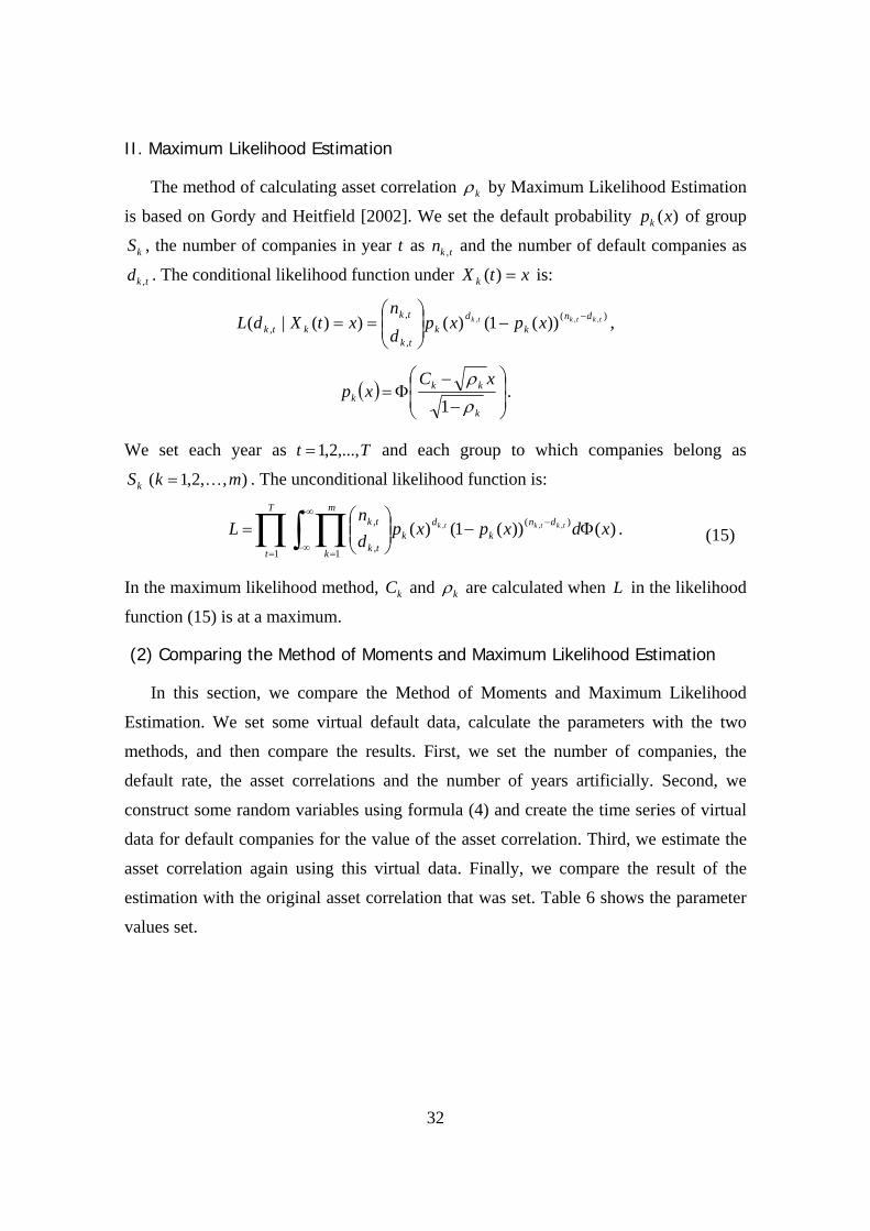
II. Maximum Likelihood Estimation
The method of calculating asset correlation kρ by Maximum Likelihood Estimation
is based on Gordy and Heitfield [2002]. We set the default probability )(xpk of group
kS , the number of companies in year t as tkn , and the number of default companies as
tkd , . The conditional likelihood function under xtX k =)( is:
)(
,
,,
,,, ))(1()())(|( tktktk dnk
dk
tk
tkktk xpxp
dn
xtXdL −−⎟⎟⎠
⎞⎜⎜⎝
⎛== ,
( ) ⎟⎟⎠
⎞⎜⎜⎝
⎛
−
−Φ=
k
kkk
xCxp
ρρ
1.
We set each year as Tt ,...,2,1= and each group to which companies belong as
kS ),,2,1( mk K= . The unconditional likelihood function is:
)())(1()(1 1
)(
,
, ,,,∏∫ ∏=
+∞
∞−=
− Φ−⎟⎟⎠
⎞⎜⎜⎝
⎛=
T
t
m
k
dnk
dk
tk
tk xdxpxpdn
L tktktk . (15)
In the maximum likelihood method, kC and kρ are calculated when L in the likelihood
function (15) is at a maximum.
(2) Comparing the Method of Moments and Maximum Likelihood Estimation
In this section, we compare the Method of Moments and Maximum Likelihood
Estimation. We set some virtual default data, calculate the parameters with the two
methods, and then compare the results. First, we set the number of companies, the
default rate, the asset correlations and the number of years artificially. Second, we
construct some random variables using formula (4) and create the time series of virtual
data for default companies for the value of the asset correlation. Third, we estimate the
asset correlation again using this virtual data. Finally, we compare the result of the
estimation with the original asset correlation that was set. Table 6 shows the parameter
values set.
33
[Table 6] Parameter settings
Number of companies 32(≒ 101.5) – 100,000(= 105), each 100.25
Default rate 1%
Asset correlation 0.01, 0.10, 0.20
Number of years 10 (independent of one another)
Number of experiments 10,000
Using the parameters in Table 6, we create virtual data on the number of default and
active companies using Monte Carlo methods and estimate the asset correlations for 10
years. This process recurs 10,000 times and we calculate the average, 99% point, 90%
point, 10% point and 1% point. Figure 16 shows the results36.
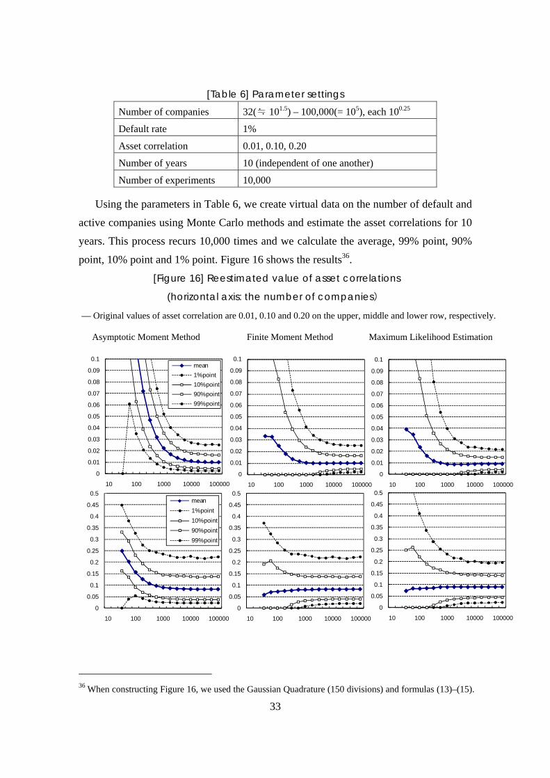
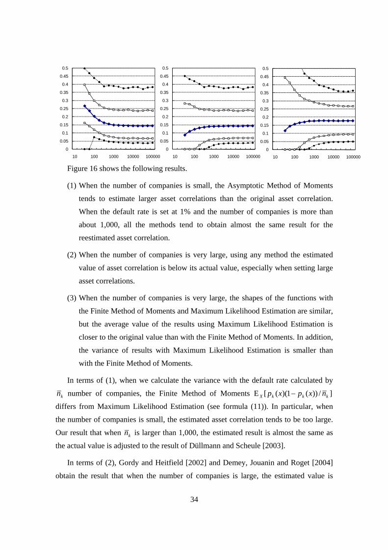
[Figure 16] Reestimated value of asset correlations
(horizontal axis: the number of companies)
— Original values of asset correlation are 0.01, 0.10 and 0.20 on the upper, middle and lower row, respectively.
36 When constructing Figure 16, we used the Gaussian Quadrature (150 divisions) and formulas (13)–(15).
Asymptotic Moment Method Finite Moment Method Maximum Likelihood Estimation
0
0.05
0.1
0.15
0.2
0.25
0.3
0.35
0.4
0.45
0.5
10 100 1000 10000 100000
mean1% point10% point90% point99% point
0
0.05
0.1
0.15
0.2
0.25
0.3
0.35
0.4
0.45
0.5
10 100 1000 10000 100000
0
0.05
0.1
0.15
0.2
0.25
0.3
0.35
0.4
0.45
0.5
10 100 1000 10000 100000
0
0.01
0.02
0.03
0.04
0.05
0.06
0.07
0.08
0.09
0.1
10 100 1000 10000 100000
mean1% point10% point90% point99% point
0
0.01
0.02
0.03
0.04
0.05
0.06
0.07
0.08
0.09
0.1
10 100 1000 10000 100000
0
0.01
0.02
0.03
0.04
0.05
0.06
0.07
0.08
0.09
0.1
10 100 1000 10000 100000
34
Figure 16 shows the following results.
(1) When the number of companies is small, the Asymptotic Method of Moments
tends to estimate larger asset correlations than the original asset correlation.
When the default rate is set at 1% and the number of companies is more than
about 1,000, all the methods tend to obtain almost the same result for the
reestimated asset correlation.
(2) When the number of companies is very large, using any method the estimated
value of asset correlation is below its actual value, especially when setting large
asset correlations.
(3) When the number of companies is very large, the shapes of the functions with
the Finite Method of Moments and Maximum Likelihood Estimation are similar,
but the average value of the results using Maximum Likelihood Estimation is
closer to the original value than with the Finite Method of Moments. In addition,
the variance of results with Maximum Likelihood Estimation is smaller than
with the Finite Method of Moments.
In terms of (1), when we calculate the variance with the default rate calculated by
kn number of companies, the Finite Method of Moments ]/))(1)(([E kkkX nxpxp −
differs from Maximum Likelihood Estimation (see formula (11)). In particular, when
the number of companies is small, the estimated asset correlation tends to be too large.
Our result that when kn is larger than 1,000, the estimated result is almost the same as
the actual value is adjusted to the result of Düllmann and Scheule [2003].
In terms of (2), Gordy and Heitfield [2002] and Demey, Jouanin and Roget [2004]
obtain the result that when the number of companies is large, the estimated value is
0
0.05
0.1
0.15
0.2
0.25
0.3
0.35
0.4
0.45
0.5
10 100 1000 10000 100000
0
0.05
0.1
0.15
0.2
0.25
0.3
0.35
0.4
0.45
0.5
10 100 1000 10000 1000000
0.05
0.1
0.15
0.2
0.25
0.3
0.35
0.4
0.45
0.5
10 100 1000 10000 100000
35
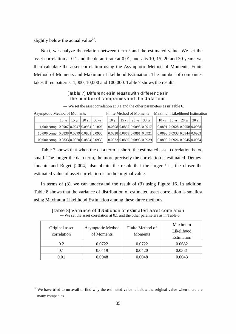
slightly below the actual value37.
Next, we analyze the relation between term t and the estimated value. We set the
asset correlation at 0.1 and the default rate at 0.01, and t is 10, 15, 20 and 30 years; we
then calculate the asset correlation using the Asymptotic Method of Moments, Finite
Method of Moments and Maximum Likelihood Estimation. The number of companies
takes three patterns, 1,000, 10,000 and 100,000. Table 7 shows the results.
[Table 7] Differences in results with differences in the number of companies and the data term
― We set the asset correlation at 0.1 and the other parameters as in Table 6.
Asymptotic Method of Moments Finite Method of Moments Maximum Likelihood Estimation 10 yr 15 yr 20 yr 30 yr 10 yr 15 yr 20 yr 30 yr 10 yr 15 yr 20 yr 30 yr
1,000 comp. 0.0907 0.0947 0.0984 0.1006 0.0808 0.0852 0.0893 0.0917 0.0891 0.0928 0.0950 0.0968
10,000 comp. 0.0838 0.0879 0.0901 0.0930 0.0828 0.0869 0.0891 0.0921 0.0898 0.0933 0.0944 0.0963
100,000 comp. 0.0833 0.0870 0.0894 0.0930 0.0832 0.0869 0.0893 0.0929 0.0898 0.0926 0.0945 0.0964
Table 7 shows that when the data term is short, the estimated asset correlation is too
small. The longer the data term, the more precisely the correlation is estimated. Demey,
Jouanin and Roget [2004] also obtain the result that the larger t is, the closer the
estimated value of asset correlation is to the original value.
In terms of (3), we can understand the result of (3) using Figure 16. In addition,
Table 8 shows that the variance of distribution of estimated asset correlation is smallest
using Maximum Likelihood Estimation among these three methods.
[Table 8] Variance of distribution of estimated asset correlation ― We set the asset correlation at 0.1 and the other parameters as in Table 6.
Original asset correlation
Asymptotic Method of Moments
Finite Method of Moments
Maximum Likelihood Estimation
0.2 0.0722 0.0722 0.0682 0.1 0.0419 0.0420 0.0381
0.01 0.0048 0.0048 0.0043
37 We have tried to no avail to find why the estimated value is below the original value when there are
many companies.
36
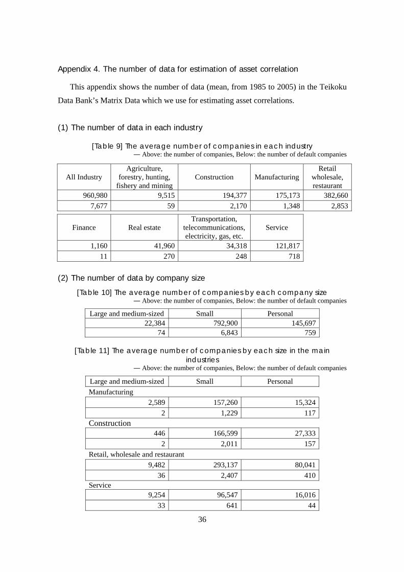
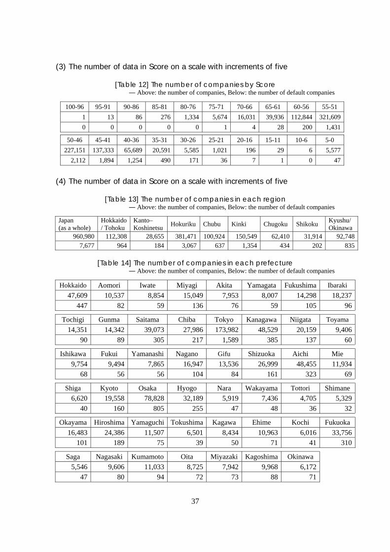
Appendix 4. The number of data for estimation of asset correlation
This appendix shows the number of data (mean, from 1985 to 2005) in the Teikoku
Data Bank’s Matrix Data which we use for estimating asset correlations.
(1) The number of data in each industry
[Table 9] The average number of companies in each industry ― Above: the number of companies, Below: the number of default companies
All Industry Agriculture,
forestry, hunting, fishery and mining
Construction Manufacturing Retail
wholesale, restaurant
960,980 9,515 194,377 175,173 382,6607,677 59 2,170 1,348 2,853
Finance Real estate Transportation,
telecommunications, electricity, gas, etc.
Service
1,160 41,960 34,318 121,817 11 270 248 718
(2) The number of data by company size
[Table 10] The average number of companies by each company size ― Above: the number of companies, Below: the number of default companies
Large and medium-sized Small Personal 22,384 792,900 145,697
74 6,843 759
[Table 11] The average number of companies by each size in the main industries
― Above: the number of companies, Below: the number of default companies
Large and medium-sized Small Personal Manufacturing
2,589 157,260 15,324 2 1,229 117
Construction 446 166,599 27,333
2 2,011 157 Retail, wholesale and restaurant
9,482 293,137 80,041 36 2,407 410
Service
9,254 96,547 16,016 33 641 44
37
(3) The number of data in Score on a scale with increments of five
[Table 12] The number of companies by Score ― Above: the number of companies, Below: the number of default companies
100-96 95-91 90-86 85-81 80-76 75-71 70-66 65-61 60-56 55-51 1 13 86 276 1,334 5,674 16,031 39,936 112,844 321,6090 0 0 0 0 1 4 28 200 1,431
50-46 45-41 40-36 35-31 30-26 25-21 20-16 15-11 10-6 5-0 227,151 137,333 65,689 20,591 5,585 1,021 196 29 6 5,577
2,112 1,894 1,254 490 171 36 7 1 0 47
(4) The number of data in Score on a scale with increments of five
[Table 13] The number of companies in each region ― Above: the number of companies, Below: the number of default companies
Japan (as a whole)
Hokkaido/ Tohoku
Kanto–Koshinetsu Hokuriku Chubu Kinki Chugoku Shikoku Kyushu/
Okinawa960,980 112,308 28,655 381,471 100,924 150,549 62,410 31,914 92,748
7,677 964 184 3,067 637 1,354 434 202 835
[Table 14] The number of companies in each prefecture ― Above: the number of companies, Below: the number of default companies
Hokkaido Aomori Iwate Miyagi Akita Yamagata Fukushima Ibaraki 47,609 10,537 8,854 15,049 7,953 8,007 14,298 18,237
447 82 59 136 76 59 105 96
Tochigi Gunma Saitama Chiba Tokyo Kanagawa Niigata Toyama 14,351 14,342 39,073 27,986 173,982 48,529 20,159 9,406
90 89 305 217 1,589 385 137 60
Ishikawa Fukui Yamanashi Nagano Gifu Shizuoka Aichi Mie 9,754 9,494 7,865 16,947 13,536 26,999 48,455 11,934
68 56 56 104 84 161 323 69
Shiga Kyoto Osaka Hyogo Nara Wakayama Tottori Shimane6,620 19,558 78,828 32,189 5,919 7,436 4,705 5,329
40 160 805 255 47 48 36 32
Okayama Hiroshima Yamaguchi Tokushima Kagawa Ehime Kochi Fukuoka16,483 24,386 11,507 6,501 8,434 10,963 6,016 33,756
101 189 75 39 50 71 41 310
Saga Nagasaki Kumamoto Oita Miyazaki Kagoshima Okinawa 5,546 9,606 11,033 8,725 7,942 9,968 6,172
47 80 94 72 73 88 71
38
References
Bluhm, C. and L. Overbeck, “Systematic risk in homogeneous credit portfolios,” Credit
Risk; Measurement, Evaluation and Management; Contributions to Economics,
Physica-Verlag/Springer, Heidelberg, Germany, 2003.
Carlos, J. and G. Cespedes, “Credit risk modelling and Basel II,” Algo Research
Quarterly, 5(1), 2002.
Chernih, A., S. Vanduffel and L. Henrard, “Asset correlations: A literature review and
analysis of the impact of dependent loss given defaults,” 2006. Available at
http://www.econ.kuleuven.be/insurance/pdfs/CVH-AssetCorrelations_v12.pdf
Demey, P., J. F. Jouanin and C. Roget, “Maximum likelihood estimates of default
correlations,” Risk, November, 2004, pp. 104–108.
Dietsch, M. and J. Petey, “Should SME exposures be treated as retail or corporate
exposures? A comparative analysis of default probabilities and asset correlations
in French and German SMEs,” Journal of Banking and Finance, 28, 2004, pp.
773–788.
Düllmann, K. and H. Scheule, “Determinants of the Asset Correlations of German
Corporations and Implications for Regulatory Capital,” Paper presented at the
10th Annual Meeting of the German Finance Association, 2003. Available at
http://www.cofar.uni-mainz.de/dgf2003/paper/paper53.pdf
Gordy, M., “A comparative anatomy of credit risk models,” Journal of Banking and
Finance, 24, 2000, pp. 119–149.
----------- and E. Heitfield, “Estimating Default Correlations from Short Panels of Credit
Rating Performance Data,” Working paper, Federal Reserve Board, 2002.
Available at http://elsa.berkeley.edu/~mcfadden/e242_f03/heitfield.pdf
Hamerle, A., T. Liebig and D. Rösch, “Credit Risk Factor Modeling and the Basel II
IRB Approach,” Deutsche Bundesbank Discussion Paper Series 2: Banking and
Financial Studies, No. 02, 2003.
Jakubik, P., “Does Credit Risk Vary with The Economic Cycles? The Case of Finland,”
Working Paper, Institute of Economic Studies, Faculty of Social Sciences,
39
Charles University in Prague, 2006. Available at
http://ies.fsv.cuni.cz/default/file/download/id/3869
Kitano, T., “Estimating Default Correlation from Historical Default Data – Maximum
Likelihood Estimation of Asset Correlation using Two-Factor Models – ,”
Transactions of the Operations Research Society of Japan, 50, 2007, pp. 42–67
(in Japanese, Deforuto Jisseki De-ta ni yoru Deforuto Izon Kankei no Suitei – 2
Fakuta-Model ni yoru Asetto Soukan no Saiyu Suitei).
Lopez, J. A., “The empirical relationship between average asset correlation, firm
probability of default and asset size,” Journal of Financial Intermediation, 13,
2004, pp. 265–283.
Merton, R., “On the pricing of corporate debt: The risk structure of interest rates,”
Journal of Finance, 29, 1974, pp. 449–470.