Embed Size (px)
Citation preview

Asset Management and Safety: A Performance Perspective
Sponsored byMidwest Transportation Consortium(MTC Project 2009-01)
Final ReportSeptember 2012

About MTCThe Midwest Transportation Consortium (MTC) is a Tier 1 University Transportation Center (UTC) that includes Iowa State University, the University of Iowa, and the University of Northern Iowa. The mission of the UTC program is to advance U.S. technology and expertise in the many disciplines comprising transportation through the mechanisms of education, research, and technology transfer at university-based centers of excellence. Iowa State University, through its Institute for Transportation (InTrans), is the MTC’s lead institution. This document is disseminated under the sponsorship of the Department of Transportation UTC Program in the interest of information exchange.
About CTREThe mission of the Center for Transportation Research and Education (CTRE) at Iowa State University is to develop and implement innovative methods, materials, and technologies for improving transportation efficiency, safety, and reliability while improving the learning environment of students, faculty, and staff in transportation-related fields.
Disclaimer NoticeThe contents of this report reflect the views of the authors, who are responsible for the facts and the accuracy of the information presented herein. The opinions, findings and conclusions expressed in this publication are those of the authors and not necessarily those of the sponsors.
The sponsors assume no liability for the contents or use of the information contained in this document. This report does not constitute a standard, specification, or regulation.
The sponsors do not endorse products or manufacturers. Trademarks or manufacturers’ names appear in this report only because they are considered essential to the objective of the document.
Iowa State University Non-Discrimination Statement Iowa State University does not discriminate on the basis of race, color, age, religion, national origin, sexual orientation, gender identity, genetic information, sex, marital status, disability, or status as a U.S. veteran. Inquiries can be directed to the Director of Equal Opportunity and Compliance, 3280 Beardshear Hall, (515) 294-7612.

Technical Report Documentation Page
1. Report No. 2. Government Accession No. 3. Recipient’s Catalog No.
MTC Project 2009-01
4. Title and Subtitle 5. Report Date
Asset Management and Safety: A Performance Perspective September 2012
6. Performing Organization Code
7. Authors(s) 8. Performing Organization Report No.
Jian Gao, Konstantina Gkritza, Omar Smadi, Neal R. Hawkins, Basak Aldemir
Bektas, and Inya Nlenanya
MTC Project 2009-01
9. Performing Organization Name and Address 10. Work Unit No. (TRAIS)
Center for Transportation Research and Education
Iowa State University
2711 South Loop Drive, Suite 4700
Ames, IA 50010-8664
11. Contract or Grant No.
12. Sponsoring Organization Name and Address 13. Type of Report and Period Covered
Midwest Transportation Consortium
Institute for Transportation
Iowa State University
2711 South Loop Drive, Suite 4700
Ames, IA 50010-8664
Final Report
14. Sponsoring Agency Code
15. Supplementary Notes
Visit www.intrans.iastate.edu for color pdfs of this and other research reports.
16. Abstract
Incorporating safety performance measures into asset management can assist transportation agencies in managing their aging assets
efficiently and improve system-wide safety. Past research has revealed the relationship between individual asset performance and safety,
but the relationship between combined measures of operational asset condition and safety performance has not been explored.
This project investigates the effect of pavement marking retroreflectivity and pavement condition on safety in a multi-objective manner.
Data on one-mile segments for all Iowa primary roads from 2004 through 2009 were collected from the Iowa Department of
Transportation and integrated using linear referencing.
An asset condition index (ACI) was estimated for the road segments by scoring and weighting individual components.
Statistical models were then developed to estimate the relationship between ACI and expected number of crashes, while accounting for
exposure (average daily traffic).
Finally, the researchers evaluated alternative treatment strategies for pavements and pavement markings using benefit-cost ratio
analysis, taking into account corresponding treatment costs and safety benefits in terms of crash reduction (number of crashes
proportionate to crash severity).
17. Key Words 18. Distribution Statement
asset condition index—asset economic analysis—AM data integration—crash
mitigation—operational road assets—pavement condition—pavement marking
retroreflectivity—pavement safety—road maintenance
No restrictions
19. Security Classification (of this
report)
20. Security Classification (of this
page)
21. No. of Pages 22. Price
Unclassified Unclassified 112 NA
Form DOT F 1700.7 (8-72) Reproduction of completed page authorized

ASSET MANAGEMENT AND SAFETY:
A PERFORMANCE PERSPECTIVE
Final Report
September 2012
Principal Investigator
Omar Smadi, PhD
Director and Research Scientist
Roadway Infrastructure Management and Operations Systems, Iowa State University
Co-Principal Investigators
Neal R. Hawkins, PE
Director
Center for Transportation Research and Education, Iowa State University
Konstantina Gkritza, PhD
Assistant Professor of Civil, Construction, and Environmental Engineering
Center for Transportation Research and Education, Iowa State University
Postdoctoral Research Associate
Basak Aldemir Bektas, PhD
Center for Transportation Research and Education, Iowa State University
Graduate Research Assistant
Jian Gao
Authors
Jian Gao, Konstantina Gkritza, Omar Smadi, Neal R. Hawkins,
Basak Aldemir Bektas, Inya Nlenanya
Sponsored by
the Midwest Transportation Consortium
(MTC Project 2009-01)
A report from
Center for Transportation Research and Education
Iowa State University
2711 South Loop Drive, Suite 4700
Ames, IA 50010-8664
Phone: 515-294-8103 Fax: 515-294-0467
www.intrans.iastate.edu

v
TABLE OF CONTENTS
ACKNOWLEDGMENTS ............................................................................................................. xi
EXECUTIVE SUMMARY ......................................................................................................... xiii
Key Findings .......................................................................................................................... xiii
Recommendations for Future Research ................................................................................. xiv
1. INTRODUCTION .................................................................................................................... 1
1.1 Problem Statement .............................................................................................................. 1
1.2 Research Objectives and Tasks........................................................................................... 2
2. LITERATURE REVIEW ......................................................................................................... 4
2.1 Asset Management .............................................................................................................. 4
2.2 Review of Select Asset Performance and Safety Measures ............................................... 8
3. DATA DESCRIPTION .......................................................................................................... 11
3.1 Crash Data......................................................................................................................... 11
3.2 Pavement Condition Data ................................................................................................. 12
3.3 Pavement Marking Retroreflectivity Data ........................................................................ 13
3.4 Linear Referencing System (LRS) .................................................................................... 14
4. DATA INTEGRATION ......................................................................................................... 15
4.1 Data Integration Concepts in Asset Management............................................................. 15
4.2 Route Milepost-Based Integration .................................................................................... 17
4.3 Summary ........................................................................................................................... 19
5. ESTIMATION OF ASSET CONDITION ............................................................................. 20
5.1 Literature Review ............................................................................................................. 20
5.2 ACI Estimation ................................................................................................................. 22
5.3 Summary ........................................................................................................................... 25
6. STATISTICAL ANALYSIS OF CRASH FREQUENCY ..................................................... 26
6.1 Descriptive Statistics......................................................................................................... 26
6.2 Statistical Analysis ............................................................................................................ 32
6.3 Summary ........................................................................................................................... 37
7. EVALUATION OF ASSET TREATMENT STRATEGIES ................................................. 38
7.1 Goal of the Evaluation ...................................................................................................... 38
7.2 Treatment Alternatives ..................................................................................................... 38
7.3 Relative ACI Improvement and Depreciation Rate .......................................................... 40
7.4 Identifying Costs and Benefits .......................................................................................... 41
7.5 Single-Year Benefit-Cost Ratio (BCR) Analysis ............................................................. 42
7.6 Five-Year Net Present Value (NPV) Analysis ................................................................. 44
7.7 Summary ........................................................................................................................... 48
8. CONCLUSIONS AND RECOMMENDATIONS ................................................................. 49
8.1 Research Summary ........................................................................................................... 49
8.2 Key Findings ..................................................................................................................... 49
vi
8.3 Study Limitations .............................................................................................................. 50
8.4 Recommendations for Future Research ............................................................................ 51
REFERENCES ............................................................................................................................. 53
APPENDIX A. STATISTICAL ANALYSIS RESULTS ............................................................ 57
APPENDIX B. ECONOMIC ANALYSIS ................................................................................... 62
Five-Year Net Present Value (NPV) Analysis ....................................................................... 63
vii
LIST OF FIGURES
Figure 2.1. Components of an asset management system (Smith 2005) ........................................ 5
Figure 2.2. Overall framework for asset management (Falls, et al. 2001) ..................................... 6
Figure 3.1. Distribution of crashes per mile ................................................................................. 12
Figure 3.2. Sample Iowa primary roads pavement condition data map........................................ 13
Figure 3.3. Sample Iowa primary roads pavement marking retroreflectivity data map ............... 14
Figure 5.1. ACI sector and sub-index weighting layout ............................................................... 24
Figure 6.1. Histogram of ACI ....................................................................................................... 26
Figure 6.2. Distribution of ACI by year ........................................................................................ 27
Figure 6.3. Histogram of ADT ...................................................................................................... 28
Figure 6.4. Histogram of log(ADT) .............................................................................................. 29
Figure 6.5. Distribution of log(ADT) by year............................................................................... 29
Figure 6.6. Histogram of number of crashes................................................................................. 30
Figure 6.7. Distribution of number of crashes by year ................................................................. 31
Figure 6.8. Predicted crash frequency versus ACI ....................................................................... 35
Figure 7.1. Crash trends before and after treatment...................................................................... 45
Figure 7.2. NPV for pavement condition group alternatives by ACI range ................................. 46
Figure 7.3. NPV for pavement marking group alternatives by ACI range ................................... 47
Figure B.1. Reconstruction NPV in Range 1 ................................................................................ 63
Figure B.2. Major rehabilitation NPV in Range 1 ........................................................................ 64
Figure B.3. Minor rehabilitation NPV in Range 1 ........................................................................ 65
Figure B.4. Paint marking NPV in Range 1.................................................................................. 66
Figure B.5. Durable marking NPV in Range 1 ............................................................................. 67
Figure B.6. Tape marking NPV in Range 1 .................................................................................. 68
Figure B.7. Reconstruction NPV in Range 2 ................................................................................ 69
Figure B.8. Major rehabilitation NPV in Range 2 ........................................................................ 70
Figure B.9 Minor rehabilitation NPV in Range 2 ......................................................................... 71
Figure B.10. Paint marking NPV in Range 2................................................................................ 72
Figure B.11. Durable marking NPV in Range 2 ........................................................................... 73
Figure B.12. Tape marking NPV in Range 2 ................................................................................ 74
Figure B.13. Reconstruction NPV in Range 3 .............................................................................. 75
Figure B.14. Major rehabilitation NPV in Range 3 ...................................................................... 76
Figure B.15. Minor rehabilitation NPV in Range 3 ...................................................................... 77
Figure B.16. Paint marking NPV in Range 3................................................................................ 78
Figure B.17. Durable marking NPV in Range 3 ........................................................................... 79
Figure B.18. Tape marking NPV in Range 1 ................................................................................ 80
Figure B.19. Reconstruction NPV in Range 4 .............................................................................. 81
Figure B.20. Major rehabilitation NPV in Range 4 ...................................................................... 82
Figure B.21. Minor rehabilitation NPV in Range 4 ...................................................................... 83
viii
Figure B.22. Paint marking NPV in Range 4................................................................................ 84
Figure B.23. Durable marking NPV in Range 4 ........................................................................... 85
Figure B.24. Tape marking NPV in Range 1 ................................................................................ 86
Figure B.25. Reconstruction NPV in Range 5 .............................................................................. 87
Figure B.26. Major rehabilitation NPV in Range 5 ...................................................................... 88
Figure B.27. Minor rehabilitation NPV in Range 5 ...................................................................... 89
Figure B.28. Paint marking NPV in Range 5................................................................................ 90
Figure B.29. Durable marking NPV in Range 5 ........................................................................... 91
Figure B.30. Tape marking NPV in Range 5 ................................................................................ 92
Figure B.31. Reconstruction NPV in Range 6 .............................................................................. 93
Figure B.32. Major rehabilitation NPV in Range 6 ...................................................................... 94
Figure B.33. Minor rehabilitation NPV in Range 6 ...................................................................... 95
Figure B.34. Paint marking NPV in Range 6................................................................................ 96
Figure B.35. Durable marking NPV in Range 6 ........................................................................... 97
Figure B.36. Tape marking NPV in Range 6 ................................................................................ 98
ix
LIST OF TABLES
Table 3.1. Descriptive statistics (variable: crashes per mile) ........................................................ 11
Table 5.1. Summary of weighting methods .................................................................................. 20
Table 5.2. Score matrix of ACI sub-indices ................................................................................. 23
Table 6.1. Descriptive statistics for the ACI ................................................................................. 26
Table 6.2. Descriptive statistics for ADT ..................................................................................... 27
Table 6.3. Descriptive statistics of Log(ADT) .............................................................................. 28
Table 6.4. Descriptive statistics for number of crashes ................................................................ 30
Table 6.5. Correlation matrix ........................................................................................................ 31
Table 6.6. Negative binomial model estimation results ................................................................ 33
Table 6.7. Sensitivity analysis of weights ..................................................................................... 33
Table 6.8. Statistical model estimation results for sensitivity study ............................................. 34
Table 6.9. Transferability test estimation for ACI ranges ............................................................ 36
Table 6.10. Summary of separate negative binomial models ....................................................... 36
Table 7.1. Attributes of treatment alternatives .............................................................................. 41
Table 7.2. Iowa crash costs in 2007 .............................................................................................. 42
Table 7.3. Distribution of crashes by severity .............................................................................. 42
Table 7.4. NPV and BCR of treatment alternatives one year after implementation ..................... 43
Table 7.5. Reduction in crash frequency and NPV for major rehabilitation on segments with
1.5 < ACI ≤ 2.00 ........................................................................................................................... 44
Table B.1. Reduced number of crashes by severity ...................................................................... 62
Table B.2. Benefit from reduced numbers of crashes ................................................................... 62
Table B.3. Reconstruction NPV in Range 1 ................................................................................. 63
Table B.4. Major rehabilitation NPV in Range 1 ......................................................................... 64
Table B.5. Minor rehabilitation NPV in Range 1 ......................................................................... 65
Table B.6. Paint marking NPV in Range 1 ................................................................................... 66
Table B.7. Durable marking NPV in Range 1 .............................................................................. 67
Table B.8. Tape marking NPV in Range 1 ................................................................................... 68
Table B.9. Reconstruction NPV in Range 2 ................................................................................. 69
Table B.10. Major rehabilitation NPV in Range 2 ....................................................................... 70
Table B.11. Minor rehabilitation NPV in Range 2 ....................................................................... 71
Table B.12. Paint marking NPV in Range 2 ................................................................................. 72
Table B.13. Durable marking NPV in Range 2 ............................................................................ 73
Table B.14. Tape marking NPV in Range 2 ................................................................................. 74
Table B.15. Reconstruction NPV in Range 3 ............................................................................... 75
Table B.16. Major rehabilitation NPV in Range 3 ....................................................................... 76
Table B.17. Minor rehabilitation NPV in Range 3 ....................................................................... 77
Table B.18. Paint marking NPV in Range 3 ................................................................................. 78
Table B.19. Durable marking NPV in Range 3 ............................................................................ 79
x
Table B.20. Tape marking NPV in Range 1 ................................................................................. 80
Table B.21. Reconstruction NPV in Range 4 ............................................................................... 81
Table B.22. Major rehabilitation NPV in Range 4 ....................................................................... 82
Table B.23. Minor rehabilitation NPV in Range 4 ....................................................................... 83
Table B.24. Paint marking NPV in Range 4 ................................................................................. 84
Table B.25. Durable marking NPV in Range 4 ............................................................................ 85
Table B.26. Tape marking NPV in Range 4 ................................................................................. 86
Table B.27. Reconstruction NPV in Range 5 ............................................................................... 87
Table B.28. Major rehabilitation NPV in Range 5 ....................................................................... 88
Table B.29. Minor rehabilitation NPV in Range 5 ....................................................................... 89
Table B.30. Paint marking NPV in Range 5 ................................................................................. 90
Table B.31. Durable marking NPV in Range 5 ............................................................................ 91
Table B.32. Tape marking NPV in Range 5 ................................................................................. 92
Table B.33. Reconstruction NPV in Range 6 ............................................................................... 93
Table B.34. Major rehabilitation NPV in Range 6 ....................................................................... 94
Table B.35. Minor rehabilitation NPV in Range 6 ....................................................................... 95
Table B.36. Paint marking NPV in Range 6 ................................................................................. 96
Table B.37. Durable marking NPV in Range 6 ............................................................................ 97
Table B.38. Tape marking NPV in Range 6 ................................................................................. 98

xi
ACKNOWLEDGMENTS
The researchers would like to thank the Midwest Transportation Consortium for sponsoring this
research. The researchers also want to acknowledge the Iowa Department of Transportation for
providing data to support this project.

xiii
EXECUTIVE SUMMARY
Incorporating safety performance measures into asset management can assist transportation
agencies in managing their aging assets efficiently and improve system-wide safety. Past
research has revealed the relationship between individual asset performance and safety, but the
relationship between combined measures of operational asset condition and safety performance
has not been explored.
This project investigates the effect of pavement marking retroreflectivity and pavement condition
on safety in a multi-objective manner. Data on one-mile segments for all Iowa primary roads
from 2004 through 2009 were collected from the Iowa Department of Transportation and
integrated using linear referencing.
An asset condition index (ACI) was estimated for the road segments by scoring and weighting
individual components.
Statistical models were then developed to estimate the relationship between ACI and expected
number of crashes, while accounting for exposure.
Finally, the researchers evaluated alternative treatment strategies for pavements and pavement
markings using benefit-cost ratio analysis, taking into account corresponding treatment costs and
safety benefits in terms of crash reduction (number of crashes proportionate to crash severity).
Key Findings
Estimation of Asset Condition Index
The ACI was developed as a simple, convenient, and easy-to-understand indicator for
representing the overall physical asset condition of a roadway segment and assisting agencies in
decision-making for pavement preservation and maintenance activities.
The researchers developed a step-by-step methodology for calculating the unique condition
index using multiple asset condition measures. The methodology involved scaling and weighting
asset condition components, such as pavement condition and pavement retroreflectivity, as well
as their subcomponents. The resulting ACI values range from 1, indicating poor condition, to°3,
indicating good condition.
Statistical Analysis
Negative binomial models were estimated to predict the relationship between crash frequency
and ACI, while accounting for exposure. The estimation results indicated that the higher the ACI
of a roadway segment, the lower the expected number of crashes.
xiv
In addition, the researchers found that separate negative binomial models for different ACI
ranges explain the relationship among crash frequency, ACI, and exposure (average daily traffic
or ADT) better than a single model. The impact of ACI on crash frequency for roadway
segments with an ACI lower or equal to 1.5 was greater than that for roadway segments with an
ACI higher than 1.5.
Economic Analysis
Both short-term and long-term safety benefits in terms of crash reduction along with treatment
costs were estimated for six alternative treatment strategies via a single-year benefit-cost ratio
(BCR) analysis and a five-year net present value (NPV) analysis.
Minor rehabilitation and use of durable pavement marking materials are recommended as more
cost-effective treatment alternatives in the short-term. In the long-term, the same
recommendation holds for segments with an ACI higher than 2.0. For segments with an ACI
lower than 1.5, major rehabilitation and tape marking are recommended.
Study Limitations
The limitations pertaining to this study are discussed in the Conclusions and Recommendations.
Recommendations for Future Research
To understand the relationship between asset performance and safety performance better, the
following recommendations are offered for future studies.
Analysis of future data: A longer study period for the database developed in this study
would help to define the relationship between asset performance and safety
performance more accurately. A further process of relating crashes to asset
performance measures, based on crash reasons, is expected to improve the accuracy
of the research.
Replication of this study in other states: A replication of this study in other states
would help verify the results and/or identify differences among states. Similar data
resources would be necessary.
Consideration of additional asset performance measures: Only pavement condition
and pavement marking performance were included in this study. Additional asset
conditions that could be considered in future work include sign inventory, lighting
inventory, rumble strip inventory, or guardrail locations.

1
1. INTRODUCTION
1.1 Problem Statement
Asset management (AM) is an efficient approach to manage the performance and investment in
roadway infrastructure. AM concepts, principles, and performance measures have received
increasing attention from transportation agencies and transportation leaders in the US and abroad
in the last two decades.
AM concepts and tools utilize tradeoff analysis and multi-criteria decision making by
incorporating system-wide costs and benefits of alternative strategies.
The Iowa Department of Transportation (DOT) has a rich history in the implementation of
infrastructure management systems, such as pavement, bridge, and pavement marking
management systems, and, consequently, has comprehensive historic data for different assets.
Recently, the Iowa DOT started its own asset management implementation process. This
decision was made, not only because of the economic recession, but also due to the desire for a
systematic, efficient, and critical methodology for fiscal investment.
In addition, as a state with a low crash rate and one of the best safety databases in the country,
the Iowa DOT is interested in assessing safety benefits or the effect on safety of any project or
management system.
In 2011, the total fatalities on Iowa roadways were 364, which is the lowest number of deaths
since 1944, and the crash rate has dropped to less than one fatality for every 10,000 registered
vehicles (Iowa DOT 2012), which is lower than the nationwide average (about 1.2 fatalities per
10,000 registered vehicles in 2009) (NHTSA 2009).
While past research has revealed the relationship between individual asset performance (such as
pavement condition and pavement marking retroreflectivity) and safety, the relationship between
combined measures of operational asset condition and safety performance has not been fully
examined.
Furthermore, to date, the impact of alternative strategies on safety has not been included in the
decision-making framework. Therefore, a need exists to develop a methodology for investigating
the relationship between asset performance and safety and further investigate the feasibility of
developing a methodology to prioritize safety improvements based on this relationship.
Incorporating safety performance measures into asset management can assist agencies in
managing their aging assets efficiently and improve safety, system-wide.
2
1.2 Research Objectives and Tasks
The objectives of this study were as follows:
Develop a methodology for estimating an index that represents overall physical asset
condition on a roadway segment
Investigate the effect of asset condition on safety and develop a methodology to
prioritize safety improvements based on asset condition
To achieve these objectives, the following tasks were conducted.
Task 1: Review of Literature
The literature review included the overview of asset management, the potential benefits of
integrating safety into asset management, and the review of selected asset performance and
safety measures.
Task 2: Descriptive Data Analysis
The datasets from different management systems, such as the Iowa DOT Pavement Management
Information System (PMIS) and Iowa Pavement Marking Management System (IPMMS) are
introduced, summarized, and interpreted using descriptive analysis techniques and geographic
information systems (GIS). The Iowa DOT crash datasets were also used in this study.
Task 3: Integration of different data sets
The collected datasets were integrated using the Iowa DOT linear referencing system (LRS).
Task 4: Estimation of Asset Condition Index
An ACI was developed as a simple, convenient, and understandable indicator for representing
the overall physical asset condition of a roadway segment. The step-by-step methodology for
calculating a unique condition index of multiple asset conditions can assist agencies in
monitoring asset condition using a convenient indicator.
Task 5: Investigation of Relationship between Asset Performance and Safety Performance
The relationship between crash frequency and ACI was investigated, taking into account traffic
exposure (average daily traffic or ADT). Statistical analyses were conducted to select appropriate
models to estimate the relationship between ACI, exposure, and number of crashes. Separate
models were developed for ACI ranges as explained later in this report.
3
Task 6: Evaluation of Different Asset Treatment Strategies
A single-year benefit-cost ratio (BCR) analysis and five-year net present value (NPV) analysis
were conducted. Both short-term and long-term safety benefits and treatment costs were
estimated for six alternative treatment strategies. Recommendations based on the analysis are
presented as well.
Task 7: Conclusions and Recommendations
Based on the work conducted in the previous tasks, some concluding remarks and
recommendations are offered. Additional research needs for future studies were also identified.

4
2. LITERATURE REVIEW
2.1 Asset Management
2.1.1 Definition of Asset Management
AM is a systematic process of maintaining, upgrading, and operating physical assets cost-
effectively (Office of Asset Management 1999). AM combines engineering principles with
business practice and economic rationale for resource allocation and utilization with the goal of
better decision-making based on quality information and well-defined objectives. (OECD 2001).
The Asset Management Primer from the Federal Highway Administration (FHWA) indicates
that AM is a decision-making framework, which is guided by goals of performance (Office of
Asset Management 1999). AM should help highway agencies develop improvement plans and
budget allocation policies to maintain, repair, or replace infrastructure cost-effectively and at the
appropriate time (Haas 2001).
AM also encompasses principles of engineering, engineering policies, economics and business
management, and provides tools for both short-term and long-term planning and decision-
making. Business practices from both the public and private sectors are taken into account in an
AM system (Falls, et al. 2001).
According to the FHWA, an AM system should include 13 components, as follows (Office of
Asset Management 1999):
Strategic goals
Inventory of assets
Valuation of assets
Quantitative condition and performance measures
Measures of how well strategic goals are being met
Usage information
Performance-prediction capabilities
Relational databases to integrate individual management systems
Consideration of qualitative issues
Links to the budget process
Engineering and economic analysis tools
Useful outputs, effectively presented
Continuous feedback procedures
These components could be grouped into five major functions (Krugler, et al. 2006):
Basic information
Performance measures

5
Needs analysis
Program analysis
Program delivery
Figure 2.1 shows the comprehensive relationship between the five functions and the 13 basic
components of AM.
Figure 2.1. Components of an asset management system (Smith 2005)
This is a simplified and recommended flow of the system that agencies can modify depending on
their own data history and availability, resources, desired level of service, and so forth.
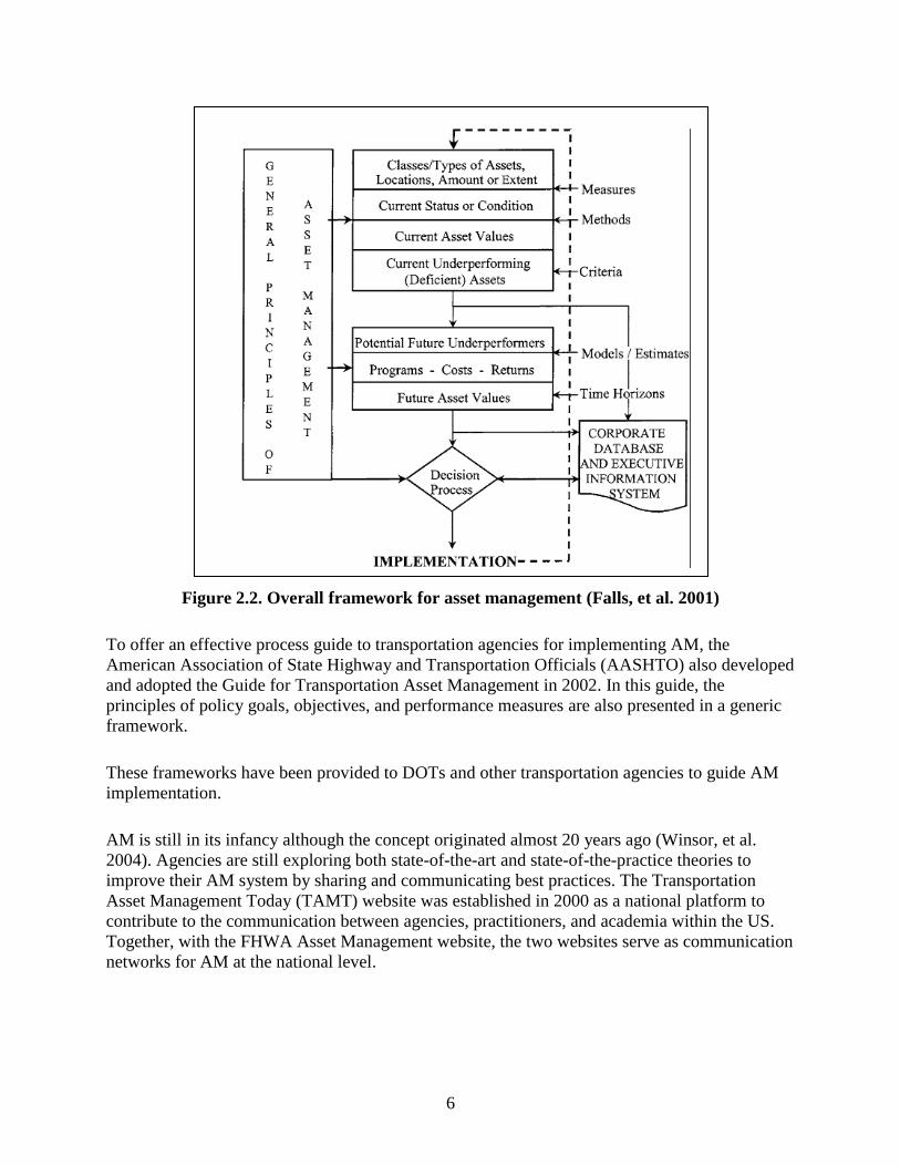
In 2002, the Transportation Association of Canada presented an overall framework of AM as
shown in Figure 2.2.
6
Figure 2.2. Overall framework for asset management (Falls, et al. 2001)
To offer an effective process guide to transportation agencies for implementing AM, the
American Association of State Highway and Transportation Officials (AASHTO) also developed
and adopted the Guide for Transportation Asset Management in 2002. In this guide, the
principles of policy goals, objectives, and performance measures are also presented in a generic
framework.
These frameworks have been provided to DOTs and other transportation agencies to guide AM
implementation.
AM is still in its infancy although the concept originated almost 20 years ago (Winsor, et al.
2004). Agencies are still exploring both state-of-the-art and state-of-the-practice theories to
improve their AM system by sharing and communicating best practices. The Transportation
Asset Management Today (TAMT) website was established in 2000 as a national platform to
contribute to the communication between agencies, practitioners, and academia within the US.
Together, with the FHWA Asset Management website, the two websites serve as communication
networks for AM at the national level.
7
2.1.2 AM and Pavement Management
For many years, state DOTs have viewed AM as two separate systems: pavement management
and bridge management (Krugler, et al. 2006). While the general AM framework is similar to the
network-level programming of a pavement management system (Haas and Chairman, 2001),
individual AM systems in no way replace AM (Office of Asset Management 1999). AM applies
to all infrastructure assets beyond pavements and bridges.
Pavement management systems were the first systems implemented to manage assets, so
agencies have the most experience with them. This experience can guide agencies in
implementing AM principles to other infrastructure assets. Bridge management systems are
common AM systems but with a relatively shorter history.
2.1.3 Potential Benefits of Integrating Safety Elements in AM
The primary benefits of AM implementation are savings in human lives, as well as resources,
which are very important considerations for all road agencies. More specific benefits are
summarized as follows (FHWA 2005):
Better resource allocation decisions. AM techniques and tools help agencies to
optimize the resource expenditure plans for asset maintenance, upgrades, and
operations rationally. The rationale for expenditure decisions can be provided easily
to upper management, other decision makers, the public, and the media.
Simplified economic processes and cost saving. AM tracks costs. This cost tracking
could support the preparation of more detailed and accurate cost estimates and budget
plans. In addition, with better information, more accurate cost data, more timely
decisions, and other efficiency improvement plans, agencies could reduce the costs of
maintenance, upgrade, and operating of assets.
Improving data access. AM requires creating a complete, timely, and accurate
database that can be accessed quickly. The inventory of assets, their location,
condition, maintenance and repair history, and other relevant information can be
shared in real time and updated continually. Easy access to information helps
managers, executives, policymakers, and other relevant officers of an agency to make
better decisions.
Improved data clarity and consistency. The consistency of the shared standard
definitions, measurements, and formats improve the accuracy and reliability of data.
Improved safety through faster response to customer service requests. Consideration
of the safety of signs, lightings, pavement markings, and other roadway safety
elements account for a significant part of the interaction between transportation
agencies and users. Quicker access to data about the safety elements facilitates faster
customer service and makes roads safer.
Reduced duplication effort. Because central and regional offices can share
information, duplication of effort (for example, multiple data entry) is reduced or
eliminated.
8
2.2 Review of Select Asset Performance and Safety Measures
The literature review revealed that very limited research has focused on the relationship between
asset physical performance and safety performance. However, previous studies have been
conducted for selected elements, such as pavement condition, pavement marking
retroreflectivity, sign condition, and lighting, and their relationships to safety. Based on the
previous findings, each element has a different effect on safety.
The following research sections describe the existing literature on the relationship between asset
condition and safety.
2.2.1 Pavement Condition
Among studies, pavement condition was found to have significant effect on highway safety, and
the magnitude of the effect could vary depending on the selected pavement condition measure
and the confidence level of the analysis.
Few statewide studies on pavement distress and safety existed before 1990 because the data
collection methodologies were not developed well enough before then. Studies conducted in
recent years can be divided, basically, into experimental studies and simulation studies.
However, research studies about safety and pavement distress are still few, and most of them
focus on a single type of distress, such as rutting or roughness, as it relates to safety (Chan, et al.
2008).
The severity of crashes related to pavement edge drop-off depends on several factors, such as
speed, shoulder geometry, and lane width (Ivey, et al. 1990). Start et al. 1998 found that
pavement rutting of 0.3 in. or deeper would significantly increase crash rate (Start, Kim and Berg
1998).
Pavement roughness can also be measured by the International Roughness Index (IRI) or Riding
Number (RN) (Chan, et al. 2008). IRI has become the standard for assessing pavement surface
roughness in recent years. IRI is based on a quarter-car model traveling the pavement surface at a
constant speed.
IRI has been proven to explain phenomena such as pavement performance and pavement
deterioration satisfactorily (Surface Properties–Vehicle Interaction Committee 2009). The
transportation department of New Zealand conducted a study on crashes from 1997 to 2002. The
results indicated that crash rate does not have a significant relationship with both IRI and rutting
depth (Cenek and Davies 2002).
Conversely, previous work has shown that the higher the IRI, the lower the brake force
(Nakatsuji, et al. 1990), the higher the difference of friction on each tire (Chan, et al. 2008), and
the higher the probability of crashes (Burns 1981).
9
In addition, the relationship between the Present Serviceability Index (PSI) and crash rates on
rural roads was found to have a significant effect on single- and multiple-vehicle crash rates, but
no statistical influence on the total crash rate (Al-Masaeid 1997). PSI has been indicated as the
second most important safety factor for rural two-lane highways and the fifth most important
factor for rural multilane highways (Karlaftis and Golias 2002).
A study in Victoria, Australia examined the relationship between road surface characteristics,
such as macrotexture, rutting, and roughness, and safety (Cairney and Bennett 2008). The study
found that the higher the macrotexture of the pavement, or the better the condition, the lower the
crash rate. Furthermore, the study showed that crash rate decreases, following an exponential
distribution, when macrotexture increases.
This study also found that the relationship between rutting and crash rate could be expressed by a
power function, although with a relatively low confidence factor, which could suggest that the
depth of the rutting might not have a significant or direct effect on the crash rate. On the other
hand, the relationship between roughness and crash rate was found to follow a power function
almost exactly, and the authors concluded that roughness significantly affects crash rates.
In terms of classification, for joint faulting, the Washington State DOT (WSDOT) set the
limitation as 2.5 mm and 4 mm as acceptable and maintenance required thresholds, respectively
(Pavement Interactive 2011), and NCHRP Synthesis 334 suggests pavement faulting depth of 2.5
mm as acceptable and 5.0 mm or higher as a poor level (McGhee 2004).
For rutting depth, 6 mm and 15 mm are common criterion for good and poor condition
thresholds among agencies, such as the California DOT (Caltrans) and MaineDOT (Gallivan
2003) (MaineDOT 2006).
In terms of friction, the NCHRP Guide for Pavement Friction indicated that road segments with a
friction number (FN) of 60 would be considered as good (Hall, et al. 2009), while the NCHRP
Synthesis 291 report suggested that FN lower than 35 should be considered as poor and
maintenance could be performed (Henry 2000).
2.2.2 Pavement Marking Retroreflectivity
The review of the limited studies on the effect of pavement marking retroreflectivity on safety
revealed mixed findings. A National Cooperative Highway Research Program (NCHRP) study
conducted by iTRANS Consulting of Ontario, Canada found no significant effect of pavement
marking and marker retroreflectivity on crash rate (Harrigan 2006). More specifically, the
presence and visibility of markings are important to drivers, but whether the markings have high
retroreflectivity or relatively low retroreflectivity is less important with respect to safety.
One hypothesis is that drivers compensate by reducing their speed under lower visibility
conditions, and maintain higher speeds under higher visibility (Bahar, et al. 2006). However,
Smadi et al. (2008) conducted a three-year statistical analysis of pavement marking
10
retroreflectivity data and crash rates that were collected by the Iowa DOT on all Iowa primary
roads and the study indicated that the higher the retroreflectivity of pavement markings, the
lower the relative crash probability, regardless of traffic volume. This result applied to both
yellow and white edge lines on either freeways or two-lane roads (Smadi, et al. 2008).
The minimum levels of marking retroreflectivity have been studied as well. The 3M Company
conducted a study where subjects drove a test road marked similarly to one side of a four-lane
freeway in 1986. A minimum retroreflective value of 100 mcd/m2/lux was suggested as a
conservative recommendation due to instrument variability (Ethen and Woltman 1986).
The Minnesota DOT (MnDOT) sponsored a 1998 study that used a sample of drivers in the state
to assess minimum pavement marking retroreflectivity. The study found that 90 percent of the
participants rated yellow markings with a retroreflectivity of 100 mcd/m2/lux as acceptable. In
addition, the researchers found that the acceptability ratings of the pavement markings increased
dramatically as the retroreflectivity increased from 0 to 120 mcd/m2/lux, much less as the
retroreflectivity increased from 120 to 200 mcd/m2/lux, and almost none as the retroreflectivity
increased beyond 200 mcd/m2/lux. The researchers recommended that MnDOT use 120
mcd/m2/lux as the threshold between acceptable and unacceptable pavement marking
retroreflectivity in its pavement marking maintenance program (Loetterle, et al. 2000).
The NCHRP Synthesis 306 report states that minimum retroreflectivity of yellow marking is
100 mcd/m2/lux and 150 mcd/m
2/lux for white marking. Also, any pavement marking
retroreflectivity beyond 200 mcd/m2/lux should be considered as in good level (Miglets and
Graham 2002).
11
3. DATA DESCRIPTION
The data sources that were used in this project include Iowa DOT crash data, pavement condition
data, pavement marking retroreflectivity data, and other inventory data from their Geographic
Information Management System (GIMS) database.
The following sections describe each data source in detail.
3.1 Crash Data
The Iowa DOT collects information on crashes that occur on all Iowa public roads. However,
crashes that result in less than $1,500 in property damage only (PDO) are not required to be
reported in Iowa.
This study used crash data for Iowa primary roads from 2004 through 2009. These data include
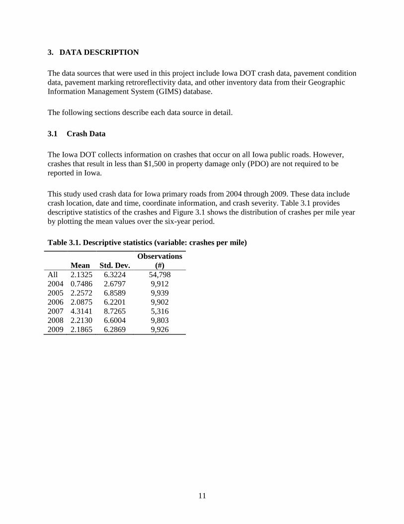
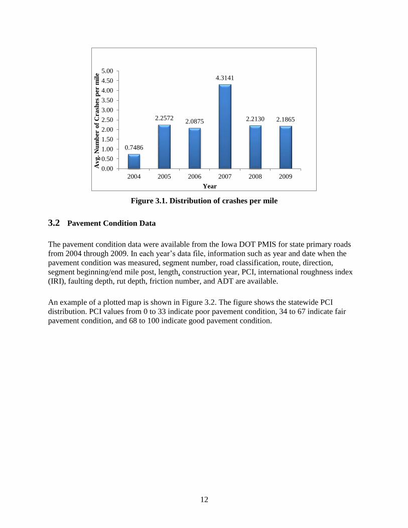
crash location, date and time, coordinate information, and crash severity. Table 3.1 provides
descriptive statistics of the crashes and Figure 3.1 shows the distribution of crashes per mile year
by plotting the mean values over the six-year period.
Table 3.1. Descriptive statistics (variable: crashes per mile)
Mean Std. Dev.
Observations
(#)
All 2.1325 6.3224 54,798
2004 0.7486 2.6797 9,912
2005 2.2572 6.8589 9,939
2006 2.0875 6.2201 9,902
2007 4.3141 8.7265 5,316
2008 2.2130 6.6004 9,803
2009 2.1865 6.2869 9,926
12
Figure 3.1. Distribution of crashes per mile
3.2 Pavement Condition Data
The pavement condition data were available from the Iowa DOT PMIS for state primary roads
from 2004 through 2009. In each year’s data file, information such as year and date when the
pavement condition was measured, segment number, road classification, route, direction,
segment beginning/end mile post, length, construction year, PCI, international roughness index
(IRI), faulting depth, rut depth, friction number, and ADT are available.
An example of a plotted map is shown in Figure 3.2. The figure shows the statewide PCI
distribution. PCI values from 0 to 33 indicate poor pavement condition, 34 to 67 indicate fair
pavement condition, and 68 to 100 indicate good pavement condition.
0.7486
2.2572 2.0875
4.3141
2.2130 2.1865
0.00
0.50
1.00
1.50
2.00
2.50
3.00
3.50
4.00
4.50
5.00
2004 2005 2006 2007 2008 2009
Av
g. N
um
ber
of
Cra
shes
per
mil
e
Year

13
Figure 3.2. Sample Iowa primary roads pavement condition data map
3.3 Pavement Marking Retroreflectivity Data
Pavement marking retroreflectivity data were available from 2004 through 2010 using the
IPMMS. The Iowa DOT collects pavement marking retroreflectivity on state primary roads twice
each year, in the fall and spring.
The data fields include route information, milepost, line type, direction, retroreflectivity value,
date when the measurements were taken, material type, marking length (five-mile segmentation),
and coordinate information.
In addition to the seasonal databases, the repainting database was also available and used. Every
year, the Iowa DOT re-strips low retroreflectivity markings from April to September, so separate
databases indicating repainted markings information were generated. The availability for this
repainting database was 2004 through 2008, including painting dates, length, beginning/end
mileposts, directions, retroreflectivity value, and other related information.
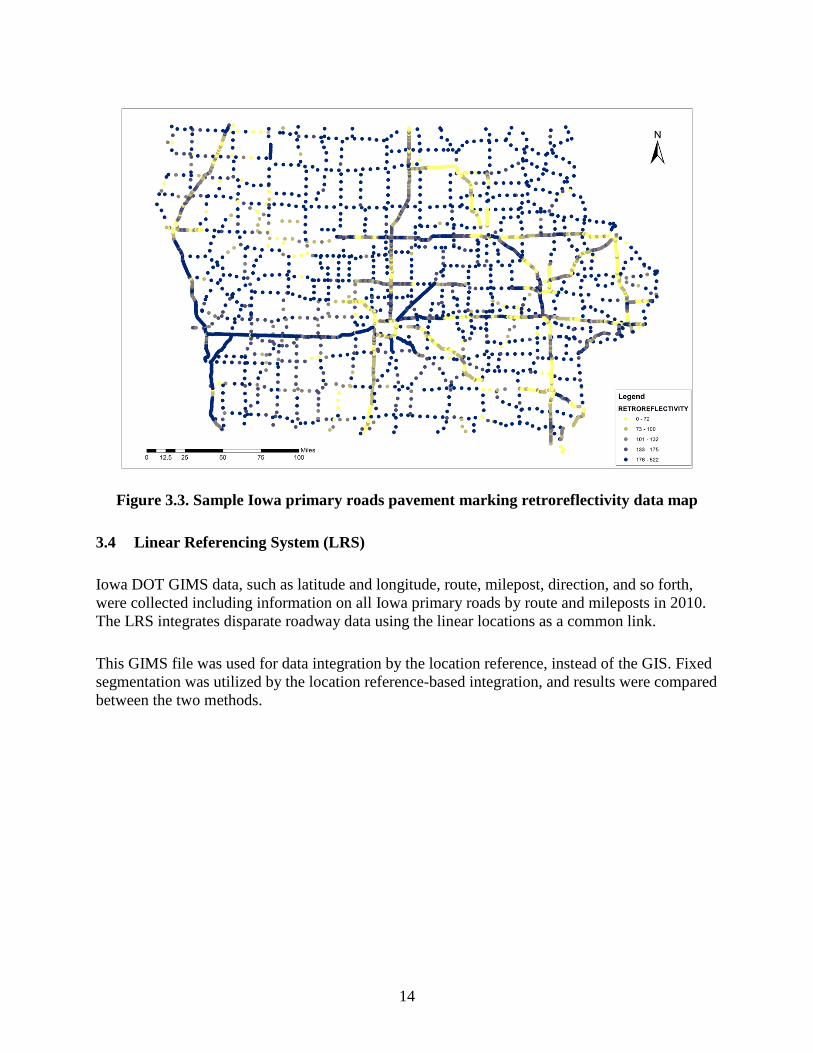
Pavement marking retroreflectivity maps by season for each year were generated using GIS.
Figure 3.3 shows an example of one of these maps. A higher value indicates better pavement
marking retroreflectivity.
14
Figure 3.3. Sample Iowa primary roads pavement marking retroreflectivity data map
3.4 Linear Referencing System (LRS)
Iowa DOT GIMS data, such as latitude and longitude, route, milepost, direction, and so forth,
were collected including information on all Iowa primary roads by route and mileposts in 2010.
The LRS integrates disparate roadway data using the linear locations as a common link.
This GIMS file was used for data integration by the location reference, instead of the GIS. Fixed
segmentation was utilized by the location reference-based integration, and results were compared
between the two methods.
15
4. DATA INTEGRATION
As one of the most important processes under asset management, data integration provides
spatial relationships between agency assets, enabling agencies to prioritize maintenance needs as
well as evaluate returns on asset improvements.
Two data integration methodologies were undertaken for this study: pure GIS-based integration
and route milepost-based integration. The GIS-based method used the spatial integration and
joining method, while the route milepost-based method applied the location-referencing method
(LRM) to integrate assets by highway location and segments.
4.1 Data Integration Concepts in Asset Management
4.1.1 Data Integration and AM
Data integration is defined as the “process of combining or linking two or more data sets from
different sources to facilitate data sharing, promote effective data gathering and analysis, and
support overall information management activities in an organization” (FHWA, Data Integration
Primer 2010).
System-level transportation decision-making, which is a primary goal of AM, requires different
levels of asset data as inputs. With these inputs, data integration provides the spatial relationship
between assets. In addition, data integration supports comprehensive decision-making processes,
with quick and convenient access to data, as well as further economic analysis.
The data integration process includes the following: 1) requirement analysis, 2) data and process
modeling, 3) alternatives, definition, evaluation, and selection, 4) database design and
specification, and 5) development, testing, and implementation (FHWA 2010).
Requirement analysis consists of business processes, such as handling data problems; user
requirements, such as purpose and uses of data; character of agency and its skills and staff
capabilities; data characteristics, such as data collection method and data type; and information
system infrastructure, such as hardware or software requirements.
After analyzing data requirements, process modeling represents the datasets and their
relationships graphically. In addition, process modeling may estimate a flow diagram, helping to
determine the design specification.
With the design flow diagram or dataset relationships, alternatives of database type should be
listed, evaluated, and selected. Common database types include fused database (single server)
and interoperable database (numerous databases with computer network links).
16
Once the database type is determined, the next step is database design. This process is comprised
of data model selection (structure and configuration of the database), data standards
identification, data reference system selection, metadata and dictionary estimation, computer
communication, etc. (FHWA, Data Integration Primer 2010).
The database design phase is followed by prototype development, testing or evaluation of the
data models or interface, and, finally, implementation of the integrated data.
4.1.2 Common Methods of Integrating
Currently, the most commonly used data integration tools or techniques include dynamic
segmentation, geo-coding/LRS, and structured query language (SQL) relationships. Geo-coding
and SQL are commonly-used tools for data integration.
Dynamic segmentation is the process of computing the spatial locations or segments of events
for highway assets stored and managed in an attribute table using a linear referencing
measurement system. Dynamic segmentation allows integration of multiple data events, data
queries, and event analysis among databases and provides visualization of datasets linked to a
common LRS. Past work has argued that dynamic segmentation is the most powerful and
suitable way for integration of AM databases (Ogle, Alluri and Sarasua 2011).
Applied to AM, GIS not only facilitates data collection, processing, and display, but also
integrates asset mapping with project management and budgeting tools so that construction,
operational, and maintenance expenses can be managed and accounted for centrally. Once
established, AM systems provide a framework to allocate scarce resources efficiently and
equitably among competing objectives.
Field personnel can take detailed GIS information with them on any number of mobile devices,
locate relevant facilities quickly, and perform detailed inspections. Deficiencies identified during
inspection can generate new work orders for maintenance and repair (ESRI 2010).
Two applications of GIS for data integration related to AM systems are as follows:
The University of Northern Iowa investigated heuristic or experience-based artificial
intelligence (AI) methodologies to optimize snow removal for winter road and bridge
maintenance in Iowa. (Salim, Strauss and Emch 2002). An Iowa DOT GIS database,
which included traffic volume and roadway inventory information for all roads in the
case study area (Black Hawk County, Iowa), was obtained and integrated with the
knowledge-based expert snow removal management system created by the researchers.
GIS was used in Pierce County, Washington to integrate information and build an AM
system on 190 traffic signals, more than 1,000 street lights, 33,420 traffic signs, and
about 1,500 miles of road in the county (Butner and Lang 2009).

17
4.2 Route Milepost-Based Integration
As a second method of data integration, a fixed segmentation road reference was used and
integrated so each row of the final data would represent a one-mile road segment, instead of a
crash, and models of crash number and asset condition could then be estimated for each road
segment by milepost. The following procedures were applied for each year from 2004 through
2009 and consolidated for all years.
4.2.1 Processes
Step 1: Road Reference Preparation
The first step was to extract data needed from REFERENCE_POST_2010 in the LRS dataset.
The route milepost reference that was prepared consisted of 11,955 rows, and each row
represents a milepost segment on different primary routes with a default direction of Dir.1 (North
or East). If the segment is divided by median, two rows presenting the same route and milepost
occurs, with Dir. 1=North/East and Dir. 2=South/West.
Step 2: Pavement Condition Data Integration
Pavement condition data were integrated by dynamic segmentation with each observation
indicating pavement condition values for various lengths of segments, with the lengths
represented by beginning and ending milepost.
Considering this situation, the pavement condition data were joined directly using Microsoft
Access with the designed query as a homogeneous route and direction in both datasets and
referenced mileposts as smaller or greater than ending or beginning pavement condition data
milepost, respectively.
Step 3: Pavement Marking Dataset Consolidation
Both the seasonal detected data and the repainting retroreflectivity data are available in
spreadsheet format, and both datasets are connected by the project so that a more comprehensive
asset condition dataset could be compiled.
While consolidating the data, the researchers noticed that the milepost information in the
repainting dataset coincides with the pavement condition data, in that, beginning and ending
milepost information are present for each repainted segment.
On the other hand, the seasonal retroreflectivity data used a fixed segmentation of five miles. As
a result, a similar procedure was undertaken to integrate marking retroreflectivity datasets, with
an additional query of join by the same line type (with WEL for white edge line, YEL for yellow
edge line, YCL for yellow centerline, and WDL for white dash line).
18
Step 4: Pavement Marking Retroreflectivity Data Integration
Given the pavement marking data were collected with a five-mile segmentation, the dataset was
enriched based on the assumption that each individual data value represents the retroreflectivity
value within the nearest five miles (data located +2 mileposts forward and +2 mileposts
backward). This modified dataset was then integrated with the extracted data in a manner
consistent with the other Access queries for this project.
Step 5: Sign Data Integration
The sign inventory includes two parts: sign location and sign detail. Before integrating, the two
parts were combined by the unique ID of each data row. Route and milepost information were
already included, and the integration by route milepost was accomplished directly.
Given this project focus is on the safety effect of the number of signs and sign condition,
regardless of sign direction, the sign facing direction was not considered as a criteria in
integrating these data.
Step 6: Crash Data Preparation and Integration
The original crash data from the Iowa DOT do not have milepost information available. As a
result, it was required to prepare and modify the crash data before integrating them with other
datasets.
The crash data were spatially joined with the GIMS map, again, and another GIMS file,
GIMS_MP_2010, was used.
In addition, the offset criteria of 30 meters for rural areas only and route number preparation was
conducted as before so the error could be minimized. After integrating by the same manner as
previous steps, about 140,000 rows were included in the final integrated data. However, the data
include many duplicate rows with the same information, except for crash ID, and this is because
each row is representing a comprehensive information row for a single crash.
A pivot table summary indicating pavement condition, marking retroreflectivity, and crash
number, was created and, at this point, the final integrated dataset was ready for further
modification and study.
4.2.2 Data Modification—Pavement Retroreflectivity Data Gaps Sufficiency
In the IPMMS dataset, pavement marking retroreflectivity was measured with five-mile
segmentation. Compared to other datasets, such as the pavement condition dataset, which has a
dynamic segmentation with the segment lengths within the rage of 0.5 to 1.5 miles, the pavement
marking retroreflectivity dataset has a relatively long segmentation.
19
In this case, with the data integration result produced by milepost, every five miles has a single
retroreflectivity data value. This situation could result in a potential inaccuracy or error for the
study. Thus, an assumption was made that every retroreflectivity reading represents an average
marking retroreflectivity within the nearest five miles, with 2.5 miles in front of the segment and
2.5 miles further from the segment for the same route index and direction.
With the assumption, a pavement retroreflectivity data gap sufficiency procedure was developed,
and the result of the fulfilled dataset was expected to produce more accurate results and better-
developed relationship estimation between asset condition and safety performance.
4.3 Summary
In the field of transportation engineering, large amounts of data are generated from management
systems, such as an AM system. Datasets come in different formats, resulting in the need for
innovative techniques in terms of managing, editing, plotting, integrating, and analyzing these
data.
In this study, datasets were integrated focusing on both crashes and roadway segments and
results indicated that the route milepost-based integration is a more applicable method,
considering the integrated data characteristics.
20
5. ESTIMATION OF ASSET CONDITION
This chapter discusses the estimation the overall asset condition of a roadway segment using a
unique index, the ACI. The ACI combines performance measurement data on pavement
condition and pavement marking retroreflectivity, such as IRI, faulting depth, friction, rutting
depth, white marking line retroreflectivity, and yellow marking line retroreflectivity. The ACI
provides a numerical rating for the condition of road segments, where 1 is poor condition, 2 is
moderate, and 3 is good.
5.1 Literature Review
Constructing an index to indicate condition given measures or performance is a widely used
method in the field of transportation engineering and, in general, civil engineering. For instance,
the U.S. Army Corps of Engineers (USACE) developed the PCI to represent the condition of a
pavement surface as a numerical index between 0 and 100.
Another study provided a step-by-step methodology to construct a US transportation
infrastructure index to help understand economic trends and promote prosperity throughout the
business sector (Oswald, et al. 2011). This transportation index provides a rich source of
historical information related to the performance of the complex and extensive transportation
infrastructure system.
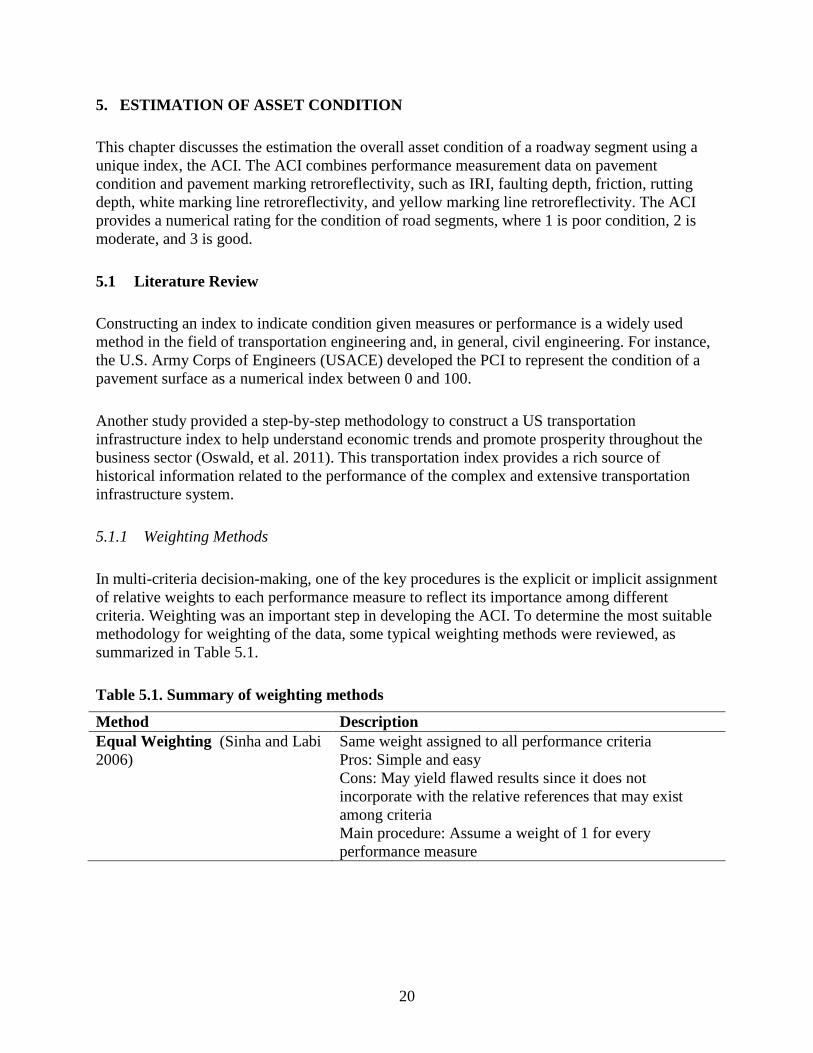
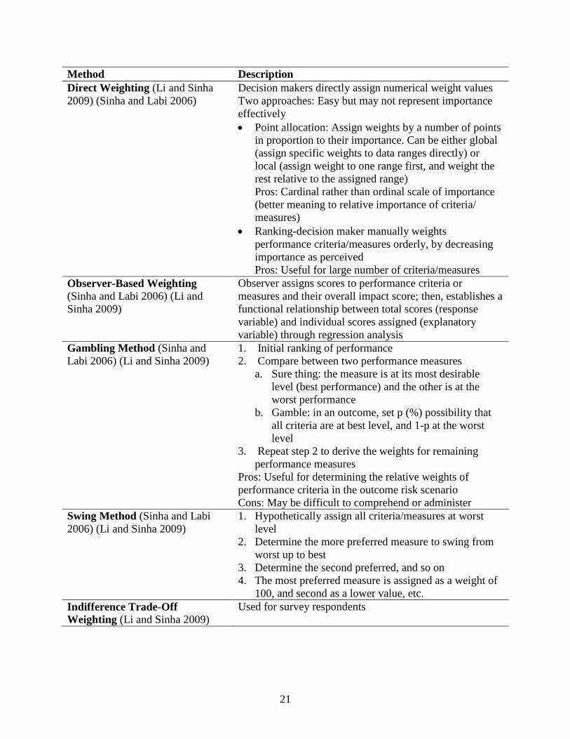
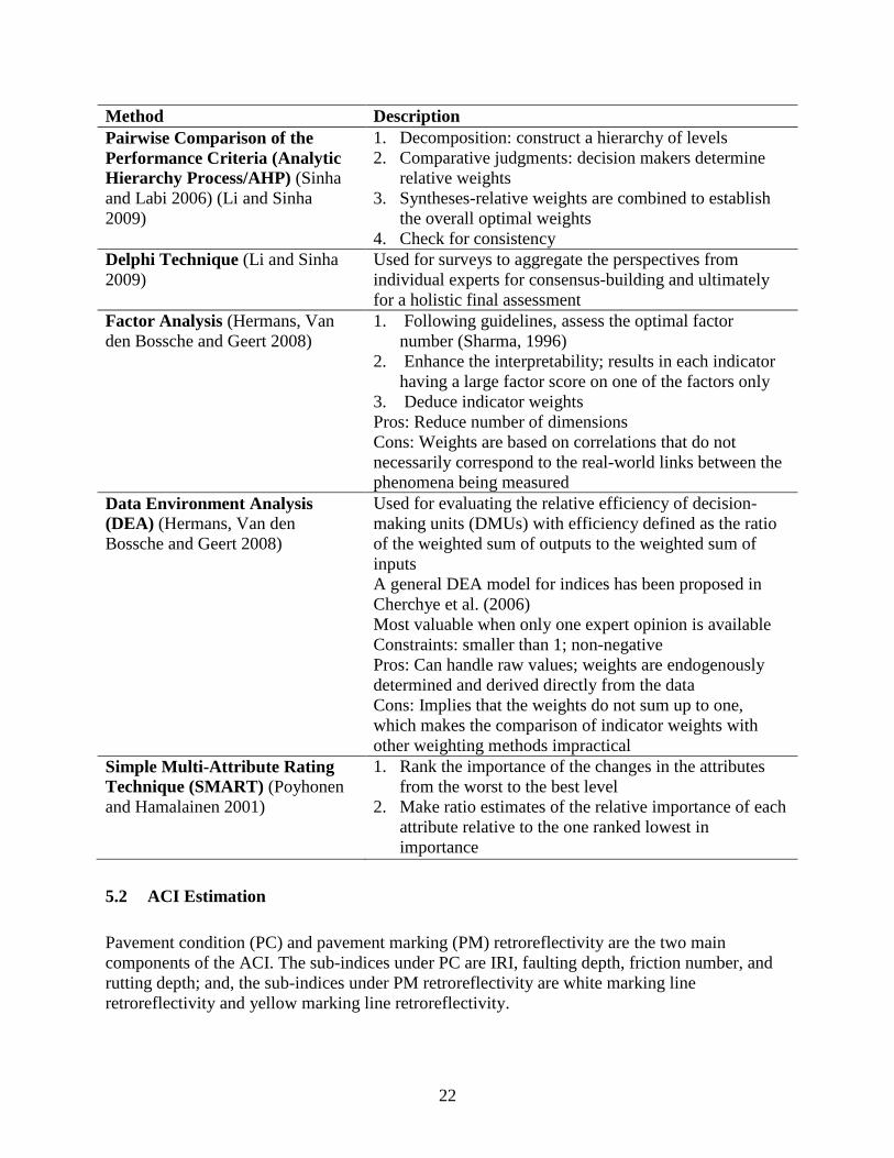
5.1.1 Weighting Methods
In multi-criteria decision-making, one of the key procedures is the explicit or implicit assignment
of relative weights to each performance measure to reflect its importance among different
criteria. Weighting was an important step in developing the ACI. To determine the most suitable
methodology for weighting of the data, some typical weighting methods were reviewed, as
summarized in Table 5.1.
Table 5.1. Summary of weighting methods
Method Description
Equal Weighting (Sinha and Labi
2006)
Same weight assigned to all performance criteria
Pros: Simple and easy
Cons: May yield flawed results since it does not
incorporate with the relative references that may exist
among criteria
Main procedure: Assume a weight of 1 for every
performance measure
21
Method Description
Direct Weighting (Li and Sinha
2009) (Sinha and Labi 2006)
Decision makers directly assign numerical weight values
Two approaches: Easy but may not represent importance
effectively
Point allocation: Assign weights by a number of points
in proportion to their importance. Can be either global
(assign specific weights to data ranges directly) or
local (assign weight to one range first, and weight the
rest relative to the assigned range)
Pros: Cardinal rather than ordinal scale of importance
(better meaning to relative importance of criteria/
measures)
Ranking-decision maker manually weights
performance criteria/measures orderly, by decreasing
importance as perceived
Pros: Useful for large number of criteria/measures
Observer-Based Weighting (Sinha and Labi 2006) (Li and
Sinha 2009)
Observer assigns scores to performance criteria or
measures and their overall impact score; then, establishes a
functional relationship between total scores (response
variable) and individual scores assigned (explanatory
variable) through regression analysis
Gambling Method (Sinha and
Labi 2006) (Li and Sinha 2009)
1. Initial ranking of performance
2. Compare between two performance measures
a. Sure thing: the measure is at its most desirable
level (best performance) and the other is at the
worst performance
b. Gamble: in an outcome, set p (%) possibility that
all criteria are at best level, and 1-p at the worst
level
3. Repeat step 2 to derive the weights for remaining
performance measures
Pros: Useful for determining the relative weights of
performance criteria in the outcome risk scenario
Cons: May be difficult to comprehend or administer
Swing Method (Sinha and Labi
2006) (Li and Sinha 2009)
1. Hypothetically assign all criteria/measures at worst
level
2. Determine the more preferred measure to swing from
worst up to best
3. Determine the second preferred, and so on
4. The most preferred measure is assigned as a weight of
100, and second as a lower value, etc.
Indifference Trade-Off
Weighting (Li and Sinha 2009)
Used for survey respondents
22
Method Description
Pairwise Comparison of the
Performance Criteria (Analytic
Hierarchy Process/AHP) (Sinha
and Labi 2006) (Li and Sinha
2009)
1. Decomposition: construct a hierarchy of levels
2. Comparative judgments: decision makers determine
relative weights
3. Syntheses-relative weights are combined to establish
the overall optimal weights
4. Check for consistency
Delphi Technique (Li and Sinha
2009)
Used for surveys to aggregate the perspectives from
individual experts for consensus-building and ultimately
for a holistic final assessment
Factor Analysis (Hermans, Van
den Bossche and Geert 2008)
1. Following guidelines, assess the optimal factor
number (Sharma, 1996)
2. Enhance the interpretability; results in each indicator
having a large factor score on one of the factors only
3. Deduce indicator weights
Pros: Reduce number of dimensions
Cons: Weights are based on correlations that do not
necessarily correspond to the real-world links between the
phenomena being measured
Data Environment Analysis
(DEA) (Hermans, Van den
Bossche and Geert 2008)
Used for evaluating the relative efficiency of decision-
making units (DMUs) with efficiency defined as the ratio
of the weighted sum of outputs to the weighted sum of
inputs
A general DEA model for indices has been proposed in
Cherchye et al. (2006)
Most valuable when only one expert opinion is available
Constraints: smaller than 1; non-negative
Pros: Can handle raw values; weights are endogenously
determined and derived directly from the data
Cons: Implies that the weights do not sum up to one,
which makes the comparison of indicator weights with
other weighting methods impractical
Simple Multi-Attribute Rating
Technique (SMART) (Poyhonen
and Hamalainen 2001)
1. Rank the importance of the changes in the attributes
from the worst to the best level
2. Make ratio estimates of the relative importance of each
attribute relative to the one ranked lowest in
importance
5.2 ACI Estimation
Pavement condition (PC) and pavement marking (PM) retroreflectivity are the two main
components of the ACI. The sub-indices under PC are IRI, faulting depth, friction number, and
rutting depth; and, the sub-indices under PM retroreflectivity are white marking line
retroreflectivity and yellow marking line retroreflectivity.
23
The white marking line retroreflectivity is the average of retroreflectivity of the white edge line
(WEL) and white dash line (WDL) in the road segment. Both of these line types are applied for
dividing traffic in the same direction. On the other hand, the yellow marking line retroreflectivity
sub-index includes the yellow edge line (YEL) and yellow centerline (YCL) on undivided
roadways and divided roadways, respectively. Both are utilized for dividing traffic in different
directions.
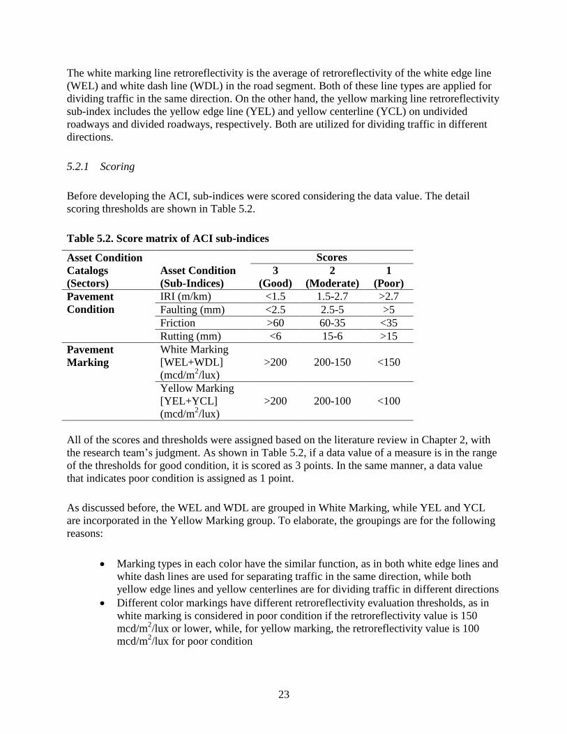
5.2.1 Scoring
Before developing the ACI, sub-indices were scored considering the data value. The detail
scoring thresholds are shown in Table 5.2.
Table 5.2. Score matrix of ACI sub-indices
Asset Condition
Catalogs
(Sectors)
Asset Condition
(Sub-Indices)
Scores
3
(Good)
2
(Moderate)
1
(Poor)
Pavement
Condition
IRI (m/km) <1.5 1.5-2.7 >2.7
Faulting (mm) <2.5 2.5-5 >5
Friction >60 60-35 <35
Rutting (mm) <6 15-6 >15
Pavement
Marking
White Marking
[WEL+WDL]
(mcd/m2/lux)
>200 200-150 <150
Yellow Marking
[YEL+YCL]
(mcd/m2/lux)
>200 200-100 <100
All of the scores and thresholds were assigned based on the literature review in Chapter 2, with
the research team’s judgment. As shown in Table 5.2, if a data value of a measure is in the range
of the thresholds for good condition, it is scored as 3 points. In the same manner, a data value
that indicates poor condition is assigned as 1 point.
As discussed before, the WEL and WDL are grouped in White Marking, while YEL and YCL
are incorporated in the Yellow Marking group. To elaborate, the groupings are for the following
reasons:
Marking types in each color have the similar function, as in both white edge lines and
white dash lines are used for separating traffic in the same direction, while both
yellow edge lines and yellow centerlines are for dividing traffic in different directions
Different color markings have different retroreflectivity evaluation thresholds, as in
white marking is considered in poor condition if the retroreflectivity value is 150
mcd/m2/lux or lower, while, for yellow marking, the retroreflectivity value is 100
mcd/m2/lux for poor condition
24
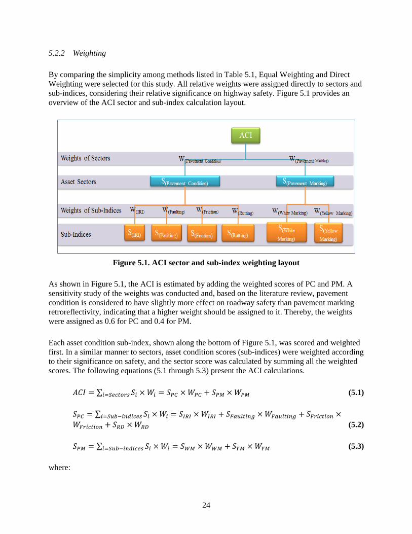
5.2.2 Weighting
By comparing the simplicity among methods listed in Table 5.1, Equal Weighting and Direct
Weighting were selected for this study. All relative weights were assigned directly to sectors and
sub-indices, considering their relative significance on highway safety. Figure 5.1 provides an
overview of the ACI sector and sub-index calculation layout.
Figure 5.1. ACI sector and sub-index weighting layout
As shown in Figure 5.1, the ACI is estimated by adding the weighted scores of PC and PM. A
sensitivity study of the weights was conducted and, based on the literature review, pavement
condition is considered to have slightly more effect on roadway safety than pavement marking
retroreflectivity, indicating that a higher weight should be assigned to it. Thereby, the weights
were assigned as 0.6 for PC and 0.4 for PM.
Each asset condition sub-index, shown along the bottom of Figure 5.1, was scored and weighted
first. In a similar manner to sectors, asset condition scores (sub-indices) were weighted according
to their significance on safety, and the sector score was calculated by summing all the weighted
scores. The following equations (5.1 through 5.3) present the ACI calculations.
∑ (5.1)
∑
(5.2)
∑ (5.3)
where:
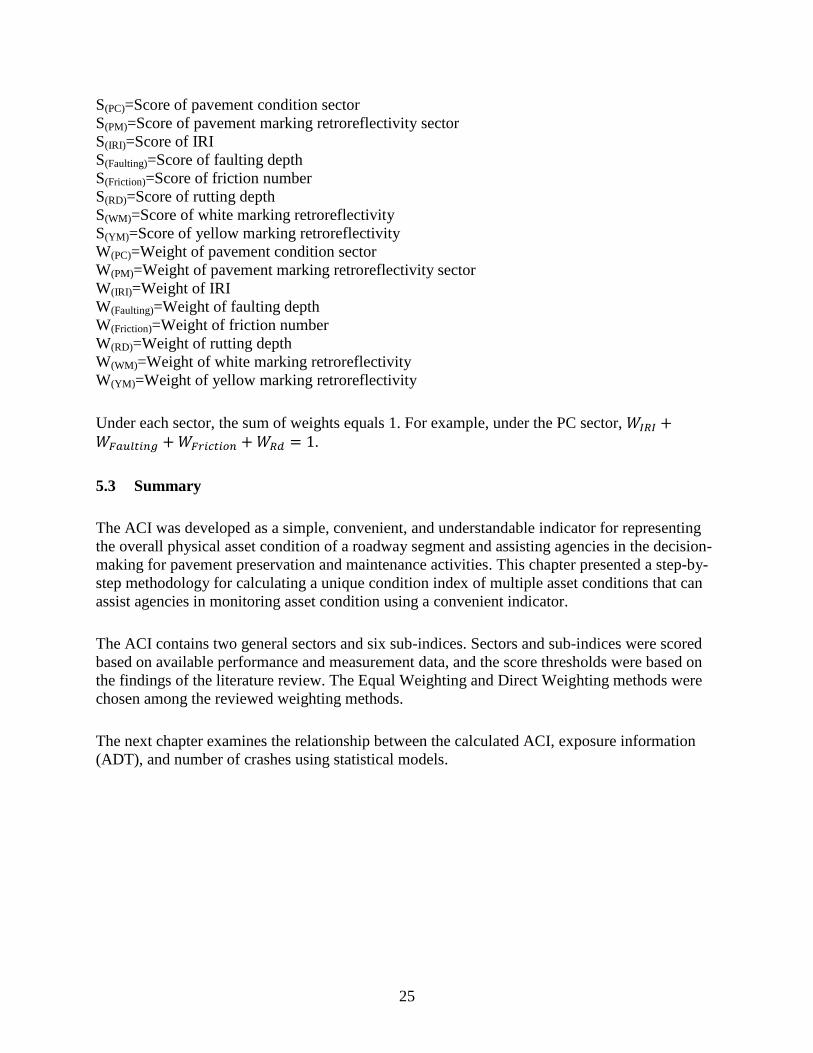
25
S(PC)=Score of pavement condition sector
S(PM)=Score of pavement marking retroreflectivity sector
S(IRI)=Score of IRI
S(Faulting)=Score of faulting depth
S(Friction)=Score of friction number
S(RD)=Score of rutting depth
S(WM)=Score of white marking retroreflectivity
S(YM)=Score of yellow marking retroreflectivity
W(PC)=Weight of pavement condition sector
W(PM)=Weight of pavement marking retroreflectivity sector
W(IRI)=Weight of IRI
W(Faulting)=Weight of faulting depth
W(Friction)=Weight of friction number
W(RD)=Weight of rutting depth
W(WM)=Weight of white marking retroreflectivity
W(YM)=Weight of yellow marking retroreflectivity
Under each sector, the sum of weights equals 1. For example, under the PC sector, .
5.3 Summary
The ACI was developed as a simple, convenient, and understandable indicator for representing
the overall physical asset condition of a roadway segment and assisting agencies in the decision-
making for pavement preservation and maintenance activities. This chapter presented a step-by-
step methodology for calculating a unique condition index of multiple asset conditions that can
assist agencies in monitoring asset condition using a convenient indicator.
The ACI contains two general sectors and six sub-indices. Sectors and sub-indices were scored
based on available performance and measurement data, and the score thresholds were based on
the findings of the literature review. The Equal Weighting and Direct Weighting methods were
chosen among the reviewed weighting methods.
The next chapter examines the relationship between the calculated ACI, exposure information
(ADT), and number of crashes using statistical models.
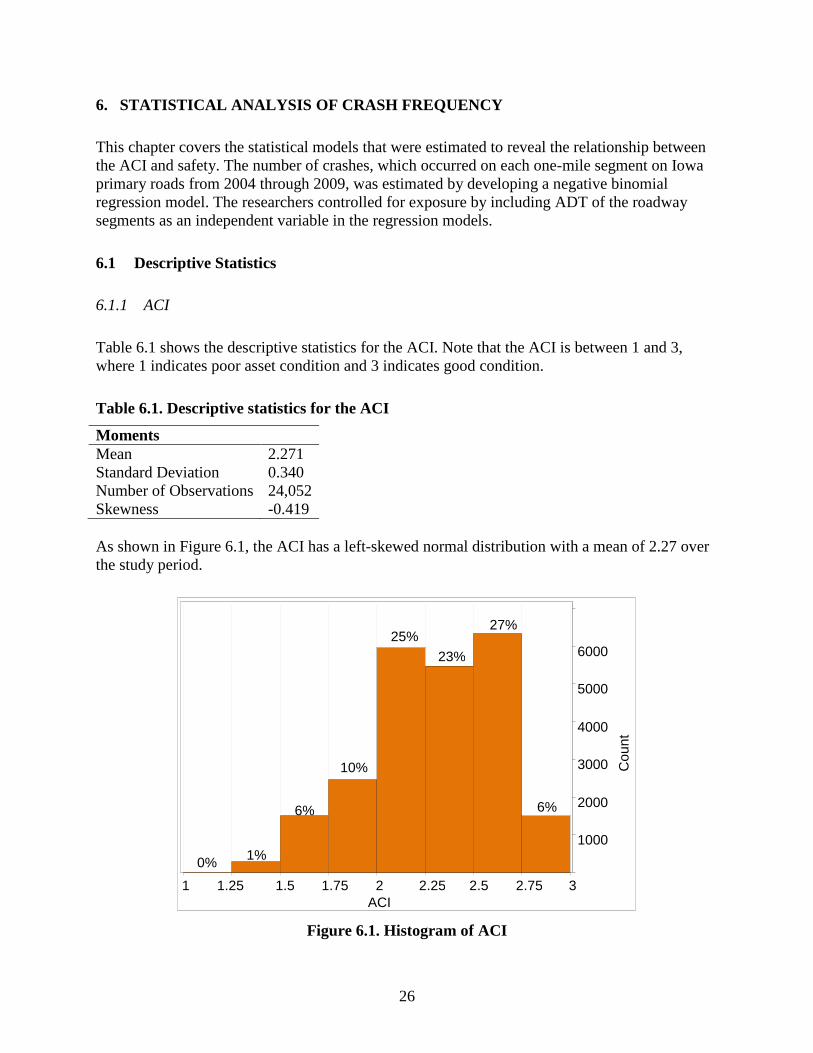
26
6. STATISTICAL ANALYSIS OF CRASH FREQUENCY
This chapter covers the statistical models that were estimated to reveal the relationship between
the ACI and safety. The number of crashes, which occurred on each one-mile segment on Iowa
primary roads from 2004 through 2009, was estimated by developing a negative binomial
regression model. The researchers controlled for exposure by including ADT of the roadway
segments as an independent variable in the regression models.
6.1 Descriptive Statistics
6.1.1 ACI
Table 6.1 shows the descriptive statistics for the ACI. Note that the ACI is between 1 and 3,
where 1 indicates poor asset condition and 3 indicates good condition.
Table 6.1. Descriptive statistics for the ACI
Moments
Mean 2.271
Standard Deviation 0.340
Number of Observations 24,052
Skewness -0.419
As shown in Figure 6.1, the ACI has a left-skewed normal distribution with a mean of 2.27 over
the study period.
Figure 6.1. Histogram of ACI
0% 1%
6%
10%
25%
23%
27%
6%
1000
2000
3000
4000
5000
6000
Co
un
t
1 1.25 1.5 1.75 2 2.25 2.5 2.75 3 ACI

27
Figure 6.2 shows the mean ACI for 2004 through 2009. The mean ACI for all six study years
was above 2.0, which represents an overall good condition.
Figure 6.2. Distribution of ACI by year
6.1.2 ADT
Table 6.2 shows the descriptive statistics for ADT.
Table 6.2. Descriptive statistics for ADT
Moments
Mean 5,758.471
Standard Deviation 8,656.995
Number of Observations 24,052
Skewness 4.287883
The ADT data follows a right-skewed normal distribution as shown in Figure 6.3.
0
1
2
3 M
ea
n (
AC
I)
2.25 2.41
2.31
2.35
2.10
2.33
2004 2005 2006 2007 2008 2009
Year

28
Figure 6.3. Histogram of ADT
As shown in Table 6.2, ADT has a large variance. As such, the natural logarithm of the ADT or
Log(ADT), was calculated and used in the models.
6.1.3 Log(ADT)
The descriptive analysis for Log(ADT) is presented in this section. The purpose of converting
ADT into Log(ADT) is to change the order of magnitude of ADT so the orders of magnitude of
all factors are close enough for estimating a statistic model rationally.
Table 6.3. Descriptive statistics of Log(ADT)
Moments
Mean 8.069
Standard Deviation 1.003
Number of Observations 24,052
Skewness 0.608
As shown in Table 6.3, the mean of Log(ADT) is about 8.1. The standard deviation (1) is also
much smaller than the standard deviation of ADT (8,657), which indicates that the Log(ADT) is
much more concentrated around the mean.
The Log(ADT) follows a right-skewed normal distribution, as shown in Figure 6.4, and the
skewness is 0.608.
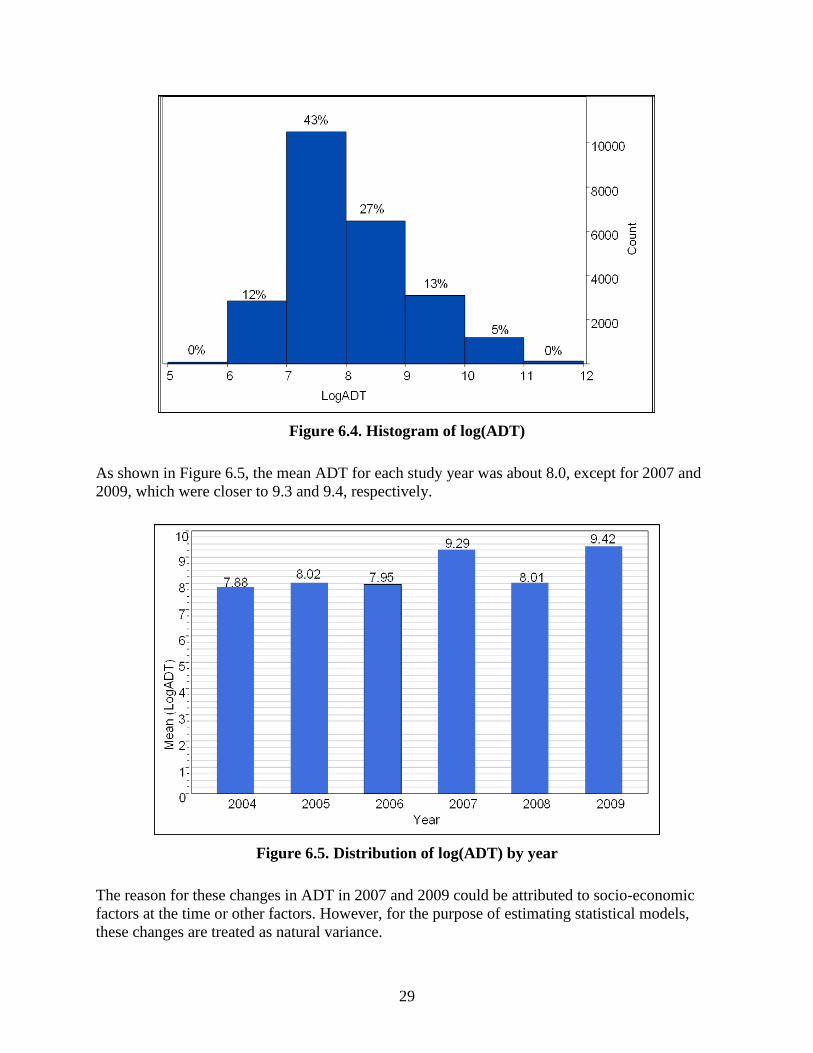
29
Figure 6.4. Histogram of log(ADT)
As shown in Figure 6.5, the mean ADT for each study year was about 8.0, except for 2007 and
2009, which were closer to 9.3 and 9.4, respectively.
Figure 6.5. Distribution of log(ADT) by year
The reason for these changes in ADT in 2007 and 2009 could be attributed to socio-economic
factors at the time or other factors. However, for the purpose of estimating statistical models,
these changes are treated as natural variance.
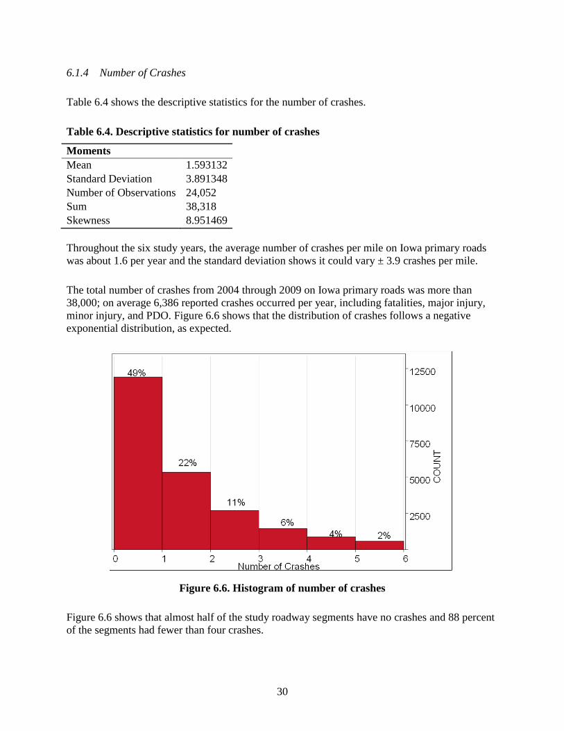
30
6.1.4 Number of Crashes
Table 6.4 shows the descriptive statistics for the number of crashes.
Table 6.4. Descriptive statistics for number of crashes
Moments
Mean 1.593132
Standard Deviation 3.891348
Number of Observations 24,052
Sum 38,318
Skewness 8.951469
Throughout the six study years, the average number of crashes per mile on Iowa primary roads
was about 1.6 per year and the standard deviation shows it could vary ± 3.9 crashes per mile.
The total number of crashes from 2004 through 2009 on Iowa primary roads was more than
38,000; on average 6,386 reported crashes occurred per year, including fatalities, major injury,
minor injury, and PDO. Figure 6.6 shows that the distribution of crashes follows a negative
exponential distribution, as expected.
Figure 6.6. Histogram of number of crashes
Figure 6.6 shows that almost half of the study roadway segments have no crashes and 88 percent
of the segments had fewer than four crashes.
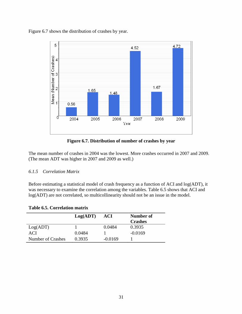
31
Figure 6.7 shows the distribution of crashes by year.
Figure 6.7. Distribution of number of crashes by year
The mean number of crashes in 2004 was the lowest. More crashes occurred in 2007 and 2009.
(The mean ADT was higher in 2007 and 2009 as well.)
6.1.5 Correlation Matrix
Before estimating a statistical model of crash frequency as a function of ACI and log(ADT), it
was necessary to examine the correlation among the variables. Table 6.5 shows that ACI and
log(ADT) are not correlated, so multicollinearity should not be an issue in the model.
Table 6.5. Correlation matrix
Log(ADT) ACI Number of
Crashes
Log(ADT) 1 0.0484 0.3935
ACI 0.0484 1 -0.0169
Number of Crashes 0.3935 -0.0169 1
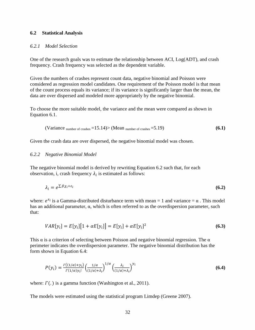
32
6.2 Statistical Analysis
6.2.1 Model Selection
One of the research goals was to estimate the relationship between ACI, Log(ADT), and crash
frequency. Crash frequency was selected as the dependent variable.
Given the numbers of crashes represent count data, negative binomial and Poisson were
considered as regression model candidates. One requirement of the Poisson model is that mean
of the count process equals its variance; if its variance is significantly larger than the mean, the
data are over dispersed and modeled more appropriately by the negative binomial.
To choose the more suitable model, the variance and the mean were compared as shown in
Equation 6.1.
(Variance number of crashes =15.14)> (Mean number of crashes =5.19) (6.1)
Given the crash data are over dispersed, the negative binomial model was chosen.
6.2.2 Negative Binomial Model
The negative binomial model is derived by rewriting Equation 6.2 such that, for each
observation, i, crash frequency is estimated as follows:
∑ (6.2)
where: is a Gamma-distributed disturbance term with mean = 1 and variance = α . This model
has an additional parameter, α, which is often referred to as the overdispersion parameter, such
that:
[ ] [ ][ [ ]] [ ] [ ] (6.3)
This α is a criterion of selecting between Poisson and negative binomial regression. The α
perimeter indicates the overdispersion parameter. The negative binomial distribution has the
form shown in Equation 6.4:
( ) (( ) )
( ) (
( ) )
(
( ) )
(6.4)
where: ( ) is a gamma function (Washington et al., 2011).
The models were estimated using the statistical program Limdep (Greene 2007).
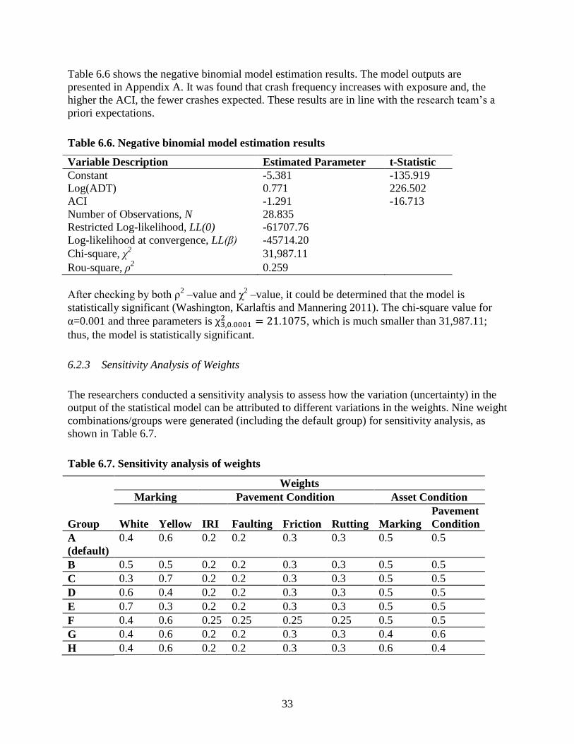
33
Table 6.6 shows the negative binomial model estimation results. The model outputs are
presented in Appendix A. It was found that crash frequency increases with exposure and, the
higher the ACI, the fewer crashes expected. These results are in line with the research team’s a
priori expectations.
Table 6.6. Negative binomial model estimation results
Variable Description Estimated Parameter t-Statistic
Constant -5.381 -135.919
Log(ADT) 0.771 226.502
ACI -1.291 -16.713
Number of Observations, N 28.835
Restricted Log-likelihood, LL(0) -61707.76
Log-likelihood at convergence, LL(β) -45714.20
Chi-square, χ2 31,987.11
Rou-square, ρ2 0.259
After checking by both ρ2 –value and χ
2 –value, it could be determined that the model is
statistically significant (Washington, Karlaftis and Mannering 2011). The chi-square value for
α=0.001 and three parameters is , which is much smaller than 31,987.11;
thus, the model is statistically significant.
6.2.3 Sensitivity Analysis of Weights
The researchers conducted a sensitivity analysis to assess how the variation (uncertainty) in the
output of the statistical model can be attributed to different variations in the weights. Nine weight
combinations/groups were generated (including the default group) for sensitivity analysis, as
shown in Table 6.7.
Table 6.7. Sensitivity analysis of weights
Group
Weights
Marking Pavement Condition Asset Condition
White Yellow IRI Faulting Friction Rutting Marking
Pavement
Condition
A
(default)
0.4 0.6 0.2 0.2 0.3 0.3 0.5 0.5
B 0.5 0.5 0.2 0.2 0.3 0.3 0.5 0.5
C 0.3 0.7 0.2 0.2 0.3 0.3 0.5 0.5
D 0.6 0.4 0.2 0.2 0.3 0.3 0.5 0.5
E 0.7 0.3 0.2 0.2 0.3 0.3 0.5 0.5
F 0.4 0.6 0.25 0.25 0.25 0.25 0.5 0.5
G 0.4 0.6 0.2 0.2 0.3 0.3 0.4 0.6
H 0.4 0.6 0.2 0.2 0.3 0.3 0.6 0.4
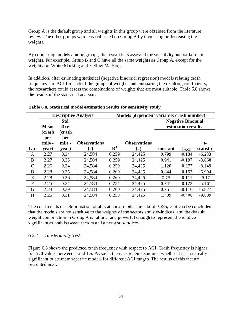
34
Group A is the default group and all weights in this group were obtained from the literature
review. The other groups were created based on Group A by increasing or decreasing the
weights.
By comparing models among groups, the researchers assessed the sensitivity and variation of
weights. For example, Group B and C have all the same weights as Group A, except for the
weights for White Marking and Yellow Marking.
In addition, after estimating statistical (negative binomial regression) models relating crash
frequency and ACI for each of the groups of weights and comparing the resulting coefficients,
the researchers could assess the combinations of weights that are most suitable. Table 6.8 shows
the results of the statistical analysis.
Table 6.8. Statistical model estimation results for sensitivity study
Gp.
Descriptive Analysis Models (dependent variable: crash number)
Mean
(crash
per
mile -
year)
Std.
Dev.
(crash
per
mile -
year)
Observations
(#) R2
Observations
(#)
Negative Binomial
estimation results
constant βACI
t-
statistic
A 2.27 0.34 24,584 0.259 24,425 0.799 -0.134 -6.233
B 2.27 0.35 24,584 0.259 24,425 0.941 -0.197 -8.668
C 2.26 0.34 24,584 0.259 24,425 1.120 -0.277 -8.149
D 2.28 0.35 24,584 0.260 24,425 0.844 -0.153 -6.904
E 2.28 0.36 24,584 0.260 24,425 0.75 -0.111 -5.17
F 2.25 0.34 24,584 0.251 24,425 0.741 -0.123 -5.161
G 2.28 0.39 24,584 0.260 24,425 0.761 -0.116 -5.827
H 2.25 0.31 24,584 0.258 24,425 1.409 -0.408 -9.809
The coefficients of determination of all statistical models are about 0.385, so it can be concluded
that the models are not sensitive to the weights of the sectors and sub-indices, and the default
weight combination in Group A is rational and powerful enough to represent the relative
significances both between sectors and among sub-indices.
6.2.4 Transferability Test
Figure 6.8 shows the predicted crash frequency with respect to ACI. Crash frequency is higher
for ACI values between 1 and 1.5. As such, the researchers examined whether it is statistically
significant to estimate separate models for different ACI ranges. The results of this test are
presented next.
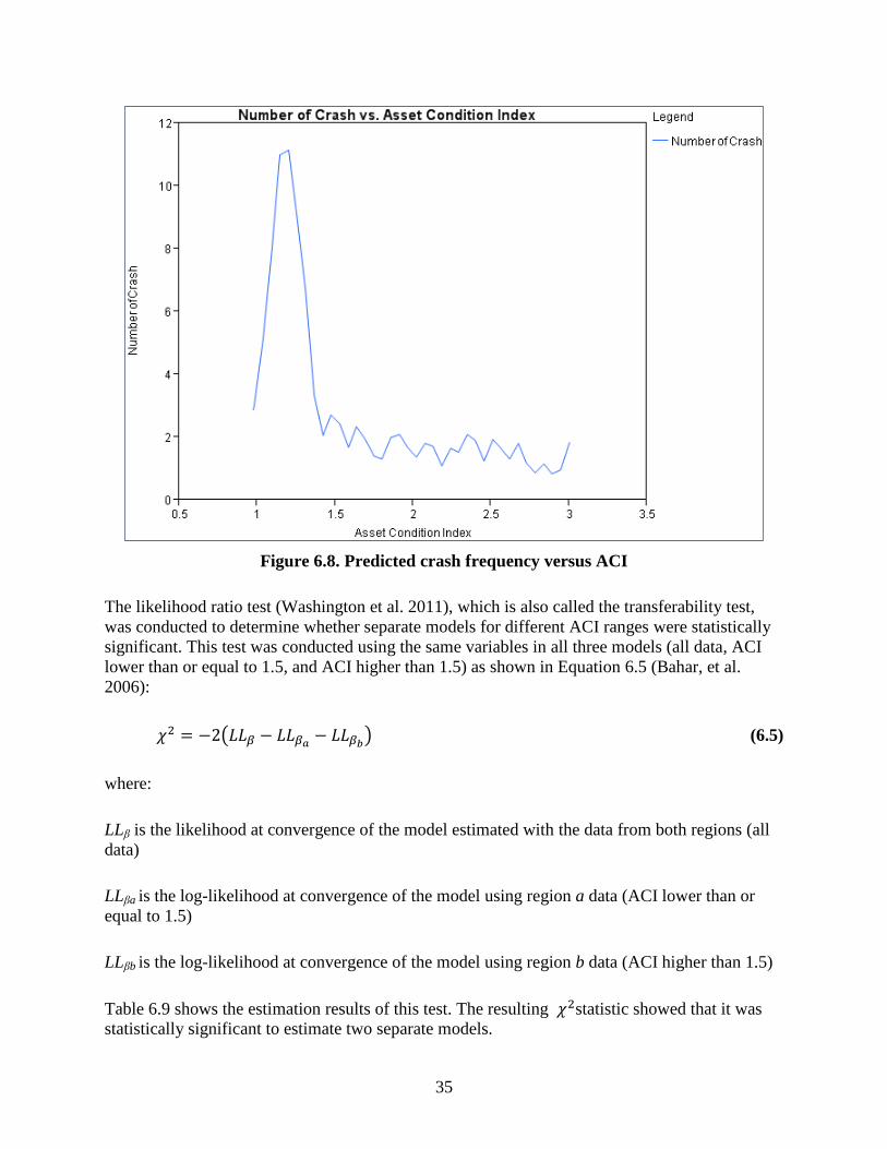
35
Figure 6.8. Predicted crash frequency versus ACI
The likelihood ratio test (Washington et al. 2011), which is also called the transferability test,
was conducted to determine whether separate models for different ACI ranges were statistically
significant. This test was conducted using the same variables in all three models (all data, ACI
lower than or equal to 1.5, and ACI higher than 1.5) as shown in Equation 6.5 (Bahar, et al.
2006):
( ) (6.5)
where:
LLβ is the likelihood at convergence of the model estimated with the data from both regions (all
data)
LLβa is the log-likelihood at convergence of the model using region a data (ACI lower than or
equal to 1.5)
LLβb is the log-likelihood at convergence of the model using region b data (ACI higher than 1.5)
Table 6.9 shows the estimation results of this test. The resulting statistic showed that it was
statistically significant to estimate two separate models.
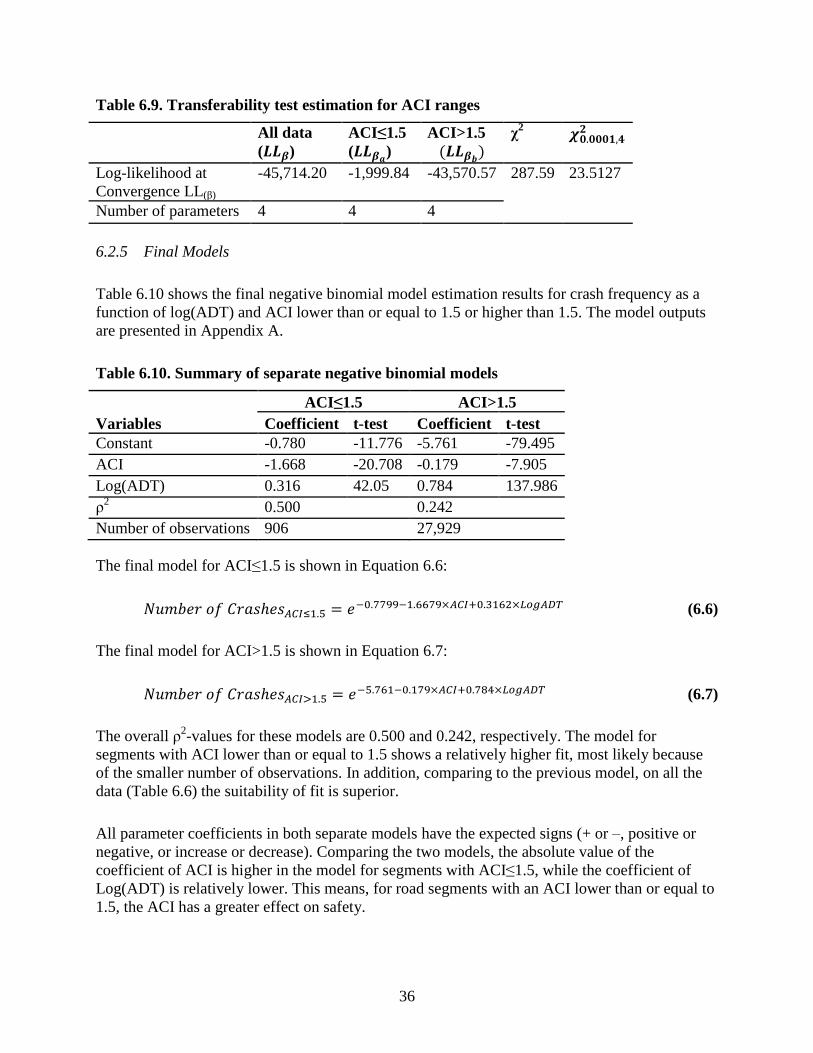
36
Table 6.9. Transferability test estimation for ACI ranges
All data
( )
ACI≤1.5
( ) ACI>1.5
( ) χ
2
Log-likelihood at
Convergence LL(β)
-45,714.20 -1,999.84 -43,570.57 287.59 23.5127
Number of parameters 4 4 4
6.2.5 Final Models
Table 6.10 shows the final negative binomial model estimation results for crash frequency as a
function of log(ADT) and ACI lower than or equal to 1.5 or higher than 1.5. The model outputs
are presented in Appendix A.
Table 6.10. Summary of separate negative binomial models
Variables
ACI≤1.5 ACI>1.5
Coefficient t-test Coefficient t-test
Constant -0.780 -11.776 -5.761 -79.495
ACI -1.668 -20.708 -0.179 -7.905
Log(ADT) 0.316 42.05 0.784 137.986
ρ2 0.500 0.242
Number of observations 906 27,929
The final model for ACI≤1.5 is shown in Equation 6.6:
(6.6)
The final model for ACI>1.5 is shown in Equation 6.7:
(6.7)
The overall ρ2-values for these models are 0.500 and 0.242, respectively. The model for
segments with ACI lower than or equal to 1.5 shows a relatively higher fit, most likely because
of the smaller number of observations. In addition, comparing to the previous model, on all the
data (Table 6.6) the suitability of fit is superior.
All parameter coefficients in both separate models have the expected signs (+ or –, positive or
negative, or increase or decrease). Comparing the two models, the absolute value of the
coefficient of ACI is higher in the model for segments with ACI≤1.5, while the coefficient of
Log(ADT) is relatively lower. This means, for road segments with an ACI lower than or equal to
1.5, the ACI has a greater effect on safety.
37
6.3 Summary
The researchers used negative binomial models to predict the relationship between crash
frequency and the ACI. The estimation results indicated that the higher the ACI of a roadway
segment, the lower the number of crashes expected. In addition, the higher traffic exposure
Log(ADT) on a roadway segment, the higher the number of crashes expected.
The sensitivity analysis of weights revealed that the statistical model estimation results relating
crash frequency to ACI were not sensitive to the assumed weights of ACI sectors and sub-
indices. These results suggested that the default assumptions (based on the literature review)
could be adopted.
In addition, the transferability test showed that separate negative binomial models for different
ACI ranges better explain the relationship between crash frequency, ACI, and Log(ADT). The
researchers found that the effect of ACI on crash frequency on roadway segments with ACI
lower than or equal to 1.5 was higher and, as such, these segments should have priority for
preservation or maintenance.
38
7. EVALUATION OF ASSET TREATMENT STRATEGIES
This chapter describes the methodology used to evaluate six different pavement condition or
pavement marking improvement strategies in terms of economic efficiency and crash reduction
and the corresponding results.
The estimated results using the models presented in the last chapter were used to assess the
economic feasibility of these treatment strategies, so that agencies can utilize the information to
select projects and make better decisions.
Economic efficiency was evaluated using two methods: single-year benefit-cost ratio (BCR)
analysis and five-year net present value (NPV) analysis, one year and five years after
implementing alternative treatment strategies, respectively. Benefits represent safety
improvements in terms of crash reduction.
7.1 Goal of the Evaluation
The goal of this evaluation is to develop a method for selecting asset treatment strategies that
have an impact on both asset condition and safety in terms of crash reduction. The one-year BCR
analysis and five-year NPV analysis were adopted for different study periods in a bid to
prioritize the treatment strategies in the short and long term.
7.2 Treatment Alternatives
The researchers selected and grouped six improvement treatments into the three that would
improve pavement condition and the three that would improve pavement marking. PC treatment
improvement alternatives included pavement reconstruction, major rehabilitation, and minor
rehabilitation. The three PM material replacement types selected were regular paint, durable
material marking, and tape markings.
7.2.1 Pavement Condition Alternatives
The selection of a treatment strategy among reconstruction, major rehabilitation, and minor
rehabilitation is based on current pavement condition, target level of service, and budget
constraints.
Pavement reconstruction involves the complete removal of an existing pavement to the sub-
grade and construction of a new pavement structure. This most expensive strategy is usually
needed when the existing pavement has deteriorated to a condition that cannot be salvaged with
corrective action (MassDOT 2006). The estimated unit cost of this type of pavement treatment is
approximately $1,000,000/mile. Service life of a pavement after reconstruction is expected to be
20 years.

39
Pavement rehabilitation, which is a major activity for all highway agencies, can be defined as a
structural or functional pavement enhancement that produces a substantial extension in service
life by substantially improving pavement condition and ride quality (Hall et al., 2001).
When selecting a rehabilitation strategy, agencies select the most cost-effective rehabilitation
strategy given a set of criteria, which may include reduced service life, life-cycle cost, and
budgetary constraints. According to the current pavement condition, different rehabilitation
strategies can be selected for different types of pavement, distress types, levels of rehabilitation,
and target service life extension.
Major rehabilitation can be selected when maintenance is needed on the pavement structure,
relatively-more serious distresses are observed, or longer service life extension is expected. The
cost of this type of work is estimated as $500,000/mile and life cycle is assumed to be 10 years.
On the other hand, minor rehabilitation involves surface overlaying, repairing joints, and some
other relatively smaller maintenance operations. The cost of this type of work is approximately
$150,000/mile, and its life cycle is assumed to be three years.
7.2.2 Pavement Marking Alternatives
Three types of pavement marking materials were selected as pavement marking replacement
alternatives: regular paint, durable marking, and tape markings. These alternatives are currently
used by the Iowa DOT on different types of marking lines.
Regular paint is the most commonly used treatment among agencies. More than 95 percent of
Iowa roadways are marked using fast-drying waterborne paints. Regular paint costs relatively
less than other types of markings; however, life cycle is also typically shorter.
As mentioned in the Chapter 4, the Iowa DOT repaints pavement markings twice per year, in
spring and fall, so the service life of this type of marking is assumed to be half a year. The cost
of regular paint marking is assumed to be $1,188/mile.
Durable markings are expected to have relatively longer service lives than regular paint and, as a
result, have higher cost-effectiveness or lower life-cycle cost than regular paint. The Iowa DOT
started to evaluate and utilize durable waterborne paints with glass beads, which are considered
durable marking, in 2005.
Given the need in Iowa for snow plowing (due to winter weather), pavement markings can
deteriorate significantly. The estimated unit cost of durable marking is $11,880/mile and the
service life is assumed to be two years. (The cost of winter maintenance is not taken into account
in this unit cost.)
40
Tape marking is used typically as a transverse marking material (e.g., crosswalks, stop bars).
Tape marking performs well on both portland cement concrete (PCC) and asphalt cement
concrete (ACC) pavements (Thomas and Schloz 2001).
In general, tape marking has a high initial cost; however, tape marking is relatively easy to install
and has relatively long durability, depending on the placement location. In addition, when tape is
installed on new ACC pavement sections, the road can be open to traffic as soon as the pavement
is ready. Tape marking provides the additional advantage of avoiding the need for temporary
marking materials because it can be installed immediately after construction is complete (and not
have to wait up to two weeks for installation).
The estimated unit cost of tape marking is $47.520/mile and the service life is assumed to be five
years.
7.3 Relative ACI Improvement and Depreciation Rate
Before conducting the economic analysis, each treatment alternative was assigned a relative
improvement value on the ACI scale of 0 to 3. The relative improvement values were estimated
considering the alternative’s impact on safety in terms of reducing crash frequency, as
documented in the literature. Given that ACI is an index between 1 and 3, the improved ACI
cannot be higher than 3 regardless of initial condition.
AC depreciation is an important consideration for monitoring, performance measuring, and
pavement life-cycle cost analysis. This study considers AC depreciation and straight-line
depreciation in the five-year NPV analysis.
In the previous chapter, it was shown that roadway segments with ACI lower than or equal to 1.5
have relatively higher crash frequency. Thus, 1.5 is considered as a critical value of ACI. Based
on straight-line depreciation, the depreciation rate is calculated as shown in Equation 7.1:
(7.1)
The relative improvement values for treatment alternatives, respective costs, service lives, and
depreciation rates are shown in Table 7.1.
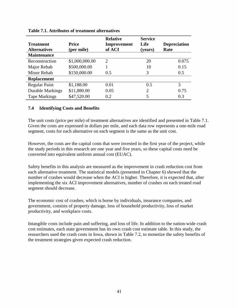
41
Table 7.1. Attributes of treatment alternatives
Treatment
Alternatives
Price
(per mile)
Relative
Improvement
of ACI
Service
Life
(years)
Depreciation
Rate
Maintenance
Reconstruction $1,000,000.00 2 20 0.075
Major Rehab $500,000.00 1 10 0.15
Minor Rehab $150,000.00 0.5 3 0.5
Replacement
Regular Paint $1,188.00 0.01 0.5 3
Durable Markings $11,880.00 0.05 2 0.75
Tape Markings $47,520.00 0.2 5 0.3
7.4 Identifying Costs and Benefits
The unit costs (price per mile) of treatment alternatives are identified and presented in Table 7.1.
Given the costs are expressed in dollars per mile, and each data row represents a one-mile road
segment, costs for each alternative on each segment is the same as the unit cost.
However, the costs are the capital costs that were invested in the first year of the project, while
the study periods in this research are one year and five years, so these capital costs need be
converted into equivalent uniform annual cost (EUAC).
Safety benefits in this analysis are measured as the improvement in crash reduction cost from
each alternative treatment. The statistical models (presented in Chapter 6) showed that the
number of crashes would decrease when the ACI is higher. Therefore, it is expected that, after
implementing the six ACI improvement alternatives, number of crashes on each treated road
segment should decrease.
The economic cost of crashes, which is borne by individuals, insurance companies, and
government, consists of property damage, loss of household productivity, loss of market
productivity, and workplace costs.
Intangible costs include pain and suffering, and loss of life. In addition to the nation-wide crash
cost estimates, each state government has its own crash cost estimate table. In this study, the
researchers used the crash costs in Iowa, shown in Table 7.2, to monetize the safety benefits of
the treatment strategies given expected crash reduction.
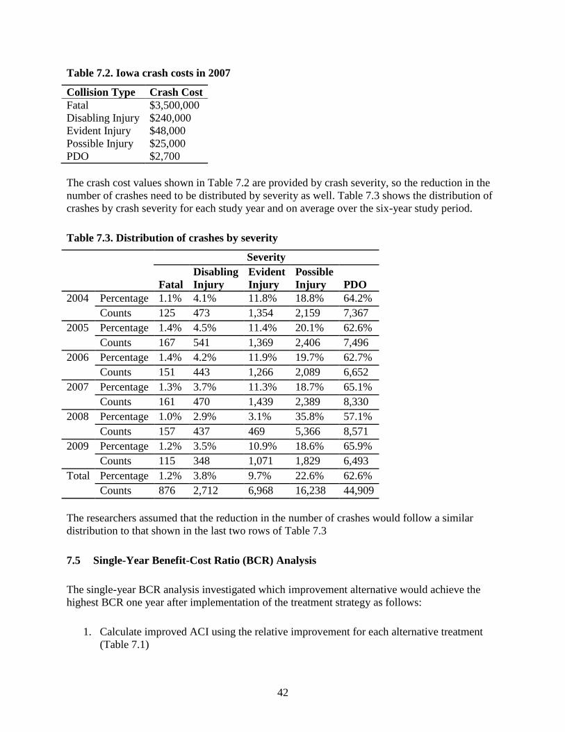
42
Table 7.2. Iowa crash costs in 2007
Collision Type Crash Cost
Fatal $3,500,000
Disabling Injury $240,000
Evident Injury $48,000
Possible Injury $25,000
PDO $2,700
The crash cost values shown in Table 7.2 are provided by crash severity, so the reduction in the
number of crashes need to be distributed by severity as well. Table 7.3 shows the distribution of
crashes by crash severity for each study year and on average over the six-year study period.
Table 7.3. Distribution of crashes by severity
Severity
Fatal
Disabling
Injury
Evident
Injury
Possible
Injury PDO
2004 Percentage 1.1% 4.1% 11.8% 18.8% 64.2%
Counts 125 473 1,354 2,159 7,367
2005 Percentage 1.4% 4.5% 11.4% 20.1% 62.6%
Counts 167 541 1,369 2,406 7,496
2006 Percentage 1.4% 4.2% 11.9% 19.7% 62.7%
Counts 151 443 1,266 2,089 6,652
2007 Percentage 1.3% 3.7% 11.3% 18.7% 65.1%
Counts 161 470 1,439 2,389 8,330
2008 Percentage 1.0% 2.9% 3.1% 35.8% 57.1%
Counts 157 437 469 5,366 8,571
2009 Percentage 1.2% 3.5% 10.9% 18.6% 65.9%
Counts 115 348 1,071 1,829 6,493
Total Percentage 1.2% 3.8% 9.7% 22.6% 62.6%
Counts 876 2,712 6,968 16,238 44,909
The researchers assumed that the reduction in the number of crashes would follow a similar
distribution to that shown in the last two rows of Table 7.3
7.5 Single-Year Benefit-Cost Ratio (BCR) Analysis
The single-year BCR analysis investigated which improvement alternative would achieve the
highest BCR one year after implementation of the treatment strategy as follows:
1. Calculate improved ACI using the relative improvement for each alternative treatment
(Table 7.1)
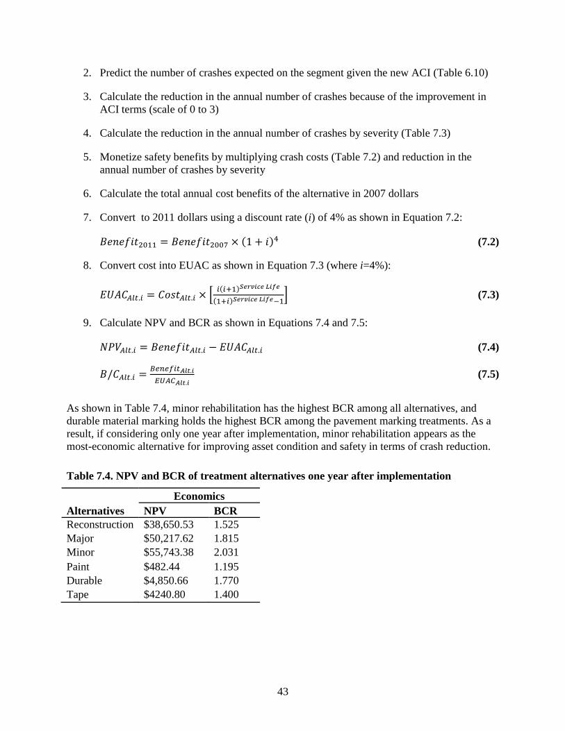
43
2. Predict the number of crashes expected on the segment given the new ACI (Table 6.10)
3. Calculate the reduction in the annual number of crashes because of the improvement in
ACI terms (scale of 0 to 3)
4. Calculate the reduction in the annual number of crashes by severity (Table 7.3)
5. Monetize safety benefits by multiplying crash costs (Table 7.2) and reduction in the
annual number of crashes by severity
6. Calculate the total annual cost benefits of the alternative in 2007 dollars
7. Convert to 2011 dollars using a discount rate (i) of 4% as shown in Equation 7.2:
( ) (7.2)
8. Convert cost into EUAC as shown in Equation 7.3 (where i=4%):
[ ( )
( ) ] (7.3)
9. Calculate NPV and BCR as shown in Equations 7.4 and 7.5:
(7.4)
(7.5)
As shown in Table 7.4, minor rehabilitation has the highest BCR among all alternatives, and
durable material marking holds the highest BCR among the pavement marking treatments. As a
result, if considering only one year after implementation, minor rehabilitation appears as the
most-economic alternative for improving asset condition and safety in terms of crash reduction.
Table 7.4. NPV and BCR of treatment alternatives one year after implementation
Alternatives
Economics
NPV BCR
Reconstruction $38,650.53 1.525
Major $50,217.62 1.815
Minor $55,743.38 2.031
Paint $482.44 1.195
Durable $4,850.66 1.770
Tape $4240.80 1.400
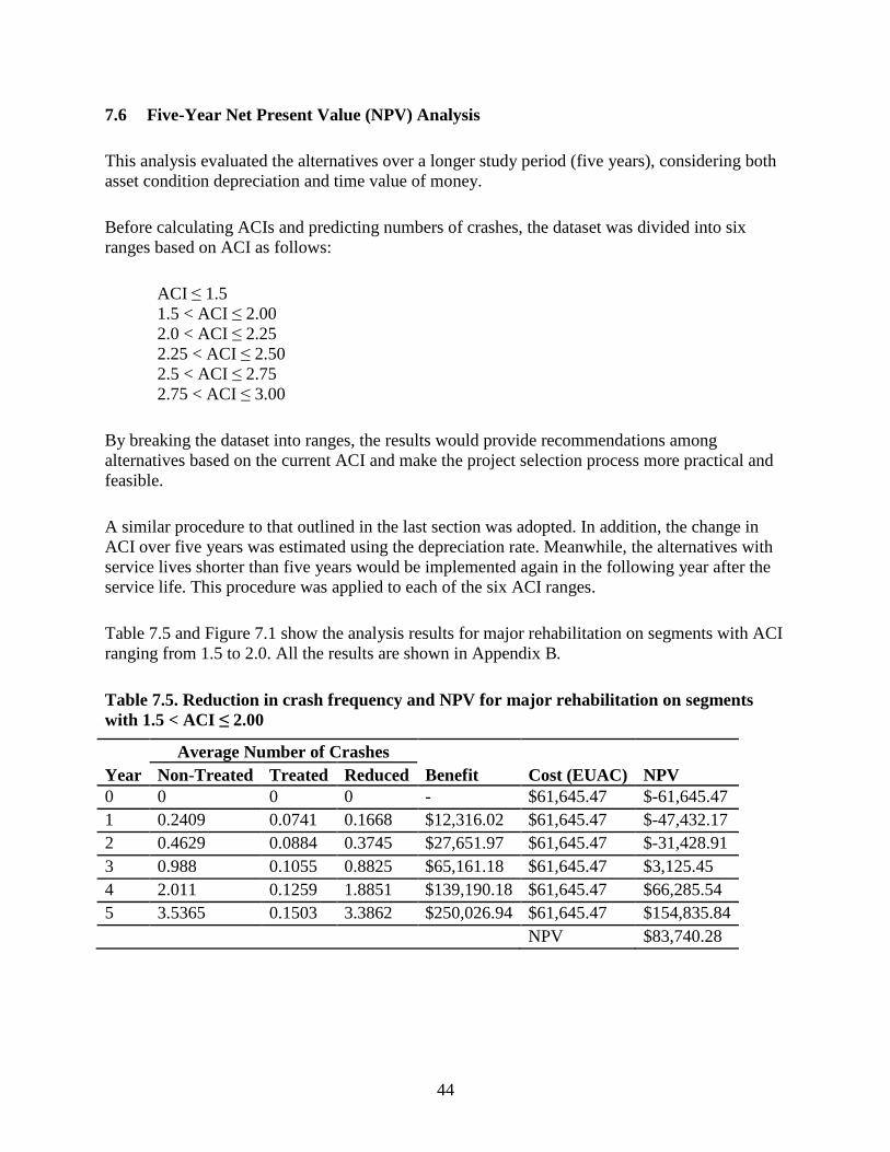
44
7.6 Five-Year Net Present Value (NPV) Analysis
This analysis evaluated the alternatives over a longer study period (five years), considering both
asset condition depreciation and time value of money.
Before calculating ACIs and predicting numbers of crashes, the dataset was divided into six
ranges based on ACI as follows:
ACI ≤ 1.5
1.5 < ACI ≤ 2.00
2.0 < ACI ≤ 2.25
2.25 < ACI ≤ 2.50
2.5 < ACI ≤ 2.75
2.75 < ACI ≤ 3.00
By breaking the dataset into ranges, the results would provide recommendations among
alternatives based on the current ACI and make the project selection process more practical and
feasible.
A similar procedure to that outlined in the last section was adopted. In addition, the change in
ACI over five years was estimated using the depreciation rate. Meanwhile, the alternatives with
service lives shorter than five years would be implemented again in the following year after the
service life. This procedure was applied to each of the six ACI ranges.
Table 7.5 and Figure 7.1 show the analysis results for major rehabilitation on segments with ACI
ranging from 1.5 to 2.0. All the results are shown in Appendix B.
Table 7.5. Reduction in crash frequency and NPV for major rehabilitation on segments
with 1.5 < ACI ≤ 2.00
Year
Average Number of Crashes
Benefit Cost (EUAC) NPV Non-Treated Treated Reduced
0 0 0 0 - $61,645.47 $-61,645.47
1 0.2409 0.0741 0.1668 $12,316.02 $61,645.47 $-47,432.17
2 0.4629 0.0884 0.3745 $27,651.97 $61,645.47 $-31,428.91
3 0.988 0.1055 0.8825 $65,161.18 $61,645.47 $3,125.45
4 2.011 0.1259 1.8851 $139,190.18 $61,645.47 $66,285.54
5 3.5365 0.1503 3.3862 $250,026.94 $61,645.47 $154,835.84
NPV $83,740.28
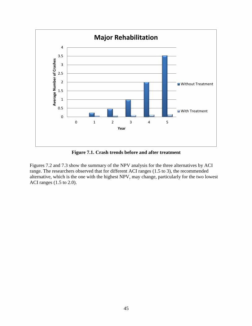
45
Figure 7.1. Crash trends before and after treatment
Figures 7.2 and 7.3 show the summary of the NPV analysis for the three alternatives by ACI
range. The researchers observed that for different ACI ranges (1.5 to 3), the recommended
alternative, which is the one with the highest NPV, may change, particularly for the two lowest
ACI ranges (1.5 to 2.0).
0
0.5
1
1.5
2
2.5
3
3.5
4
0 1 2 3 4 5
Ave
rage
Nu
mb
er
of
Cra
she
s
Year
Major Rehabilitation
Without Treatment
With Treatment
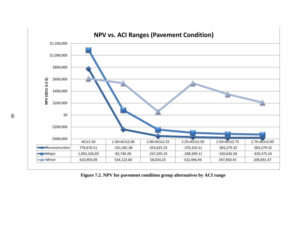
46
Figure 7.2. NPV for pavement condition group alternatives by ACI range
ACI≤1.50 1.50<ACI≤2.00 2.00<ACI≤2.25 2.25<ACI≤2.50 2.50<ACI≤2.75 2.75<ACI≤3.00
Reconstruction 776,676.51 -241,381.06 -353,625.25 -370,103.21 -383,279.32 -383,279.32
Major 1,092,326.69 83,740.28 -247,205.25 -298,399.11 -320,636.58 -329,375.24
Minor 610,903.09 534,122.00 58,034.25 532,496.94 347,850.45 209,691.47
-$400,000
-$200,000
$0
$200,000
$400,000
$600,000
$800,000
$1,000,000
$1,200,000N
PV
(2
01
1 U
.S $
)
NPV vs. ACI Ranges (Pavement Condition)
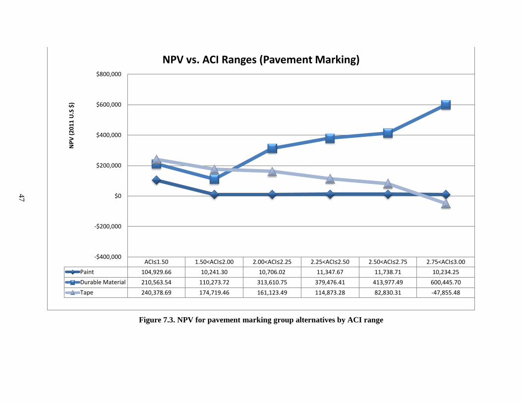
47
Figure 7.3. NPV for pavement marking group alternatives by ACI range
ACI≤1.50 1.50<ACI≤2.00 2.00<ACI≤2.25 2.25<ACI≤2.50 2.50<ACI≤2.75 2.75<ACI≤3.00
Paint 104,929.66 10,241.30 10,706.02 11,347.67 11,738.71 10,234.25
Durable Material 210,563.54 110,273.72 313,610.75 379,476.41 413,977.49 600,445.70
Tape 240,378.69 174,719.46 161,123.49 114,873.28 82,830.31 -47,855.48
-$400,000
-$200,000
$0
$200,000
$400,000
$600,000
$800,000N
PV
(2
01
1 U
.S $
)
NPV vs. ACI Ranges (Pavement Marking)
48 48
For segments with an ACI higher than 2.0, minor rehabilitation to improve pavement condition is
more cost-effective than the other strategies, while durable markings are more cost-effective than
the other treatments to improve pavement marking condition. For segments with an ACI between
1.5 and 2.0, minor rehabilitation and tape marking are recommended, while for segments with an
ACI lower or equal to 1.5, major rehabilitation and tape markings are the preferred alternatives.
7.7 Summary
In this chapter, the single-year BCR analysis and five-year NPV analysis were presented. Both
short-term and long-term safety benefits in terms of crash reduction costs and treatment costs
were estimated for six alternative treatment strategies.
Minor rehabilitation and durable marking are recommended as more cost-effective treatment
alternatives in the short-term. In the long-term, the same recommendation holds for segments
with an ACI higher than 2.0. For segments with an ACI lower than 1.5, major rehabilitation and
tape marking are highly recommended.
49 49
8. CONCLUSIONS AND RECOMMENDATIONS
8.1 Research Summary
This analysis studied the relationship between asset performance and safety performance on rural
Iowa primary roads. To achieve this analysis, the researchers used route milepost-based
integration to integrate the crash and condition data of the roadway segments, developed a
methodology to estimate a composite asset condition index (ACI), estimated statistical models of
crash frequency as a function of ACI, while controlling for traffic exposure (ADT), and
examined the economic feasibility of six asset condition-improving strategies using economic
analysis approaches.
8.2 Key Findings
8.2.1 Estimation of Asset Condition Index
The ACI was developed as a simple, convenient, and easy-to-understand indicator for
representing the overall physical asset condition of a roadway segment and assisting agencies in
decision-making for pavement preservation and maintenance activities.
The researchers developed a step-by-step methodology for calculating the unique condition
index using multiple asset condition measures. The methodology involved scaling and weighting
asset condition components, such as pavement condition and pavement retroreflectivity, as well
as their subcomponents. The resulting ACI values range from 1 (indicating poor condition) to 3
(indicating good condition).
8.2.2 Statistical Analysis
Negative binomial models were estimated to predict the relationship between crash frequency
and ACI, while accounting for exposure (ADT). The estimation results indicated that the higher
the ACI of a roadway segment, the lower the expected number of crashes.
In addition, the researchers found that separate negative binomial models for different ACI
ranges explain the relationship among crash frequency, ACI, and exposure (ADT) better than a
single model. The impact of ACI on crash frequency for roadway segments with an ACI lower or
equal to 1.5 was higher compared to that for roadway segments with an ACI higher than 1.5.
8.2.3 Economic Analysis
Both short-term and long-term safety benefits in terms of crash reduction along with treatment
costs were estimated for six alternative treatment strategies via a single-year BCR analysis and a
five-year NPV analysis.
50 50
Minor rehabilitation and use of durable pavement marking materials are recommended as more
cost-effective treatment alternatives in the short-term. In the long-term, the same
recommendation holds for segments with an ACI higher than 2.0. For segments with an ACI
lower than 1.5, major rehabilitation and tape marking are recommended.
8.3 Study Limitations
There are some limitations pertaining to this study, as discussed below.
8.3.1 Data Integration
In the GIS-based integration procedure, the tolerance of spatial joining was set as 10 meters,
which means that a crash location could be marked potentially as far as 10 meters away from the
pavement and the roadway. This assumption affects the assignment of crashes to roadway
segments and, potentially, the level of accuracy.
8.3.2 Data
The pavement marking retroreflectivity data were collected every five miles, while all other
datasets were recorded per mile. As a result, only one of five segments was assigned a pavement
marking condition and this caused a lot of missing data in the final dataset.
To resolve the missing data issues, the researchers assumed that the pavement marking condition
of road segments within a five-mile segment would be the same. As such, the same values were
recorded for segments 2.5 miles forward and 2.5 backward of the available data point.
The crash data included all crashes that occurred on Iowa’s primary roads from 2004 through
2009. It was assumed that all crashes were related either directly or indirectly to asset condition
and were considered for further analysis. Hence, the results may overestimate the effect of asset
condition on safety.
8.3.3 Estimation of ACI
The thresholds that were used for the operational performance subcomponents (such as IRI,
faulting, paint, and so forth) to classify segments into ACI categories from 1 through 3 were
based on the literature. The researchers recommend that an expert panel review these thresholds
and scores as well.
8.3.4 Statistical Analysis
In this study, all crashes were considered as related only with asset condition. The characteristics
of the driver, vehicle, and roadway environment (besides roadway condition) were not taken into
account in the statistical analysis.

51 51
8.3.5 Economic Analysis
The discount rate throughout the economic analysis was assumed to be four percent. This rate is
commonly used for benefit-cost analysis; however, during the analysis period, the banking
discount/interest rate was lower (approximately one percent).
Secondly, the researchers applied straight-line depreciation to calculate asset condition
depreciation. In fact, the depreciation rate could follow normal, exponential, logarithm, and other
distributions, depending on the asset characteristics.
Finally, the study period for the second approach was set as five years. Usually, when
alternatives have different service lives, the study period of economic analysis should be the
lowest common multiple of the service lives.
In this study, an equivalent annual return analysis was used that may not have taken into account
all the costs and benefits throughout the service life of the asset. Therefore, a more
comprehensive economic analysis is recommended.
8.4 Recommendations for Future Research
To understand the relationship between asset performance and safety performance better, the
following recommendations are offered for future studies.
Analysis of future data: A longer study period for the database developed in this study
would help to define the relationship between asset performance and safety
performance more accurately. A further process of relating crashes to asset
performance measures, based on crash reasons, is expected to improve the accuracy
of the research.
Replication of this study in other states: A replication of this study in other states
would help verify the results and/or identify differences among states. Similar data
resources would be necessary.
Consideration of additional asset performance measures: Only pavement condition
and pavement marking performance were included in this study. Additional asset
conditions that could be considered in future work include sign inventory, lighting
inventory, rumble strip inventory, or guardrail locations.

52
53 53
REFERENCES
AASHTO. Transportation Asset Management Guide. Washington, DC: American Association of
State Highway and Transportation Officials, 2002.
Abdi, Herve, and Lynne J. Williams. "Principal Component Analysis." Wiley Interdisciplinary
Reviews: Computational Statistics, 2010: 433-459.
Agent, Kenneth R., Nikiforos Stamatiadis, and Samatha Jones. Development of Accident
Reduction Factors. Lexington, Kentucky: Kentucky Transportation Center, 1996.
Al-Masaeid, Hashem R. "Impact of Pavement Condition on Rural Road Accidents." (Canadian
Journal of Civil Engineering) 24, no. 523–531 (1997).
Bahar, Geni, Maurice Masliah, Tara Erwin, Errol Tan, and Ezra Hauer. Pavement Marking
Materials and Markers: Real-World Relationship Between Retroreflectivity and Safety
Over Time. National Cooperative Highway Research Program (NCHRP), 2006.
Bailey, Trevor C., and Anthony C. Gatrell. Interactive Spatial data Analysis. Longman, 1995.
Bivand, Roger S., Edzer J. Pebesma, and Virgilio Gomez-Rubio. Applied Spatial Data Anaysis
with R. Baltimore, MD: Springer, 2008.
Burns, J. C. Roughness and Roadway Safety. Washington, DC: Transportation Research Record,
1981.
Butner, Rick, and Greg Lang. "GIS and Asset Management." 2009.
Cairney, Peter, and Paul Bennett. Relationship Between Road Surface Characteristic and
Crashes on Vitorian Rural Roads. Adelaide: ARRB Group Ltd, 2008.
Cenek, P. D., and R. B. Davies. Crash Risk Relationships for Improved Safety Management of
Roads. Opus International Consultants; Statistics Research Associates, 2002.
Chan, Chun Yip, Baoshan Huang, Xuedong Yan, and Stephen Richards. Effects of Asphalt
Pavement Conditions on Traffic Accidents in Tennessee Utilizing Pavement Management
System (PMS). Knoxville, Tennessee: Southeastern Transportation Center, 2008.
Chiles, J. P., and P. Delfiner. Geostatististics-Modelling Spatial Uncertainty. Wiley-Interscience,
1999.
Cooksey, S. R. An Asset Management Assessment Model for State Departments of
Transportation. Stillwater, OK: Oklahoma State University, 2007.
Cottrell, Benjamin H., and Lance E. Dougald. Evaluation of Retroreflective Material on Stop
Sign Posts in Virginia. Charlottesville, VA: Virginia Transportation Research Council,
2009.
Cressis, N. Statistics for Spatial Data. Wiley Interscience, 1993.
Esbensen, Kim, and Paul Geladi. "Principal component analysis." Chemometrics and Intelligent
Laboratory Systems, 1987: 37-52.
ESRI. Geodatabase. n.d. http://www.esri.com/software/arcgis/geodatabase/index.html.
ESRI. "GIS for Transportation Infrastructure Management." Redlands, CA, 2010.
ESRI. GIS Solutions for Highway and Roadway. esri. Redlands, CA, 2010.
Ethen, J. L., and H. L. Woltman. "Minimum Retroreflectance for Nighttime Visibility of
Pavement Markings." Transportation Research Record (Transportation Research Board,
National Research Council,) 1092 (1986): 43-47.
Falls, L. C., R. Hass, S. McNeil, and S. Tighe. "Asset Management and Pavement Management:
Using Common Elements to Maximize Overall Benefits." Transportation Research
Record 1769, 2001: 1-10.
FHWA. "Data Integration Primer." Washington, DC, 2010.
54 54
FHWA. Why Your Agency Should Consider Asset Management System for Roadway Safety.
McLean, VC: FHWA Office of Safety Research and Development, 2005.
Gallivan, Lee. HMA Warranties Seminar. FHWA-Indiana Division, 4 3, 2003.
Gibbons, R. B., C. Andersen, and J. Hankey. "Wet Night Visibility of Pavement Markings."
Transportation Ressearch Record 2015, 2007: 113-122.
GIS: No Longer Just a Specialist Tool. 3 14, 2006. http://www.itssa.org/blog/2006/03/14/gis-no-
longer-just-a-specialist-tool/ (accessed 2 1, 2010).
Gorsuch, Richard L. FactorAnalysis. Philadelphia: W. B. Saunders Company, 1974.
Green, Eric R., Kenneth R. Agent, Monica L. Barrett, and Jerry G. Pigman. Roadway Lighting
and Driver Safety. Lexington, Kentucky: Kentucky Transportation Center, 2003.
Greene, W. Limdep Version 9.0. Econometric Software, Inc. Plainview, NY, 2007.
Haas, Ralph. Pavement Design and Management Guide. Ottawa, Canada: Transportation
Association of Canada, 1997.
Haas, Ralph. Reinventing the (Pavement Management) Wheel. Seattle, Washington: Fifth
International Conference On Managing Pavements, 2001.
Haining, Robert. Spatial Data Anlaysis-Thory and Practice. Cambridge, 2003.
Hall, J. W., K. L. Smith, L. Titus-Glover, J. C. Wambold, T. J. Yager, and Z. Rado. Guide for
Pavement Friction. Washington, DC: Transportation Research Board, 2009.
Harman, Harry H. Modern Factor Analysis. London: The University of Chicago, 1976.
Harrigan, E. T. Research Results Digest 305. NCHRP, 2006.
Hasson, Patrick, and Paul Lutkevich. Roadway Lighting Revisited. May/June 2002.
http://www.fhwa.dot.gov/publications/publicroads/02may/07.cfm (accessed 9 16, 2010).
Hawkins, Gene, Paul J. Carlson, Greg F. Schertz, and Kenneth S. Opiela. Workshops on
Nighttime Visibility of Traffic Signs: Summary of Workshop Findings. 2 2003.
http://safety.fhwa.dot.gov/roadway_dept/night_visib/sign_visib/fhwasa03002/ (accessed
9 10, 2010).
Henry, John J. Evaluation of Pavement Friction Characteristics: A Synthesís of Highway
Practice. Washington, DC: Transportation Research Board, 2000.
Hermans, Elke, Filip Van den Bossche, and Wets Geert. "Combining Road Safety Information in
a Performance Index." Accident Analysis and Prevention, 2008: 1337-1344.
Iowa DOT. 2011 Traffic Fatality Number Lowest Since 1944. 2 2, 2012.
http://www.news.iowadot.gov/newsandinfo/2012/02/2011-traffic-fatality-number-lowest-
since-1944-.html.
Isebrands, Hillary, Shauna Hallmark, Zach Hans, Tom McDonald, Howard Preston, and Richard
Storm. Safety Impacts of Street Lighting at Isolated Rural Intersections. Ames, IA:
Center for Transportation Research and Education, 2006.
Ivey, D. L., H. E. Ross, D. L. Sicking, and C. C. MacAdam. Loss of Control of Trucks Caused by
Pavement Edge and Shoulder Conditions, Surface Characteristics of Roadways. Vol.
1031, in International Research and Technologies, by W. E. Mayer and J. Richert.
Philadelphia: ASTM, 1990.
Karlaftis, Matthew G., and Ioannis Golias. "Effects of Road Geometry and Traffic Volumes on
Rural Roadway Accident Rates." (Accident Analysis and Prevention) 34, no. 3 (2002).
Krugler, Paul E., et al. Asset Management Literature Review and Potential Applications of
Simulation, Optimization, and Decision Analysis Techniques for Right-of-Way and
Transportation Planning and Programming. College Station, Texas: Texas
Transportation Institute, 2006.
55 55
Krzanowski, W. J., and F. H. C. Marriott. Multivariate Analysis Part 1 Distributions, Ordination
and Inference. New York: Edward Arnold, 1994.
Li, Zongzhi, and Kumares C. Sinha. "Methodoloty for the Determination of Relative Weights of
Highway Asset Management System Goals and of Performacen Measures." Journal of
Infrastructure System, 2009: 95-105.
Loetterle, F. E., R. A. Beck, and J. Carlson. "Public Perception of Pavement Marking
Brightness." Transportation Research Record, no. 1715 (2000): 51-59.
MaineDOT. Bridge Deck Resurfacing Using Rosphalt 50. Interim Report, Augusta, Maine:
MaineDOT Transportation Research Division, 2006.
MassDOT. "Pavement Design." In Project Development & Design Guide, by MASS Highway,
1-28. 2006.
McGhee, Kenneth H. NCHRP Synthesis 334: Automated Pavement Distress Collection
Techniques. Washington, DC: Transportation Research Board, 2004.
Miglets, James, and Jerry L. Graham. Long Term Pavement Marking Practices. Vol. NCHRP
Sythesis 306. Washington, DC: Transportation Research Board, 2002.
Nakatsuji, Takashi, Terutoshi Kaku, Takashi Fujiwara, Toru Hagiwara, and Yuki Onodera.
"Dynamic Behavior of a Vehicle on a Rutted Road." In Surface Characteristics of
Roadways: International Research and Technologies, by W. E. Mayer and J. Reichert.
Baltimore, MD: ASTM, 1990.
NHTSA. Map Features and VMT Data Changes. 2009. http://www-
fars.nhtsa.dot.gov/Main/index.aspx.
Noyce, David A., Hussain U. Bahia, Josue M. Yambo, and Guisk Kim. Incorporating Road
Safety Into Pavement Management: Maxinizing Asphalt Pavement Surface Friction for
Road Safety Improvements. Midwest Regional University Transportation Center Traffic
Operations and Safety (TOPS) Laboratory, 2005.
OECD. Asset Management for the Road Sector. Paris: Organization for Economic Co-Operation
and Development, 2001.
Office of Asset Management, FHWA. Vols. FHWA-IF-00-010, in Asset Management Primer, by
Ferderal Highway Administration. Washington, DC: U.S. Department of Transportation,
Ferderal Highway Administration, 1999.
Ogle, Jennifer Harper, Priyanka Alluri, and Wayne Sarasua. MMUCC and MIRE: The Role of
Segmentation in Safety Analysis. Washington, DC: 2011 TRB Annual Meeting, 2011.
Oswald, Michelle, Qiang Li, Sue McNeil, and Susanne Trimbath. "Measuring Infrastructure
Performance: Development of a National Infrastructure Index." Public Works
Management & Policy, 2011: 373-394.
Pavement Interactive. Faulting. 10 4, 2011. http://www.pavementinteractive.org/article/faulting/
(accessed 11 8, 2011).
Perera, R. W., and S. D. Kohn. Issues in Pavement Smoothness: A Summary Report. Plymouth,
Michigan: National Cooperative Highway Research Program, Transportation Research
Board, National Research Council, 2002.
Persaud, Bhagwant, Craig Lyon, Kimberly Eccles, Nancy Lefler, and Roya Amjadi. Safety
Evaluation of Increasing Retroreflectivity of STOP Signs. Vienna, VA: Vanasse Hangen
Brustlin, Inc (VHB); Persaud Lyon, Inc, 2007.
Poyhonen, Mari, and Raimo P. Hamalainen. "Theory and Methodology on the convergence of
multiattribute weighting methods." European Journal of Operational Research, 2001:
567-585.
56 56
Salim, M. D., Tim Strauss, and Michael Emch. A GIS-Integrated Intelligent System for
Optimization of Asset Management for Maintenance of Roads and Bridges. Springer-
Verlag Berlin Heidelberg, 2002.
Schabenberger, Oliver, and Carol A. Gotway. Statistical Methods for Spatial Data Analysis.
Boca Raton, Florida: Chapman & Hall/CRC, 2009.
Shafizadeh, Kevan, Fred Mannering, and Linda Pierce. A Statistical Analysis of Factors
Associated with Driver-Perceive Road Roughness on Urban Highways. Final Research
Report, Seattle, Washington: Washington State Transportation Commission, 2002.
Sidh, Krishan, and Suniti Tripathi. Road Asset Management Using GIS. Pune, India: Symbiosis
Institute of Geoinformatics, 2006.
Sinha, Kumares C., and Samuel Labi. In Transportation Decision Making - Principles of Project
Evaluation and Programming, 449-482. Hoboken, New Jersey: John Weiley and Sons,
Inc., 2006.
Smadi, Omar, Reginald Souleyrette, Daniel Ormand, and Neal Hawkins. "Pavement Marking
Retroreflectivity-Analysis of Safety Effectiveness." Transportation Research Record
2056, 2008: 17-24.
Smith, R. Asset Management--Texas Style: Asset Management Concepts. College Station, Texas:
Texas Transportation Institute, the Texas A&M University System, 2005.
Start, Marc R., Jeong Kim, and William D. Berg. "Potential Safety Cost-Effectiveness of
Treating Rutted Pavements." (Transportation Research Board of the National Academies)
1962/1998 (1998).
Surface Properties–Vehicle Interaction Committee. Influence of Roadway Surface
Discontinuities on Safety. Surface Properties–Vehicle Interaction Committee,
Washington, DC: Transportation Research Board, 2009.
Thomas, Gary B., and Courtney Schloz. Durable, Cost-Effective Pavement Markings Phase I:
Synthesis of Current Research. Ames, Iowa: Iowa Department of Transportation, 2001.
U.S. Chamber of Commerce. "Let's Rebuild America: Infrastructure Index-Initiation Phase
Report." U.S. Chamber of Commerce. 2010a.
http://www.uschamber.com/sites/default/files/lra/docs/lraindexinitphasereport100406.pdt.
Wackernagel, H. Multivariate Geostatistics. Springer, 2003.
Wanvik, Per Ole. Road Lighting as an Accident Countermeasure. Arendal, Norway: Norway
Public Roads Administration, 2009.
Washington, Simon P., Matthew G. Karlaftis, and Fred L. Mannering. "Count Data Models." In
Statistical and Econometric Methods for Transportation Data Analysis, by Simon P.
Washington, Matthew G. Karlaftis and Fred L. Mannering, 283. Boca Raton, Florida:
Chapman and Hall/CRC, 2011.
Wells, Sarah. Measuring and Reporting Highway Asset Value, Condition and Performance.
Ottawa, Ontario, Canada: Transportation Association of Canada, 2001.
Winsor, J., L. H. Adams, S. McNeil, and L. Ramasubramanian. "Transportation Asset
Management Today." Transportation Research Record 1885, 2004: 88-95.
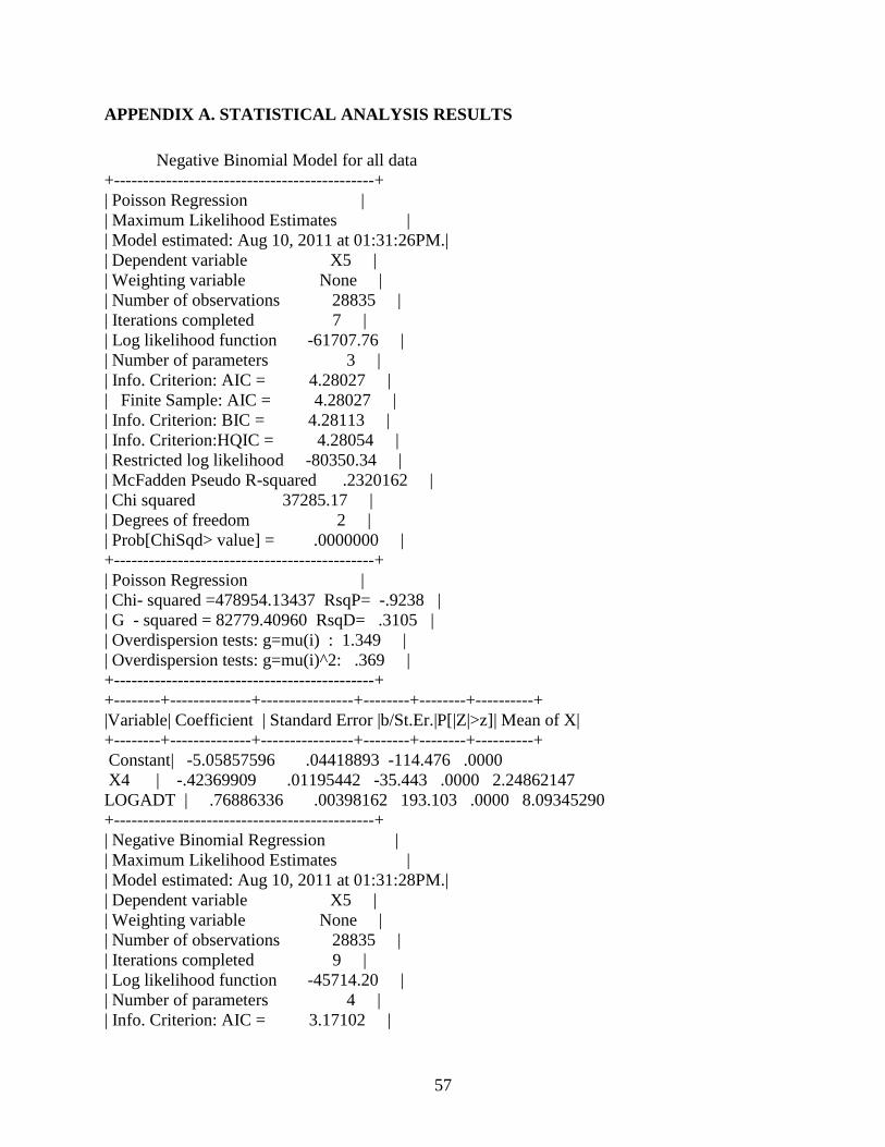
57 57
APPENDIX A. STATISTICAL ANALYSIS RESULTS
Negative Binomial Model for all data
+---------------------------------------------+
| Poisson Regression |
| Maximum Likelihood Estimates |
| Model estimated: Aug 10, 2011 at 01:31:26PM.|
| Dependent variable X5 |
| Weighting variable None |
| Number of observations 28835 |
| Iterations completed 7 |
| Log likelihood function -61707.76 |
| Number of parameters 3 |
| Info. Criterion: AIC = 4.28027 |
| Finite Sample: AIC = 4.28027 |
| Info. Criterion: BIC = 4.28113 |
| Info. Criterion:HQIC = 4.28054 |
| Restricted log likelihood -80350.34 |
| McFadden Pseudo R-squared .2320162 |
| Chi squared 37285.17 |
| Degrees of freedom 2 |
| Prob[ChiSqd> value] = .0000000 |
+---------------------------------------------+
| Poisson Regression |
| Chi- squared =478954.13437 RsqP= -.9238 |
| G - squared = 82779.40960 RsqD= .3105 |
| Overdispersion tests: g=mu(i) : 1.349 |
| Overdispersion tests: g=mu(i)^2: .369 |
+---------------------------------------------+
+--------+--------------+----------------+--------+--------+----------+
|Variable| Coefficient | Standard Error |b/St.Er.|P[|Z|>z]| Mean of X|
+--------+--------------+----------------+--------+--------+----------+
Constant| -5.05857596 .04418893 -114.476 .0000
X4 | -.42369909 .01195442 -35.443 .0000 2.24862147
LOGADT | .76886336 .00398162 193.103 .0000 8.09345290
+---------------------------------------------+
| Negative Binomial Regression |
| Maximum Likelihood Estimates |
| Model estimated: Aug 10, 2011 at 01:31:28PM.|
| Dependent variable X5 |
| Weighting variable None |
| Number of observations 28835 |
| Iterations completed 9 |
| Log likelihood function -45714.20 |
| Number of parameters 4 |
| Info. Criterion: AIC = 3.17102 |

58 58
| Finite Sample: AIC = 3.17102 |
| Info. Criterion: BIC = 3.17217 |
| Info. Criterion:HQIC = 3.17139 |
| Restricted log likelihood -61707.76 |
| McFadden Pseudo R-squared .2591822 |
| Chi squared 31987.11 |
| Degrees of freedom 1 |
| Prob[ChiSqd> value] = .0000000 |
| NegBin form 2; Psi(i) = theta |
+---------------------------------------------+
+--------+--------------+----------------+--------+--------+----------+
|Variable| Coefficient | Standard Error |b/St.Er.|P[|Z|>z]| Mean of X|
+--------+--------------+----------------+--------+--------+----------+
Constant| -5.38145833 .03959308 -135.919 .0000
X4 | -1.29146309 .01743908 -16.713 .0000 2.24862147
LOGADT | .77074842 .00340283 226.502 .0000 8.09345290
---------+Dispersion parameter for count data model
Alpha | 1.26899021 .01547431 82.006 .0000
Model for ACI≤1.5
+---------------------------------------------+
| Poisson Regression |
| Maximum Likelihood Estimates |
| Model estimated: Aug 10, 2011 at 01:43:00PM.|
| Dependent variable X5 |
| Weighting variable None |
| Number of observations 906 |
| Iterations completed 7 |
| Log likelihood function -3998.108 |
| Number of parameters 3 |
| Info. Criterion: AIC = 8.83247 |
| Finite Sample: AIC = 8.83250 |
| Info. Criterion: BIC = 8.84839 |
| Info. Criterion:HQIC = 8.83855 |
| Restricted log likelihood -5067.105 |
| McFadden Pseudo R-squared .2109680 |
| Chi squared 2137.994 |
| Degrees of freedom 2 |
| Prob[ChiSqd> value] = .0000000 |
+---------------------------------------------+
| Poisson Regression |
| Chi- squared =111502.72930 RsqP= -6.5568 |
| G - squared = 6314.96551 RsqD= .2529 |
| Overdispersion tests: g=mu(i) : 1.068 |
| Overdispersion tests: g=mu(i)^2: .086 |
+---------------------------------------------+
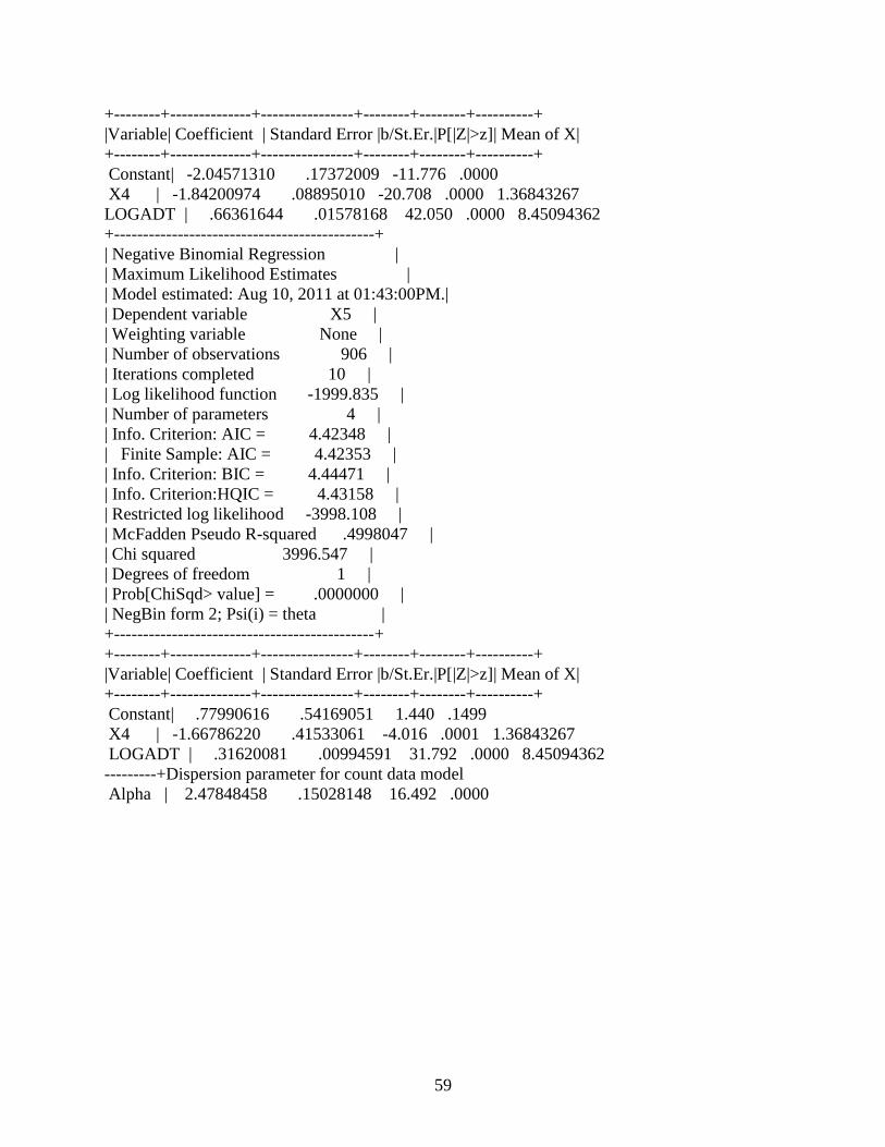
59 59
+--------+--------------+----------------+--------+--------+----------+
|Variable| Coefficient | Standard Error |b/St.Er.|P[|Z|>z]| Mean of X|
+--------+--------------+----------------+--------+--------+----------+
Constant| -2.04571310 .17372009 -11.776 .0000
X4 | -1.84200974 .08895010 -20.708 .0000 1.36843267
LOGADT | .66361644 .01578168 42.050 .0000 8.45094362
+---------------------------------------------+
| Negative Binomial Regression |
| Maximum Likelihood Estimates |
| Model estimated: Aug 10, 2011 at 01:43:00PM.|
| Dependent variable X5 |
| Weighting variable None |
| Number of observations 906 |
| Iterations completed 10 |
| Log likelihood function -1999.835 |
| Number of parameters 4 |
| Info. Criterion: AIC = 4.42348 |
| Finite Sample: AIC = 4.42353 |
| Info. Criterion: BIC = 4.44471 |
| Info. Criterion:HQIC = 4.43158 |
| Restricted log likelihood -3998.108 |
| McFadden Pseudo R-squared .4998047 |
| Chi squared 3996.547 |
| Degrees of freedom 1 |
| Prob[ChiSqd> value] = .0000000 |
| NegBin form 2; Psi(i) = theta |
+---------------------------------------------+
+--------+--------------+----------------+--------+--------+----------+
|Variable| Coefficient | Standard Error |b/St.Er.|P[|Z|>z]| Mean of X|
+--------+--------------+----------------+--------+--------+----------+
Constant| .77990616 .54169051 1.440 .1499
X4 | -1.66786220 .41533061 -4.016 .0001 1.36843267
LOGADT | .31620081 .00994591 31.792 .0000 8.45094362
---------+Dispersion parameter for count data model
Alpha | 2.47848458 .15028148 16.492 .0000
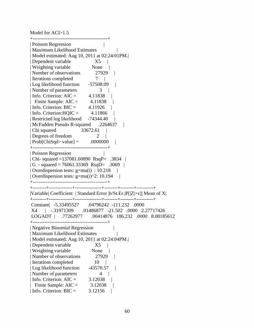
60 60
Model for ACI>1.5
+---------------------------------------------+
| Poisson Regression |
| Maximum Likelihood Estimates |
| Model estimated: Aug 10, 2011 at 02:24:01PM.|
| Dependent variable X5 |
| Weighting variable None |
| Number of observations 27929 |
| Iterations completed 7 |
| Log likelihood function -57508.09 |
| Number of parameters 3 |
| Info. Criterion: AIC = 4.11838 |
| Finite Sample: AIC = 4.11838 |
| Info. Criterion: BIC = 4.11926 |
| Info. Criterion:HQIC = 4.11866 |
| Restricted log likelihood -74344.40 |
| McFadden Pseudo R-squared .2264637 |
| Chi squared 33672.61 |
| Degrees of freedom 2 |
| Prob[ChiSqd> value] = .0000000 |
+---------------------------------------------+
| Poisson Regression |
| Chi- squared =137081.60890 RsqP= .3834 |
| G - squared = 76061.33369 RsqD= .3069 |
| Overdispersion tests: g=mu(i) : 10.218 |
| Overdispersion tests: g=mu(i)^2: 10.194 |
+---------------------------------------------+
+--------+--------------+----------------+--------+--------+----------+
|Variable| Coefficient | Standard Error |b/St.Er.|P[|Z|>z]| Mean of X|
+--------+--------------+----------------+--------+--------+----------+
Constant| -5.33495527 .04796242 -111.232 .0000
X4 | -.31971309 .01486877 -21.502 .0000 2.27717426
LOGADT | .77262977 .00414876 186.232 .0000 8.08185612
+---------------------------------------------+
| Negative Binomial Regression |
| Maximum Likelihood Estimates |
| Model estimated: Aug 10, 2011 at 02:24:04PM.|
| Dependent variable X5 |
| Weighting variable None |
| Number of observations 27929 |
| Iterations completed 10 |
| Log likelihood function -43570.57 |
| Number of parameters 4 |
| Info. Criterion: AIC = 3.12038 |
| Finite Sample: AIC = 3.12038 |
| Info. Criterion: BIC = 3.12156 |
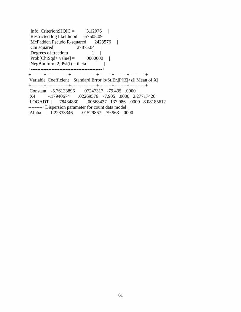
61 61
| Info. Criterion:HQIC = 3.12076 |
| Restricted log likelihood -57508.09 |
| McFadden Pseudo R-squared .2423576 |
| Chi squared 27875.04 |
| Degrees of freedom 1 |
| Prob[ChiSqd> value] = .0000000 |
| NegBin form 2; Psi(i) = theta |
+---------------------------------------------+
+--------+--------------+----------------+--------+--------+----------+
|Variable| Coefficient | Standard Error |b/St.Er.|P[|Z|>z]| Mean of X|
+--------+--------------+----------------+--------+--------+----------+
Constant| -5.76123896 .07247317 -79.495 .0000
X4 | -.17940674 .02269576 -7.905 .0000 2.27717426
LOGADT | .78434830 .00568427 137.986 .0000 8.08185612
---------+Dispersion parameter for count data model
Alpha | 1.22333346 .01529867 79.963 .0000

APPENDIX B. ECONOMIC ANALYSIS
Table B.1. Reduced number of crashes by severity
Alternatives
Crashes
Reduced
Crash Fatal (K)
Disabling
Injury (A)
Evident
Injury (B)
Possible
Injury (C) PDO (O)
Reconstruction 1.520 0.0182 0.0578 0.1474 0.3435 0.9515
Major 1.515 0.0182 0.0576 0.1470 0.3424 0.9484
Minor 1.487 0.0178 0.0565 0.1442 0.3361 0.9309
Paint 0.040 0.0005 0.0015 0.0039 0.0090 0.0250
Durable 0.151 0.0018 0.0057 0.0146 0.0341 0.0945
Tape 0.202 0.0024 0.0077 0.0196 0.0457 0.1265
Table B.2. Benefit from reduced numbers of crashes
Alternatives
Benefit
Fatal (K)
Disabling
Injury (A)
Evident
Injury (B)
Possible
Injury (C) PDO (O) Benefit (2007) Benefit (2011)
Reconstruction $63,840.00 $13,862.40 $7,077.12 $8,588.00 $2,569.10 95,936.62 $112,232.28
Major $63,630.00 $13,816.80 $7,053.84 $8,559.75 $2,560.65 $95,621.04 $111,863.10
Minor $62,454.00 $13,561.44 $6,923.47 $8,401.55 $2,513.33 $93,853.79 $109,795.66
Paint $1,680.00 $364.80 $186.24 $226.00 $67.61 $2,524.65 $2,953.48
Durable $6,342.00 $1,377.12 $703.06 $853.15 $255.22 $9,530.55 $11,149.39
Tape $8,484.00 $1,842.24 $940.51 $1,141.30 $341.42 $12,749.47 $14,915.08
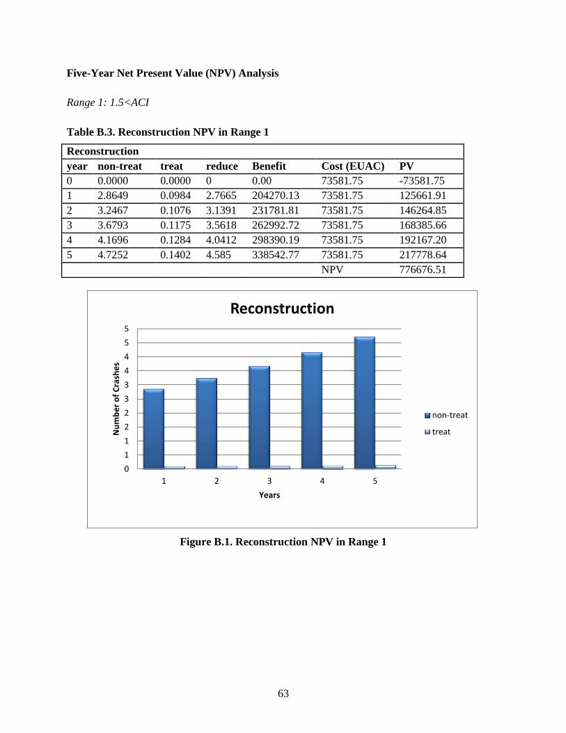
63
Five-Year Net Present Value (NPV) Analysis
Range 1: 1.5<ACI
Table B.3. Reconstruction NPV in Range 1
Reconstruction
year non-treat treat reduce Benefit Cost (EUAC) PV
0 0.0000 0.0000 0 0.00 73581.75 -73581.75
1 2.8649 0.0984 2.7665 204270.13 73581.75 125661.91
2 3.2467 0.1076 3.1391 231781.81 73581.75 146264.85
3 3.6793 0.1175 3.5618 262992.72 73581.75 168385.66
4 4.1696 0.1284 4.0412 298390.19 73581.75 192167.20
5 4.7252 0.1402 4.585 338542.77 73581.75 217778.64
NPV 776676.51
Figure B.1. Reconstruction NPV in Range 1
0
1
1
2
2
3
3
4
4
5
5
1 2 3 4 5
Nu
mb
er
of
Cra
she
s
Years
Reconstruction
non-treat
treat
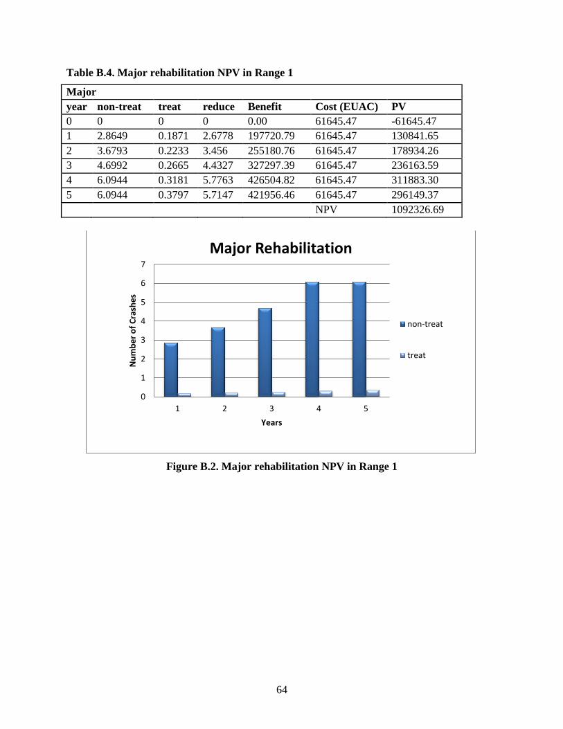
64
Table B.4. Major rehabilitation NPV in Range 1
Major
year non-treat treat reduce Benefit Cost (EUAC) PV
0 0 0 0 0.00 61645.47 -61645.47
1 2.8649 0.1871 2.6778 197720.79 61645.47 130841.65
2 3.6793 0.2233 3.456 255180.76 61645.47 178934.26
3 4.6992 0.2665 4.4327 327297.39 61645.47 236163.59
4 6.0944 0.3181 5.7763 426504.82 61645.47 311883.30
5 6.0944 0.3797 5.7147 421956.46 61645.47 296149.37
NPV 1092326.69
Figure B.2. Major rehabilitation NPV in Range 1
0
1
2
3
4
5
6
7
1 2 3 4 5
Nu
mb
er
of
Cra
she
s
Years
Major Rehabilitation
non-treat
treat
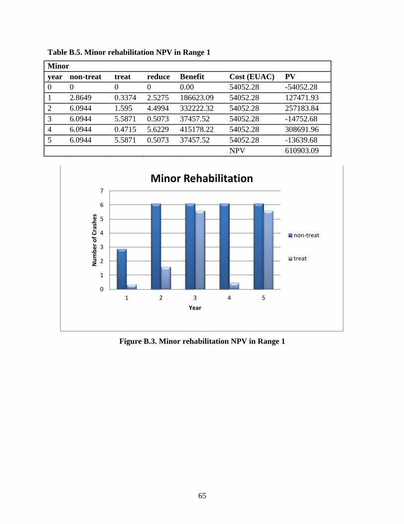
65
Table B.5. Minor rehabilitation NPV in Range 1
Minor
year non-treat treat reduce Benefit Cost (EUAC) PV
0 0 0 0 0.00 54052.28 -54052.28
1 2.8649 0.3374 2.5275 186623.09 54052.28 127471.93
2 6.0944 1.595 4.4994 332222.32 54052.28 257183.84
3 6.0944 5.5871 0.5073 37457.52 54052.28 -14752.68
4 6.0944 0.4715 5.6229 415178.22 54052.28 308691.96
5 6.0944 5.5871 0.5073 37457.52 54052.28 -13639.68
NPV 610903.09
Figure B.3. Minor rehabilitation NPV in Range 1
0
1
2
3
4
5
6
7
1 2 3 4 5
Nu
mb
er
of
Cra
she
s
Year
Minor Rehabilitation
non-treat
treat
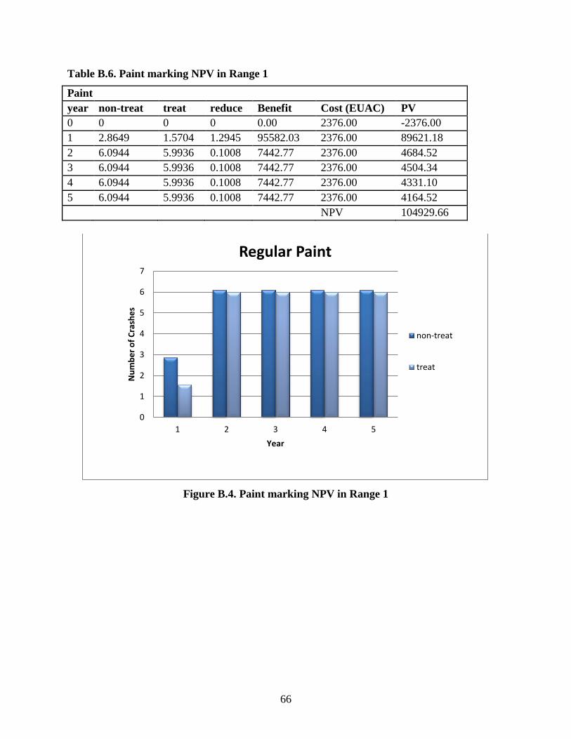
66
Table B.6. Paint marking NPV in Range 1
Paint
year non-treat treat reduce Benefit Cost (EUAC) PV
0 0 0 0 0.00 2376.00 -2376.00
1 2.8649 1.5704 1.2945 95582.03 2376.00 89621.18
2 6.0944 5.9936 0.1008 7442.77 2376.00 4684.52
3 6.0944 5.9936 0.1008 7442.77 2376.00 4504.34
4 6.0944 5.9936 0.1008 7442.77 2376.00 4331.10
5 6.0944 5.9936 0.1008 7442.77 2376.00 4164.52
NPV 104929.66
Figure B.4. Paint marking NPV in Range 1
0
1
2
3
4
5
6
7
1 2 3 4 5
Nu
mb
er
of
Cra
she
s
Year
Regular Paint
non-treat
treat
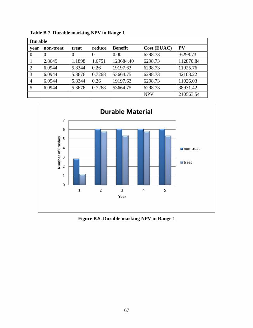
67
Table B.7. Durable marking NPV in Range 1
Durable
year non-treat treat reduce Benefit Cost (EUAC) PV
0 0 0 0 0.00 6298.73 -6298.73
1 2.8649 1.1898 1.6751 123684.40 6298.73 112870.84
2 6.0944 5.8344 0.26 19197.63 6298.73 11925.76
3 6.0944 5.3676 0.7268 53664.75 6298.73 42108.22
4 6.0944 5.8344 0.26 19197.63 6298.73 11026.03
5 6.0944 5.3676 0.7268 53664.75 6298.73 38931.42
NPV 210563.54
Figure B.5. Durable marking NPV in Range 1
0
1
2
3
4
5
6
7
1 2 3 4 5
Nu
mb
er
of
Cra
she
s
Year
Durable Material
non-treat
treat
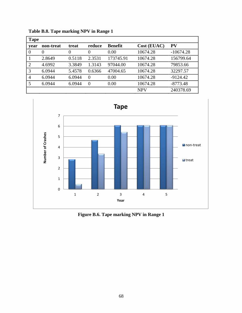
68
Table B.8. Tape marking NPV in Range 1
Tape
year non-treat treat reduce Benefit Cost (EUAC) PV
0 0 0 0 0.00 10674.28 -10674.28
1 2.8649 0.5118 2.3531 173745.91 10674.28 156799.64
2 4.6992 3.3849 1.3143 97044.00 10674.28 79853.66
3 6.0944 5.4578 0.6366 47004.65 10674.28 32297.57
4 6.0944 6.0944 0 0.00 10674.28 -9124.42
5 6.0944 6.0944 0 0.00 10674.28 -8773.48
NPV 240378.69
Figure B.6. Tape marking NPV in Range 1
0
1
2
3
4
5
6
7
1 2 3 4 5
Nu
mb
er
of
Cra
she
s
Year
Tape
non-treat
treat
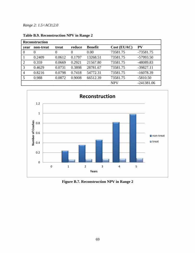
69
Range 2: 1.5<ACI≤2.0
Table B.9. Reconstruction NPV in Range 2
Reconstruction
year non-treat treat reduce Benefit Cost (EUAC) PV
0 0 0 0 0.00 73581.75 -73581.75
1 0.2409 0.0612 0.1797 13268.51 73581.75 -57993.50
2 0.359 0.0669 0.2921 21567.80 73581.75 -48089.83
3 0.4629 0.0731 0.3898 28781.67 73581.75 -39827.11
4 0.8216 0.0798 0.7418 54772.31 73581.75 -16078.39
5 0.988 0.0872 0.9008 66512.39 73581.75 -5810.50
NPV -241381.06
Figure B.7. Reconstruction NPV in Range 2
0
0.2
0.4
0.6
0.8
1
1.2
0 1 2 3 4 5
Nu
mb
er
of
Cra
she
s
Years
Reconstruction
non-treat
treat
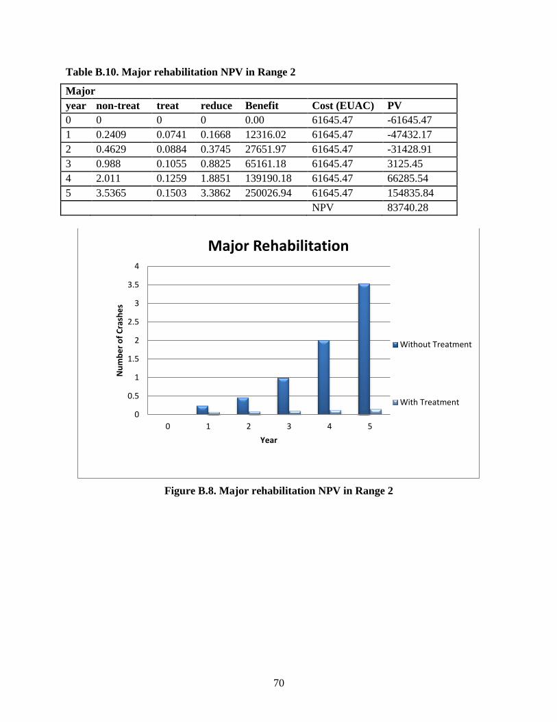
70
Table B.10. Major rehabilitation NPV in Range 2
Major
year non-treat treat reduce Benefit Cost (EUAC) PV
0 0 0 0 0.00 61645.47 -61645.47
1 0.2409 0.0741 0.1668 12316.02 61645.47 -47432.17
2 0.4629 0.0884 0.3745 27651.97 61645.47 -31428.91
3 0.988 0.1055 0.8825 65161.18 61645.47 3125.45
4 2.011 0.1259 1.8851 139190.18 61645.47 66285.54
5 3.5365 0.1503 3.3862 250026.94 61645.47 154835.84
NPV 83740.28
Figure B.8. Major rehabilitation NPV in Range 2
0
0.5
1
1.5
2
2.5
3
3.5
4
0 1 2 3 4 5
Nu
mb
er
of
Cra
she
s
Year
Major Rehabilitation
Without Treatment
With Treatment
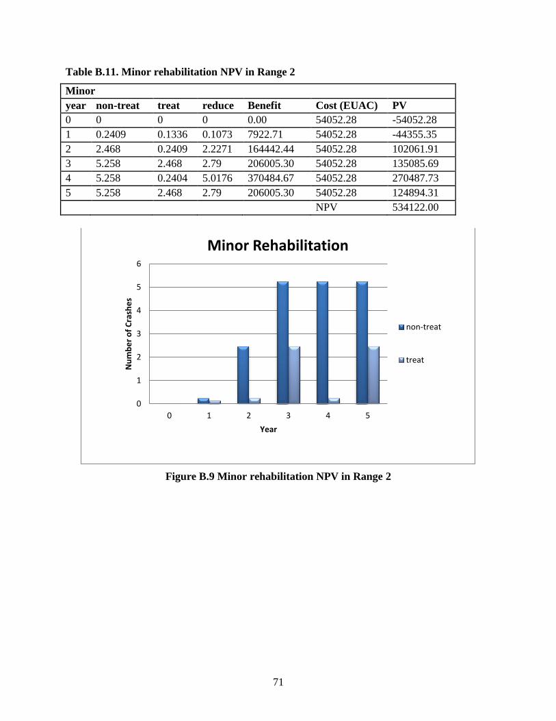
71
Table B.11. Minor rehabilitation NPV in Range 2
Minor
year non-treat treat reduce Benefit Cost (EUAC) PV
0 0 0 0 0.00 54052.28 -54052.28
1 0.2409 0.1336 0.1073 7922.71 54052.28 -44355.35
2 2.468 0.2409 2.2271 164442.44 54052.28 102061.91
3 5.258 2.468 2.79 206005.30 54052.28 135085.69
4 5.258 0.2404 5.0176 370484.67 54052.28 270487.73
5 5.258 2.468 2.79 206005.30 54052.28 124894.31
NPV 534122.00
Figure B.9 Minor rehabilitation NPV in Range 2
0
1
2
3
4
5
6
0 1 2 3 4 5
Nu
mb
er
of
Cra
she
s
Year
Minor Rehabilitation
non-treat
treat
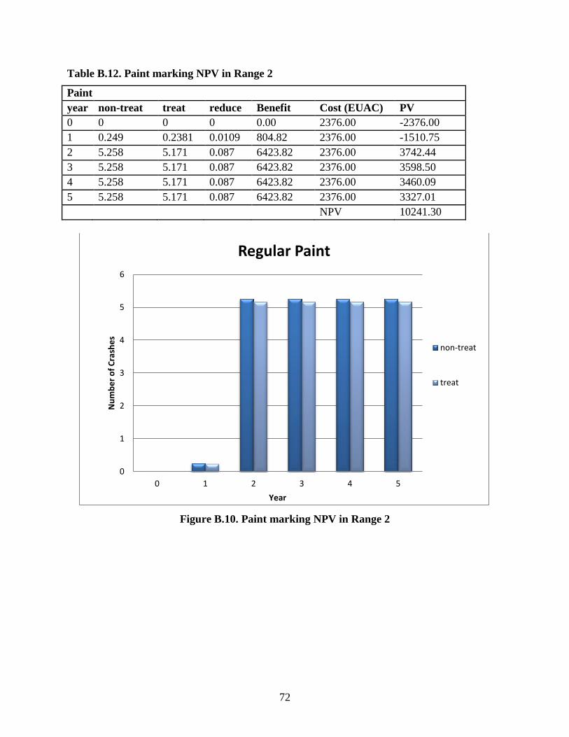
72
Table B.12. Paint marking NPV in Range 2
Paint
year non-treat treat reduce Benefit Cost (EUAC) PV
0 0 0 0 0.00 2376.00 -2376.00
1 0.249 0.2381 0.0109 804.82 2376.00 -1510.75
2 5.258 5.171 0.087 6423.82 2376.00 3742.44
3 5.258 5.171 0.087 6423.82 2376.00 3598.50
4 5.258 5.171 0.087 6423.82 2376.00 3460.09
5 5.258 5.171 0.087 6423.82 2376.00 3327.01
NPV 10241.30
Figure B.10. Paint marking NPV in Range 2
0
1
2
3
4
5
6
0 1 2 3 4 5
Nu
mb
er
of
Cra
she
s
Year
Regular Paint
non-treat
treat

73
Table B.13. Durable marking NPV in Range 2
Durable
year non-treat treat reduce Benefit Cost (EUAC) PV
0 0 0 0 0.00 6298.73 -6298.73
1 0.2409 0.2271 0.0138 1018.95 6298.73 -5076.71
2 4.2875 4.0397 0.2478 18296.82 6298.73 11092.90
3 5.258 3.7165 1.5415 113819.78 6298.73 95585.82
4 5.258 5.258 0 0.00 6298.73 -5384.18
5 5.258 4.8373 0.4207 31063.24 6298.73 20354.62
NPV 110273.72
Figure B.11. Durable marking NPV in Range 2
0
1
2
3
4
5
6
0 1 2 3 4 5
Nu
mb
er
of
Cra
she
s
Year
Durable Material
non-treat
treat
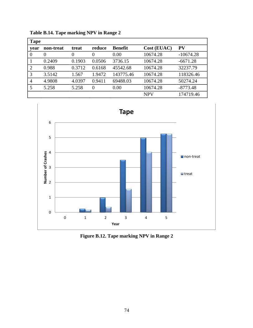
74
Table B.14. Tape marking NPV in Range 2
Tape
year non-treat treat reduce Benefit Cost (EUAC) PV
0 0 0 0 0.00 10674.28 -10674.28
1 0.2409 0.1903 0.0506 3736.15 10674.28 -6671.28
2 0.988 0.3712 0.6168 45542.68 10674.28 32237.79
3 3.5142 1.567 1.9472 143775.46 10674.28 118326.46
4 4.9808 4.0397 0.9411 69488.03 10674.28 50274.24
5 5.258 5.258 0 0.00 10674.28 -8773.48
NPV 174719.46
Figure B.12. Tape marking NPV in Range 2
0
1
2
3
4
5
6
0 1 2 3 4 5
Nu
mb
er
of
Cra
she
s
Year
Tape
non-treat
treat

75
Range 3: 2.0≤ACI<2.25
Table B.15. Reconstruction NPV in Range 3
Reconstruction
year non-treat treat reduce Benefit Cost (EUAC) PV
0 0 0 0 0.00 73581.75 -73581.75
1 0.1918 0.0708 0.121 8934.28 73581.75 -62161.03
2 0.2096 0.0773 0.1323 9768.64 73581.75 -58998.81
3 0.2289 0.0845 0.1444 10662.07 73581.75 -55935.37
4 0.2501 0.0923 0.1578 11651.48 73581.75 -52938.25
5 0.2733 0.1008 0.1725 12736.89 73581.75 -50010.04
NPV -353625.25
Figure B.13. Reconstruction NPV in Range 3
0
0.05
0.1
0.15
0.2
0.25
0.3
1 2 3 4 5
Nu
mb
er
of
Cra
she
s
Years
Reconstruction
non-treat
treat

76
Table B.16. Major rehabilitation NPV in Range 3
Major
year non-treat treat reduce Benefit Cost (EUAC) PV
0 0 0 0 0.00 61645.47 -61645.47
1 0.1918 0.0708 0.121 8934.28 61645.47 -50683.84
2 0.2289 0.0773 0.1516 11193.69 61645.47 -46645.51
3 0.2733 0.0845 0.1888 13940.43 61645.47 -42409.61
4 0.3261 0.0923 0.2338 17263.10 61645.47 -37938.24
5 0.8058 0.1008 0.705 52055.10 61645.47 -7882.58
NPV -247205.25
Figure B.14. Major rehabilitation NPV in Range 3
0
0.1
0.2
0.3
0.4
0.5
0.6
0.7
0.8
0.9
1 2 3 4 5
Nu
mb
er
of
Cra
she
s
Year
Major Rehabilitation
non-treat
treat
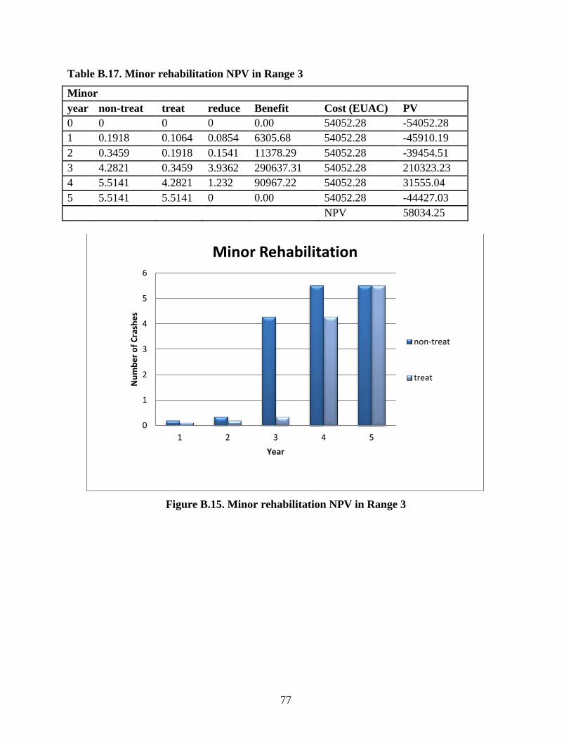
77
Table B.17. Minor rehabilitation NPV in Range 3
Minor
year non-treat treat reduce Benefit Cost (EUAC) PV
0 0 0 0 0.00 54052.28 -54052.28
1 0.1918 0.1064 0.0854 6305.68 54052.28 -45910.19
2 0.3459 0.1918 0.1541 11378.29 54052.28 -39454.51
3 4.2821 0.3459 3.9362 290637.31 54052.28 210323.23
4 5.5141 4.2821 1.232 90967.22 54052.28 31555.04
5 5.5141 5.5141 0 0.00 54052.28 -44427.03
NPV 58034.25
Figure B.15. Minor rehabilitation NPV in Range 3
0
1
2
3
4
5
6
1 2 3 4 5
Nu
mb
er
of
Cra
she
s
Year
Minor Rehabilitation
non-treat
treat
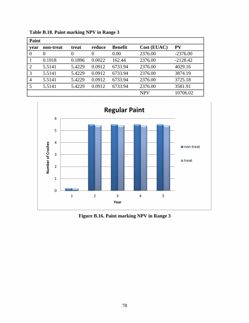
78
Table B.18. Paint marking NPV in Range 3
Paint
year non-treat treat reduce Benefit Cost (EUAC) PV
0 0 0 0 0.00 2376.00 -2376.00
1 0.1918 0.1896 0.0022 162.44 2376.00 -2128.42
2 5.5141 5.4229 0.0912 6733.94 2376.00 4029.16
3 5.5141 5.4229 0.0912 6733.94 2376.00 3874.19
4 5.5141 5.4229 0.0912 6733.94 2376.00 3725.18
5 5.5141 5.4229 0.0912 6733.94 2376.00 3581.91
NPV 10706.02
Figure B.16. Paint marking NPV in Range 3
0
1
2
3
4
5
6
1 2 3 4 5
Nu
mb
er
of
Cra
she
s
Year
Regular Paint
non-treat
treat
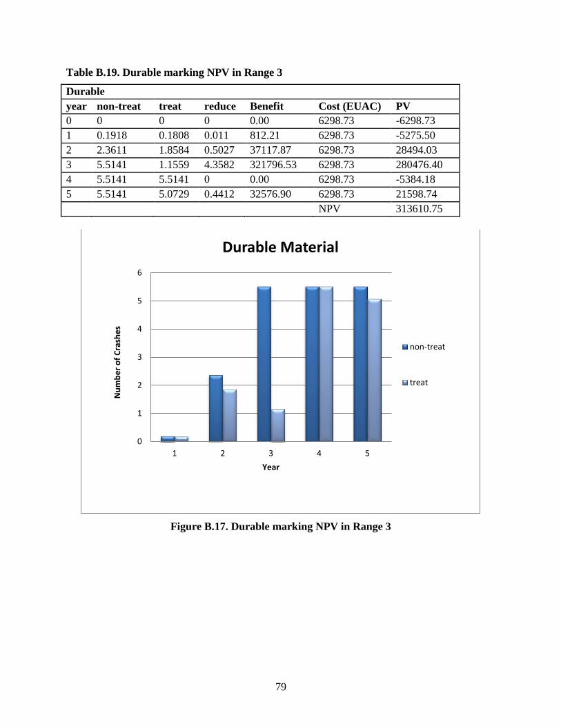
79
Table B.19. Durable marking NPV in Range 3
Durable
year non-treat treat reduce Benefit Cost (EUAC) PV
0 0 0 0 0.00 6298.73 -6298.73
1 0.1918 0.1808 0.011 812.21 6298.73 -5275.50
2 2.3611 1.8584 0.5027 37117.87 6298.73 28494.03
3 5.5141 1.1559 4.3582 321796.53 6298.73 280476.40
4 5.5141 5.5141 0 0.00 6298.73 -5384.18
5 5.5141 5.0729 0.4412 32576.90 6298.73 21598.74
NPV 313610.75
Figure B.17. Durable marking NPV in Range 3
0
1
2
3
4
5
6
1 2 3 4 5
Nu
mb
er
of
Cra
she
s
Year
Durable Material
non-treat
treat
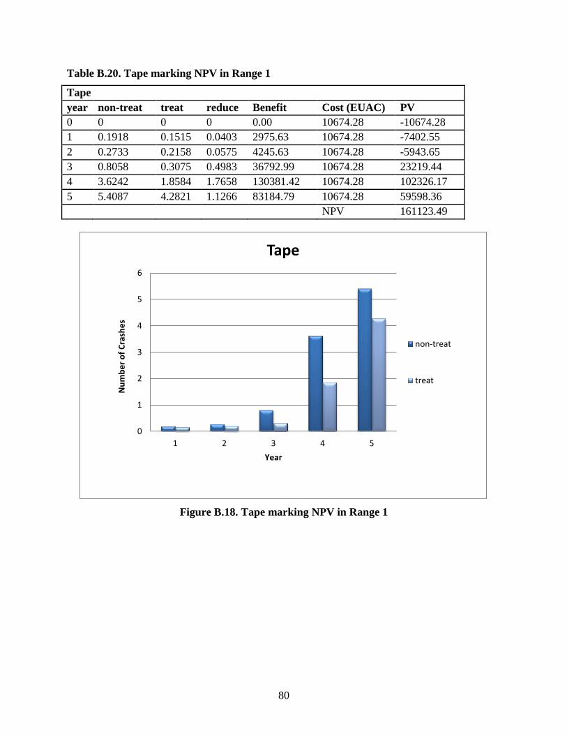
80
Table B.20. Tape marking NPV in Range 1
Tape
year non-treat treat reduce Benefit Cost (EUAC) PV
0 0 0 0 0.00 10674.28 -10674.28
1 0.1918 0.1515 0.0403 2975.63 10674.28 -7402.55
2 0.2733 0.2158 0.0575 4245.63 10674.28 -5943.65
3 0.8058 0.3075 0.4983 36792.99 10674.28 23219.44
4 3.6242 1.8584 1.7658 130381.42 10674.28 102326.17
5 5.4087 4.2821 1.1266 83184.79 10674.28 59598.36
NPV 161123.49
Figure B.18. Tape marking NPV in Range 1
0
1
2
3
4
5
6
1 2 3 4 5
Nu
mb
er
of
Cra
she
s
Year
Tape
non-treat
treat
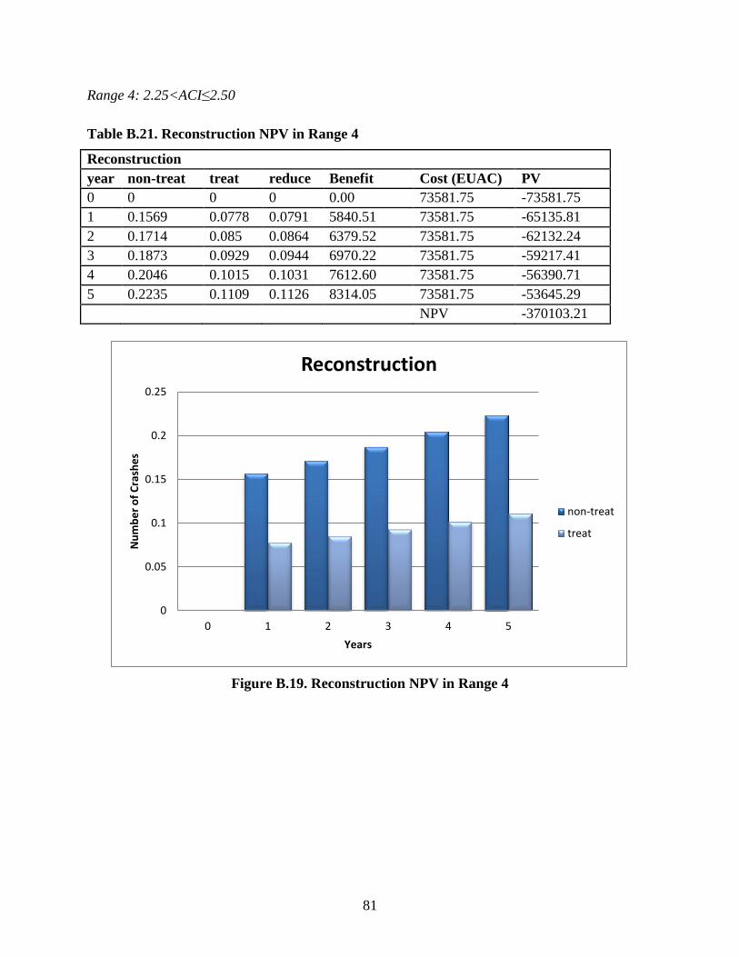
81
Range 4: 2.25<ACI≤2.50
Table B.21. Reconstruction NPV in Range 4
Reconstruction
year non-treat treat reduce Benefit Cost (EUAC) PV
0 0 0 0 0.00 73581.75 -73581.75
1 0.1569 0.0778 0.0791 5840.51 73581.75 -65135.81
2 0.1714 0.085 0.0864 6379.52 73581.75 -62132.24
3 0.1873 0.0929 0.0944 6970.22 73581.75 -59217.41
4 0.2046 0.1015 0.1031 7612.60 73581.75 -56390.71
5 0.2235 0.1109 0.1126 8314.05 73581.75 -53645.29
NPV -370103.21
Figure B.19. Reconstruction NPV in Range 4
0
0.05
0.1
0.15
0.2
0.25
0 1 2 3 4 5
Nu
mb
er
of
Cra
she
s
Years
Reconstruction
non-treat
treat
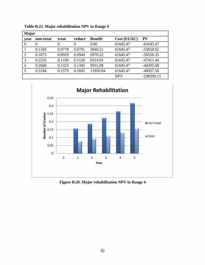
82
Table B.22. Major rehabilitation NPV in Range 4
Major
year non-treat treat reduce Benefit Cost (EUAC) PV
0 0 0 0 0.00 61645.47 -61645.47
1 0.1569 0.0778 0.0791 5840.51 61645.47 -53658.62
2 0.1873 0.0929 0.0944 6970.22 61645.47 -50550.35
3 0.2235 0.1109 0.1126 8314.05 61645.47 -47411.44
4 0.2668 0.1323 0.1345 9931.08 61645.47 -44205.68
5 0.3184 0.1579 0.1605 11850.84 61645.47 -40927.56
NPV -298399.11
Figure B.20. Major rehabilitation NPV in Range 4
0
0.05
0.1
0.15
0.2
0.25
0.3
0.35
0 1 2 3 4 5
Nu
mb
er
of
Cra
she
s
Year
Major Rehabilitation
non-treat
treat
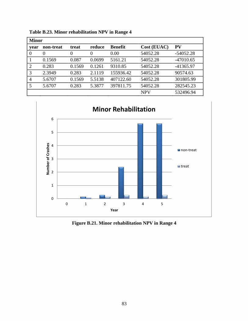
83
Table B.23. Minor rehabilitation NPV in Range 4
Minor
year non-treat treat reduce Benefit Cost (EUAC) PV
0 0 0 0 0.00 54052.28 -54052.28
1 0.1569 0.087 0.0699 5161.21 54052.28 -47010.65
2 0.283 0.1569 0.1261 9310.85 54052.28 -41365.97
3 2.3949 0.283 2.1119 155936.42 54052.28 90574.63
4 5.6707 0.1569 5.5138 407122.60 54052.28 301805.99
5 5.6707 0.283 5.3877 397811.75 54052.28 282545.23
NPV 532496.94
Figure B.21. Minor rehabilitation NPV in Range 4
0
1
2
3
4
5
6
0 1 2 3 4 5
Nu
mb
er
of
Cra
she
s
Year
Minor Rehabilitation
non-treat
treat
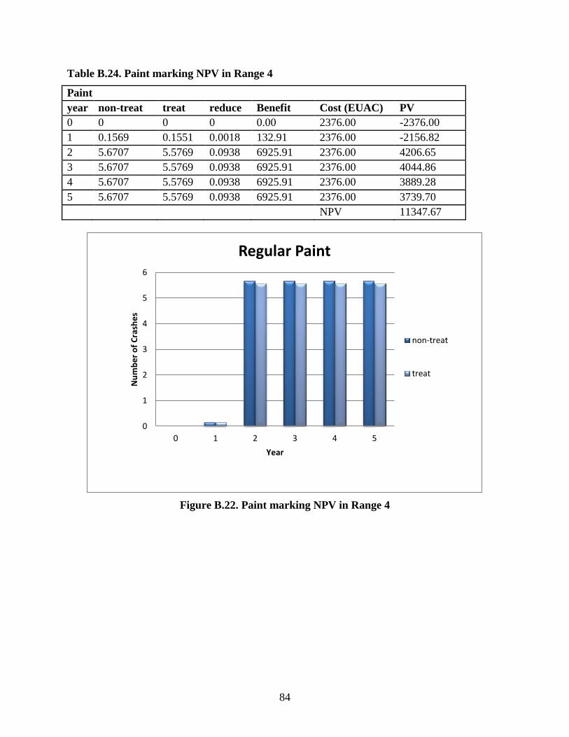
84
Table B.24. Paint marking NPV in Range 4
Paint
year non-treat treat reduce Benefit Cost (EUAC) PV
0 0 0 0 0.00 2376.00 -2376.00
1 0.1569 0.1551 0.0018 132.91 2376.00 -2156.82
2 5.6707 5.5769 0.0938 6925.91 2376.00 4206.65
3 5.6707 5.5769 0.0938 6925.91 2376.00 4044.86
4 5.6707 5.5769 0.0938 6925.91 2376.00 3889.28
5 5.6707 5.5769 0.0938 6925.91 2376.00 3739.70
NPV 11347.67
Figure B.22. Paint marking NPV in Range 4
0
1
2
3
4
5
6
0 1 2 3 4 5
Nu
mb
er
of
Cra
she
s
Year
Regular Paint
non-treat
treat
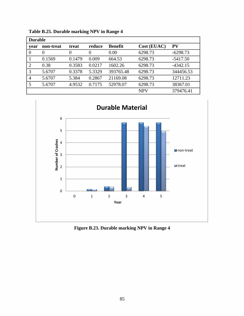
85
Table B.25. Durable marking NPV in Range 4
Durable
year non-treat treat reduce Benefit Cost (EUAC) PV
0 0 0 0 0.00 6298.73 -6298.73
1 0.1569 0.1479 0.009 664.53 6298.73 -5417.50
2 0.38 0.3583 0.0217 1602.26 6298.73 -4342.15
3 5.6707 0.3378 5.3329 393765.48 6298.73 344456.53
4 5.6707 5.384 0.2867 21169.08 6298.73 12711.23
5 5.6707 4.9532 0.7175 52978.07 6298.73 38367.01
NPV 379476.41
Figure B.23. Durable marking NPV in Range 4
0
1
2
3
4
5
6
0 1 2 3 4 5
Nu
mb
er
of
Cra
she
s
Year
Durable Material
non-treat
treat
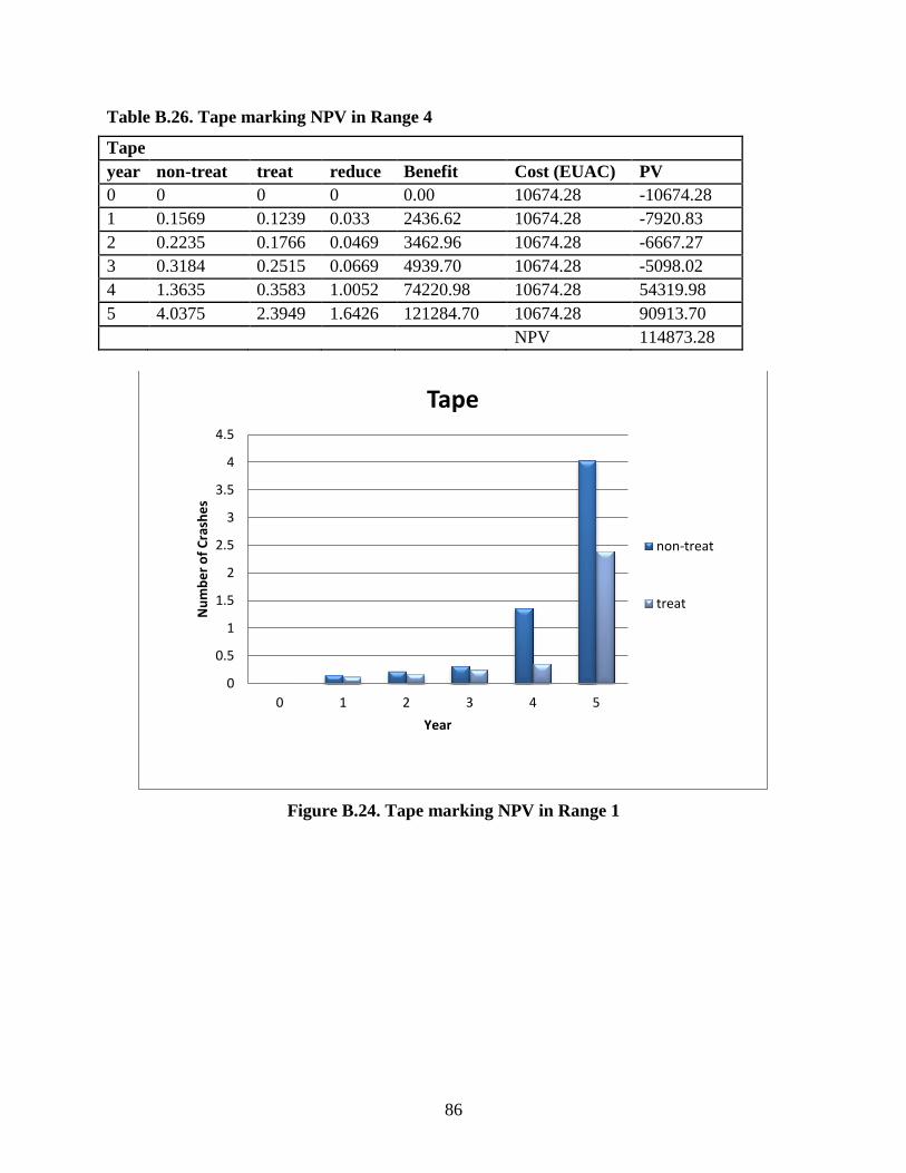
86
Table B.26. Tape marking NPV in Range 4
Tape
year non-treat treat reduce Benefit Cost (EUAC) PV
0 0 0 0 0.00 10674.28 -10674.28
1 0.1569 0.1239 0.033 2436.62 10674.28 -7920.83
2 0.2235 0.1766 0.0469 3462.96 10674.28 -6667.27
3 0.3184 0.2515 0.0669 4939.70 10674.28 -5098.02
4 1.3635 0.3583 1.0052 74220.98 10674.28 54319.98
5 4.0375 2.3949 1.6426 121284.70 10674.28 90913.70
NPV 114873.28
Figure B.24. Tape marking NPV in Range 1
0
0.5
1
1.5
2
2.5
3
3.5
4
4.5
0 1 2 3 4 5
Nu
mb
er
of
Cra
she
s
Year
Tape
non-treat
treat
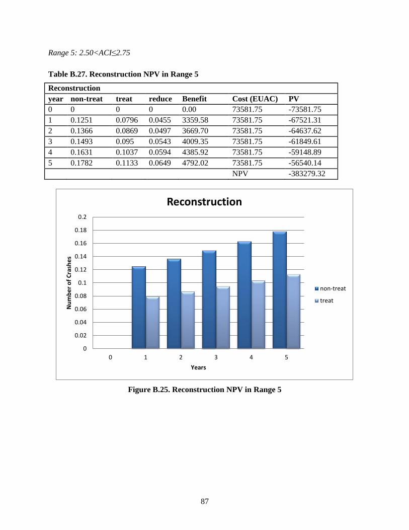
87
Range 5: 2.50<ACI≤2.75
Table B.27. Reconstruction NPV in Range 5
Reconstruction
year non-treat treat reduce Benefit Cost (EUAC) PV
0 0 0 0 0.00 73581.75 -73581.75
1 0.1251 0.0796 0.0455 3359.58 73581.75 -67521.31
2 0.1366 0.0869 0.0497 3669.70 73581.75 -64637.62
3 0.1493 0.095 0.0543 4009.35 73581.75 -61849.61
4 0.1631 0.1037 0.0594 4385.92 73581.75 -59148.89
5 0.1782 0.1133 0.0649 4792.02 73581.75 -56540.14
NPV -383279.32
Figure B.25. Reconstruction NPV in Range 5
0
0.02
0.04
0.06
0.08
0.1
0.12
0.14
0.16
0.18
0.2
0 1 2 3 4 5
Nu
mb
er
of
Cra
she
s
Years
Reconstruction
non-treat
treat
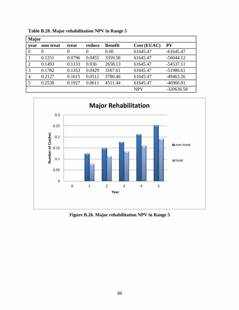
88
Table B.28. Major rehabilitation NPV in Range 5
Major
year non-treat treat reduce Benefit Cost (EUAC) PV
0 0 0 0 0.00 61645.47 -61645.47
1 0.1251 0.0796 0.0455 3359.58 61645.47 -56044.12
2 0.1493 0.1133 0.036 2658.13 61645.47 -54537.11
3 0.1782 0.1353 0.0429 3167.61 61645.47 -51986.61
4 0.2127 0.1615 0.0512 3780.46 61645.47 -49463.26
5 0.2538 0.1927 0.0611 4511.44 61645.47 -46960.01
NPV -320636.58
Figure B.26. Major rehabilitation NPV in Range 5
0
0.05
0.1
0.15
0.2
0.25
0.3
0 1 2 3 4 5
Nu
mb
er
of
Cra
she
s
Year
Major Rehabilitation
non-treat
treat
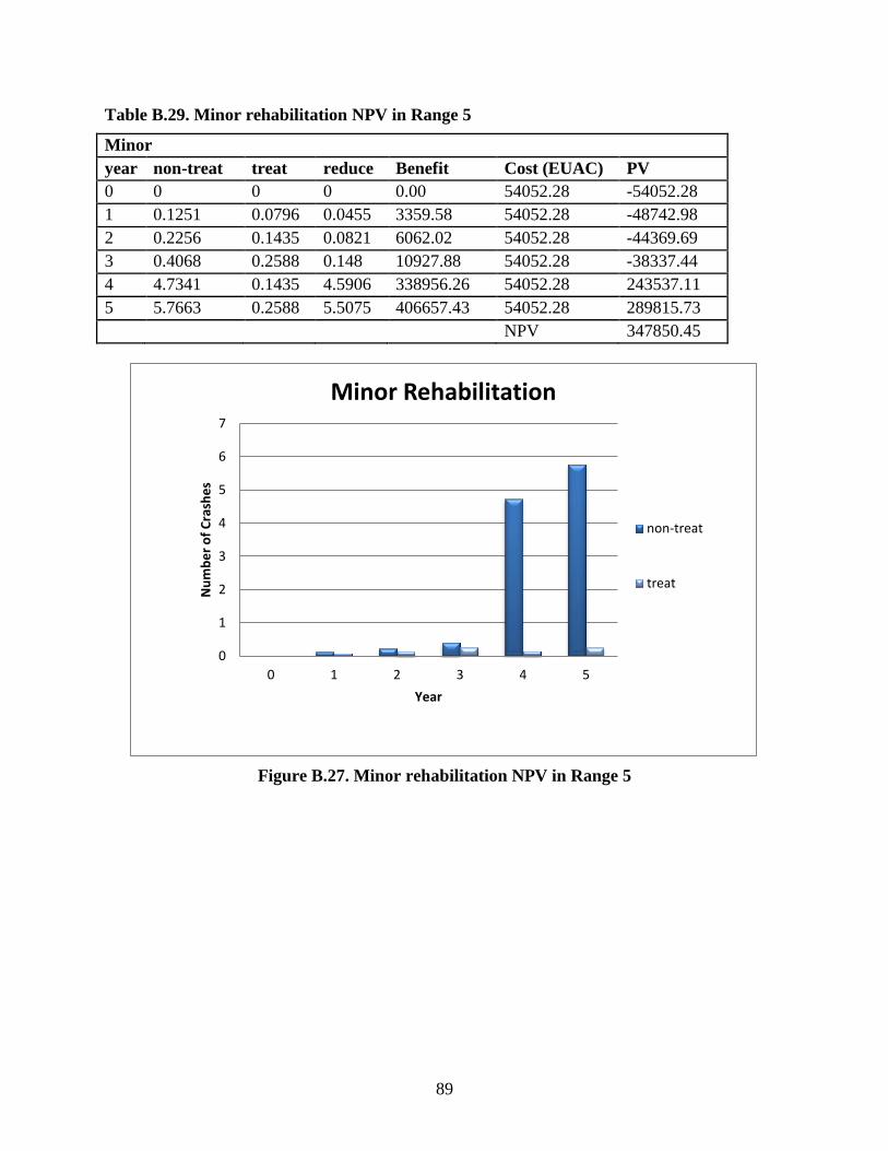
89
Table B.29. Minor rehabilitation NPV in Range 5
Minor
year non-treat treat reduce Benefit Cost (EUAC) PV
0 0 0 0 0.00 54052.28 -54052.28
1 0.1251 0.0796 0.0455 3359.58 54052.28 -48742.98
2 0.2256 0.1435 0.0821 6062.02 54052.28 -44369.69
3 0.4068 0.2588 0.148 10927.88 54052.28 -38337.44
4 4.7341 0.1435 4.5906 338956.26 54052.28 243537.11
5 5.7663 0.2588 5.5075 406657.43 54052.28 289815.73
NPV 347850.45
Figure B.27. Minor rehabilitation NPV in Range 5
0
1
2
3
4
5
6
7
0 1 2 3 4 5
Nu
mb
er
of
Cra
she
s
Year
Minor Rehabilitation
non-treat
treat
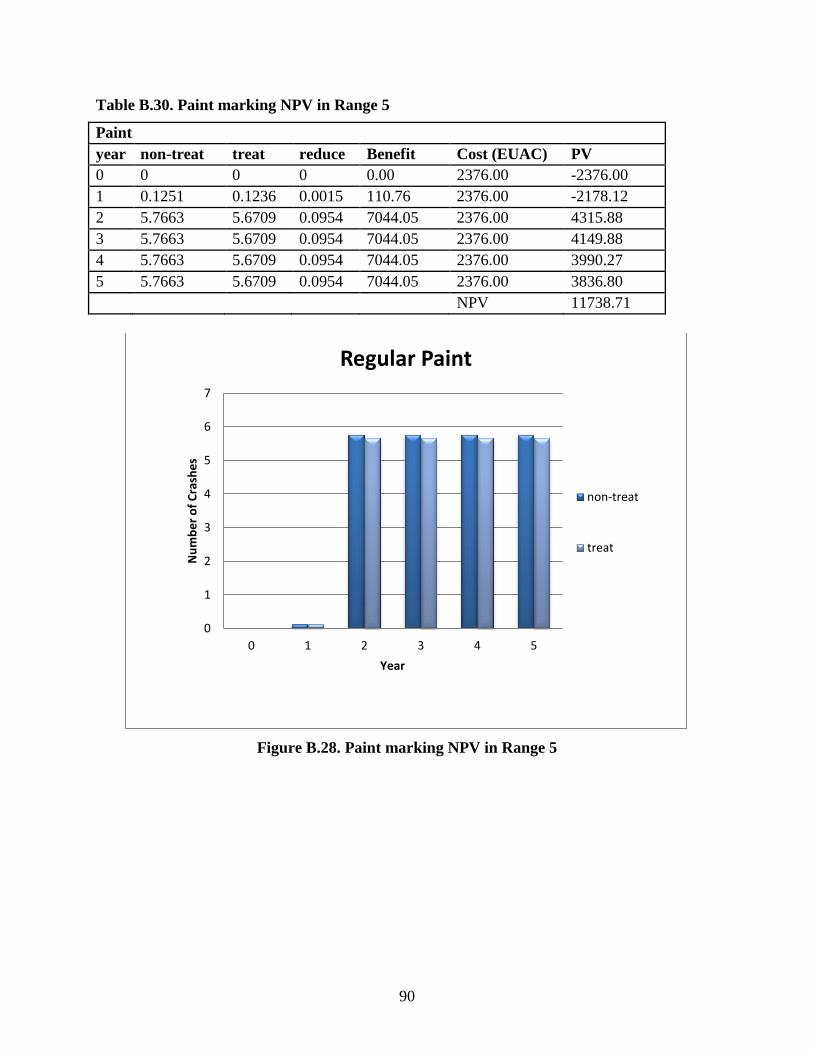
90
Table B.30. Paint marking NPV in Range 5
Paint
year non-treat treat reduce Benefit Cost (EUAC) PV
0 0 0 0 0.00 2376.00 -2376.00
1 0.1251 0.1236 0.0015 110.76 2376.00 -2178.12
2 5.7663 5.6709 0.0954 7044.05 2376.00 4315.88
3 5.7663 5.6709 0.0954 7044.05 2376.00 4149.88
4 5.7663 5.6709 0.0954 7044.05 2376.00 3990.27
5 5.7663 5.6709 0.0954 7044.05 2376.00 3836.80
NPV 11738.71
Figure B.28. Paint marking NPV in Range 5
0
1
2
3
4
5
6
7
0 1 2 3 4 5
Nu
mb
er
of
Cra
she
s
Year
Regular Paint
non-treat
treat
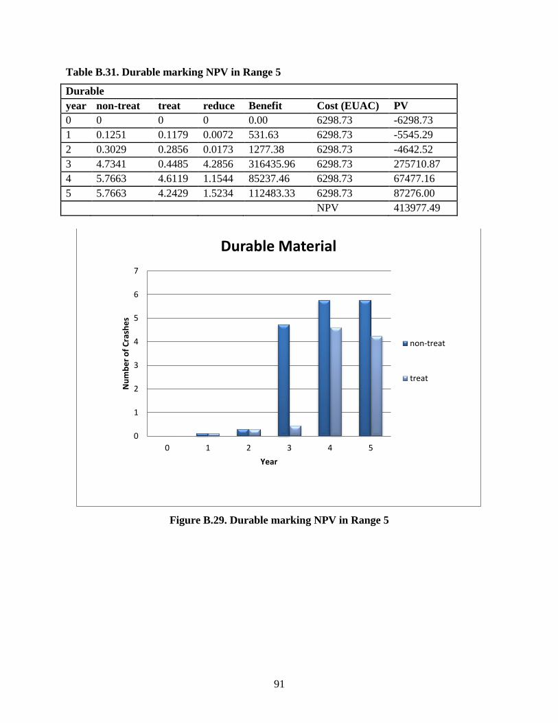
91
Table B.31. Durable marking NPV in Range 5
Durable
year non-treat treat reduce Benefit Cost (EUAC) PV
0 0 0 0 0.00 6298.73 -6298.73
1 0.1251 0.1179 0.0072 531.63 6298.73 -5545.29
2 0.3029 0.2856 0.0173 1277.38 6298.73 -4642.52
3 4.7341 0.4485 4.2856 316435.96 6298.73 275710.87
4 5.7663 4.6119 1.1544 85237.46 6298.73 67477.16
5 5.7663 4.2429 1.5234 112483.33 6298.73 87276.00
NPV 413977.49
Figure B.29. Durable marking NPV in Range 5
0
1
2
3
4
5
6
7
0 1 2 3 4 5
Nu
mb
er
of
Cra
she
s
Year
Durable Material
non-treat
treat
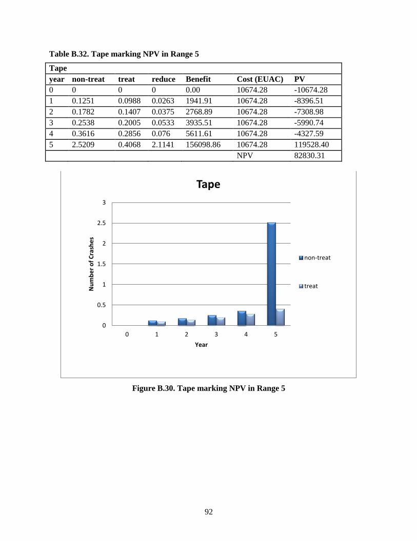
92
Table B.32. Tape marking NPV in Range 5
Tape
year non-treat treat reduce Benefit Cost (EUAC) PV
0 0 0 0 0.00 10674.28 -10674.28
1 0.1251 0.0988 0.0263 1941.91 10674.28 -8396.51
2 0.1782 0.1407 0.0375 2768.89 10674.28 -7308.98
3 0.2538 0.2005 0.0533 3935.51 10674.28 -5990.74
4 0.3616 0.2856 0.076 5611.61 10674.28 -4327.59
5 2.5209 0.4068 2.1141 156098.86 10674.28 119528.40
NPV 82830.31
Figure B.30. Tape marking NPV in Range 5
0
0.5
1
1.5
2
2.5
3
0 1 2 3 4 5
Nu
mb
er
of
Cra
she
s
Year
Tape
non-treat
treat
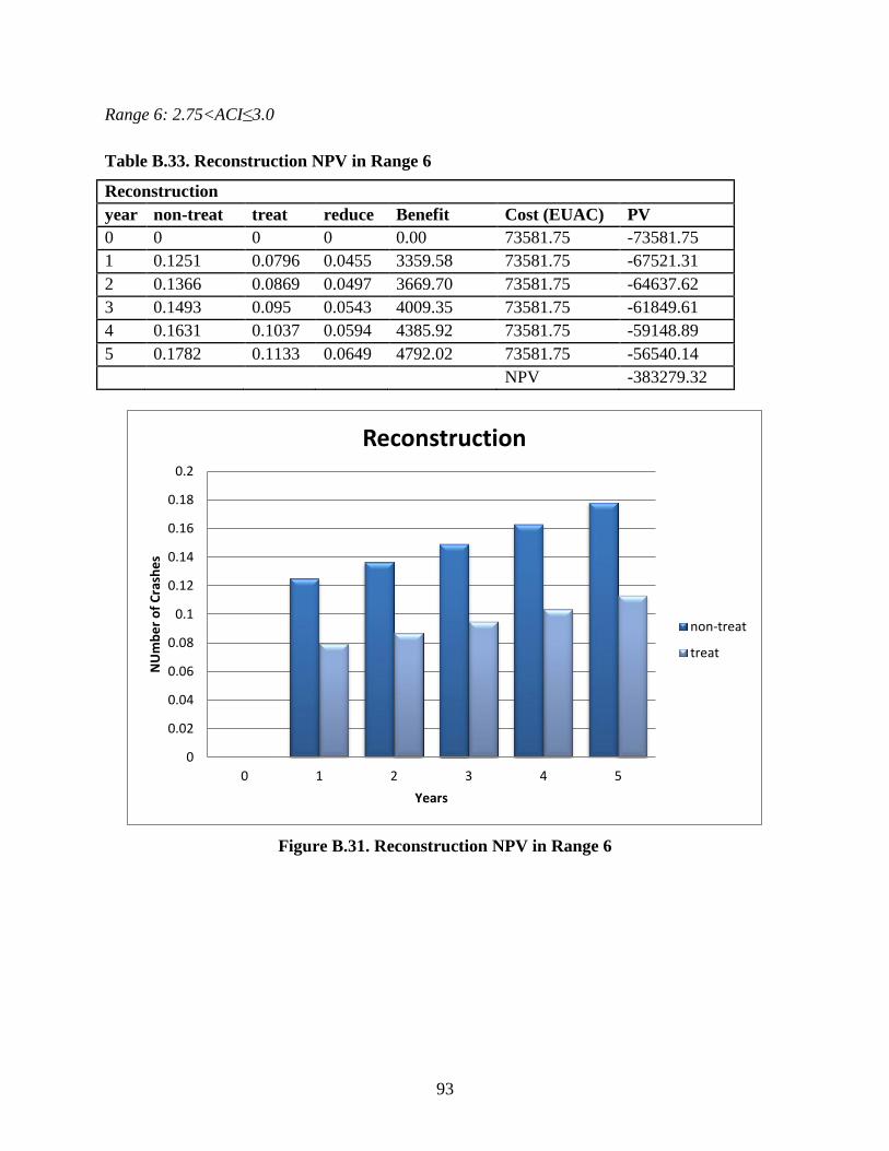
93
Range 6: 2.75<ACI≤3.0
Table B.33. Reconstruction NPV in Range 6
Reconstruction
year non-treat treat reduce Benefit Cost (EUAC) PV
0 0 0 0 0.00 73581.75 -73581.75
1 0.1251 0.0796 0.0455 3359.58 73581.75 -67521.31
2 0.1366 0.0869 0.0497 3669.70 73581.75 -64637.62
3 0.1493 0.095 0.0543 4009.35 73581.75 -61849.61
4 0.1631 0.1037 0.0594 4385.92 73581.75 -59148.89
5 0.1782 0.1133 0.0649 4792.02 73581.75 -56540.14
NPV -383279.32
Figure B.31. Reconstruction NPV in Range 6
0
0.02
0.04
0.06
0.08
0.1
0.12
0.14
0.16
0.18
0.2
0 1 2 3 4 5
NU
mb
er
of
Cra
she
s
Years
Reconstruction
non-treat
treat
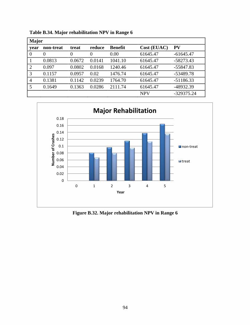
94
Table B.34. Major rehabilitation NPV in Range 6
Major
year non-treat treat reduce Benefit Cost (EUAC) PV
0 0 0 0 0.00 61645.47 -61645.47
1 0.0813 0.0672 0.0141 1041.10 61645.47 -58273.43
2 0.097 0.0802 0.0168 1240.46 61645.47 -55847.83
3 0.1157 0.0957 0.02 1476.74 61645.47 -53489.78
4 0.1381 0.1142 0.0239 1764.70 61645.47 -51186.33
5 0.1649 0.1363 0.0286 2111.74 61645.47 -48932.39
NPV -329375.24
Figure B.32. Major rehabilitation NPV in Range 6
0
0.02
0.04
0.06
0.08
0.1
0.12
0.14
0.16
0.18
0 1 2 3 4 5
Nu
mb
er
of
Cra
she
s
Year
Major Rehabilitation
non-treat
treat
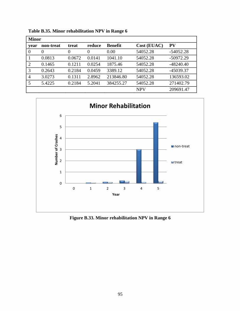
95
Table B.35. Minor rehabilitation NPV in Range 6
Minor
year non-treat treat reduce Benefit Cost (EUAC) PV
0 0 0 0 0.00 54052.28 -54052.28
1 0.0813 0.0672 0.0141 1041.10 54052.28 -50972.29
2 0.1465 0.1211 0.0254 1875.46 54052.28 -48240.40
3 0.2643 0.2184 0.0459 3389.12 54052.28 -45039.37
4 3.0273 0.1311 2.8962 213846.80 54052.28 136593.02
5 5.4225 0.2184 5.2041 384255.27 54052.28 271402.79
NPV 209691.47
Figure B.33. Minor rehabilitation NPV in Range 6
0
1
2
3
4
5
6
0 1 2 3 4 5
Nu
mb
er
of
Cra
she
s
Year
Minor Rehabilitation
non-treat
treat
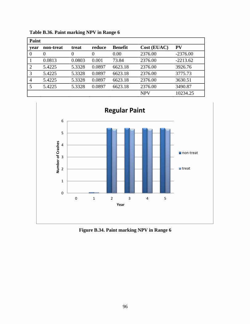
96
Table B.36. Paint marking NPV in Range 6
Paint
year non-treat treat reduce Benefit Cost (EUAC) PV
0 0 0 0 0.00 2376.00 -2376.00
1 0.0813 0.0803 0.001 73.84 2376.00 -2213.62
2 5.4225 5.3328 0.0897 6623.18 2376.00 3926.76
3 5.4225 5.3328 0.0897 6623.18 2376.00 3775.73
4 5.4225 5.3328 0.0897 6623.18 2376.00 3630.51
5 5.4225 5.3328 0.0897 6623.18 2376.00 3490.87
NPV 10234.25
Figure B.34. Paint marking NPV in Range 6
0
1
2
3
4
5
6
0 1 2 3 4 5
Nu
mb
er
of
Cra
she
s
Year
Regular Paint
non-treat
treat
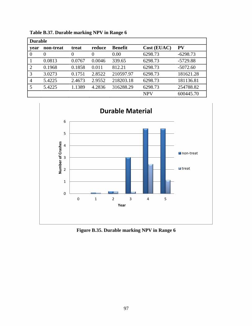
97
Table B.37. Durable marking NPV in Range 6
Durable
year non-treat treat reduce Benefit Cost (EUAC) PV
0 0 0 0 0.00 6298.73 -6298.73
1 0.0813 0.0767 0.0046 339.65 6298.73 -5729.88
2 0.1968 0.1858 0.011 812.21 6298.73 -5072.60
3 3.0273 0.1751 2.8522 210597.97 6298.73 181621.28
4 5.4225 2.4673 2.9552 218203.18 6298.73 181136.81
5 5.4225 1.1389 4.2836 316288.29 6298.73 254788.82
NPV 600445.70
Figure B.35. Durable marking NPV in Range 6
0
1
2
3
4
5
6
0 1 2 3 4 5
Nu
mb
er
of
Cra
she
s
Year
Durable Material
non-treat
treat

98
Table B.38. Tape marking NPV in Range 6
Tape
year non-treat treat reduce Benefit Cost (EUAC) PV
0 0 0 0 0.00 10674.28 -10674.28
1 0.0813 0.0672 0.0141 1041.10 10674.28 -9262.67
2 0.1157 0.0957 0.02 1476.74 10674.28 -8503.64
3 0.1649 0.1363 0.0286 2111.74 10674.28 -7612.07
4 0.2349 0.1941 0.0408 3012.55 10674.28 -6549.28
5 0.3346 0.2766 0.058 4282.55 10674.28 -5253.54
NPV -47855.48
Figure B.36. Tape marking NPV in Range 6
0
0.05
0.1
0.15
0.2
0.25
0.3
0.35
0.4
0 1 2 3 4 5
Nu
mb
er
of
Cra
she
s
Year
Tape
non-treat
treat