Embed Size (px)
Citation preview

Asset managers: Institutional performance and factor
exposures∗
Joseph Gerakos Juhani T. Linnainmaa Adair Morse
October 16, 2017
Abstract
Using a dataset of $17 trillion of assets under management, we document that actively-managed institutional accounts outperformed strategy benchmarks by 86 (42) basispoints gross (net) during 2000–2012. In return, asset managers collected $162 billionin fees per year for managing 29% of worldwide capital. Estimates from a Sharpe(1992) model imply that their outperformance comes from factor exposures (“smartbeta”). If institutions had instead implemented mean-variance portfolios of institu-tional mutual funds, they would not have earned higher Sharpe ratios. Recent growthof the ETF market implies that asset managers are losing advantages held during oursample period.
∗Gerakos is with Dartmouth College, Linnainmaa is with the University of Southern California andNBER, and Morse is with the University of California Berkeley and NBER. We thank Jules van Binsbergen(discussant), Jeff Coles (discussant), Richard Evans (discussant), Ken French (discussant), Aneel Keswani(discussant), Jonathan Lewellen, Jesper Rangvid (discussant), Scott Richardson, Julio Riutort (discussant),Clemens Sialm (discussant), Annette Vissing-Jorgensen, workshop participants at Arizona State Univer-sity, University of California at Berkeley, Emory University, University of Oregon, University of Colorado,University of Chicago, Temple University, Dartmouth College, University of Washington, Rice University,London Business School, London School of Economics, Notre Dame, University of California San Diego,the Wharton School, and conference participants at the FRIC’14: Conference on Financial Frictions, the2014 Western Finance Association Conference, the 7th International Finance Conference at the PontificiaUniversidad Catolica de Chile, the 2014 MSUFCU Conference on Financial Institutions and Investments, the2015 UBC Winter Finance Conference, the 2015 FRBNY/NYU Financial Intermediation Conference, theNBER Conference on New Developments in Long-Term Asset Management, and the 5th Luxembourg AssetManagement Summit for their comments. We thank the Fama-Miller Center at the University of ChicagoBooth School of Business for financial support.

1 Introduction
Institutions on average delegated $36 trillion in assets to asset managers between 2000 and
2012, which represents 29% worldwide investable capital. We show that asset managers
typically allocate these assets into active strategies. Institutional delegated capital therefore
represents the majority of actively managed assets. We estimate that institutions pay an
average fee of 44 basis points, or, in aggregate, $162 billion per year during our sample
period. These fees are well above the passive cost of managing and trading large portfolios
(Petajisto, 2011). In this paper, we test theories of asset management to understand why
institutions allocate their assets into active strategies. Institutions are sophisticated investors
with deliberate decision processes about delegation; if active investing is, indeed, a negative
sum game (Sharpe 1991), why do not these institutions invest all their assets passively?
We use new data on institutional assets delegated to asset managers to accomplish two
goals. We set the stage for our tests of delegation theories (our second goal) by providing
new facts about the performance of delegated institutional capital and what asset managers
do to achieve performance. We show that institutions earn positive alphas on their delegated
assets, a finding that stands in sharp contrast to estimates for retail mutual funds. Using
the (Sharpe 1992) model, we show that positive alpha emerges from managers having skill in
constructing factor portfolios. The usefulness of these skills vary by asset class and strategy,
setting up our tests of the active management theories.
Our tests of delegation to active management focus on four sets of theories. Table 1
combines these theories to convey how, in each theory, gross and net alphas and fees vary with
market inefficiency, client (investor) size or sophistication, manager size, and manager fees.
The first set of theories builds off the work of Anat Admati and Paul Pfleiderer, especially
Admati and Pfleiderer (1990). We label these theories as Delegation under Noisy Rational
Expectations. Our empirical predictions come primarily from Ross (2005) and Garcıa and
Vanden (2009), who extend the work of Adamati and Pfleiderer. In these models, agents have
1

heterogeneous signals about the value of the risky asset. In Ross’s equilibrium, all agents
whose signal precisions are above a threshold become asset managers. A single manager
with the most precise signal cannot, however, act monopolistically because additional funds,
whose managers have less precise signals, yield clients diversification benefits and can provide
their services at lower fees. The size of active management market is proportional to the
degree of informational inefficiency, and fees and manager size are informative about the
quality of the fund managers’ signals.
Second, we obtain predictions from the Perfect Competition among Investors theory of
Berk and Green (2004). This model combines decreasing returns to scale at the manager
level with perfect competition among investors. A skilled manager can either increase fees
or the size of her fund to extract all rents arising from skill. Because the investor side of the
market is perfectly competitive, investors always earn zero net alphas in expectation. Gross
returns, however, positively correlate with manager size and fees.
Third, Pastor and Stambaugh (2012) and Pedersen (2015) develop theories, which we
label Decreasing Returns to Industry Scale. These theories are similar to Berk and Green
(2004) except for the assumption that decreasing returns to scale are at the market level
and, importantly, investors can have market power. Pastor and Stambaugh (2012) focus
on the size and performance of the entire asset management industry. However, we follow
Pedersen (2015, 2017) and consider individual sectors as “markets.” That is, we consider
the possibility that the asset management market consists of different strategies, and that
the decreasing returns to scale operate at this level. The central idea in these papers is
that active management exists up to the point at which the expected skill-based alpha of an
additional dollar goes to zero.
Pastor and Stambaugh (2012) provide separate predictions depending on whether in-
vestors or managers have market power. If managers have all the power, as in Berk and
Green (2004), they share the profits among themselves and leave investors with zero net
alphas. If, by contrast, the manager side is perfectly competitive, but there is only a single
2

investor, this investor reaps all the surplus as a positive net alpha. As in Berk and Green
(2004), these models include a time-series predictions of how funds’ sizes and fees respond
to changes in the manager’s perceived skill. However, we base our predictions and empirical
analysis on the cross section.
The final theory is the recent work of Garleanu and Pedersen (2017). They combine the
assumption that investors face search costs to find skilled managers with the Noisy Rational
Expectations models assumption that active managers make money by exploiting informa-
tional inefficiencies. In Garleanu and Pedersen (2017), markets with higher information
collection costs (as in Verrecchia (1982)) exhibit more concentrated active management and
higher fees. Investors in this model can either invest in passive benchmarks or engage in
costly search for an informed manager. Investors who search for skilled managers earn posi-
tive net alphas to offset their search costs. Garleanu and Pedersen (2017) assume that more
sophisticated investors have lower search costs. Because informed managers outperform, so-
phisticated investors outperform as well. A manager’s size and client base is informative of
its ability because skilled managers have a disproportionate number of large, sophisticated
(searching) clients.
A global consultant provided us with data covering an annual average of $18 trillion in
AUM over 2000–2012.1 The data include quarterly assets and client counts, monthly re-
turns, and fee structures for 22,289 asset manager strategy funds marketed by 3,272 asset
manager firms. When an institution chooses an asset manager to delegate a strategy-level
allocation, the asset manager either sets up an investment vehicle as a segregated account or
mixes the account with a small number of institutional clients seeking the same strategy ex-
posure. Asset managers then combine all clients’ investments into pooled strategy holdings
for marketing and compliance reporting purposes. We refer to these pooled holdings as asset
1Most institutional investors use consultants in their delegation not only because of consultants’ expertisein portfolio choice, but also because consultants aggregate performance and holdings data to facilitate theshopping for asset managers (Goyal and Wahal 2008).
3

manager funds because the databases resemble the mutual fund databases. The median fund
pools six clients and has $285 million in capital invested in a strategy. Our analysis focuses
on four asset classes: U.S. fixed income (21% of delegated institutional assets), global fixed
income (27%), U.S. public equity (21%) and global public equities (31%). We show that the
database does not suffer from survivorship bias and is not biased toward better performing
funds. While delegated institutional holdings are exempt from mandatory disclosure (the
U.S. 1940 Investment Company Act covers retail delegated capital, not institutional delega-
tion), asset managers are subject to ‘GIPS Compliance’ assuring returns reporting is reliable
and always provided.
As discussed by Goyal and Wahal (2008) and Jenkinson, Jones, and Martinez (2016),
institutions typically construct their portfolios through a two-step process. Institutions first
determine their strategy-level policy allocations by optimizing over strategy-level risk and
return. Investment officers then fulfill the strategy policy allocations either “in house” or by
issuing an investment mandate to an external manager. Because portfolio risk is incorporated
at a higher level, institutions appraise fund performance along two dimensions—net alpha
and tracking error—both relative to the strategy benchmark in a single-factor model.
We find that the average asset manager fund earns an annual strategy-level gross (net)
alpha of 86 basis with a t of 3.35 (42 basis points with a t of 1.63).2 If we instead just subtract
asset class monthly performance from each fund’s performance, we find a annual market-
adjusted gross alpha of 131 basis points (t = 3.21). In dollar terms, 131 basis points of gross
alpha translates to $469 billion per year, with $307 billion accruing to institutions and $162
2This positive performance is consistent with institutions being sophisticated investors (Del Guercioand Tkac 2002), but contrasts with most studies that examine the performance of institutions (Lewellen2011). Because the unit of observation in institution-level studies includes both delegated and non-delegatedcapital, an implication of our results is that non-delegated institutional capital likely underperforms delegatedinstitutional capital. Furthermore, there are differences in asset classes covered. Most institution-level studiesfocus on the U.S. public equity asset class. In our results, U.S. public equities have the lowest positive alpharelative to strategy benchmarks. Thus, our results are consistent with Lewellen (2011) and Busse, Goyal,and Wahal (2010), who both find positive, but statistically insignificant gross alpha in U.S. public equityusing coarser data.
4

billion to asset managers. Because asset managers may take on more tracking error risk
than the rest of the market, these results do not necessarily imply that the delegated assets
of institutions earn positive risk-adjusted returns. However, a 131 basis point gross alpha
together with the adding-up constraint discussed by Sharpe (1991) implies a market-adjusted
gross alpha of all other investors of −53 basis points.3
Our detailed data allow us to infer, in the spirit of Barber, Huang, and Odean (2016) and
Berk and Binsbergen (2016), how asset managers achieve positive net alphas. The market-
ing language used by asset managers speaks of smart betas or tactical factors.4 We use the
Sharpe (1992) empirical model to construct portfolios out of tactical factors loadings that
best mimic each asset manager fund. We choose factors that nest the literature’s factor mod-
els across different asset classes. To reflect practice, we limit factors to be tradable indexes
and the weights to be long-only and to sum to one. When we estimate fund performance
compared against this mimicking portfolio, we find no excess return over the mimicking
portfolio. The fact that asset managers outperform strategy-level benchmarks but earn re-
turns comparable to the fund-level mimicking portfolios implies that asset managers provide
institutional clients with profitable systematic deviations from benchmarks.
Next, we turn to our second goal of testing theories of the delegation to active manage-
ment. To do so, we regress gross and net alphas and fees on (i) a variance measure of market
inefficiency, (ii) average client size in the fund, (iii) manager size, and (iv) manager fees. In
these regressions, we absorb monthly benchmark levels of performance or fees by including
fixed effects of strategy (or asset class) interacted with time. Our results relate to different
aspects of each theory; we therefore discuss our results by topic to describe what mechanisms
3Assuming retail mutual funds earn gross alphas close to zero (Jensen 1968; Fama and French 2010),this implies a negative gross alpha either for non-delegated retail capital, which would be consistent withCohen, Gompers, and Vuolteenaho (2002), or for non-delegated institutional capital, which would reconcileour work with Lewellen (2011).
4See, for example, Blitz (2013), Towers Watson (2013), and Jacobs and Levy (2014). Moreover, theemployees of asset managers often publish professional articles about smart beta. See, for example, Staal,Corsi, Shores, and Woida (2015), which is authored by employees of Blackrock.
5

in the data appear to be the drivers of delegation to active management.5
− The extent of price inefficiencies in a market positively relates the opportunity for
active management. Managers provide gross alphas that positively correlate with the
amount of price inefficiency. However, because managers charge fees that also positively
correlate with inefficiencies, we detect no correlation between net returns and price
inefficiency. These findings are consistent with all of the theories. This mechanism is
explicitly modeled in the noisy rational expectation theories of Admati and Pfleiderer
(1990), Ross (2005), Garcıa and Vanden (2009) and Garleanu and Pedersen (2017) as
well as Pedersen (2015).
− Decreasing returns to scale are important, reflecting ideas from Berk and Green (2004)
and later Pastor and Stambaugh (2012) and Pedersen (2017). (The ideas in these
papers have a time series element that is not yet part of our panel tests.) We find that
gross and net alphas negatively correlate with manager size. We interpret these findings
as being consistent with the discussion in Pastor and Stambaugh (2012) about how, at
times, the size of the active management industry may have grown “too large” because
investors can learn only slowly about the deterioration in alphas due to diseconomies
of scale.
− We find evidence supporting the Garleanu and Pedersen’s (2017) ideas of the fee mecha-
nism in an equilibrium matching of large managers with sophisticated clients. In their
model, the most informed managers attract more sophisticated investors who have
lower search costs to discern whether a manager is informed. These informed man-
agers grow large from their position as most informed, but may charge a lower fee; the
noise allocators in Garleanu and Pedersen (2017) choose managers randomly, and so
5In this draft of the paper, we include Table 14, which presents the empirical results that support thisdiscussion. However, the results section does not yet incorporate these empirical results and their relationwith the theories.
6

they are disproportionately the clients of uninformed managers who charge high fees.
We find that fees negatively correlate with both manager size and average client size.
− Our evidence on net alphas, however, offer a slightly different take on client market
power. An appealing way to think of the negative correlation between average client
size and fees is the bargaining power arguments in Pastor and Stambaugh (2012).
Both Pastor and Stambaugh (2012) and Garleanu and Pedersen (2017) would predict
that investor sophistication should positively correlate with net alphas if clients have
some market power, and, in addition, Garleanu and Pedersen (2017) would predict
that manager size should positively correlate with net alphas due to sorting. Our
interpretation is that bargaining happens in fees. This bargaining may take the form
of sophisticated clients negotiating lower fees with many managers, and not be of the
type of Garleanu-Pedersen “sorting” in which sophisticated clients match with the most
informed managers. The only statistically significant covariate of net alphas is manager
size. This finding appears to reflect the Berk and Green (2004) equilibrium, coupled
with the possibility that manager and industry sizes sometimes become “‘too large”
because investors slowly learn about the deterioration in alphas due to diseconomies
of scale (Pastor and Stambaugh 2012).
Several papers have been forerunners in studying agents in asset management delegation.
Jenkinson, Jones, and Martinez (2016) find that consultants’ investment recommendations
do not add value for institutions investing in U.S. actively managed equity funds. Similarly,
Goyal and Wahal (2008) find that, when pension fund sponsors replace asset managers, their
future returns are no different from the returns that they would have earned had they stayed
with the fired asset managers. Whereas these studies examine variation in performance
conditional on delegation, we build off their insights to examine the benefits of delegation.
Likewise, we build off an existing small but important literature on the returns to insti-
tutional delegation. Annaert, De Ceuster, and Van Hyfte (2005) and Bange, Khang, and
7
Miller (2008) examine the asset allocations made by twenty-six asset managers into asset
classes over time, finding performance close to benchmarks. Finally, in a large sample study,
Busse, Goyal, and Wahal (2010) examine the performance of asset managers investing in
U.S. public equities, and also fail to find performance over benchmarks.
Until recently, research on the institutional sector was at the level of institutions them-
selves, and not the capital that they delegate, because data about institutions are more
accessible Lakonishok, Shleifer, and Vishny (1992a). For example, Lewellen (2011) uses 13-
F filings to study the performance of total institutional holdings (i.e., delegated capital and
capital managed in-house) in U.S. equities and finds that institutions do not outperform
benchmarks. Likewise, there is a substantial literature about the holdings and performance
of specific types of institutions such as pensions and endowments. This literature finds mixed
results about performance.6 Because institutions both delegate capital and manage capital
in-house, one cannot make inferences about the performance of asset managers based on the
performance of institutions in general.
We also contribute to the literature on the costs of financial intermediation and the
incidence of these costs. If we apply the estimates of Philippon (2015) and Greenwood
and Scharfstein (2013) to total worldwide investable capital in 2012, the worldwide cost of
securities intermediation was $726 billion. We can compare this top-down estimate with
bottom-up calculations for costs incurred by different classes of investors. The U.S.-based
estimates of French (2008) and Bogle (2008), applied globally, imply that the intermediation
costs for retail delegation through mutual funds was approximately $100 billion for 2012.
Further, Barber, Lee, Liu, and Odean (2009)’s estimates of retail investor trading costs from
Taiwan can be scaled up to the global level and adjusted for differences in turnover, leading
6The large literature studying performance of pension funds includes Ippolito and Turner (1987), Lakon-ishok, Shleifer, and Vishny (1992b), Coggin, Fabozzi, and Rahman (1993), Christopherson, Ferson, andGlassman (1998), Blake, Lehmann, and Timmerman (1999), Del Guercio and Tkac (2002), Ferson andKhang (2002), and Dyck and Pomorski (2012). Another literature studies endowments including Brown,Garlappi, and Tiu (2010), Lerner, Schoar, and Wang (2008), and Barber and Wang (2013).
8

to an estimate of $313 billion in costs for non-delegated individual trading in 2012. We
find that institutions paid $210 billion in fees in 2012 for delegated intermediation. These
estimates leave another $100 billion to cover any asset classes omitted from these calculations
as well as institutional non-delegated trading fees. Our basis point fee estimate is consistent
with an important existing literature that documents delegation costs of approximately 50–
60 basis points for large institutions (Coles, Suay, and Woodbury 2000; Busse, Goyal, and
Wahal 2010; Dyck, Lins, and Pomorski 2013; Jenkinson, Jones, and Martinez 2016).
2 Data and descriptive statistics
We obtained a database from a large global consulting firm (the “Consultant”). Some
consultants build and maintain databases of asset manager funds. These databases look like
mutual fund databases, containing quarterly assets under management and number of clients,
current fee structures and strategy descriptions, and monthly performance of each asset
manager fund (i.e., at the strategy-level). These databases are essential to the consultants’
business model, enabling consultants to attract and service institutional clients who delegate
capital. Asset managers voluntarily report data to consultants because, in essence, the
consultants are the asset managers’ primary clients. The majority of institutional investors
use consultants to construct portfolios (Goyal and Wahal 2008).
We use the term “asset manager fund” to draw a parallel with mutual funds, although in
this setting, the word “fund” is somewhat of a misnomer. Asset managers hold institutional
capital in individual accounts or in accounts that pool small numbers of institutions. When
asset managers report institutional holdings and performance, they add up all the clients
with the same strategy focus into a single reporting vehicle (i.e., a “fund”). This fund is a
reporting vehicle, not a direct investment vehicle per se, but it conveys the performance and
holdings of the particular asset manager in the strategy in question just as mutual funds
would do in marketing.
9

The pooled strategy-level fund is also the unit used by asset managers to comply with
GIPS (Global Investment Performance Standard) reporting standards. What is now the
CFA Institute, initiated GIPS in 1987 to ensure minimum acceptable reporting standards
for investment managers. In 2005, it became the global standard. Compliance is voluntary,
but GIPS has been universally adopted by asset managers.
Because the Consultant’s business model depends on data reliability, it employs a staff
of over 100 researchers who perform regular audits of each asset manager and its funds. In
the course of these audits, the Consultant’s researchers consider the strategy placement of
the fund and verify the accuracy of the performance and holdings data. When clients shop
for asset manager funds, they can read these audits, compare the fund to benchmarks, and
read the credentials of the people running the fund. Non-reporting asset managers receive
less attention when the Consultant makes recommendations to its clients, and consultants
and investors infer any lack of reporting as a negative signal of fund quality.
2.1 Aggregate assets under management
The first column of Table 2 reports our estimates of aggregate institutional assets under
management for each year between 2000 and 2012. These estimates are based on the annual
Pensions & Investments surveys, which we describe in the Appendix.7 Total institutional
assets increased from $22 trillion in 2000 to $47 trillion in 2012, representing approximately
700 asset manager firms throughout the period (column 2). The third column reports our es-
timates of worldwide investable assets, which we detail in the Appendix. Over the 2000–2012
sample period, worldwide investable assets rose from $79 trillion to $173 trillion. The next
column shows that institutional assets held by asset managers remained relatively constant
over the sample period at approximately 29% of worldwide investable assets.
7Each year, Pensions & Investments conducts several surveys of asset managers about their assets undermanagement. These surveys are important to asset managers because they provide size rankings to potentialclients. According to Pensions & Investments, nearly all medium and large asset managers participate.
10

Important for our study is the comparison of the coverage of the Consultant’s database
with the Pensions & Investments data. The Consultant’s total assets cover 28% of institu-
tional assets under management in 2000, and rise to over 60% post-2006. In 2012, for ex-
ample, institutional assets under management in the Consultant’s database are $26 trillion,
which represented 56.1% of total institutional assets according to Pensions & Investments.
Although our data cover $26 trillion in assets under management, this amount is less
than 100% of worldwide delegated institutional assets. We therefore address the potential
for sample bias in our data. It could be that we are simply missing asset managers, who
choose not to report performance to this consultant. The Consultant’s database covers
3,500 to 4,200 asset manager firms per year. When we hand match the names of the asset
manager firms in the Consultant’s database to those in the Pensions & Investments, 82.6% of
the firms in Pensions & Investments are included in the Consultant’s database. We examined
the missing firms and found that nearly half of these firms are private wealth assets or the
assets of smaller insurance company (but not the large insurer-asset managers). Another
16% of the missing firms specialize in private equity, real estate, or other alternatives, which
represent asset classes that we do not consider. The remaining missing firms are retail banks
mostly from Italy and Spain, and boutique asset managers from the U.S., which presumably
cater to specific clients and thus do not advertise. We therefore feel comfortable that we have
close to the population of large asset managers worldwide that serve institutional clients,
except perhaps in southern Europe.
When we instead consider the possibility of selective reporting by the asset managers
included in the Consultant’s database, we consider three potential sources of bias. It could
be (i) that asset managers always exclude certain clients’ accounts, (ii) that asset managers
selectively report assets under management at points in time when returns are good, or
(iii) that they report assets under management but not the returns when performance is
good. Based on discussions with the Consultant, we infer that issue (i) accounts for most of
the missing fund-level data. In particular, the Consultant disclosed that missing from the
11

database are specialized proprietary accounts. When choosing asset managers, institutional
investors can only see funds that appear in the databases. Thus, although the data are
incomplete, they nonetheless represent an institutional investor’s information set for deciding
among asset manager funds that are open for investment.8
Nonetheless, we do not know how these missing accounts perform. Our main concern
is that manager choose to report based on fund performance. However, asset managers
cannot selectively report based on performance and be in compliance with GIPS reporting
procedures. This constraint especially binds starting in 2006, when GIPS was revised and
became the global reporting standard for asset managers. Thus, we will split the sample at
2006 to ensure that our inferences hold in the recent period.
We also can directly test for bias in reporting following Blake, Lehmann, and Tim-
merman (1999). They state on page 436 that if “bias infected the funds included in our
subsample, they should be more successful ex post than those in the overall universe.” To
implement their test, we create two variables to measure the extent that managers report
to the Consultant’s database. The first variable, coverage, is the percentage of total assets
under management for which the manager reports data to the Consultant on strategy-level
data to the Consultant. The second variable, internal coverage, is the percentage of total
reported strategy-level assets for which the manager reports returns to the Consultant. We
regress fund-level monthly returns on these two variables. We include interactions of strategy
and month fixed effects to absorb strategy-level performance and cluster standard errors at
the month-strategy level. If managers refrain from reporting strategies with worse perfor-
mance, we would expect coverage to be negatively related to performance. For example, if
a manager’s coverage is 100%, then this manager should have a lower overall return than a
manager who only reports better performing funds.
Table 2 presents results for these regressions with the first specification including coverage
8Ang, Ayala, and Goetzmann (2014) make a similar point with respect to endowments making allocationdecisions regarding alternative asset classes.
12

and second specification including both coverage and internal coverage. For both sets of
regressions, we find the opposite of what one would expect if managers selectively reported
to the Consultant’s database based on performance—managers who provide higher levels of
coverage have slightly higher performance. The estimates presented in Table 3 suggest that
our data do not suffer from survival or selection biases.
Two related concerns are survivorship and backfill biases. The Consultant’s record-
keeping, however, mitigates these concerns. Regarding backfill, the Consultant records a
“creation date” for each asset manager fund, reflecting the date the asset manager fund was
first entered into the system. At the initiation of coverage, the manager can provide historical
returns for the fund. Such backfilled returns would be biased upward if better performing
funds were more likely to survive and/or provide historical returns. In our analysis, we
always analyze returns generated after the creation date. In the last column of Table 2, we
show an annual average of 13% of the data are backfilled (and tossed), particularly in the
early years. Survivorship bias may also occur if funds that closed were removed from the
database. However, this is not the case—the Consultant leaves dead funds in the database.
2.2 Aggregate fees
The Consultant’s database includes the fee structure for each asset manager fund. For
example, one U.S. fixed income-long duration fund charges 40 basis points for investments
up to $10 million, 30 basis points for investments up to $25 million, 25 basis points for
investments up to $50 million, and 20 basis points for investments above $50 million. These
parameters are static in the sense that the database records only the latest fee schedule from
the asset manager. However, because these fees are in percent rather than dollars, the use
of the static structure should only be problematic if fees over the last decade materially
changed per unit of assets under management.
Figure 1 depicts three different estimates of aggregate fees. First, we calculate a schedule
13

middle point estimate that assumes that the average dollar in each fund pays the median fee
listed on the fund’s fee schedule. This fee estimate could, however, be too high. Institutional
investors could negotiate side deals that shift their placement in the fee schedule up. Thus,
we second calculate a fee schedule lower bound estimate, which uses the lowest fee in the
schedule for all capital invested in the fund. In the example above, we would apply the rate
20 basis points to all capital invested in the fund. The fee schedule lower bound estimate
does not, however, account for the possibility that large investors pay less than 20 basis
points. Such instances are likely limited to select clients. Nonetheless, we implement a more
conservative estimate that we call the implied realized fee. Some funds in the Consultant’s
database report both net and gross returns. These funds therefore provide an estimate of
effective fees. We annualize the monthly gross versus net return difference, take the value-
weighted average, and then re-weight the asset classes so that the weight of each asset class
matches that in the entire database.
Figure 1 plots annual estimates of aggregate fees received by asset managers for these
three measures, aggregated to the total worldwide investable assets. We aggregate by taking
the weighted average fees in the Consultant’s data and then multiplying by the estimates of
worldwide delegated institutional assets under management from Pensions & Investments.
Based on this aggregation, we estimate that fees received by the top global asset managers
range from $125 to $162 billion per year on average over the period.
2.3 Fund-level assets under management
The Consultant categorizes funds into eight broad asset classes: U.S. public equity, global
public equity, U.S. fixed income, global fixed income, hedge funds, asset blends, cash, and
other/alternatives. We drop other/alternatives, hedge funds, and asset blends because these
funds represent heterogeneous investment strategies that make benchmarking challenging.
We also drop the cash asset class because these short-term allocations play a different role in
14

portfolios. Our database starts with 44,643 asset manager funds over the period 2000–2012.
After removing funds with no returns, cash funds, asset blend funds, other/alternatives
funds, hedge funds, funds with backfilled returns, and funds that were inactive during the
sample period, the sample consists of 15,893 funds across 3,318 asset manager firms. This
sample encompasses 936,383 monthly return observations. Panel A of Table 4 reports de-
scriptive statistics on the sample. The average total assets under management (AUM) in the
sample is $9.1 trillion. In terms of age, the funds in the database are relatively established
with the average fund being 12 years old. The largest asset classes are global and U.S. public
equity with, on average, $2.7 trillion and $2.4 trillion in assets under management followed
by U.S. fixed income ($2.2 trillion) and global fixed income ($1.8 trillion).
Panel B reports descriptive statistics at the asset manager fund level. For each month,
we calculate the distributions and then take the average of the distributions. The average
fund has $1.8 billion in assets under management, and the median fund has $411 million.
The skew is due to large institutional mutual funds in the database. Hence, we focus on
median statistics. The median fund has 6.5 clients and $55.3 million AUM per client. Many
institutional investors have much smaller mandates. The 25th percentile mandate is just
under $13 million.
We next present fund-level descriptive statistics for the four broad asset classes. The
largest funds are U.S. and global fixed income, which have, on average, $2.6 billion and $2.2
billion in total AUM as of 2012, followed by global public equity ($1.7 billion) and U.S. public
equity ($1.4 billion). Assets under management per client are also larger for fixed income
funds than for equities. For example, the median per client investment in a U.S. fixed income
fund is $74 million, compared to $30.6 million for U.S. public equity. Thus, fixed income
investments are larger in fund size and mandates per client.
15

2.4 Fund-level fees
We next examine fee distributions by asset class and client size. Panel A of Table 4 reports
that the mean value-weighted fee is 44 basis points. This corresponds with the schedule
middle point estimate presented in Figure 1, which aggregates up to $162 billion if applied
to all delegated institutional assets. The value-weighted mean fee is lowest for U.S. fixed
income (28.7 basis points), followed by global fixed income (31.9 basis points), U.S. public
equity (49.2 basis points) and global public equity (48.2). The global asset classes have more
right-skew, accounting for the larger means.
A natural question arises of who pays these fees. The equal-weighted fee is 56 basis points.
Funds with lower assets under management are more expensive, as one might expect if larger
clients get price breaks. We do not observe individual client investments in each fund. We
can, however, examine the distribution of fees conditional on the fund’s average mandate
size. Panel B of Table 5 presents these conditional distributions. Fees trend downward in
assets per client. For example, when the assets per client are less than $10 million, the
value-weighted mean fee ranges from 60.9 to 66.8 basis points, but is 37 basis points or less
when the assets per client are greater than $1 billion.9
Our fee estimates are in line with those reported in both the press and academic research.
For example, Zweig (2015) reports that CalPERS paid an average fee of 48 basis points
in 2012. Coles, Suay, and Woodbury (2000) describe the fee price breaks for closed-end
institutional funds. They find that a typical fund charges 50 basis points for the first $150
million, 45 basis points for the next $100 million, 40 basis points for the subsequent $100
million, and 35 basis points allocations above $350 million. Examining active U.S. equity
institutional funds, Busse, Goyal, and Wahal (2010) find that fees are approximately 80 basis
points for investments of $10 million and approximately 60 basis points for investments of
$100 million.
9The very small mandates (less than $1 million) are likely to be in institutional mutual funds, which mayexplain why the average fees are slightly lower on the first row than on the second.
16

Beyond scale effects and the negotiating power held by large investors, asset managers
may take into account other factors to determine an institution’s willingness-to-pay, such
as the ability of institutions to manage capital in-house, behavioral biases, or agency issues
associated with delegation.10 We do not capture such factors in our analysis.
3 Results
3.1 Alpha relative to the market
We start by comparing the performance of asset managers to the overall market. Panel A
of Table 6 reports estimates of gross and net alphas from a market model that subtracts
the returns on the broad asset class benchmarks.11 We implement monthly value-weighted
regressions of asset manager fund returns on broad asset class benchmark returns, con-
straining the market beta to be equal to one. Alphas in this specification represent simple
value-weighted, monthly returns over the benchmark index. Tracking errors are defined as
the standard deviation of the residual in a model that allows for a non-zero alpha. For
exposition, we annualize alphas and tracking errors in all of our tables. We find that asset
manager funds exhibit a market-adjusted gross alpha of 131 basis points annually, with a t
of 3.21, and a net alpha of 88 basis points, with a t of 2.14.
Which asset classes account for the positive performance? The rows of Panel B report the
net alphas and portfolio weights by year and asset class, and the far right column reports the
time series of gross alphas. The bottom row reports how the asset classes each contribute
to add up to the 131 basis points. The alpha contribution comes from global equity (50
10See, for example, Lakonishok, Shleifer, and Vishny (1992b), Brown, Harlow, and Starks (1996), Chevalierand Ellison (1997), Gil-Bazo and Ruiz-Verdu (2009), and Gennaioli, Shleifer, and Vishny (2015).
11In our analysis, we use the following broad asset class benchmarks: Russell 3000 (U.S. public equity),MSCI World ex U.S. Index (global public equity), Barclays Capital U.S. Aggregate Index (U.S. fixed income),and Barclays Capital Multiverse ex US Index (global fixed income). Table A3 provides return statistics forthe benchmarks and the Consultant’s funds mapped to each asset class.
17

basis points), U.S. equity (40 basis points), U.S. fixed income (22 basis points), and global
fixed income (17 basis points). The decomposition also indicates that positive alpha is
partly driven by timing (i.e., having greater weights invested in asset classes that performed
well during that period). We can quantify the timing contribution. If asset manager funds
invested with the average weights across the asset classes (i.e., did not dynamically adjust
the asset class portfolio weights), gross alpha would have been 102 basis points. Hence, 29
basis points of alpha is due to timing across asset classes.
Given that asset managers funds earn positive alpha in a sample that encompasses over
13% of the total worldwide investable assets, the adding-up constraint argument of Sharpe
(1991) implies that the rest of the market earns negative gross alphas relative to the market.
If we assume that there is no selection bias in our data relative to the aggregate delegated
institutional capital in the Pensions & Investments surveys, we can extrapolate our esti-
mates to approximately 29% of worldwide investable assets. The market clearing constraint
suggests that if asset manager funds return a positive 131 basis points gross over the index,
everyone else must return a gross 53 basis points below the index.12
We can convert this gross alpha into dollars. Maintaining the assumption that the Con-
sultant’s database is representative of the Pensions & Investments sample, asset manager
funds collectively earn $469 billion per year from the rest of the market. Of this amount,
$162 billion accrues to asset managers in fees and $307 billion accrues to institutions. In
terms of the dollar value added measure of Berk and Binsbergen (2015), the average asset
manager fund generates $181,811 in value-added per month, which is similar to the estimates
of Berk and Binsbergen (2015) for retail equity mutual funds ($140,000 per month). Our
results together with the finding of Fama and French (2010) that retail mutual funds’ gross
alphas are close to zero suggest that asset managers earn positive alphas at the expense of
12The market clearing constraint is that the average investor holds the market, which implies thatwasset managersαasset managers + (1 − wasset managers)αeveryone else ≡ 0. We use this condition to obtain the esti-mate of αeveryone else = −53 basis points.
18
non-delegated institutional and individual investors.
3.2 Performance
As discussed by Goyal and Wahal (2008) and Jenkinson, Jones, and Martinez (2016), in-
stitutions typically construct their portfolios through a two-step process. Institutions first
determine their strategy-level policy allocations by optimizing over strategy-level risk and
return. Investment officers then fulfill strategy policy allocations either “in house” or by
issuing an investment mandate to an external manager. Because overall portfolio risk is typ-
ically incorporated in the first-step of determining strategy allocations, institutions generally
appraise fund performance relative to only the strategy benchmark. Fund performance is
commonly reported in two dimensions—net alpha and tracking error estimated in a strategy-
level factor model.13
3.2.1 Asset class benchmarked performance
To place out strategy-level benchmark results (in the next subsection) in context, we first
evaluate performance relative to broad asset class benchmarks. We regress monthly fund
returns in excess of the one-month Treasury bill on the excess return of each benchmark. We
estimate these regressions separately for funds’ gross and net returns. Our prior was that
institutions investing in asset manager funds likely have longer investment horizons than
retail investors and are thus willing to hold more market exposure (i.e., betas higher than
one in the traditional CAPM sense). Thus, we expected that the 131 basis points gross alpha
from above would decline in a factor model of performance. The data did not support our
prior. Table 7 reports that the overall (row 1) beta is less than one (0.93). Asset manager
funds exhibit gross and net alphas of 189 basis points and 145 basis points. These estimates
13Our focus on a single factor is consistent with the findings of Barber, Huang, and Odean (2016) andBerk and Binsbergen (2016), who find that mutual fund flows respond to a single-factor model rather than,for example, to multi-factor models.
19

do not, however, reflect performance from the viewpoint of an institutional investor because
the benchmark is not at the strategy level.
Nevertheless, we can compare these broad market results to those of Lewellen (2011)
and Busse, Goyal, and Wahal (2010). Using aggregate institutional holdings of U.S. public
equities taken from 13-F filings, Lewellen (2011) finds an insignificant gross alpha of 32 basis
points (annualized) in a market model. For U.S. equity asset manager funds, Busse, Goyal,
and Wahal (2010) estimate a gross alpha for U.S. equities of 64 basis points per year. Their
estimate is not statistically significant, which may be driven by differences in sample period
and their use of quarterly rather than monthly data. Lewellen’s lower estimate may be due
to the non-delegated holdings of institutions, that are not included in our sample or in that
of Busse, Goyal, and Wahal (2010).
3.2.2 Strategy benchmarked performance
The Consultant’s database classifies the asset manager funds into 170 granular strategy
classes (e.g., Australian equities is a strategy class under the broad asset class of global
public equity). In addition, the database includes a strategy-level benchmark for each fund.
The Consultant sets the benchmarks based on the suggestion of the asset manager, auditing
each strategy to ensure that the proposed benchmark is appropriate for the fund. We evaluate
performance using the modal benchmark in the strategy class. If the benchmark chosen has
less than 10% coverage of funds in the strategy, we instead use the benchmark covering
the most assets under management in the strategy. We list the 170 strategies and their
benchmarks in Table A5 of the Internet Appendix.
Panel A of Table 8 reports estimates of asset manager fund performance from the view-
point of an institutional investor; namely, performance in a strategy-level single factor model.
We find a gross alpha of 86 basis points (t = 3.35) and a net alpha of 42 basis points (t =
1.63). In this estimation, the precision of benchmarking improves materially, especially in
20

the global asset classes. The model’s explanatory power increases from 69.9% (Table 7) to
82.3% (Table 8) when we replace broad asset class benchmarks with strategy-level bench-
marks. Tracking error falls to 5.6%, which is almost identical to the Del Guercio and Tkac
(2002) estimate for pension funds and in line with Petajisto’s (2013) estimate for moderately
active retail mutual funds.14 Our beta estimate remains less than one, at 0.94. Thus, asset
manager funds achieve performance with lower strategy-level risk, rather than by choosing
lower risk benchmarks to make their performance look better. If managers strategically chose
lower risk benchmarks, then the beta would likely be greater than one.
3.2.3 Robustness of strategy-level results to benchmarking and sample selection
Panel B presents results for alternative samples to evaluate the robustness of our results.
The first row limits the sample to funds that enter the platform within a year after they are
started. This restriction is potentially important because it restricts the analysis to funds
with minimal amount of backfilling. Although we remove all backfilled data throughout
this study, it is still possible that established and successful funds systematically differ from
new funds. For this restricted sample, however, the alpha only marginally attenuates to an
estimate of 0.80 (t = 3.03).
The second row of Panel B restricts the sample to post-2006. We use this cutoff for
three reasons. First, the consultant’s coverage, as a fraction of Pensions & Investments total
AUM, is higher after this date. Second, this part of the sample captures all of the crisis
period. Third, GIPS reporting standards were in force during this period. The gross alpha
estimate remains at 0.67 (t = 1.92) for this sub-period. The bottom row of Panel B restricts
the sample to asset managers who report performance for funds representing at least 85% of
their total institutional assets under management (i.e., the variable “coverage” from Table 3
14Petajisto (2013) reports an average tracking error of 7.1% for actively managed retail mutual funds. Healso estimates tracking errors by fund type, finding a tracking error of 15.8% for concentrated mutual funds,10.4% for factor bets, 8.4% for stock pickers, 5.9% for moderately active funds, and 3.5% for closet indexers.
21

is greater than 85%, which is the 75th percentile). We continue to find similar results for this
restricted sample even though the average number of funds per month drops precipitously
from 4,668 for the full sample to 437 for this restricted sample.
For benchmarking robustness, we compare the performance of asset manager funds with
the performance of mutual funds. We use mutual fund data from CRSP’s survivorship-
bias free database. For each asset manager strategy, we use the CRSP classification codes
to identify all mutual funds that follow the same strategy. We then compute the value-
weighted return series of these mutual funds. Table 9 reports the differences between the
value-weighted returns earned by asset manager funds and mutual funds on both gross and
net basis.
The average asset manager fund’s net return exceeds that of the average mutual fund
by 110 basis points per year over the sample period. This difference is significant with a t
of 2.43. This performance difference emanates from differences in both gross performance
and fees. In the comparison of gross returns, the average dollar invested in asset manager
funds outperforms the dollar invested in mutual funds by 50 basis points; the difference in
fees makes up for the remaining 60 basis points. The last row reports the average size of
the mutual fund comparison group. Across all asset classes, for example, we benchmark
the average dollar invested in asset manager funds against 376 mutual funds in the typical
month. The asset-class breakdown shows that the performance differences, on both gross and
net basis, are particularly large in the fixed income asset classes. The net return difference
is positive but insignificant in U.S. public equity, and negative and insignificant in global
public equity.
These estimates are consistent with the research on actively managed mutual funds. Fama
and French (2010) show that, collectively, actively managed U.S. equity funds resemble the
market portfolio. A comparison of asset manager funds against the gross return earned by
mutual funds is therefore close to our broad asset class comparison, except that the mutual
fund “benchmark” is a noisier version of the broad asset class. The typical actively managed
22

mutual fund is also expensive; the gross and net alpha estimates in Fama and French (2010,
Table II) suggest that the average dollar invested in these funds pays 95 basis points in fees,
which is far more than the average dollar invested in the asset manager funds.
To provide insight into how funds outperform benchmarks, Table 10 reports raw returns,
standard deviations, and Sharpe ratios for the funds, the broad asset class benchmarks, and
the strategy-level benchmarks. The statistics are value-weighted to reflect the investments of
the asset manager funds. Focusing on the last row, we show that the strategy-level indices in
equity and fixed income have a higher Sharpe ratio (0.26) over the period than the broad asset
class indices (0.18). Asset manager funds look almost identical to strategy indices in terms of
standard deviation (10.33 versus 10.37), but they achieve a higher return (5.23 versus 4.82).
This pattern holds for each of the public equity and fixed income asset classes reported on
the other rows of Table 10. These results together with those in Tables 8 and 9—which show
that asset manager funds outperform strategy and mutual fund benchmarks—suggest that
asset manager funds outperform their strategy benchmarks by taking risks outside those
captured by the specific strategy.
3.3 Sharpe (1992) analysis
Given our performance results, we turn to the question of how asset managers generate
positive net alphas relative to strategy benchmarks. To answer this question, we implement
the Sharpe (1992) model that decomposes fund returns into loadings on tradable indices.
This framework allows us to test whether tactical or smart beta exposures explain what
asset managers do to achieve positive net alpha and whether, and at what indifference cost,
institutions could have replicated asset manager returns by managing assets in-house.
23

3.3.1 Estimating mimicking portfolios for asset manager funds from tradable
factors
We implement the Sharpe analysis as follows. We first gather a set of tradable factors
(i.e., those with tradable indices) including the broad asset class benchmark, which varies
by fund. We start with the 12 original factors of Sharpe (1992), but with modifications to
reflect changes in market weights since the original paper (e.g., replacing Japanese market
indices with that of emerging markets). We then augment the list to map to factors studied
in the finance literature across asset classes. For U.S. equity, we include size and value
factors, which have statistical power in predicting the cross-section of stock returns (Fama
and French 1992) and explain the majority of variation in actively managed U.S. equity
mutual fund returns (Fama and French 2010). For global equity, we include indices of
European equities and emerging markets. For U.S. fixed income, we include indices to span
differences both in riskiness and maturity, including indices of government fixed income of
different maturities, corporation investment grade bonds, and mortgage-backed securities.
These indexes are close to those that Blake, Elton, and Gruber (1993) use to measure the
performance of U.S. bond mutual funds. The global fixed income factors capture returns
on government and corporate bonds both in Europe and emerging markets. The following
table lists the original factors used by Sharpe (1992) and those used in our analysis.
24

Asset class Sharpe (1992) Our implementation
U.S. public equity Sharpe/BARRA Value Stock Russell 3000
Sharpe/BARRA Growth Stock S&P 500/Citigroup Value
Sharpe/BARRA Medium Capitalization Stock S&P 500/Citigroup Growth
Sharpe/BARRA Small Capitalization Stock S&P 400 Midcap
S&P 600 Small Cap
Global public equity FTA Euro-Pacific ex Japan MSCI World ex U.S.
FTA Japan S&P Europe BMI
MSCI Emerging Markets Free Float
U.S. fixed income Salomon Brothers’ 90-day Treasury Bill Barclays Capital U.S. Aggregate
Lehman Brothers’ Intermediate Government Bond U.S. 3 month T-Bill
Lehman Brothers’ Long-term Government Bond Barclays U.S. Intermediate Government
Lehman Brothers’ Corporate Bond Barclays Capital U.S. Long Government
Lehman Brothers’ Mortgage-Backed Securities Barclays Capital U.S. Corporate Investment Grade
Barclays Capital U.S. Mortgage-Backed Securities
Global fixed income Salomon Brothers’ Non-U.S. Government Bond Barclays Capital Multiverse ex U.S.
Barclays Capital Euro Aggregate Government
Barclays Capital Euro Aggregate Corporate
JP Morgan EMBI Global Diversified Index
For each fund, we regress monthly returns against the 15 factors using data up to month
t − 1. We constrain the regression slopes to be non-negative and sum to one, following
(Sharpe 1992). We then use the estimated loadings to construct a dynamic mimicking style
portfolio for each fund. Because we constrain the loadings to sum to one for each fund, they
can be interpreted as portfolio weights.15 A benefit of the Sharpe methodology is that these
non-negative weights yield clean inferences about fund exposures (Sharpe 1992). Panel A of
Table 11 presents the factor weight estimates, where we have estimated the weights fund-
by-fund and taken value-weighted averages by broad asset class. For example, the average
weight on the Russell 3000 (the broad asset class benchmark) for U.S. public equity funds
is 9.9%. The remaining rows present the deviations from the benchmark. For example,
the average U.S. public equity fund holds a 28.8% weight in the S&P 500/Citigroup Value
benchmark.
The second step of the Sharpe analysis assesses whether the factor loadings captured in
15We also estimated the regressions with the constraint that the coefficients sum to less than or equal toone. For this specification, the average weights sum to 0.99.
25

the mimicking style portfolio are the source of the positive asset manager fund performance.
We estimate the factor loadings using rolling historical data to ensure that our second step
performance measurement is out-of-sample.16 For each fund-month, we calculate the fund’s
return in excess of the style portfolio. Panel B of Table 11 reports monthly value-weighted
average excess returns over the mimicking style portfolio for each broad asset class and the
associated t-statistics.
We find that gross returns are statistically indistinguishable from the mimicking portfo-
lios, across all asset classes and for each broad asset class individually. The excess return
estimate for all asset classes is −0.27 with a t of −0.77. Statistically and economically, the
mimicking portfolio entirely accounts for the positive fund performance that we documented
in Tables 7, 8, and 9. This result is consistent with our inference from the comparisons of
funds and asset class benchmarks in Table 10—asset manager funds achieve outperformance
by exchanging lower strategy-risk for higher other risks (tactical factor risk) that outperform
benchmarks.
Does performance generated through factor exposures represent skill? This question
relates to Berk and Binsbergen (2015), who consider the proper benchmarking of mutual
funds. If internal management by the client cannot reproduce a tactical exposure in an
asset class, then these authors suggest that we should attribute that exposure loading to
a value-added activity that the fund provides its clients. Cochrane (2011) offers a similar
interpretation:
“I tried telling a hedge fund manager, “You don’t have alpha. Your returnscan be replicated with a value-growth, momentum, currency and term carry,and short-vol strategy.” He said, “Exotic beta is my alpha. I understand thosesystematic factors and know how to trade them. My clients don’t.” He has apoint. How many investors have even thought through their exposures to carry-trade or short-volatility. . . To an investor who has not heard of it and holds themarket index, a new factor is alpha.”
16In Table A4 of the Appendix, we present similar results when we estimate the Sharpe model using ajackknife procedure in which we use the full sample except for month t, or in which we exclude observationsthat are from six months before through six months after month t.
26

Cochrane (2011)
3.3.2 Do investors pay more for successful tactical betas?
If these factor exposures represent skill, then investors presumably are willing to pay for such
performance. Therefore, we next examine whether fees in the cross section of asset manager
funds correlate positively with the performance of the fund’s style portfolio. Investors may
also pay for “skill” that is not captured by the factor exposures (the gross fund return residual
after subtracting out the return on the style portfolio). Table 12 presents regressions that
estimate the relation between fees and these two return components. Panel A presents panel
estimates, which include month-asset class fixed effects. This panel allows us to estimate
the marginal effect of return components on fees within asset class-month. To ensure that
the return components obtained from the Sharpe analysis are pre-determined regressors, we
measure fees as of the end of the sample period—either in June 2012 or when the strategy
disappears. Given that the fee observation is the same throughout the panel for each fund,
we cluster the standard errors at the fund-level.
Panel A of Table 12 shows that fees positively and significantly correlate with the returns
on the style portfolio and the residual component. The coefficient on the style portfolio for
the all asset classes specification is 6.01 (t = 5.51). To put this magnitude in context, the
mean of the dependent variable is 60.0 basis points of fees, similar to the equal-weighted
average fees we report in Table 5. A one-standard deviation higher mimicking style portfolio
return (4.07 basis points) associates with a fee that is higher by: 12 months ∗ 0.0601 ∗ 4.07
= 2.94 basis points (i.e., a 4.9% higher fee relative to the baseline mean fee). We also find
a positive significant coefficient for the residual return component. However, the marginal
effect of this correlate is much lower. Using the same calculation, a one-standard deviation
higher residual return (1.99 basis points) associates with fee being only 0.32 basis points
higher. Noteworthy, however, is that the significance of the residual return component is
27

being driven by fixed income asset classes. In global fixed income, for instance, a one standard
deviation higher residual return associates with a 1.5% higher fee than the mean for that
asset class.
As an alternative to the panel specification in Panel A, we estimate cross-sectional re-
gressions with one observation per fund. We first estimate panel regressions of style returns
and residual returns on month-asset class fixed effects. The independent variables in our col-
lapsed specification are the time series averages of these style and residual returns, purged
of the month-asset class effect. We find robust evidence that investors pay for tactical factor
exposures. A one-standard deviation higher return on the style portfolio translates into fees
that are higher by 2.42 basis points. The residual component only matters in global fixed
income. In sum, our estimates suggest that asset manager funds charge fees, and investors
pay fees primarily for performance generated through tactical factor exposures, especially
for equity strategies.
3.3.3 “In-house” implementation of factor index loadings
The results from the Sharpe analysis raise the question of whether institutional investors
could do as well as asset manager funds if they had instead implemented factor loading port-
folios in-house. To address this question, we discard our asset manager data and construct
rolling optimal portfolios using only historical data on tradable factor indices. We first use
the standard algorithm, treating the factor indices as the assets, to generate mean variance
(MV) efficient portfolios separately for each of the four asset classes. We implement this
optimization using data up to month t − 1, and then calculate the return on the optimal
portfolio for month t. We aggregate across asset classes by applying asset managers’ month
t− 1 asset class weights for month t returns.
We then implement two modifications to the mean-variance algorithm to generate more
stable and simpler-to-implement optimal portfolios that avoid extreme short or long posi-
28
tions in factors.17 The first simpler portfolio forces the covariance matrix to be diagonal to
eliminate extreme loadings based on covariances and sets any negative estimated risk pre-
miums to zero. The second alternative portfolio is a mean-variance portfolio with short-sale
constraints imposed in the optimization.
Panel A of Table 13 presents the gross and net performance along with the implied Sharpe
ratio for asset manager funds. Over the 2000–2012 period, asset manager funds earned 5.2%
in gross returns with a standard deviation of 10.4% (Sharpe ratio = 0.3). Panel A then
presents gross performance for the replicating portfolios. The standard MV portfolio exhibits
a lower Sharpe ratio, 0.16, than asset manager funds. However, the two alternative MV
portfolios have higher Sharpe ratios than the actual asset manager portfolios: MV analysis
with a diagonal covariance matrix, 0.37, and MV analysis with short-sale constraint, 0.34.
In the rightmost column of Panel A of Table 13, we report the cost that would make
an institution indifferent in Sharpe ratio terms between implementing the MV portfolio and
delegating to asset managers. That is, the indifference cost solves for cost in:
rgross replicating − rf − cost
σgross replicating
=rnet asset manager − rfσnet asset manager
. (1)
Focusing on the diagonal MV portfolio, we find that institutions would be indifferent between
delegating and managing assets in-house if the cost of managing assets in-house was 85.5 basis
points. This 85.5 basis points must cover both administrative costs and trading fees. In
terms of administrative costs, Dyck and Pomorski (2012) find that large pension funds incur
approximately 12 basis points in non-trading costs to administer their portfolios.
To provide an estimate of the trading costs, we gather historical institutional mutual fund
and ETF fee data from CRSP and Bloomberg covering the factors of the replication. We
present the averages of the time series in Panel C of Table 1. Using these series, we simulate
17For a discussion of the measurement error issues associated with the standard mean-variance solution,see DeMiguel, Garlappi, and Uppal (2009).
29
the cost of implementing the replication for four different trading fee estimates: Quartile 1,
Median, and Quartile 3 of the institutional mutual funds, sorted by cost, and the end-of-
the-period ETFs. Panel B of Table 1 reports these results. Investing in the diagonal MV
factor portfolio at the trading cost of the median institutional mutual fund would have cost
88.5 basis points in fees. Investing at the Quartile 1 fees would have cost 66.1 basis points.
The indifference cost for the diagonal MV portfolio rule (85.5 basis points from Panel A) is
similar to the sum of the administrative costs and the Quartile 1 fees (12 + 66.1 = 78.1 basis
points). At this cost, an investor would be indifferent between managing assets in-house and
delegating assets. At any mutual fund fees, the investor would likely prefer delegating.
Importantly, Panel B of Table 13 shows that even the Quartile 1 trading-cost estimate
is high relative to the end-of-period ETF fees. Although many ETFs were not available
over the full sample period (the ETF inception dates are included in Panel C), we consider
a strategy that trades ETFs at their end of period fees. The first row of Panel B reports
that at the end of period ETF fees, the portfolio would have cost only 24 basis points, thus
tilting the preference away from delegating to asset managers toward investing in-house. The
introduction of liquid, low cost ETFs is likely eroding the comparative advantage of asset
managers.
This analysis is subject to several caveats. First, we assume that the necessary liquidity
is available for the ETFs, index funds, and institutional mutual funds that an institution
would use to replicate. Second, we assume that all institutions face the same trading costs.
Third, we assume that institutions are sophisticated. Institutions must know which factors
could be used to improve performance, and they have to know how to implement the required
loadings in real time. These caveats favor delegation via asset managers. Put differently,
less-sophisticated institutions or instittions who receive other (non-fee based) benefits from
asset managers would likely choose delegation over in-house management.
30

4 Conclusion
We provide new facts about the investment vehicles into which institutions delegate assets.
Over the period 2000-2012, institutional investors delegated an average of $36 trillion (29%
of worldwide investable assets) to asset managers, paying an annual cost of $162 billion
per year, or 44 basis points per dollar invested. In return, asset managers pooled a small
number of institutions that want similar strategy exposures into actively-managed funds that
outperform strategy benchmarks by 86 basis points gross, or 42 basis points net of fees. We
trace this outperformance to systematic deviations from the asset-class benchmarks. The
asset manager industry is therefore not just a passive pass-through entity that institutions
use to implement strategy mandates.
A better understanding of delegation is relevant on several dimensions. For example,
Adrian, Etula, and Muir (2014) show that intermediaries, rather than households, price
assets. We provide evidence on the factors that lead institutions to delegate to intermediaries.
Delegation is relevant to the ongoing debate about whether intermediation contributes to
systemic risk (Jopson 2015). We characterize the delegation process and provide evidence
on costs and benefits. There is room for more research on the determinants of asset flows
and the implications of the sector’s size.
Delegation is also relevant for understanding who pays for financial intermediation through
fees and returns. We find that the average intermediated institutional dollar’s return ex-
ceeded that of the market by 131 basis points between 2000 and 2012. This estimate implies
that the average non-institutional or non-intermediated dollar—that is, investments made
through retail mutual funds or directly by individuals or institutions—underperformed the
market by 53 basis points even before fees. These estimates add to the debates on interme-
diary skill and the relative performance of active versus passive management, as well as for
discussions of regulatory oversight of intermediation.
31

REFERENCES
Admati, A. and P. Pfleiderer (1990). Direct and indrect sale of information. Economet-
rica 58 (4), 901–928.
Adrian, T., E. Etula, and T. Muir (2014). Financial intermediaries and the cross-section
of asset returns. Journal of Finance 69 (6), 2557–2596.
Ang, A., A. Ayala, and W. Goetzmann (2014). Investment beliefs of endowments. Working
paper, Columbia University.
Annaert, J., M. De Ceuster, and W. Van Hyfte (2005). The value of asset allocation
advice: Evidence from The Economist’s quarterly portfolio poll. Journal of Banking
& Finance 29 (3), 661–680.
Bange, M. M., K. Khang, and T. W. Miller, Jr. (2008). Benchmarking the performance
of recommended allocations to equities, bonds, and cash by international investment
houses. Journal of Empirical Finance 15 (3), 363–386.
Barber, B., X. Huang, and T. Odean (2016). Which risk factors matter to investors?
Evidence from mutual fund flows. Review of Financial Studies 29 (10), 2600–2642.
Barber, B., Y.-T. Lee, Y.-J. Liu, and T. Odean (2009). Just how much do individual
investors lose by trading? Review of Financial Studies 22 (2), 609–632.
Barber, B. and G. Wang (2013). Do (some) university endowments earn alpha? Financial
Analysts Journal 69 (5), 26–44.
Berk, J. and J. Binsbergen (2015). Measuring skill in the mutual fund industry. Journal
of Financial Economics 118 (1), 1–20.
Berk, J. and J. Binsbergen (2016). Assessing asset pricing models using revealed prefer-
ence. Journal of Financial Economics 119 (1), 1–23.
32

Berk, J. and R. Green (2004). Mutual fund flows and performance in rational markets.
Journal of Political Economy 112 (6), 1269–1295.
Blake, C., E. Elton, and M. Gruber (1993). The performance of bond mutual funds.
Journal of Business 66 (3), 371–403.
Blake, D., B. Lehmann, and A. Timmerman (1999). Asset allocation dynamics and pension
fund performance. Journal of Business 72 (4), 429–461.
Blitz, D. (2013). How smart is ‘smart beta’? Journal of Indexes Europe March/April.
Bogle, J. (2008). A question so important that it should be hard to think about anything
else. Journal of Portfolio Management 34 (2), 95–102.
Brown, K., L. Garlappi, and C. Tiu (2010). Asset allocation and portfolio performance:
Evidence from university endowment funds. Journal of Financial Markets 13 (2), 268–
294.
Brown, K., W. Harlow, and L. Starks (1996). Of tournaments and temptations: An anal-
ysis of managerial incentives in the mutual fund industry. Journal of Finance 51 (1),
85–110.
Busse, J., A. Goyal, and S. Wahal (2010). Performance and persistence in institutional
investment management. Journal of Finance 65 (2), 765–790.
Chevalier, J. and G. Ellison (1997). Risk taking by mutual funds as a response to incentives.
Journal of Political Economy 105 (6), 1167–1200.
Christopherson, J., W. Ferson, and D. Glassman (1998). Conditional manager alphas
on economic information: Another look at the persistence of performance. Review of
Financial Studies 11 (1), 111–142.
Cochrane, J. (2011). Presidential address: Discount rates. Journal of Finance 66 (4), 1047–
1108.
33

Coggin, T. D., F. J. Fabozzi, and S. Rahman (1993). The investment performance
of U.S. equity pension fund managers: An empirical investigation. Journal of Fi-
nance 48 (3), 1039–1055.
Cohen, R. B., P. A. Gompers, and T. Vuolteenaho (2002). Who underreacts to cash-
flow news? Evidence from trading between individuals and institutions. Journal of
Financial Economics 66 (2–3), 409–462.
Coles, J., J. Suay, and D. Woodbury (2000). Fund advisor compensation in closed-end
funds. Journal of Finance 55 (3), 1385–1414.
Del Guercio, D. and P. Tkac (2002). The determinants of the flow of funds of managed
portfolios: Mutual funds vs. pension funds. Journal of Financial and Quantitative
Analysis 37 (4), 523–557.
DeMiguel, V., L. Garlappi, and R. Uppal (2009). Optimal versus naive diversification:
How inefficient is the 1/N portfolio strategy? Review of Financial Studies 22 (5),
1915–1953.
Dyck, A., K. Lins, and L. Pomorski (2013). Does active management pay? New interna-
tional evidence. Review of Asset Pricing Studies 3 (2), 200–228.
Dyck, A. and L. Pomorski (2012). Is bigger better? Size and performance in pension plan
management. Working paper, University of Toronto.
Fama, E. and K. French (1992). The cross-section of expected stock returns. Journal of
Finance 47 (2), 427–465.
Fama, E. and K. French (2010). Luck versus skill in the cross-section of mutual fund
returns. Journal of Finance 65 (5), 1915–1947.
Ferson, W. and K. Khang (2002). Conditional performance measurement using portfolio
weights: Evidence from pension funds. Journal of Financial Economics 65 (2), 249–
282.
34

French, K. (2008). Presidential address: The cost of active investing. Journal of Fi-
nance 63 (4), 1537–1573.
Fung, W. and D. Hsieh (2004). Hedge fund benchmarks: A risk-based approach. Financial
Analysts Journal 60 (5), 65–80.
Garcıa, D. and J. Vanden (2009). Information acquisition and mutual funds. Journal of
Economic Theory 144 (5), 1965–1995.
Garleanu, N. and L. Pedersen (2017). Efficiently inefficient markets for assets and asset
management. Journal of Finance, forthcoming.
Gennaioli, N., A. Shleifer, and R. Vishny (2015). Money doctors. Journal of Finance 70 (1),
91–114.
Gil-Bazo, J. and P. Ruiz-Verdu (2009). The relation between price and performance in
the mutual fund industry. Journal of Finance 64 (5), 2153–2183.
Goyal, A. and S. Wahal (2008). The selection and termination of investment management
firms by plan sponsors. Journal of Finance 63 (4), 1805–1847.
Greenwood, R. and D. Scharfstein (2013). The growth of finance. Journal of Economic
Perspectives 27 (2), 3–28.
Ippolito, R. and J. Turner (1987). Turnover, fees and pension plan performance. Financial
Analysts Journal 43 (6), 16–26.
Jacobs, B. and K. Levy (2014). Smart beta versus smart alpha. Journal of Portfolio
Management 40 (4), 4–7.
Jenkinson, T., H. Jones, and J. Martinez (2016). Picking winners? Investment consultants’
recommendations of fund managers. Journal of Finance 71 (5), 2333–2369.
Jensen, M. (1968). The performance of mutual funds in the period 1945–1964. Journal of
Finance 23 (2), 389–416.
35

Jopson, B. (2015, July 14). Big US fund managers fight off ‘systemic’ label. Financial
Times .
Lakonishok, J., A. Shleifer, and R. Vishny (1992a). The impact of institutional trading on
stock prices. Journal of Financial Economics 32 (1), 23–43.
Lakonishok, J., A. Shleifer, and R. Vishny (1992b). The structure and performance of
the money management industry. Brookings Papers on Economic Activity. Microeco-
nomics , 339–379.
Lerner, J., A. Schoar, and J. Wang (2008). Secrets of the academy: The drivers of univer-
sity endowment success. Journal of Economic Perspectives 22 (3), 207–222.
Lewellen, J. (2011). Institutional investors and the limits of arbitrage. Journal of Financial
Economics 102 (1), 62–80.
Markowitz, H. (1952). Portfolio selection. Journal of Finance 7 (1), 77–91.
Pastor, L. and R. Stambaugh (2012). On the size of the active management industry.
Journal of Political Economy 120 (4), 740–781.
Pedersen, L. (2015). Efficiently Inefficient Markets for Assets and Asset Management.
Princeton, NJ: Princeton University Press.
Pedersen, L. (2017). Sharpening the arithmetic of active management. Unpublished work-
ing paper, Copenhagen Business School.
Petajisto, A. (2013). Active share and mutual fund performance. Financial Analysts Jour-
nal 69 (4), 73–93.
Philippon, T. (2015). Has the U.S. finance industry become less efficient? On the the-
ory and measurement of financial intermediation. American Economic Review 105 (4),
1408–1438.
Ross, S. (2005). Markets for agents: Fund management. In B. Lehmann (Ed.), The Legacy
of Fischer Black, Chapter 5, pp. 96–124. Oxford University Press.
36

Sharpe, W. (1991). The arithmetic of active management. Financial Analysts Jour-
nal 47 (1), 7–9.
Sharpe, W. (1992). Asset allocation: Management style and performance measurement.
Journal of Portfolio Management 18 (2), 7–19.
Staal, A., M. Corsi, S. Shores, and C. Woida (2015). A factor approach to smart beta
development in fixed income. Journal of Index Investing 6 (1), 98–110.
Towers Watson (2013, July). Understanding smart beta.
Verrecchia, R. (1982). Information acquisition in a noisty rational expectations economy.
Econometrica 50 (6), 1415–1430.
Zweig, J. (2015, June 13). The intelligent investor: What you can learn from a pension
giant. The Wall Street Journal , B1.
37

Year
Fee
(in$billions)
161.8124.6
148.0
211.9
163.2
184.7
2000 2001 2002 2003 2004 2005 2006 2007 2008 2009 2010 2011 2012
50:0
100:0
150:0
200:0
Schedule middle pointSchedule lower boundImplied realized fee
Figure 1: Aggregate fees paid by institutions to asset managers. This figure presents aggregatefee estimates based on information available in the Consultant’s database. The estimates representvalue-weighted average fees in the Consultant’s database multiplied by total institutional assets undermanagement. Line “Schedule middle point” assumes that the average dollar in each fund pays themedian fee listed on that fund’s fee schedule and “Schedule lower bound” uses the lowest fee fromeach fee schedule. “Implied realized fee” is estimated using data on funds that report returns bothgross and net of fees. We annualize the monthly return difference, take the value-weighted average,and then re-weight asset classes so that each asset class’s weight matches that in the full database.The numbers on y-axis to the right are the aggregate fee estimates for 2012. The numbers within thefigure represent the average annual fees over the sample period for the three sets of estimates.
38

Tab
le1:
Th
eori
esof
del
egat
ion
toac
tive
man
agem
ent
Th
ista
ble
pre
sents
emp
iric
alp
red
icti
ons
bas
edon
fou
rse
tsof
theo
ries
ofd
eleg
atio
nby
inve
stors
toac
tive
man
agem
ent
alon
gw
ith
an
over
vie
wof
our
emp
iric
alre
sult
s.T
he
set
ofth
eori
esla
bel
ledDelegationunder
NoisyRationalExpectations
isb
ased
on
Ad
mati
and
Pfl
eid
erer
(199
0),
Ross
(200
5),
and
Gar
cia
and
Van
den
(200
9).Perfect
CompetitionamongInvestors
isb
ased
onB
erk
and
Gre
en(2
004
).N
ote
that
Ber
kan
dG
reen
(200
4)h
ave
diff
eren
tp
red
icti
ons
rela
tin
gp
erfo
rman
cean
dfe
esm
an
age
rsi
zein
the
tim
ese
ries
an
dth
ecr
oss
sect
ion
.T
his
tab
leis
bas
edon
cros
s-se
ctio
nal
pre
dic
tion
s.DecreasingReturnsto
Industry
Scale
isb
ase
don
Past
or
an
dS
tam
bau
gh(2
012)
an
dP
eder
sen
(201
5,
201
7).NoisyRationalExpectationswithSearch
isb
ase
don
Garl
eanu
and
Ped
erse
n(2
017
).P
an
elA
pre
sents
emp
iric
al
pre
dic
tion
sw
ith
resp
ect
togr
oss
alp
ha,
pan
elB
wit
hre
spec
tto
net
alp
ha,
and
pan
elC
wit
hre
spec
tto
fees
.T
he
bott
omro
wof
each
pan
elp
rese
nts
our
emp
iric
alre
sult
s.P
anel
A:
Pre
dic
ted
sign
ofco
rrel
atio
nw
ith
gro
ssalp
ha
Man
ager
Man
ager
Inves
tor
Mark
etfe
essi
zeso
ph
isti
cati
onin
effici
ency
Delegationunder
NoisyRationalExpectations
++
++
Perfect
CompetitionamongInvestors
++
N/A
+DecreasingReturnsto
Industry
Scale
+−
++
NoisyRationalExpectationswithSearch
++
++
Ou
rre
sult
s+
−+
+P
an
elB
:P
red
icte
dsi
gnof
corr
elati
on
wit
hn
et
alp
ha
Man
ager
Man
ager
Inves
tor
Mark
etfe
essi
zeso
ph
isti
cati
onin
effici
ency
Delegationunder
NoisyRationalExpectations
00
N/A
0Perfect
CompetitionamongInvestors
00
N/A
0DecreasingReturnsto
Industry
Scale
If(s
ome)
man
ager
sh
ave
mar
ket
pow
er0
¡=0
N/A
0If
(som
e)cl
ients
hav
em
ark
etp
ower
−N
/A+
+NoisyRationalExpectationswithSearch
++
++
Ou
rre
sult
s0
−0
0
39

Pan
elC
:P
red
icte
dsi
gnof
corr
elati
on
wit
hfe
es
(bp
sp
er
AU
M)
Man
ager
Inve
stor
Mark
etsi
zeso
ph
isti
cati
onin
effici
ency
Delegationunder
NoisyRationalExpectations
-N
/A
+Perfect
CompetitionamongInvestors
+N
/A
+DecreasingReturnsto
Industry
Scale
If(s
ome)
man
ager
sh
ave
mar
ket
pow
er+
N/A
+If
(som
e)cl
ients
hav
em
arke
tp
ower
N/A
−0
NoisyRationalExpectationswithSearch
−−
+
Ou
rre
sult
s−
−+
40
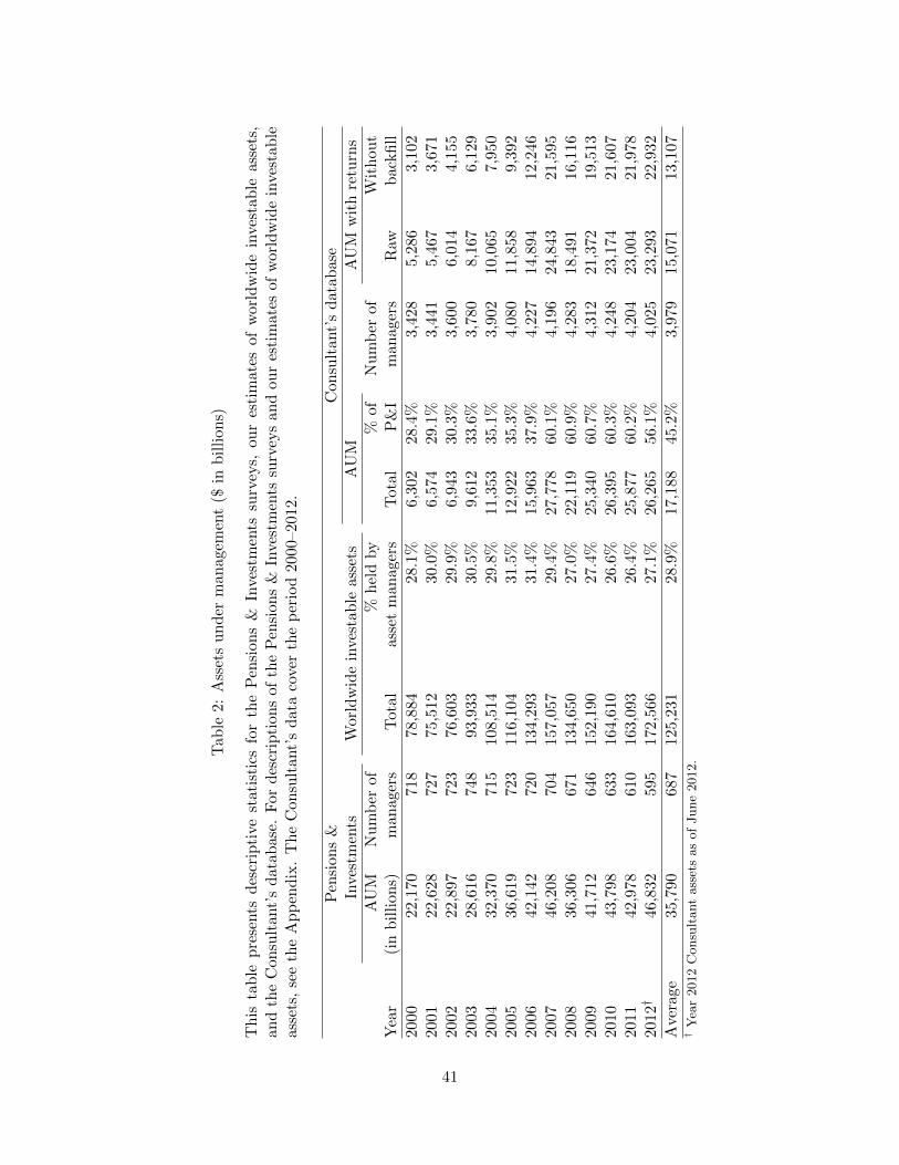
Tab
le2:
Ass
ets
un
der
man
agem
ent
($in
bil
lion
s)
Th
ista
ble
pre
sents
des
crip
tive
stat
isti
csfo
rth
eP
ensi
ons
&In
ves
tmen
tssu
rvey
s,ou
res
tim
ate
sof
wor
ldw
ide
inve
stab
leass
ets,
and
the
Con
sult
ant’
sd
ata
base
.F
ord
escr
ipti
ons
ofth
eP
ensi
ons
&In
vest
men
tssu
rvey
san
dou
res
tim
ates
of
wor
ldw
ide
inve
stab
leas
sets
,se
eth
eA
pp
end
ix.
Th
eC
on
sult
ant’
sd
ata
cove
rth
ep
erio
d20
00–2
012.
Pen
sion
s&
Con
sult
ant’
sd
atab
ase
Inve
stm
ents
Wor
ldw
ide
inve
stab
leas
sets
AU
MA
UM
wit
hre
turn
sA
UM
Nu
mb
erof
%h
eld
by
%of
Nu
mb
erof
Wit
hou
tY
ear
(in
bil
lion
s)m
anage
rsT
otal
asse
tm
anag
ers
Tot
alP
&I
manag
ers
Raw
bac
kfi
ll
2000
22,1
70
718
78,8
8428
.1%
6,30
228
.4%
3,428
5,2
86
3,1
02
2001
22,6
28
727
75,5
1230
.0%
6,57
429
.1%
3,441
5,4
67
3,6
71
2002
22,8
97
723
76,6
0329
.9%
6,94
330
.3%
3,600
6,0
14
4,1
55
2003
28,6
16
748
93,9
3330
.5%
9,61
233
.6%
3,780
8,1
67
6,1
29
2004
32,3
70
715
108,
514
29.8
%11
,353
35.1
%3,
902
10,0
65
7,9
50
2005
36,6
19
723
116,
104
31.5
%12
,922
35.3
%4,
080
11,8
58
9,3
92
2006
42,1
42
720
134,
293
31.4
%15
,963
37.9
%4,
227
14,8
94
12,2
46
2007
46,2
08
704
157,
057
29.4
%27
,778
60.1
%4,
196
24,8
43
21,5
95
2008
36,3
06
671
134,
650
27.0
%22
,119
60.9
%4,
283
18,4
91
16,1
16
2009
41,7
12
646
152,
190
27.4
%25
,340
60.7
%4,
312
21,3
72
19,5
13
2010
43,7
98
633
164,
610
26.6
%26
,395
60.3
%4,
248
23,1
74
21,6
07
2011
42,9
78
610
163,
093
26.4
%25
,877
60.2
%4,
204
23,0
04
21,9
78
2012†
46,8
3259
517
2,56
627
.1%
26,2
6556
.1%
4,0
25
23,
293
22,
932
Ave
rage
35,7
9068
712
5,23
128
.9%
17,1
8845
.2%
3,9
79
15,
071
13,
107
†Y
ear
2012
Consu
ltant
ass
ets
as
of
June
2012.
41
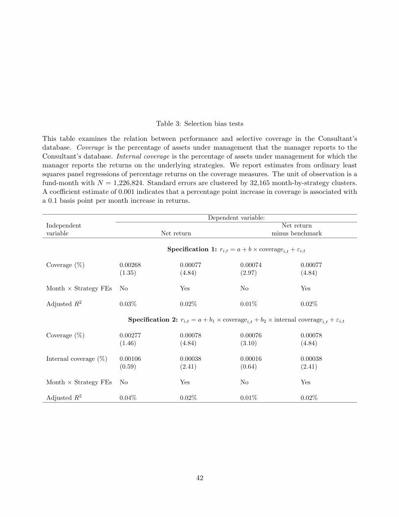
Table 3: Selection bias tests
This table examines the relation between performance and selective coverage in the Consultant’sdatabase. Coverage is the percentage of assets under management that the manager reports to theConsultant’s database. Internal coverage is the percentage of assets under management for which themanager reports the returns on the underlying strategies. We report estimates from ordinary leastsquares panel regressions of percentage returns on the coverage measures. The unit of observation is afund-month with N = 1,226,824. Standard errors are clustered by 32,165 month-by-strategy clusters.A coefficient estimate of 0.001 indicates that a percentage point increase in coverage is associated witha 0.1 basis point per month increase in returns.
Dependent variable:Independent Net returnvariable Net return minus benchmark
Specification 1: ri,t = a+ b× coveragei,t + εi,t
Coverage (%) 0.00268 0.00077 0.00074 0.00077(1.35) (4.84) (2.97) (4.84)
Month × Strategy FEs No Yes No Yes
Adjusted R2 0.03% 0.02% 0.01% 0.02%
Specification 2: ri,t = a+ b1 × coveragei,t + b2 × internal coveragei,t + εi,t
Coverage (%) 0.00277 0.00078 0.00076 0.00078(1.46) (4.84) (3.10) (4.84)
Internal coverage (%) 0.00106 0.00038 0.00016 0.00038(0.59) (2.41) (0.64) (2.41)
Month × Strategy FEs No Yes No Yes
Adjusted R2 0.04% 0.02% 0.01% 0.02%
42

Table 4: Summary of fund characteristics by asset class
This table presents descriptive statistics for the funds in the Consultant’s database. Panel A reportsthe number of managers and funds, the average fund age, and the average AUM for all funds. InPanel B, we calculate each month the distributions of assets, client counts, and AUM per client foreach fund and then report the time series averages of these distributions. Total assets and assets perclient are in $ millions. The Consultant’s data cover the period from January 2000 through June 2012.
Panel A: Number of managers and funds and average AUMNumber of Number of Average Total AUM % of
Asset class managers funds fund age per year ($M) total AUM
All 3,318 15,893 11.7 9,101,546 100%U.S. public equity 1,232 4,956 6.1 2,396,141 26%Global public equity 1,067 6,255 15.6 2,724,748 30%U.S. fixed income 586 2,206 6.0 2,219,037 24%Global fixed income 433 2,476 20.8 1,761,620 19%
Panel B: Distributions of assets, client counts, and AUM per clientPercentiles
Asset class Mean SD 25 50 75
AllAssets 1,812.4 6,918.7 108.8 410.6 1,371.7Clients 229.6 3,024.0 1.8 6.5 21.8AUM per client 293.3 1,693.8 12.6 55.3 170.2
U.S. public equityAssets 1,358.4 4,158.4 83.4 339.1 1,103.4Clients 122.3 800.0 2.5 7.8 28.0AUM per client 175.9 491.1 6.3 30.6 125.0
Global public equityAssets 1,697.5 4,488.5 107.4 407.9 1.4Clients 421.4 4,464.5 1.5 5.4 28.7AUM per client 340.2 1,669.6 15.4 61.1 164.6
U.S. fixed incomeAssets 2,598.7 9,988.3 165.7 526.5 1,965.0Clients 49.2 175.6 3.2 10.1 27.8AUM per client 198.8 445.0 20.5 74.4 217.5
Global fixed incomeAssets 2,219.1 8,964.6 152.9 501.3 1,567.4Clients 38.8 196.9 1.6 5.5 16.7AUM per client 475.2 2,278.1 45.5 131.5 272.6
43
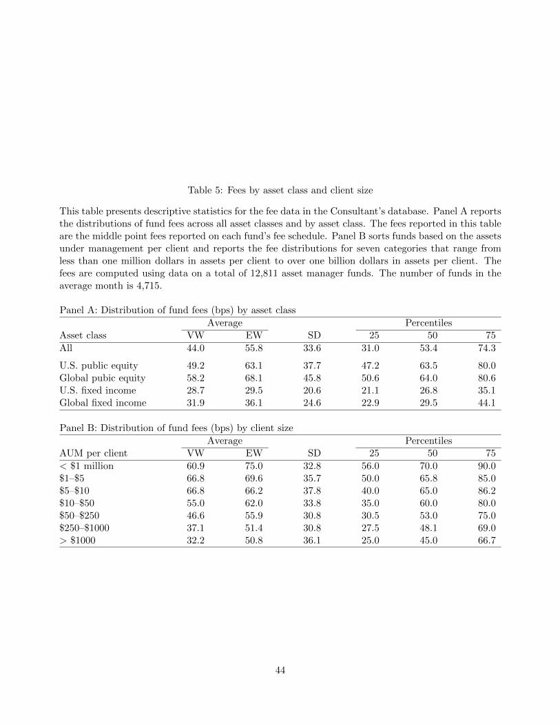
Table 5: Fees by asset class and client size
This table presents descriptive statistics for the fee data in the Consultant’s database. Panel A reportsthe distributions of fund fees across all asset classes and by asset class. The fees reported in this tableare the middle point fees reported on each fund’s fee schedule. Panel B sorts funds based on the assetsunder management per client and reports the fee distributions for seven categories that range fromless than one million dollars in assets per client to over one billion dollars in assets per client. Thefees are computed using data on a total of 12,811 asset manager funds. The number of funds in theaverage month is 4,715.
Panel A: Distribution of fund fees (bps) by asset class
Average PercentilesAsset class VW EW SD 25 50 75
All 44.0 55.8 33.6 31.0 53.4 74.3
U.S. public equity 49.2 63.1 37.7 47.2 63.5 80.0Global pubic equity 58.2 68.1 45.8 50.6 64.0 80.6U.S. fixed income 28.7 29.5 20.6 21.1 26.8 35.1Global fixed income 31.9 36.1 24.6 22.9 29.5 44.1
Panel B: Distribution of fund fees (bps) by client size
Average PercentilesAUM per client VW EW SD 25 50 75
< $1 million 60.9 75.0 32.8 56.0 70.0 90.0$1–$5 66.8 69.6 35.7 50.0 65.8 85.0$5–$10 66.8 66.2 37.8 40.0 65.0 86.2$10–$50 55.0 62.0 33.8 35.0 60.0 80.0$50–$250 46.6 55.9 30.8 30.5 53.0 75.0$250–$1000 37.1 51.4 30.8 27.5 48.1 69.0> $1000 32.2 50.8 36.1 25.0 45.0 66.7
44

Table 6: Fund returns
This table compares fund returns against broad asset-class benchmarks. Panel A reports market-adjusted returns, which are computed by subtracting from each fund’s gross or net return the broadasset-class level benchmark return. These four benchmarks are listed in Table A3. Panel B presentsthe annual gross alphas and weights against the asset-class level benchmarks. We define for eachfund i and month t a residual eit = rit − rBit , where rBit is the return on the broad asset class orstrategy. We then estimate a value-weighted panel regression of these residuals against a constant,clustering the errors by month. The weights in this regression are proportional to each fund’s assetsunder management and they are scaled to sum up to one within each month. Tracking error estimatesare obtained from value-weighted regressions of e2its on a constant. Alphas and tracking errors areannualized. Information ratio (IR) is the annualized net alpha divided by the tracking error. TheConsultant’s data cover the period from January 2000 through June 2012.
45
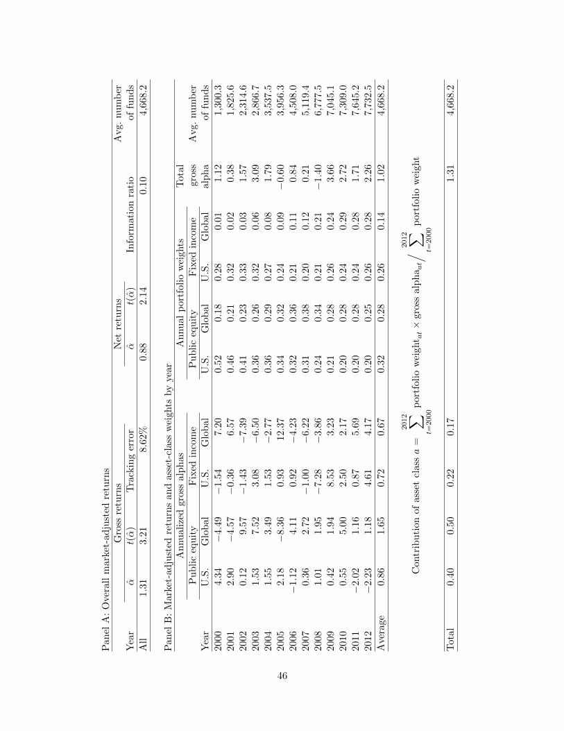
Pan
elA
:O
vera
llm
ark
et-a
dju
sted
retu
rns
Gro
ssre
turn
sN
etre
turn
sA
vg.
nu
mb
erY
ear
αt(α
)T
rack
ing
erro
rα
t(α
)In
form
atio
nra
tio
offu
nd
s
All
1.31
3.21
8.62
%0.8
82.
140.
104,
668
.2
Pan
elB
:M
ark
et-a
dju
sted
retu
rns
an
dass
et-c
lass
wei
ghts
by
year
An
nu
aliz
edgro
ssal
ph
asA
nnu
alp
ortf
olio
wei
ghts
Tota
lP
ub
lic
equ
ity
Fix
edin
com
eP
ub
lic
equ
ity
Fix
edin
com
egr
oss
Avg.
nu
mb
erY
ear
U.S
.G
lob
al
U.S
.G
lob
alU
.S.
Glo
bal
U.S
.G
lob
al
alp
ha
of
fun
ds
2000
4.3
4−
4.4
9−
1.54
7.20
0.5
20.1
80.2
80.
011.
121,3
00.
320
01
2.9
0−
4.5
7−
0.36
6.5
70.4
60.2
10.3
20.
020.
381,8
25.
620
02
0.1
29.
57−
1.43
−7.3
90.4
10.2
30.3
30.
03
1.57
2,314
.62003
1.5
37.
52
3.08
−6.5
00.3
60.2
60.3
20.
063.
092,8
66.
720
04
1.5
53.
491.
53−
2.7
70.3
60.2
90.2
70.
08
1.79
3,537
.52005
2.1
8−
8.3
60.
9312.3
70.3
40.3
20.2
40.
09
−0.
60
3,956
.32006
−1.
124.
11
0.92
−4.2
30.3
20.3
60.2
10.
110.
844,5
08.
020
07
0.3
62.
72−
1.00
−6.2
20.3
10.3
80.2
00.
12
0.21
5,119
.42008
1.0
11.
95
−7.
28
−3.8
60.2
40.3
40.2
10.
21−
1.40
6,7
77.
520
09
0.4
21.
948.
533.
230.2
10.2
80.2
60.
24
3.66
7,045
.12010
0.5
55.
00
2.50
2.17
0.2
00.2
80.2
40.
292.
727,3
09.
020
11
−2.
02
1.16
0.87
5.69
0.2
00.2
80.2
40.
28
1.71
7,645
.22012
−2.
231.
18
4.61
4.17
0.2
00.2
50.2
60.
282.
267,7
32.
5
Ave
rage
0.86
1.65
0.72
0.67
0.3
20.2
80.2
60.
14
1.02
4,668
.2
Contr
ibu
tion
of
asse
tcl
assa
=2012 ∑
t=2000
por
tfol
iow
eigh
t at×
gros
sal
ph
aat/20
12 ∑
t=2000
port
foli
ow
eight
Tota
l0.4
00.
500.
220.
171.3
14,
668
.2
46
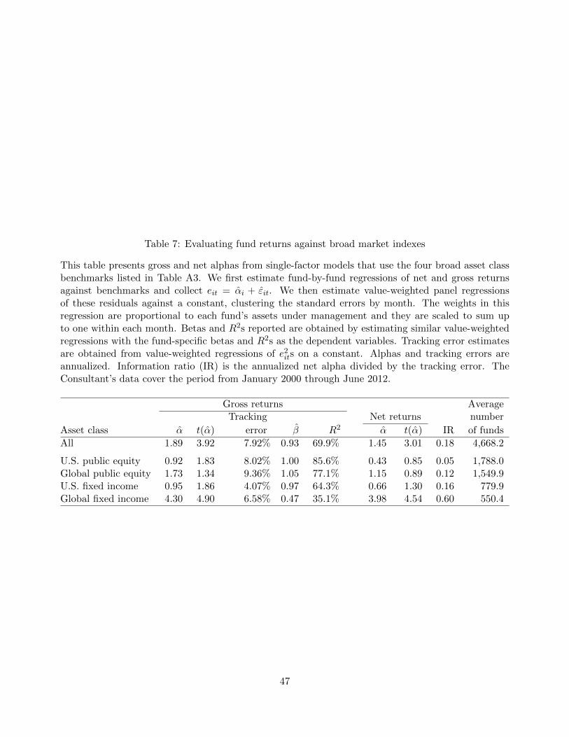
Table 7: Evaluating fund returns against broad market indexes
This table presents gross and net alphas from single-factor models that use the four broad asset classbenchmarks listed in Table A3. We first estimate fund-by-fund regressions of net and gross returnsagainst benchmarks and collect eit = αi + εit. We then estimate value-weighted panel regressionsof these residuals against a constant, clustering the standard errors by month. The weights in thisregression are proportional to each fund’s assets under management and they are scaled to sum upto one within each month. Betas and R2s reported are obtained by estimating similar value-weightedregressions with the fund-specific betas and R2s as the dependent variables. Tracking error estimatesare obtained from value-weighted regressions of e2its on a constant. Alphas and tracking errors areannualized. Information ratio (IR) is the annualized net alpha divided by the tracking error. TheConsultant’s data cover the period from January 2000 through June 2012.
Gross returns AverageTracking Net returns number
Asset class α t(α) error β R2 α t(α) IR of funds
All 1.89 3.92 7.92% 0.93 69.9% 1.45 3.01 0.18 4,668.2
U.S. public equity 0.92 1.83 8.02% 1.00 85.6% 0.43 0.85 0.05 1,788.0Global public equity 1.73 1.34 9.36% 1.05 77.1% 1.15 0.89 0.12 1,549.9U.S. fixed income 0.95 1.86 4.07% 0.97 64.3% 0.66 1.30 0.16 779.9Global fixed income 4.30 4.90 6.58% 0.47 35.1% 3.98 4.54 0.60 550.4
47

Table 8: Evaluating fund returns against strategy-specific benchmarks
This table presents gross and net alphas from single-factor models that use the 170 strategies listedin Table A5. Panel A reports the estimates by asset class. Panel B reports estimates based onalternative samples for robustness. The first row in Panel B limits the sample to funds for which themanager entered no more than one year of historical data at the initiation of coverage. The secondrow presents results for the post-2006 data and the third row limits the sample to asset managersthat report performance for funds that represent at least 85% of their total assets under management.We first estimate fund-by-fund regressions of net and gross returns against benchmarks and collecteit = αi + εit. We then estimate value-weighted panel regressions of these residuals against a constant,clustering the standard errors by month. The weights in this regression are proportional to eachfund’s assets under management and they are scaled to sum up to one within each month. Betasand R2s reported are obtained by estimating similar value-weighted regressions with the fund-specificbetas and R2s as the dependent variables. Tracking error estimates are obtained from value-weightedregressions of e2its on a constant. Alphas and tracking errors are annualized. Information ratio (IR) isthe annualized net alpha divided by the tracking error. The Consultant’s data cover the period fromJanuary 2000 through June 2012.
Panel A: Single-factor model regressions against strategy benchmarksGross returns Average
Tracking Net returns number
Asset class α t(α) error β R2 α t(α) IR of funds
All 0.86 3.35 5.62% 0.94 82.3% 0.42 1.63 0.07 4,668.2
U.S. public equity 0.39 0.97 6.25% 0.98 89.8% −0.10 −0.25 −0.02 1,788.0Global public equity 0.58 1.26 6.02% 0.96 90.3% 0.00 0.01 0.00 1,549.9U.S. fixed income 1.36 6.59 2.93% 0.84 73.5% 1.07 5.19 0.36 779.9Global fixed income 1.29 3.15 4.92% 0.95 69.2% 0.97 2.37 0.20 550.4
Panel B: RobustnessGross returns Average
Tracking Net returns number
Sample or specification α t(α) error β R2 α t(α) IR of funds
No more than one year 0.80 3.03 5.33% 0.93 83.2% 0.35 1.34 0.07 2,411.4of historical data
Only post-2006 data 0.67 1.92 5.36% 0.94 80.7% 0.23 0.67 0.04 6,503.1Strategy coverage ≥ 85% 0.74 1.76 5.74% 0.94 85.4% 0.18 0.44 0.03 436.5
48
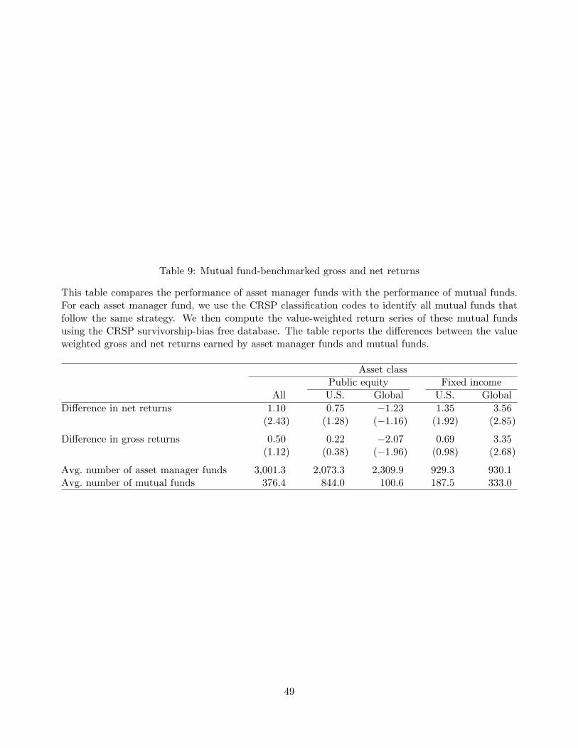
Table 9: Mutual fund-benchmarked gross and net returns
This table compares the performance of asset manager funds with the performance of mutual funds.For each asset manager fund, we use the CRSP classification codes to identify all mutual funds thatfollow the same strategy. We then compute the value-weighted return series of these mutual fundsusing the CRSP survivorship-bias free database. The table reports the differences between the valueweighted gross and net returns earned by asset manager funds and mutual funds.
Asset classPublic equity Fixed income
All U.S. Global U.S. Global
Difference in net returns 1.10 0.75 −1.23 1.35 3.56(2.43) (1.28) (−1.16) (1.92) (2.85)
Difference in gross returns 0.50 0.22 −2.07 0.69 3.35(1.12) (0.38) (−1.96) (0.98) (2.68)
Avg. number of asset manager funds 3,001.3 2,073.3 2,309.9 929.3 930.1Avg. number of mutual funds 376.4 844.0 100.6 187.5 333.0
49

Table 10: Average returns, standard deviations, and Sharpe ratios for asset manager funds, broadasset class benchmarks, and strategy-specific benchmarks
This table reports average returns, standard deviations, and Sharpe ratios for asset managers funds,the broad asset class benchmarks, and the strategy-specific benchmarks. The estimates are reportedby asset class. The return on the strategy-specific benchmark is the value-weighted average of all thestrategies within each asset class, with the weights proportional to asset manager funds’ AUMs. Thelast row examines the performance of equity and fixed income asset classes.
Asset managers Asset-class benchmark Strategy benchmarkAverage Sharpe Average Sharpe Average Sharpe
Asset class return SD ratio return SD ratio return SD ratio
U.S. public equity 4.46 16.69 0.14 3.62 16.68 0.09 4.23 16.55 0.12Global public equity 4.01 16.87 0.11 2.31 15.57 0.01 3.66 17.30 0.09U.S. fixed income 7.10 3.90 1.26 6.36 3.61 1.16 6.83 4.22 1.10Global fixed income 7.03 4.85 1.00 6.41 8.50 0.50 6.02 4.61 0.83
1-month T-bill 2.17 0.63
All 5.23 10.33 0.30 3.91 9.79 0.18 4.82 10.37 0.26
50

Table 11: Sharpe analysis
This table reports estimates from an analysis that compares fund returns with returns on mimickingportfolios constructed from 15 tactical factors. We implement this analysis using a modified versionof Sharpe’s (1992) approach. For each fund i-month t, we regress the strategy returns against 15tactical factors using data up to month t − 1. The first tactical factor is the strategy’s broad assetclass benchmark listed in Table A3. The remaining 14 tactical factors, which are listed in Panel A,are common across strategies. The regression slopes are constrained to be non-negative and to sumup to one. We use the resulting slope estimates to compute the return on strategy i’s style portfolioin month t and define a residual eit = rit − rBit , where rBit is the return on the style portfolio. We thenestimate a value-weighted panel regression of these residuals against a constant, clustering the errorsby month. The weights in this regression are proportional to each fund’s assets under managementand they are scaled to sum up to one within each month. Panel A reports the average weights byasset class. Panel B reports gross and net alphas, tracking errors, and information ratios for the fundsby asset class. The tracking error and Sharpe weight estimates are obtained from value-weightedregressions of e2its and the first-stage weights on a constant. The Consultant’s data cover the periodfrom January 2000 through June 2012.
51

Pan
elA
:S
harp
ew
eigh
ts(w
1+
···+
w15
=10
0%)
Ass
etC
lass
U.S
.G
lob
al
U.S
.G
lob
alp
ub
lic
pu
bli
cfi
xed
fixed
Fact
ors
All
equ
ity
equ
ity
inco
me
inco
me
Ass
et-c
lass
ben
chm
ark
18.7
Ru
ssel
l300
09.
9M
SC
IW
orld
exU
.S.
20.8
Bar
clay
sC
ap
ital
U.S
.A
ggre
gate
25.0
Bar
clay
sC
apit
al
Mu
ltiv
erse
exU
.S.
27.
2E
qu
ity:
US
S&
P500/
Cit
igro
up
Val
ue
10.8
28.8
3.9
0.7
0.8
S&
P50
0/C
itig
rou
pG
row
th9.2
22.8
7.4
0.5
0.6
S&
P40
0M
idca
p3.
910.9
1.9
0.6
0.4
S&
PS
mal
lC
ap6.
114.4
3.3
0.9
1.6
Equ
ity:
Glo
bal
S&
PE
uro
pe
BM
I10.1
2.1
32.2
0.7
1.2
MS
CI
Em
ergi
ng
Mar
ket
Fre
eF
loat
Ad
just
edIn
dex
6.8
3.6
18.1
1.2
1.6
FI:
US
U.S
.3
Month
T-B
ill
5.8
1.8
1.8
8.3
18.0
Barc
lays
Cap
ital
US
Inte
rmed
iate
Gov
t4.4
0.3
0.8
12.1
6.5
Barc
lays
Cap
ital
US
Lon
gG
ovt
5.2
1.0
2.5
8.3
12.1
Barc
lays
Cap
ital
US
Corp
orat
eIn
ves
tmen
tG
rad
e8.5
0.6
1.8
22.7
9.6
Barc
lays
Cap
ital
US
Mort
gag
eB
ack
edS
ecu
riti
es4.8
0.7
1.2
14.4
2.8
FI:
Glo
bal
Barc
lays
Cap
ital
Eu
roA
ggre
gate
Gov
t1.
51.
01.
50.
24.
6B
arc
lays
Cap
ital
Eu
roA
ggre
gat
eC
orp
orat
e1.3
1.1
1.4
0.4
1.9
JP
Morg
anE
MB
IG
lob
al
Div
ersi
fied
3.0
1.0
1.3
4.0
11.3
Tota
l10
0.0
100.
0100.0
100.0
100.0
Avg.
nu
mb
erof
fun
ds
4,23
5.3
1,6
34.1
1,3
91.
7715.6
493.9
52

Panel B: Excess returns over the mimicking portfolioGross returns Net returns Average
Excess t(Excess Tracking Excess t(Excess numberAsset class return return) error R2 return return) IR of funds
All −0.27 −0.77 5.76% 84.8% −0.71 −2.00 −0.12 4,235.3
U.S. public equity −0.67 −1.50 5.75% 89.9% −1.16 −2.60 −0.20 1,634.1Global public equity −1.11 −1.50 7.23% 85.6% −1.69 −2.29 −0.23 1,391.7U.S. fixed income 0.46 1.24 2.98% 71.4% 0.17 0.45 0.06 715.6Global fixed income 0.89 1.41 4.96% 60.9% 0.58 0.91 0.12 493.9
53

Table 12: Regressions of fees on style-portfolio and residual returns
This table presents regressions that measure the relation between before-fee performance and fees.The unit of observation is a month-fund pair. We report estimates from regressions of monthly fees(×100) on the return on the style portfolio and the residual return. These return-component estimatesare from Table 11’s Sharpe analysis. Panel A presents panel regressions with monthly returns. Theseregressions include month-asset class fixed effects and standard errors are clustered at the fund-level.Panel B presents cross sectional regressions with one observation per fund. We generate each fund’sobservation by first running panel regressions of style return and the residual return on month-assetclass fixed effects. The residuals from these regressions represent abnormal performance after removingvariation across asset classes and months. For each fund, we then take averages of these adjusted styleand residual returns. The Consultant’s data cover the period from January 2000 through June 2012.
Panel A: Panel regressions by asset classDependent variable: Fees
Sample set: All asset manager fund-month observations
In asset class: All Public equities Fixed incomeU.S. Global U.S. Global
Style portfolio return 6.01 10.34 5.02 1.02 2.71(5.51) (4.32) (3.69) (0.64) (1.30)
Residual return 1.34 1.34 1.04 3.09 2.78(2.67) (1.13) (2.45) (2.52) (2.34)
Month-asset class FEs Yes Yes Yes Yes YesN 619,703 232,894 202,734 104,747 79,328Adjusted R2 0.2% 0.3% 0.1% 0.1% 0.1%
Panel B: Cross-sectional regressions by asset classDependent variable: Fees
Sample set: Asset manager fund
In asset class: All Public equities Fixed incomeU.S. Global U.S. Global
Style portfolio return 0.51 1.18 0.35 −0.05 0.29(2.83) (3.03) (1.39) (−0.18) (0.75)
Residual return −0.02 0.07 −0.15 0.03 0.44(0.35) (0.61) (−1.14) (0.48) (1.64)
Month-asset class FEs 619,703 232,894 202,734 104,747 79,328N 9,665 3,409 3,395 1,513 1,348Adjusted R2 0.6% 2.3% 0.3% -0.1% 0.7%
54

Table 13: Replicating asset managers
This table reports Sharpe ratios of alternative portfolios constructed from tradeable indexes listedin Table 7. The first method uses the standard mean-variance optimization algorithm of Markowitz(1952). The second method first diagonalizes the covariance matrix and constrains the estimatedrisk premiums to be nonnegative. The third method imposes short-sale constraints. We estimatethe means and covariances using all available historical data for each index up to month t − 1. Weconstruct the replicating portfolio separately within each asset class, and then use these weightstogether with the asset-class weights observed in the asset-manager data to compute the return onthe replicating portfolio in month t. Panel A reports the Sharpe ratios of asset managers and thesereplicating portfolios. Column Indifference cost equates the Sharpe ratio of the replicating portfoliowith the asset managers’ Sharpe ratio. Panel B reports the cost of holding the replicating portfolio,constructed using the diagonal-covariance method, using four alternative assumptions about fees. Thedetailed fees are reported in Panel C. Expense ratios and fees are reported in basis points. Entries of“NA” denote that the data are not available.
Panel A: Sharpe ratios and indifference costs of replicating portfoliosAverage Sharpe Indifference
return SD ratio cost (bps)
Asset managersGross return 5.23% 10.38% 0.295Net return 4.79% 10.38% 0.252
Replicating portfolio, gross returnStandard MV portfolio 4.42% 14.49% 0.155 −202.3MV portfolio with diagonal covariance matrix 6.43% 11.55% 0.369 85.5MV portfolio with short-sale constraints 6.16% 11.71% 0.341 53.6
Panel B: Cost (bps) of investing the replicating portfolio using the actual fees of the vehicle over theperiodVehicle Fee
Institutional mutual fundsQuartile 1 66.1Median 88.5Quartile 3 112.4
End-of-sample ETFs 24.0
55

Pan
elC
:F
ees
use
din
the
rep
lica
tin
gp
ortf
olio
sE
TF
sIn
stit
uti
on
al
Fee
Exp
ense
Sta
rtm
utu
alfu
nd
su
sed
inB
ench
mar
kra
tio
Tic
ker
dat
eQ
1M
edia
nQ
3re
pli
cati
on
S&
P500
/C
itig
rou
pV
alu
e15
SP
YV
9/29
/00
7091
112
91
S&
P500
/C
itig
rou
pG
row
th15
SP
YG
9/29
/00
80
9712
297
S&
P400
Mid
cap
15IV
OO
9/9/
1070
95115
.595
S&
PS
mall
Cap
15S
LY
11/1
5/05
85109
135
109
S&
PE
uro
pe
BM
I12
VG
K3/
10/0
554.
588
129
88M
SC
IE
mer
gin
gM
ark
etF
ree
Flo
atA
dju
sted
67E
EM
4/11
/03
102
139
166
139
U.S
.3
Month
T-B
ill
14B
IL5/
30/0
716
2645
26B
arcl
ays
Cap
ital
US
Inte
rmed
iate
Gov
t20
GV
I1/
5/07
51
6683
66B
arcl
ays
Cap
ital
US
Lon
gG
ovt
12V
GLT
11/2
4/09
20
43
6743
Bar
clay
sC
apit
al
US
Cor
pora
teIn
ves
tmen
tG
rad
e15
LQ
D7/
26/0
255
7092
70
Bar
clay
sC
apit
al
US
Mor
tgage
Bac
ked
Sec
uri
ties
32M
BG
1/15
/09
4965
80
65
Bar
clay
sC
apit
al
Eu
roA
ggr
egate
Gov
15G
OV
Y5/
23/1
1N
AN
AN
A15
Bar
clay
sC
apit
al
Eu
roA
ggr
egate
Corp
orat
e20
IBC
X3/
17/0
3N
AN
AN
A20
JP
Mor
gan
EM
BI
Glo
bal
Div
ersi
fied
40E
MB
12/1
9/07
84
97
112
97
56

Table 14: Evaluating theories of delegation
This table reports estimates from regressions that explain variation in gross and net alphas and feeswith manager size, average client size, fees, and price inefficiency. Manager size is the manager’s totalassets under management. We compute each manager’s total size each month and define *managersize* as the manager’s percentile rank in the cross-sectional distribution. Average client size is themanager’s total assets divided by the number of clients. We define *average client size* as the man-ager’s percentile rank in the cross-sectional distribution. Fee is the reported fee from the fee schedule.For managers with multiple fee tiers, we use the fee associated with the median tier. Price inefficiencyis defined as the strategy level as the variance of the gross return of the average dollar in the strategyscaled by the variance of the gross return of the average dollar in the asset class. We define *priceinefficiency* as the percentile rank of a strategy’s price inefficiency measure. In Panel A we reportestimates from panel regressions in which the unit of observation is a fund-month pair. We estimateregressions with either asset class-month or strategy-month fixed effects and cluster standard errorsby month. We only include those observations in the manager reports performance on gross or netbasis. That is, we do not use fee information to infer gross returns from net returns, or vice versa. InPanel B we report estimates from cross-sectional regressions in which the unit of observation is a fund.The dependent variable is the reported fee at the end of the sample (or when the fund disappears) andthe explanatory variables are the time-series averages of the predictors described above. The sampleperiod is from January 2000 through December 2012.
Panel A: Gross and net returnsGross returns Net returns
Regressor (1) (2) (3) (4)
Manager size −10.04 −9.28 −23.07 −13.58(−3.24) (−3.41) (−2.44) (−1.67)
Avg. client size 6.05 4.20 8.56 4.03(1.96) (1.85) (1.46) (0.62)
Fee 0.22 0.10 0.17 0.08(2.36) (2.98) (1.36) (0.93)
Price inefficiency 41.54 37.40(1.74) (1.51)
Fixed effects Asset class × Strategy × Asset class × Strategy ×Month Month Month Month
N 601,918 601,918 49,277 49,277Adjusted R2 74.9% 87.3% 78.1% 89.7%
57

Panel B: FeesReported fee
Regressor (1) (2)
Manager size −23.32 −16.09(−16.10) (−12.20)
Avg. client size −9.72 −6.72(−6.98) (−5.33)
Price inefficiency 34.38(28.46)
Fixed effects Asset class × Strategy ×Month Month
N 9,746 9,746Adjusted R2 30.4% 44.8%
58

Appendix
In this Appendix, we describe the methodology that we use to estimate worldwide investable assetsand total institutional assets held by asset managers.
Worldwide investable assets
We estimate total worldwide investable assets, which represent the sum of six broad investable assetclasses: real estate, outstanding government bonds, outstanding bonds issued by banks and financialcorporations, outstanding bonds issued by non-financial corporations, private equity, and public equity.
For real estate, we estimate the worldwide value of commercial real estate. To do so, we followthe methodology used by Prudential Real Estate Investors (PREI) in the report “A Bird’s Eye Viewof Global Real Estate Markets: 2010 Update.” Their methodology uses GDP per capita to capturecountry-level economic development and estimates the size of a country’s commercial real estate marketbased on GDP. They select a time-varying threshold and assume that the value of commercial realestate above this threshold is 45% of total GDP. The threshold starts in 2000 at $20,000 in per capitaGDP and then adjusts annually by the U.S. inflation rate. For countries with per capita GDP belowthe threshold in a given year, PREI calculates the value of the country’s commercial real estate marketas:
Value of commercial real estate = 45% × GDP × (GDP per capita / Threshold)1/3.
To estimate the worldwide size of the government, financial, and corporate bond sectors, we usethe Bank for International Settlements’ debt securities statistics provided in Table 18 of the Bank’sQuarterly Reviews. These statistics present total debt securities by both residence of issuer andclassification of user (non-financial corporations, general government, and financial corporations).1 Wethen aggregate the country-level data by year. For private equity, we use Preqin’s “2014 Private EquityPerformance Monitor Report,” which provides annual estimates of assets under management held byprivate equity funds worldwide and these estimates include both cash held by funds (“dry powder”)and unrealized portfolio values. For our estimates of the size of world’s public equity markets, we usethe World Bank’s estimates of the market capitalization of listed companies.2
Table A1 presents annual estimates of worldwide investable assets by the six broad asset classes.Our estimate of worldwide investable assets for 2012 is $173 trillion. For comparison, if we extrapolatePhilippon’s (2015) estimates of U.S. investable assets, we obtain a similar estimate of $175 trillion inworldwide investable assets for 2012.
Total institutional assets held by asset managers
In our analysis, we supplement the Consultant’s database with data from Pensions & InvestmentsMagazine, which implements annual surveys of the asset management industry. In this subsection, wedescribe the Pensions & Investments surveys and how we use the surveys to construct our estimates oftotal institutional assets under management held worldwide by asset managers, which are presentedin the first column of Panel A of Table 2.
We use two Pensions & Investments surveys. The first survey is the Pensions & InvestmentsTowers Watson World 500, which is an annual survey of the assets under management (retail and
1The data are available at https://www.bis.org/statistics/hanx18.csv.2The data are available at http://data.worldbank.org/indicator/CM.MKT.LCAP.CD.
59

institutional) held by the world’s 500 largest money managers. The second survey is the Pensions& Investments Money Manager Directory, which provides more detailed data for U.S. based moneymanagers including total assets under management, institutional assets under management, and broadasset allocations (equity, fixed income, cash, and other) for U.S. tax exempt institutional assets.
Table A2 provides descriptive statistics for these surveys and describes how we construct our es-timate of total worldwide institutional assets held by asset managers. Column (1) presents annualtotal worldwide assets under management (retail and institutional assets) based on the Pensions &Investments Towers Watson World 500 survey and column (2) presents total assets under manage-ment (retail and institutional assets) for the U.S. based asset managers covered in the Pensions &Investments Money Manager Directory survey. The totals presented in these two columns includeboth retail and institutional assets. In column (3), we therefore present total institutional assets heldby U.S. based asset managers. As shown in column (4), over the sample period, institutional assetsheld by U.S. based asset managers range from 63% to 69% of total assets.
To estimate the worldwide size of the institutional segment, we extrapolate based on the institu-tional asset percentages for the U.S. based asset managers. We first create a union of managers whoshow up on either the Pensions & Investments Towers Watson 500 survey or the Pensions & Invest-ments Money Manager Directory survey.3 Column (5) presents total assets under management (retailand institutional) for the managers in the union of the two surveys. These totals are very close to thetotals based on the Towers Watson 500 survey, implying that the top 500 managers control the vastmajority of assets. We next scale the total assets presented in column (5) by the percent institutionalassets held by U.S. based managers presented in column (4). Column (6) presents these estimates ofworldwide institutional assets under management. We present these estimates in the first column ofPanel A of Table 2.
3Missing in this union are non-U.S. based asset managers who are smaller than the cutoff for the Pensions & In-vestments Towers Watson World 500. Given the close estimates of the top 500 with the intersection with U.S. basedmanagers, this missing category does not appear large.
60

Tab
leA
1:E
stim
ates
ofw
orld
wid
ein
vest
able
asse
ts($
inb
illi
ons)
Th
ista
ble
pre
sents
an
nu
al
esti
mate
sof
wor
ldw
ide
inve
stab
leas
sets
by
asse
tcl
ass
and
inag
greg
ate.
We
use
the
foll
owin
gso
urc
esto
esti
mate
the
worl
dw
ide
inve
stab
leas
sets
by
asse
tcl
ass:
real
esta
te,
Pru
den
tial
Rea
lE
stat
eIn
vest
ors;
gove
rnm
ent
bon
ds,
the
Ban
kfo
rIn
tern
ati
on
alS
ettl
emen
ts;
corp
orat
eb
ond
s,th
eB
ank
for
Inte
rnat
ion
alS
ettl
emen
ts;
pri
vate
equ
ity,
Pre
qin
;p
ub
lic
equ
ity,
the
Wor
ldB
an
k.
Yea
rR
eal
esta
teG
ovt.
bon
ds
Fin
anci
alb
ond
sC
orp
orat
eb
ond
sP
riva
teeq
uit
yP
ub
lic
equ
ity
Tot
al
200
013
,249
13,5
78
14,6
134,
788
716
31,9
4078
,884
200
113
,085
13,2
10
15,9
274,
924
751
27,6
1475
,512
200
213
,625
15,3
61
18,3
865,
216
767
23,2
4876
,603
200
315
,373
18,6
86
21,8
085,
540
870
31,6
5793
,933
200
417
,312
21,7
50
25,0
915,
727
963
37,6
7110
8,51
4200
518
,641
21,2
05
26,9
135,
413
1,23
842
,694
116,
104
200
620
,100
22,6
00
31,4
265,
801
1,70
452
,663
134,
293
200
722
,667
24,8
52
37,0
776,
437
2,27
663
,748
157,
057
200
824
,770
28,0
55
38,2
986,
757
2,27
934
,491
134,
650
200
923
,104
32,1
87
40,1
997,
535
2,48
046
,685
152,
190
201
025
,251
36,6
86
38,4
348,
102
2,77
653
,361
164,
610
201
128
,005
39,7
45
37,8
668,
565
3,03
645
,876
163,
093
201
228
,481
41,1
81
37,7
999,
380
3,27
352
,452
172,
566
61

Tab
leA
2:T
otal
inst
itu
tion
alas
sets
hel
dby
asse
tm
anag
ers
($in
mil
lion
s)
Th
ista
ble
pre
sents
how
we
esti
mat
eto
tal
inst
itu
tion
alas
sets
hel
dby
asse
tm
anag
ers.
To
do
so,
we
use
two
Pen
sion
s&
Inve
stm
ents
surv
eys:
Tow
ers
Wat
son
and
the
Mon
eyM
anag
erD
irec
tory
.T
ower
sW
atso
np
rovid
esth
eto
tal
asse
tsu
nder
man
agem
ent
(ret
ail
and
inst
itu
tion
al)
hel
dby
the
wor
ld’s
500
larg
est
asse
tm
anag
ers,
wh
ich
are
pre
sente
din
the
firs
tco
lum
n.
Th
eM
oney
Man
ager
Dir
ecto
ryp
rovid
esto
tal
ass
ets
un
der
man
agem
ent
(ret
ail
and
inst
itu
tion
al)
and
inst
itu
tion
alas
sets
un
der
man
agem
ent
for
U.S
.as
set
man
ager
s,w
hic
har
ep
rese
nte
din
the
seco
nd
and
thir
dco
lum
ns.
We
crea
tea
un
ion
ofth
ese
two
surv
eys
and
then
use
the
rati
oin
stit
uti
onal
toto
tal
ass
ets
for
U.S
.as
set
man
ager
sto
extr
apola
teto
tal
wor
ldw
ide
inst
itu
tion
alas
sets
hel
dby
asse
tm
anag
ers,
wh
ich
isp
rese
nte
din
the
last
colu
mn
.
Tow
ers
Wats
on
Mon
eyM
anag
erD
irec
tory
Un
ion
Tota
lA
UM
Tota
lA
UM
Inst
itu
tion
alA
UM
Inst
itu
tion
al%
Tot
alA
UM
Inst
itu
tion
alA
UM
200
034,
590,2
84
20,1
92,3
5412
,805
,136
63%
34,9
59,2
5222
,169
,678
200
134,
683,5
88
20,8
96,2
0413
,481
,972
65%
35,0
72,3
5222
,628
,247
200
235,
002,0
40
20,3
71,5
8813
,192
,112
65%
35,3
57,8
7622
,896
,843
200
342,
461,2
88
24,9
65,2
6016
,622
,492
67%
42,9
78,7
5228
,616
,324
200
448,
183,5
48
28,7
26,4
3619
,072
,168
66%
48,7
54,8
8032
,369
,531
200
552,
964,4
00
31,7
01,5
6421
,643
,876
68%
53,6
35,8
0036
,619
,222
200
662,
902,8
88
37,3
44,5
6424
,708
,774
66%
63,6
93,4
1642
,142
,311
200
768,
731,1
20
41,6
45,2
0427
,621
,568
66%
69,6
67,8
7246
,207
,863
200
852,
581,8
56
31,4
14,8
0021
,459
,676
68%
53,1
47,6
9236
,305
,571
200
961,
149,8
20
37,9
57,5
5625
,607
,218
67%
61,8
29,8
8441
,712
,151
201
063,
811,2
04
43,0
89,0
4329
,233
,620
68%
64,5
56,9
0443
,798
,420
201
162,
170,7
00
42,5
91,7
9729
,157
,459
68%
62,7
80,4
2042
,978
,170
201
267,
223,0
72
46,7
57,5
4232
,237
,746
69%
67,9
25,1
2846
,832
,082
62

Tab
leA
3:
Bro
ad
asse
tcl
asse
sin
the
Con
sult
ant’
sd
atab
ase
and
thei
rb
ench
mar
ks
Th
ista
ble
pre
sents
the
an
nu
al
aver
age
retu
rns
and
stan
dar
dd
evia
tion
ofre
turn
sfo
rb
oth
the
asse
tm
anag
erfu
nd
sin
the
fou
rb
road
ass
etcl
asse
san
dth
eb
ench
mark
su
sed
inT
able
6to
eval
uat
efu
nd
sp
erfo
rman
ce.
Con
sult
ant’
sd
ata
base
Ave
rage
Ben
chm
ark
Ass
etcl
ass
retu
rnS
DN
am
eR
etu
rnS
DU
.S.
pu
bli
ceq
uit
y4.
4616.6
9R
uss
ell
3000
3.2
916.6
6G
lob
alp
ub
lic
equit
y4.
0116.8
7M
SC
IW
orl
dex
U.S
.2.0
315.5
5U
.S.
fixed
inco
me
7.10
3.9
0B
arc
lays
Cap
ital
U.S
.A
ggre
gate
6.2
93.6
0G
lob
alfi
xed
inco
me
7.03
4.8
5B
arc
lays
Cap
ital
Mu
ltiv
erse
exU
.S.
6.3
68.6
1
63

Table A4: Sharpe analysis: Alternative specifications
This table reports estimates from an analysis that compares fund returns with returns on mimickingportfolios constructed from 15 tactical factors. In Table 11, we construct the style portfolio by usingdata for all months except month t. Panel A in this table constructs the style portfolio using datathat exclude six months both before and after month t. Panel B constructs the style portfolio usingdata only up to month t−1. We report gross and net alphas, tracking errors, and information ratiosfor the funds by asset class.
Panel A: Exclude month-t return observation (jackknife)Gross returns Net returns Average
Excess t(Excess Tracking Excess t(Excess numberAsset class return return) error R2 return return) IR of funds
All −0.28 −0.86 6.25% 83.4% −0.72 −2.19 −0.12 4,598.9
U.S. public equity −0.66 −1.66 6.63% 87.6% −1.15 −2.90 −0.17 1,765.3Global public equity −1.28 −1.78 7.41% 84.9% −1.86 −2.59 −0.25 1,524.8U.S. fixed income 0.55 1.67 2.93% 72.7% 0.26 0.79 0.09 767.7Global fixed income 1.01 1.73 4.83% 63.0% 0.69 1.18 0.14 541.1
Panel B: Exclude return observations in window [t− 6, t+ 6]Gross returns Net returns Average
Excess t(Excess Tracking Excess t(Excess numberAsset class return return) error R2 return return) IR of funds
All −0.31 −0.97 6.43% 82.4% −0.75 −2.35 −0.12 4,419.3
U.S. public equity −0.70 −1.83 6.89% 86.5% −1.20 −3.11 −0.17 1,711.9Global public equity −1.36 −1.86 7.51% 84.5% −1.94 −2.65 −0.26 1,451.5U.S. fixed income 0.59 1.75 2.94% 72.2% 0.30 0.89 0.10 743.9Global fixed income 1.12 1.87 4.91% 62.5% 0.81 1.34 0.16 512.0
64

Internet Appendix
This Appendix includes a table that lists the investment strategies included in the Consultant’sdatabase along with the number of funds in each strategy, the average return of the funds in thestrategy, the strategy’s benchmark, and the average return on the strategy’s benchmark.
65
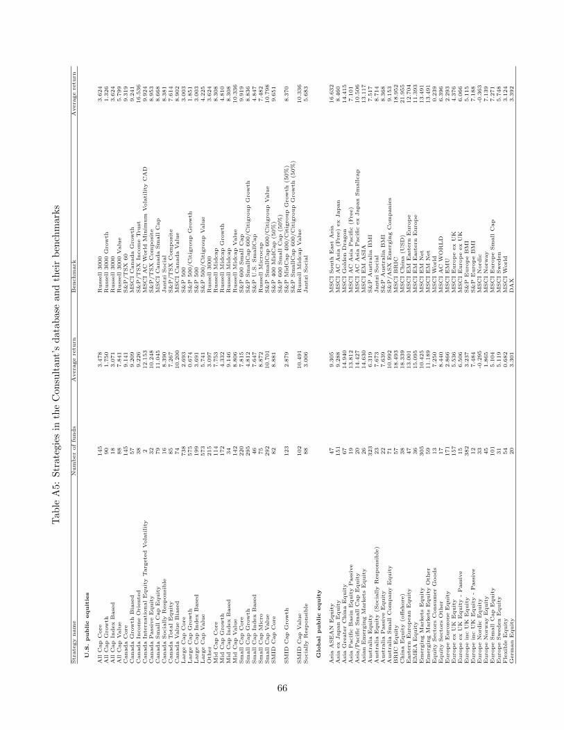
Tab
leA
5:
Str
ateg
ies
inth
eC
onsu
ltan
t’s
dat
abas
ean
dth
eir
ben
chm
arks
Str
ate
gy
nam
eN
um
ber
of
funds
Avera
ge
retu
rnB
enchm
ark
Avera
ge
retu
rn
U.S
.publi
cequit
ies
All
Cap
Core
145
3.4
78
Russ
ell
3000
3.6
24
All
Cap
Gro
wth
90
1.7
50
Russ
ell
3000
Gro
wth
1.3
26
All
Cap
Index
Base
d18
3.0
71
Russ
ell
3000
3.6
24
All
Cap
Valu
e88
7.8
41
Russ
ell
3000
Valu
e5.7
99
Canada
Core
145
9.1
41
S&
P/T
SX
60
9.3
19
Canada
Gro
wth
Bia
sed
57
9.2
09
MSC
IC
anada
Gro
wth
9.2
41
Canada
Incom
eO
riente
d38
9.2
26
S&
P/T
SX
Incom
eT
rust
16.5
36
Canada
Inte
rnati
onal
Equit
yT
arg
ete
dV
ola
tili
ty2
12.1
53
MSC
IA
CW
orl
dM
inim
um
Vola
tility
CA
D9.9
24
Canada
Pass
ive
Equit
y32
10.2
48
S&
P/T
SX
Com
posi
te8.9
53
Canada
Sm
all
Cap
Equit
y79
11.0
45
MSC
IC
anada
Sm
all
Cap
8.6
68
Canada
Socia
lly
Resp
onsi
ble
16
8.3
90
Jantz
iSocia
l8.3
81
Canada
Tota
lE
quit
y85
7.2
67
S&
P/T
SX
Com
posi
te7.6
14
Canada
Valu
eB
iase
d74
10.2
00
MSC
IC
anada
Valu
e8.9
02
Larg
eC
ap
Core
738
2.6
93
S&
P500
3.0
03
Larg
eC
ap
Gro
wth
575
0.6
74
S&
P500/C
itig
roup
Gro
wth
1.8
51
Larg
eC
ap
Index
Base
d199
3.6
91
S&
P500
3.0
03
Larg
eC
ap
Valu
e573
5.7
41
S&
P500/C
itig
roup
Valu
e4.2
25
Oth
er
215
3.0
97
Russ
ell
3000
3.6
24
Mid
Cap
Core
114
7.7
53
Russ
ell
Mid
cap
8.3
08
Mid
Cap
Gro
wth
172
4.3
32
Russ
ell
Mid
cap
Gro
wth
4.8
10
Mid
Cap
Index
Base
d34
9.1
46
Russ
ell
Mid
cap
8.3
08
Mid
Cap
Valu
e142
8.8
06
Russ
ell
Mid
cap
Valu
e10.3
36
Sm
all
Cap
Core
220
7.8
15
S&
P600
Sm
all
Cap
9.9
19
Sm
all
Cap
Gro
wth
295
4.8
12
S&
PSm
allC
ap
600/C
itig
roup
Gro
wth
8.8
36
Sm
all
Cap
Index
Base
d46
7.6
47
S&
PU
.S.
Sm
allC
ap
4.8
47
Sm
all
Cap
Mic
ro75
8.8
72
Russ
ell
Mic
rocap
7.4
82
Sm
all
Cap
Valu
e292
10.7
01
S&
PSm
allC
ap
600/C
itig
roup
Valu
e10.7
98
SM
IDC
ap
Core
82
8.8
81
S&
P400
Mid
Cap
(50%
)9.6
51
S&
P600
Sm
all
Cap
(50%
)SM
IDC
ap
Gro
wth
123
2.8
79
S&
PM
idC
ap
400/C
itig
roup
Gro
wth
(50%
)8.3
70
S&
PSm
allC
ap
600/C
itig
roup
Gro
wth
(50%
)SM
IDC
ap
Valu
e102
10.4
91
Russ
ell
Mid
cap
Valu
e10.3
36
Socia
lly
Resp
onsi
ble
88
3.0
06
Jantz
iSocia
l5.6
83
Glo
bal
publi
cequit
y
Asi
aA
SE
AN
Equit
y47
9.3
05
MSC
ISouth
East
Asi
a16.6
32
Asi
aex
Japan
Equit
y151
9.2
88
MSC
IA
CA
sia
(Fre
e)
ex
Japan
8.4
60
Asi
aG
reate
rC
hin
aE
quit
y67
14.9
40
MSC
IG
old
en
Dra
gon
14.4
15
Asi
aP
acifi
cB
asi
nE
quit
yP
ass
ive
19
13.8
12
MSC
IA
CA
sia
Pacifi
c(F
ree)
7.1
01
Asi
a/P
acifi
cSm
all
Cap
Equit
y20
14.4
27
MSC
IA
CA
sia
Pacifi
cex
Japan
Sm
allcap
10.5
06
Asi
an
Em
erg
ing
Mark
ets
Equit
y26
14.6
30
MSC
IE
MA
SIA
13.1
17
Aust
ralia
Equit
y323
6.3
19
S&
PA
ust
ralia
BM
I7.5
17
Aust
ralia
Equit
y(S
ocia
lly
Resp
onsi
ble
)23
7.6
73
Jantz
iSocia
l8.7
14
Aust
ralia
Pass
ive
Equit
y22
7.6
39
S&
PA
ust
ralia
BM
I8.3
68
Aust
ralia
Sm
all
Com
pany
Equit
y71
10.9
92
S&
P/A
SX
Em
erg
ing
Com
panie
s9.1
53
BR
ICE
quit
y57
18.4
93
MSC
IB
RIC
18.9
52
Chin
aE
quit
y(o
ffsh
ore
)38
18.3
39
MSC
IC
hin
a(U
SD
)21.9
55
East
ern
Euro
pean
Equit
y47
13.0
01
MSC
IE
ME
ast
ern
Euro
pe
12.7
04
EM
EA
Equit
y36
15.0
95
MSC
IE
ME
ast
ern
Euro
pe
11.3
93
Em
erg
ing
Mark
ets
Equit
y305
10.4
25
MSC
IE
MN
et
13.4
91
Em
erg
ing
Mark
ets
Equit
yO
ther
59
11.1
89
MSC
IE
MN
et
13.4
91
Equit
ySecto
rsC
onsu
mer
Goods
13
7.2
50
MSC
IW
orl
d0.2
39
Equit
ySecto
rsO
ther
17
8.4
40
MSC
IA
CW
OR
LD
6.3
96
Euro
pe
Euro
zone
Equit
y171
2.8
66
MSC
IE
MU
2.2
93
Euro
pe
ex
UK
Equit
y157
5.5
36
MSC
IE
uro
pe
ex
UK
4.3
76
Euro
pe
ex
UK
Equit
y-
Pass
ive
15
6.5
06
MSC
IE
uro
pe
ex
UK
6.0
66
Euro
pe
inc
UK
Equit
y382
3.2
37
S&
PE
uro
pe
BM
I5.1
15
Euro
pe
inc
UK
Equit
y-
Pass
ive
12
7.4
84
S&
PE
uro
pe
BM
I7.1
88
Euro
pe
Nord
icE
quit
y33
-0.2
95
MSC
IN
ord
ic-0
.363
Euro
pe
Norw
ay
Equit
y45
1.8
65
MSC
IN
orw
ay
7.1
39
Euro
pe
Sm
all
Cap
Equit
y101
5.1
04
MSC
IE
uro
pe
Sm
all
Cap
7.2
71
Euro
pe
Sw
eden
Equit
y31
5.1
19
MSC
ISw
eden
5.7
48
Fle
xib
leE
quit
y54
0.6
82
MSC
IW
orl
d3.1
24
Germ
an
Equit
y20
3.3
01
DA
X3.3
92
66

Str
ate
gy
nam
eN
um
ber
of
funds
Avera
ge
retu
rnB
enchm
ark
Avera
ge
retu
rn
Glo
bal
Equit
y-
Core
631
2.1
62
MSC
IW
orl
d3.1
24
Glo
bal
Equit
y-
Gro
wth
152
0.7
99
MSC
IW
orl
dG
row
th1.5
11
Glo
bal
Equit
y-
Pass
ive
76
0.4
85
MSC
IW
orl
d4.6
20
Glo
bal
Equit
y-
Valu
e204
5.4
72
MSC
IW
orl
dV
alu
e4.6
42
Glo
bal
Sm
all
Cap
Equit
y57
4.2
98
MSC
IW
orl
dSm
all
Cap
Index
7.2
41
Gold
&P
recio
us
Meta
ls15
26.1
60
S&
PG
SC
IP
recio
us
Meta
lsT
ota
lR
etu
rn18.6
62
Healt
h/B
iote
ch
23
7.0
69
S&
PH
ealt
hcare
Equip
.Sel
11.0
58
HK
OR
SO
58
4.3
42
Hang
Seng
TR
Index
14.8
95
Hong
Kong
Equit
y34
16.2
41
FT
SE
MP
FH
ong
Kong
13.8
80
India
nE
quit
y54
18.6
32
MSC
IIn
dia
19.3
57
Inte
rnati
onal
Equit
yG
lobal
Equit
ySust
ain
abilit
y7
13.4
33
MSC
IE
M1.3
07
Inte
rnati
onal
Equit
yG
lobal
Equit
ySust
ain
abilit
y167
4.1
77
MSC
IW
orl
dE
SG
-0.7
90
Inte
rnati
onal
Equit
yG
lobal
Equit
ySust
ain
abilit
y4
3.2
73
MSC
IW
orl
dE
SG
13.1
84
Inte
rnati
onal
Equit
yT
arg
ete
dV
ola
tility
20
4.0
19
MSC
IW
orl
dM
inim
um
Vola
tility
5.1
28
Inte
rnati
onal
Equit
yW
orl
dex
Japan
Equit
y116
2.1
63
MSC
IW
orl
d5.0
78
Japan
Equit
y417
-2.2
03
MSC
IJapan
-0.7
76
Japan
Pass
ive
Equit
y28
1.5
58
MSC
IJapan
4.0
33
Japan
Sm
all
Cap
Equit
y55
3.9
18
MSC
IK
okusa
iA
llC
ap
0.5
06
Kore
aE
quit
y23
7.1
65
MSC
IK
ore
a10.5
15
Lati
nA
meri
can
Equit
y40
14.9
14
MSC
IL
ati
nA
meri
ca
17.0
01
Mix
ed
UK
/N
on-U
KE
quit
y27
7.1
11
FT
SE
All
Share
3.4
12
Natu
ral
Reso
urc
es
45
13.3
64
S&
PG
lobal
Natu
ral
Reso
urc
es
SK
-8.9
28
New
Zeala
nd
Equit
y46
8.4
66
NZ
X50
(40
pri
or
to1
Oct
2003)
7.2
23
Oth
er
75
3.7
33
MSC
IW
orl
d3.1
24
Pacifi
cB
asi
nex
Japan
Equit
y149
9.5
82
MSC
IP
acifi
cex
Japan
10.7
36
Pacifi
cB
asi
nin
cJapan
Equit
y85
3.4
06
MSC
IP
acifi
c2.1
06
Sin
gap
ore
Equit
y17
9.9
95
MSC
ISin
gap
ore
10.6
76
Sw
iss
Equit
y67
7.0
61
MSC
ISw
itzerl
and
6.8
86
Technolo
gy
24
0.6
02
MSC
IA
CW
orl
d:
Secto
r:In
form
ati
on
Technolo
gy
-1.1
76
UK
All
Cap
309
4.2
48
MSC
IU
K3.9
71
UK
Pass
ive
Equit
y44
5.2
92
MSC
IU
K4.6
10
UK
Sm
all
Cap
50
8.0
59
Hoare
Govett
Sm
aller
Com
panie
s7.9
54
UK
Socia
lly
Resp
onsi
ble
15
4.2
35
MSC
IW
orl
dE
SG
-0.7
90
Worl
dex
US/E
AF
EE
quit
y-
Core
341
2.7
59
MSC
IE
AF
E3.4
25
Worl
dex
US/E
AF
EE
quit
y-
Gro
wth
142
1.8
73
MSC
IE
AF
EG
row
th1.6
29
Worl
dex
US/E
AF
EE
quit
y-
Pass
ive
52
3.3
84
MSC
IE
AF
E3.4
25
Worl
dex
US/E
AF
EE
quit
y-
Valu
e146
6.7
57
MSC
IE
AF
EV
alu
e5.1
83
Worl
dex
US/E
AF
ESm
all
Cap
Equit
y78
7.1
34
MSC
IE
AF
ESm
all
Cap
7.9
25
U.S
.fi
xed
incom
e
Bank/L
evera
ged
Loans
58
5.8
76
S&
P/L
ST
AU
SL
evera
ged
Loan
100
Index
Pri
ce
0.2
57
Canada
Short
-Term
13
4.5
14
DE
XShort
Term
4.5
86
Canada
Core
Plu
s34
6.3
01
DE
XL
ong
Term
8.1
11
Canada
Cre
dit
23
7.3
71
DE
XU
niv
ers
eC
orp
ora
te6.7
39
Canada
Long-T
erm
32
8.3
23
DE
XL
ong
Term
8.4
74
Canada
Oth
er
65
8.4
11
DE
XL
ong
Term
8.8
37
Canada
Pass
ive
33
7.3
62
DE
XU
niv
ers
eB
ond
6.2
54
Canada
Univ
ers
e152
6.6
26
DE
XU
niv
ers
eB
ond
6.5
84
Convert
ible
47
3.7
46
Barc
lays
Capit
al
US
Hig
hY
ield
Com
posi
te7.9
82
Core
Invest
ment
Gra
de
399
6.3
30
Barc
lays
Capit
al
US
Corp
ora
teIn
vG
rade
7.0
45
Core
Opp
ort
unis
tic
158
6.7
93
Barc
lays
Capit
al
US
Aggre
gate
6.3
62
Cre
dit
65
6.7
34
Barc
lays
Capit
al
US
Univ
ers
al
6.4
95
Cre
dit
-L
ong
Dura
tion
34
7.8
81
Barc
lays
Capit
al
US
Long
Cre
dit
7.3
22
Fix
ed
Incom
eP
rivate
Debt
12
12.1
01
Pre
qin
Buyout
12.9
07
Govern
ment
66
7.0
50
Barc
lays
Capit
al
US
Govt/
Cre
dit
6.4
66
Hig
hY
ield
174
7.0
53
Barc
lays
Capit
al
US
Hig
hY
ield
Com
posi
te7.9
82
Index
Base
d98
6.5
26
Barc
lays
Capit
al
US
TIP
S8.0
02
Inte
rmedia
te242
6.0
01
Barc
lays
Capit
al
US
Inte
rmedia
teA
ggre
gate
5.9
54
Lia
bilit
yD
riven
Invest
ment
29
7.8
95
Barc
lays
Capit
al
US
Corp
ora
teIn
vG
rade
7.4
89
Long
Dura
tion
81
9.9
47
Barc
lays
Capit
al
US
Long
Cre
dit
8.9
10
Mort
gage
Backed
96
8.3
77
Barc
lays
Capit
al
US
Mort
gage
Backed
Securi
ties
6.1
99
Munic
ipal
113
5.1
09
SP
DR
Nuveen
Barc
lays
Capit
al
Munic
ipal
Bond
Fund
ET
F2.1
06
Oth
er
111
6.0
30
Barc
lays
Capit
al
US
Aggre
gate
6.3
62
Socia
lly
Resp
onsi
ble
96.3
87
Barc
lays
Capit
al
US
Univ
ers
al
6.3
43
TIP
S/In
flati
on
Lin
ked
Bonds
65
7.8
53
Barc
lays
Capit
al
US
TIP
S7.3
63
67

Str
ate
gy
nam
eN
um
ber
of
funds
Avera
ge
retu
rnB
enchm
ark
Avera
ge
retu
rn
Glo
bal
fixed
incom
e
Asi
aex
Japan
Bonds
24
3.9
67
Barc
lays
Capit
al
Non-J
apan
Asi
aU
SD
Cre
dit
7.1
25
Asi
aSin
gap
ore
Bond
22
3.5
79
Sin
gap
ore
iBoxx
AB
FB
ond
Index
3.9
78
Asi
an
Bonds
55
6.8
21
JP
Morg
an
Asi
aC
redit
Index
JA
CI
7.6
46
Aust
ralia
Cre
dit
18
6.4
40
UB
SC
redit
6.3
66
Aust
ralia
Div
ers
ified
26
7.1
46
UB
SC
om
posi
teB
ond
6.3
39
Aust
ralia
Enhanced
Index
14
6.4
04
UB
SC
om
posi
teB
ond
6.3
39
Aust
ralia
Fix
ed
Incom
e72
6.3
29
UB
SC
om
posi
teB
ond
6.3
25
Aust
ralia
Infl
ati
on
Lin
ked
Bonds
21
6.7
97
UB
SIn
flati
on
7.1
31
Aust
ralia
Pass
ive
11
6.3
19
UB
SC
om
posi
teB
ond
6.3
10
Aust
ralia
Short
Dura
tion
-H
igh
Incom
e48
6.2
36
BofA
ML
Glo
bal
Hig
hY
ield
11.3
14
Denm
ark
Fix
ed
Incom
e13
6.2
91
OM
RX
Bond
5.4
85
Em
erg
ing
Mark
ets
Debt
144
12.0
38
JP
Morg
an
EM
BI
Glo
bal
Div
ers
ified
10.9
39
Em
erg
ing
Mark
ets
Debt
-C
orp
ora
te24
22.1
67
BofA
Merr
ill
Lynch
Em
erg
ing
Mark
ets
Corp
ora
te16.1
61
Em
erg
ing
Mark
ets
Debt
-L
ocal
Curr
ency
70
11.1
15
JP
Morg
an
Govern
ment
Bond
Index
-E
merg
ing
Mark
ets
11.5
76
Euro
pe
Sw
eden
Fix
ed
Incom
e10
7.0
16
OM
RX
Bond
5.2
42
Euro
zone
Bank
Loans
11
-6.0
05
S&
PE
uro
pean
Levera
ged
Loan
Index
3.7
16
Euro
zone
Govt
97
7.6
10
Barc
lays
Capit
al
Euro
Aggre
gate
Gov
5.0
19
Euro
zone
Govt
&N
on-G
ovt
133
4.5
25
Barc
lays
Capit
al
Euro
Aggre
gate
Cre
dit
4.9
41
Euro
zone
Hig
hY
ield
48
4.6
53
BofA
ML
Euro
Hig
hY
ield
Index
7.3
68
Euro
zone
Infl
ati
on-L
inked
Bonds
22
3.0
45
Barc
lays
Capit
al
Euro
inflati
on
linked
bond
indic
es
3.3
16
Euro
zone
Non-G
ovt
113
4.5
77
Barc
lays
Capit
al
Euro
Aggre
gate
Corp
ora
te5.0
45
Euro
zone
Oth
er
24
2.7
32
Barc
lays
Capit
al
Euro
Aggre
gate
Cre
dit
4.3
21
Euro
zone
Pass
ive
25
4.6
51
Barc
lays
Capit
al
Euro
Aggre
gate
Cre
dit
4.2
70
Glo
bal
Bro
ad
Mark
et/
Aggre
gate
165
5.9
97
Barc
lays
Capit
al
Glo
bal
Aggre
gate
6.4
16
Glo
bal
Convert
ible
s54
3.7
15
UB
SG
lobal
Convert
ible
Index
7.5
03
Glo
bal
Cre
dit
84
6.2
73
Barc
lays
Capit
al
Glo
bal
Aggre
gate
5.6
50
Glo
bal
Hig
hY
ield
71
8.2
34
BofA
ML
Glo
bal
Hig
hY
ield
9.0
92
Glo
bal
Infl
ati
on-L
inked
Bonds
45
5.8
87
Barc
lays
Glo
bal
Infl
ati
on
Lin
ked
Index
6.1
85
Glo
bal
Pass
ive
34
7.4
42
Barc
lays
Capit
al
Glo
bal
Aggre
gate
6.8
06
Glo
bal
Sovere
ign
187
7.1
15
JP
Morg
an
GB
IG
lobal
6.7
50
Hong
Kong
Dollar
Bond
18
3.5
47
HSB
CH
ong
Kong
Bond
4.5
33
Inte
rnati
onal
Fix
ed
Oth
er
12
7.8
22
Barc
lays
Capit
al
Glo
bal
Aggre
gate
6.0
33
Inte
rnati
onal
Mult
i-ass
et
Fix
ed
Oth
er
88.5
64
Barc
lays
Capit
al
Glo
bal
Aggre
gate
5.2
68
Japan
Fix
ed
Incom
e101
0.5
42
Nik
ko
BP
IC
om
posi
te1.4
58
New
Zeala
nd
Fix
ed
Incom
e15
7.1
40
UB
SC
om
posi
teB
ond
6.5
35
Oth
er
37
3.6
33
Barc
lays
Capit
al
Glo
bal
Aggre
gate
6.4
16
Sw
iss
Fix
ed
Incom
e44
3.5
31
Sw
iss
Bond
Index
Tota
lR
etu
rn2.5
19
UK
Core
Plu
s69
6.8
99
BofA
ML
Non
Gilts
AA
AR
ate
d6.0
06
UK
Euro
pe
Oth
er
19.2
00
BofA
ML
Non
Gilts
10+
Year
12.1
44
UK
Govt
&N
on-G
ovt
62
6.8
68
BofA
ML
Non
Gilts
AA
AR
ate
d6.0
94
UK
Index
Lin
ked
Gilts
48
7.0
27
FT
SE
Gilts
ILG
All
Sto
cks
6.9
47
UK
Non-G
ovt
81
6.6
90
BofA
ML
Non
Gilts
All
Sto
cks
6.1
61
UK
Pass
ive
Fix
ed
Incom
e39
7.4
71
BofA
ML
Non
Gilts
5.6
03
UK
Govt
71
6.4
08
FT
SE
Gil
tsA
llSto
cks
6.2
41
Unconst
rain
ed
Bond
46
7.7
12
Barc
lays
Capit
al
Glo
bal
Aggre
gate
5.5
10
Worl
dex
Japan
83
4.1
19
Barc
lays
Capit
al
Glo
bal
Aggre
gate
6.4
92
Worl
dex
US
51
7.6
73
Barc
lays
Capit
al
Glo
bal
ex
US
6.6
48
68