Asset Prices in the Representative-Agent Economywith Background Risk�

Andrei Semenovy

York University

May 4, 2009

Abstract

We assume an economy with the representative agent that faces, in addition to the �nancialinvestment risk, an independent non-hedgeable adverse background risk. In this economy,the representative agent�s consumption has the hedgeable and non-hedgeable (caused by non-hedgeable background risk factors) components. The associated pricing kernel is a functionof the agent�s optimal hedgeable consumption and the �rst two unconditional moments of thenon-hedgeable consumption distribution. Empirical evidence is that this pricing kernel jointlyexplains the observed cross-section of the excess returns on risky assets and the risk-free ratewith economically plausible values of the representative agent�s preference parameters.

JEL Classi�cation: G12Keywords: Consumption CAPM, Equity Premium Puzzle, Incomplete Consumption Insurance,Risk-Free Rate Puzzle.

�The author thanks Melanie Cao, Pauline Shum, and Yisong Tian for helpful comments and suggestions andgratefully acknowledges �nancial support from the Social Sciences and Humanities Research Council of Canada(SSHRC), grant number 515199.

yDepartment of Economics, York University, Vari Hall 1028, 4700 Keele Street, Toronto, Ontario M3J 1P3,Canada, Phone: (416) 736-2100 ext.: 77025, Fax: (416) 736-5987, E-mail: asemenov@econ.yorku.ca

1 Introduction

The Lucas (1978) and Breeden (1979) consumption CAPM (standard consumption CAPM, here-

after) relates asset prices to the consumption and savings decisions of a single investor, interpreted

as a representative for a large number of identical in�nitely-lived investors. The power utility

maximizing representative investor is assumed to freely trade in perfect capital markets without

transaction costs, limitations on borrowing or short sales, and taxes. The stochastic discount

factor (SDF), or pricing kernel, in this model is the discounted aggregate per capita consumption

growth rate raised to the power of the negative utility curvature parameter (relative risk aversion

(RRA) coe¢ cient).

As argued in the literature, a problem with the standard consumption CAPM is that, when

reasonably parameterized, this model yields the average equity premium, which is substantially

lower than the observed excess return on the market portfolio over the risk-free rate and the

representative agent must be assumed implausibly averse to risk for the model to �t the observed

mean equity premium. This is the equity premium puzzle discussed by Mehra and Prescott (1985)

and Hansen and Jagannathan (1991) among others. Another problem with the same model is that

it yields the mean risk-free rate, which is much greater than the observed average return on the

risk-free asset. The model explains the mean return on the risk-free asset only if the subjective

time discount factor is greater than one (the representative investor has a negative rate of time

preference). This is the risk-free rate puzzle as described in Weil (1989).

Since the Mehra and Prescott (1985) seminal paper, several ways to improve the standard

consumption CAPM have been proposed in the literature. One response to the di¢ culties of this

model is to generalize the utility function. Another way to improve the ability of the representative-

agent consumption CAPM to �t empirical data on asset returns is to take into account the e¤ects

of psychological biases on asset prices. Some authors argue that various market frictions (such as

transactions costs, limits on borrowing or short sales, etc.) may make aggregate consumption an

inadequate proxy for the consumption of stock market investors and develop asset pricing models

that do not rely so heavily on the aggregate consumption of the economy.

A possible explanation for the empirical failure of the standard representative-agent model is

that this model abstracts from the lack of certain types of insurance such as insurance against

labor income risk, loss of employment, in�ation uncertainty, etc. The potential for the incomplete

consumption insurance model to explain the equilibrium behavior of stock and bond returns, both

in terms of the level of equilibrium rates and the discrepancy between equity and bond returns,

was �rst suggested by Bewley (1982), Mehra and Prescott (1985), and Mankiw (1986).

The empirical evidence for the importance of the incomplete consumption insurance hypothesis

for explaining asset returns is somewhat mixed. Aiyagari and Gertler (1991), Huggett (1993),

Telmer (1993), Lucas (1994), Heaton and D. Lucas (1996, 1997), Jacobs (1999), and Cogley

1

(2002), for example, �nd no evidence that the assumption of incomplete consumption insurance

can improve substantially the asset-pricing implications of the representative-agent consumption

CAPM. However, Brav et al. (2002), Balduzzi and Yao (2007), and Kocherlakota and Pistaferri

(2008) take the opposite view. Despite the di¤erence in approaches, they �nd empirically that

incomplete consumption insurance plays an important role in explaining the market premium.

Brav et al. (2002), for example, obtain that, when incomplete consumption insurance is taken into

account, the consumption CAPM can explain the mean equity premium with a RRA coe¢ cient

between three and four. Kocherlakota and Pistaferri (2008) show that the coe¢ cient of RRA must

be in the range from �ve to six for the incomplete consumption insurance model to explain the

market excess return. The SDF proposed by Balduzzi and Yao (2007) enables to �t the equity

premium with a value of the RRA coe¢ cient, which is substantially lower than the estimate

obtained for the standard representative-agent model, but still remains unrealistically high (greater

than nine).

Although the hypothesis in incomplete consumption insurance allowed to make substantial

progress in explaining the equity premium, there is still a problem with a joint explanation of the

equity premium and the risk-free rate of return. For example, the pricing kernels proposed by

Brav et al. (2002) and Kocherlakota and Pistaferri (2008) �t the observed excess return on the

market portfolio over the risk-free rate at low values of RRA, but fare poorly when used to explain

the risk-free rate. The both SDFs yield implausibly low estimates of the subjective time discount

factor.

In this paper, we also investigate the role of the hypothesis of incomplete consumption insurance

in explaining asset returns. However, our approach is di¤erent from the approaches in Brav et al.

(2002), Balduzzi and Yao (2007), and Kocherlakota and Pistaferri (2008). Instead of considering

heterogenous agents, we assume that there is a single representative investor that faces, in addition

to the �nancial investment risk, a non-hedgeable background risk, which is adverse (i.e., has a non-

positive expected value) and independent of the risk associated with the investment in a risky asset.

The examples of such a risk are the losses from domestic political turmoil, the in�ation risk, an

uncertain income tax rate, the risk from natural disasters, etc.

The standard consumption CAPM is implicitly based on the assumptions of complete consump-

tion insurance against the �nancial investment risk and the absence of non-hedgeable background

risks. We refer the agent�s RRA to uncertainty about the return on risky asset holdings in such

an environment to as pure RRA. We argue that the utility in the standard model is, in fact, the

indirect utility function, which may be di¤erent from the agent�s original utility. In the absence of

background risk, the two utility functions coincide. Gollier (2001) argues that risk vulnerability

of preferences implies that in the presence of an independent non-hedgeable adverse background

risk the indirect utility is more concave than the original utility. The curvature parameter of the

original utility function characterizes the agent�s pure RRA, while the indirect utility curvature

2

parameter measures RRA in the presence of background risk (RRA "adjusted" for the background

risk e¤ect) or e¤ective RRA. If preferences exhibit risk vulnerability, then the greater the back-

ground risk, the larger the e¤ective RRA coe¢ cient relative to the coe¢ cient of pure RRA. Since

the CRRA utility is risk vulnerable and the standard consumption CAPM is based on the as-

sumption of the absence of background risk (and hence identi�es the indirect and original utility

functions), when erroneously interpreting the RRA coe¢ cient in the standard model as the pure

RRA coe¢ cient, one can severely overestimate pure RRA if, in fact, the representative agent faces

the independent non-hedgeable adverse background risk. In the presence of adverse background

risk, the pure RRA coe¢ cient may be in the acceptable range of values even if the curvature of the

utility function in the standard consumption CAPM (the coe¢ cient of e¤ective RRA) is implau-

sibly high and hence the so-called equity premium puzzle may simply be due to misinterpretation

of the utility curvature parameter in the standard CAPM as the pure RRA coe¢ cient.

By making the representative agent�s utility function more concave, the independent non-

hedgeable adverse background risk raises tomorrow�s marginal utility of consumption in each

non-hedgeable consumption state. This raises the expectation of the representative-agent�s in-

tertemporal marginal rate of substitution lowering thereby the equilibrium risk-free rate of return

yielded by the model with background risk at given values of the agent�s pure RRA and subjec-

tive time discount factor. It suggests that the consumption CAPM with background risk has the

potential to jointly explain the observed equity premium and risk-free rate with plausible values

of pure RRA and the subjective time discount factor.

Because under background risk the e¤ective RRA coe¢ cient di¤ers from the curvature para-

meter of the original utility function, like in Campbell and Cochrane (1999) di¤erence habit model,

within our framework we are able to disentangle e¤ective risk aversion and the utility curvature

parameter. The attractive feature of our approach is that we can disentangle these two parameters

under less restrictive assumptions and can avoid getting unrealistically volatile estimates of the

e¤ective RRA coe¢ cient.

Our result is that the elasticity of intertemporal substitution (EIS) for the agent with the orig-

inal utility function under background risk is identical to the EIS for the agent with indirect utility

in the no background risk environment and is therefore equal to the inverse of the e¤ective RRA

coe¢ cient. Since in the presence of background risk e¤ective RRA di¤ers from pure RRA, while

they coincide in the standard consumption CAPM, this implies that the model with background

risk enables us to disentangle pure risk aversion and the EIS in the expected utility framework.

Under adverse background risk, the coe¢ cient of e¤ective RRA is greater than the pure RRA

coe¢ cient and hence, in contrast to the standard consumption CAPM, we can get a low value of

the EIS even if the representative agent�s aversion to �nancial risk is low.

We show that the e¤ective RRA coe¢ cient (and hence the EIS) is a function of the �rst two

unconditional moments of the distribution of the non-hedgeable consumption and therefore may

3

change over time even if the representative agent is assumed to have a time-invariant original utility

function (i.e., the pure RRA coe¢ cient does not change over time). This relates our approach

to the strand of the literature that postulates that the attitudes towards �nancial risk are not

�xed, but rather contingent upon the state of the world. The advantage of our approach is that

the choice of the factors deemed to be relevant in explaining the investor�s risk aversion and the

functional form relating the coe¢ cient of e¤ective RRA to these factors obtain endogenously from

the theoretical restrictions implied by a structural model.

The rest of the paper is organized as follows. In Section 2, we �rst derive the representative-

agent consumption CAPM with the independent non-hedgeable background risk and analyze the

potential of this model to solve both the equity premium and risk-free rate puzzles when the

background risk has a non-positive mean. Then, we show that in the presence of an independent

background risk the e¤ective RRA coe¢ cient is a function of the �rst two unconditional moments

of the non-hedgeable consumption distribution and demonstrate that, when the background risk

is adverse, as expected, the e¤ective RRA coe¢ cient is greater than the coe¢ cient of pure RRA.

The properties of the e¤ective RRA are also investigated. We also show that under background

risk the EIS is the reciprocal of the e¤ective RRA coe¢ cient. In Section 3, we describe data

and investigate empirically the ability of the consumption CAPM with background risk to jointly

explain the cross-section of excess returns on risky assets and the risk-free rate. Section 4 concludes.

2 A consumption-based asset pricing model with background risk

2.1 The optimal consumption choice problem

Consider the discrete-state intertemporal consumption choice problem of an in�nitely living rep-

resentative investor who maximizes the expected present value of discounted lifetime utility of

consumption. Assume that uncertainty about the return on risky asset holdings is traded in a

complete market. Suppose furthermore that the representative agent faces, in addition to the

�nancial risk, an adverse background risk, which is non-hedgeable (i.e., the market for this risk is

incomplete) and independent of the risk associated with the investment in a risky asset. The rep-

resentative agent�s consumption therefore depends not only on the return on risky asset holdings,

but also on the non-hedgeable background risk, and is the sum of two components namely the

hedgeable (the consumption that may be hedged using the �nancial market) and non-hedgeable

consumption (the consumption caused by non-hedgeable background risk factors and hence unin-

surable).

The agent is not able to self-insure against the background risk, but (knowing the distribution of

the non-hedgeable consumption) can choose the consumption he is able to hedge in the �nancial

market (the hedgeable consumption) that maximizes the expected present value of discounted

4

lifetime utility of consumption1

U =1X�=0

��Et�E� [u (Ct+� +�t+� )]

�(1)

subject to the intertemporal budget constraint (which is the same as in the no background risk

case)

Wt+1 = (Wt � Ct)Ri;t+1; (2)

where � is the subjective time discount factor, Ct+� is the representative agent�s hedgeable con-

sumption in period t+ � , �t+� is the non-hedgeable consumption, Wt is the representative agent�s

hedgeable wealth at time t, Ri;t+1 is the real gross return between time t and t + 1 on asset i

in which the agent holds a nonzero position, and u (�) is the representative-agent�s period utilityfunction.2 The non-hedgeable consumption �t+� is independent of both the hedgeable consump-

tion Ct+� and the risky payo¤ and is assumed to have a non-positive expected value. Note that

the decision on the hedgeable consumption Ct is taken prior to the realization of �t. Et denotes

the expectation over Ct+� conditional on the information available to the agent at time t after the

agent chooses his period t hedgeable consumption Ct and before he observes the realization of �t.

The notation E� indicates the expectation over �t+� .

One of the �rst-order conditions, or Euler equations, describing the representative agent�s

optimal hedgeable consumption plan is

E��u0 (Ct +�t)

�= �Et

�E��u0 (Ct+1 +�t+1)

�Ri;t+1

�; (3)

where u0 (�) denotes the �rst derivative of utility with respect to Ct.The left-hand side of equation (3) is the expected (over the non-hedgeable consumption states)

loss in utility if the representative investor buys another unit of asset i at time t and the right-hand

side of this equation is the increase in discounted, expected utility the investor obtains from the

extra payo¤ at time t+ 1 under background risk. In optimum, the investor equates the expected

marginal loss and the expected marginal gain from holding asset i. Denote as �t;� the value of

the non-hedgeable consumption �t in state �, � = 1; :::; N . In order for marginal utility to be

well-de�ned in any state �, assume that the time t total consumption Ct;� = Ct +�t;� > 0.

1See also Franke et al. (1998) and Poon and Stapleton (2005).2We assume that the �rst four derivatives of u (�) exist. As is conventional in the literature, we also assume

that the representative agent is risk averse (i.e., u0 (�) > 0 and u00 (�) < 0) and prudent (u000 (�) > 0). Kimball(1990) de�nes prudence as a measure of the sensitivity of the optimal choice of a decision variable to risk (of theintensity of the precautionary saving motive in the context of the consumption-saving decision under uncertainty).A precautionary saving motive is positive when �u0 (�) is concave (u000 (�) > 0) just as an individual is risk aversewhen u (�) is concave. Intuitively, the willingness to save is an increasing function of the expected marginal utility offuture consumption. Since marginal utility is decreasing in consumption, the absolute level of precautionary savingsmust also be expected to decline as consumption rises. The condition u0000 (�) < 0 is necessary for decreasing absoluteprudence.

5

Since E� [u0 (Ct +�t)] is known to the agent at time t after he chooses his period t hedgeable

consumption Ct and before he observes the realization of the non-hedgeable consumption �t and

is therefore in the agent�s set of information conditional on which he makes the decision on the

optimal hedgeable consumption plan, we can divide both the left- and right-hand sides of equation

(3) by E� [u0 (Ct +�t)] to get

Et

��E� [u0 (Ct+1 +�t+1)]

E� [u0 (Ct +�t)]Ri;t+1

�= 1: (4)

This is the consumption CAPM with background risk. In this model, the SDF is the dis-

counted ratio of expectations of marginal utility over the non-hedgeable consumption states at

two consecutive dates:

Mt+1 = �E� [u0 (Ct+1 +�t+1)]

E� [u0 (Ct +�t)]: (5)

In the absence of background risk,

E��u0 (Ct +�t)

�= u0 (Ct) (6)

for any t and hence model (4) reduces to the conventional consumption CAPM with no background

risk:

Et

��u0 (Ct+1)

u0 (Ct)Ri;t+1

�= 1; (7)

in which the SDF is the discounted ratio of the marginal utility of consumption at time t + 1 to

the marginal utility of consumption at time t:

Mt+1 = �u0 (Ct+1)

u0 (Ct): (8)

2.2 The precautionary premium

In E� [u0 (Ct +�t)], Ct is a certain quantity and �t is a random variable. Following Kimball

(1990), we can hence write E� [u0 (Ct +�t)] as

E��u0 (Ct +�t)

�= u0 (Ct + E [�t]�t) = u0

�E� [Ct]�t

�; (9)

where t = (Ct; u (�) ;�t) is an equivalent precautionary premium.As follows from the �rst-order condition (3), the precautionary premium t is the certain

amount by which the representative agent is ready to reduce his consumption to escape the back-

ground risk while keeping his hedgeable consumption at the level as it would be in the presence

of background risk. Franke et al. (1998) and Poon and Stapleton (2005) show that, in the case

of HARA utility functions, the precautionary premium t is positive, strictly increasing in the

variability of �t, and (except for exponential utility) strictly decreasing and convex in wealth (the

level of hedgeable consumption, Ct, and the expected value of �t, E [�t], in our model).3

3The precautionary premium is a constant in the case of the exponential utility function.

6

In Section 2.1, we assumed that Ct;� = Ct +�t;� > 0 for any �. Because this inequality holds

in any state �, it also holds in expectation, i.e.,

E� [Ct] = Ct + E [�t] > 0: (10)

Equation (9) implies that for the marginal utility in the right-hand side of this equation to be

well-de�ned, we now need E� [Ct]�t > 0.Using (9), we can write SDF (5) as

Mt+1 = �u0�E� [Ct+1]�t+1

�u0 (E� [Ct]�t)

: (11)

Notice that, as follows from condition (9), the precautionary premium t is equivalent to the

risk premium of �t for the representative agent with utility function �u0 (�), i.e.,

t = ��Ct;�u0 (�) ;�t

�: (12)

Hence, by analogy with the risk premium,

t �1

2�2�;t

�u000�E� [Ct]

�u00 (E� [Ct])

!; (13)

where

�2�;t = N�1

NX�=1

(�t;� � E [�t])2 = N�1NX�=1

�Ct;� � E� [Ct]

�2: (14)

Assume that the representative agent�s utility function in (1) is CRRA:

u =(Ct +�t)

1� � 11� ; (15)

where the utility curvature parameter > 0, 6= 1.4

For this utility speci�cation,

u0�E� [Ct]

�=�E� [Ct]

�� ; (16)

u00�E� [Ct]

�= �

�E� [Ct]

�� �1; (17)

u000�E� [Ct]

�= ( + 1)

�E� [Ct]

�� �2; (18)

u0000�E� [Ct]

�= � ( + 1) ( + 2)

�E� [Ct]

�� �3: (19)

The precautionary premium t for an agent with CRRA utility is hence

t �1

2�2�;t

+ 1

E� [Ct]: (20)

4As approaches one, the power utility function (15) approaches the logarithmic utility u (Ct +�t) =log (Ct +�t).

7

This implies that, with CRRA utility, for any t

u0�E� [Ct]�t

�=�E� [Ct]�t

�� =�E� [Ct]

�� �1� + 1

2&2�;t

�� ; (21)

where &2�;t is the normalized variance of �t:

&2�;t =�2�;t

(E� [Ct])2 = N

�1NX�=1

�Ct;� � E� [Ct]E� [Ct]

�2: (22)

As follows from (21), we need to have 1� ( + 1) &2�;t=2 > 0 or, equivalently, < 2=&2�;t � 1 toensure that the marginal utility u0

�E� [Ct]�t

�is well-de�ned.5

Substituting (21) into (11) gives the following formula for the SDF in the consumption CAPM

with background risk:

Mt+1 = �

�E� [Ct+1]

E� [Ct]

�� 1� +12 &

2�;t+1

1� +12 &

2�;t

!� : (23)

Hence, in the presence of background risk the pricing kernel in the consumption CAPM is

no longer a function of aggregate consumption per capita alone (as in the standard consumption

CAPM), but is also a function of the �rst two unconditional moments of the distribution of the

non-hedgeable consumption.

When the representative agent�s utility function is (15), the consumption CAPM with back-

ground risk is

Et

"�

�E� [Ct+1]

E� [Ct]

�� 1� +12 &

2�;t+1

1� +12 &

2�;t

!� Ri;t+1

#= 1: (24)

If there is no background risk (i.e., �t;� = 0 for all � and t and therefore E� [Ct] = Ct and

&2�;t = 0 for all t), then the marginal utility of consumption in (21) becomes

u0�E� [Ct]�t

�= u0 (Ct) = C

� t (25)

and thus model (24) reduces to the standard consumption CAPM,

Et

"�

�Ct+1Ct

�� Ri;t+1

#= 1; (26)

which is built based on the assumption of the absence of background risk.

5When the background risk is small (i.e., the value of &2�;t is small), the upper bound on the curvature parameterin utility is su¢ ciently high for the set of admissible values of to include all economically plausible values of thisparameter. For example, with &2�;t = 0:1 the upper bound is 19. This is greater than 10, the highest plausible valuefor the curvature parameter as argued by Mehra and Prescott (1985).

8

2.3 Risk vulnerability and the asset pricing puzzles

The intuition is that the presence of a non-hedgeable adverse background risk increases the aversion

of a decision maker to other independent risks. The preferences with such a property are said to

exhibit risk vulnerability.6

As introduced by Kihlstrom et al. (1981) and Nachman (1982), de�ne the following indirect

utility function:

g (Ct) = E� [u (Ct +�t)] : (27)

Gollier (2001) argues that, in the case of the background risk with a non-positive mean (i.e.,

E [�t] 6 0) preferences exhibit risk vulnerability if and only if the indirect utility function g (�) ismore concave than the original utility function u (�), i.e., for all Ct

�g00 (Ct)

g0 (Ct)= �E

� [u00 (Ct +�t)]

E� [u0 (Ct +�t)]> �u

00 (Ct)

u0 (Ct): (28)

As shown by Gollier (2001), this inequality holds if at least one of the following two conditions

is satis�ed: (i) absolute risk aversion is decreasing and convex and (ii) both absolute risk aversion

and absolute prudence are positive and decreasing in wealth.7 The latter condition is referred to

as standard risk aversion, the concept introduced by Kimball (1993).8

To see how taking into account risk vulnerability can help solve the equity premium and

risk-free rate puzzles, write the �rst-order conditions (4) in terms of the indirect utility function

g (�):

Et

��g0 (Ct+1)

g0 (Ct)Ri;t+1

�= 1: (29)

As can be seen from conditions (4) and (29), the optimal hedgeable consumption plan of the

representative agent with utility u (�) under background risk is identical to his optimal hedgeableconsumption pro�le when he does not face background risk and has utility g (�).

Under the assumption that the representative agent has CRRA utility

g =C1��t � 11� � ; (30)

we can write condition (29) as

Et

"�

�Ct+1Ct

���Ri;t+1

#= 1: (31)

6See Gollier (2001), for example.7Under the assumption that the agent is risk averse (i.e., u0 (�) > 0 and u00 (�) < 0), the conditions u000 (�) > 0

and u0000 (�) < 0 are necessary (but not su¢ cient) for respectively decreasing and convex absolute risk aversion. Thecondition u000 (�) > 0 is also the necessary and su¢ cient condition for positive absolute prudence and the conditionu0000 (�) < 0 is necessary (but not su¢ cient) for decreasing absolute prudence.

8Kimball (1993) shows that standard risk aversion implies risk vulnerability.

9

This is the standard consumption CAPM. In this model, there is no background risk and hence

the indirect utility function coincides with the original utility. As a result, the utility curvature

parameter � measures both e¤ective and pure RRA to �nancial risk. The EIS in consumption

is the reciprocal of risk aversion �. It has been shown empirically that, at economically realistic

values of the utility curvature parameter � and the subjective time discount factor �, this model

substantially underestimates the average equity premium (this is the equity premium puzzle) and

overestimates the average risk-free return (this is the risk-free rate puzzle). The consumption

CAPM with no background risk (31) is able to �t the observed mean excess return on the market

portfolio over the risk-free rate and the observed mean risk-free rate of return only if the utility

function of the typical investor is implausibly concave (the representative agent is too averse to

risk)9 and the subjective time discount factor is greater than one (the agent has a negative rate

of time preference).

Assume now that the representative agent faces background risk and his original utility function

is (15). The CRRA utility function exhibits decreasing and convex absolute risk aversion and

decreasing absolute prudence and is therefore risk vulnerable. Property (28) hence implies that,

when E [�t] 6 0, at the same hedgeable consumption level Ct, utility u (�) is less concave thanutility g (�) and therefore the consumption CAPM with background risk must explain the observed

excess equity return with a lower value of the utility curvature parameter (i.e., the pure RRA

coe¢ cient) compared with the standard consumption CAPM. Equivalently, the representative

agent consumption CAPM with background risk should yield an equity premium, which is larger

than the equity premium generated by model (31) with the same value of the coe¢ cient of pure

RRA, and therefore the model with background risk has the potential to solve the equity premium

puzzle.

To see how the introduction of an independent non-hedgeable adverse background risk in the

otherwise standard consumption CAPM a¤ects the risk-free rate implied by the model, consider

the unconditional equation that relates the risk-free interest rate Rf;t+1 to the pricing kernelMt+1:

Rf;t+1 = (Et [Mt+1])�1 : (32)

In the presence of background risk, the SDF is given by (11) and hence we can write equation

(32) as

Rf;t+1 = ��1

Et

"u0�E� [Ct+1]�t+1

�u0 (E� [Ct]�t)

#!�1: (33)

The value of the term u0�E� [Ct]�t

�is known at time t. Suppose for simplicity that there is

no background risk at time t, but there is background risk at time t+1. Since the background risk

at time t+1 is assumed to be adverse (i.e., E [�t+1] 6 0) and t+1 > 0, E� [Ct+1]�t+1 < Ct+1.9 In model (31), the RRA coe¢ cient coincides with the utility curvature parameter and hence a high concavity

of the utility function implies a high value of the coe¢ cient of RRA.

10

Because the agent is risk averse (i.e., utility is concave), from this it immediately follows that in

each state the ratio of marginal utilities at t+1 and t under background risk exceeds that in the no

background risk case. As this is true in each state, this is true in expectation as well. Therefore,

at a given value of the subjective time discount factor �, the model with adverse background risk

yields the interest rate, which is lower than the interest rate implied by the consumption CAPM

with no background risk, or, equivalently, the consumption CAPM with adverse background risk

enables to explain the observed risk-free rate of return with a lower value of the time discount

factor compared with the standard model. This shows the potential of the model with background

risk to solve the risk-free rate puzzle.

Economically, this may be explained as follows. Leland (1968), Sandmo (1970), and Drèze

and Modigliani (1972), for example, argue that if the agent�s absolute risk aversion is decreasing

(i.e., the third derivative of the utility function is positive), then the presence of a non-hedgeable

background risk leads the agent to save more in order to insure his future consumption against the

additional variability caused by the non-hedgeable background risk.10 The precautionary saving

induced by incompleteness of the market for the background risk decreases the equilibrium rate of

return on both the risky and risk-free assets. If the agent�s preferences exhibit risk vulnerability,

then the nonavailability of insurance against an additional independent non-hedgeable background

risk makes the agent less willing to bear the �nancial risk and the equilibrium risky asset expected

premium rises relative to the no background risk case. This suggests that the model, in which the

representative agent faces in addition to aggregate dividend risk an independent non-hedgeable

background risk, should predict a smaller bond return and a larger equity premium than would

the representative agent CAPM with no background risk.

2.4 Risk aversion and the EIS under background risk

Suppose that at time t the representative agent faces the background risk and a lottery with

an uncertain payo¤ Zt. In Section 2.1, we assumed that the non-hedgeable consumption �t is

independent of both the hedgeable consumption Ct and the �nancial risk and hence Zt and �t are

independent. For any distribution functions FZ and G�,

EZ;� [u (Ct + Zt +�t)] = E� [u (Ct + E [Zt] + �t ��t)] ; (34)

where �t is the uncertain payo¤�s risk premium.

Assume further that the lottery is actuarially neutral (i.e., E [Zt] = 0) and the risk asso-

ciated with the lottery is small. A Taylor approximation of the representative agent�s utility

10Courbage and Rey (2007) stress that a positive third derivative of the utility function is still a necessary andsu¢ cient condition for a positive precautionary saving motive when a non-�nancial background risk and the �nancialmarket risk are independent. They show that the set of su¢ cient conditions is more complex otherwise.

11

u (Ct + Zt +�t) around Ct +�t yields

u (Ct + Zt +�t) � u (Ct +�t) + u0 (Ct +�t)Zt +1

2u00 (Ct +�t)Z

2t + o

�Z3t�; (35)

where o (xn) means that limnx!0 o (x

n) =xn = 0.

Since Zt and �t are independent, taking mathematical expectations of (35) with respect to �

and Z, we obtain

EZ;� [u (Ct + Zt +�t)] � E� [u (Ct +�t)] +1

2�2Z;tE

��u00 (Ct +�t)

�; (36)

where �2Z;t is the variance of Zt.

A Taylor series expansion of u (Ct +�t ��t) around Ct +�t is

u (Ct +�t ��t) � u (Ct +�t)��tu0 (Ct +�t) + o��2t�

(37)

and hence

E� [u (Ct +�t ��t)] � E� [u (Ct +�t)]��tE��u0 (Ct +�t)

�: (38)

It then follows from equation (34) that

1

2�2Z;tE

��u00 (Ct +�t)

�� ��tE�

�u0 (Ct +�t)

�(39)

implying

�t �1

2�2Z;t

��E

� [u00 (Ct +�t)]

E� [u0 (Ct +�t)]

�; (40)

where the term in parentheses is the coe¢ cient of absolute risk aversion.

In the presence of an independent non-hedgeable background risk, the RRA coe¢ cient of the

agent with utility u (�) is then

�t = �E� [u00 (Ct +�t)]

E� [u0 (Ct +�t)]Ct: (41)

This is the e¤ective (or "adjusted" for the background risk e¤ect) RRA coe¢ cient.

Since �t is independent of Ct,

g(n) (Ct) = E�hu(n) (Ct +�t)

i; (42)

where g(n) and u(n) are the nth derivatives of g (�) and u (�), respectively, and hence

�t = �g00 (Ct)

g0 (Ct)Ct: (43)

The above equation shows that the aversion to �nancial risk of the agent with the original

utility u (�) under background risk is identical to the aversion to �nancial risk of the agent withthe indirect utility g (�) when there is no background risk. This implies that under risk vulnerabilitythere is a twofold e¤ect of the background risk on the risk premium. First, unconcavifying the

12

agent�s utility function in the presence of an independent non-hedgeable background risk with

a non-positive mean decreases the risk premium that the agent is ready to pay to escape the

�nancial risk. However, the background risk makes the agent more risk averse to the �nancial

risk and hence raises the risk premium, so that the total risk premium remains the same as if the

agent has utility g (�) in the absence of background risk.Denote as e�t the risk premium we would observe if the agent�s RRA were , where is the

pure RRA coe¢ cient. The proportion of the risk premium due to the background risk in the total

risk premium the representative agent is ready to pay to avoid the �nancial risk is then

�t � e�t�t

� 1�

�t: (44)

Kimball (1992) de�nes the temperance premium �t by the following condition:

E��u00 (Ct +�t)

�= u00

�E� [Ct]� �t

�: (45)

By analogy with the risk premium,

�t �1

2�2�;t

�u0000

�E� [Ct])

�u000 (E� [Ct])

!: (46)

The conditions u0000 (�) < 0 and u000 (�) > 0 (the necessary conditions for risk vulnerability)

imply that �t is positive.

Combining equation (41) with conditions (45) and (9), we have

�t = �u00�E� [Ct]� �t

�u0 (E� [Ct]�t)

Ct: (47)

When utility has the power form (15),

�t �1

2�2�;t

+ 2

E� [Ct]; (48)

u0�E� [Ct]�t

�=�E� [Ct]�t

�� =

�E� [Ct]�

1

2�2�;t

+ 1

E� [Ct]

�� ; (49)

u00�E� [Ct]� �t

�= �

�E� [Ct]�

1

2�2�;t

+ 2

E� [Ct]

�� �1; (50)

and therefore

�t = Ct

�E� [Ct]�

1

2�2�;t

+ 2

E� [Ct]

�� �1�E� [Ct]�

1

2�2�;t

+ 1

E� [Ct]

� =

CtE� [Ct]

�1� + 2

2&2�;t

�� �1�1� + 1

2&2�;t

� : (51)

Because

1� + 12

&2�;t > 1� + 2

2&2�;t; (52)

13

the condition 1� ( + 2) &2�;t=2 > 0 or, equivalently, < 2�1=&2�;t � 1

�is necessary and su¢ cient

for �t to be well-de�ned.11

It can be seen from formula (51) that, as expected, the e¤ective and pure RRA coe¢ cients

coincide (i.e., �t = ) in the absence of background risk. The independent adverse (i.e., E [�t] 6 0implying E� [Ct] 6 Ct) background risk raises the agent�s aversion to �nancial risk compared withthe no background risk case, so that the e¤ective RRA coe¢ cient becomes greater than the

coe¢ cient of pure RRA ( �t > ).

If there is no background risk, then the e¤ective RRA coe¢ cient coincides with the pure RRA

coe¢ cient and is therefore constant over time. By contrast, when the agent is subject to an in-

dependent non-hedgeable adverse background risk, the coe¢ cient of e¤ective RRA depends not

only on the original utility curvature parameter , but also on the agent�s hedgeable consump-

tion as well as on the �rst two unconditional moments of the distribution of the non-hedgeable

consumption. Therefore, in the model with background risk, the measure of e¤ective RRA may

change over time even if the representative agent is assumed to have time-invariant utility ( is

constant over time). This relates our approach to the strand of the literature, which argues that

the attitudes towards �nancial risk are not �xed, but rather contingent upon the state of the

world. The intuition here is that an agent adjusts his aversion to �nancial risk given the problem

that he faces. Within this approach, the RRA coe¢ cient is usually restricted to be a function of

some factors deemed to be relevant in explaining the investor�s attitudes towards risk.12 However,

the choice of such factors and the particular functional form relating the coe¢ cient of e¤ective

RRA to proxies for the state of the world are somewhat arbitrary. The attractive feature of our

approach is that the set of factors and the form of the relationship between the e¤ective RRA

coe¢ cient and these factors obtain endogenously from the theoretical restrictions implied by a

structural model.

The values of the e¤ective RRA coe¢ cient �t for di¤erent levels of the agent�s hedgeable

consumption Ct, the �rst two unconditional moments of the distribution of the non-hedgeable

consumption, E [�t] and �2�;t, and the original utility curvature parameter are shown in Figure

1. Any adverse risk can be decomposed into a sure reduction in consumption and a pure (zero-

mean) risk. Panel A of Figure 1 shows the values of the e¤ective RRA coe¢ cient in the case of

a sure reduction in consumption (�2�;t = 0, E [�t] < 0) for Ct normalized to one for simplicity.

The values of the e¤ective RRA coe¢ cient in the presence of a pure independent non-hedgeable

background risk (E [�t] = 0; �2�;t > 0, and Ct = 1) are plotted in Panel B. Panels C and D

11This restriction on the acceptable values for is only slightly stronger than the condition < 2=&2�;t�1 we needto be satis�ed for marginal utility u0

�E� [Ct]�t

�to be well-de�ned. With &2�;t = 0:1, for example, the upper

bound for the value of is now 18, instead of 19, the value implied by the restriction < 2=&2�;t�1. This new upperbound is still much greater than 10, the highest plausible value for suggested by Mehra and Prescott (1985).12Bakshi and Chen (1996) and Gordon and St-Amour (2004), for example, suppose that the RRA coe¢ cient is a

decreasing function of the individual�s wealth.

14

illustrate the in�uence of Ct on the e¤ective RRA coe¢ cient for �2�;t = 0:1 and E [�t] set to -0.1

and 0, respectively. For each case, the values of the e¤ective RRA coe¢ cient �t are plotted for

three di¤erent values of the curvature parameter in utility, i.e., = 1, = 2, and = 5.

As predicted by economic theory, an independent non-hedgeable adverse background risk raises

the agent�s aversion to �nancial risk. It is seen in Figure 1 that risk aversion of an agent with

CRRA utility is an increasing and convex function of the sure reduction in consumption and the

variance of the non-hedgeable consumption. An increase in the hedgeable consumption Ct lowers

the agent�s aversion to �nancial risk, so that the e¤ective RRA coe¢ cient approaches its value

in the no background risk case (approaches the pure RRA coe¢ cient ) as both the expected

value and variance of the non-hedgeable consumption become smaller relative to Ct. Thus, in the

presence of an independent non-hedgeable adverse background risk, the agent�s behavior towards

�nancial risk exhibits decreasing RRA, while it is independent of the hedgeable consumption level

in the no background risk environment. Finally, not surprisingly, the higher the agent�s aversion

to �nancial risk in the absence of background risk (i.e., the greater the value of ), the more

vulnerable the agent�s aversion to �nancial risk to another independent risk.

Since the e¤ective RRA increases in the sure reduction in consumption and the variance of

the non-hedgeable consumption, the greater the variance of the non-hedgeable consumption, the

larger the e¤ective RRA coe¢ cient relative to the coe¢ cient of pure RRA and hence, as follows

from equation (44), the greater the proportion of the risk premium attributed to the direct e¤ect

of the background risk (the smaller the fraction of the risk premium that may be explained by the

curvature of the agent�s utility function).

As we emphasized above, in the presence of an independent non-hedgeable adverse background

risk, the e¤ective RRA coe¢ cient �t di¤ers from the original utility curvature parameter (the

coe¢ cient of pure RRA). Campbell and Cochrane (1999) also disentangle attitudes towards �-

nancial risk from the utility curvature parameter. They assume that an agent�s utility is a power

function of the di¤erence between the agent�s total consumption and subsistence or habit require-

ments. When habit is external, the agent�s aversion to �nancial risk in the Campbell and Cochrane

(1999) model is given by the ratio of the utility curvature parameter to the surplus consumption

ratio, which is de�ned as the fraction of total consumption that is surplus to habit. With this

model, one can get a time-varying e¤ective RRA coe¢ cient as consumption rises or declines to-

ward habit. However, Campbell and Cochrane (1999) need consumption to always be above habit

requirements for marginal utility to be well-de�ned. This might be a problem in microeconomic

models with exogenous consumption.13 Another drawback of the Campbell and Cochrane (1999)

di¤erence model is that the e¤ective RRA coe¢ cient goes to in�nity when consumption is close to

habit even if is low. As a result, the model can produce implausibly volatile estimates of RRA.

In contrast to the Campbell and Cochrane (1999) model, as we argued above, in the model13See Campbell et al. (1997).

15

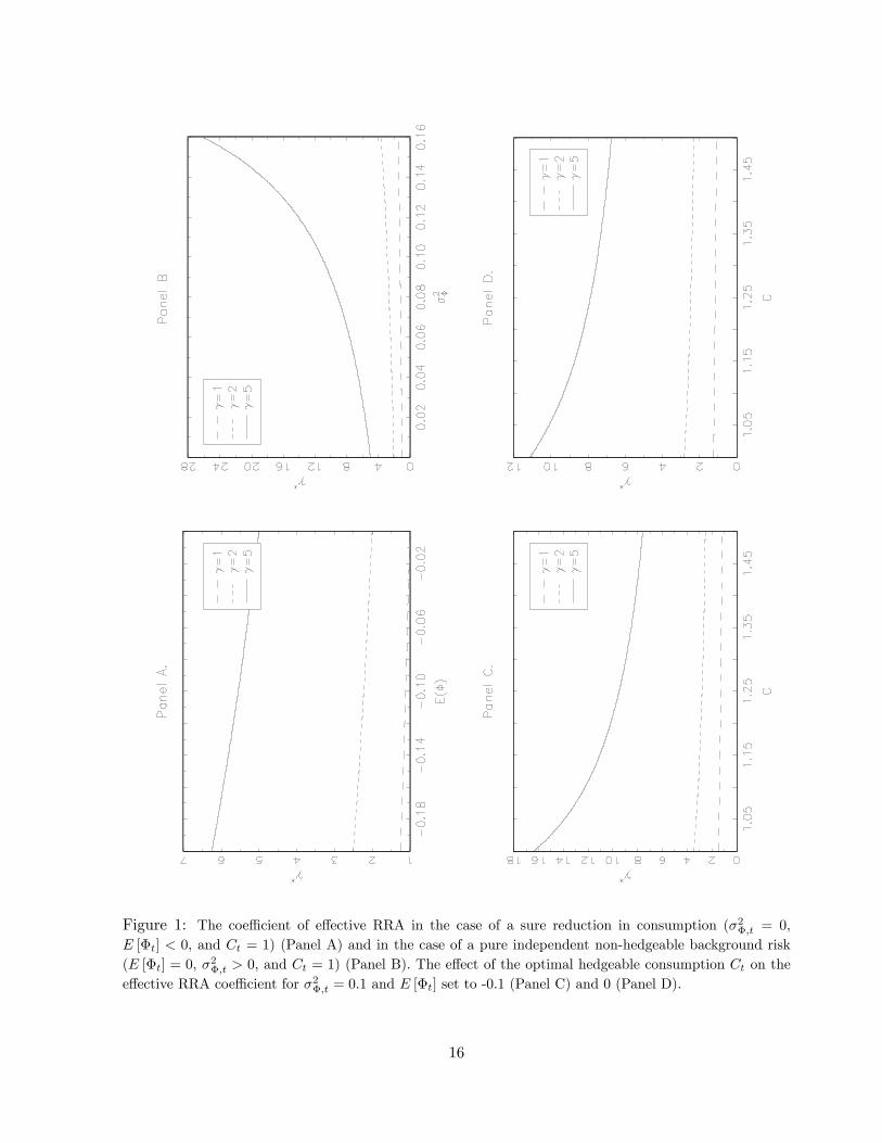
Figure 1: The coe¢ cient of e¤ective RRA in the case of a sure reduction in consumption (�2�;t = 0,E [�t] < 0, and Ct = 1) (Panel A) and in the case of a pure independent non-hedgeable background risk(E [�t] = 0, �2�;t > 0, and Ct = 1) (Panel B). The e¤ect of the optimal hedgeable consumption Ct on thee¤ective RRA coe¢ cient for �2�;t = 0:1 and E [�t] set to -0.1 (Panel C) and 0 (Panel D).

16

with background risk the marginal utility of consumption is always well-de�ned at economically

plausible (less than 10) values of the original utility curvature parameter . As to the volatility of

the estimate of the e¤ective RRA coe¢ cient, the results presented in Figure 1 suggest that the es-

timate of e¤ective RRA in the model with background risk is unlike to by highly volatile over time

unless the utility curvature parameter is quite high (say, greater than �ve). Although the Camp-

bell and Cochrane (1999) habit formation model and the consumption CAPM with background

risk are based on very di¤erent assumptions, in the both models the agent�s attitudes towards

�nancial risk are time varying, whereas RRA is constant over time in the standard consumption

CAPM.

An important determinant of the investor�s consumption and savings decisions is the EIS in

consumption, which measures the sensitivity of changes in the investor�s expected consumption

growth rate between two periods to changes in interest rates. The EIS can be computed as the

derivative of planned log consumption growth with respect to the log return on the risk-free asset.

As argued above, the representative agent with utility u (�) facing background risk has the sameoptimal hedgeable consumption plan as the representative agent with utility g (�) in the no back-ground risk environment. This suggests that the willingness of the investor with utility u (�) tomove consumption between time periods in response to changes in the interest rate under back-

ground risk will be identical to that of the investor with utility g (�) in the absence of backgroundrisk, implying that the EIS in the model with an independent non-hedgeable background risk and

utility u (�), which we write as �u;t+1, is the same as in the case when there is no background riskand utility is g (�), i.e.,

�u;t+1 =@Et [�ct+1]

@rf;t+1= �g;t+1 =

1

�t+16 1

t+1; (53)

where �ct+1 = ln (Ct+1=Ct) and rf;t+1 = ln (Rf;t+1). The inequality is strict in the presence of

background risk.

The above result implies that the model with background risk enables us to disentangle the

coe¢ cient of pure RRA and the EIS in the expected utility framework. Another implication is

that, when the agent�s preferences exhibit risk vulnerability, we can get a low value of the EIS

even if the original utility function is not very concave, while in the standard consumption CAPM

we need a large value of the utility curvature parameter to get a low value of elasticity. Since, as

we showed above, the e¤ective RRA coe¢ cient may change over time depending on the �rst two

unconditional moments of the non-hedgeable consumption distribution, so does the EIS.

17

3 Empirical investigation

3.1 The data

3.1.1 The consumption data

We use quarterly consumption data from the CEX, produced by the US Bureau of Labor Statistics

(BLS). The CEX data available cover the period from 1980:Q1 to 2003:Q4. It is a collection of

data on approximately 5000 households per quarter in the US. Each household in the sample

is interviewed every three months over �ve consecutive quarters (the �rst interview is practice

and is not included in the published data set). As households complete their participation, they

are dropped and new households move into the sample. Thus, each quarter about 20% of the

consumer units are new. The second through �fth interviews use uniform questionnaires to collect

demographic and family characteristics as well as data on quarterly consumption expenditures for

the previous three months made by households in the survey (demographic variables are based

upon heads of households). Various income information and information on the employment

of each household member is collected in the second and �fth interviews. As opposed to the

Panel Study of Income Dynamics (PSID), which o¤ers only food consumption data on an annual

basis, the CEX contains highly detailed data on quarterly consumption expenditures.14 The

CEX attempts to account for an estimated 70% of total household consumption expenditures.

Since the CEX is designed with the purpose of collecting consumption data, measurement error

in consumption is likely to be smaller for the CEX consumption data compared with the PSID

consumption data.

As suggested by Attanasio and Weber (1995), Brav et al. (2002), and Vissing-Jorgensen

(2002), we drop all consumption observations for the years 1980 and 1981 because the quality of

the CEX consumption data is questionable for this period. Thus, our sample covers the period

from 1982:Q1 to 2003:Q4. Following Brav et al. (2002), in each quarter we drop households that

do not report or report a zero value of consumption of food, consumption of nondurables and

services, or total consumption. We also delete from the sample nonurban households, households

residing in student housing, households with incomplete income responses, households that do not

have a �fth interview, and households whose head is under 19 or over 75 years of age.

In the �fth (�nal) interview, the household is asked to report the end-of-period estimated

market value of all stocks, bonds, mutual funds, and other such securities held by the consumer

unit on the last day of the previous month as well as the di¤erence in this estimated market value

compared with the value of all securities held a year ago last month. Using these two values,

we calculate each consumer unit�s asset holdings at the beginning of a 12-month recall period in

14Food consumption is likely to be one of the most stable consumption components. Furthermore, as is pointedout by Carroll (1994), 95% of the measured food consumption in the PSID is noise due to the absence of interviewtraining.

18

constant 2005 dollars. We consider four sets of households based on the reported amount of asset

holdings at the beginning of a 12-month recall period. The �rst set consists of all households

regardless of the reported amount of asset holdings. To take into account the limited participation

of households in the capital market, we also consider households that report a positive amount

of total asset holdings (the second set), households that report total assets equal to or exceeding

$1000 (the third set), and, �nally, households that report total assets equal to or exceeding $5000

(the fourth set).

As is conventional in the literature, the consumption measure used in this paper is consumption

of nondurables and services. For each household, we calculate quarterly consumption expenditures

for all the disaggregate consumption categories o¤ered by the CEX. Then, we de�ate obtained

values in 2005 dollars with the CPI�s (not seasonally adjusted, urban consumers) for appropri-

ate consumption categories.15 Aggregating the household�s quarterly consumption across these

categories is made according to the National Income and Product Account (NIPA) de�nition of

consumption of nondurables and services. The household�s per capita consumption growth be-

tween two quarters t and t + 1 is de�ned as the ratio of the household�s per capita consumption

in quarters t + 1 and t.16 To mitigate observation error in individual consumption, we subject

the households to a consumption growth �lter and use the conventional z-score method to de-

tect outliers. Following common practice for highly skewed data sets, in each time period we

consider the consumption growth rates with z-scores greater than two in absolute value to be

due to reporting or coding errors and remove them from the sample. The household�s per capita

consumption growth is deseasonalized using the multiplicative adjustments obtained from the per

capita consumption growth rate, as explained below.

The consumption of the representative agent within each set of households is calculated as

the average per capita consumption expenditures of the households in the set. For each set of

households, the per capita consumption growth is seasonally adjusted by using multiplicative

adjustments obtained from the X-12 procedure.

3.1.2 The returns data

The nominal quarterly value-weighted market capitalization-based decile index returns (capital

gain plus all dividends) on all stocks listed on the NYSE, AMEX, and Nasdaq are from the

Center for Research in Security Prices (CRSP) of the University of Chicago. Smallest stocks are

placed in portfolio 1 and the largest in portfolio 10. The nominal quarterly value-weighted returns

on the �ve NYSE, AMEX, and Nasdaq industry portfolios ((i) consumer durables, nondurables,

wholesale, retail, and some services (laundries, repair shops), (ii) manufacturing, energy, and

15The CPI series are obtained from the BLS through CITIBASE.16The quarterly consumption growth between dates t and t+ 1 is calculated if consumption is not equal to zero

for both of the quarters (missing information is counted as zero consumption).

19

utilities, (iii) business equipment, telephone and television transmission, (iv) healthcare, medical

equipment, and drugs, and (v) other) and the ten NYSE, AMEX, and Nasdaq industry portfolios

((i) consumer nondurables, (ii) consumer durables, (iii) manufacturing, (iv) oil, gas, and coal

extraction and products, (v) business equipment, (vi) telephone and television transmission, (vii)

wholesale, retail, and some services (laundries, repair shops), (viii) healthcare, medical equipment,

and drugs, (ix) utilities, and (x) other) are from Kenneth R. French�s web page.

The nominal quarterly risk-free rate is the 3-month US Treasury Bill secondary market rate

on a per annum basis obtained from the Federal Reserve Bank of St. Louis. In order to convert

from the annual rate to the quarterly rate, we raise the 3-month Treasury Bill return on a per

annum basis to the power of 1/4.

The real quarterly returns are calculated as the quarterly nominal returns divided by the 3-

month in�ation rate based on the de�ator de�ned for consumption of nondurables and services.

We calculate the equity premium as the di¤erence between the real equity return and the real

risk-free rate.

Table I reports the descriptive statistics for the data set used in estimation.

3.2 The estimation procedure

We use Hansen and Jagannathan�s (HJ, hereafter) (1991) volatility bounds to assess the empir-

ical performance of the model with background risk. Our benchmark models are the standard

representative-agent consumption CAPM and the consumption CAPM in which the SDF is the

Taylor expansion of the equally weighted sum of the households�marginal rates of substitution up

to cubic terms as proposed in Brav et al. (2002).

In the standard consumption CAPM, the SDF is

Mt+1 = �

�Ct+1Ct

���: (54)

The pricing kernel in Brav et al. (2002) is

Mt+1 = �q��t+1

"1 +

� (�+ 1)

2N

NXi=1

�qi;t+1qt+1

� 1�2� � (�+ 1) (�+ 2)

6N

NXi=1

�qi;t+1qt+1

� 1�3#

; (55)

where qi;t+1 is the household i�s consumption growth rate between quarters t and t + 1, qt+1is the cross-sectional mean of the consumption growth rate, qt+1 = N�1PN

i=1 qi;t+1, and � is

the utility curvature parameter. Since Brav et al. (2002) estimate the agent�s RRA coe¢ cient

� under the assumption of background risk (which is, in contrast to our approach, is taken into

account by considering the �rst three cross-sectional moments of the distribution of the household�s

consumption growth rate, while we consider a single representative agent facing an independent

non-hedgeable adverse background risk), the parameter � in their framework is somewhat similar

to the pure RRA coe¢ cient.

20

As we showed in Section 2.2, the SDF in the consumption CAPM with background risk is

Mt+1 = �

�E� [Ct+1]

E� [Ct]

�� 1� +12 &

2�;t+1

1� +12 &

2�;t

!� : (56)

The parameters of this pricing kernel cannot be estimated without knowledge of the �rst two

unconditional moments of the hypothetical distribution of the representative agent�s consumption,

which are unobservable. We overcome this problem by using the estimated values of these variables

instead of the true values. To estimate E� [Ct] and &2�;t for all t, we adopt the following approach.

As we mentioned in Section 2.1, the consumption CAPM with background risk described in this

paper is based on the assumption of market completeness for uncertainty about the return on

the risky asset and market incompleteness for the independent background risk. Hence, we may

assume that in the absence of the independent non-hedgeable background risk the agents are able

to equalize, state by state, their intertemporal marginal rates of substitution in consumption.

This implies that CRRA utility maximizing investors are able to equalize, state by state, their

hedgeable consumption growth rates and therefore variations in the observed consumption growth

rate for individual investors may be attributed to di¤erent non-hedgeable background risks the

agents faced in the time period under consideration.

We assume that the representative agent may be subject to the same independent non-

hedgeable background risks as individual investors and hence the hypothetical distribution of the

consumption growth rate for the representative agent may be well approximated by the observed

distribution of the individual consumption growth rate. Under this assumption, we calculate Ct;�,

� = 1; :::; N , as

Ct;� = Ct�1qi;t; � = i = 1; :::; N; (57)

where qi;t is the observed real consumption growth rate for household i between quarters t�1 andt.

We then estimate E� [Ct] and &2�;t for all t as, respectively, the mean and the normalized

variance of the generated in this manner hypothetical distribution of the representative agent�s

consumption:

\E� [Ct] = N�1NX�=1

Ct;�; (58)

b&2�;t = N�1NX�=1

Ct;� � \E� [Ct]

\E� [Ct]

!2: (59)

Substituting the \E� [Ct] and the b&2�;t for the E� [Ct] and the &2�;t in (56) yields the SDFMt+1 = �

\E� [Ct+1]\E� [Ct]

!� 1� +1

2 b&2�;t+11� +1

2 b&2�;t!�

: (60)

21

Then, the SDF in the model with background risk becomes testable.

For each of the above SDFs ((54), (55), and (60)), we test the conditional Euler equations for

the excess returns on risky assets

Et [Zt+1Mt+1] = 0 (61)

and the risk-free rate

Et [Rf;t+1Mt+1] = 1; (62)

where Zt+1 is the K-vector of time t + 1 excess returns with elements Zi;t+1 = Ri;t+1 � Rf;t+1,i = 1; :::;K, and 0 is the K-vector of zeroes.

Denote the vector of error terms in the Euler equation for the excess returns as �t+1, �t+1 =

Zt+1Mt+1, and the error term in the Euler equation for the risk-free rate as "f;t+1, "f;t+1 =

Rf;t+1Mt+1 � 1. Equations (61) and (62) imply that the error terms in the Euler equations areorthogonal to any variable xt in the agent�s time t information set and hence, at the true parameter

vector,

E [�t+1xt] = 0; (63)

E ["f;t+1xt] = 0: (64)

Since the true Euler equation error is contemporaneously uncorrelated with any lagged variable,

we take as instruments xt a constant, the aggregate per capita consumption growth rate, the

returns on the CRSP equally and value-weighted indices, and the risk-free rate of return. All the

variables are lagged one and two periods.17

A lower volatility bound for admissible SDFs Mat+1 (m), which have unconditional mean m

and satisfy the orthogonality condition (63), can then be calculated as

��Mat+1 (m)

�=�m2E [Zt+1xt]

0��1E [Zt+1xt]�1=2

; (65)

where � is the unconditional variance-covariance matrix of Zi;t+1xt.

Following HJ (1991), we �rst treat m as an unknown parameter and look for the values of the

SDF parameters, at which a considered SDF Mt+1 (m) satis�es the volatility bound (65), i.e.,

� (Mt+1 (m))

��Mat+1 (m)

� > 1 (66)

or, equivalently,

� (Mt+1 (m))

��Mat+1 (m)

� = ��fMt+1 (em)��em2E [Zt+1xt]

0��1E [Zt+1xt]�1=2 > 1; (67)

17As emphasized by Hansen and Singleton (1982), time aggregation can make instruments correlated with theerror term in the Euler equation. Hall (1988) argues that the use of variables lagged two periods helps to reduce thiscorrelation as well as the e¤ect of the mismatching of measurement time periods with planning time periods. Asargued by Epstein and Zin (1991), the use as instruments variables lagged two periods require weaker assumptionson the information structure of the problem compared with the case of variables lagged one period. Ogaki (1988)demonstrates that the use of the second lag is consistent with the information structure of a monetary economywith cash-in-advance constraints.

22

where fMt+1 =Mt+1

�(68)

and em = T�1PT�1t=0

fMt+1.

Denote as � the utility curvature parameter in the SDF fMt+1.18 For each instrument xt, we

look for the smallest value of the utility curvature parameter �, say b� (xt), at which inequality (67)holds.

Then, we �nd the optimal value of the estimate of the curvature parameter as the largest such

value of b� (xt):19 b�opt = maxfxtg

b� (xt) : (69)

This value of b� (xt) is optimal in the sense that at � = b�opt the conditional Euler equation (61)for the given set of risky assets holds for any instrument in the chosen instrument set.20 Because

� = � in SDF (54), � = � in SDF (55), and � = in SDF (60), b�opt is the estimate of the pureRRA coe¢ cient in the corresponding model. In the standard consumption CAPM, the e¤ective

RRA coe¢ cient coincides with the coe¢ cient of pure RRA and hence b�opt is also the estimate ofthe e¤ective RRA coe¢ cient.

Denote as xoptt the instrument xt, for which b� (xt) = b�opt. Since at the true parameter vector theorthogonality condition (64) holds for any xt, it also holds for x

optt and therefore this orthogonality

condition can be written as

E[(Rf;t+1Mt+1 � 1)xoptt ] = 0 (70)

or, equivalently,

�E[Rf;t+1fMt+1xoptt ] = E[xoptt ]: (71)

Because we use a time series of the return on the risk-free asset, we estimate the subjective

time discount factor � as b� = PT�1t=0 x

opttPT�1

t=0 Rf;t+1fMt+1(b�opt)xoptt ; (72)

where fMt+1(b�opt) is the value of fMt+1 calculated at � = b�opt.As a result, we obtain the estimates of the pricing kernel parameters (b�opt and b�), at which

the conditional Euler equations (61) and (62) hold for the given set of instrumental variables and

therefore the SDF is consistent with a given set of the excess returns on risky assets and the

risk-free rate of return.18� = � in (54), � = � in (55), and � = in SDF (60).19This approach is somewhat similar to that in Bekaert and Liu (2004).20Because b� (xt) 6 b�opt for any instrument xt and for any instrument the value of b� (xt) is such that the pricing

kernel satis�es the lower volatility bound at any � > b� (xt), it also satis�es the lower volatility bound at � = b�opt forany variable in the set of instruments.

23

As argued in Section 2.4, in the model with background risk the e¤ective RRA coe¢ cient

di¤ers from the utility curvature parameter (the coe¢ cient of pure RRA) and is

�t = Ct

E� [Ct]

�1� + 2

2&2�;t

�� �1�1� + 1

2&2�;t

� : (73)

When estimating the coe¢ cient of e¤ective RRA in the consumption CAPM with background

risk, we follow Kimball (1993) and Franke et al. (1998) and assume that the background risk is

actuarially neutral, i.e., E [�t] = 0. Under this assumption, an estimator of the e¤ective RRA

coe¢ cient is

b �t = b opt�1� b opt + 22b&2�;t��b opt�1�1� b opt + 12

b&2�;t�b opt ; (74)

where b&2�;t is from (59) and b opt is b�opt obtained for the pricing kernel (60) as explained above.3.3 The results

We test the candidate SDFs using three di¤erent sets of risky assets: (i) the CRSP market

capitalization-based decile portfolios (we also consider two subsets of this set of risky assets,

namely the small stock portfolios (deciles 1-5) and the large stock portfolios (deciles 6-10)), (ii)

the �ve NYSE, AMEX, and Nasdaq industry portfolios, and (iii) the ten NYSE, AMEX, and

Nasdaq industry portfolios. For each set of risky assets, the estimation results are reported for

the four sets of households de�ned in Section 3.1.1.

The estimation results for the unconditional and conditional versions of each model are quite

similar with slightly higher point estimates of the pure RRA coe¢ cient for the conditional version.

This result is robust to the set of risky assets and the household layer. Since the conditional

approach provides a more restrictive test of the model performance, in the following we focus on

the results obtained for the conditional Euler equations. The results for the conditional versions

of the standard model, the model with the SDF proposed in Brav et al. (2002), and the model

with background risk are reported in Table II. The column labeled "SM" in this table shows the

results for the standard model, the column labeled "BCG" presents the estimation results for the

model with the pricing kernel proposed in Brav et al. (2002), and the column labeled "MBR"

shows the estimates of the parameters for the model with background risk.

The results for the conditional standard consumption CAPM can be summarized as follows.

When all households regardless of the reported amount of asset holdings are considered, the

estimate of pure RRA is unrealistically high (from 16.6 to 26.0),21 while the estimate of the

subjective time discount factor is implausibly low (from 0.81 to 0.90).22 When limited asset

21For this model, the e¤ective and pure RRA coe¢ cients coincide and hence the estimate of � in the standardmodel is the estimate of the both coe¢ cients.22Brav et al. (2002) also obtain low estimates of the subjective time discount factor in the standard consumption

CAPM and argue that this result is due to error in the observed per capita consumption, which severely biasesdownward the estimated subjective time discount factor in the standard consumption CAPM.

24

market participation is taken into account, as expected, we obtain the estimates of pure RRA

aversion that are quite lower than the estimates obtained for all households. These estimates

range from 7.4 to 14.0 and hence are still too high to be recognized as economically realistic. The

obtained estimates of the subjective time discount factor are greater and more realistic (they range

from 0.90 to 0.99) compared with the estimates obtained for the whole set of households.

The model with the SDF expressed in terms of the cross-sectional mean, variance, and skewness

of the household consumption growth rate, as proposed in Brav et al. (2002), explains the cross-

sectional equity premium with the value of pure RRA that ranges from 5.6 to 8.9. These estimates

are lower than the values of the pure RRA coe¢ cient implied by the standard consumption CAPM,

but are still unrealistically high. Another drawback of this pricing kernel is that it yields an

estimate of the subjective time discount factor, which is implausibly low. This estimate is in the

range from 0.55 to 0.68.23

In contrast to the standard model and the model proposed in Brav et al. (2002), the consump-

tion CAPM with background risk explains the cross-section of asset returns and the risk-free rate

at much lower values of the pure RRA coe¢ cient and more realistic values of the subjective time

discount factor. Under the assumption that the conditional Euler equations hold for all agents

regardless of the reported amount of asset holdings, the estimate of the coe¢ cient of pure RRA

ranges from 4.8 to 5.7 and the estimate of the subjective time discount factor ranges from 0.92 to

0.96. Under limited asset market participation, the estimates of pure RRA are between 3.7 and

5.2 and the estimates of the subjective time discount factor are in the range from 0.89 to 0.96.

The estimate of the pure RRA coe¢ cient decreases as the threshold value in the de�nition of asset

holders is raised.

To investigate whether the estimation results are sensitive to the size of stocks under consider-

ation, we test the three models separately for the decile 1-5 and decile 6-10 portfolios. Our result

is that the stock size does not a¤ect signi�cantly the performance of the models. As for the whole

set of the market capitalization-based decile portfolios, for any subset of this set of risky assets

both the standard model and the model proposed by Brav et al. (2002) yield too high estimates

of pure RRA and too low estimates of the subjective discount factor, while for the model with

background risk the estimates of the both parameters are within the acceptable range of values.

In the consumption CAPM with background risk, the estimate of the e¤ective RRA di¤ers

from the estimate of the coe¢ cient of pure RRA (the utility curvature parameter ) and may

change over time. We calculate the coe¢ cient of e¤ective RRA in the model with background risk

for each quarter over the period from 1982:Q3 to 2003:Q4. As expected, the estimates of e¤ective

23 In Brav et al. (2002), the estimated subjective time discount factor in the pricing kernel that captures the mean,variance, and skewness of the cross-sectional distribution of the household consumption growth is also very low andbelow the estimate of the subjective time discount factor obtained for the standard model. The authors explain thisby the fact that the observation error in household consumption is substantially higher than the observation errorin per capita consumption.

25

RRA are greater than the estimates of the pure RRA coe¢ cient and are not highly volatile.

When estimating the proportion of the risk premium due to the background risk, we use the

time average estimate of the e¤ective RRA coe¢ cient under background risk as the value of �tin (44). The result is that for di¤erent sets of risky assets and sets of households the background

risk accounts for from 34 to 44 percent of the risk premium.

Table II reports the estimates of the correlation between the e¤ective RRA coe¢ cient and the

market premium, which is proxied by the real excess return on the value-weighted CRSP market

portfolio over the risk-free rate, as well as the estimates of the correlation between the coe¢ cient

of e¤ective RRA and the normalized variance of the non-hedgeable consumption, &2�;t. Because

the sampling distribution of Pearson�s correlation coe¢ cient r might be asymmetric, we use the

Fisher transformation when testing the null hypothesis that the population correlation coe¢ cient

� = 0.24 This transformation is applied to the sample correlation r and is de�ned by

z = 0:5 ln

�1 + r

1� r

�: (75)

The random variable z in (75) is normally distributed with standard deviation 1=pT � 3, where

T is the sample size.

We �nd that in the model with background risk the correlation of the e¤ective RRA coe¢ cient

with the market premium is very low and not statistically di¤erent from zero at any conventional

level of signi�cance. This result is not surprising because, as follows from equation (74), the agent�s

e¤ective RRA is only a function of the utility curvature parameter (which is constant over time)

and the normalized variance of the non-hedgeable consumption, &2�;t (which is assumed to be

uncorrelated with the market premium). The correlation of the e¤ective RRA coe¢ cient with

the normalized variance of the non-hedgeable consumption, &2�;t, is close to one and signi�cantly

di¤erent from zero at the 5% level of signi�cance.

The null hypothesis of serial correlation of the e¤ective RRA coe¢ cient is rejected statisti-

cally at any conventional level of signi�cance for the entire set of households regardless of the

reported amount of asset holdings. Under limited asset market participation, in most cases the

�rst-order autocorrelation coe¢ cient is positive and signi�cantly di¤erent from zero at the 10%

level (what might be due to serial correlation in the normalized variance of the non-hedgeable

consumption), while the second-order autocorrelation coe¢ cient is always low in absolute value

and not signi�cantly di¤erent from zero at any conventional signi�cance level.25

Using the property that the EIS is equal to the reciprocal of the e¤ective RRA coe¢ cient, we

calculate for each quarter the EIS in the consumption CAPM with background risk as the inverse

24See Fisher (1915, 1921).25Fuller (1976) shows that under the IID null hypothesis the sample autocorrelation coe¢ cients are asymptotically

independent and normal with mean zero and standard deviation 1=pT , i.e., b�k a� N (0; 1=T ), where �k is the kth-

order autocorrelation coe¢ cient.

26

of the coe¢ cient of e¤ective RRA obtained for this quarter under the assumption of background

risk. The result is that the estimates of the EIS are only slightly volatile over time with the average

value in the range from 0.10 to 0.19.

4 Concluding Remarks

In this paper, we assumed an economy in which a single representative investor faces, in addition to

the insurable �nancial risk, an independent non-hedgeable adverse background risk. We presented

empirical evidence that, in contrast to the previously proposed incomplete consumption insurance

models, the asset-pricing model with the SDF calculated as the discounted ratio of expectations

of marginal utilities over the non-hedgeable consumption states at two consecutive dates jointly

explains the cross-section of risky asset excess returns and the risk-free rate with economically

plausible values of the pure RRA coe¢ cient and the subjective time discount factor. Consistently

with earlier results, we reject empirically the model based on the assumption of no background

risk (the standard consumption CAPM). The results are robust across di¤erent sets of stock-

returns and threshold values in the de�nition of asset holders. Since the important components

of the pricing kernel are the �rst two unconditional moments of the distribution of the non-

hedgeable consumption, this supports the hypothesis that the independent non-hedgeable adverse

background risk can account for the market premium and the return on the risk-free asset.

References

[1] Aiyagari, S. Rao, and Mark Gertler, 1991, Asset returns with transactions costs and uninsured

individual risk, Journal of Monetary Economics 27, 311-331.

[2] Attanasio, Orazio P., and Guglielmo Weber, 1995, Is consumption growth consistent with

intertemporal optimization? Evidence from the Consumer Expenditure Survey, Journal of

Political Economy 103, 1121-1157.

[3] Bakshi, Gurdip S., and Zhiwu Chen, 1996, The spirit of capitalism and stock-market prices,

American Economic Review 86, 133-157.

[4] Balduzzi, Pierluigi, and Tong Yao, 2007, Testing heterogeneous-agent models: An alternative

aggregation approach, Journal of Monetary Economics 54, 369-412.

[5] Bekaert, Geert, and Jun Liu, 2004, Conditioning information and variance bounds on pricing

kernels, Review of Financial Studies 17, 339-378.

[6] Bewley, Truman F., 1982, Thoughts on tests of the intertemporal asset pricing model, working

paper, Evanston, Ill.: Northwestern University.

27

[7] Brav, Alon, George M. Constantinides, and Christopher C. Géczy, 2002, Asset pricing with

heterogeneous consumers and limited participation: Empirical evidence, Journal of Political

Economy 110, 793-824.

[8] Breeden, Douglas T., 1979, An intertemporal asset pricing model with stochastic consumption

and investment opportunities, Journal of Financial Economics 7, 265�296.

[9] Campbell, John Y., and John Cochrane, 1999, By force of habit: a consumption-based ex-

planation of aggregate stock market behavior, Journal of Political Economy 107, 205-251.

[10] Campbell, John Y., Andrew W. Lo, and A. Craig MacKinlay, 1997, The Econometrics of

Financial Markets (Princeton University Press, Princeton).

[11] Carroll, Christopher D., 1994, How does future income a¤ect current consumption, Quarterly

Journal of Economics 109, 111-147.

[12] Cogley, Timothy, 2002, Idiosyncratic risk and the equity premium: Evidence from the Con-

sumer Expenditure Survey, Journal of Monetary Economics 49, 309-334.

[13] Courbage, Christophe, and Béatrice Rey, 2007, Precautionary saving in the presence of other

risks, Economic Theory 32, 417-424.

[14] Drèze, Jacques H., and Franco Modigliani, 1972, Consumption decision under uncertainty,

Journal of Economic Theory 5, 308-335.

[15] Epstein, Larry G., and Stanley E. Zin, 1991, Substitution, risk aversion and the temporal be-

havior of consumption and asset returns: An Empirical analysis, Journal of Political Economy

99, 263-288.

[16] Fisher, Ronald Aylmer, 1915, Frequency distribution of the values of the correlation coe¢ cient

in samples of an inde�nitely large population, Biometrika 10, 507-521.

[17] Fisher, Ronald Aylmer, 1921, On the �probable error�of a coe¢ cient of correlation deduced

from a small sample, Metron 1, 3-32.

[18] Franke, Guenter, Richard C. Stapleton, and Marti G. Subrahmanyam, 1998, Who buys and

who sells options: The role of options in an economy with background risk, Journal of Eco-

nomic Theory 82, 89-109.

[19] Fuller, Wayne A., 1976, Introduction to Statistical Time Series (New York: Wiley).

[20] Gollier, Christian, 2001, The economics of risk and time (MIT Press, Cambridge, MA).

28

[21] Gordon, Stephen, and Pascal St-Amour, 2004, Asset returns and state-dependent risk pref-

erences, Journal of Business and Economic Statistics 22, 241-252.

[22] Hall, Robert E., 1988, Intertemporal substitution in consumption, Journal of Political Econ-

omy 96, 339-357.

[23] Hansen, Lars Peter, and Ravi Jagannathan, 1991, Implications of security market data for

models of dynamic economies, Journal of Political Economy 99, 225-262.

[24] Hansen, Lars Peter, and Kenneth J. Singleton, 1982, Generalized instrumental variables es-

timation of nonlinear rational expectations models, Econometrica 50, 1269-1286.

[25] Heaton, John, and Deborah Lucas, 1996, Evaluating the e¤ects of incomplete markets on risk

sharing and asset pricing, Journal of Political Economy 104, 443-487.

[26] Heaton, John, and Deborah Lucas, 1997, Market frictions, savings behavior, and portfolio

choice, Macroeconomic Dynamics 1, 76-101.

[27] Huggett, Mark, 1993, The risk-free rate in heterogeneous-agent incomplete-insurance

economies, Journal of Economic Dynamics and Control 17, 953-969.

[28] Jacobs, Kris, 1999, Incomplete markets and security prices: Do asset-pricing puzzles result

from aggregation problems?, Journal of Finance 54, 123-163.

[29] Kihlstrom, Richard E., David Romer, and Steve Williams, 1981, Risk aversion with random

initial wealth, Econometrica 49, 911-920.

[30] Kimball, Miles S., 1993, Standard risk aversion. Econometrica 61, 589-611.

[31] Kimball, Miles S., 1992, Precautionary motives for holding assets. In: Newmann, P., Falwell,

J. (eds.) The new palgrave dictionary of money and �nance, pp. 158�161. London: MacMillan.

[32] Kimball, Miles S., 1990, Precautionary savings in the small and in the large, Econometrica

58, 53-73.

[33] Kocherlakota, Narayana R., and Luigi Pistaferri, 2008, Asset pricing implications of Pareto

optimality with private information, working paper.

[34] Leland Hayne E., 1968, Saving and uncertainty: The precautionary demand for saving, Quar-

terly Journal of Economics 82, 465-473.

[35] Lucas, Deborah, 1994, Asset pricing with undiversi�able income risk and short sales con-

straints: Deepening the equity premium puzzle, Journal of Monetary Economics 34, 325-341.

29

[36] Lucas Jr., Robert E., 1978, Asset prices in an exchange economy, Econometrica 46, 1429�1445.

[37] Mankiw, N. Gregory, 1986, The equity premium and the concentration of aggregate shocks,

Journal of Financial Economics 17, 211-219.

[38] Mehra, Rajnish, and Edward C. Prescott, 1985, The equity premium: A puzzle, Journal of

Monetary Economics 15, 145-162.

[39] Nachman, David C., 1982, Preservation of "more risk averse" under expectations, Journal of

Economic Theory 28, 361-368.

[40] Ogaki, Masao, 1988, Learning about preferences from time trends, Ph.D. Dissertation, Uni-

versity of Chicago.

[41] Poon, Ser-Huang, and Richard C. Stapleton, 2005, Asset Pricing in Discrete Time: A Com-

plete Market Approach (Oxford University Press, Oxford, New York).

[42] Sandmo, Agnar, 1970, The e¤ect of uncertainty on saving decisions, The Review of Economic

Studies 37, 353-360.

[43] Telmer, Chris, 1993, Asset-pricing puzzles and incomplete markets, Journal of Finance 48,

1803-1832.

[44] Vissing-Jorgensen, Annette, 2002, Limited asset market participation and the elasticity of

intertemporal substitution, Journal of Political Economy 110, 825-853.

[45] Weil, Philippe, 1989, The equity premium puzzle and the risk-free rate puzzle, Journal of

Monetary Economics 24, 401-421.

30

Table I. Descriptive Statistics

In this table, CGRt is the aggregate per capita consumption growth rate, &2�;t is the normalized varianceof the non-hedgeable consumption, RVW;t and REW;t are the CRSP value- and equal-weighted indices,respectively, Rf;t is the risk-free rate of return, RDi;t (i = 1; :::; 10) are the returns on the CRSP marketcapitalization-based decile portfolios, R5Ii;t (i = 1; :::; 5) and R10Ii;t (i = 1; :::; 10) are the returns on the�ve and ten industry portfolios, respectively. The sample period is 1982:Q1 to 2003:Q4.

Variable Minimum Median Maximum Mean St.Dev. Skewness

A. Consumption

A.1 All Households

CGRt 0.9039 0.9895 1.0664 0.9897 0.0339 0.0596&2�;t 0.0468 0.0721 0.1446 0.0733 0.0136 1.9611

A.2 Households with Total Assets > $0

CGRt 0.8835 1.0011 1.1348 0.9972 0.0500 0.0867&2�;t 0.0292 0.0731 0.1306 0.0732 0.0207 0.4479

A.3 Households with Total Assets > $1000

CGRt 0.8774 0.9973 1.1427 0.9965 0.0510 0.0901&2�;t 0.0292 0.0726 0.1306 0.0731 0.0200 0.3351

A.4 Households with Total Assets > $5000

CGRt 0.8776 0.9999 1.1618 0.9963 0.0552 0.2694&2�;t 0.0320 0.0765 0.1546 0.0764 0.0235 0.7064

B. Asset Returns

B.1 Market Portfolio Returns and the Risk-Free Rate

RVW;t 0.7633 1.0346 1.2059 1.0269 0.0872 -0.4703REW;t 0.7033 1.0257 1.3176 1.0321 0.1161 -0.0395Rf;t 0.9933 1.0056 1.0178 1.0053 0.0048 0.2153

B.2 Decile Portfolio Returns

RD1;t 0.7644 1.0434 1.2164 1.0363 0.0880 -0.4554RD2;t 0.7199 1.0262 1.2855 1.0302 0.1152 -0.3173RD3;t 0.7584 1.0364 1.2256 1.0297 0.0883 -0.5788RD4;t 0.7658 1.0242 1.2436 1.0236 0.0780 -0.6265RD5;t 0.6518 1.0381 1.3968 1.0303 0.1436 -0.1897RD6;t 0.7652 1.0398 1.2570 1.0266 0.1031 -0.2717RD7;t 0.7027 1.0321 1.3129 1.0338 0.1065 -0.1787RD8;t 0.7544 1.0320 1.2409 1.0341 0.0983 -0.2926RD9;t 0.8023 1.0352 1.2684 1.0243 0.0742 0.0048RD10;t 0.7606 1.0354 1.2076 1.0309 0.0958 -0.6319

31

Table I (continued)

Variable Minimum Median Maximum Mean St.Dev. Skewness

B.3 5 Industry Portfolio Returns

R5I1;t 0.7319 1.0410 1.2417 1.0334 0.0917 -0.3746R5I2;t 0.7917 1.0337 1.1797 1.0259 0.0702 -0.8788R5I3;t 0.6793 1.0345 1.3409 1.0287 0.1228 -0.3808R5I4;t 0.7544 1.0320 1.2409 1.0341 0.0983 -0.2926R5I5;t 0.7606 1.0354 1.2076 1.0309 0.0958 -0.6319

B.4 10 Industry Portfolio Returns

R10I1;t 0.7644 1.0434 1.2164 1.0363 0.0880 -0.4554R10I2;t 0.7199 1.0262 1.2855 1.0302 0.1152 -0.3173R10I3;t 0.7584 1.0364 1.2256 1.0297 0.0883 -0.5788R10I4;t 0.7658 1.0242 1.2436 1.0236 0.0780 -0.6265R10I5;t 0.6518 1.0381 1.3968 1.0303 0.1436 -0.1897R10I6;t 0.7652 1.0398 1.2570 1.0266 0.1031 -0.2717R10I7;t 0.7027 1.0321 1.3129 1.0338 0.1065 -0.1787R10I8;t 0.7544 1.0320 1.2409 1.0341 0.0983 -0.2926R10I9;t 0.8023 1.0352 1.2684 1.0243 0.0742 0.0048R10I10;t 0.7606 1.0354 1.2076 1.0309 0.0958 -0.6319

32

Table II

The Conditional Volatility Bounds Results

In this table, the column labeled "SM" shows the results for the standard consumption CAPM, the column labeled "BCG" presents the estimation resultsfor the model with the pricing kernel proposed in Brav et al. (2002), and the column labeled "MBR" reports the estimates of the parameters for themodel with background risk. Pure RRA is the pure RRA coefficient, δ is the subjective time discount factor, γ∗t and σ2γ∗t are respectively the sample

mean and variance of the effective RRA coefficient γ∗t , μ is the proportion of the risk premium due to the background risk, φt and σ2φt are respectivelythe sample mean and variance of the EIS. zi = 0.5ln ((1 + ri) / (1− ri)), i = 1, 2, is the Fisher z-statistic with r1 and r2 being Pearson’s coefficients ofcorrelation between γ∗t and the real excess return on the value-weighted CRSP market portfolio, RVW,t −Rf,t, and between γ∗t and ς2Φ,t, respectively. ρkis the kth-order autocorrelation coefficient of γ∗t . Asymptotic standard errors are in parentheses.

Parameter All Assets > $0 Assets > $1000 Assets > $5000SM BCG MBR SM BCG MBR SM BCG MBR SM BCG MBR

A. CRSP Market Capitalization-Based Decile Portfolios 1-10:

Pure RRA 25.9816 8.213 5.6255 13.9201 8.468 5.1311 13.9919 8.807 5.1849 12.2080 7.879 4.9121δ 0.8104 0.5549 0.9242 0.9382 0.5920 0.8890 0.9061 0.5551 0.8879 0.9033 0.5844 0.8867

γ∗t 10.1240 8.9163 8.9950 8.6133σ2γ∗t 3.8016 4.2795 3.8890 5.4466

μ 0.4443 0.4245 0.4236 0.4297

z1 -0.0955 0.0336 -0.0190 0.0592(0.1098) (0.1098) (0.1098) (0.1098)

z2 1.6398 2.0262 2.0662 1.8556(0.1098) (0.1098) (0.1098) (0.1098)

ρ1 0.1009 0.1781 0.1236 0.1884(0.1091) (0.1091) (0.1091) (0.1091)

ρ2 -0.0397 -0.0809 0.0348 0.0595(0.1091) (0.1091) (0.1091) (0.1091)

φt 0.1008 0.1169 0.1154 0.1220σ2φt 0.0001 0.0005 0.0004 0.0006

33

Table II (continued)

Parameter All Assets > $0 Assets > $1000 Assets > $5000SM BCG MBR SM BCG MBR SM BCG MBR SM BCG MBR

B. CRSP Market Capitalization-Based Decile Portfolios 1-5:

Pure RRA 19.2395 6.756 5.0651 9.8380 6.754 4.3420 9.8170 7.023 4.3524 8.6606 6.259 4.0568δ 0.8759 0.6037 0.9518 0.9817 0.6436 0.9403 0.9592 0.6109 0.9398 0.9550 0.6453 0.9397

γ∗t 8.5592 6.8930 6.8772 6.4060σ2γ∗t 1.7776 1.5752 1.3826 1.6558

μ 0.4082 0.3701 0.3671 0.3667

z1 -0.1005 0.0282 -0.0220 0.0482(0.1098) (0.1098) (0.1098) (0.1098)

z2 1.7892 2.2392 2.2880 2.0956(0.1098) (0.1098) (0.1098) (0.1098)

ρ1 0.1171 0.1835 0.1395 0.2032(0.1091) (0.1091) (0.1091) (0.1091)

ρ2 -0.0356 -0.0765 0.0424 0.0613(0.1091) (0.1091) (0.1091) (0.1091)

φt 0.1186 0.1490 0.1490 0.1609σ2φt 0.0002 0.0005 0.0005 0.0006

34

Table II (continued)

Parameter All Assets > $0 Assets > $1000 Assets > $5000SM BCG MBR SM BCG MBR SM BCG MBR SM BCG MBR

C. CRSP Market Capitalization-Based Decile Portfolios 6-10:

Pure RRA 16.5340 6.155 4.7779 8.3359 6.020 3.9608 8.2885 6.246 3.9547 7.3468 5.567 3.6550δ 0.8992 0.6302 0.9619 0.9925 0.6746 0.9568 0.9736 0.6446 0.9560 0.9695 0.6794 0.9558

γ∗t 7.8283 6.0364 5.9934 5.5163σ2γ∗t 1.2048 0.9509 0.8225 0.9249

μ 0.3897 0.3438 0.3402 0.3374

z1 -0.1028 0.0261 -0.0232 0.0436(0.1098) (0.1098) (0.1098) (0.1098)

z2 1.8684 2.3468 2.3992 2.2147(0.1098) (0.1098) (0.1098) (0.1098)

ρ1 0.1250 0.1857 0.1463 0.2087(0.1091) (0.1091) (0.1091) (0.1091)

ρ2 -0.0331 -0.0744 0.0454 0.0616(0.1091) (0.1091) (0.1091) (0.1091)

φt 0.1294 0.1693 0.1701 0.1857σ2φt 0.0002 0.0006 0.0005 0.0007

35

Table II (continued)

Parameter All Assets > $0 Assets > $1000 Assets > $5000SM BCG MBR SM BCG MBR SM BCG MBR SM BCG MBR

D. 5 Industry Portfolios:

Pure RRA 19.1530 6.737 5.0567 9.7889 6.731 4.3305 9.7670 6.999 4.3403 8.6177 6.238 4.0446δ 0.8766 0.6017 0.9541 0.9809 0.6438 0.9404 0.9586 0.6113 0.9387 0.9555 0.6458 0.9384

γ∗t 8.5372 6.8661 6.8492 6.3778σ2γ∗t 1.7575 1.5518 1.3614 1.6273

μ 0.4077 0.3693 0.3663 0.3658

z1 -0.1006 0.0282 -0.0220 0.0480(0.1098) (0.1098) (0.1098) (0.1098)

z2 1.7915 2.2424 2.2914 2.0991(0.1098) (0.1098) (0.1098) (0.1098)

ρ1 0.1174 0.1836 0.1397 0.2034(0.1091) (0.1091) (0.1091) (0.1091)

ρ2 -0.0356 -0.0764 0.0425 0.0613(0.1091) (0.1091) (0.1091) (0.1091)

φt 0.1189 0.1496 0.1496 0.1616σ2φt 0.0002 0.0005 0.0005 0.0006

36

Table II (continued)

Parameter All Assets > $0 Assets > $1000 Assets > $5000SM BCG MBR SM BCG MBR SM BCG MBR SM BCG MBR

E. 10 Industry Portfolios:

Pure RRA 20.9547 7.130 5.2252 10.8263 7.205 4.5620 10.8261 7.496 4.5832 9.5228 6.684 4.2917δ 0.8658 0.5877 0.9488 0.9726 0.6270 0.9282 0.9481 0.5927 0.9283 0.9456 0.6270 0.9274

γ∗t 8.9866 7.4208 7.4255 6.9662σ2γ∗t 2.2073 2.0919 1.8527 2.3074

μ 0.4186 0.3852 0.3828 0.3839

z1 -0.0992 0.0296 -0.0212 0.0511(0.1098) (0.1098) (0.1098) (0.1098)

z2 1.7459 2.1786 2.2253 2.0280(0.1098) (0.1098) (0.1098) (0.1098)

ρ1 0.1126 0.1821 0.1354 0.1997(0.1091) (0.1091) (0.1091) (0.1091)

ρ2 -0.0369 -0.0777 0.0404 0.0610(0.1091) (0.1091) (0.1091) (0.1091)

φt 0.1131 0.1389 0.1384 0.1487σ2φt 0.0002 0.0005 0.0005 0.0006

37