Department of Economics and Business Economics

Aarhus University

Fuglesangs Allé 4

DK-8210 Aarhus V

Denmark

Email: oekonomi@au.dk

Tel: +45 9352 1936

Asset Pricing Using Block-Cholesky GARCH and

Time-Varying Betas

Stefano Grassi and Francesco Violante

CREATES Research Paper 2021-05

Asset Pricing Using Block-Cholesky GARCH and

Time-Varying Betas

Stefano Grassi1 and Francesco Violante2

February 25, 2021

Abstract

Starting from the Cholesky-GARCH model, recently proposed by Darolles, Francq, and Lau-rent (2018), the paper introduces the Block-Cholesky GARCH (BC-GARCH). This new modeladapts in a natural way to the asset pricing framework. After deriving conditions for sta-tionarity, uniform invertibility and beta tracking, we investigate the finite sample propertiesof a variety of maximum likelihood estimators suited for the BC-GARCH by means of anextensive Monte Carlo experiment.We illustrate the usefulness of the BC-GARCH in two empirical applications. The first testsfor the presence of beta spillovers in a bivariate system in the context of the Fama and French(1993) three factor framework. The second empirical application consists of a large scaleexercise exploring the cross-sectional variation of expected returns for 40 industry portfolios.

Keywords: Cholesky decomposition, Multivariate GARCH, Asset Pricing, Time Varying Beta,

Two Pass Regression.

JEL Classification: C12, C22, C58, G12, G13

1University of Rome ’Tor Vergata’ and CREATES - Aarhus University. Phone: +390672595914 - E-mail:stefano.grassi@uniroma2.it

2CREST, GENES, ENSAE Paris, Institut Polytechnique de Paris, 5, avenue Henry Le Chatelier, TSA 96642,91764 Palaiseau cedex, France and CREATES - Aarhus University. Phone: +33 (0) 1 70 26 67 50 - E-mail:francesco.violante@ensae.fr (corresponding author)The authors would like to thank Gianluca Cubadda, Christian Francq, Edoardo Otranto, Christian Yann Robert,and Jean-Michel Zakoian for useful comments.Stefano Grassi gratefully acknowledges financial support from the University of Rome ’Tor Vergata’ under Grant“Beyond Borders” (CUP: E84I20000900005). Francesco Violante acknowledges financial support by the grant ofthe French National Research Agency (ANR), Investissements d’Avenir (LabEx Ecodec/ANR-11-LABX-0047), andof the Danish Council for Independent Research (1329-00011A). The funding organizations had no role in the studydesign, data collection and analysis, decision to publish or preparation of the manuscript.

1 Introduction

The drawbacks of testing asset pricing models with constant parameters have been long estab-

lished in the literature. Wrongly assuming parameters constancy may lead to model misspecifica-

tion, inefficiency and bias in the measurements of risk exposure and premia, potentially resulting

in the rejection of the model.

Due to its intuitive appeal and ease of implementation, the 2-Pass Cross-Sectional Regression

(2PR) approach, introduced by Fama and MacBeth (1973), has represented a standard in the

asset pricing literature to assess the cross-sectional variation of expected assets returns. Time

variation in the beta coefficients is obtained by least square estimation on a rolling sample, result-

ing in dynamic properties of the conditional betas heavily determined by the estimation window

size. Also, the rolling least square approach makes it difficult to distinguish between sampling

variability and actual time variation in the beta coefficients. Furthermore, the multi-step estima-

tion approach is subject to the well known error-in-variables problem which renders the inference

on the risk parameters challenging.

To overcome these issues Gonzalez, Nave, and Rubio (2012) propose a linear beta pricing model

with time-varying risk exposures based on a mixed frequency approach. The conditional betas

are estimated using a kernel-based weighted realized variance estimator, which exploits high-

frequency information. The model does not require specifying the dynamics of the conditional

betas, making it unsuited for forecasting and, most importantly,assuming orthogonality of the

risk factors, which is often rejected in practice.

Hansen, Lunde, and Voev (2014) construct a model based on mixed frequencies which exploit ad-

ditional information coming from non-parametric realized measures of variances and correlations.

However, because they opt for modeling correlations directly, individually, and independently

from the variances, they cannot explicitly enforce restrictions ensuring positive definiteness of

the covariance matrix of the factors-assets system beyond the bivariate dimension.

Recently Engle (2016) propose to model the dynamic conditional betas using a dynamic con-

ditional correlation GARCH (DCB-DCC). In the DCB-DCC model, the betas are recovered as

a transformation of the conditional covariance matrix of the joint factors-assets system. While

easy to implement, this indirect specification does not allow to identify the relevant drivers of

1

the betas’ evolution, and, it makes the coexistence of dynamic and constant betas challenging.

Indeed, the constancy constraint is imposed a priori rather than through parameter restrictions

on the conditional covariance dynamics.

In a recent paper, Darolles, Francq, and Laurent (2018) propose a model for time-varying betas

based on the Cholesky decomposition of the conditional covariance matrix of the factors-assets

system. This model, dubbed Cholesky-GARCH (CHAR), explicitly specifies the dynamics of the

conditional betas, and simplyfy the coexistence of constant and time-varying betas. The authors

show that the CHAR proves superior to the Engle (2016) model in terms of forecasting and beta

hedging. However, in asset pricing applications, the CHAR model shows limitations stemming

from the strictly triangular Cholesky decomposition and more so when the cross-sectional dimen-

sion of the number of assets is large.

Inspired by the CHAR model and borrowing from the decomposition used in the DCB-DCC, we

introduce a new model, the Block-Cholesky GARCH (BC-GARCH). The BC-GARCH achieves

orthogonalization between two sets of variables, namely risk factors and investment assets via a

Block-Cholesky decomposition. This provides several direct advantages over the CHAR.

First, the BC-GARCH preserves the natural hierarchy existing between risk factors and assets

without requiring any sorting within the subset of the factors and that of the assets. Conse-

quently, the conditional beta dynamics, stemming from conditioning the assets to the risk factors

and driven by the block-orthogonalized innovations, are order independent.

Second, in the asset pricing framework, the BC-GARCH allows for a coherent and parsimonious

multivariate evaluation of a multi-asset system. In the CHAR, a capital asset pricing model

(CAPM) or Fama-French linear factor model interpretation of the conditional mean equation of

the assets is straightforward when the system considered is composed by possibly multiple risk

factors but only one asset. When multiple assets are considered, the triangular structure of the

CHAR model introduces nuisance conditional betas, whose number increases quadratically with

the number of assets.1 The presence of nuisance betas inevitably rises a dimensionality problem

in large systems. Also they do not have clear interpretation as they merely account for the corre-

1For instance, in a system with k risk factors and n assets, the CHAR requires (k+n)[(k+n)−1]/2 conditionalbetas, kn of which are ”relevant” betas, i.e. measuring the exposure of assets to risk factors, while n(n− 1)/2 are”nuisance” betas linking assets to assets (as well as k(k − 1)/2 betas are nuisance conditional betas linking riskfactors to risk factors).

2

lation between assets. The BC-GARCH only requires modeling the conditional betas measuring

the exposure of assets to risk factors, whose number grows only linearly in the number of assets.

Co-movements between variables in each block are instead modeled explicitly via time-varying

covariances or correlations. Darolles, Francq, and Laurent (2018) avoid to some extent the prob-

lem by marginalizing the distribution of the multi-asset system iteratively, isolating risk factors

and a single asset at each time. Although valid, this approach limits the type of hypotheses on

the asset pricing model that can be tested, e.g. restrictions on the cross section of assets.

Third, a consequence of the triangular decomposition of the CHAR is that the magnitude of the

orthogonalized innovations tends to vanish by construction as the size of the system increases and

the higher the system’s correlation. Since these are the innovations driving the conditional betas,

they can potentially impact their dynamics in an undesirable way. The block orthogonalization

of the BC-GARCH, instead, only underlies a reduction of the magnitude of the orthogonalizad

innovations between the two blocks, while preserving it within each block independently of their

size.

Fourth, our model introduces spillovers effects in the conditional beta dynamics in an explicit,

symmetric and interpretable way. We isolate two different sources of spillovers. We define a factor

spillover a shock in a risk factor affecting the exposure of a given asset to a different risk factor.

Similarly, we define asset spillovers a shocks in one asset affecting the exposure of another asset

to a risk factors. The latter case can be implemented symmetrically across assets because the

block structure allows to model them jointly, bypassing the restriction imposed by the strictly tri-

angular structure of the CHAR and thus its inherent sequentiality. Indeed, although the CHAR

inherently allows for spillovers of shocks in the conditional betas, the Cholesky orthogonalization

makes it impossible to identify the exact source of the shock. Several suitable parametric speci-

fications for the conditional beta dynamics accounting for these features are discussed.

After deriving conditions for stationarity, uniform invertibility and beta tracking, we illustrate

the finite sample properties of a variety of maximum likelihood estimators suited for the BC-

GARCH by means of extensive Monte Carlo experiments.

In this paper we carry out two empirical applications. In the first, we test our model in the

context of the Fama and French (1993) three factor framework (3FF). The aim of this empirical

3

application is to benchmark a conditional beta specification driven only by idiosyncratic shocks

against three alternative specifications accounting for beta spillovers. We consider a bivariate

asset system composed by the Coal (C) and Petroleum-Natural Gas (P) value-weighted industry

portfolios studied over a period spanning from January 1, 1927 to November 30, 2020. Beside

time variation in all the conditional betas, we find compelling evidence of both factor and asset

spillovers. More specifically, for the Coal industry portfolio, we find significant spillovers of the

size factor on the exposure to the market factor as well as asset spillovers on exposure to the

value factor. For the Pertroleum-Natural gas portfolio, the size factor significantly impacts the

exposure to the market factor. Significant market and asset spillovers are found in the exposure

to both the size and the value factors.

The second empirical application consists of a large scale exercise exploring the cross-sectional

variation of expected returns for 40 industry portfolios. As standard in the literature, the exercise

is carried out using data aggregated at a monthly frequency. We test the linear conditional beta

pricing model used in Fama and MacBeth (1973) and estimate the risk premia associated with

market factor in CAPM framework as well as those for the exposure to the three Fama-French

factors. We benchmark our model against the 2-pass cross-sectional regression approach (2PR)

of Fama and MacBeth (1973). Following the 2PR approach, the risk premia for the different

factors exposures are estimated as time-averages from a sequence of cross-sectional regressions of

the asset returns on the factor betas, where the betas are obtained from a time-series regression

of the asset on the factors. We show that our approach provides a more accurate inference on

the risk premia. This is because our model benefits from direct modeling of the time variation in

the risk exposures and from the joint estimation. The latter, better exploits both the time series

and cross sectional dimension of the data avoiding the compounding of estimation error.

In general, there is a compelling difference between the results obtained using the 2PR and those

obtained under the BC-GARCH. Inference based on the 2PR always rejects the existence of

non-zero risk premia. This result appears to be a direct consequence of the unfavorable signal-

to-noise ratio struck by the rolling least square beta estimator, together with the compounding

of estimation error of the multistep estimation method.

More precisely, we find a significantly positive market risk premium. This result validates the ex-

4

istence of a positive expected risk-return tradeoff. However, the estimated market risk premium

is substantially smaller than the expected market return, violating the Sharpe-Lintner hypoth-

esis and warning against misspecification of the pricing model. Estimates of the size and value

risk premia are also significantly positive and comparable in size with the average return of the

corresponding factors.

The rest of the paper is organized as follows. Section 2 briefly introduces the notation and op-

erators used throughout the paper. Section 3 introduces the BC-GARCH model and discusses

several conditional beta parameterizations, the model’s theoretical properties, i.e. stationarity,

invertibility and beta targeting, and several quasi maximum likelihood estimation approaches.

Monte Carlo simulations results are reported in Section 4 and the empirical applications in Sec-

tions 5. Finally, Section 6 concludes.

2 Notation

We make use of the following matrix notation and operators. For any matrix (or vector) A

partitioned in blocks, we denote Aij the ij-th block of A and, aij,[kl] the kl element of the block

ij of A. We denote I(c), the identity matrix of size c, e(r) the r × 1 unit vector, 0(r×c) the null

matrix of size r × c and similarly 0(r) denotes the null vector of size r × 1. When specifically

needed, we denote A(c) a square matrix of size c.

We also define a = vec(A), the rc × 1 vectorization of an r × c matrix A obtained by stacking

its columns, and denote A = vec−1(r×c)(a) its inverse. For any two vectors a of size r× 1 and b of

size c × 1, a ⊗ b = vec(ab′), where ⊗ denotes the Kroneker product. Using standard notation,

denotes the Hadamard entry-wise product, with Ak its k-th power and A−1 its inverse

satisfying A A−1 = e(r)e′

(c). For A(c), a = vech(A) defines the c(c + 1)/2 × 1 vector that

stacks the lower triangular portion, including the main diagonal, of A. We define a = diag(A)

the c× 1 vector holding the main diagonal of A and, denote (A I(c)) = diag−1(a) its inverse.

Also, for any two random vectors x1,t and x2,t, x1,t ⊥ x2,t denotes E(x1,tx2,t) = 0, i.e. x1,t is

statistically orthogonal to x2,t. Finally, L denotes the lag operator, Lxt = xt−1 and It−1 denotes

the information set generated by past values of xt.

5

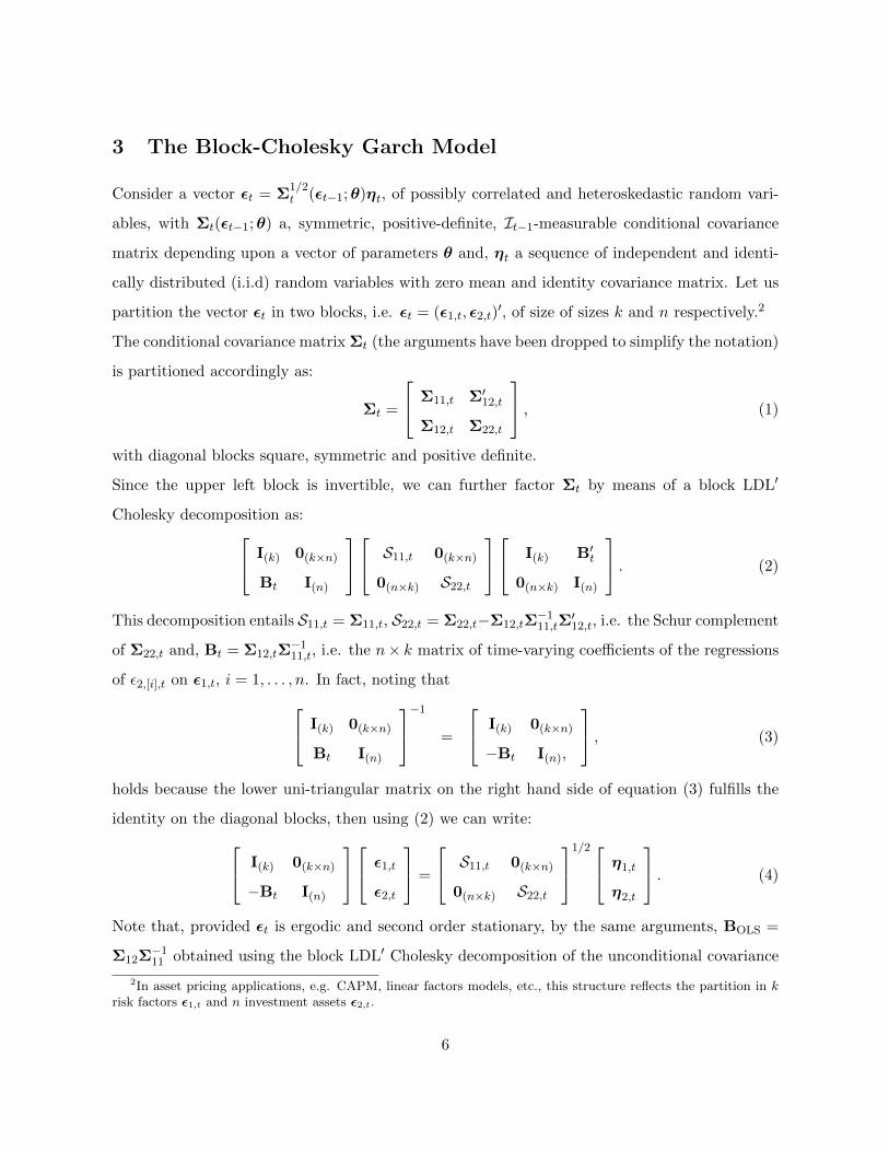
3 The Block-Cholesky Garch Model

Consider a vector εt = Σ1/2t (εt−1;θ)ηt, of possibly correlated and heteroskedastic random vari-

ables, with Σt(εt−1;θ) a, symmetric, positive-definite, It−1-measurable conditional covariance

matrix depending upon a vector of parameters θ and, ηt a sequence of independent and identi-

cally distributed (i.i.d) random variables with zero mean and identity covariance matrix. Let us

partition the vector εt in two blocks, i.e. εt = (ε1,t, ε2,t)′, of size of sizes k and n respectively.2

The conditional covariance matrix Σt (the arguments have been dropped to simplify the notation)

is partitioned accordingly as:

Σt =

Σ11,t Σ′12,t

Σ12,t Σ22,t

, (1)

with diagonal blocks square, symmetric and positive definite.

Since the upper left block is invertible, we can further factor Σt by means of a block LDL′

Cholesky decomposition as: I(k) 0(k×n)

Bt I(n)

S11,t 0(k×n)

0(n×k) S22,t

I(k) B′t

0(n×k) I(n)

. (2)

This decomposition entails S11,t = Σ11,t, S22,t = Σ22,t−Σ12,tΣ−111,tΣ

′12,t, i.e. the Schur complement

of Σ22,t and, Bt = Σ12,tΣ−111,t, i.e. the n× k matrix of time-varying coefficients of the regressions

of ε2,[i],t on ε1,t, i = 1, . . . , n. In fact, noting that I(k) 0(k×n)

Bt I(n)

−1

=

I(k) 0(k×n)

−Bt I(n),

, (3)

holds because the lower uni-triangular matrix on the right hand side of equation (3) fulfills the

identity on the diagonal blocks, then using (2) we can write: I(k) 0(k×n)

−Bt I(n)

ε1,t

ε2,t

=

S11,t 0(k×n)

0(n×k) S22,t

1/2 η1,t

η2,t

. (4)

Note that, provided εt is ergodic and second order stationary, by the same arguments, BOLS =

Σ12Σ−111 obtained using the block LDL′ Cholesky decomposition of the unconditional covariance

2In asset pricing applications, e.g. CAPM, linear factors models, etc., this structure reflects the partition in krisk factors ε1,t and n investment assets ε2,t.

6

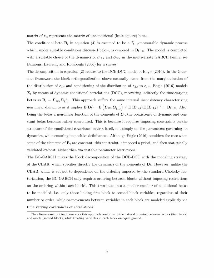
matrix of εt, represents the matrix of unconditional (least square) betas.

The conditional beta Bt in equation (4) is assumed to be a It−1-measurable dynamic process

which, under suitable conditions discussed below, is centered in BOLS. The model is completed

with a suitable choice of the dynamics of S11,t and S22,t in the multivariate GARCH family, see

Bauwens, Laurent, and Rombouts (2006) for a survey.

The decomposition in equation (2) relates to the DCB-DCC model of Engle (2016). In the Gaus-

sian framework the block orthogonalization above naturally stems from the marginalization of

the distribution of ε1,t and conditioning of the distribution of ε2,t to ε1,t. Engle (2016) models

Σt by means of dynamic conditional correlations (DCC), recovering indirectly the time-varying

betas as Bt = Σ12,tΣ−111,t. This approach suffers the same internal inconsistency characterizing

non linear dynamics as it implies E(Bt) = E(Σ12,tΣ

−111,t

)6= E (Σ12,t) E (Σ11,t)

−1 = BOLS. Also,

being the betas a non-linear function of the elements of Σt, the coexistence of dynamic and con-

stant betas becomes rather convoluted. This is because it requires imposing constraints on the

structure of the conditional covariance matrix itself, not simply on the parameters governing its

dynamics, while ensuring its positive definiteness. Although Engle (2016) considers the case when

some of the elements of Bt are constant, this constraint is imposed a priori, and then statistically

validated ex-post, rather then via testable parameter restrictions.

The BC-GARCH mixes the block decomposition of the DCB-DCC with the modeling strategy

of the CHAR, which specifies directly the dynamics of the elements of Bt. However, unlike the

CHAR, which is subject to dependence on the ordering imposed by the standard Cholesky fac-

torization, the BC-GARCH only requires ordering between blocks without imposing restrictions

on the ordering within each block3. This translates into a smaller number of conditional betas

to be modeled, i.e. only those linking first block to second block variables, regardless of their

number or order, while co-movements between variables in each block are modeled explicitly via

time varying covariances or correlations.

3In a linear asset pricing framework this approach conforms to the natural ordering between factors (first block)and assets (second block), while treating variables in each block on equal ground.

7

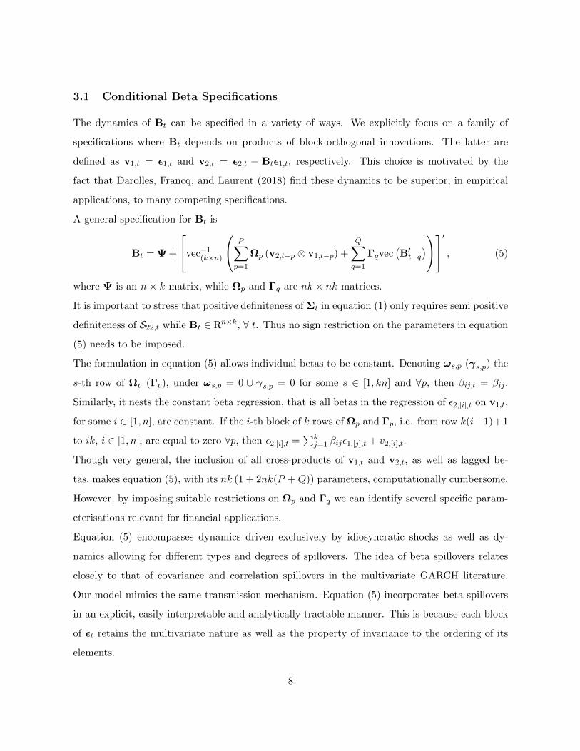
3.1 Conditional Beta Specifications

The dynamics of Bt can be specified in a variety of ways. We explicitly focus on a family of

specifications where Bt depends on products of block-orthogonal innovations. The latter are

defined as v1,t = ε1,t and v2,t = ε2,t − Btε1,t, respectively. This choice is motivated by the

fact that Darolles, Francq, and Laurent (2018) find these dynamics to be superior, in empirical

applications, to many competing specifications.

A general specification for Bt is

Bt = Ψ +

vec−1(k×n)

P∑p=1

Ωp (v2,t−p ⊗ v1,t−p) +

Q∑q=1

Γqvec(B′t−q

)′ , (5)

where Ψ is an n× k matrix, while Ωp and Γq are nk × nk matrices.

It is important to stress that positive definiteness of Σt in equation (1) only requires semi positive

definiteness of S22,t while Bt ∈ Rn×k, ∀ t. Thus no sign restriction on the parameters in equation

(5) needs to be imposed.

The formulation in equation (5) allows individual betas to be constant. Denoting ωs,p (γs,p) the

s-th row of Ωp (Γp), under ωs,p = 0 ∪ γs,p = 0 for some s ∈ [1, kn] and ∀p, then βij,t = βij .

Similarly, it nests the constant beta regression, that is all betas in the regression of ε2,[i],t on v1,t,

for some i ∈ [1, n], are constant. If the i-th block of k rows of Ωp and Γp, i.e. from row k(i−1)+1

to ik, i ∈ [1, n], are equal to zero ∀p, then ε2,[i],t =∑k

j=1 βijε1,[j],t + v2,[i],t.

Though very general, the inclusion of all cross-products of v1,t and v2,t, as well as lagged be-

tas, makes equation (5), with its nk (1 + 2nk(P +Q)) parameters, computationally cumbersome.

However, by imposing suitable restrictions on Ωp and Γq we can identify several specific param-

eterisations relevant for financial applications.

Equation (5) encompasses dynamics driven exclusively by idiosyncratic shocks as well as dy-

namics allowing for different types and degrees of spillovers. The idea of beta spillovers relates

closely to that of covariance and correlation spillovers in the multivariate GARCH literature.

Our model mimics the same transmission mechanism. Equation (5) incorporates beta spillovers

in an explicit, easily interpretable and analytically tractable manner. This is because each block

of εt retains the multivariate nature as well as the property of invariance to the ordering of its

elements.

8

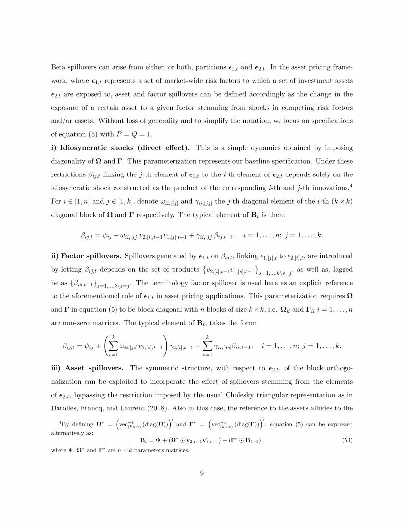
Beta spillovers can arise from either, or both, partitions ε1,t and ε2,t. In the asset pricing frame-

work, where ε1,t represents a set of market-wide risk factors to which a set of investment assets

ε2,t are exposed to, asset and factor spillovers can be defined accordingly as the change in the

exposure of a certain asset to a given factor stemming from shocks in competing risk factors

and/or assets. Without loss of generality and to simplify the notation, we focus on specifications

of equation (5) with P = Q = 1.

i) Idiosyncratic shocks (direct effect). This is a simple dynamics obtained by imposing

diagonality of Ω and Γ. This parameterization represents our baseline specification. Under these

restrictions βij,t linking the j-th element of ε1,t to the i-th element of ε2,t depends solely on the

idiosyncratic shock constructed as the product of the corresponding i-th and j-th innovations.4

For i ∈ [1, n] and j ∈ [1, k], denote ωii,[jj] and γii,[jj] the j-th diagonal element of the i-th (k× k)

diagonal block of Ω and Γ respectively. The typical element of Bt is then:

βij,t = ψij + ωii,[jj]v2,[i],t−1v1,[j],t−1 + γii,[jj]βij,t−1, i = 1, . . . , n; j = 1, . . . , k.

ii) Factor spillovers. Spillovers generated by ε1,t on βij,t, linking ε1,[j],t to ε2,[i],t, are introduced

by letting βij,t depends on the set of productsv2,[i],t−1v1,[s],t−1

s=1,...,k\s=j , as well as, lagged

betas βis,t−1s=1,...,k\s=j . The terminology factor spillover is used here as an explicit reference

to the aforementioned role of ε1,t in asset pricing applications. This parameterization requires Ω

and Γ in equation (5) to be block diagonal with n blocks of size k×k, i.e. Ωii and Γii i = 1, . . . , n

are non-zero matrices. The typical element of Bt, takes the form:

βij,t = ψij +

(k∑s=1

ωii,[js]v1,[s],t−1

)v2,[i],t−1 +

k∑s=1

γii,[js]βis,t−1, i = 1, . . . , n; j = 1, . . . , k.

iii) Asset spillovers. The symmetric structure, with respect to ε2,t, of the block orthogo-

nalization can be exploited to incorporate the effect of spillovers stemming from the elements

of ε2,t, bypassing the restriction imposed by the usual Cholesky triangular representation as in

Darolles, Francq, and Laurent (2018). Also in this case, the reference to the assets alludes to the

4By defining Ω∗ =(

vec−1(k×n) (diag(Ω))

)′and Γ∗ =

(vec−1

(k×n) (diag(Γ)))′

, equation (5) can be expressed

alternatively as:Bt = Ψ +

(Ω∗ v2,t−1v

′1,t−1

)+ (Γ∗ Bt−1) , (5.i)

where Ψ, Ω∗ and Γ∗ are n× k parameters matrices.

9

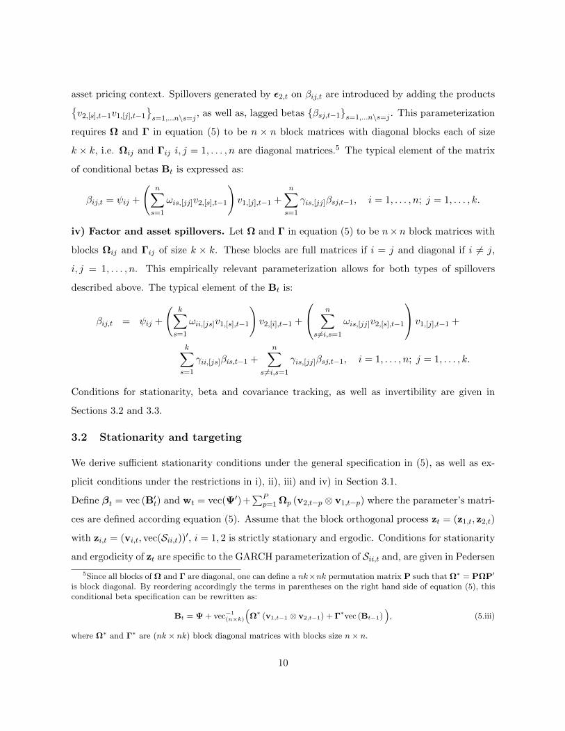
asset pricing context. Spillovers generated by ε2,t on βij,t are introduced by adding the productsv2,[s],t−1v1,[j],t−1

s=1,...n\s=j , as well as, lagged betas βsj,t−1s=1,...n\s=j . This parameterization

requires Ω and Γ in equation (5) to be n × n block matrices with diagonal blocks each of size

k × k, i.e. Ωij and Γij i, j = 1, . . . , n are diagonal matrices.5 The typical element of the matrix

of conditional betas Bt is expressed as:

βij,t = ψij +

(n∑s=1

ωis,[jj]v2,[s],t−1

)v1,[j],t−1 +

n∑s=1

γis,[jj]βsj,t−1, i = 1, . . . , n; j = 1, . . . , k.

iv) Factor and asset spillovers. Let Ω and Γ in equation (5) to be n×n block matrices with

blocks Ωij and Γij of size k × k. These blocks are full matrices if i = j and diagonal if i 6= j,

i, j = 1, . . . , n. This empirically relevant parameterization allows for both types of spillovers

described above. The typical element of the Bt is:

βij,t = ψij +

(k∑s=1

ωii,[js]v1,[s],t−1

)v2,[i],t−1 +

n∑s 6=i,s=1

ωis,[jj]v2,[s],t−1

v1,[j],t−1 +

k∑s=1

γii,[js]βis,t−1 +

n∑s 6=i,s=1

γis,[jj]βsj,t−1, i = 1, . . . , n; j = 1, . . . , k.

Conditions for stationarity, beta and covariance tracking, as well as invertibility are given in

Sections 3.2 and 3.3.

3.2 Stationarity and targeting

We derive sufficient stationarity conditions under the general specification in (5), as well as ex-

plicit conditions under the restrictions in i), ii), iii) and iv) in Section 3.1.

Define βt = vec (B′t) and wt = vec(Ψ′)+∑P

p=1 Ωp (v2,t−p ⊗ v1,t−p) where the parameter’s matri-

ces are defined according equation (5). Assume that the block orthogonal process zt = (z1,t, z2,t)

with zi,t = (vi,t, vec(Sii,t))′, i = 1, 2 is strictly stationary and ergodic. Conditions for stationarity

and ergodicity of zt are specific to the GARCH parameterization of Sii,t and, are given in Pedersen

5Since all blocks of Ω and Γ are diagonal, one can define a nk×nk permutation matrix P such that Ω∗ = PΩP′

is block diagonal. By reordering accordingly the terms in parentheses on the right hand side of equation (5), thisconditional beta specification can be rewritten as:

Bt = Ψ + vec−1(n×k)

(Ω∗ (v1,t−1 ⊗ v2,t−1) + Γ∗vec (Bt−1)

), (5.iii)

where Ω∗ and Γ∗ are (nk × nk) block diagonal matrices with blocks size n× n.

10

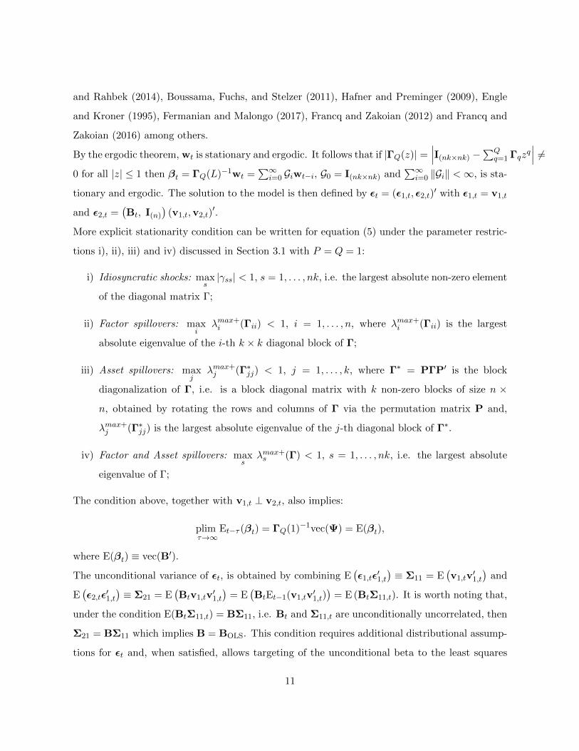
and Rahbek (2014), Boussama, Fuchs, and Stelzer (2011), Hafner and Preminger (2009), Engle

and Kroner (1995), Fermanian and Malongo (2017), Francq and Zakoian (2012) and Francq and

Zakoian (2016) among others.

By the ergodic theorem, wt is stationary and ergodic. It follows that if |ΓQ(z)| =∣∣∣I(nk×nk) −

∑Qq=1 Γqz

q∣∣∣ 6=

0 for all |z| ≤ 1 then βt = ΓQ(L)−1wt =∑∞

i=0 Giwt−i, G0 = I(nk×nk) and∑∞

i=0 ‖Gi‖ <∞, is sta-

tionary and ergodic. The solution to the model is then defined by εt = (ε1,t, ε2,t)′ with ε1,t = v1,t

and ε2,t =(Bt, I(n)

)(v1,t,v2,t)

′.

More explicit stationarity condition can be written for equation (5) under the parameter restric-

tions i), ii), iii) and iv) discussed in Section 3.1 with P = Q = 1:

i) Idiosyncratic shocks: maxs|γss| < 1, s = 1, . . . , nk, i.e. the largest absolute non-zero element

of the diagonal matrix Γ;

ii) Factor spillovers: maxi

λmax+i (Γii) < 1, i = 1, . . . , n, where λmax+

i (Γii) is the largest

absolute eigenvalue of the i-th k × k diagonal block of Γ;

iii) Asset spillovers: maxj

λmax+j (Γ∗jj) < 1, j = 1, . . . , k, where Γ∗ = PΓP′ is the block

diagonalization of Γ, i.e. is a block diagonal matrix with k non-zero blocks of size n ×

n, obtained by rotating the rows and columns of Γ via the permutation matrix P and,

λmax+j (Γ∗jj) is the largest absolute eigenvalue of the j-th diagonal block of Γ∗.

iv) Factor and Asset spillovers: maxs

λmax+s (Γ) < 1, s = 1, . . . , nk, i.e. the largest absolute

eigenvalue of Γ;

The condition above, together with v1,t ⊥ v2,t, also implies:

plimτ→∞

Et−τ (βt) = ΓQ(1)−1vec(Ψ) = E(βt),

where E(βt) ≡ vec(B′).

The unconditional variance of εt, is obtained by combining E(ε1,tε

′1,t

)≡ Σ11 = E

(v1,tv

′1,t

)and

E(ε2,tε

′1,t

)≡ Σ21 = E

(Btv1,tv

′1,t

)= E

(BtEt−1(v1,tv

′1,t))

= E (BtΣ11,t). It is worth noting that,

under the condition E(BtΣ11,t) = BΣ11, i.e. Bt and Σ11,t are unconditionally uncorrelated, then

Σ21 = BΣ11 which implies B = BOLS. This condition requires additional distributional assump-

tions for εt and, when satisfied, allows targeting of the unconditional beta to the least squares

11

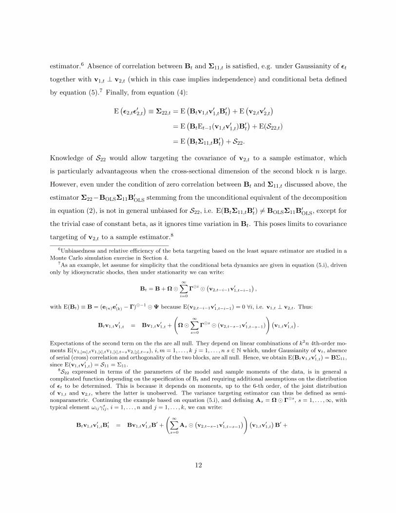
estimator.6 Absence of correlation between Bt and Σ11,t is satisfied, e.g. under Gaussianity of εt

together with v1,t ⊥ v2,t (which in this case implies independence) and conditional beta defined

by equation (5).7 Finally, from equation (4):

E(ε2,tε

′2,t

)≡ Σ22,t = E

(Btv1,tv

′1,tB

′t

)+ E

(v2,tv

′2,t

)= E

(BtEt−1(v1,tv

′1,t)B

′t

)+ E(S22,t)

= E(BtΣ11,tB

′t

)+ S22.

Knowledge of S22 would allow targeting the covariance of v2,t to a sample estimator, which

is particularly advantageous when the cross-sectional dimension of the second block n is large.

However, even under the condition of zero correlation between Bt and Σ11,t discussed above, the

estimator Σ22−BOLSΣ11B′OLS stemming from the unconditional equivalent of the decomposition

in equation (2), is not in general unbiased for S22, i.e. E(BtΣ11,tB′t) 6= BOLSΣ11B

′OLS, except for

the trivial case of constant beta, as it ignores time variation in Bt. This poses limits to covariance

targeting of v2,t to a sample estimator.8

6Unbiasedness and relative efficiency of the beta targeting based on the least square estimator are studied in aMonte Carlo simulation exercise in Section 4.

7As an example, let assume for simplicity that the conditional beta dynamics are given in equation (5.i), drivenonly by idiosyncratic shocks, then under stationarity we can write:

Bt = B + Ω∞∑i=0

Γi (v2,t−i−1v

′1,t−i−1

),

with E(Bt) ≡ B = (e(n)e′(k) − Γ)−1 Ψ because E(v2,t−i−1v

′1,t−i−1) = 0 ∀i, i.e. v1,t ⊥ v2,t. Thus:

Btv1,tv′1,t = Bv1,tv

′1,t +

(Ω

∞∑s=0

Γs (v2,t−s−1v′1,t−s−1)

)(v1,tv

′1,t

).

Expectations of the second term on the rhs are all null. They depend on linear combinations of k2n 4th-order mo-ments E(v1,[m],tv1,[i],tv1,[i],t−sv2,[j],t−s), i,m = 1, . . . , k j = 1, . . . , n s ∈ N which, under Gaussianity of vt, absenceof serial (cross) correlation and orthogonality of the two blocks, are all null. Hence, we obtain E(Btv1,tv

′1,t) = BΣ11,

since E(v1,tv′1,t) = S11 = Σ11.

8S22 expressed in terms of the parameters of the model and sample moments of the data, is in general acomplicated function depending on the specification of Bt and requiring additional assumptions on the distributionof εt to be determined. This is because it depends on moments, up to the 6-th order, of the joint distributionof v1,t and v2,t, where the latter is unobserved. The variance targeting estimator can thus be defined as semi-nonparametric. Continuing the example based on equation (5.i), and defining As = Ω Γs, s = 1, . . . ,∞, withtypical element ωijγ

sij , i = 1, . . . , n and j = 1, . . . , k, we can write:

Btv1,tv′1,tB

′t = Bv1,tv

′1,tB

′ +

(∞∑s=0

As (v2,t−s−1v

′1,t−s−1

)) (v1,tv

′1,t

)B′ +

12

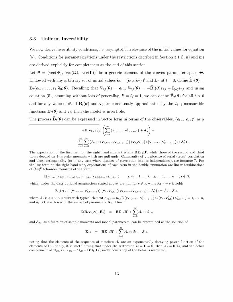
3.3 Uniform Invertibility

We now derive invertibility conditions, i.e. asymptotic irrelevance of the initial values for equation

(5). Conditions for parameterizations under the restrictions decribed in Section 3.1 i), ii) and iii)

are derived explicitly for completeness at the end of this section.

Let θ = (vec(Ψ), vec(Ω), vec(Γ))′ be a generic element of the convex parameter space Θ.

Endowed with any arbitrary set of initial values ε0 = (ε1,0, ε2,0)′ and B0 at t = 0, define Bt(θ) =

Bt(εt−1, . . . , ε1, ε0;θ). Recalling that v1,t(θ) = ε1,t, v2,t(θ) = −Bt(θ)ε1,t + I(n)ε2,t and using

equation (5), assuming without loss of generality, P = Q = 1, we can define Bt(θ) for all t > 0

and for any value of θ. If Bt(θ) and vt are consistently approximated by the It−1-measurable

functions Bt(θ) and vt, then the model is invertible.

The process Bt(θ) can be expressed in vector form in terms of the observables, (ε1,t, ε2,t)′, as a

+B(v1,tv′1,t)

(∞∑s=0

(v1,t−s−1v

′2,t−s−1

)A′s

)+

+

∞∑s=0

∞∑r=0

(As

(v2,t−s−1v

′1,t−s−1

)) (v1,tv

′1,t

) ((v1,t−r−1v

′2,t−r−1

)A′r

).

The expectation of the first term on the right hand side is trivially BΣ11B′, while those of the second and third

terms depend on 4-th order moments which are null under Gaussianity of vt, absence of serial (cross) correlationand block orthogonality (or in any case where absence of correlation implies independence), see footnote 7. Forthe last term on the right hand side, expectations of each term in the double summation are linear combinationsof (kn)2 6th-order moments of the form:

E(v1,[m],tv1,[i],tv1,[m],t−sv1,[i],t−rv2,[j],t−sv2,[l],t−r), i,m = 1, . . . , k j, l = 1, . . . , n r, s ∈ N,

which, under the distributional assumptions stated above, are null for r 6= s, while for r = s it holds

E((

As (v2,t−s−1v

′1,t−s−1

)) (v1,tv

′1,t

) ((v1,t−s−1v

′2,t−s−1

)A′s

))= As S22,

where As is a n× n matrix with typical element αij,s = ai,sE((v1,t−s−1v

′1,t−s−1) (v1,tv

′1,t))a′j,s, i, j = 1, . . . , n,

and ai is the i-th row of the matrix of parameters As. Thus:

E(Btv1,tv′1,tB

′t) = BΣ11B

′ +

∞∑s=0

As S22,

and S22, as a function of sample moments and model parameters, can be determined as the solution of

Σ22 = BΣ11B′ +

∞∑s=0

As S22 + S22,

noting that the elements of the sequence of matrices As are an exponentially decaying power function of theelements of Γ. Finally, it is worth noting that under the restriction Ω = Γ = 0, then As = 0 ∀s, and the Schurcomplement of Σ22, i.e. S22 = Σ22 −BΣ11B

′, under constancy of the betas is recovered.

13

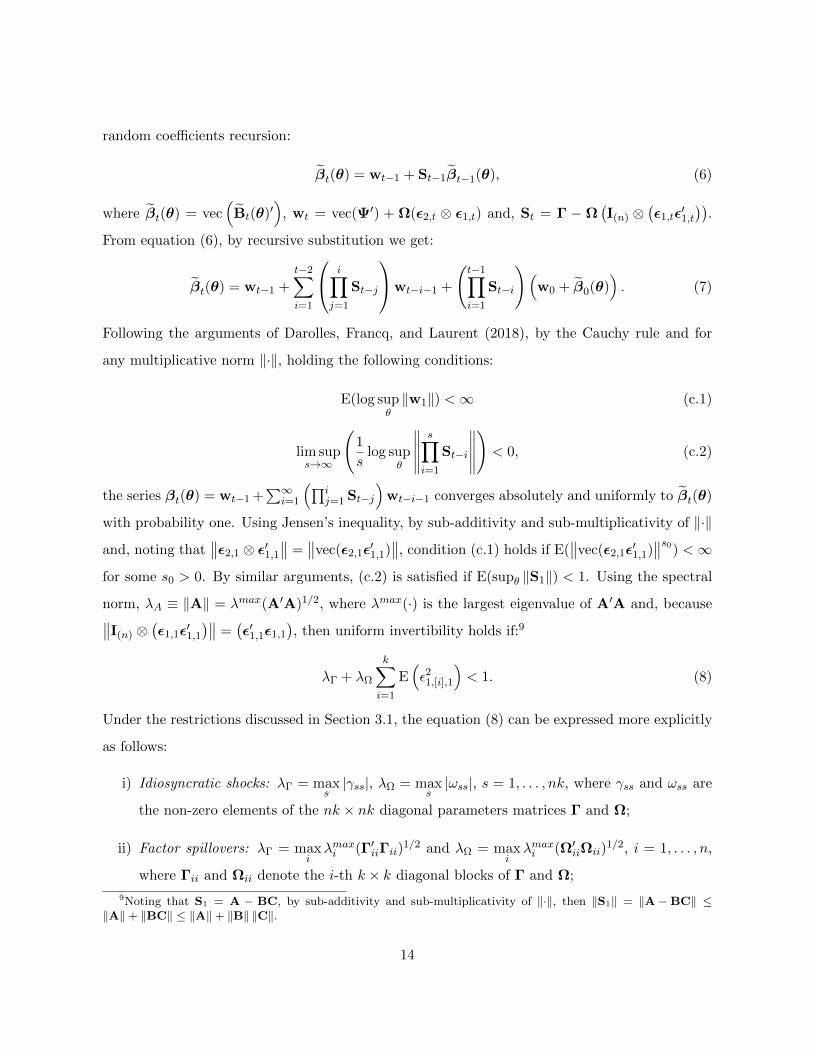
random coefficients recursion:

βt(θ) = wt−1 + St−1βt−1(θ), (6)

where βt(θ) = vec(Bt(θ)′

), wt = vec(Ψ′) + Ω(ε2,t ⊗ ε1,t) and, St = Γ − Ω

(I(n) ⊗

(ε1,tε

′1,t

)).

From equation (6), by recursive substitution we get:

βt(θ) = wt−1 +

t−2∑i=1

i∏j=1

St−j

wt−i−1 +

(t−1∏i=1

St−i

)(w0 + β0(θ)

). (7)

Following the arguments of Darolles, Francq, and Laurent (2018), by the Cauchy rule and for

any multiplicative norm ‖·‖, holding the following conditions:

E(log supθ‖w1‖) <∞ (c.1)

lim sups→∞

(1

slog sup

θ

∥∥∥∥∥s∏i=1

St−i

∥∥∥∥∥)< 0, (c.2)

the series βt(θ) = wt−1 +∑∞

i=1

(∏ij=1 St−j

)wt−i−1 converges absolutely and uniformly to βt(θ)

with probability one. Using Jensen’s inequality, by sub-additivity and sub-multiplicativity of ‖·‖

and, noting that∥∥ε2,1 ⊗ ε′1,1

∥∥ =∥∥vec(ε2,1ε

′1,1)∥∥, condition (c.1) holds if E(

∥∥vec(ε2,1ε′1,1)∥∥s0) <∞

for some s0 > 0. By similar arguments, (c.2) is satisfied if E(supθ ‖S1‖) < 1. Using the spectral

norm, λA ≡ ‖A‖ = λmax(A′A)1/2, where λmax(·) is the largest eigenvalue of A′A and, because∥∥I(n) ⊗(ε1,1ε

′1,1

)∥∥ =(ε′1,1ε1,1

), then uniform invertibility holds if:9

λΓ + λΩ

k∑i=1

E(ε21,[i],1

)< 1. (8)

Under the restrictions discussed in Section 3.1, the equation (8) can be expressed more explicitly

as follows:

i) Idiosyncratic shocks: λΓ = maxs|γss|, λΩ = max

s|ωss|, s = 1, . . . , nk, where γss and ωss are

the non-zero elements of the nk × nk diagonal parameters matrices Γ and Ω;

ii) Factor spillovers: λΓ = maxiλmaxi (Γ′iiΓii)

1/2 and λΩ = maxiλmaxi (Ω′iiΩii)

1/2, i = 1, . . . , n,

where Γii and Ωii denote the i-th k × k diagonal blocks of Γ and Ω;

9Noting that S1 = A − BC, by sub-additivity and sub-multiplicativity of ‖·‖, then ‖S1‖ = ‖A−BC‖ ≤‖A‖+ ‖BC‖ ≤ ‖A‖+ ‖B‖ ‖C‖.

14

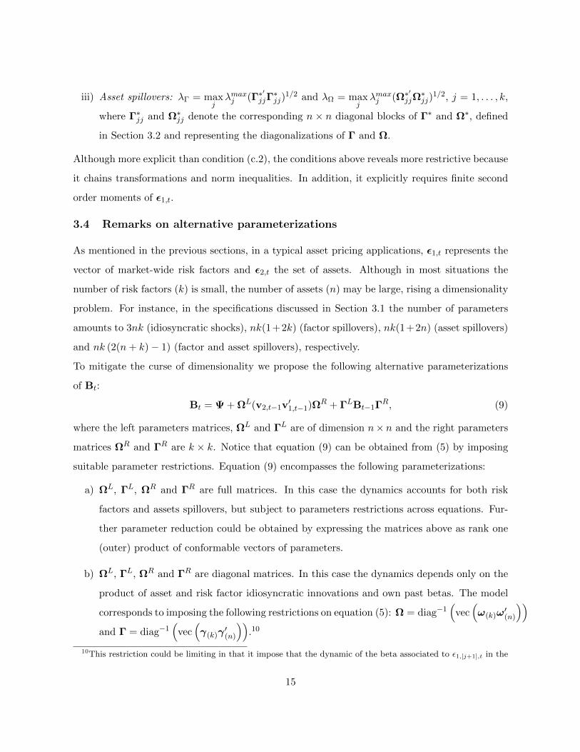
iii) Asset spillovers: λΓ = maxjλmaxj (Γ∗

′jjΓ∗jj)

1/2 and λΩ = maxjλmaxj (Ω∗

′jjΩ

∗jj)

1/2, j = 1, . . . , k,

where Γ∗jj and Ω∗jj denote the corresponding n × n diagonal blocks of Γ∗ and Ω∗, defined

in Section 3.2 and representing the diagonalizations of Γ and Ω.

Although more explicit than condition (c.2), the conditions above reveals more restrictive because

it chains transformations and norm inequalities. In addition, it explicitly requires finite second

order moments of ε1,t.

3.4 Remarks on alternative parameterizations

As mentioned in the previous sections, in a typical asset pricing applications, ε1,t represents the

vector of market-wide risk factors and ε2,t the set of assets. Although in most situations the

number of risk factors (k) is small, the number of assets (n) may be large, rising a dimensionality

problem. For instance, in the specifications discussed in Section 3.1 the number of parameters

amounts to 3nk (idiosyncratic shocks), nk(1+2k) (factor spillovers), nk(1+2n) (asset spillovers)

and nk (2(n+ k)− 1) (factor and asset spillovers), respectively.

To mitigate the curse of dimensionality we propose the following alternative parameterizations

of Bt:

Bt = Ψ + ΩL(v2,t−1v′1,t−1)ΩR + ΓLBt−1Γ

R, (9)

where the left parameters matrices, ΩL and ΓL are of dimension n× n and the right parameters

matrices ΩR and ΓR are k × k. Notice that equation (9) can be obtained from (5) by imposing

suitable parameter restrictions. Equation (9) encompasses the following parameterizations:

a) ΩL, ΓL, ΩR and ΓR are full matrices. In this case the dynamics accounts for both risk

factors and assets spillovers, but subject to parameters restrictions across equations. Fur-

ther parameter reduction could be obtained by expressing the matrices above as rank one

(outer) product of conformable vectors of parameters.

b) ΩL, ΓL, ΩR and ΓR are diagonal matrices. In this case the dynamics depends only on the

product of asset and risk factor idiosyncratic innovations and own past betas. The model

corresponds to imposing the following restrictions on equation (5): Ω = diag−1(

vec(ω(k)ω

′(n)

))and Γ = diag−1

(vec(γ(k)γ

′(n)

)).10

10This restriction could be limiting in that it impose that the dynamic of the beta associated to ε1,[j+1],t in the

15

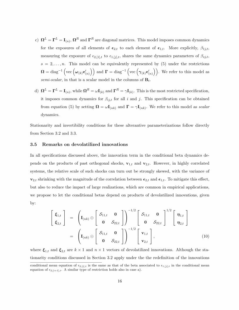
c) ΩL = ΓL = I(n), ΩR and ΓR are diagonal matrices. This model imposes common dynamics

for the exposures of all elements of ε2,t to each element of ε1,t. More explicitly, β1j,t,

measuring the exposure of ε2,[1],t to ε1,[j],t, shares the same dynamics parameters of βsj,t,

s = 2, . . . , n. This model can be equivalently represented by (5) under the restrictions

Ω = diag−1(

vec(ω(k)e

′(n)

))and Γ = diag−1

(vec(γ(k)e

′(n)

)). We refer to this model as

semi-scalar, in that is a scalar model in the columns of Bt.

d) ΩL = ΓL = I(n), while ΩR = ωI(k) and ΓR = γI(k). This is the most restricted specification,

it imposes common dynamics for βij,t for all i and j. This specification can be obtained

from equation (5) by setting Ω = ωI(nk) and Γ = γI(nk). We refer to this model as scalar

dynamics.

Stationarity and invertibility conditions for these alterantive parameterizations follow directly

from Section 3.2 and 3.3.

3.5 Remarks on devolatilized innovations

In all specifications discussed above, the innovation term in the conditional beta dynamics de-

pends on the products of past orthogonal shocks, v1,t and v2,t. However, in highly correlated

systems, the relative scale of such shocks can turn out be strongly skewed, with the variance of

v2,t shrinking with the magnitude of the correlation between ε2,t and ε1,t. To mitigate this effect,

but also to reduce the impact of large realizations, which are common in empirical applications,

we propose to let the conditional betas depend on products of devolatilized innovations, given

by: ξ1,t

ξ2,t

=

I(nk)

S11,t 0

0 S22,t

−1/2 S11,t 0

0 S22,t

1/2 η1,t

η2,t

=

I(nk)

S11,t 0

0 S22,t

−1/2 v1,t

v2,t

, (10)

where ξ1,t and ξ2,t are k × 1 and n × 1 vectors of devolatilized innovations. Although the sta-

tionarity conditions discussed in Section 3.2 apply under the the redefinition of the innovations

conditional mean equation of ε2,[i],t is the same as that of the beta associated to ε1,[j],t in the conditional meanequation of ε2,[i+1],t. A similar type of restriction holds also in case a).

16

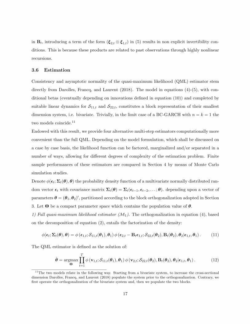
in Bt, introducing a term of the form (ξ2,t ⊗ ξ1,t) in (5) results in non explicit invertibility con-

ditions. This is because these products are related to past observations through highly nonlinear

recursions.

3.6 Estimation

Consistency and asymptotic normality of the quasi-maximum likelihood (QML) estimator stem

directly from Darolles, Francq, and Laurent (2018). The model in equations (4)-(5), with con-

ditional betas (eventually depending on innovations defined in equation (10)) and completed by

suitable linear dynamics for S11,t and S22,t, constitutes a block representation of their smallest

dimension system, i.e. bivariate. Trivially, in the limit case of a BC-GARCH with n = k = 1 the

two models coincide.11

Endowed with this result, we provide four alternative multi-step estimators computationally more

convenient than the full QML. Depending on the model formulation, which shall be discussed on

a case by case basis, the likelihood function can be factored, marginalized and/or separated in a

number of ways, allowing for different degrees of complexity of the estimation problem. Finite

sample performances of these estimators are compared in Section 4 by means of Monte Carlo

simulation studies.

Denote φ(εt; Σt(θ),θ) the probability density function of a multivariate normally distributed ran-

dom vector εt with covariance matrix Σt(θ) = Σt(εt−1, εt−2, . . . ;θ). depending upon a vector of

parameters θ = (θ1,θ2)′, partitioned according to the block orthogonalization adopted in Section

3. Let Θ be a compact parameter space which contains the population value of θ.

1) Full quasi-maximum likelihood estimator (M1). The orthogonalization in equation (4), based

on the decomposition of equation (2), entails the factorization of the density:

φ(εt; Σt(θ),θ) = φ (ε1,t;S11,t(θ1),θ1)φ (ε2,t −Btε1,t;S22,t(θ2),Bt(θ2),θ2|ε1,t,θ1) . (11)

The QML estimator is defined as the solution of:

θ = argmaxΘ

T∏t=1

φ (v1,t;S11,t(θ1),θ1)φ (v2,t;S22,t(θ2),Bt(θ2),θ2|ε1,t,θ1) . (12)

11The two models relate in the following way. Starting from a bivariate system, to increase the cross-sectionaldimension Darolles, Francq, and Laurent (2018) populate the system prior to the orthogonalization. Contrary, wefirst operate the orthogonalization of the bivariate system and, then we populate the two blocks.

17

2) Two-step block-by-block estimator (M2). The two step-estimator of equations (4)-(5) exploits

the factorization in equation (11). Provided that S11,t(θ1) = S11,t(v1,t−1,v1,t−2, . . . ;θ1), such

that ∂S11,t/∂θ2 = 0 and similarly that ∂S22,t/∂θ1 = 0, then the two-step estimator, given by:

θ1 = argmaxΘ

T∏t=1

φ (v1,t;S11,t(θ1),θ1) , (13)

θ2 = argmaxΘ

T∏t=1

φ (v2,t;S22,t(θ2),Bt(θ2),θ2|ε1,t,θ1) . (14)

coincides with that of M1.12 However, if we let Bt depend on devolatilized innovations, defined

in equation (10), then ∂Bt/∂θ1 6= 0 and the two estimators will be different13, with the M1

estimator being in general more efficient.14

The following three approaches are based on further decomposition of the likelihood function

inspired by Francq and Zakoian (2016). They are appealing when the correlations implied by

S11,t and S22,t are not directly of interest and can be treated as nuisance parameters. This largely

reduces the dimension of the parameter space, increasing computational feasibility in large cross-

sectional dimensions n. Alternatively, these approaches can be seen as multi-step estimators

where, first, conditional means and variances are estimated (jointly or individually), and then,

conditioned on the previous steps, correlations are estimated by means of a Gaussian copula.15 It

is important to point out that these approaches, to different extents, limit the type of dynamics

that can be assumed for S11,t, S22,t and Bt in terms of cross-sectional interactions and constraints.

Let us denote C(ξs,t; Rs,t(θRs ),θR

s ), s = 1, 2, a Gaussian copula, with ξs,t defined in equation (10),

Rs,t(θRs ) the conditional correlation, implied by Sss,t, depending on parameters θR

s ∈ Θ. Also,

let us denote bj,t j = 1, . . . , n the j-th row of the matrix of conditional betas Bt. Finally, let us

denote θ−s the subset of parameters of the marginal distributions of vs,t, such that θs = θ−s ∪θR1 .

12The parameters of the second block can be estimated without any knowledge of the parameters of the firstblock, because Bt as defined in equation (5) depends on v1,t which is observed.

13Notice that this is also the case when Bt follows the dynamics in equation (5), but the model for S22,t is suchthat ∂S22,t/∂θ1 6= 0.

14Examples in a simplified setup can be found in Darolles, Francq, and Laurent (2018).15This approach can be cast in the constant/dynamic conditional correlation framework of Bollerslev (1990) and

Engle (2002), where the logarithmic transformation of C(ξs,t; Rs,t(θRs ),θR

s ) equals

−1

2

[log |Rs,t(θ

Rs )|+ ξ′s,t

(Rs,t(θ

Rs )−1 − I(n)

)ξs,t

].

18

The joint density can be written as:

φ(εt; Σt(θ),θ) =

(k∏i=1

φ(v1,[i],t;S11,[ii],t(θ

−1 ),θ−1

))C(ξ1,t; R1,t(θ

R1 ),θR

1

)× n∏

j=1

φ(v2,[j],t;S22,[jj],t(θ

−2 ),bj,t(θ

−2 ),θ−2 |v1,t,θ

−1

)C(ξ2,t; R2,t(θ

R2 ),θR

2

). .(15)

Note that the factorization above assumes that φ(v2,[j],t;S22,[jj],t(θ

−2 ),bj,t(θ

−2 ),θ−2 |v1,t,θ

−1

), i.e.

the marginal distribution of v2,[j],t, j = 1, . . . , n, depends only on the parameters of the marginal

distributions of v1,[i],t, i = 1, . . . , k, and not on θR1 .16

3) Joint maximization of marginal distributions (M3). When the correlation parameters are not

of interest, the problem can be reduced to:

θ−

= argmaxΘ

T∏t=1

k∏i=1

φ(v1,[i],t;S11,[ii],t(θ

−1 ),θ−1

) n∏j=1

φ(v2,[j],t;S22,[jj],t(θ

−2

),bj,t(θ

−2 ),θ−2 |v1,t,θ

−1 ),

(16)

where θ− denotes a reduced dimension parameter vector with respect to θ.

4) Two-step estimation based on block-by-block joint maximization of marginals (M4). Provided

that the conditions on S11,t, S22,t and Bt discussed in M2 are satisfied, then we can define:

θ−1 = argmax

Θ

T∏t=1

k∏i=1

φ(v1,[i],t;S11,[ii],t(θ

−1

),θ−1 ) (17)

θ−2 = argmax

Θ

T∏t=1

n∏j=1

φ(v2,[j],t;S22,[jj],t(θ

−2

),bj,t(θ

−2 ),θ−2 |v1,t,θ

−1 ). (18)

As previously discussed, M4 is equivalent to M3 whenever ∂Bt/∂θ1 = 0. It will differ when Bt

depends on devolatilized innovations, in general entailing a loss of efficiency.

5) Estimation equation-by-equation via marginal distributions (M5). This method relies upon the

maximal level of separation of the likelihood. It splits the maximization problem in kn individual

optimizations:

θ−i =

argmaxΘ

∏Tt=1 φ

(vi,t; ςi,t(θ

−i ),θ−i

), i = 1, . . . , k

argmaxΘ

∏Tt=1 φ

(vi,t; ςi,t(θ

−i ),bi−k,t(θ

−i ),θ−i |v1,t,θ

−1

), i = k + 1, . . . , k + n,

(19)

16This assumption allows for a reduction of the complexity of the estimation problem or a reduction of theparameter space without imposing limiting parameter constraints.

19

where vi,t is the i-th element of the kn × 1 vector vt = (v1,t,v2,t)′ and ςi,t is the i-th element

of (diag(S11,t), diag(S22,t))′. This method is the most computationally efficient in large cross-

sectional dimensions. By breaking the estimation in smaller problems it reduces the parameter

space and avoids the inversion of large dimension matrices.

To be feasible, this approach requires that the dynamics of S11,t, S22,t and Bt entail minimal or no

cross-sectional parameter restrictions or interactions between elements. For instance, conditional

betas driven by idiosyncratic shocks or factor spillovers can be accommodated, while dynamics

allowing for asset spillovers cannot.17 Similar arguments hold for the conditional covariance

matrices S11,t and S22,t.

As mentioned earlier,M3 toM5 can be used as a preliminary step prior to the estimation of the

conditional covariances (or correlations) implied by S11,t and S22,t. The off-diagonal elements of

S11,t and S22,t can be obtained by filtering, e.g. if Sii,t is a scalar or diagonal BEKK, or they can

be estimated, by means of a constant or dynamic correlation model, see Bollerslev (1990), Engle

(2002) and Aielli (2013) among others.

It is also worth noting that, despite covariance targeting being unfeasible in general for S22,t,

knowledge of diag(S22), allows targeting its off-diagonal elements by means of sample estimators

using first step residuals, e.g. S22,[ij] = T−1∑T

t=1 v2,[i],tv2,[j],t, i, j = 1, . . . , n and i 6= j. Although

these methods reduce the number of parameters18 and the complexity of the estimation,19 they

come at the cost of a loss of efficiency. This point will be addressed in detail in Section 4 by

means of a Monte Carlo simulation study.

4 Monte Carlo study

The finite sample performance of the Gaussian maximum likelihood estimator is evaluated by

means of two Monte Carlo exercise. The model setup is the following.

17When Bt depends on devolatilized innovations, the estimation of the parameters of the marginal distributionsof ε2,[j],t j = 1, . . . , n requires knowledge of S11,[ii],t, i = 1, . . . , k which need to be estimated first, imposingsequentiality of the estimation between the two blocks (but not within).

18In the most parsimonious specification the number of parameters of multivariate GARCH is of order O(n2),which reduces to O(n) in the case of separability and to O(1) in the case of marginalization, where n is thedimension of the system being modeled.

19While the computation of the full likelihood requires inverting covariance matrices, that of likelihood underseparability and marginalization requires computing only (scalar) fractions and sums.

20

The cross-sectional dimension of the system is set to five, with dimensions of the blocks k = 3

and n = 2 respectively. The sample sizes are T = 3750, 7500, 15000.

The model specification is given by equation (4) with ηt ∼ i.i.d N(0(5), I(5)). The matrix of

conditional betas Bt follows the simple dynamics driven by idiosyncratic shocks expressed as

in equation (5.i). The intercept term is reparameterized using the unconditional beta, Ψ =

B (e(2)e′

(3) − Γ). To assess the use of devolatilized shocks, the driving innovation in the

conditional betas depends on (ξ1,t, ξ2,t)′ defined in equation (10). The dynamics of Bt is thus

expressed as:

Bt = B (e(2)e′

(3) − Γ) + (Ω ξ2,t−1ξ′1,t−1) + (ΓBt−1). (20)

The 2× 3 matrices of parameters B, Ω and Γ, are set as follows:

B =

1.00 0.50 0.70

1.00 −0.50 0.00

, ωij = 0.04, γij = 0.95, ∀ i = 1, 2 and j = 1, 2, 3.

Although, this parameterization implies that all betas share common dynamics, the 2kn elements

of Ω and Γ are estimated individually, without imposing equality restrictions. Note that for β23,t,

the dynamics above together with β23 = 0 imply that ε2,[2],t and ε1,[3],t are conditionally correlated

but unconditionally orthogonal.

The model is completed by scalar BEKK dynamics for S11,t and S22,t, with intercept reparame-

terized via covariance tracking:

Sii,t = Sii(1− τi − δi) + τi(vi,tv′i,t) + δiSii,t−1, i = 1, 2, (21)

with parameters

S11 =

1.00 0.10 −0.10

0.10 1.00 0.10

−0.10 0.10 1.00

, S22 =

1.00 0.50

0.50 1.00

, τi = 0.04, δi = 0.95, i = 1, 2.

21

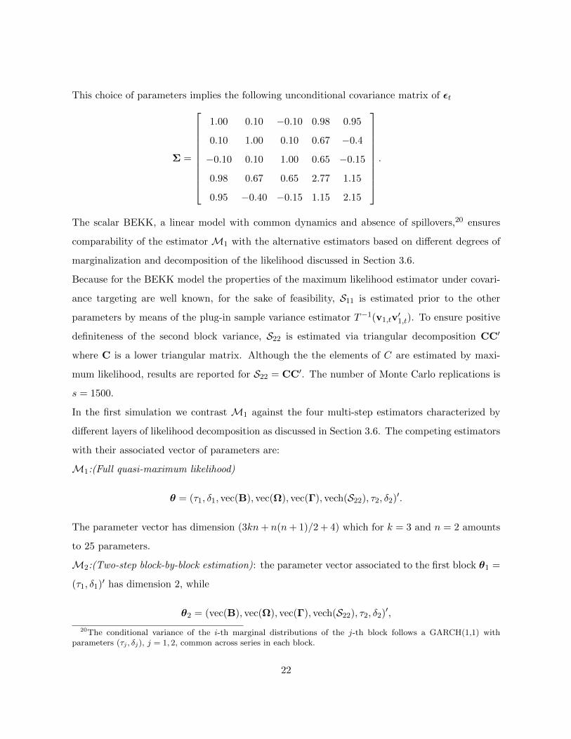
This choice of parameters implies the following unconditional covariance matrix of εt

Σ =

1.00 0.10 −0.10 0.98 0.95

0.10 1.00 0.10 0.67 −0.4

−0.10 0.10 1.00 0.65 −0.15

0.98 0.67 0.65 2.77 1.15

0.95 −0.40 −0.15 1.15 2.15

.

The scalar BEKK, a linear model with common dynamics and absence of spillovers,20 ensures

comparability of the estimator M1 with the alternative estimators based on different degrees of

marginalization and decomposition of the likelihood discussed in Section 3.6.

Because for the BEKK model the properties of the maximum likelihood estimator under covari-

ance targeting are well known, for the sake of feasibility, S11 is estimated prior to the other

parameters by means of the plug-in sample variance estimator T−1(v1,tv′1,t). To ensure positive

definiteness of the second block variance, S22 is estimated via triangular decomposition CC′

where C is a lower triangular matrix. Although the the elements of C are estimated by maxi-

mum likelihood, results are reported for S22 = CC′. The number of Monte Carlo replications is

s = 1500.

In the first simulation we contrast M1 against the four multi-step estimators characterized by

different layers of likelihood decomposition as discussed in Section 3.6. The competing estimators

with their associated vector of parameters are:

M1:(Full quasi-maximum likelihood)

θ = (τ1, δ1, vec(B), vec(Ω), vec(Γ), vech(S22), τ2, δ2)′.

The parameter vector has dimension (3kn+ n(n+ 1)/2 + 4) which for k = 3 and n = 2 amounts

to 25 parameters.

M2:(Two-step block-by-block estimation): the parameter vector associated to the first block θ1 =

(τ1, δ1)′ has dimension 2, while

θ2 = (vec(B), vec(Ω), vec(Γ), vech(S22), τ2, δ2)′,

20The conditional variance of the i-th marginal distributions of the j-th block follows a GARCH(1,1) withparameters (τj , δj), j = 1, 2, common across series in each block.

22

which denotes the second block parameters, has dimension 3kn + n(n + 1)/2 + 2. In our setup

the latter amounts to 23 parameters.

M3:(joint maximization of marginal distributions):

θ− = (τ1, δ1, vec(B), vec(Ω), vec(Γ), diag(S22), τ2, δ2)′.

The parameter vector has dimension (3k+1)n+4, which in our setup amounts to 24 parameters.

M4:(Two-step estimation based on block-by-block joint maximization of marginals): the first

block parameter vector is θ−1 = (τ1, δ1)′, while that of the second block is:

θ−2 = vec(B), vec(Ω), vec(Γ), diag(S22), τ2, δ2)′,

and has dimension (3k + 1)n + 2, which in our setup amounts to 22 parameters. Note that in

M3 and M4 the equality restriction on the parameters governing the dynamics of the marginal

variances S11,[ii],t i = 1, . . . , k and S22,[jj],t j = 1, . . . , n, is binding.

M5:(Estimation equation-by-equation via marginal distributions) the parameter vector θ−i equals

to:

θ−i =

(τ1,i, δ1,i)′ i = 1, . . . , k,

(bi−k,ωi−k,γi−k, ςii, τ2,i, δ2,i)′ i = k + 1, . . . , k + n.

Note that for i > k the dimension of θ−i is (3k + 3), in our case 12 parameters for each marginal

distribution of the second block. The total number of parameters is 30, which entails some re-

dundancy due to the fact that this estimation approach does not impose a priori the equality

restrictions on the parameters of the marginal variances, i.e. (τ1,i, δ1,i)′ = (τ1, δ1)′, i = 1, . . . , k

and similarly (τ2,j , δ2,j)′ = (τ2, δ2)′, j = 1, . . . , n.

For M3, M4 and M5 to be feasible and comparable to M1 and M2, the model must allow for

separability of the likelihood. This is the case in our setting because of the absence of volatil-

ity/covariance and, beta spillovers.

Table 1 reports the the Monte Carlo results. To save space, element-wise Bias and Root Mean

Squared Error (RMSE) for the first block plug-in estimator of the unconditional covariance S11,

common to all simulations in this section, are reported only once in the top portion of Table 2.

Due to the large number of parameters, we report average empirical bias and the square root of

the average mean squared error across the number of conditional betas (kn = 6) for the elements

23

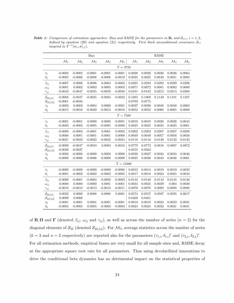
Table 1: Comparison of estimation approaches: Bias and RMSE for the parameters in Bt and Sii,t, i = 1, 2,defined by equation (20) and equation (21) respectively. First block unconditional covariance S11targeted to T−1(v1,tv

′1,t).

Bias RMSE

M1 M2 M3 M4 M5 M1 M2 M3 M4 M5

T = 3750

τ1 -0.0002 -0.0002 -0.0001 -0.0001 -0.0001 0.0026 0.0026 0.0036 0.0036 0.0064δ1 -0.0005 -0.0006 -0.0008 -0.0008 -0.0019 0.0035 0.0035 0.0049 0.0051 0.0092

βij 0.0007 0.0006 0.0006 0.0004 -0.0003 0.0285 0.0283 0.0292 0.0299 0.0296ωij 0.0001 0.0002 0.0003 0.0005 0.0003 0.0071 0.0072 0.0081 0.0082 0.0080γij -0.0043 -0.0047 -0.0055 -0.0058 -0.0050 0.0181 0.0183 0.0212 0.0214 0.0208

S22,[ii] -0.0068 -0.0047 -0.0025 -0.0004 -0.0023 0.1085 0.1069 0.1149 0.1181 0.1237

S22,[12] -0.0061 -0.0034 0.0793 0.0775

τ2 0.0003 0.0003 0.0004 0.0000 -0.0001 0.0037 0.0036 0.0048 0.0048 0.0063δ2 -0.0015 -0.0016 -0.0020 -0.0013 -0.0018 0.0052 0.0052 0.0068 0.0065 0.0088

T = 7500

τ1 -0.0001 -0.0001 0.0000 0.0000 -0.0001 0.0019 0.0019 0.0026 0.0026 0.0044δ1 -0.0003 -0.0003 -0.0005 -0.0005 -0.0009 0.0025 0.0025 0.0034 0.0035 0.0061

βij -0.0000 -0.0003 -0.0001 0.0001 0.0002 0.0202 0.0203 0.0207 0.0207 0.0209ωij 0.0000 0.0001 -0.0001 0.0001 0.0000 0.0049 0.0049 0.0057 0.0056 0.0056γij -0.0021 -0.0023 -0.0022 -0.0022 -0.0024 0.0116 0.0116 0.0130 0.0132 0.0132

S22,[ii] -0.0009 -0.0047 -0.0010 0.0003 -0.0016 0.0779 0.0773 0.0818 0.0807 0.0872

S22,[12] -0.0020 -0.0037 0.0555 0.0563

τ2 0.0002 -0.0000 -0.0000 0.0002 0.0000 0.0026 0.0027 0.0034 0.0034 0.0046δ2 -0.0008 -0.0006 -0.0006 -0.0008 -0.0009 0.0035 0.0036 0.0043 0.0046 0.0061

T = 15000

τ1 -0.0000 -0.0000 -0.0000 -0.0000 -0.0000 0.0013 0.0014 0.0019 0.0019 0.0032δ1 -0.0001 -0.0002 -0.0002 -0.0002 -0.0005 0.0017 0.0018 0.0024 0.0025 0.0043

βij -0.0000 -0.0001 -0.0004 -0.0002 -0.0003 0.0142 0.0140 0.0144 0.0145 0.0146ωij 0.0000 0.0000 0.0000 0.0001 0.0001 0.0034 0.0035 0.0039 0.004 0.0039γij -0.0010 -0.0010 -0.0013 -0.0013 -0.0011 0.0076 0.0076 0.0092 0.0088 0.0088

S22,[ii] 0.0022 0.0000 0.0008 0.0008 0.0001 0.0574 0.0557 0.0597 0.0595 0.0617

S22,[12] 0.0009 0.0008 0.0408 0.0401

τ2 0.0001 0.0001 0.0001 -0.0001 -0.0001 0.0018 0.0019 0.0024 0.0023 0.0031δ2 -0.0004 -0.0005 -0.0005 -0.0003 -0.0004 0.0024 0.0024 0.0032 0.0031 0.0041

of B,Ω and Γ (denoted βij , ωij and γij), as well as across the number of series (n = 2) for the

diagonal elements of S22 (denoted S22,[ii]). ForM5, average statistics across the number of series

(k = 3 and n = 2 respectively) are reported also for the parameters (τ1,i, δ1,i)′ and (τ2,j , δ2,j)

′.

For all estimation methods, empirical biases are very small for all sample sizes and, RMSE decay

at the appropriate square root rate for all parameters. Thus using devolatilized innovations to

drive the conditional beta dynamics has no detrimental impact on the statistical properties of

24

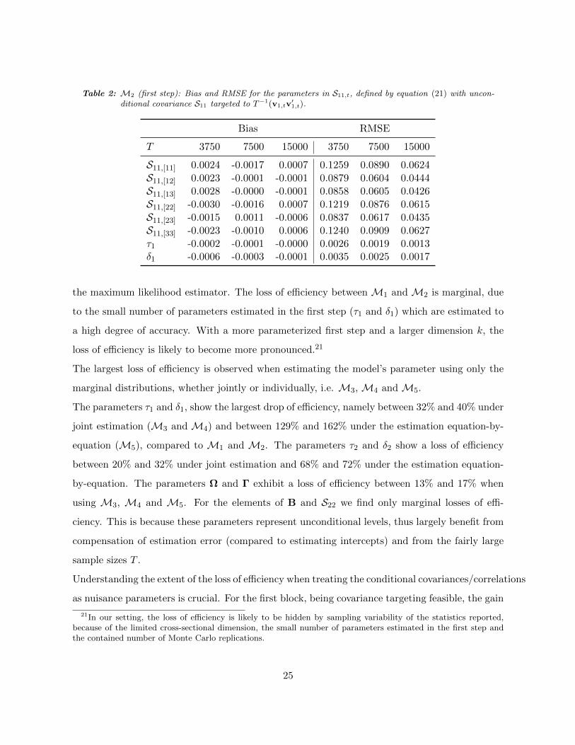
Table 2: M2 (first step): Bias and RMSE for the parameters in S11,t, defined by equation (21) with uncon-ditional covariance S11 targeted to T−1(v1,tv

′1,t).

Bias RMSE

T 3750 7500 15000 3750 7500 15000

S11,[11] 0.0024 -0.0017 0.0007 0.1259 0.0890 0.0624

S11,[12] 0.0023 -0.0001 -0.0001 0.0879 0.0604 0.0444

S11,[13] 0.0028 -0.0000 -0.0001 0.0858 0.0605 0.0426

S11,[22] -0.0030 -0.0016 0.0007 0.1219 0.0876 0.0615

S11,[23] -0.0015 0.0011 -0.0006 0.0837 0.0617 0.0435

S11,[33] -0.0023 -0.0010 0.0006 0.1240 0.0909 0.0627

τ1 -0.0002 -0.0001 -0.0000 0.0026 0.0019 0.0013δ1 -0.0006 -0.0003 -0.0001 0.0035 0.0025 0.0017

the maximum likelihood estimator. The loss of efficiency between M1 and M2 is marginal, due

to the small number of parameters estimated in the first step (τ1 and δ1) which are estimated to

a high degree of accuracy. With a more parameterized first step and a larger dimension k, the

loss of efficiency is likely to become more pronounced.21

The largest loss of efficiency is observed when estimating the model’s parameter using only the

marginal distributions, whether jointly or individually, i.e. M3, M4 and M5.

The parameters τ1 and δ1, show the largest drop of efficiency, namely between 32% and 40% under

joint estimation (M3 and M4) and between 129% and 162% under the estimation equation-by-

equation (M5), compared to M1 and M2. The parameters τ2 and δ2 show a loss of efficiency

between 20% and 32% under joint estimation and 68% and 72% under the estimation equation-

by-equation. The parameters Ω and Γ exhibit a loss of efficiency between 13% and 17% when

using M3, M4 and M5. For the elements of B and S22 we find only marginal losses of effi-

ciency. This is because these parameters represent unconditional levels, thus largely benefit from

compensation of estimation error (compared to estimating intercepts) and from the fairly large

sample sizes T .

Understanding the extent of the loss of efficiency when treating the conditional covariances/correlations

as nuisance parameters is crucial. For the first block, being covariance targeting feasible, the gain

21In our setting, the loss of efficiency is likely to be hidden by sampling variability of the statistics reported,because of the limited cross-sectional dimension, the small number of parameters estimated in the first step andthe contained number of Monte Carlo replications.

25

in efficiency stemming from estimating the conditional covariances/correlations comes at no or

little cost in terms of computational feasibility.22 However, as pointed out in Section 3.6, being

the covariance targeting in general unfeasible for S22,t, the estimation via marginalization dra-

matically reduces the number of parameters, in this case from O(n2) to O(n). This substantially

increases the computational feasibility when the dimension of the second block n is large.

The aim of the second Monte Carlo simulation exercise is to contrast the performance of a fully

unconstrained estimator against the case where the unconditional beta, B, is targeted to the

sample least square estimator. Building on the results of the previous Monte Carlo simulation,

without loss of generality, parameters are estimated using M2. This method strikes a good

balance between statistical and computational efficiency. Bias and RMSE for the first step pa-

rameters is reported in Table 2 for completeness.

Table 3 and 4 report bias, RMSE and relative efficiency for the second step parameters. The panel

entitled MLE corresponds to the case where B is estimated by maximum likelihood jointly with

the remaining parameters. The panel entitled OLS reports results for the case of beta tracking

where the level of Bt is targeted to the sample least square estimate.

Empirical biases are close to zero for all parameters. Although unbiased for B, the least square

estimator reveals, on average, a 23% efficiency loss compared to the maximum likelihood estima-

tor. The relative performance of the other parameters of the model remains unaffected by the

beta targeting.

5 Data and empirical applications

In this section we carry out two empirical applications. The first tests the BC-GARCH in the

linear three factor asset pricing model introduced by Fama and French (1992) (3FF). The aim is

to benchmark a conditional beta specification driven only by idiosyncratic shocks, against three

alternative specifications accounting for beta spillovers. The set of investment assets consist of

the excess returns on two US industry portfolios, namely Coal (C) and Petroleum-Natural Gas

22This result holds provided that the assumed dynamics for S11,t allows for unbiased and consistent targeting ofthe conditional covariance matrix to a sample variance estimator. This is the case for linear multivariate GARCH,VEC, and BEKK models and some non-linear models, the constant conditional correlation model of Bollerslev(1990) and the dynamic conditional correlation of Aielli (2013). In turn, for example, targeting is not feasible forthe dynamic correlation model of Engle (2002), see Aielli (2013).

26

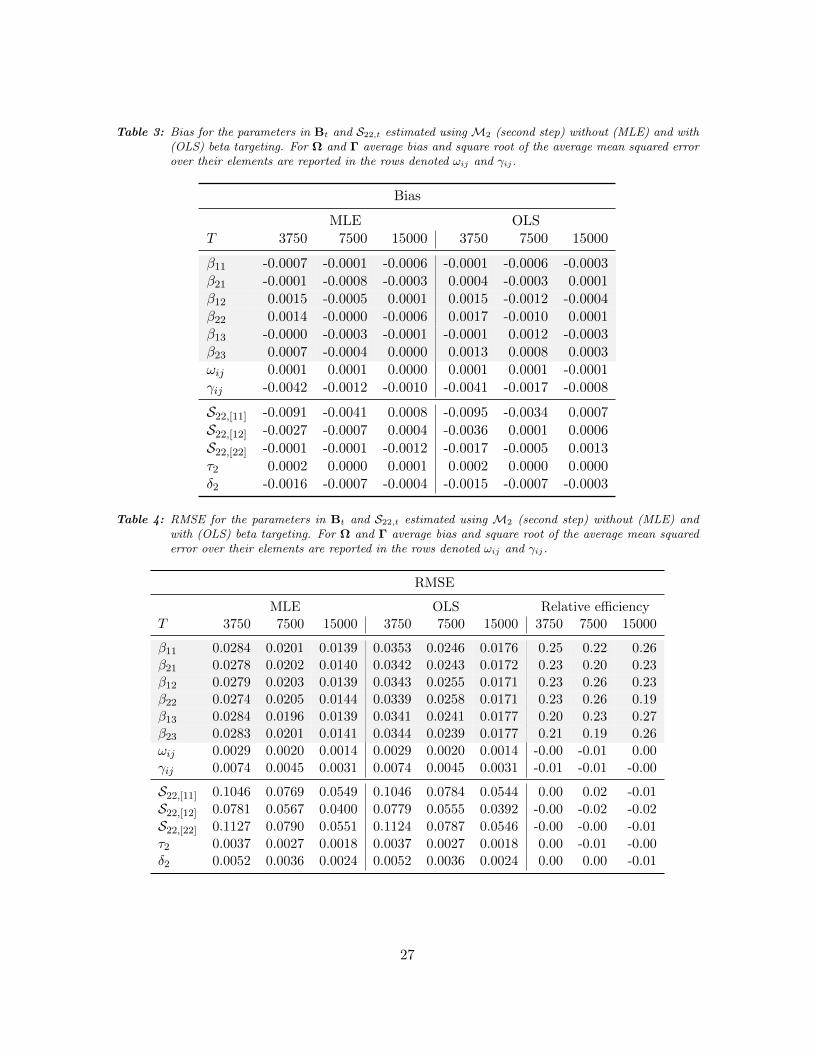
Table 3: Bias for the parameters in Bt and S22,t estimated using M2 (second step) without (MLE) and with(OLS) beta targeting. For Ω and Γ average bias and square root of the average mean squared errorover their elements are reported in the rows denoted ωij and γij.

Bias

MLE OLST 3750 7500 15000 3750 7500 15000

β11 -0.0007 -0.0001 -0.0006 -0.0001 -0.0006 -0.0003β21 -0.0001 -0.0008 -0.0003 0.0004 -0.0003 0.0001β12 0.0015 -0.0005 0.0001 0.0015 -0.0012 -0.0004β22 0.0014 -0.0000 -0.0006 0.0017 -0.0010 0.0001β13 -0.0000 -0.0003 -0.0001 -0.0001 0.0012 -0.0003β23 0.0007 -0.0004 0.0000 0.0013 0.0008 0.0003ωij 0.0001 0.0001 0.0000 0.0001 0.0001 -0.0001γij -0.0042 -0.0012 -0.0010 -0.0041 -0.0017 -0.0008

S22,[11] -0.0091 -0.0041 0.0008 -0.0095 -0.0034 0.0007

S22,[12] -0.0027 -0.0007 0.0004 -0.0036 0.0001 0.0006

S22,[22] -0.0001 -0.0001 -0.0012 -0.0017 -0.0005 0.0013

τ2 0.0002 0.0000 0.0001 0.0002 0.0000 0.0000δ2 -0.0016 -0.0007 -0.0004 -0.0015 -0.0007 -0.0003

Table 4: RMSE for the parameters in Bt and S22,t estimated using M2 (second step) without (MLE) andwith (OLS) beta targeting. For Ω and Γ average bias and square root of the average mean squarederror over their elements are reported in the rows denoted ωij and γij.

RMSE

MLE OLS Relative efficiencyT 3750 7500 15000 3750 7500 15000 3750 7500 15000

β11 0.0284 0.0201 0.0139 0.0353 0.0246 0.0176 0.25 0.22 0.26β21 0.0278 0.0202 0.0140 0.0342 0.0243 0.0172 0.23 0.20 0.23β12 0.0279 0.0203 0.0139 0.0343 0.0255 0.0171 0.23 0.26 0.23β22 0.0274 0.0205 0.0144 0.0339 0.0258 0.0171 0.23 0.26 0.19β13 0.0284 0.0196 0.0139 0.0341 0.0241 0.0177 0.20 0.23 0.27β23 0.0283 0.0201 0.0141 0.0344 0.0239 0.0177 0.21 0.19 0.26ωij 0.0029 0.0020 0.0014 0.0029 0.0020 0.0014 -0.00 -0.01 0.00γij 0.0074 0.0045 0.0031 0.0074 0.0045 0.0031 -0.01 -0.01 -0.00

S22,[11] 0.1046 0.0769 0.0549 0.1046 0.0784 0.0544 0.00 0.02 -0.01

S22,[12] 0.0781 0.0567 0.0400 0.0779 0.0555 0.0392 -0.00 -0.02 -0.02

S22,[22] 0.1127 0.0790 0.0551 0.1124 0.0787 0.0546 -0.00 -0.00 -0.01

τ2 0.0037 0.0027 0.0018 0.0037 0.0027 0.0018 0.00 -0.01 -0.00δ2 0.0052 0.0036 0.0024 0.0052 0.0036 0.0024 0.00 0.00 -0.01

27

(P ). The three risk factors are: the market factor (fmkt,t), given by the excess return of the

value-weight portfolio formed by all US firms listed on the NYSE, AMEX, or NASDAQ; the size

factor (small-minus-big, fsmb,t) given by a long-short self-financing portfolio of value weighted

returns sorted by size; and the value factor (high-minus-low, fhml,t) given by a long-short self-

financing portfolio of value-weighted returns sorted by book-to-market ratio. The sample spans

the period from January 1, 1927 to October, 30 2020, totaling 24682 daily observations. The data

is obtained from Kenneth French’s website data library.23 The three factors and the two industry

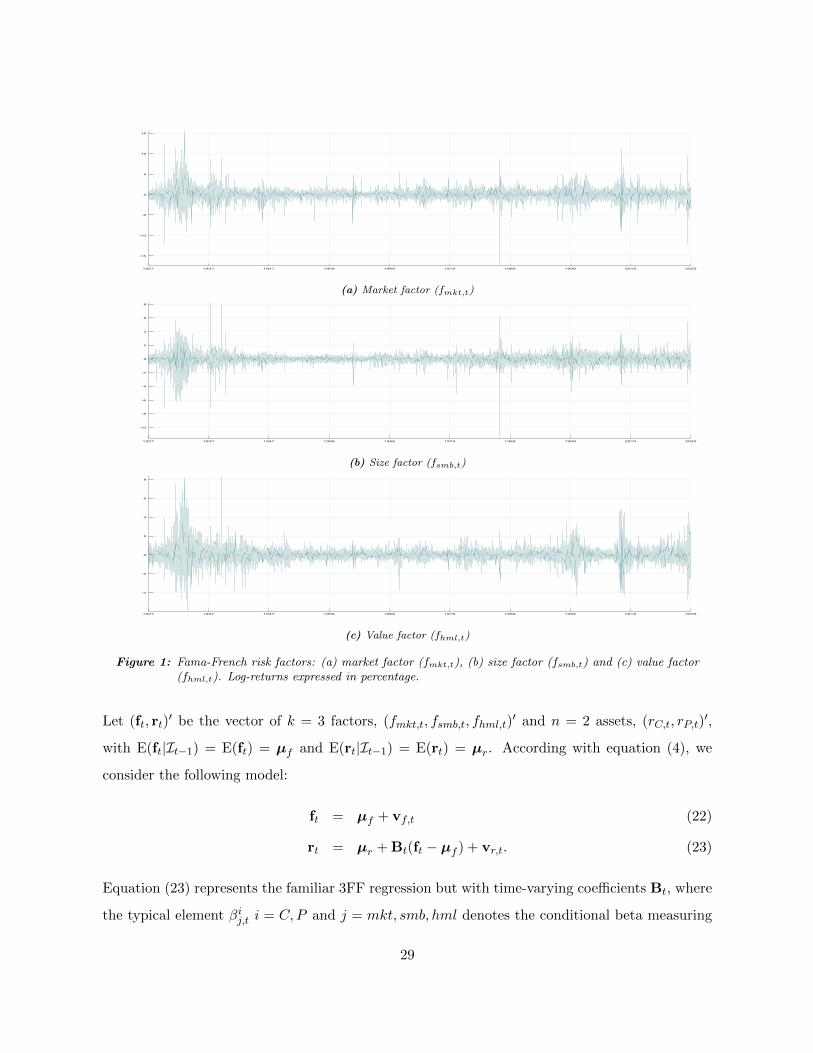
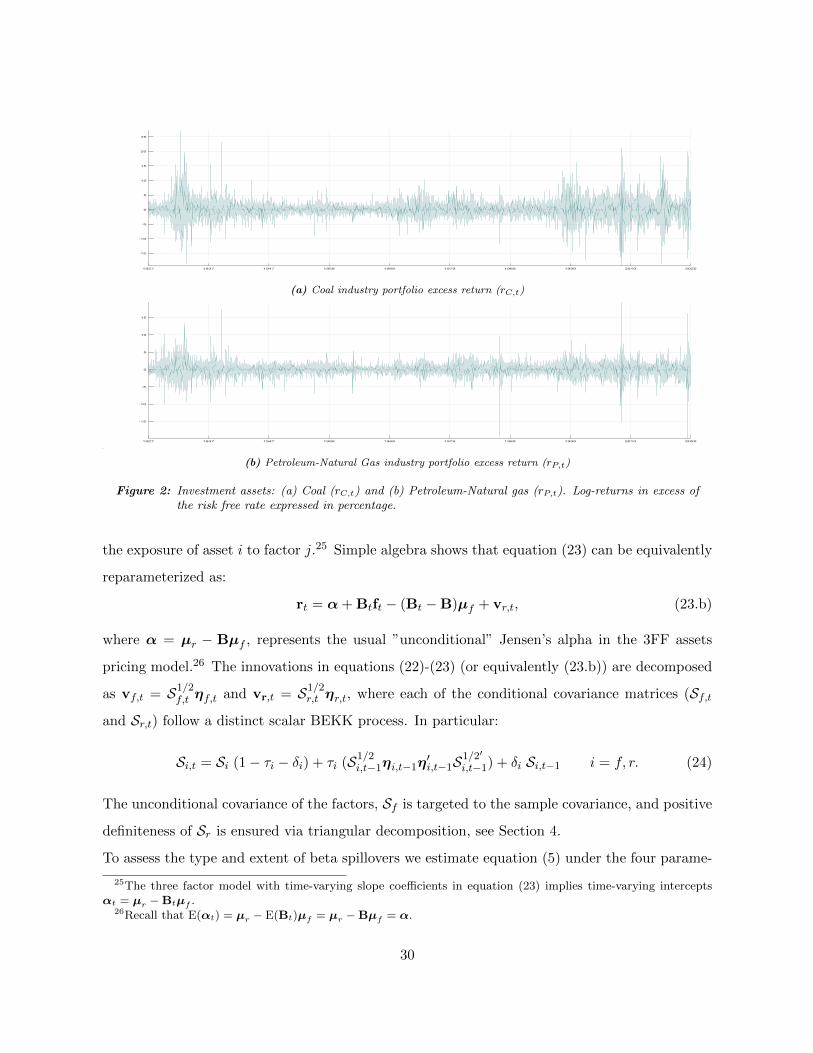
portfolios log-returns in excess of the risk-free rate are plotted in Figures 1 and 2, respectively.

In the figures are visible the long lasting volatility cluster of the Great depression (1929-1939),

the effects of the oil shocks in the 70s, the drop of the Black Monday in October 1987, the turmoil

of late 90s-early 2000s (1997 Asian financial crisis, 1998 Russian financial crisis, 2000 dot-com

bubble burst, 2001 9/11 events, 2002 US stock market downturn), the 2007-8 global financial

crisis followed by the European sovereign debt crisis, and, last, the 2020 COVID-19 pandemic.

In Figure 2, it is also visible the 2015-16 Chinese stock market crash, which set off a global stock

market sell-off and a steep drop in commodities prices.

The second application uses the BC-GARCH to estimate the risk premia attached to risk factors

exposures. We test the linear conditional beta pricing model used in Fama and MacBeth (1973)

in the CAPM and 3FF frameworks. We benchmark the BC-GARCH against the 2PR approach

of Fama and MacBeth (1973). The cross-section of assets consists of returns on 40 value-weighed

industry portfolios.24 For sake of comparability with the existing literature, we use a monthly

aggregation frequency, totaling 1126 observations.

5.1 Beta Spillovers in the Coal and Petroleum-Natural Gas industry portfolios

The two-blocks partition of equation (4) lends itself to the linear asset pricing context, naturally

fitting the distinction between market-wide risk factors and investment assets.

23The composition of the two industry portfolios based on their four-digit SIC code is available athttp://mba.tuck.dartmouth.edu/pages/faculty/ken.french/ftp/Siccodes30.zip. The two portfolios are number 18and 19 respectively of the list of 30 industry portfolios. The dataset containing daily returns on the industry portfo-lios and the the factors is available at http://mba.tuck.dartmouth.edu/pages/ faculty/ken.french/data library.html

24The data used is a subset extracted from the collection of 48 industry portfolios available at Kenneth French’sdata library. We exclude 8 portfolios, 3, 11, 15, 20, 26, 27, 33, 38, for which returns are available only over ashorter time span.

28

1927 1937 1947 1958 1968 1979 1989 1999 2010 2020

-15

-10

-5

0

5

10

15

(a) Market factor (fmkt,t)

1927 1937 1947 1958 1968 1979 1989 1999 2010 2020

-10

-8

-6

-4

-2

0

2

4

6

8

(b) Size factor (fsmb,t)

1927 1937 1947 1958 1968 1979 1989 1999 2010 2020

-4

-2

0

2

4

6

8

(c) Value factor (fhml,t)

Figure 1: Fama-French risk factors: (a) market factor (fmkt,t), (b) size factor (fsmb,t) and (c) value factor(fhml,t). Log-returns expressed in percentage.

Let (ft, rt)′ be the vector of k = 3 factors, (fmkt,t, fsmb,t, fhml,t)

′ and n = 2 assets, (rC,t, rP,t)′,

with E(ft|It−1) = E(ft) = µf and E(rt|It−1) = E(rt) = µr. According with equation (4), we

consider the following model:

ft = µf + vf,t (22)

rt = µr + Bt(ft − µf ) + vr,t. (23)

Equation (23) represents the familiar 3FF regression but with time-varying coefficients Bt, where

the typical element βij,t i = C,P and j = mkt, smb, hml denotes the conditional beta measuring

29

1927 1937 1947 1958 1968 1979 1989 1999 2010 2020

-15

-10

-5

0

5

10

15

20

25

(a) Coal industry portfolio excess return (rC,t)

1927 1937 1947 1958 1968 1979 1989 1999 2010 2020

-15

-10

-5

0

5

10

15

(b) Petroleum-Natural Gas industry portfolio excess return (rP,t)

Figure 2: Investment assets: (a) Coal (rC,t) and (b) Petroleum-Natural gas (rP,t). Log-returns in excess ofthe risk free rate expressed in percentage.

the exposure of asset i to factor j.25 Simple algebra shows that equation (23) can be equivalently

reparameterized as:

rt = α+ Btft − (Bt −B)µf + vr,t, (23.b)

where α = µr − Bµf , represents the usual ”unconditional” Jensen’s alpha in the 3FF assets

pricing model.26 The innovations in equations (22)-(23) (or equivalently (23.b)) are decomposed

as vf,t = S1/2f,t ηf,t and vr,t = S1/2

r,t ηr,t, where each of the conditional covariance matrices (Sf,tand Sr,t) follow a distinct scalar BEKK process. In particular:

Si,t = Si (1− τi − δi) + τi (S1/2i,t−1ηi,t−1η

′i,t−1S

1/2′

i,t−1) + δi Si,t−1 i = f, r. (24)

The unconditional covariance of the factors, Sf is targeted to the sample covariance, and positive

definiteness of Sr is ensured via triangular decomposition, see Section 4.

To assess the type and extent of beta spillovers we estimate equation (5) under the four parame-

25The three factor model with time-varying slope coefficients in equation (23) implies time-varying interceptsαt = µr −Btµf .

26Recall that E(αt) = µr − E(Bt)µf = µr −Bµf = α.

30

ter restrictions: i) idiosyncratic shocks, which constitutes the benchmark specification, ii) factor

spillovers, iii) asset spillovers and, iv) both asset and factor spillovers. To contain the number of

parameters and thus reduce the computational burden, we allow spillovers of shocks via the matrix

Ω (direct effect), while we restrict the contribution of the smoothing term (feedback) to be idiosyn-

cratic. This is achieved by constraining the matrix of parameters Γ to be diagonal. For the sake

of feasibility, we also target the unconditional level of Bt to the OLS estimate. This is done via

reparameterization of the intercept in equation (5) as Ψ = BOLS(

vec−1(k×n)

(diag(I(nk) − Γ)

))′.

Finally, to avoid the aforementioned problem of reduction in the scale of the innovations driving

the dynamics of the conditional beta induced by the block orthogonalization, as well as to reduce

the impact of abnormally large shocks, we let Bt depend on products of devolatilized innovations.

The model’s parameter are estimated by QML using the two-step approach, M2.

Table 5 reports the second step estimation results for the four conditional beta specifications

and the covariance equation. Note that the inference on the elements of the unconditional

beta matrix B are based on OLS. For the other parameters, QML standard errors are com-

puted using the sandwich formula.27 For the Coal industry portfolio, the unconditional expo-

sure to the market factor amounts to 1.17 denoting a portfolio fairly correlated with the market,

(Corr(rC,t, fmkt,t) = 0.59) but sensibly more volatile (Var(rC,t) = 4.64 against Var(fmkt,t) = 1.17).

This portfolio appears to be also unconditionally exposed to the size factor (βCsmb = 0.45), as well

as the value factor (βChml = 0.51). Turning to the Petroleum-Natural Gas industry portfolio, the

unconditional beta associated to the market factor is slightly below one. This portfolio, despite

being more correlated with the market (Corr(rP,t, fmkt,t) = 0.78), exhibits a much less erratic be-

havior (Var(rP,t) = 1.76). Unconditional exposure to the size factor is negative but close to zero.

Finally, with respect to the unconditional exposure to the value factor the Petroleum-Natural

Gas industry portfolio shows levels comparable to what observed for the Coal industry portfolio

(βPhml = 0.54).

For all six conditional betas we find evidence of time variation characterized by highly persistent

dynamics. The estimated smoothing coefficients are very close to one, with the γi,j coefficients

ranging from 0.9966 to 0.9996. These results are in line with the findings of Darolles, Francq,

27Parameter estimates (standard errors) for the first step are τf = 0.0641 (0.0031) and δf = 0.9327 (0.0033).

31

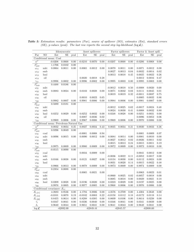
Table 5: Estimation results: parameters (Par), source of spillover (SO), estimates (Est), standard errors(SE), p-values (pval). The last row reports the second step log-likelihood (logL).

Idiosyncratic Asset spillovers Factor spillovers Factor & Asset spill.

Par SO Est SE pval Est SE pval Est SE pval Est SE pval

Conditional mean: Coal

αC -0.0208 0.0068 0.00 -0.0210 0.0070 0.00 -0.0207 0.0068 0.00 -0.0206 0.0068 0.00

βCmkt 1.1706 0.0102 0.00ω11 mkt 0.0064 0.0011 0.00 0.0065 0.0012 0.00 0.0070 0.0011 0.00 0.0071 0.0012 0.00ω12 smb 0.0027 0.0013 0.04 0.0032 0.0014 0.02ω13 hml 0.0013 0.0018 0.45 0.0025 0.0022 0.26ω14 oil 0.0020 0.0018 0.28 0.0012 0.0016 0.47γ11 0.9996 0.0002 0.00 0.9996 0.0002 0.00 0.9995 0.0003 0.00 0.9995 0.0003 0.00

βCsmb 0.4488 0.0186 0.00ω21 mkt -0.0012 0.0018 0.50 -0.0008 0.0020 0.68ω22 smb 0.0083 0.0024 0.00 0.0103 0.0028 0.00 0.0071 0.0032 0.03 0.0111 0.0045 0.01ω23 hml 0.0019 0.0019 0.32 -0.0011 0.0037 0.75ω25 oil 0.0010 0.0023 0.65 0.0005 0.0032 0.86γ22 0.9982 0.0007 0.00 0.9981 0.0006 0.00 0.9984 0.0006 0.00 0.9981 0.0007 0.00

βChml 0.5089 0.0181 0.00ω31 mkt -0.0012 0.0025 0.62 -0.0017 0.0024 0.48ω32 smb 0.0024 0.0030 0.41 0.0008 0.0032 0.80ω33 hml 0.0252 0.0029 0.00 0.0252 0.0032 0.00 0.0248 0.0028 0.00 0.0251 0.0031 0.00ω36 oil 0.0087 0.0036 0.02 0.0096 0.0052 0.06γ33 0.9969 0.0006 0.00 0.9967 0.0006 0.00 0.9969 0.0006 0.00 0.9970 0.0006 0.00

Conditional mean: Petroleum-Natural Gas

αP 0.0032 0.0034 0.35 0.0027 0.0034 0.43 0.0035 0.0034 0.31 0.0030 0.0033 0.36

βPmkt 0.9296 0.0049 0.00ω41 coal -0.0001 0.0008 0.94 0.0001 0.0009 0.97ω44 mkt 0.0096 0.0015 0.00 0.0090 0.0012 0.00 0.0084 0.0014 0.00 0.0081 0.0010 0.00ω45 smb -0.0027 0.0012 0.02 -0.0026 0.0011 0.02ω46 hml 0.0015 0.0013 0.24 0.0015 0.0011 0.19γ44 0.9975 0.0009 0.00 0.9980 0.0009 0.00 0.9972 0.0009 0.00 0.9973 0.0010 0.00

βPsmb -0.0515 0.0090 0.00ω52 coal 0.0034 0.0009 0.00 0.0041 0.0012 0.00ω54 mkt -0.0036 0.0022 0.11 -0.0052 0.0017 0.00ω55 smb 0.0166 0.0038 0.00 0.0121 0.0027 0.00 0.0134 0.0030 0.00 0.0112 0.0024 0.00ω56 hml 0.0031 0.0020 0.14 0.0015 0.0022 0.48γ55 0.9966 0.0013 0.00 0.9978 0.0009 0.00 0.9973 0.0009 0.00 0.9974 0.0009 0.00

βPhml 0.2354 0.0088 0.00ω63 coal 0.0065 0.0021 0.00 0.0063 0.0023 0.01ω64 mkt -0.0060 0.0025 0.02 -0.0057 0.0018 0.00ω65 smb 0.0085 0.0018 0.00 0.0029 0.0021 0.18ω66 hml 0.0209 0.0028 0.00 0.0196 0.0020 0.00 0.0223 0.0029 0.00 0.0197 0.0025 0.00γ66 0.9976 0.0005 0.00 0.9977 0.0005 0.00 0.9968 0.0006 0.00 0.9976 0.0006 0.00

Conditional covariance: Sr,tSr,[11] 4.2683 0.9536 0.00 4.1794 0.8806 0.00 4.3576 0.2709 0.00 4.4304 0.2648 0.00

Sr,[12] -0.0101 0.0078 0.19 -0.0102 0.0083 0.22 -0.0150 0.0112 0.18 -0.0172 0.0118 0.14

Sr,[22] 0.8455 0.0614 0.00 0.8208 0.0385 0.00 0.8609 0.0106 0.00 0.8614 0.0238 0.00

τr 0.0347 0.0041 0.00 0.0336 0.0040 0.00 0.0346 0.0041 0.00 0.0341 0.0039 0.00δr 0.9640 0.0044 0.00 0.9651 0.0041 0.00 0.9641 0.0043 0.00 0.9648 0.0041 0.00

logL -62892.00 -62849.44 -62845.57 -62808.60

32

and Laurent (2018) for a comparable modeling approach and the same sampling frequency and

assets class.

We also find evidence of both factor and asset spillovers. More precisely, with respect to factor

spillovers, we find that shocks in the size factor (fsmb,t), impact the exposure of both portfolios

to the market factor, albeit in opposite direction for βCmkt,t and βPmkt,t. Evidence specific to each

portfolio is found when looking at the exposure to the size and the value factors. For the Coal

industry portfolio, we do not find any evidence of spillovers on βCsmb,t, while we find statisti-

cally significant asset spillovers on βChml. For the Petroleum-Natural Gas industry portfolio, the

spillovers in the exposures to fsmb,t and fhml,t involve to both asset and factor spillovers. The

source of the spillover is, in both cases, limited to the market factor.

It is worth recalling that equation (5) under the restrictions in iv) nests the parameterizations

in i), ii) and iii). Estimates of the parameters associated to the idiosyncratic shock, common to

all specifications, are found to be close across specifications. This suggests that the inclusion of

spillovers, although not independent nor orthogonal to the idiosyncratic shock, provide novel and

relevant information. This is confirmed by the likelihood ratio test which finds the specification

allowing for both assets and factors spillovers statistically superior to the others at standard

confidence levels. We rely on this specification for all results in the reminder of this section.

Finally, the 3FF model predicts that the risk factors are sufficient to price assets. Formally,

the intercept in equation (23.b) (α = (αC , αP )′), is expected to vanish. When testing the null

hypothesis αn = 0, n = C,P individually, the intercept, αP , is not statistically different from

zero. The zero intercept hypothesis, is instead rejected for the Coal industry portfolio, suggesting

possible misspecification of the pricing model.

Figures 3 and 4 report the six filtered conditional betas, βnj,t, n = C,P and j = mkt, smb, hml for

the specification in equation (5) in the parameterisation iv). Each plot contains the conditional

beta estimated by the BC-GARCH (black), as well as those obtained using two competing ap-

proaches: the indirect estimation of the DCB-DCC model (green) and the rolling OLS estimator

with a window of 100 observations (red). The horizontal line represents the unconditional beta

estimated by full-sample OLS.

Note that for the rolling OLS estimator, smoother sample paths are to be expected for larger

33

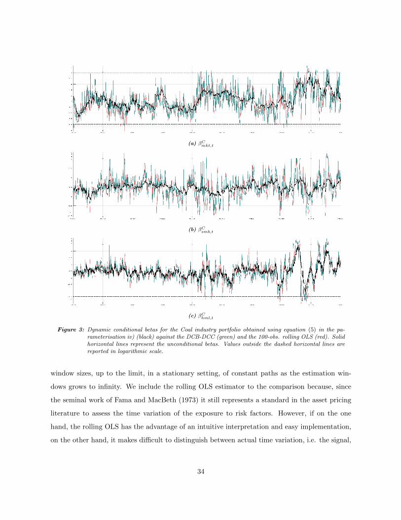
(a) βCmkt,t

(b) βCsmb,t

(c) βChml,t

Figure 3: Dynamic conditional betas for the Coal industry portfolio obtained using equation (5) in the pa-rameterisation iv) (black) against the DCB-DCC (green) and the 100-obs. rolling OLS (red). Solidhorizontal lines represent the unconditional betas. Values outside the dashed horizontal lines arereported in logarithmic scale.

window sizes, up to the limit, in a stationary setting, of constant paths as the estimation win-

dows grows to infinity. We include the rolling OLS estimator to the comparison because, since

the seminal work of Fama and MacBeth (1973) it still represents a standard in the asset pricing

literature to assess the time variation of the exposure to risk factors. However, if on the one

hand, the rolling OLS has the advantage of an intuitive interpretation and easy implementation,

on the other hand, it makes difficult to distinguish between actual time variation, i.e. the signal,

34

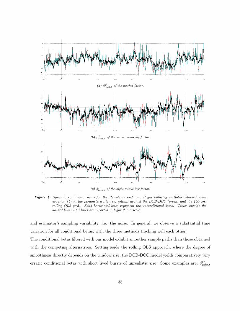
(a) βPmkt,t of the market factor.

(b) βPsmb,t of the small minus big factor.

(c) βPhml,t of the hight-minus-low factor.

Figure 4: Dynamic conditional betas for the Petroleum and natural gas industry portfolio obtained usingequation (5) in the parameterisation iv) (black) against the DCB-DCC (green) and the 100-obs.rolling OLS (red). Solid horizontal lines represent the unconditional betas. Values outside thedashed horizontal lines are reported in logarithmic scale.

and estimator’s sampling variability, i.e. the noise. In general, we observe a substantial time

variation for all conditional betas, with the three methods tracking well each other.

The conditional betas filtered with our model exhibit smoother sample paths than those obtained

with the competing alternatives. Setting aside the rolling OLS approach, where the degree of

smoothness directly depends on the window size, the DCB-DCC model yields comparatively very

erratic conditional betas with short lived bursts of unrealistic size. Some examples are, βCmkt,t

35

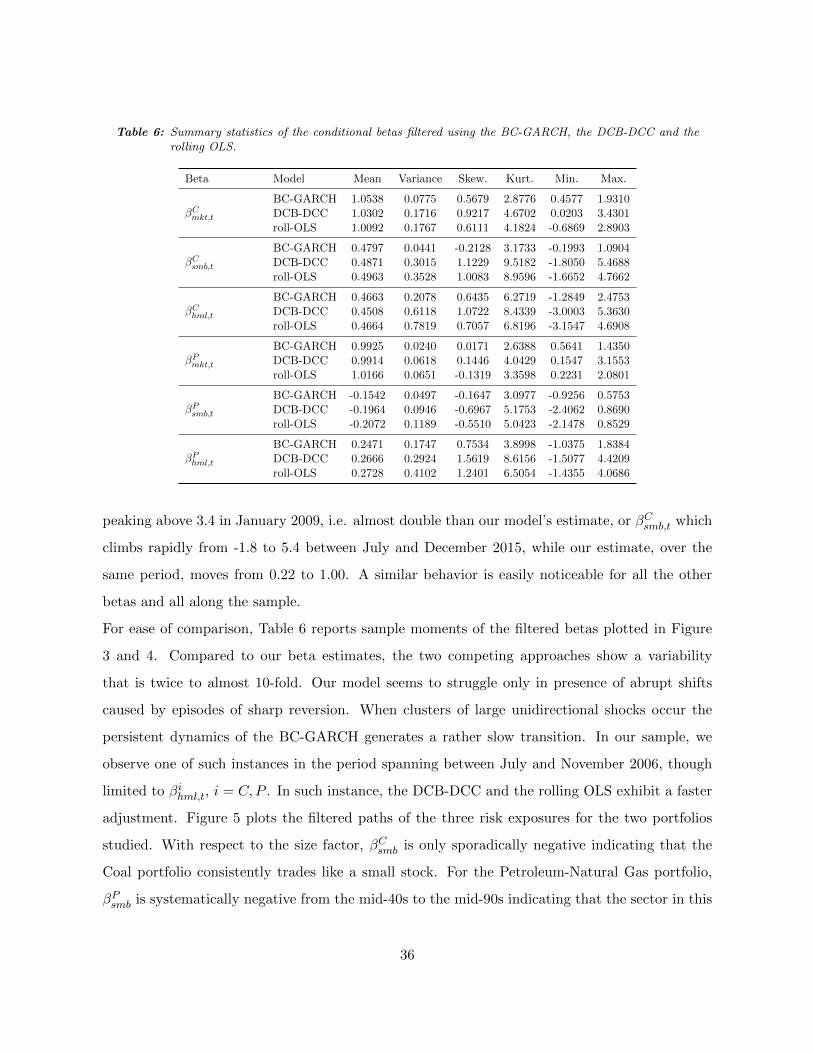
Table 6: Summary statistics of the conditional betas filtered using the BC-GARCH, the DCB-DCC and therolling OLS.

Beta Model Mean Variance Skew. Kurt. Min. Max.

βCmkt,t

BC-GARCH 1.0538 0.0775 0.5679 2.8776 0.4577 1.9310DCB-DCC 1.0302 0.1716 0.9217 4.6702 0.0203 3.4301roll-OLS 1.0092 0.1767 0.6111 4.1824 -0.6869 2.8903

βCsmb,t

BC-GARCH 0.4797 0.0441 -0.2128 3.1733 -0.1993 1.0904DCB-DCC 0.4871 0.3015 1.1229 9.5182 -1.8050 5.4688roll-OLS 0.4963 0.3528 1.0083 8.9596 -1.6652 4.7662

βChml,t

BC-GARCH 0.4663 0.2078 0.6435 6.2719 -1.2849 2.4753DCB-DCC 0.4508 0.6118 1.0722 8.4339 -3.0003 5.3630roll-OLS 0.4664 0.7819 0.7057 6.8196 -3.1547 4.6908

βPmkt,t

BC-GARCH 0.9925 0.0240 0.0171 2.6388 0.5641 1.4350DCB-DCC 0.9914 0.0618 0.1446 4.0429 0.1547 3.1553roll-OLS 1.0166 0.0651 -0.1319 3.3598 0.2231 2.0801

βPsmb,t

BC-GARCH -0.1542 0.0497 -0.1647 3.0977 -0.9256 0.5753DCB-DCC -0.1964 0.0946 -0.6967 5.1753 -2.4062 0.8690roll-OLS -0.2072 0.1189 -0.5510 5.0423 -2.1478 0.8529

βPhml,t

BC-GARCH 0.2471 0.1747 0.7534 3.8998 -1.0375 1.8384DCB-DCC 0.2666 0.2924 1.5619 8.6156 -1.5077 4.4209roll-OLS 0.2728 0.4102 1.2401 6.5054 -1.4355 4.0686

peaking above 3.4 in January 2009, i.e. almost double than our model’s estimate, or βCsmb,t which

climbs rapidly from -1.8 to 5.4 between July and December 2015, while our estimate, over the

same period, moves from 0.22 to 1.00. A similar behavior is easily noticeable for all the other

betas and all along the sample.

For ease of comparison, Table 6 reports sample moments of the filtered betas plotted in Figure

3 and 4. Compared to our beta estimates, the two competing approaches show a variability

that is twice to almost 10-fold. Our model seems to struggle only in presence of abrupt shifts

caused by episodes of sharp reversion. When clusters of large unidirectional shocks occur the

persistent dynamics of the BC-GARCH generates a rather slow transition. In our sample, we

observe one of such instances in the period spanning between July and November 2006, though

limited to βihml,t, i = C,P . In such instance, the DCB-DCC and the rolling OLS exhibit a faster

adjustment. Figure 5 plots the filtered paths of the three risk exposures for the two portfolios

studied. With respect to the size factor, βCsmb is only sporadically negative indicating that the

Coal portfolio consistently trades like a small stock. For the Petroleum-Natural Gas portfolio,

βPsmb is systematically negative from the mid-40s to the mid-90s indicating that the sector in this

36

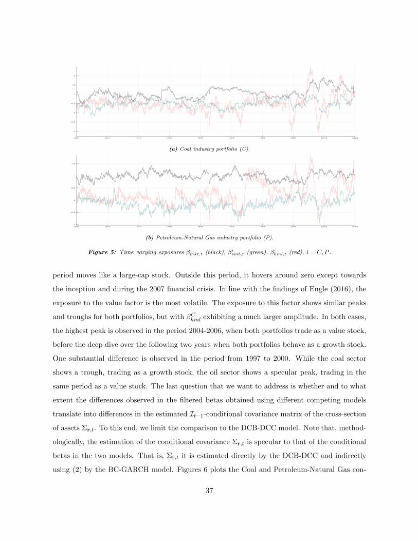
1927 1937 1947 1958 1968 1979 1989 1999 2010 2020

-1

-0.5

0

0.5

1

1.5

2

(a) Coal industry portfolio (C).

1927 1937 1947 1958 1968 1979 1989 1999 2010 2020

-1

-0.5

0

0.5

1

1.5

(b) Petroleum-Natural Gas industry portfolio (P).

Figure 5: Time varying exposures βimkt,t (black), βi

smb,t (green), βihml,t (red), i = C,P .

period moves like a large-cap stock. Outside this period, it hovers around zero except towards

the inception and during the 2007 financial crisis. In line with the findings of Engle (2016), the

exposure to the value factor is the most volatile. The exposure to this factor shows similar peaks

and troughs for both portfolios, but with βChml exhibiting a much larger amplitude. In both cases,

the highest peak is observed in the period 2004-2006, when both portfolios trade as a value stock,

before the deep dive over the following two years when both portfolios behave as a growth stock.

One substantial difference is observed in the period from 1997 to 2000. While the coal sector

shows a trough, trading as a growth stock, the oil sector shows a specular peak, trading in the

same period as a value stock. The last question that we want to address is whether and to what

extent the differences observed in the filtered betas obtained using different competing models

translate into differences in the estimated It−1-conditional covariance matrix of the cross-section

of assets Σr,t. To this end, we limit the comparison to the DCB-DCC model. Note that, method-

ologically, the estimation of the conditional covariance Σr,t is specular to that of the conditional

betas in the two models. That is, Σr,t it is estimated directly by the DCB-DCC and indirectly

using (2) by the BC-GARCH model. Figures 6 plots the Coal and Petroleum-Natural Gas con-

37

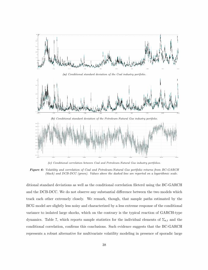
(a) Conditional standard deviation of the Coal industry portfolio.

(b) Conditional standard deviation of the Petroleum-Natural Gas industry portfolio.

1927 1937 1947 1958 1968 1979 1989 1999 2010 2020

-0.1

0

0.1

0.2

0.3

0.4

0.5

0.6

0.7

0.8

0.9

(c) Conditional correlation between Coal and Petroleum-Natural Gas industry portfolios.

Figure 6: Volatility and correlation of Coal and Petroleum-Natural Gas portfolio returns from BC-GARCH(black) and DCB-DCC (green). Values above the dashed line are reported on a logarithmic scale.

ditional standard deviations as well as the conditional correlation fileterd using the BC-GARCH

and the DCB-DCC. We do not observe any substantial difference between the two models which

track each other extremely closely. We remark, though, that sample paths estimated by the

BCG model are slightly less noisy and characterized by a less extreme response of the conditional

variance to isolated large shocks, which on the contrary is the typical reaction of GARCH-type

dynamics. Table 7, which reports sample statistics for the individual elements of Σr,t and the

conditional correlation, confirms this conclusions. Such evidence suggests that the BC-GARCH

represents a robust alternative for multivariate volatility modeling in presence of sporadic large

38

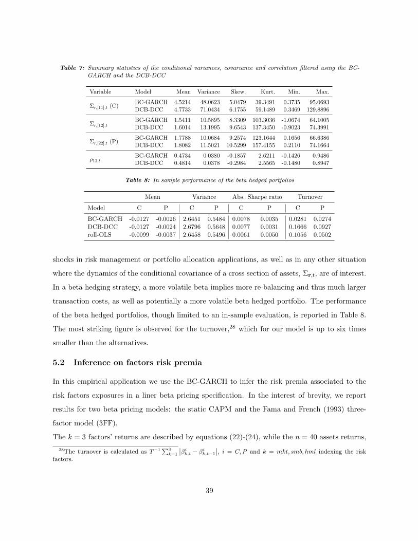
Table 7: Summary statistics of the conditional variances, covariance and correlation filtered using the BC-GARCH and the DCB-DCC

Variable Model Mean Variance Skew. Kurt. Min. Max.

Σr,[11],t (C)BC-GARCH 4.5214 48.0623 5.0479 39.3491 0.3735 95.0693DCB-DCC 4.7733 71.0434 6.1755 59.1489 0.3469 129.8896

Σr,[12],tBC-GARCH 1.5411 10.5895 8.3309 103.3036 -1.0674 64.1005DCB-DCC 1.6014 13.1995 9.6543 137.3450 -0.9023 74.3991

Σr,[22],t (P)BC-GARCH 1.7788 10.0684 9.2574 123.1644 0.1656 66.6386DCB-DCC 1.8082 11.5021 10.5299 157.4155 0.2110 74.1664

ρ12,tBC-GARCH 0.4734 0.0380 -0.1857 2.6211 -0.1426 0.9486DCB-DCC 0.4814 0.0378 -0.2984 2.5565 -0.1480 0.8947

Table 8: In sample performance of the beta hedged portfolios

Mean Variance Abs. Sharpe ratio Turnover

Model C P C P C P C P

BC-GARCH -0.0127 -0.0026 2.6451 0.5484 0.0078 0.0035 0.0281 0.0274DCB-DCC -0.0127 -0.0024 2.6796 0.5648 0.0077 0.0031 0.1666 0.0927roll-OLS -0.0099 -0.0037 2.6458 0.5496 0.0061 0.0050 0.1056 0.0502

shocks in risk management or portfolio allocation applications, as well as in any other situation

where the dynamics of the conditional covariance of a cross section of assets, Σr,t, are of interest.

In a beta hedging strategy, a more volatile beta implies more re-balancing and thus much larger

transaction costs, as well as potentially a more volatile beta hedged portfolio. The performance

of the beta hedged portfolios, though limited to an in-sample evaluation, is reported in Table 8.

The most striking figure is observed for the turnover,28 which for our model is up to six times

smaller than the alternatives.

5.2 Inference on factors risk premia

In this empirical application we use the BC-GARCH to infer the risk premia associated to the

risk factors exposures in a liner beta pricing specification. In the interest of brevity, we report

results for two beta pricing models: the static CAPM and the Fama and French (1993) three-

factor model (3FF).

The k = 3 factors’ returns are described by equations (22)-(24), while the n = 40 assets returns,

28The turnover is calculated as T−1∑3k=1

∣∣βik,t − βi

k,t−1

∣∣, i = C,P and k = mkt, smb, hml indexing the riskfactors.

39

conditional to the risk factors, are described by:

rt = µr,t + Bt(ft − µf ) + vr,t, (25)

with µr,t = E(rt|It−1) and vr,t = S1/2r,t ηr,t. Assuming µr,t = µr, equation (25) boils down to

equation (23). In this case the null hypothesis H0 : µr,t = Bµf or equivalently H0 : αi = 0,

i = 1, . . . , n, in equation (23.b), represents a simple misspecification test for the pricing model.

The test can be carried out individually or jointly, by exploiting the multivariate representation

in equation (23.b).29 Despite its usefulness, equation (23.b) cannot identify the source and the

form of the risk-return trade-off.

Following Connor (1984), a more appealing testable hypothesis expresses the conditional expec-

tation of the assets return as:

E(rt|It−1) = δ + Btλ, (26)

that is a linear conditional beta pricing specification, where λ = λ1, . . . , λk, is the vector of

risk premia attached to the factor exposure. Note that δ and λ are invariant in the cross-section.

Our joint specification in equation (25) can easily integrate this restriction.30

The linear conditional pricing specification in equation (26) measures explicitly the size of the

risk-return trade-off and represents a misspecification test of the pricing model, see Sharpe (1964)

and Lintner (1965). For example, in the CAPM framework, assuming market and assets returns

are both expressed in excess of the risk free rate, misspecification of the pricing model takes the

form of the Sharpe-Lintner hypothesis H0 : δ = 0 ∩ λ = µmkt.31

To explicitly account for misspecification of the asset return in the form of omitted priced factors,

Kleibergen (2009) relaxes equation (26) by introducing a fixed idiosyncratic effect of the form:

E(rt|It−1) = δ0 + δ + Btλ. (27)

Under the suitable identification restriction δi = 0, for some i ∈ [1, n]. The idiosyncratic intercepts

make it possible to test the restriction δ = 0, rather than imposing it a priori. It also preserves the

validity of the QML inference when the restriction is violated, by ensuring that the innovations

29Note that this is the standing hypothesis in a constant beta framework.30Other specifications such as quadratic beta pricing, beta interactions or systematic effects of non-β risks could

also be evaluated, see Fama and MacBeth (1973) for a variety of specifications.31Such hypothesis is, in fact, equivalent to H0 : α = 0 in equation (23.b).

40

are centered over the time dimension. Thus, in a multi-factor asset pricing specification, the

linear conditional pricing model can be expressed as:

ft = µf + vf,t, (28)

rt = δ0 + δ + Bt (ft − µf + λ) + vr,t. (29)

A large cross-sectional dimension, as the one considered in our application, inevitably translates

in a substantial number of parameters which in turn may hinder the computational feasibility.

To attenuate the curse of dimensionality we impose the following restrictions. First, since our

interest is on the risk premia λ, we remove the individual effect by centering the returns around

their unconditional expectation. Equation (29) is reparameterized as:

rt − µr = (Bt −B)λ+ Bt (ft − µf ) + vr,t. (30)

Second, we adopt a simple and parsimonious dynamics for the matrix of conditional betas Bt by

imposing cross-sectional restrictions. To this end, we assume Bt follows the semi-scalar dynamics

described in Section 3.4. Together with beta tracking, i.e. B is targeted to the OLS estimator,

the conditional beta specification takes the form:

Bt = B[e(n) ×

(e′(k) − γ

′(k)

) ]+ e(n)ω

′(k)

(ξr,tξ

′f,t

)+ e(n)γ

′(k) Bt−1. (31)

Third, similar considerations hold for the dynamics of the conditional covariance matrix Sr,t.

Because covariance targeting is unfeasible for Sr,t and since only its diagonal elements are required

to standardize the innovations in equation (31), we rely on the marginalization of the scalar

BEKK model. This allows us to reduce the number of parameters by n(n − 1)/2, which in this

case amounts to 780 nuisance unconditional covariances.

Fourth, compatibly with the choices described above, i.e. cross-sectional constraints together

with marginalization, we estimate the model’s parameters usingM4 detailed in Section 3.6. The

total number of parameters estimated by Gaussian QML, via log-transformation of equation (17)

and (18), is 53.32

We benchmark our model against the 2-Pass Cross-Sectional Regression (2PR) framework of

32The total number of parameters is partitioned as follows: 2 for the first step (risk factors block) and 51 for thesecond step (assets block) of which 40 are the unconditional variances. of vr,t.

41

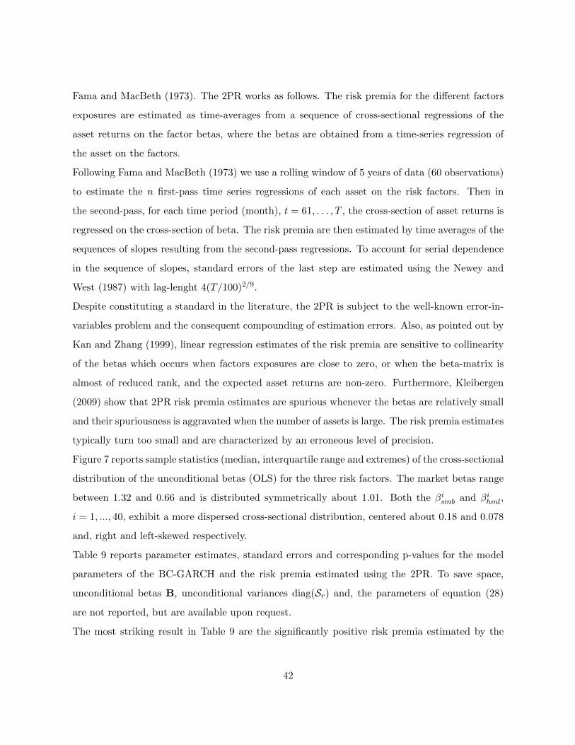
Fama and MacBeth (1973). The 2PR works as follows. The risk premia for the different factors

exposures are estimated as time-averages from a sequence of cross-sectional regressions of the

asset returns on the factor betas, where the betas are obtained from a time-series regression of

the asset on the factors.

Following Fama and MacBeth (1973) we use a rolling window of 5 years of data (60 observations)

to estimate the n first-pass time series regressions of each asset on the risk factors. Then in

the second-pass, for each time period (month), t = 61, . . . , T , the cross-section of asset returns is

regressed on the cross-section of beta. The risk premia are then estimated by time averages of the

sequences of slopes resulting from the second-pass regressions. To account for serial dependence

in the sequence of slopes, standard errors of the last step are estimated using the Newey and

West (1987) with lag-lenght 4(T/100)2/9.

Despite constituting a standard in the literature, the 2PR is subject to the well-known error-in-

variables problem and the consequent compounding of estimation errors. Also, as pointed out by

Kan and Zhang (1999), linear regression estimates of the risk premia are sensitive to collinearity

of the betas which occurs when factors exposures are close to zero, or when the beta-matrix is

almost of reduced rank, and the expected asset returns are non-zero. Furthermore, Kleibergen

(2009) show that 2PR risk premia estimates are spurious whenever the betas are relatively small

and their spuriousness is aggravated when the number of assets is large. The risk premia estimates

typically turn too small and are characterized by an erroneous level of precision.

Figure 7 reports sample statistics (median, interquartile range and extremes) of the cross-sectional

distribution of the unconditional betas (OLS) for the three risk factors. The market betas range

between 1.32 and 0.66 and is distributed symmetrically about 1.01. Both the βismb and βihml,

i = 1, ..., 40, exhibit a more dispersed cross-sectional distribution, centered about 0.18 and 0.078

and, right and left-skewed respectively.

Table 9 reports parameter estimates, standard errors and corresponding p-values for the model

parameters of the BC-GARCH and the risk premia estimated using the 2PR. To save space,

unconditional betas B, unconditional variances diag(Sr) and, the parameters of equation (28)

are not reported, but are available upon request.

The most striking result in Table 9 are the significantly positive risk premia estimated by the

42

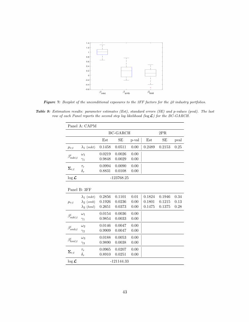
mkt

-0.6

-0.4

-0.2

0

0.2

0.4

0.6

0.8

1

1.2

1.4

smb hml

Figure 7: Boxplot of the unconditional exposures to the 3FF factors for the 40 industry portfolios.

Table 9: Estimation results: parameter estimates (Est), standard errors (SE) and p-values (pval). The lastrow of each Panel reports the second step log likelihood (logL) for the BC-GARCH.

Panel A: CAPM

BC-GARCH 2PR

Est SE p-val Est SE pval

µr,t λ1 (mkt) 0.1458 0.0511 0.00 0.2489 0.2153 0.25

βimkt,tω1 0.0219 0.0026 0.00γ1 0.9848 0.0029 0.00

Σr,tτr 0.0994 0.0090 0.00δr 0.8831 0.0108 0.00

logL -123768.25

Panel B: 3FF

µr,t

λ1 (mkt) 0.2856 0.1101 0.01 0.1824 0.1946 0.34λ2 (smb) 0.1926 0.0236 0.00 0.1801 0.1215 0.13λ3 (hml) 0.2651 0.0373 0.00 0.1475 0.1375 0.28

βimkt,tω1 0.0154 0.0036 0.00γ1 0.9854 0.0033 0.00

βismb,tω2 0.0146 0.0047 0.00γ2 0.9909 0.0047 0.00

βihml,tω3 0.0188 0.0053 0.00γ3 0.9890 0.0038 0.00

Σr,tτr 0.0965 0.0207 0.00δr 0.8910 0.0251 0.00

logL -121144.33

43

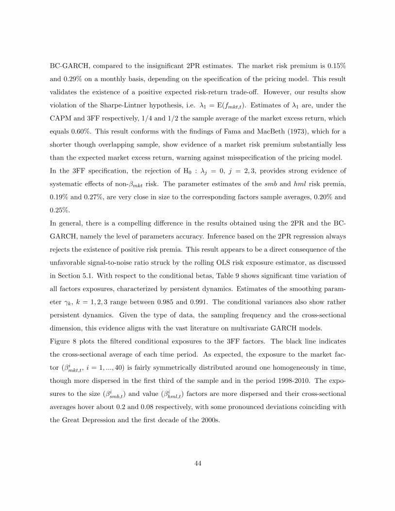
BC-GARCH, compared to the insignificant 2PR estimates. The market risk premium is 0.15%

and 0.29% on a monthly basis, depending on the specification of the pricing model. This result

validates the existence of a positive expected risk-return trade-off. However, our results show

violation of the Sharpe-Lintner hypothesis, i.e. λ1 = E(fmkt,t). Estimates of λ1 are, under the

CAPM and 3FF respectively, 1/4 and 1/2 the sample average of the market excess return, which

equals 0.60%. This result conforms with the findings of Fama and MacBeth (1973), which for a

shorter though overlapping sample, show evidence of a market risk premium substantially less

than the expected market excess return, warning against misspecification of the pricing model.

In the 3FF specification, the rejection of H0 : λj = 0, j = 2, 3, provides strong evidence of

systematic effects of non-βmkt risk. The parameter estimates of the smb and hml risk premia,

0.19% and 0.27%, are very close in size to the corresponding factors sample averages, 0.20% and

0.25%.

In general, there is a compelling difference in the results obtained using the 2PR and the BC-

GARCH, namely the level of parameters accuracy. Inference based on the 2PR regression always

rejects the existence of positive risk premia. This result appears to be a direct consequence of the

unfavorable signal-to-noise ratio struck by the rolling OLS risk exposure estimator, as discussed

in Section 5.1. With respect to the conditional betas, Table 9 shows significant time variation of

all factors exposures, characterized by persistent dynamics. Estimates of the smoothing param-

eter γk, k = 1, 2, 3 range between 0.985 and 0.991. The conditional variances also show rather

persistent dynamics. Given the type of data, the sampling frequency and the cross-sectional

dimension, this evidence aligns with the vast literature on multivariate GARCH models.

Figure 8 plots the filtered conditional exposures to the 3FF factors. The black line indicates

the cross-sectional average of each time period. As expected, the exposure to the market fac-

tor (βimkt,t, i = 1, ..., 40) is fairly symmetrically distributed around one homogeneously in time,

though more dispersed in the first third of the sample and in the period 1998-2010. The expo-

sures to the size (βismb,t) and value (βihml,t) factors are more dispersed and their cross-sectional

averages hover about 0.2 and 0.08 respectively, with some pronounced deviations coinciding with

the Great Depression and the first decade of the 2000s.

44

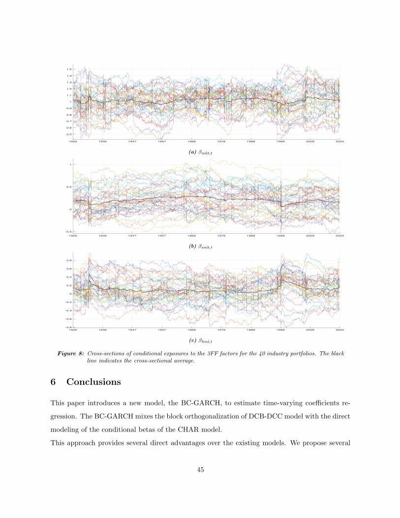
1926 1936 1947 1957 1968 1978 1988 1999 2009 2020

0.5

0.6

0.7

0.8

0.9

1

1.1

1.2

1.3

1.4

1.5

(a) βmkt,t

1926 1936 1947 1957 1968 1978 1988 1999 2009 2020

-0.5

0

0.5

1

(b) βsmb,t

1926 1936 1947 1957 1968 1978 1988 1999 2009 2020

-0.8

-0.6

-0.4

-0.2

0

0.2

0.4

0.6

0.8

(c) βhml,t

Figure 8: Cross-sections of conditional exposures to the 3FF factors for the 40 industry portfolios. The blackline indicates the cross-sectional average.

6 Conclusions

This paper introduces a new model, the BC-GARCH, to estimate time-varying coefficients re-

gression. The BC-GARCH mixes the block orthogonalization of DCB-DCC model with the direct

modeling of the conditional betas of the CHAR model.

This approach provides several direct advantages over the existing models. We propose several

45

conditional beta specifications and derive their theoretical properties (stationarity, invertibility

and, beta tracking). We also propose computationally efficient altrernative QML estimators.

The finite sample properties of the BC-GARCH are studies by means of extensive Monte Carlo

simulations.

We illustrate the usefulness of the BC-GARCH in two empirical applications. The first tests our

model in the context of the linear three factors (market, size and, value) asset pricing frame-

work. The aim of this application is to benchmark a conditional beta specification driven only

by idiosyncratic shocks against three alternatives accounting for different types of beta spillovers.

We consider a bivariate asset system composed by the Coal and Petroleum-Natural Gas value-

weighted industry portfolios tracked over a period spanning from January 1, 1927 to November

30, 2020. Beside time variation in all the conditional betas, we find compelling evidence of both

factor and asset spillovers.

The second empirical application consists of a large scale exercise exploring the cross-sectional

variation of expected returns for 40 industry portfolios. We test a linear conditional beta pric-

ing model and estimate the risk premia attached the market, size and, value exposures. We

benchmark our model against the 2-pass cross-sectional regression approach. We show that our

approach provides a more accurate inference on the risk premia. This is because our model bene-

fits from direct modeling of the time variation in the risk exposures and from the joint estimation

of risk factors exposures and risk premia, avoiding compounding of estimation errors.

References

Aielli, G. P. (2013): “Dynamic Conditional Correlation: On Properties and Estimation,”

Journal of Business and Economic Statistics, 31, 282–299.

Bauwens, L., S. Laurent, and J. V. K. Rombouts (2006): “Multivariate GARCH Models:

A Survey,” Journal of Applied Econometrics, 21, 79–109.

Bollerslev, T. (1990): “Modelling the Coherence in Short-Run Nominal Exchange Rates: A

Multivariate Generalized ARCH Model,” Review of Economics and Statistics, 72, 498–505.

Boussama, F., F. Fuchs, and R. Stelzer (2011): “Stationarity and Geometric Ergodicity

46

of BEKK Multivariate GARCH Models,” Stochastic Processes and their Applications, 121,

2331–2360.

Connor, G. (1984): “A Unified Beta Pricing Theory,” Journal of Economic Theory, 34, 13–31.

Darolles, S., C. Francq, and S. Laurent (2018): “Asymptotics of Cholesky GARCH

Models and Time-Varying Conditional Betas,” Journal of Econometrics, 204, 223–247.

Engle, R. F. (2002): “Dynamic Conditional Correlation: A Simple Class of Multivariate Fen-

eralized Autoregressive Conditional Heteroscedasticity Models,” Journal of Business and Eco-

nomic Statistics, 20, 339–350.

(2016): “Dynamic Conditional Beta,” Journal of Financial Econometrics, 14, 643–667.

Engle, R. F., and K. F. Kroner (1995): “Multivariate Simultaneous Generalized Arch,”

Econometric Theory, 11, 122–150.

Fama, E. F., and K. R. French (1992): “The Cross-Section of Expected Stock Returns,”

Journal of Finance, 47, 427–465.

Fama, E. F., and J. D. MacBeth (1973): “Risk, Return, and Equilibrium: Empirical Tests,”

Journal of Political Economy, 81, 607–636.

Fama, F. F., and R. K. French (1993): “Common Risk Factors in the Returns on Stocks and

Bonds,” Journal of Financial Economics, 33, 3–56.

Fermanian, J.-D., and H. Malongo (2017): “On the Stationarity of Dynamic Conditional

Correlation Models,” Econometric Theory, 33, 636–663.

Francq, C., and J.-M. Zakoian (2012): “QML Estimation of a Class of Multivariate Asym-

metric GARCH Models,” Econometric Theory, 28, 179–206.

(2016): “Estimating Multivariate Volatility Models Equation by Equation,” Journal of

the Royal Statistical Society: Series B (Statistical Methodology), 78, 613–635.

Gonzalez, M., J. Nave, and G. Rubio (2012): “The Cross Section of Expected Returns with

MIDAS Betas,” Journal of Financial and Quantitative Analysis, 47, 115–135.

47

Hafner, C. M., and A. Preminger (2009): “On Asymptotic Theory for Multivariate GARCH

Models,” Journal of Multivariate Analysis, 100, 2044–2054.

Hansen, P. R., A. Lunde, and V. Voev (2014): “Realized Beta GARCH: A Multivariate

GARCH Model with Realized Measures of Volatility,” Journal of Applied Econometrics, 29,

774–799.

Kan, R., and C. Zhang (1999): “Two-Pass Tests of Asset Pricing Models with Useless Factors,”

Journal of Finance, 54, 203–235.

Kleibergen, F. (2009): “Tests of Risk Premia in Linear Factor Models,” Journal of Economet-

rics, 149, 149–173.

Lintner, J. (1965): “Security Prices, Risk, and Maximal Gains from Diversification,” The

Journal of Finance, 20, 587–615.

Newey, W. K., and K. D. West (1987): “A Simple, Positive Semi-definite, Heteroskedasticity

and Autocorrelation Consistent Covariance Matrix,” Econometrica, 55, 703–708.

Pedersen, R. S., and A. Rahbek (2014): “Multivariate Variance Targeting in the

BEKK–GARCH Model,” The Econometrics Journal, 17, 24–55.

Sharpe, W. (1964): “Capital Asset Prices: A Theory of Market Equilibrium Under Conditions

of Risk,” Journal of Finance, 19, 425–442.

48

Research Papers 2021

2020-09: Daniel Borup, Jonas N. Eriksen, Mads M. Kjær and Martin Thyrsgaard: Predicting bond return predictability

2020-10: Alfonso A. Irarrazabal, Lin Ma and Juan Carlos Parra-Alvarez: Optimal Asset Allocation for Commodity Sovereign Wealth Funds

2020-11: Bent Jesper Christensen, Juan Carlos Parra-Alvarez and Rafael Serrano: Optimal control of investment, premium and deductible for a non-life insurance company

2020-12: Anine E. Bolko, Kim Christensen, Mikko S. Pakkanen and Bezirgen Veliyev: Roughness in spot variance? A GMM approach for estimation of fractional log-

normal stochastic volatility models using realized measures

2020-13: Morten Ørregaard Nielsen and Antoine L. Noël: To infinity and beyond: Efficient computation of ARCH(∞) models

2020-14: Charlotte Christiansen, Ran Xing and Yue Xu: Origins of Mutual Fund Skill: Market versus Accounting Based Asset Pricing Anomalies

2020-15: Carlos Vladimir Rodríguez-Caballero and J. Eduardo Vera-Valdés: Air pollution and mobility in the Mexico City Metropolitan Area, what drives the COVID-19 death toll?

2020-16: J. Eduardo Vera-Valdés: Temperature Anomalies, Long Memory, and Aggregation

2020-17: Jesús-Adrián Álvarez, Malene Kallestrup-Lamb and Søren Kjærgaard: Linking retirement age to life expectancy does not lessen the demographic implications of unequal lifespans

2020-18: Mikkel Bennedsen, Eric Hillebrand and Siem Jan Koopman: A statistical model of the global carbon budget

2020-19: Eric Hillebrand, Jakob Mikkelsen, Lars Spreng and Giovanni Urga: Exchange Rates and Macroeconomic Fundamentals: Evidence of Instabilities from Time-Varying Factor Loadings

2021-01: Martin M. Andreasen: The New Keynesian Model and Bond Yields

2021-02: Daniel Borup, David E. Rapach and Erik Christian Montes Schütte: Now- and Backcasting Initial Claims with High-Dimensional Daily Internet Search-Volume Data

2021-03: Kim Christensen, Mathias Siggaard and Bezirgen Veliyev: A machine learning approach to volatility forecasting

2021-04: Fabrizio Iacone, Morten Ørregaard Nielsen and Robert Taylor: Semiparametric Tests for the Order of Integration in the Possible Presence of Level Breaks

2021-05: Stefano Grassi and Francesco Violante: Asset Pricing Using Block-Cholesky GARCH and Time-Varying Betas