Embed Size (px)
Citation preview

Asset Pricing with Imperfect Competition
and Endogenous Market Liquidity
Christoph Heumann
Inauguraldissertation
zur Erlangung des akademischen Grades
eines Doktors der Wirtschaftswissenschaften
der Universitat Mannheim
vorgelegt im Fruhjahrs-/Sommersemester 2007

Dekan: Professor Dr. Hans H. Bauer
Referent: Professor Dr. Wolfgang Buhler
Korreferent: Professor Dr. Ernst-Ludwig von Thadden
Tag der mundlichen Prufung: 20. August 2007

To My Parents


Contents
List of Figures vii
Acknowledgements ix
1 Introduction 1
2 Walrasian Asset Prices and Market Microstructure 7
2.1 The Walrasian Paradigm . . . . . . . . . . . . . . . . . . . . . . . . . 8
2.2 A CARA-Gaussian CAPM . . . . . . . . . . . . . . . . . . . . . . . . 10
2.2.1 Description of the Economy . . . . . . . . . . . . . . . . . . . 11
2.2.2 Walras Equilibrium . . . . . . . . . . . . . . . . . . . . . . . . 12
2.2.3 Equilibrium Properties . . . . . . . . . . . . . . . . . . . . . . 15
2.3 The Myth of the Walrasian Auctioneer . . . . . . . . . . . . . . . . . 18
2.4 Market Liquidity . . . . . . . . . . . . . . . . . . . . . . . . . . . . . 23
2.4.1 Dimensions of Liquidity . . . . . . . . . . . . . . . . . . . . . 24
2.4.2 Determinants of Liquidity . . . . . . . . . . . . . . . . . . . . 27
3 Market Liquidity and Asset Prices: Literature Review 33
3.1 Exogenous Bid-Ask Spreads . . . . . . . . . . . . . . . . . . . . . . . 35
3.1.1 Deterministic Liquidity Effects . . . . . . . . . . . . . . . . . . 35
3.1.2 Liquidity Shocks . . . . . . . . . . . . . . . . . . . . . . . . . 39
3.1.3 Random Time Variations in Liquidity . . . . . . . . . . . . . . 43
3.2 Large Investors . . . . . . . . . . . . . . . . . . . . . . . . . . . . . . 45
3.2.1 Static Models . . . . . . . . . . . . . . . . . . . . . . . . . . . 46
3.2.2 Dynamic Models with a Single Large Investor . . . . . . . . . 48
3.2.3 Dynamic Models with Multiple Large Investors . . . . . . . . 51
v

vi
3.3 Endogenous Market Liquidity . . . . . . . . . . . . . . . . . . . . . . 54
3.4 Discussion . . . . . . . . . . . . . . . . . . . . . . . . . . . . . . . . . 56
4 Asset Prices under Imperfect Competition 61
4.1 Description of the Economy . . . . . . . . . . . . . . . . . . . . . . . 64
4.2 Trading with Imperfect Competition . . . . . . . . . . . . . . . . . . 67
4.3 Equilibrium with Identical Risk Aversion . . . . . . . . . . . . . . . . 73
4.4 Heterogeneity in Risk Aversion . . . . . . . . . . . . . . . . . . . . . 80
4.5 Discussion . . . . . . . . . . . . . . . . . . . . . . . . . . . . . . . . . 88
Appendix: Proofs to Chapter 4 . . . . . . . . . . . . . . . . . . . . . . . . 89
5 Asset Prices with Time-Varying Market Liquidity 97
5.1 Description of the Economy . . . . . . . . . . . . . . . . . . . . . . . 98
5.2 Derivation of Equilibrium Orders . . . . . . . . . . . . . . . . . . . . 101
5.3 Equilibrium Properties in the Basic Scenario . . . . . . . . . . . . . . 104
5.4 Equilibrium Properties in the Signal Scenario . . . . . . . . . . . . . 108
5.5 Discussion . . . . . . . . . . . . . . . . . . . . . . . . . . . . . . . . . 111
Appendix: Proofs to Chapter 5 . . . . . . . . . . . . . . . . . . . . . . . . 112
6 Concluding Remarks 117
References 119

List of Figures
2.1 Price dimensions of market liquidity. . . . . . . . . . . . . . . . . . . 26
3.1 Standard pricing effect of illiquidity. . . . . . . . . . . . . . . . . . . . 58
4.1 Trading against a supply curve. . . . . . . . . . . . . . . . . . . . . . 69
4.2 Market liquidity in the individual trading decision. . . . . . . . . . . 72
4.3 Pricing effect of illiquidity with endogenous trading. . . . . . . . . . . 77
4.4 Trading volume with heterogeneity effect. . . . . . . . . . . . . . . . . 86
5.1 Pricing effect of future illiquidity. . . . . . . . . . . . . . . . . . . . . 107
vii


Acknowledgements
This thesis grew out of my work as a research and teaching assistant at the Chair
of Finance at the University of Mannheim; it was accepted as dissertation by the
Faculty of Business Administration.
Acknowledgements are due to many. First, I am obliged to thank my advisor
Prof. Dr. Wolfgang Buhler for many comments that helped to improve this thesis.
I would also like to thank my second advisor Prof. Dr. Ernst-Ludwig von Thadden
for co-refereeing the thesis. Many thanks go to my current and former colleagues at
the Chair of Finance, namely Martin Birn, Jens Daum, Christoph Engel, Sebastian
Herzog, Prof. Dr. Olaf Korn, Dr. Christian Koziol, Jens Muller-Merbach, Stephan
Pabst, Raphael Paschke, Marcel Prokopczuk, Dr. Peter Sauerbier, Dr. Antje Schirm,
Christian Speck, Volker Sygusch, Dr. Tim Thabe, Monika Trapp, Volker Vonhoff,
as well as our secretary Marion Baierlein; they provided a friendly and stimulating
environment to work in.
Most of all, I thank my family—my parents Herbert and Frieda and my brother
Dietmar. Their unfailing support throughout the years made this thesis possible.
Mannheim, September 2007 Christoph Heumann
ix


Chapter 1
Introduction
The equilibrium expected return, or the required return, on financial assets is a cen-
tral variable in financial economics, and understanding the determinants of required
asset returns is the fundamental goal of asset pricing. The basic insight of traditional
neoclassical asset pricing models is that the equilibrium expected return of an asset
is increasing in the systematic risk of the asset, as risk-averse investors require com-
pensation for bearing non-diversifiable risk. Neoclassical models, however, are based
on the assumption that markets for financial assets are frictionless. Accordingly,
trade in these markets is regarded as costless, and the actual process of trading and
price formation is, in fact, left unmodeled. The starting point of this thesis is that
real-world financial markets are not frictionless and that trading of financial assets
can involve considerable costs. This raises the question of how market frictions affect
required asset returns.
A market friction of major importance to investors is a lack of market liquidity.
Roughly stated, market liquidity refers to the ease of trading financial assets, with
more liquid markets having lower trading costs. Trading costs in illiquid markets
include execution costs in the form of commissions, bid-ask spreads, and price im-
pact, and also opportunity costs in the form of delayed and uncompleted trades. The
effects of such costs on investment performance are often measured by the imple-
mentation shortfall proposed by Perold (1988), and these effects can be surprisingly
large. For instance, Perold (1988) shows that a hypothetical “paper” portfolio based
on the weekly stock recommendations of the Value Line Investment Survey has out-
1

2 1. Introduction
performed the market by almost 20% per year over the period from 1965-1986, while
the corresponding real portfolio of the Value Line Fund has outperformed the market
by only 2.5% per year—the difference representing the implementation shortfall.
When trading costs are important to investors, then a lack of market liquidity may
also affect required asset returns. The standard result here traces back to Amihud and
Mendelson (1986), who show that trading costs in illiquid markets reduce the price
of an asset and, equivalently, increase the equilibrium expected return of an asset, as
investors require compensation for bearing these costs. Hence, required asset returns
should reflect both a risk premium as compensation for risk and a liquidity premium
as compensation for illiquidity.
This pricing effect of illiquidity has become the conventional wisdom on the role
of market frictions in asset pricing. For instance, Stoll (2000, p. 1483) argues that
“frictions must be reflected in lower asset prices so that the return on an asset is
sufficient to offset the real cost of trading the asset, adjusted for the holding period.”
Following this line of argument, a simple back-of-the-envelope example illustrates the
effect. For stocks on the New York Stock Exchange, the average effective bid-ask
spread is approximately 2.2% and the average turnover of the outstanding shares
is approximately 60% on an annual basis. Ignoring trading costs other than bid-
ask spreads, these numbers suggest that the average required stock return should be
increased by a liquidity premium of about 0.6 · 2.2% = 1.3%, which in turn would
have a large effect on the level of stock prices.1
Market liquidity is an elusive concept, however, and how exactly illiquidity af-
fects required asset returns remains a subject of considerable controversy and debate.
As O’Hara (2003) points out, the principal difficulty for understanding the precise
relationship between market liquidity and required asset returns is the separation
of the related fields of research into asset pricing and market microstructure. Asset
pricing, on the one hand, studies the macro determinants of asset prices, but gives
only a limited representation of the underlying market interactions among investors.
For example, asset pricing models in the line of Amihud and Mendelson (1986) just
take trading costs as given and enforce trade among investors by imposing exogenous
1The example is taken from Garleanu and Pedersen (2004) with numbers on NYSE stocks from
Chalmers and Kadlec (1998).

1. Introduction 3
life-cycle motives. Market microstructure, on the other hand, analyzes (among other
things) the determinants of trading costs based on a deeper view on the trading and
price formation process, but does not consider the broader level of asset prices. For
example, microstructure models examine how adverse selection problems among mar-
ket participants affect the size of a bid-ask spread rather than where the level of the
asset price and the spread is in the first place. O’Hara (2003, p. 1335) summarizes,
“asset pricing ignores the central fact that market microstructure focuses on: asset
prices evolve in markets,” and highlights the need for a linkage of asset pricing and
market microstructure in order to improve the understanding of how microstructure
variables such as market liquidity affect equilibrium expected asset returns.
The contribution of this thesis is to study the role of market liquidity in asset
pricing within a theoretical framework that integrates the asset pricing and the mar-
ket microstructure view. Our framework allows to derive market liquidity, investors’
trading behavior, and required asset returns endogenously and, hence, to analyze the
pricing effect of illiquidity on the basis of an explicit microstructure foundation. We
employ a CARA-Gaussian asset pricing setup with a single risky asset and incor-
porate market liquidity by allowing for imperfect competition. Investors trade by
submitting demand functions for execution against each other, and each investor rec-
ognizes that he faces trading costs in the form of price impact, arising endogenously
from the demand functions of the other agents. The resulting equilibrium is thus
a Nash equilibrium in demand functions as in Kyle’s (1989) noisy rational expecta-
tions model on information aggregation with imperfect competition. However, we use
the framework in an asset pricing context, with investors trading under symmetric
information to improve risk sharing.
Our results on market liquidity are consistent with the inventory-based strand of
the microstructure literature. We find that investors’ risk aversion and strategic trad-
ing behavior impair market liquidity and thereby generate trading costs. Investors
respond to this lack of market liquidity by restricting trading volume in order to
reduce their execution costs. As a consequence, investors incur opportunity costs, as
their portfolio holdings of the risky asset do not achieve Pareto-optimal risk sharing.
Our main result is, however, that illiquidity does not affect the price and the
required return of the risky asset. The reason is the endogeneity of trading behavior
4 1. Introduction
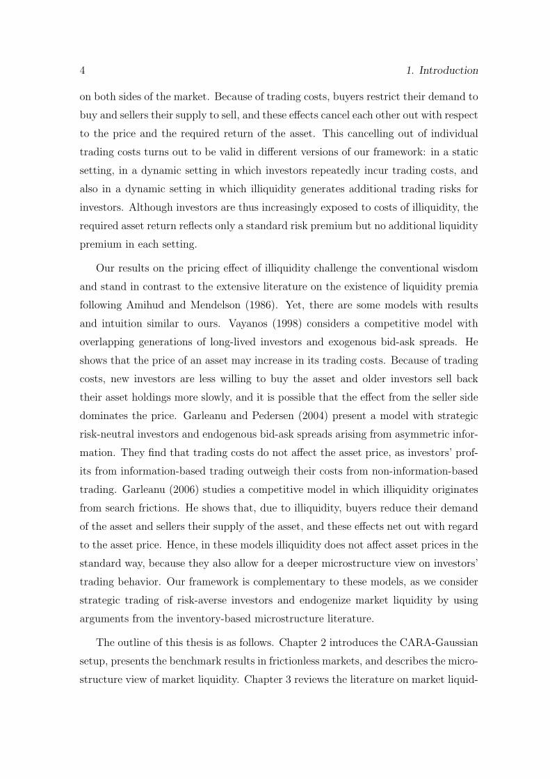
on both sides of the market. Because of trading costs, buyers restrict their demand to
buy and sellers their supply to sell, and these effects cancel each other out with respect
to the price and the required return of the asset. This cancelling out of individual
trading costs turns out to be valid in different versions of our framework: in a static
setting, in a dynamic setting in which investors repeatedly incur trading costs, and
also in a dynamic setting in which illiquidity generates additional trading risks for
investors. Although investors are thus increasingly exposed to costs of illiquidity, the
required asset return reflects only a standard risk premium but no additional liquidity
premium in each setting.
Our results on the pricing effect of illiquidity challenge the conventional wisdom
and stand in contrast to the extensive literature on the existence of liquidity premia
following Amihud and Mendelson (1986). Yet, there are some models with results
and intuition similar to ours. Vayanos (1998) considers a competitive model with
overlapping generations of long-lived investors and exogenous bid-ask spreads. He
shows that the price of an asset may increase in its trading costs. Because of trading
costs, new investors are less willing to buy the asset and older investors sell back
their asset holdings more slowly, and it is possible that the effect from the seller side
dominates the price. Garleanu and Pedersen (2004) present a model with strategic
risk-neutral investors and endogenous bid-ask spreads arising from asymmetric infor-
mation. They find that trading costs do not affect the asset price, as investors’ prof-
its from information-based trading outweigh their costs from non-information-based
trading. Garleanu (2006) studies a competitive model in which illiquidity originates
from search frictions. He shows that, due to illiquidity, buyers reduce their demand
of the asset and sellers their supply of the asset, and these effects net out with regard
to the asset price. Hence, in these models illiquidity does not affect asset prices in the
standard way, because they also allow for a deeper microstructure view on investors’
trading behavior. Our framework is complementary to these models, as we consider
strategic trading of risk-averse investors and endogenize market liquidity by using
arguments from the inventory-based microstructure literature.
The outline of this thesis is as follows. Chapter 2 introduces the CARA-Gaussian
setup, presents the benchmark results in frictionless markets, and describes the micro-
structure view of market liquidity. Chapter 3 reviews the literature on market liquid-

1. Introduction 5
ity in asset pricing. Chapter 4 presents our static asset pricing setting with imperfect
competition and endogenous market liquidity, and Chapter 5 extends the analysis to
settings with dynamic and stochastic trading effects. Chapter 6 contains concluding
remarks.


Chapter 2
Walrasian Asset Prices and Market
Microstructure
Asset pricing theory has many of its foundations in the neoclassical paradigm of gen-
eral equilibrium analysis in the tradition of the early works of Walras (1874), Pareto
(1909), and Fisher (1930), and their extensions to models with time and uncertainty
by Arrow (1953) and Debreu (1959). The basic view of the neoclassical paradigm is
that self-interested agents meet in frictionless markets where their competitive and
independent actions are coordinated by the price mechanism, so that mutually bene-
ficial trade takes place. The actual process of price formation is not made explicit,
however, but is attributed to the impersonal forces of the market in the spirit of
Adam Smith’s (1776) “invisible hand.”
The question of how prices are formed is addressed in market microstructure
theory. Its focus is on the interrelations between market frictions, institutional market
rules, and strategic interactions among agents. In order to analyze the effects of
frictions and strategic trading on equilibrium asset returns, it is therefore promising
to integrate market microstructure features into asset pricing theory.
In this chapter, we provide the building blocks for our analysis of asset pricing
with imperfect competition and endogenous market liquidity. Section 2.1 reviews
the assumptions that constitute the neoclassical paradigm of frictionless markets.
Section 2.2 presents a standard neoclassical asset pricing model, which serves as ref-
erence point and as workhorse model for subsequent chapters. Section 2.3 discusses
the neoclassical view on the price formation process; a special emphasis is given to
7

8 2. Walrasian Asset Prices and Market Microstructure
the absence of strategic interactions among agents, which is implied by the neoclas-
sical assumption of perfect competition. Finally, Section 2.4 describes the market
microstructure concept of market liquidity in detail.
2.1 The Walrasian Paradigm
Almost all of the issues addressed in neoclassical finance can be traced back to
two independent key ideas: first, the concept of no-arbitrage introduced by Keynes
(1923, ch. 3) relating to the interest rate parity theory of foreign exchange rates and
by Modigliani and Miller (1958) in the context of optimal corporate capital structure;
and second, the theory of portfolio selection developed by Markowitz (1952, 1959)
and Tobin (1958). Based upon these elementary principles, some of the most seminal
contributions in the theory of asset pricing (the subfield of finance that is concerned
with the valuation of financial securities and derivatives) are the static capital as-
set pricing model (CAPM) by Treynor (1961), Sharpe (1964), Lintner (1965), and
Mossin (1966), its extensions to dynamic settings by Merton (1973a) and Breeden
(1979), the arbitrage pricing theory by Ross (1976), the theory of derivatives pricing
by Black and Scholes (1973) and Merton (1973b), and the connection of asset prices
to the production technology in the economy by Cox, Ingersoll, and Ross (1985a,
1985b).
The features that are common to neoclassical asset pricing models and that ba-
sically constitute the paradigm of neoclassical equilibrium analysis (hereafter also
referred to as “Walrasian paradigm”) are the assumptions about the economy and
the conditions for equilibrium. In the following, these features are described in detail.
The focus thereby is on models on absolute pricing, in which all securities are valued
endogenously according to investors’ endowments, preferences, and information—in
contrast to models on relative pricing, in which some assets are valued in terms of ex-
ogenous prices of related assets. Furthermore, the description aims at asset pricing in
secondary financial markets for the case that investors trade a given stock of outstand-
ing securities motivated by risk sharing and that asset payoffs from firms’ underlying
production activities are exogenous. The following combination of assumptions is
characteristic for the Walrasian paradigm.

2.1. The Walrasian Paradigm 9
Perfect Competition: Each investor acts as price taker, i.e., each investor decides
on his individual trading actions as if his actions do not affect the resulting prices.
The assumption of price-taking behavior is usually motivated as a reasonable approxi-
mation to situations when there is a large number of investors in the market and each
investor is small relative to the rest of the market.1
Perfect Capital Markets: Every asset can be traded without costs and without
delay at any instant in time. There are no taxes. Assets are perfectly divisible, and
short selling is allowed without restrictions. Prices are freely observable and identical
for all investors.
Symmetric Information: No investor has an informational advantage over any
other agent, and all investors have identical information about asset payoffs (ho-
mogenous expectations). Each investor knows his own characteristics (endowments,
preferences), but does not observe the characteristics of the other agents.
Rational Investors: Each investor decides on his individual trading actions with
the objective to maximize his utility, given his endowments and information. In-
vestors derive utility from lifetime consumption of a single consumption good or, as
assumed in the following, from terminal wealth. For decisions under uncertainty, each
investor is risk averse and makes his decision on the basis of mean and variance of ter-
minal wealth. Consistency of mean-variance preferences with the standard expected
utility approach in the von Neumann-Morgenstern sense can be assured by assuming
quadratic utility functions or by assuming normally distributed terminal wealth.2
Given this combination of assumptions, a neoclassical equilibrium (“Walras equi-
librium”) is defined by the conditions that (i) each investor selects an optimal port-
folio of assets, and (ii) prices are determined such that all markets clear. As the
Walrasian paradigm studies market outcomes in completely frictionless markets, it
provides a useful benchmark for the analysis of asset prices under more realistic con-
ditions where trading costs and other market frictions interfere with the actions of
investors.
1Aumann (1964) shows that the effect of each individual agent on prices becomes mathematically
negligible when agents are represented as points in a continuum.2See Ingersoll (1987, ch. 4) or Huang and Litzenberger (1988, ch. 3).

10 2. Walrasian Asset Prices and Market Microstructure
2.2 A CARA-Gaussian CAPM
The CAPM is the most prominent neoclassical asset pricing model and a cornerstone
of modern finance. It provides an equilibrium analysis of the prices of risky assets and
the structure of investors’ portfolio holdings.3 In this section, we present the CAPM
in a static CARA-Gaussian version, which serves as a reference point and a workhorse
model for the analysis in subsequent chapters. In a static model, each agent acts only
once and all agents act at the same time. Thus, all investors meet in a single round
of trading and thereafter simply hold their portfolios, receive terminal asset payoffs,
and then consume their terminal wealth. Furthermore, the CARA-Gaussian setting
places restrictions on investor preferences and asset payoffs. If wi denotes terminal
wealth to be consumed by investor i, then the following two assumptions are made.
• Each investor i has a negative exponential (CARA) utility function over ter-
minal wealth, ui (wi) = −exp (−ρiwi), with a constant Arrow-Pratt index of
absolute risk aversion,
−∂2ui/∂ (wi)
2
∂ui/∂wi= ρi.
The inverse of the absolute risk aversion measure is referred to as risk tolerance.
The CARA utility function belongs to the class of utility functions for which
risk tolerance is linear in wealth (also called hyperbolic absolute risk aversion
(HARA) utility functions),
−∂ui/∂wi
∂2ui/∂ (wi)2= ai + biwi. (2.1)
Clearly, CARA utility satisfies condition (2.1) with ai = 1/ρi and bi = 0.
• The payoffs of all risky assets are jointly normally distributed (Gaussian), and
terminal wealth generated by the portfolio of investor i is thus also normally
distributed, wi ∼ N (E [wi] ,Var [wi]).
3The assessment of the validity of the CAPM remains controversial, however; Jagannathan and
McGrattan (1995) and Fama and French (2004) summarize the debate on the CAPM.

2.2. A CARA-Gaussian CAPM 11
With exponential utility and normally distributed wealth, the expected utility func-
tion over wealth becomes4
E[ui(wi)]
=1
√
2πVar [wi]
∫ ∞
−∞
−exp
[
−
(
ρiwi +(wi − E [wi])
2
2Var [wi]
)]
dwi
= −exp
[
−ρi
(
E[wi]−ρi
2Var
[wi])]
.
Maximizing expected utility is thus equivalent to maximizing the mean-variance ob-
jective function E [wi] − ρiVar [wi] /2.
The main motivation for the CARA-Gaussian framework is analytical tractability,
which allows us to obtain closed-form solutions and to trace asset prices back to
their underlying economic determinants. Furthermore, the resulting linear demand
functions will be crucial for the analysis of strategic interactions among investors as
carried out in later chapters of this thesis. The drawbacks of the setting are that
(i) exponential utility implies that—when rates of returns on assets are given and
riskless borrowing and lending is possible without restrictions—an investor’s demand
for risky assets does not depend on his initial wealth, and (ii) normally distributed
payoffs can become negative with strictly positive probability and have unlimited
downside liability. Both properties may be questioned regarding their descriptive
realism.
The CARA-Gaussian version of the standard CAPM goes back to Lintner (1970).
In the following, we briefly review the model and its main results; as the results are
well-known, proofs are omitted.5
2.2.1 Description of the Economy
We consider a static framework with two risky assets (indexed by k = 1, 2) and a
riskless asset. At the beginning of the period, assets are traded among investors with
pk denoting the price of risky asset k and pf the price of the riskfree asset. At the
end of the period, assets pay off exogenous liquidation values, and investors consume
4The proof can be found in Sargent (1987, pp. 154-5).5Stapleton and Subrahmanyam (1978) extend the CARA-Gaussian framework to a dynamic
CAPM. Lintner (1969) is an early application of the setting to a CAPM with heterogeneous expec-
tations. Bamberg (1986) gives a detailed discussion of the economic rationale of the CARA-Gaussian
approach. For presentations of standard asset pricing theory in more general settings, see e.g. In-
gersoll (1987), Huang and Litzenberger (1988), LeRoy and Werner (2001), or Cochrane (2005).

12 2. Walrasian Asset Prices and Market Microstructure
their terminal wealth. The per-share payoff of each risky asset k is given by vk, where
the vk are normally distributed with mean E [vk] and covariance Cov [v1, v2]. Each
unit of the riskfree asset yields a payoff R. The total number of outstanding shares
of risky asset k and of the riskless asset is denoted by Xk and Y , respectively.
In the economy, there are I rational investors (indexed by i = 1, 2, . . . , I) with
homogenous expectations about asset payoffs. Each investor i is initially endowed
with yi units of the riskless asset and xik units of risky asset k (where
∑I
i=1yi ≡ Y
and∑I
i=1xi
k ≡ Xk) and hence has initial wealth
wi = pf yi + p1x
i1 + p2x
i2.
If yi and xik are the corresponding portfolio holdings after trade has taken place, then
investor i’s terminal wealth follows as
wi = Ryi + v1xi1 + v2x
i2.
Each agent has a CARA utility function with a coefficient of absolute risk aversion
ρi > 0. As terminal wealth is normally distributed, the objective for each investor is
to choose his portfolio holdings to maximize
Πi(yi, xi
1, xi2
):= E
[wi]−ρi
2Var
[wi]
subject to his budget constraint. Each investor takes the prices of all assets as given,
and markets for all assets are perfect.
2.2.2 Walras Equilibrium
To make the concept of Walras equilibrium formal, let I = 1, 2, . . . , I denote the
set of investors, (yi, xi1, x
i2) the initial endowments and Πi the objective function for
investor i, and let E =I, (yi, xi
1, xi2) ,Π
ii∈I
denote the associated economy to be
studied. Furthermore, denote by (yi, xi1, x
i2) the asset holdings of investor i after trade
has taken place, by (yi, xi1, x
i2)i∈I
an allocation of assets among investors, and by
(pf , p1, p2) a system of prices. Then we have the following definition.
Definition 1 A Walras equilibrium of economy E is an allocation(yi,∗, xi,∗
1 , xi,∗2
)
i∈I
and a price system(p∗f , p
∗1, p
∗2
)such that the following conditions are satisfied:
2.2. A CARA-Gaussian CAPM 13
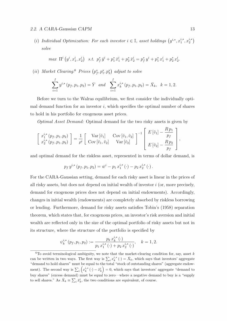
(i) Individual Optimization: For each investor i ∈ I, asset holdings(yi,∗, xi,∗
1 , xi,∗2
)
solve
max Πi(yi, xi
1, xi2
)s.t. p∗f y
i + p∗1 xi1 + p∗2 x
i2 = p∗f y
i + p∗1 xi1 + p∗2 x
i2.
(ii) Market Clearing:6 Prices(p∗f , p
∗1, p
∗2
)adjust to solve
I∑
i=1
yi,∗ (pf , p1, p2) = Y andI∑
i=1
xi,∗k (pf , p1, p2) = Xk, k = 1, 2.
Before we turn to the Walras equilibrium, we first consider the individually opti-
mal demand function for an investor i, which specifies the optimal number of shares
to hold in his portfolio for exogenous asset prices.
Optimal Asset Demand: Optimal demand for the two risky assets is given by
[xi,∗
1 (pf , p1, p2)
xi,∗2 (pf , p1, p2)
]
=1
ρi
[Var [v1] Cov [v1, v2]
Cov [v1, v2] Var [v2]
]−1
E [v1] −Rp1
pf
E [v2] −Rp2
pf
,
and optimal demand for the riskless asset, represented in terms of dollar demand, is
pf yi,∗ (pf , p1, p2) = wi − p1 x
i,∗1 (·) − p2 x
i,∗2 (·) .
For the CARA-Gaussian setting, demand for each risky asset is linear in the prices of
all risky assets, but does not depend on initial wealth of investor i (or, more precisely,
demand for exogenous prices does not depend on initial endowments). Accordingly,
changes in initial wealth (endowments) are completely absorbed by riskless borrowing
or lending. Furthermore, demand for risky assets satisfies Tobin’s (1958) separation
theorem, which states that, for exogenous prices, an investor’s risk aversion and initial
wealth are reflected only in the size of the optimal portfolio of risky assets but not in
its structure, where the structure of the portfolio is specified by
ψi,∗k (pf , p1, p2) :=
pk xi,∗k (·)
p1 xi,∗1 (·) + p2 x
i,∗2 (·)
, k = 1, 2.
6To avoid terminological ambiguity, we note that the market-clearing condition for, say, asset k
can be written in two ways. The first way is∑
i xi,∗k (·) = Xk, which says that investors’ aggregate
“demand to hold shares” must be equal to the total “stock of outstanding shares” (aggregate endow-
ment). The second way is∑
i
(
xi,∗k (·) − xi
k
)
= 0, which says that investors’ aggregate “demand to
buy shares” (excess demand) must be equal to zero—where a negative demand to buy is a “supply
to sell shares.” As Xk ≡∑
i xik, the two conditions are equivalent, of course.

14 2. Walrasian Asset Prices and Market Microstructure
Thus, the problem of optimal asset demand can be separated into a two-stage process:
first, selecting the optimal structure of the portfolio of risky assets; and second,
determining how much wealth to invest into risky assets overall and how much to
borrow or lend at the riskless rate of interest. Under Tobin separation, only the
second step of the demand decision depends on individual investor characteristics.
Hence, the first step of the decision can be made independently of the specific investor
characteristics and also independently of the second step.7
Now we turn to the Walras equilibrium of the economy. Allingham (1991) and
Hens, Laitenberger, and Loffler (2002) show that both the joint assumptions of CARA
utility and normally distributed payoffs (without assumption on the presence of a
riskless asset) and the joint assumptions of CARA utility and presence of a risk-
less asset (without assumption on payoff distributions) are sufficient to guarantee a
unique equilibrium in the CAPM. Hence, a unique equilibrium does also exist in the
economy E to be studied here.
Equilibrium Prices: Equilibrium prices of economy E are
p∗kp∗f
=1
R
(
E [vk] −Cov
[vk, v1X1 + v2X2
]
∑I
i=1(1/ρi)
)
, k = 1, 2. (2.2)
The price of a risky asset is given by the expected payoff of the asset minus a risk
premium, discounted at the riskfree rate of interest. The risk premium, in turn,
is determined as the covariance of the per-share payoff of that asset with the total
payoff of all risky assets in the economy, divided by the aggregate risk tolerance of
the economy. As all investors obey their budget constraints as an accounting identity,
market clearing for all but one market implies market clearing also for the remaining
market (Walras’ law). As a consequence, it is possible to determine prices only for all
but one asset in relation to the remaining asset (numeraire asset). In the following,
we choose the riskless asset as numeraire (i.e., we set pf = 1) and denote the riskless
rate of interest by r := R/pf − 1 = R− 1.
7Hakansson (1969) and Cass and Stiglitz (1970) show that, in the presence of a riskless asset,
Tobin separation holds (under more general payoff distributions than the Gaussian), if and only if
the investor has a utility function with linear risk tolerance.

2.2. A CARA-Gaussian CAPM 15
Equilibrium Allocation: The equilibrium allocation of economy E is
xi,∗k =
(1/ρi)∑I
i=1(1/ρi)
Xk for all i and all k, (2.3)
yi,∗ = yi + p∗1 xi1 + p∗2 x
i2 − p∗1 x
i,∗1 − p∗2 x
i,∗2 for all i. (2.4)
All outstanding risky assets are allocated among investors according to the proportion
of each individual investor’s risk tolerance to the aggregate risk tolerance of the
economy. The portfolio holdings of the riskless asset simply absorb the remaining
wealth not invested into risky assets; thus, we skip the closed-form representation for
the riskless holdings.
Prices (2.2) and allocation (2.3) and (2.4) constitute the unique Walras equilib-
rium of economy E . In the next subsection, we review the main properties of this
equilibrium.
2.2.3 Equilibrium Properties
Here we describe the main properties of the Walras equilibrium of economy E .8 Sev-
eral of these properties do not hold in more general settings of the incomplete-markets
economy of the CAPM, but are known to hold for economies that are at least effec-
tively complete. Rubinstein (1974) provides sets of sufficient conditions for effective
completeness. In particular, effectively complete economies encompass economies
that fulfill the following three conditions: (i) a riskless asset exists; (ii) all endow-
ments are tradable; and (iii) all investors have utility functions with linear risk tol-
erance (as in (2.1)) and with identical coefficients of marginal risk tolerance (bi = b
for all i). The conditions (i) − (iii) are satisfied by economy E to be studied here.9
Mutual Fund Theorem: For each investor i, the structure of the risky asset port-
folio is given by
ψik :=
pk xik
p1xi1 + p2xi
2
=E [vk] Xk
∑I
i=1(1/ρi) − Cov
[vkXk, v1X1 + v2X2
]
(E [v1] X1 + E [v2] X2
)∑I
i=1(1/ρi) − Var
[v1X1 + v2X2
] , k = 1, 2. (2.5)
8As all properties refer to equilibrium, we drop the stars on endogenous variables for notational
simplicity.9Geanakoplos and Shubik (1990) examine the CAPM in a much more general framework of a
full-blown general equilibrium model with incomplete markets.

16 2. Walrasian Asset Prices and Market Microstructure
Equation (2.5) reveals that the structure of each investor’s portfolio of risky assets
depends on the individual risk preferences of all agents, but for all investors in the
same way (on the aggregate risk tolerance of the economy). Thus, we have
ψik = ψk for all i and all k,
i.e., the structure of risky asset holdings is the same for all investors, even if investors
differ in individual risk aversion or initial wealth. It is as if all risky assets were
arranged in a single mutual fund, each risky asset with the proportion ψk, and each
investor holds a fraction of this fund. Rubinstein (1974) shows that conditions (i) −
(iii) are sufficient for the mutual fund theorem to hold.
Market Portfolio: An important insight of the CAPM is that the pricing-relevant
risk of an asset is not given by the variance of its payoff but rather by the covariance
of its payoff with the payoff of a particular portfolio that contains all risky assets of
the economy. The pricing-relevant risk is called systematic risk, and the particular
portfolio is called market portfolio. If the structure of the market portfolio is denoted
by
Ψk :=pkXk
p1X1 + p2X2
, k = 1, 2,
then we have
Ψk = ψk, k = 1, 2.
Hence, the structure of the market portfolio coincides with the structure of the risky
asset portfolio of each investor. This is the case, as all investors have the same optimal
structure of risky asset holdings and all investors hold all outstanding risky assets in
their portfolios altogether. The structure of the market portfolio is mean-variance
efficient, i.e., risky asset portfolios with this structure (held alone or combined with
riskless borrowing or lending) have maximum expected return for a given level of risk.
If the payoff and the price of the market portfolio are denoted by VM := v1X1 + v2X2
and PM := p1X1 + p2X2, respectively, then
Λ :=E[
VM
]
− (1 + r)PM
Var[
VM
] =
(I∑
i=1
(1/ρi)
)−1
(2.6)

2.2. A CARA-Gaussian CAPM 17
is Lintner’s (1970) version of the market price of (dollar) risk. The market price of
risk in the CARA-Gaussian setting is thus equal to the inverse of the aggregate risk
tolerance of the economy.10
Pareto Optimality (Pareto Efficiency): The allocation of assets among investors
is Pareto optimal, i.e., it is not possible to redistribute assets to make some investor
strictly better off without making some other investor strictly worse off. That the
risk-tolerance-weighted allocation rule in (2.3) provides the unique Pareto-optimal al-
location for the risky assets is known from the analysis of risk sharing among groups
by Wilson (1968); accordingly, the Pareto-optimal allocation is also referred to as
optimal (efficient) risk sharing. However, that the Pareto-optimal allocation is es-
tablished in the CAPM is not self-evident, as Pareto optimality for Walras equilibria
from the first welfare theorem requires a complete-markets economy. With incom-
plete markets, in contrast, the allocation is not Pareto optimal in general, but only
in certain special cases. Rubinstein (1974) shows that conditions (i) − (iii) are suf-
ficient for Pareto optimality to be achieved in incomplete-market economies. Thus,
Pareto optimality holds for the economy E studied here. The establishing of Pareto
optimality within the single round of trading in the static CAPM implies that, even
10The more familiar version of the CAPM using rates of returns rather than prices can now
be obtained as follows. First, let the return on an asset (or on a portfolio of assets) be denoted
r := v/p − 1, such that
E [vk] = pk (1 + E [rk]) , (2.7)
Cov [vk, vj ] = pkpjCov [rk, rj ] . (2.8)
Next, a more standard version of the market price of risk is defined by Λ′ := ΛPM and can be
derived by rewriting (2.6) and using (2.7) and (2.8) to obtain
Λ′ =
(
E[
VM
]
− (1 + r)PM
)
P 2
M
PM Var[
VM
] =E [rM ] − r
Var [rM ]. (2.9)
Finally, the standard security market line can be derived by substituting (2.7) and (2.8) into (2.2)
and using (2.6) and (2.9) to obtain
E [rk] = r +(E [rM ] − r) Cov [rk, rM ]
Var [rM ], k = 1, 2. (2.10)
Note that (2.9) is not an explicit (closed-form) solution for the market price of risk (as rM depends on
the prices of all risky assets), and hence the security market line (2.10) and all other pricing relations
based upon (2.9) are also merely implicit representations. For a comparative static analysis of the
market price of risk for other utility functions than the exponential, see Rubinstein (1973).

18 2. Walrasian Asset Prices and Market Microstructure
if markets were re-opened at later dates for additional rounds of trading among the
same investors (as in a dynamic model), no additional trades would occur, as there
is no potential for additional mutually beneficial trading left.
Representative Investor: As the allocation of assets is Pareto optimal, asset prices
in economy E are the same as in an economy with a single, suitably constructed repre-
sentative investor. Deriving asset prices via a representative agent economy provides
a means of analytical simplification.11 In general, however, the construction of the
representative agent depends on the initial distribution of endowments among in-
vestors in the underlying economy. Hence, redistributions of endowments change the
characteristics of the representative agent and also change asset prices. Once again,
Rubinstein (1974) shows that conditions (i) − (iii) are sufficient to have an excep-
tional case where representative agent and asset prices are independent of the initial
distribution of endowments among investors (aggregation property). In particular,
the representative investor for the CARA-Gaussian economy E is characterized by
the risk tolerance 1/ρrepr =∑I
i=1(1/ρi).
To conclude the discussion, we note that the sufficiency of Rubinstein’s (1974)
conditions (i)− (iii) for several of the above equilibrium properties relies on the fric-
tionless setting of the Walrasian paradigm. That is, mutual fund theorem, Pareto
optimality, and representative investor pricing with aggregation property do not nec-
essarily carry over to economics that satisfy (i) − (iii), but exhibit trading costs or
other market frictions.
2.3 The Myth of the Walrasian Auctioneer
In the Walrasian paradigm, which underpins neoclassical asset pricing and which also
underpins neoclassical economics as best represented by the Arrow-Debreu model of
general equilibrium (GE), prices play a crucial role: prices equate demand and supply
on all markets and reflect the various marginal rates of substitution; prices are freely
observable and summarize all relevant information needed by agents in order to decide
what their optimal actions are; and prices are the coordinating force that aligns the
11Note that representative investor analysis provides a simplified pricing technique, but is not to
be taken literally, of course. If there were de facto only a single investor, then there could not be
trade and hence there would be no need for prices (i.e. trading ratios) in the first place.

2.3. The Myth of the Walrasian Auctioneer 19
competitive and independent actions of the different agents, so that mutually welfare-
increasing trade can take place.
What is missing in the Walrasian paradigm, however, is an explicit mechanism by
which these prices are established. While prices are derived analytically by solving a
simultaneous equation system for the economy—and conditions under which such a
solution exists have been examined with considerable mathematical effort and rigor—
it remains unspecified who or what, exactly, in the economy enforces this system of
prices and how neoclassical equilibrium is actually attained. Accordingly, neoclassical
models point out the logical possibility of equilibrium existence, but do not show how,
or if, equilibrium will actually be reached on the basis of any price formation process
in the market. Yet, the question of how equilibrium is established is important in at
least two respects.
First, the abstraction from an explicit price mechanism involves the implicit as-
sumption that, whatever mechanism is actually employed, it has no effect on the
market outcomes to be studied. Similarly, potential frictions associated with the
actual price mechanism are also assumed to have no effects on the outcomes of the
market. This aspect provides the focus for the asset pricing analysis in subsequent
chapters of this thesis. The main question will be: how do frictions in the trading
and price formation process affect the equilibrium expected return on risky assets,
when investors interact under an explicit set of market rules?
Second, the abstraction from an explicit price mechanism is important from a
methodological point of view. The ultimate purpose for studying equilibrium models
is, of course, to gain understanding of causal relations between economic variables in
the real world. This approach is based on the premise that the variables in the real
world will ultimately reach, or at least gravitate towards, the equilibrium state of the
model. As pointed out by von Hayek (1937, p. 44), “it is only with this assertion
[of a tendency to equilibrium] that economics ceases to be an exercise in pure logic
and becomes an empirical science.” As long as the tendency towards equilibrium
is merely an assertion, however, any insights drawn from neoclassical equilibrium
models rest on a very uncertain foundation, as the adjustment of the relevant variables
towards equilibrium is, a priori, not self-evident. This line of objection leads several
authors to a skeptical appraisal of the neoclassical approach. Blaug (1992, p. 165),

20 2. Walrasian Asset Prices and Market Microstructure
for instance, argues that “the empirical content of GE theory is nil,” and Schneider
(2001, p. 378) deprives neoclassical economics of its economic content by paraphrasing
it as “wirtschaftliche Namen verwendende Mathematik.”12
The question of how an economy reaches equilibrium is well recognized in neoclas-
sical economics; it can be traced back to Walras (1874) and his notion of a fictitious
auctioneer who establishes equilibrium via a process of tatonnement or “groping.” In
this Walrasian auction, all agents of the economy participate in a series of prelimi-
nary bidding rounds that is supposed to converge to equilibrium. First, an auctioneer
calls out tentative prices for all markets, and agents specify their optimal demand
and supply quantities at these prices. The auctioneer then aggregates the ordered
quantities for each market and revises his prices according to what is dubbed the
“law of demand and supply:” if there is excess demand in a market, he raises the
price; if there is excess supply, he lowers the price. Subsequently, the auctioneer calls
out the revised but still tentative prices, and agents have a chance to re-optimze
their demand and supply orders. This trial-and-error process of price (and quantity)
adjustments is continued until the auctioneer eventually finds a system of prices such
that demand equals supply for each market. Only after this system of prices has
been found, actual trading occurs. As the prices clear all markets simultaneously
and the quantites traded at these prices are individually optimal for each agent, the
conditions for neoclassical equilibrium are finally fulfilled.13
A characteristic feature of the Walrasian paradigm and the imaginary auction
mechanism is the complete absence of market frictions: there are no costs for partici-
pating in the auction, setting prices, and processing trades; there are no informational
problems regarding the traded objects or the trading counterparties; and there are
no incentive conflicts to comply with the agreed conditions of the trades. Although
this frictionless setting is apparently an oversimplification for most real-world mar-
kets (e.g. labor markets or credit markets), it is often argued to be a well-suited
12For more methodological discussion on neoclassical economics, see Blaug (1992, ch. 8) and
Schneider (2001, pp. 349-78). A related discussion with a focus on equilibrium models in neoclassical
finance is given by the dispute between Krahnen (1987) and Schneider (1987).13To be accurate, we note that Walras’ presentations of the tatonnement process vary among the
different editions of his “Elements,” and that conflicting interpretations of the process can be found
in the literature; see Walker (1987). An alternative mechanism for attaining neoclassical equilibrium
is proposed by Edgeworth’s (1881) notion of recontracting.

2.3. The Myth of the Walrasian Auctioneer 21
approximation for securities markets, in which trading is conducted similarly to a
multilateral and highly organized auction mechanism. Accordingly, the use of the
Walrasian framework, at least in an “as if” sense, seems a plausible and justified
approach for the theory of asset pricing.
The Walrasian framework fails, however, to account for several important phe-
nomena that can be observed in real-world securities markets. For instance, the
existence of intermediaries (such as market makers or dealers), which act as middle-
men in bringing together buyers and sellers and also step in as a trading counterparty
on their own account, cannot be justified under frictionless market conditions. Fur-
thermore, the existence of stock exchanges with their detailed institutional market
rules (including, e.g., specifications of admissible order types and standards for clear-
ing and settlement procedures) can similarly not be explained in a Walrasian setting.
Institutions and intermediaries derive their “raison d’etre” from their particular abil-
ity to overcome the adverse effects of frictions on market outcomes and, thus, from
the presence of frictions in the first place (see e.g. Spulber (1996)). Consequently, the
importance of stock exchanges and intermediaries in the trading of financial assets
indicates significant deviations from the frictionless Walrasian framework even for
real-world securities markets.
Irrespective of arguments about descriptive realism, the notion of a Walrasian
auctioneer involves a more fundamental flaw: the auction mechanism for establishing
neoclassical equilibrium is not part of the analytical representation of the economy,
but merely provides an illustrative anecdote entirely external to the model. More
concretely, when an individual agent in the model determines his optimal demand
and supply, he does neither recognize how his order submitted to the fictitious auc-
tioneer is translated into the ultimate trading conditions, nor does he recognize any
interdependency of his order decision with the decisions of all other agents in the
market. Thus, the individual agents are not aware of the Walrasian auction mecha-
nism they are allegedly subject to, and any effects from the mechanism, per se, on the
individual trading decisions and the resulting market outcomes are thereby implicitly
assumed away from the outset.
Without an explicit price formation mechanism based on agents’ individual trad-
ing decisions, the common interpretation of neoclassical equilibrium as a spontaneous

22 2. Walrasian Asset Prices and Market Microstructure
order for an economy where the competitive and independent actions of different
agents are coordinated by the impersonal forces of the market has no theoretical
foundation. To the contrary, the coordination mechanism that de facto hides behind
the analytical representation of neoclassical models is an omnipotent agent, called
the auctioneer, who determines and enforces an equilibrium system of prices based
on his implicit a priori knowledge of all relevant parameters of the economy. The
individual agents themselves are not involved in this price formation procedure. Any
strategic interactions among the agents for reaching equilibrium are thus ruled out
(but, in the presence of an omnipotent auctioneer, also redundant).14
The absence of strategic interactions among the individual agents follows from
the assumption of perfect competition, which may be the single most characteristic
assumption of the Walrasian paradigm. Under perfect competition, each agent pas-
sively takes the trading prices announced by the fictitious auctioneer as given, but
does not try to affect prices to his own advantage or to obtain prices particularly
favorable to him—although exactly these activities are argued, according to the com-
mon interpretation, to trigger price adjustments to bring a competitive equilibrium
about in the first place.15 As forcefully stated by von Hayek (1949, p. 92):
“. . . what the theory of perfect competition discusses has little claim to
be called ‘competition’ at all. . . . The reason for this seems to me to be that
this theory throughout assumes that state of affairs already to exist which,
according to the truer view of the older theory, the process of competition
tends to bring about (or to approximate) and that, if the state of affairs
assumed by the theory of perfect competition ever existed, it would not
only deprive of their scope all the activities which the verb ‘to compete’
describes but would make them virtually impossible.”
Consequently, perfectly competitive equilibria study market outcomes, as if the indi-
vidual agents are not engaged in competitive activities at all.
14This point leads several authors to the conclusion that neoclassical equilibrium models provide
not a depiction of a decentralized market economy, but rather of a centrally-planned economy; see
e.g. De Vroey (1990).15For example, no-arbitrage pricing is based on the notion that investors try to find and exploit
trading opportunities in mis-priced assets and exactly thereby bring prices towards their arbitrage-
free values.

2.4. Market Liquidity 23
A concluding appraisal of the neoclassical view on the price formation process is
given by Hahn (1987, p. 137): “The auctioneer is a co-ordinator deux ex machina
and hides what is central.” This critical evaluation of the Walrasian auctioneer and
his role in the neoclassical approach to economics and asset pricing leads us to the
field of market microstructure theory.
Market microstructure theory is the analysis of price formation with a focus on the
interrelations between frictions, institutional market rules, and strategic interactions
among agents.16 As O’Hara (1995, p. 1) notes, the study of market microstructure
emerged from “the desire to know how prices are formed in the economy.” The major
analytical issues in this subfield of finance include: short-term price behavior, order
decisions of individual investors, the incorporation of private information into prices,
the determinants of market liquidity, and the performance of different market orga-
nizations. Whereas market microstructure models consider these topics in their own
right, the objective of this thesis is to integrate microstructure features into asset
pricing theory. In particular, we are interested in the effects of market liquidity on
equilibrium asset returns. As a preliminary step for this analysis, the next section
describes the market microstructure view on market liquidity in detail.
2.4 Market Liquidity
In this section, we specify the term “market liquidity” as we apply it throughout this
thesis. To begin with, we note that the objective of our specification is not to resolve
the varying views and the definitional disputes on the exact meaning of liquidity, but
rather to provide a useful definition for our subsequent analysis of market liquidity
in asset pricing.
Unfortunately, liquidity has different meanings in different contexts in financial
economics. In corporate finance, for example, liquidity refers to both the ability
of firms to meet irrefutable payment obligations (solvency) and the ability to raise
funds to cover financing needs (funding liquidity). In macroeconomics and banking,
16The term “market microstructure” was coined by Garman (1976). Krahnen (1993) points
out that the implementation of explicit trading and price formation rules in a market dissolves
the traditional dichotomy between markets (in the abstract sense of neoclassical economics) and
institutions (as sets of contracting rules in the line of neo-institutional economics) as two alternative
coordination mechanisms for economic activities.

24 2. Walrasian Asset Prices and Market Microstructure
liquidity describes the provision of credit facilities by banks to other sectors of the
economy or within the banking sector itself (money supply). In several other contexts,
liquidity relates to the potential of a real or financial asset to be converted into money
(moneyness). In market microstructure, finally, the term is used to capture the
ease with which financial assets can be traded among investors (tradability, market
liquidity). Beyond the plurality of meanings of liquidity, the different meanings are
also intertwined. For example, a firm’s solvency is supported by a high tradability of
financial assets that are held as a financial cushion, and a firm’s funding liquidity is
enhanced by a high moneyness of real assets that can be used as banking collateral.
The terminological complexity notwithstanding, we use the term liquidity in the
following exclusively in the market microstructure sense.
Even after liquidity is now pinned down to the ease of trading financial assets, the
notion of market liquidity remains elusive. Harris (1990, p. 3) gives a definition that
grasps the concept as a whole: “A market is liquid if traders can quickly buy or sell
large numbers of shares when they want and at low transaction costs.” Thus, liquidity
has a price aspect (“at low costs”) and a time aspect (“quickly”) and, overall, refers to
the absence of frictions in the trading of financial assets. The theoretical benchmark
of a perfectly liquid market can therefore be associated with the frictionless Walrasian
conditions, where prices and portfolios are determined as if each investor can buy and
sell any arbitrary number of shares immediately and at no costs. Any friction relative
to this benchmark makes the market less than perfectly liquid; we refer to a market
with less than perfect liquidity as “illiquid.”
In the remainder of this section, we consider market liquidity in more detail: first,
we delineate the different dimensions of illiquidity that may impede an investor’s
trading decision; and second, we review the factors and interdependencies by which
the degree of liquidity in a market is determined.
2.4.1 Dimensions of Liquidity
The concept of market liquidity is commonly subdivided into four dimensions: tight-
ness (width), depth, immediacy, and resiliency. Neither terminology nor definitions
for these dimensions are consistent in the literature, however. Harris (1990) describes
the four dimensions as follows: width refers to the bid-ask spread for a given number

2.4. Market Liquidity 25
of shares; depth refers to the number of shares that can be traded at given bid and
ask quotes; immediacy refers to how quickly trades of a given size can be done at
a given cost; and resiliency refers to how quickly prices revert to former levels after
temporary order imbalances. Tightness (width) and depth represent the price aspect
of liquidity, immediacy and resiliency the time aspect. In the following, we largely
adopt the terminology of Harris (1990), but we give slightly different definitions and
disregard the resiliency dimension.17
Tightness: A market is perfectly tight at a given point in time, if an investor can
buy a given number of shares at the same price at which he can sell that number of
shares. Otherwise, there exists a bid-ask spread in the market, such that the price to
buy (ask price) is higher than the price to sell (bid price).
Depth: A market is perfectly deep at a given point in time, if an investor can trade
different quantities of shares at the same price per share. Otherwise, the investor has
price impact (market impact), such that buying a larger number of shares drives up
the price to buy or selling a larger number of shares drives down the price to sell.
Immediacy : A market has perfect immediacy, if an investor can trade a given
number of shares instantly at any time he wants. Otherwise, there are costs from the
time delay of trading.
Figure 2.1 illustrates tightness and depth of a market for an investor i. The step
function displayed in the figure represents buy and sell orders of other agents, e.g.
quotes from market intermediaries or limit orders from other investors submitted to
an order book, which provide liquidity to the market and against which investor i can
trade. In the figure, the market is not perfectly tight, as the price pask to buy θi shares
is higher than the price pbid to sell the same number of shares (−θi). Furthermore,
the market is not perfectly deep, as buying the larger quantity θi′ > θ > θi drives up
the price to p′ask > pask.
The exact conditions for order execution in a particular market are dictated by
the institutional details of the trading and price formation rules of that market.
These rules specify, for example, whether the order to buy θi′ shares is executed
under uniform pricing, where investor i pays the price p′ask for all units of his order,
17For further discussion on how to define and how to measure market liquidity, see Bernstein
(1987), Hasbrouck and Schwartz (1988), Amihud and Mendelson (1991), Kempf (1999), Stoll (2000),
and Aitken and Comerton-Forde (2003).

26 2. Walrasian Asset Prices and Market Microstructure
θi
sell orders of
other agents
price
quantity
buy orders of
other agents
p'ask
pask
pbid
θi'− θ
iθ^
Figure 2.1: Price dimensions of market liquidity.
or whether the order “walks up the book,” so that investor i pays the price pask
for the first units of the order and the less favorable price p′ask only for the last
units of his order. Although such specifications are important features of real-world
market organizations, we largely abstract from them in our subsequent analysis of
market liquidity in asset pricing. Thus, we presume that although the institutional
microstructure details affect the level of liquidity in a market, they are of minor
relevance for the question of how illiquidity, per se, affects equilibrium expected asset
returns.
In order to disentangle further facets of market liquidity, a few additional com-
ments are useful.
• Liquidity may vary over time. For example, bid-ask spreads may be relatively
high for a newly established trading venue, but decrease over time, when the
market attracts additional investors and trading becomes more active.
• Liquidity may be stochastic. For example, an investor may not be able to
observe the existing orders in an order book and, hence, is uncertain about the
price impact of his own order, or an investor may not be able to evaluate time

2.4. Market Liquidity 27
variations in liquidity and, thus, faces uncertainty about the bid-ask spreads
for his potential future trades.
• The different dimensions of market liquidity are interdependent. For example,
an investor can often improve the immediacy of trading at the cost of a higher
bid-ask spread and price impact, and vice versa.
• Illiquidity causes different types of costs. First, an investor may incur costs
such as commissions and trading taxes that have to be paid in addition to the
pure trading price (explicit execution costs). Next, an investor may have to pay
fees to an intermediary that are already incorporated in the quoted bid and ask
prices, or the investor may have price impact that directly worsens his trading
price (implicit execution costs). Finally, an investor may decide to trade a
smaller quantity or not to trade at all in order to avoid paying execution costs,
but as a consequence holds an unbalanced portfolio or misses a speculative
profit and, hence, incurs an expected utility loss because of the forgone trade
(opportunity costs).
In summary, market liquidity has several dimensions and facets, which ideally
should be considered together in order to analyze the effects of illiquidity on equilib-
rium asset returns. A comprehensive analysis of market liquidity, however, requires
also a reasonable view on how illiquidity arises from the trading interactions of dif-
ferent agents in the market microstructure process. This is what we turn to next.
2.4.2 Determinants of Liquidity
In the standard Walrasian paradigm, markets are perfectly liquid. Perfect liquidity,
however, is not derived endogenously from the interactions of the different agents
in the market, but is assumed from the outset by imposing the assumptions of per-
fect competition (no price impact) and perfect capital markets (no bid-ask spread,
no time delay of trading). This subsection presents a short review of the market
microstructure arguments on how the degree of liquidity in a market is determined.
The degree of market liquidity for an investor is determined by his own costs of
market participation and, more importantly in the context of securities markets, by
the presence and willingness of sufficiently many other agents to step in as a trading

28 2. Walrasian Asset Prices and Market Microstructure
counterparty. These other agents can be market intermediaries or other investors.
In a dealer market (quote-driven market), for example, intermediaries are obliged to
stand ready as a trading counterparty and to quote bid and ask prices against which
an investor can trade a given number of shares. In an auction market (order-driven
market), alternatively, other investors submit limit orders to an order book against
which an investor can trade by submitting a matching own order that is executed
either immediately (continuous auction) or at the next periodically scheduled trading
date (call auction, batched auction).
Irrespective of the particular market organization and trading partner, however,
market microstructure theory highlights three “basic frictions” that make other agents
reluctant to take the counterpart of a trade and that therefore can be regarded as the
origins of illiquidity in securities markets: (i) asymmetric information, (ii) inventory
problems, and (iii) costs for searching counterparties and processing orders. In the
following, we briefly review the main arguments for why these basic frictions impair
the tradability of financial assets.18
Asymmetric Information: The presence of asymmetric information in a market
provokes an adverse selection problem and impairs market liquidity, as potential
trading counterparties worry about losses from trading against investors with superior
(private) information (Akerlof (1970)). In the early models of Bagehot (1971) and
Copeland and Galai (1983), bid-ask spreads arise as market makers require the spread
revenues from trades with uninformed investors in order to recoup their losses from
trades with informed investors. In the seminal works of Glosten and Milgrom (1985)
and Kyle (1985), market makers recognize that order flow from investors is a (noisy)
signal of the underlying private information, and bid-ask spreads and price impact
emerge in the learning process of inferring the private information from the flow of
orders. For example, a market maker quotes a bid-ask spread for the next incoming
order, since a buy order will indicate good news about the asset and hence will
drive the market maker’s valuation of the asset up to the ask, whereas a sell order
will indicate bad news and drive the valuation of the asset down to the bid. In
the model of Kyle (1989), price impact is generated as agents try to learn private
18For a detailed exposition of market microstructure models, see e.g. O’Hara (1995), Madhavan
(2000), Brunnermeier (2001), or Biais, Glosten, and Spatt (2005).

2.4. Market Liquidity 29
information directly by conditioning their own demand schedules on prices and, for
instance, interpret a higher price due to strong demand of other agents as driven by
good private news about the asset.19 In asymmetric information models, illiquidity
is increasing in the relative extent of informed versus uninformed trading. The no-
trade theorems of Milgrom and Stokey (1982) and Tirole (1982) show that markets
are completely illiquid for information-motivated (non-Pareto-improving) trading, if
all agents are rational and risk averse, if the distribution of initial endowments is
already Pareto optimal, and if all of this is common knowledge.
Inventory Problems: Illiquidity arises also when potential trading counterparties
are unwilling to move away from their current inventory or portfolio position or are
willing to do so only at a price concession. In Garman (1976), the market maker sets
bid-ask spreads for stochastic order flow as a mechanism to control the dynamics of
his inventory and to avoid bankruptcy in terms of running out of shares or money.
In Stoll (1978), Ho and Stoll (1981, 1983), and Grossman and Miller (1988), bid-ask
spreads and price impact arise as market makers are risk averse and are willing to
change their portfolios only according to their risk-return trade-offs. For example, a
risk-averse market maker is willing to step in as a buyer only at a price discount of
a lower (bid) price in order to be compensated by a higher expected return for his
exposure to the additional risk. In risk-aversion-based inventory models, illiquidity
is increasing in the risk aversion of the trading counterparties and in the risk of the
asset.
Search Costs and Order Processing Costs: Search costs impede the tradability
of assets in markets for which there is no central trading place and trades have to
be initiated and negotiated in bilateral processes, for example in over-the-counter
markets. The costs may encompass fixed and variable components for both the
trades actually taking place and also for participating in the market and engaging in
19The early rational expectations equilibrium (REE) models on information aggregation and
transmission through prices by Grossman (1976), Grossman and Stiglitz (1980), Hellwig (1980),
and Diamond and Verrecchia (1981) are based on the assumption of perfect market liquidity—
including, in particular, the assumption of perfect competition (price-taking behavior, no price
impact). As Hellwig (1980) points out, however, price-taking behavior in a REE requires agents
to behave “schizophrenically:” on the one hand, agents think they do not impact prices; but on
the other hand, agents try to learn private information from prices and, thus, there must be price
impact for the information to become incorporated into prices in the first place.

30 2. Walrasian Asset Prices and Market Microstructure
the search process in the first place. If the costs for direct bilateral trading among
investors are too large, then trading may be economized by establishing a central
trading venue operated by market intermediaries. Trading costs for investors are then
determined by the fees charged by the intermediaries to cover their costs of running
the market and processing orders and, in case of market power for intermediaries, by
an additional profit mark-up.20
The focus of market microstructure models is to explain market outcomes from
the interactions of different market participants under explicit trading and price for-
mation rules. Yet, for analytical tractability, most of the models introduce agents who
trade for exogenous reasons (random noise traders) or employ agents whose trading
decisions are endogenous but not interdependent with the decisions of the other agents
(“small” traders, competitive fringe). However, with increasing interdependency of
trading decisions, the provision of market liquidity among agents tends to exhibit
strategic complementarity. Strategic complementarity prevails, if each investor’s in-
centive to act in a certain way (e.g. to participate in a market or to increase his
trading aggressiveness) increases as the other agents act this way as well and, hence,
if expected utility for each investor increases with the degree of coordination with the
other agents (Bulow, Geanakoplos, and Klemperer (1985)). Strategic complementar-
ity in liquidity provision arises for instance with respect to market participation, as
investors are more willing to participate in a market with a high level of liquidity
and, conversely, the level of liquidity is higher with a larger number of agents partic-
ipating in the market. This mechanism of mutually re-inforcing liquidity provision
is commonly paraphrased by the expressions that “liquidity begets liquidity” or that
“liquidity feeds on itself.”
Models with strategic complementarity often yield multiple (non-Walrasian) equi-
libria. For example, in the microstructure models on concentration versus fragmen-
tation of trading over time or across markets by Admati and Pfleiderer (1988) and
Pagano (1989a), agents tend to cluster together in a single period or market because
20Braun (1998) presents a microstructure analysis in which intermediaries in a first step decide
whether to participate in the costly establishment of a trading venue and, if so, in a second step
provide liquidity for exogenous investor orders in the presence of different frictions. The model
allows to endogenously relate the number of intermediaries and their market power to the level of
liquidity in the market.

2.4. Market Liquidity 31
of strategic complementarity in liquidity provision, and multiplicity of equilibrium
arises as trading and liquidity may be concentrated in one period or market or the
other. Pagano (1989b) and Dow (2004) present microstructure models with multiple
equilibria in which the different equilibria entail different levels of liquidity and, in
particular, investors may be trapped in a Pareto-inferior, low-liquidity equilibrium as
consequence of a coordination failure.
To conculde this chapter, we note that our analysis of asset pricing with imperfect
competition and endogenous market liquidity in later chapters of this thesis takes a
rather puristic view on the market organization. We use a highly stylized trading
and price formation mechanism, which in fact closely resembles a Walrasian auction.
This might seem surprising at first, as a large part of microstructure theory centers
around institutional market details and actively trading intermediaries. Yet, all that
is needed for endogeneity of market liquidity is to introduce a basic friction and to
allow for strategic interactions among investors under explicit, even though simple,
market rules. It is in this spirit that we integrate market microstructure features into
asset pricing theory.


Chapter 3
Market Liquidity and Asset Prices:
Literature Review
In this chapter, we review the literature on market liquidity in asset pricing. This
literature is vast, comprising a wide range of approaches to capture the multi-faceted
concept of market liquidity and its implications for asset prices. The aim of our
review, however, is not to provide an extensive overview of the literature, but rather
to illustrate the main results of those models that are most closely related to our own
analysis in the following chapters. Hence, we restrict the review to models that focus
on the theoretical understanding of how illiquidity in the form of bid-ask spreads or
price impact affects equilibrium expected asset returns.
Among the approaches not included in our review are pure portfolio selection
models, models applying what is sometimes called “utility indifference pricing,” and
reduced-form models. Portfolio selection models study the optimal investment and
consumption policy of an investor in the presence of trading costs, but treat asset
prices as exogenous.1 Hence, these models do not address the pricing effect of illiq-
uidity.
Models following the utility indifference approach also start from a portfolio se-
lection analysis for exogenous asset prices, but then argue about the pricing effect of
illiquidity by comparing the expected utility of an investor under his optimal portfolio
1See, for instance, Davis and Norman (1990), Duffie and Sun (1990), Dumas and Luciano (1991),
and Liu (2004).
33
34 3. Market Liquidity and Asset Prices: Literature Review
policy in two separate cases: first, for trading a perfectly liquid asset; and second, for
trading an otherwise identical but illiquid asset. The illiquid asset is then postulated
to yield a return premium over its liquid counterpart such that the investor’s ex-
pected utility is the same in both cases. For instance, Constantinides (1986) defines
the liquidity premium as the increase in the expected return on the illiquid asset that
makes an investor indifferent between trading the illiquid asset and trading the liquid
asset.2 However, although these models make predictions about asset returns, they
do not derive asset prices endogenously in a standard way of price formation such as
by imposing market-clearing conditions.
Reduced-form models, finally, employ pre-specified factor structures with one of
the factors accounting for illiquidity. This approach is particularly useful as a prelim-
inary step for empirical analyses.3 Yet, from a theoretical point of view, reduced-form
models again do not derive the pricing effect of illiquidity endogenously and, thus,
do not provide an explanation for why the illiquidity factor constitutes a component
of required asset returns.
In the remainder of this chapter, we review models that endogenize the effects
of market liquidity on equilibrium asset returns. Section 3.1 presents asset pricing
models in which investors are subject to exogenous bid-ask spreads. Section 3.2
considers models on large investors in asset pricing, in which some of the agents
face illiquidity in the form of price impact. Section 3.3 studies asset pricing models
in which illiquidity is integrated endogenously due to a basic friction in the market
microstructure interactions among investors. Section 3.4 provides a discussion of the
reviewed approaches and relates them to the analysis carried out in the following
chapters of this thesis. Buhler and Sauerbier (2003) and Amihud, Mendelson, and
Pedersen (2005) present comprehensive surveys of the literature on market liquidity
in asset pricing, covering several of the approaches not included in this review here.
2See also Longstaff (2001) and Levy and Swan (2006) for models following this line of reasoning.
Longstaff (1995) and Koziol and Sauerbier (2007) use a similar argument, applying option-pricing
techniques to derive the value of perfect market liquidity for an investor.3See Kempf and Uhrig-Homburg (2000), Grinblatt (2001), Longstaff, Mithal, and Neis (2005),
Ericsson and Renault (2006), Liu, Longstaff, and Mandell (2006), and Buhler and Trapp (2007).

3.1. Exogenous Bid-Ask Spreads 35
3.1 Exogenous Bid-Ask Spreads
The largest group of models on frictions in asset pricing considers exogenous imperfec-
tions in the capital market such as trading costs, personal investor taxes, borrowing
restrictions, or other portfolio constraints. In all other respects, however, these models
still conform to the Walrasian paradigm, i.e., these models maintain the assumptions
of perfect competition, symmetric information, and rational investors, and define
equilibrium by the conditions of individual portfolio optimization for all investors
and market clearing for all assets.4
In this section, we review models that address the effects of exogenous illiquidity
in the form of bid-ask spreads on equilibrium expected asset return.5 We classify
these models into: (i) models with deterministic liquidity effects, (ii) models with
liquidity shocks, and (iii) models with random time variations in liquidity. Easley
and O’Hara (2003) and Cochrane (2004) survey the models on asset pricing with
exogenous liquidity costs.
3.1.1 Deterministic Liquidity Effects
The beginning of the analysis of illiquidity in asset pricing is commonly attributed
to the seminal model of Amihud and Mendelson (1986), in which trading costs have
stochastic effects because investors are subject to liquidity shocks. It is useful, how-
ever, to first consider the pricing implications of illiquidity in more basic settings with
deterministic liquidity effects.
Amihud, Mendelson, and Pedersen (2005) study a discrete-time overlapping gen-
erations (OLG) model in which a new generation of risk-neutral investors is born at
each date t and leaves the economy at the next date t + 1. In the economy, there
is a perfectly liquid riskless asset with exogenous interest rate r > 0 and an illiquid
risky asset with a fixed number of outstanding shares. At each date t, the risky asset
4Early asset pricing models in this vein are, for instance, Milne and Smith (1980) on proportional
trading costs, Mayshar (1979, 1981) on fixed trading costs, Mayers (1973) on nonmarketable assets,
Brennan (1970), Litzenberger and Ramaswamy (1979), and Constantinides (1984) on personal in-
vestor taxes, Brennan (1971) on divergent borrowing and lending rates, Black (1972) on the absence
of a riskless asset, and Levy (1978) on portfolio constraints.5Kempf (1999) and Sauerbier (2006) present equilibrium asset pricing models in which illiquidity
is introduced exogenously by restricting the possible trading dates for some of the assets; hence,
these models focus on the time aspect of market liquidity.

36 3. Market Liquidity and Asset Prices: Literature Review
pays a dividend dt and has an ex-dividend price pt per share. The dividends are
independently and identically distributed over time with mean d. Investors can buy
the risky asset at price pt, but must sell it at pt − c. Hence, the liquidity cost c is
modeled as a per-share trading cost of selling the risky asset and can be interpreted
as a bid-ask spread charged by a market intermediary. Because of the two-period-
lived OLG stucture of the model, any portfolio position built up by an investor when
born must already be liquidated at the next possible trading date before leaving the
economy.
Amihud, Mendelson, and Pedersen (2005) argue that at each date t the price pt
must be determined such that the expected liquidity-adjusted (net) return of the
risky asset is equal to the riskfree rate,
d+ pt+1 − c
pt
− 1 = r, (3.1)
since, otherwise, investors born at t are willing to buy an arbitrary large number of
shares if the price is lower or are willing to sell short an arbitrary large number of
shares if the price is higher.6
From (3.1), a stationary equilibrium for the economy, i.e. an equilibrium with
constant prices pt = p for all t, is characterized by the equilibrium price of the risky
asset
p =d
r−c
r. (3.2)
Thus, the equilibrium price is equal to the present value of all expected future divi-
dends of the asset minus a liquidity discount, and the liquidity discount, in turn, is
given by the present value of all future trading costs over the lifetime of the asset.
The liquidity discount reflects not only the costs incurred by the current generation
of investors, but also all future costs for the repeated trading of the asset, since the
current generation anticipates the liquidity discount established by future generations
of investors.
6The argument is not exactly correct for the short-selling part, since short positions incur the
selling cost c at t, not at t + 1, and thus lose interest on the trading cost. However, this point is
not relevant to equilibrium (and otherwise may be remedied by re-interpreting the cost c as a cost
of unwinding a position—either by selling a long position or by buying to cover a short position).

3.1. Exogenous Bid-Ask Spreads 37
Alternatively, the effect of trading costs can also be expressed with respect to the
equilibrium expected gross return of the risky asset. From (3.2) the required gross
return follows as
E [r] :=d
p= r +
c
p. (3.3)
Hence, the required gross return is equal to the riskfree rate plus a liquidity premium
according to the relative per-period trading costs of the risky asset. Note that,
although prices are constant and have the same liquidity discount at all dates t,
investors earn positive gross returns (including the liquidity premium) because of the
dividends.
Equation (3.3) represents the standard pricing effect of liquidity costs: illiquidity
is priced as an additional premium on the expected return of the asset. Intuitively,
as Amihud and Mendelson (1986, p. 228) put it, “the positive association between
return and [bid-ask] spread reflects the compensation required by investors for their
trading costs.” In the model of Amihud, Mendelson, and Pedersen (2005), the liquidity
premium exactly compensates investors for their costs of trading the illiquid asset,
and the required net return on the risky asset is thus equal to the return on the
perfectly liquid riskfree asset.
In a two-period-lived OLG model, investors cannot optimally choose the timing of
their trades, because they have only two rounds of trading available for building up
and unwinding their portfolios. Further insights into the pricing effect of illiquidity
can be obtained by allowing investors to live for more than two trading dates, so that
investors’ trading horizons become endogenous.
Vayanos (1998) considers a continuous-time OLG model with a riskless asset and
multiple risky assets. Each risky assets carries a bid-ask spread and cannot be sold
short. The riskless asset is perfectly liquid and can be traded without restrictions.
Investors are born with initial wealth to be invested, have exponential utility functions
over their lifetime consumption, and trade the assets for life-cycle reasons.
Vayanos (1998) finds that investors buy the risky assets when born, then hold this
portfolio for a short time period, and then sell back their holdings slowly over time
before leaving the economy. Under these portfolio strategies, an increase in trading
costs has two opposing effects on asset prices. First, new investors are less willing to

38 3. Market Liquidity and Asset Prices: Literature Review
buy the illiquid assets; as a consequence, prices reflect a liquidity discount according
to the present value of all future trading costs of the asset (similar to the pricing
effect in (3.2)). Second, older investors sell back their illiquid asset holdings more
slowly. Vayanos (1998) shows that the second effect countervails the first pricing effect
and that, overall, either effect can dominate. In particular, when the second effect
dominates, then the price of a risky asset actually increases in its trading costs—in
contrast to the standard result that trading costs reduce the price of an illiquid asset.
Vayanos and Vila (1999) provide a continuous-time OLG model with two riskless
assets, one perfectly liquid and the other carrying a bid-ask spread, and with a
numeraire consumption good, thereby endogenizing the prices of both the liquid
and the illiquid asset. Investors face borrowing constraints, receive deterministic
labor income streams to be invested, and derive utility from consumption over their
lifetime.
Vayanos and Vila (1999) show that it is optimal for an investor to first buy the
illiquid asset when born, next buy the liquid asset, then sell the liquid asset, and
finally sell the illiquid asset. Hence, the illiquid asset has a lower turnover rate than
the liquid asset, and there is a clientele effect as the illiquid asset is held by investors
with a longer remaining lifetime. Furthermore, the price of the illiquid asset is reduced
relative to the price of the liquid asset by the present value of all its future trading
costs.
Regarding the absolute prices of the assets, Vayanos and Vila (1999) find that
trading costs increase the price of the liquid asset (i.e., trading costs decrease the
riskfree rate of interest), but have an ambiguous effect on the price of the illiquid
asset. If the number of outstanding shares of the illiquid asset is small relative to
that of the liquid asset, then the absolute price of the illiquid asset is decreasing in
trading costs. However, if the number of outstanding shares of the illiquid asset is
large, then trading costs may increase the absolute price of the illiquid asset and,
hence, increase the absolute price of the liquid asset even more. Vayanos and Vila
(1999) conclude that a change in trading costs for a significant fraction of assets may
have stronger effects on the prices of the remaining assets than on those subject to
the change.

3.1. Exogenous Bid-Ask Spreads 39
3.1.2 Liquidity Shocks
In the previous subsection, trading costs and their effect on asset returns are consid-
ered in a deterministic way. One approach for capturing stochastic effects of illiq-
uidity is to introduce liquidity shocks, so that investors’ trading horizons become
random. A liquidity shock occurs, for instance, when investors experience a surprise
consumption need or when professional portfolio managers are subject to unforeseen
fund withdrawals and thereby are forced to liquidate their asset holdings to cover
the sudden need for cash. Per-period net returns of assets are then uncertain, even
if trading costs and asset payoffs are deterministic, because the holding period over
which the trading costs get amortized is random: net returns are low for investors
who must liquidate the assets soon after buying them, but high for investors who
liquidate the assets after a relatively longer holding period. Although the literature
refers to the forced portfolio liquidations as liquidity shocks, the shocks apply not to
market liquidity but rather to agents’ wealth and funding liquidity.
Amihud, Mendelson, and Pedersen (2005) extend their basic OLG model with
risk-neutral investors to the case that agents live for more than one period and thus
may have multi-period holding horizons for the risky asset. In any period, however,
there is some probability q that an agent receives a liquidity shock and is forced to
sell his asset holdings and to leave the economy. Amihud, Mendelson, and Pedersen
(2005) show that the equilibrium price of the risky asset is then given by
p =d
r− q
c
r,
and, equivalently, the required gross return is equal to
E [r] = r + qc
p. (3.4)
Equation (3.4) reveals that the liquidity premium is now adjusted for the probability
of a liquidity shock, which can also be interpreted as the expected holding period
or the average trading frequency of the asset. Hence, an asset that is traded more
frequently is predicted to yield a higher liquidity premium, as investors incur the
trading costs more often over the liftetime of the asset.
Amihud and Mendelson (1986) provide a model with clientele effects by allowing
for investor-specific probabilities of liquidity shocks. In the model, there are I types of

40 3. Market Liquidity and Asset Prices: Literature Review
investors (indexed by i = 1, 2, . . . , I), K risky assets (k = 1, 2, . . . , K), and a riskless
asset. Investors are risk neutral, arrive at the market with initial wealth used to
purchase assets, and sell their positions when they receive a liquidity shock. Investor
types are numbered by decreasing probability of a liquidity shock, q1 ≥ q2 ≥ . . . ≥ qI ,
or, put differently, by increasing expected holding period. Each risky asset pays a
random dividend dk per unit of time, can be bought at price pk, but must be sold
at pk − ck. The riskless asset yields an exogenous interest rate r and can be traded
without costs. For all assets (including the riskless asset), short sales are ruled out;
hence, investors are subject to borrowing constraints.
The optimal portfolio strategy for an agent is to invest his total wealth into the
assets with the highest expected net returns. As the investors with the lowest qi
(type I) can amortize the trading costs over the longest expected holding period,
they can outbid agents with shorter holding periods for any risky asset while still
attaining a higher expected return. Because of limited initial wealth and borrowing
constraints, however, it is not possible for investors of type I to buy up all of the
risky assets.
Amihud and Mendelson (1986) impose market-clearing conditions for all risky
assets and obtain the following equilibrium results: (i) assets with higher relative
bid-ask spreads offer higher expected gross returns; (ii) assets with higher relative
spreads are held by investors with longer expected holding periods (clientele effect),
with investor partition into different clienteles being determined by the initial wealth
of each investor type; and (iii) the relation between relative spreads and expected
gross returns is concave, as the clientele effect moderates the spread effect on the
return.
Furthermore, Amihud and Mendelson (1986) provide a numerical example which
implies that the required gross return of risky asset k, if held by investors of type i,
has the structure
E [rk] = r + qi ckpk
+ ∆ik,
with ∆ik ≥ 0. Thus, the required gross return is equal to the riskfree rate plus the
relative bid-ask spread of that asset, adjusted for the average trading frequency of
the specific asset holders, plus a non-negative additional term. In particular, the

3.1. Exogenous Bid-Ask Spreads 41
additional term ∆ik is strictly positive for all risky assets held by investors of types
i > 1, the term is larger for assets with higher relative spreads and, hence, is larger
also for assets held by investors with longer expected holding periods (because of the
clientele effect). As the term ∆ik generates an expected net return in excess of the
riskfree rate to investors with longer expected holding periods, it can be interpreted
as a rent for long-term investments into illiquid assets.7
When agents may experience liquidity shocks, asset net returns are risky because
of the random holding period over which the trading costs get amortized. In the
models considered so far, the liquidity premium incorporates only the expected hold-
ing period, however, since investors were assumed to be risk neutral. If investors are
risk averse, then an additional pricing effect for the illiquidity-induced risk can be
derived.
Huang (2003) studies a continuous-time OLG model on liquidity shocks in which
investors have utility functions with constant relative risk aversion. Each investor
derives utility only from terminal consumption after experiencing a liquidity shock
and selling his asset holdings. The probability for a liquidity shock is the same for all
investors. In the economy, there are two riskless assets that are identical expect that
one is perfectly liquid whereas the other is traded at a deterministic bid-ask spread.
Both assets cannot be sold short.
Huang (2003) defines the liquidity premium as the return premium of the illiquid
asset over the liquid asset and derives equilibrium for two different cases. In the first
case, each investor starts with an up-front endowment of initial wealth to be invested,
but does not receive additional income over time from sources other than asset payoffs;
this case is similar to a situation in which agents do receive intertemporal income
from other sources and can initially monetarize it by borrowing against the future
income (no borrowing constraint case). In the second case, each investor starts with
zero initial wealth and receives an exogenous deterministic income stream over time,
but cannot borrow against his future income (borrowing constraint case). Huang
(2003) finds that in both cases, the liquidity premium is higher if investors are risk
averse than if investors are risk neutral. Comparison of the two cases using numerical
analysis reveals that the impact of risk aversion on the liquidity premium is small
7Kane (1994) presents a closed-form solution for the clientele effect.
42 3. Market Liquidity and Asset Prices: Literature Review
in the case without borrowing constraint, but can be very high in the case with
borrowing constraint. Hence, Huang (2003) argues that illiquidity has large effects
on asset returns when risk-averse investors are subject to liquidity shocks and cannot
borrow.
Vayanos (2004) considers a continuous-time model in which professional portfo-
lio managers are subject to liquidity shocks in the form of performance-based fund
withdrawals. Portfolio managers can invest their funds into a perfectly liquid risk-
less asset and multiple illiquid risky assets. Trading costs for the risky assets are
deterministic and constant over time, but differ across assets. The managers have
CARA utility functions over consumption derived from their fees, which are charged
as a constant fraction of the funds under management. When the performance of a
portfolio manager falls below a certain threshold, his customers completely withdraw
their funds and the manager has to liquidate all of his asset holdings.
The driving factor in Vayanos (2004) is the extent of uncertainty in the market,
which is represented by stochastic dividend volatility common to all risky assets.
In times of high uncertainty (i.e. high dividend volatility), prices of risky assets
decline, as portfolio managers try to rebalance their portfolios towards the riskless
asset (“flight to quality”). The decline in prices results in a low portfolio performance
for the managers and, thus, increases the risk of fund withdrawals. As a consequence,
portfolio managers seek to shift their portfolios towards more liquid assets in order to
get rid of the illiquidity-induced risk (“flight to liquidity”). The reduced willingness
of managers to hold illiquid assets leads to a widening of liquidity premia and to a
stronger correlation of illiquid assets with each other and with the market during
times of high uncertainty. In summary, the performance-based liquidity shocks in
Vayanos (2004) provide an explanation for time variations in liquidity premia, even
if trading costs per se are constant over time.8
8Other models on the pricing effect of deterministic bid-ask spreads when investors may ex-
perience liquidity shocks are Aiyagari and Gertler (1991), Heaton and Lucas (1996), and Favero,
Pagano, and von Thadden (2005). Lo, Mamaysky, and Wang (2004) consider a related model in
which trading involves fixed (per-trade) liquidity costs.

3.1. Exogenous Bid-Ask Spreads 43
3.1.3 Random Time Variations in Liquidity
In the previous subsection, trading costs are treated as deterministic and the stochas-
tic effect of illiquidity on asset returns is driven by investors’ uncertainty about their
trading horizons. However, market liquidity may vary over time in a random way, so
that trading costs, per se, become a source of uncertainty for investors.
Acharya and Pedersen (2005) consider a discrete-time OLG model in which each
generation of investors lives for two periods. Investors are born with initial wealth to
be invested at date t and have CARA utility functions over their resulting terminal
wealth at date t + 1. In the economy, there are K illiquid risky assets (indexed by
k = 1, 2, . . . , K), each with a total of Xk outstanding shares, and a perfectly liquid
riskless asset with exogenous interest rate r. At each date t, risky asset k pays a
normally distributed dividend dk,t, can be bought at an ex-dividend price pk,t but
must be sold at pk,t − ck,t. The trading cost ck,t is also normally distributed. Short-
selling is allowed for the riskless asset, but not for the risky assets.
Acharya and Pedersen (2005) analyze the equilibrium relationship between an
asset’s gross return,
rk,t =dk,t + pk,t
pk,t−1
− 1,
the return on the market portfolio,
rM,t =
∑
k Xk
(
dk,t + pk,t
)
∑
k Xk pk,t−1
− 1,
the relative liquidity costs of the asset,
γk,t =ck,t
pk,t−1
,
and the relative liquidity costs of the market portfolio,
γM,t =
∑
k Xk ck,t∑
k Xk pk,t−1
.
To determine equilibrium, Acharya and Pedersen (2005) first consider an economy in
which each risky asset k pays dividends dk,t − ck,t and can be traded without costs.
The equilibrium for this imagined economy satisfies the standard CAPM structure,
E [rk − γk] = r + Λγ Cov [rk − γk, rM − γM ] for all k, (3.5)

44 3. Market Liquidity and Asset Prices: Literature Review
where Λγ = (E [rM − γM ] − r) / Var [rM − γM ] is the market price of risk. Since in
the imagined frictionless economy each investor holds a long position in the market
portfolio which yields the same terminal wealth as in the original economy with
liquidity costs, the equilibrium in the original economy is the same as in the imagined
economy. Hence, (3.5) translates into a liquidity-adjusted CAPM for the original
economy such that equilibrium expected gross returns are given by
E [rk] = r + E [γk] + Λγ Cov [rk, rM ] + Λγ Cov [γk, γM ]
− Λγ Cov [rk, γM ] − Λγ Cov [γk, rM ] for all k. (3.6)
Equation (3.6) states that the equilibrium expected return on each risky asset
increases, as in the standard CAPM, with the riskfree rate of interest and with the
systematic (payoff) risk of the asset, and, in addition, reflects four channels for a
liquidity premium. First, the required return increases with the expected relative
per-period trading cost of the asset; this effect is similar to the standard liquidity
premium in models with deterministic liquidity effects. Second, the required return
increases with the covariance between the asset’s liquidity costs and the liquidity costs
of the aggregate market, as investors demand a premium for investing in an asset
that becomes illiquid at the same time when the market in general becomes illiquid.
Third and fourth, the required return decreases with the covariance between the
asset’s return and the liquidity costs of the aggregate market and with the covariance
between the asset’s liquidity costs and the market return, since investors are willing
to accept a lower return because of the diversification effects between asset payoffs
and liquidity costs. In summary, the random nature of trading costs in Acharya and
Pedersen (2005) generates three additional pricing factors for illiquidity due to three
forms of liquidity risk.9
9Jacoby, Fowler, and Gottesman (2000) consider a static model with random trading costs and
also derive a liquidity-adjusted CAPM; however, they do not impose assumptions to separate the
stochastics of asset payoffs and trading costs and, hence, do not disentangle the different payoff risk
and liquidity risk factors.

3.2. Large Investors 45
3.2 Large Investors
A substantial fraction of trading volume in financial markets is driven by institu-
tional investors who trade quantities large enough to affect prices.10 Since these large
investors bear liquidity costs in the form of price impact, the Walrasian assumption
of perfect competition (price-taking behavior) is not tenable when modeling their
trading behavior.
Theoretical models on asset pricing with large investors usually employ a CARA-
Gaussian setting with two types of agents: first, a group of small, price-taking in-
vestors (“competitive fringe”); and second, one or multiple large, price-affecting in-
vestors. Trading takes place under symmetric information to improve risk sharing.
Whereas small investors submit to the market a whole demand function (which is
linear in price for the CARA-Gaussian setting), large investors trade by choosing
quantities against the competitive demand. Asset prices are then determined by im-
posing market-clearing conditions.11 Since large investors trade against the demand
schedule of the small investors, their price impact is linear in trading quantity and
stems from the limited risk-bearing capacity of the competitive fringe.12
In the following, we classify the models on large investors in asset pricing into:
(i) static models, (ii) dynamic models with a single large investor, and (iii) dynamic
models with multiple large investors. Pritsker (2002) surveys the literature on large
investors with a focus on market manipulation and market stability.
10Numerous empirical studies have documented a significant price impact for large institutional
trades; see, for instance, Scholes (1972), Holthausen, Leftwich, and Mayers (1990), Chan and Lakoni-
shok (1993), and Keim and Madhavan (1996).11Another strand of the literature on large investors is given by the models on optimal dynamic
liquidation strategies for a price-affecting agent; see Bertsimas and Lo (1998), Almgren and Chriss
(2000), Subramanian and Jarrow (2001), Huberman and Stanzl (2005), and Monch (2005). In these
models, a large investor trades against an exogenous price impact function, and prices are therefore
not fully endogenuous—in contrast to prices derived by imposing market-clearing conditions on the
trading schedules of different optimizing agents.12Linearity of price impact in trading quantity from the CARA-Gaussian setup is motivated by
analytical tractability. Empirical studies on the slope of price impact functions find, in general, a
non-linear relation, but disagree over the actual shape of the function (concave or convex); see, e.g.,
Loeb (1983), Hasbrouck (1991), Madhavan and Cheng (1997), Kempf and Korn (1999), and Griese
and Kempf (2006).

46 3. Market Liquidity and Asset Prices: Literature Review
3.2.1 Static Models
The early models on large investors restricts attention to a static framework.13 Lin-
denberg (1979) considers a setting with multiple risky assets and a riskless assets.
In the economy, there are multiple large investors, who have price impact for each
risky asset, and a group of small investors. Lindenberg (1979) shows that the equi-
librium expected excess return over the riskfree rate for each risky asset satisfies a
two-factor structure where one factor is the systematic risk of the asset and the other
factor is determined by the comovement of that asset’s return with the return on
the aggregate equilibrium portfolio of the large investors. After restricting the model
to a single price-affecting investor, Lindenberg (1979) finds further that the large
investor’s equilibrium portfolio holdings for each risky asset increase linearly in the
initial endowment of the investor with that asset. Hessel (1981) generalizes the result
on equilibrium portfolio holdings to the case of multiple large investors.
Rudolph (1982), in a simplified version of Lindenberg (1979), presents closed-form
equilibrium prices and elaborates the main intuition of the large investor models. In
the economy, there is a riskless asset with exogenous interest rate r and, furthermore,
a single risky asset with X outstanding shares and terminal per-share payoff v. Trad-
ing takes place between a small investor (indexed by s) and a large investor (indexed
by l). Each investor i = s, l has a coefficient of absolute risk aversion ρi > 0 and
is initially endowed with yi units of the riskless asset and xi units of the risky asset
(with xs + xl ≡ X).
Under the CARA-Gaussian assumptions of the model, each investor i chooses his
portfolio holdings xi to maximize a mean-variance objective function
(1 + r)yi + E [v] xi − (1 + r) p(xi)(xi − xi
)−ρi
2
(xi)2
Var [v] , i = s, l. (3.7)
The small investor acts as price taker (i.e., under the assumption ∂p/∂xs = 0) and
thus has the following inverse demand function for the risky asset
p =E [v] − ρsVar [v] xs
1 + r. (3.8)
The large investor, in contrast, recognizes that he trades against the demand schedule
of the small investor and, from the market-clearing condition xs + xl = X and from
13James (1976) provides a static portfolio selection model for a large investor who has price impact
in the market for one risky asset, but is price taker for all other risky assets and the riskless asset.

3.2. Large Investors 47
(3.8), has linear price impact according to
∂p
∂xl=ρsVar [v]
1 + r> 0. (3.9)
The optimal portfolio holdings of the large investor can then implicitely be written
as
xl =E [v] − (1 + r) p
ρlVar [v]−∂p
∂xl
(1 + r)
ρlVar [v]
(xl − xl
). (3.10)
The second term on the right-hand side of (3.10) reveals that the optimal portfolio for
the large investor is distorted towards his initial endowment, as the investor responds
to his price impact by reducing his trading quantity (xl − xl), similar to a textbook
monopolist or monopsonist.
After deriving the explicit solution for xl and applying the market-clearing con-
dition, the equilibrium price follows as
p =E [v]
1 + r−ρs[(ρs + ρl
)X − ρsxl
]Var [v]
(1 + r) (2ρs + ρl). (3.11)
Equation (3.11) shows that, if there is both a small investor and a large investor in the
economy, the equilibrium price not only depends on the aggregate endowment of the
risky asset, but in addition increases linearly in the endowment of the price-affecting
agent.
Rudolph (1982) points out that the equilibrium price can be explained by the
relation between the large investor’s initial endowment xl and his (risk-tolerance-
weighted) holdings under Pareto-optimal risk sharing, which simplify to xl,c =
ρsX/(ρs + ρl
)in the two-agent economy. If the price-affecting investor is endowed
with only few shares of the risky asset (xl < xl,c), he acts as buyer in equilibrium,
as agents trade towards the optimal risk-sharing allocation. Since the large agent
restricts his demand to buy for the risky asset in order to mitigate his price impact,
the equilibrium price (3.11) turns out to be lower than in the corresponding economy
under perfect competition (i.e. with only price takers). Conversely, if the large in-
vestor is endowed with many shares (xl > xl,c), he restricts his supply to sell and the
equilibrium price is higher than under perfect competition. In both cases, the two
investors tend to hold their endowments and the equilibrium allocation is not Pareto
optimal because of the reduced trading volume. Only for the special case that in-
vestors’ initial endowments already correspond to the Pareto-optimal allocation, the
48 3. Market Liquidity and Asset Prices: Literature Review
equilibrium price is equal to the price under perfect competition and the equilibrium
allocation is Pareto optimal; in this case, there is no trade, however.14
To sum up the static models on large investors, equilibrium asset prices are dis-
torted towards the side of the market on which the price-affecting investor is active
(buyer side or seller side of the market) and equilibrium allocations are not Pareto
optimal in general, as the large investor restricts his trading volume in order to reduce
his liquidity costs.
3.2.2 Dynamic Models with a Single Large Investor
Dynamic models with a single large investor focus on the time-consistency of the large
agent’s trading behavior and relate the analysis to arguments from durable-goods
monopoly and the Coase (1972) conjecture. A durable-goods monopolist sells units
of his product repeatedly over time to different customers. The monopolist’s future
sales therefore compete with his current sales and erode his monopoly power. When
the monopolist is unable to credibly commit to a dynamic price strategy, customers
with an intermediate willingness to pay postpone their purchases as they anticipate
that the monopolist will reduce the price and “flood the market” in the future. As a
consequence, the monopolist charges a lower first-period price and makes lower inter-
temporal profits than in the case with commitment. The Coase (1972) conjecture
then proposes that, when the time horizon is infinite and price adjustments occur
continuously over time (and commitment is not possible), the monopolist will charge
the competitive price right from the beginning and intertemporal profits are driven
to zero. The connection between durable-goods monopoly and dynamic securities
trading with large investors is first pointed out by DeMarzo and Bizer (1993).15
Basak (1997) considers a general equilibrium model for a complete-markets econ-
omy without resorting to the CARA-Gaussian setting. There is a single large investor
who affects the price of each Arrow-Debreu security in trading against the competi-
14Hirth (1997) extends the model of Rudolph (1982) to two rounds of trading and finds that
price and allocation of the risky asset adjust closer, though still incompletely, towards the market
outcomes under perfect competition after the additional round of trading. Spremann and Bamberg
(1983) apply a variant of Rudolph’s (1982) model to address the optimal financial policy for a firm
that has price impact in the primary stock market.15On durable-goods monopoly and for references on formal proofs of the Coase conjecture, see
Tirole (1988, ch. 1).

3.2. Large Investors 49
tive fringe. Basak (1997) starts with a static model and shows that the intuition from
Rudolph (1982) carries over to his more general setup. As the large investor restricts
his trade size to mitigate his adverse price impact, his portfolio and consumption are
distorted towards his initial endowments and the equilibrium allocation is not Pareto
optimal in general. Likewise, the initial endowment of the large investor appears as an
additional pricing factor, and Arrow-Debreu state prices are lower (higher) compared
to a perfectly competitive economy, when the large investor acts as buyer (seller).
Basak (1997) then extends the model to a dynamic framework in continuous time.
The large investor initially chooses a dynamic trading strategy to which he is able, by
assumption, to credibly commit, i.e., the agent does not deviate from that strategy
at later dates. In the optimal self-commitment strategy, the large investor takes
into account the effects of his future trades on current asset prices. For this case,
equilibrium prices and allocations of the dynamic model are affected by the large
agent’s endowment similarly to the static model. Basak (1997) remarks that the
large investor’s dynamic strategy is time-inconsistent, however. When the agent gets
to later trading dates, he no longer cares about his effects on the past prices and,
hence, has an incentive to deviate from the strategy chosen initially. The derivation
of the time-consistent strategy is intractable in the rather general framework of the
model though.
Kihlstrom (2000) analyzes the durable-goods aspect of dynamic securities trading
in the tractable CARA-Gaussian framework. In the model, a single large investor
initially owns all shares of the risky asset and sells part of them to small investors
over two rounds of trading. Kihlstrom (2000) derives equilibrium for two scenarios:
(i) a commitment scenario, in which the large agent can credibly commit in the first
trading round to the price he will charge in the second trading round; and (ii) a time-
consistent scenario, in which the large agent is unable to make a commitment. In the
commitment scenario, the price-affecting investor chooses a path of prices above the
competitive level such that he sells shares to the small investors in the first trading
round, but no additional shares in the second round. As the commitment strat-
egy evades the intertemporal competition from the second period, the large investor
obtains a relatively high price by restricting his supply to sell in the first period. In
the time-consistent scenario, the price-affecting investor chooses prices again above

50 3. Market Liquidity and Asset Prices: Literature Review
the competitive level, but lowers the price over time in order to sell additional shares
to the small investors in the second period.
Comparing the two scenarios, Kihlstrom (2000) finds that the first-period price in
the time-consistent case is indeed lower than in the commitment case. Accordingly,
in the time-consistent case, trading volume is higher in both periods and investors’
portfolio holdings adjust closer towards optimal risk sharing. In summary, the model
of Kihlstrom (2000) illustrates that the mechanism of durable-goods monopoly applies
also to dynamic securities trading with a price-affecting investor.
Vayanos (2001) presents a discrete-time, infinite-horizon model in which a risky
asset is traded between a large investor, a competitive fringe of small investors and
exogenous, random noise traders. The large investor receives a privately observed
endowment shock in the risky asset. The endowment shock provides useful private
information, because it determines the future price dynamics. For instance, if the
price-affecting investor receives a positive endowment shock, he anticipates that the
price will fall as soon as he will sell some of the shares to reduce his risk. The presence
of noise traders generates additional price risk and precludes the small investors from
inferring the private information immediately from prices. The large investor faces a
trade-off between risk sharing and speculation profits: if he trades more aggressively,
he adjusts his risk exposure more quickly; however, the private information is revealed
also more quickly and, thus, intertemporal profits from speculation are lower.
For a time-consistent equilibrium, Vayanos (2001) shows that the large investor
unwinds his endowment shock gradually over time and that the allocation of the
risky asset converges to a competitive long-run limit of optimal risk sharing. The
convergence of the portfolio holdings can take place in two different patterns, de-
pending on the relation of noise trading to the risk aversion of the large investor.
If noise is small and risk aversion is large, then convergence of portfolio holdings is
monotonic and the trade size of the price-affecting agent decreases over time. If, in
contrast, noise is large and risk aversion is small, convergence is non-monotonic. For
a positive endowment shock, the large investor first sells a fraction of his endowment
to establish optimal risk sharing. The competitive investors misinterpret this sale
as being driven by noise traders and therefore do not adjust their price expectations
sufficiently downwards. As a consequence, the large investor sells additional shares

3.2. Large Investors 51
at the high price only to buy them back and to return to optimal risk sharing later at
a lower price, after small investors have corrected their expectations. Thus, when the
large investor trades not only for risk sharing but also based on private information,
the adjustment of the market towards the competitive outcome may be affected by
strategies of market manipulation.
DeMarzo and Urosevic (2006) integrate the durable-goods idea of securities trad-
ing into a corporate finance model on corporate control. In the model, risky shares
of a firm are traded between a large shareholder, who can improve the payoff of the
shares by engaging in costly monitoring the firm, and a fringe of small investors,
who act as price takers and do not influence the firm. The large shareholder faces
a trade-off between monitoring incentives and diversification in each period: if he
holds a higher stake in the firm, his incentives to improve the firm’s performance
are enhanced; but at the same time, holding a higher stake exposes him to excessive
risk. When the large shareholder decreases his stake in the firm, he adversly affects
the trading price of the shares, as small investors are risk averse and, in addition,
anticipate a reduction in monitoring effort and asset payoff.
In a time-consistent equilibrium with continuous trading, DeMarzo and Urosevic
(2006) find that the large shareholder reduces his stake over time and ultimately
trades towards the perfectly competitive allocation, even though this allocation en-
tails inefficient monitoring. The speed of the portfolio adjustment depends on the
severity of the incentive problem: if the incentive problem is weak, the large share-
holder reduces his holdings immediately to the competitive allocation; if the incentive
problem is large, portfolio adjustment occurs only gradually over time. Hence, the
instantaneous adjustment towards the competitive outcome in line with the Coase
(1972) conjecture does not hold in a corporate finance context with significant incen-
tive problems.
3.2.3 Dynamic Models with Multiple Large Investors
Models with multiple large investors consider strategic interactions among the price-
affecting agents as a Cournot game, i.e., the competitive fringe of small investors
provides a downward-sloping demand schedule to the market and each large investor
trades against this schedule by choosing quantities of shares, taking as given the

52 3. Market Liquidity and Asset Prices: Literature Review
quantity choices of all other price-affecting agents.
Pritsker (2005) studies a discrete-time CARA-Gaussian model with a representa-
tive small investor (i = 1) and multiple large investors (i = 2, . . . , I). In the economy,
there are K risky assets (k = 1, 2, . . . , K), each with a total of Xk outstanding shares,
and a riskless asset with exogenous interest rate r. At each date t, risky asset k pays
a normally distributed dividend dk,t and has an ex-dividend price pk,t. The dividends
are independently and identically distributed over time, and the large investors have
price impact for each risky asset. Although trading is limited to a finite number of
periods, investors are infinitely lived and continue to receive dividend and interest
payments from their final portfolios beyond the last round of trading.
Pritsker (2005) applies his model to analyze market manipulation and shock prop-
agation in a scenario of distressed asset sales by one large investor when the other
price-affecting agents anticipate that investor’s need to sell.16 In a preliminary step of
the analysis (without distressed asset sales), Pritsker (2005) also derives asset pricing
results. If pt denotes the K × 1 vector of risky asset prices at date t, dt the vec-
tor of dividends with mean d and covariance matrix Ω, X the vector of outstanding
shares, and if xit and xi,c denote the vectors of portfolio holdings after trade at date t
and under optimal risk sharing, respectively, then equilibrium asset prices satisfy the
following multi-factor structure,
pt+1 + d− (1 + r)pt =
[
(1 + r)I∑
i=1
(1/ρi)
]−1
rΩ X +I∑
i=2
δit Ω(xi
t − xi,c), (3.12)
where δit is a parameter that is identical for large investors with identical risk aversion.
The pricing factors on the right-hand side of (3.12) are the market portfolio, as in
the standard CAPM, and additional factors according to the deviation of each large
investor’s portfolio holdings at date t from his holdings under optimal risk sharing.
Thus, the trading costs in Pritsker (2005) generate additional pricing factors for
non-optimal risk sharing. For the special case that all large investors have identical
risk aversion, (3.12) simplifies to a two-factor pricing relation, where the factors are
the market portfolio and∑I
i=2(xi
t − xi,c). However, as investors trade towards the
16Attari, Mello, and Ruckes (2005) and Brunnermeier and Pedersen (2005) present other models
on market manipulation against distressed investors; they assume that strategic investors are risk
neutral rather than risk averse.

3.2. Large Investors 53
optimal risk-sharing allocation over time, asset prices converge to their values under
perfect competition and, thus, the additional pricing factors vanish over time.17
Urosevic (2004) extends the corporate finance model on corporate control by De-
Marzo and Urosevic (2006) to the case of multiple large shareholders. Large share-
holders face a trade-off between incentives for monitoring the firm and risk sharing,
and decreasing their stakes in the firm lowers the trading price as small investors
anticipate a reduction in monitoring effort. With multiple large shareholders, there
is an additional strategic effect: if a large agent sells more of his shares in the early
periods, he decreases the willingness of other large agents to sell in later periods,
as they will then receive an even lower trading price. This effect creates a “race to
diversify” among large shareholders, as each of them tries to reduce his stake in the
firm more quickly.
For the time-consistent equilibrium, Urosevic (2004) shows that share holdings of
the large agents adjust towards the perfectly competitive allocation gradually over
time and that the speed of portfolio adjustments increases in the number of large
agents. Intuitively, when there are more strategic agents in the economy, trading
becomes more competitive and the competitive outcome is reached more quickly.
Blonski and von Lilienfeld-Toal (2006) present a corporate finance model that
relates ideas of corporate control to the concept of no-arbitrage in asset pricing.
There is a single managing shareholder of the firm who can deterministically enhance
the payoff of the shares by undertaking costly managing effort. Before the effort
choice, shares of the firm are traded between the managing shareholder and multiple
outside investors. Outside investors cannot influence the firm, but act strategically in
their trading decision nonetheless (i.e., there is no competitive fringe in the model).
Blonski and von Lilienfeld-Toal (2006) show existence of an equilibrium in which
a strictly positive quantity of shares is traded below their correctly anticipated value
and, thus, no-arbitrage pricing does not hold. In this equilibrium, outside investors
refrain from exploiting the underpricing in order to preserve incentives for the man-
aging shareholder to maintain a high stake in the firm and to choose high effort for
enhancing the payoff of the shares. However, an equilibrium in which no-arbitrage
17In the corresponding economy under perfect competition, optimal risk sharing is established
within the first round of trading and asset prices are constant over time (Stapleton and Subrah-
manyam (1978)).

54 3. Market Liquidity and Asset Prices: Literature Review
pricing does hold and the managing shareholder withdraws from the firm and chooses
low effort exists as well.18
3.3 Endogenous Market Liquidity
In this section, we consider a few recent models that examine the pricing effect of
illiquidity by deriving market liquidity endogenously from the trading interactions of
investors in the market microstructure process. These models, hence, trace illiquidity
back to an underlying basic friction (asymmetric information, inventory problems, or
search and order processing costs) and contribute to the linkage of asset pricing theory
and market microstructure theory as called for by O’Hara (2003).
Garleanu and Pedersen (2004) study how current and future asymmetric informa-
tion among investors generate bid-ask spreads and affect equilibrium asset returns.
In the model, a finite number of risk-neutral investors trade a single risky asset and
a riskless asset repeatedly over time. In each period, one randomly chosen investor
receives a private signal about the next dividend of the risky asset and also a private
liquidity shock. The liquidity shock can take the form of a private benefit or cost of
holding the risky asset in the next period and gives the informed investor a trading
motive in addition to his dividend signal. Investors can trade by submitting market
or limit orders for the risky asset, and all orders are executed at a market-clearing
price. The presence of liquidity shocks raises the potential for Pareto-improving trade
among investors and thereby avoids a no-trade outcome, which otherwise would occur
because of the adverse selection problem faced by the uninformed agents.
Garleanu and Pedersen (2004) show that in equilibrium all uninformed agents
submit limit sell orders with the same (ask) price and limit buy orders with the
same (bid) price, respectively, and the informed investor submits a market order or
no order. In each period, a strictly positive bid-ask spread arises because of the
adverse selection problem of the uninformed agents in that period. The bid-ask
spread, in turn, impedes some of the Pareto-efficient trades (which would take place
18Other models that address the interrelation between corporate control, large shareholders and
market liquidity, but do not focus on standard asset pricing issues, are Shleifer and Vishny (1986),
Holmstrom and Tirole (1993), Admati, Pfleiderer, and Zechner (1994), Bolton and von Thadden
(1998), and Maug (1998).

3.3. Endogenous Market Liquidity 55
in the absence of asymmetric information) and thereby induces costs of allocation
inefficiencies to investors.
For the asset pricing side of the model, the question is how current and future
bid-ask spreads affect the price level of the risky asset. Garleanu and Pedersen (2004)
find that bid-ask spreads do not directly affect the price of the risky asset, i.e., the
price does not reflect a discount for the costs of trading the asset—a result that
stands in contrast to models on exogenous bid-ask spreads, in which the price of an
asset is reduced by the present value of all its future trading costs. The reason is
that investors anticipate two effects for their future trades: first, when an investor
trades due to a liquidity shock, he incurs a loss because of the trading costs; second,
when an investor trades due to a dividend signal, he makes a profit because of his
private information. If the different investors are equally likely to make liquidity and
information trades, then these two effects offset each other with respect to the price of
the risky asset. However, investors also anticipate the allocation inefficiencies caused
by bid-ask spreads. As a consequence, the price of the risky asset reflects a discount
according to the present value of all future allocation costs of investors. In summary,
Garleanu and Pedersen (2004) find that bid-ask spreads generated by asymmetric
information reduce the price of an asset indirectly through the resulting allocation
costs, but not directly through the trading costs incurred by investors.19
A few other models, beginning with Duffie, Garleanu, and Pedersen (2005, 2006),
integrate search costs into asset pricing theory and consider endogenous illiquidity in
the form of bid-ask spreads or time delays of trading. Search problems are particu-
larly relevant for markets in which trading is conducted in bilateral processes, so that
it is costly and time consuming for investors to contact a potential trading counter-
party and to negotiate over the terms of the trade (for instance in over-the-counter
markets).20 We do not review these search-theoretic models in more detail, however,
as they are less related to our subsequent asset pricing analysis, in which the market
19Wang (1993), O’Hara (2003), Easley and O’Hara (2004), and Gallmeyer, Hollifield, and Seppi
(2005) analyze the effects of asymmetric information on equilibrium asset returns in competitive
rational expectations equilibrium models; in these models, markets are assumed to be perfectly
liquid—despite the presence of asymmetric information.20For models on search-theoretic aspects in asset pricing see also Garleanu (2006), Lagos and
Rocheteau (2006), Lagos, Rocheteau, and Weill (2007), Vayanos and Wang (2007), and Vayanos
and Weill (2007).

56 3. Market Liquidity and Asset Prices: Literature Review
organization resembles more a Walrasian auction with multilateral trading (as in the
other models illustrated in this chapter).
3.4 Discussion
In this chapter, we review the literature on market liquidity in asset pricing. The
approaches included in the review are: asset pricing models with exogenous bid-ask
spreads, asset pricing models with large investors, and asset pricing models with
endogenous market liquidity. To conclude this chapter, we provide a brief discussion
of these approaches and relate them to our analysis of asset pricing with imperfect
competition and endogenous market liquidity as carried out in the following chapters.
The first group of reviewed models considers illiquidity in the form of exogenous
bid-ask spreads. These models establish, by and large, the standard result that
liquidity costs reduce the price of an asset and, equivalently, increase the expected
return of an asset, as investors require compensation for bearing trading costs in
illiquid markets. Though concerned with the pricing effect of illiquidity, these models
treat investors’ trading behavior in illiquid markets in a rather cursory way, however.
This relates to two aspects.
As a first aspect, the exogenous integration of bid-ask spreads into the asset
pricing analysis ignores the question of how the spread arises from investors’ market
microstructure interactions. An implicit assumption of these models, therefore, is
that the pricing effect of illiquidity is the same, regardless of whether bid-ask spreads
originate from asymmetric information, from inventory problems, or from search and
order processing costs.
As a second aspect, most of the models are based on OLG structures or exoge-
nous wealth shocks (liquidity shocks) as modeling devices to generate repeated trade
among investors, since, otherwise, rational investors in a typical asset pricing setting
would refuse to trade very often and, hence, would not be very concerned about
incurring liquidity costs. These modeling devices provide a convenient way to repro-
duce the high trading volume that can be observed in real-world securities markets
and, thus, to address the practical importance of market liquidity to investors. As
Cochrane (2004, p. 8) argues, such devices are “quick modeling tricks where starting

3.4. Discussion 57
from ‘deep microfoundations’ would waste too much time and space on the way to
the phenomenon we want to capture.” However, an unfortunate by-product of these
modeling tricks is a crude representation of investors’ trading behavior as viewed
from a market microstructure perspective.
For concreteness, consider models with a two-period-lived OLG structure. These
models involve the assumption that, in each period, the old generation of investors
sells the total stock of outstanding shares in a perfectly inelastic way to the new gen-
eration of investors. That is, the investors on the seller side of the market previously
hold all outstanding risky assets in their portfolios and offer all these holdings for
sale without conditioning the trade on the price to be received or on the liquidity
costs to be incurred. The investors on the buyer side of the market, in contrast, have
no initial holdings of risky assets and take into account the price to be paid and all
potential liquidity costs to be incurred when forming their demand. The consequence
of generating trade with a perfectly inelastic seller side is that in fact any arbitrary
facet of illiquidity taken into account by buyers results in an additional discount on
the price and, equivalently, is reflected in an additional premium on the required
return of the asset. Figure 3.1 illustrates this point.
When the standard pricing effect of illiquidity is thus stripped down to its essen-
tials, then it can be seen that the effect is basically the result of a tax in a market
with inelastic supply, so that trading volume is entirely determined by sellers and
price is entirely determined by buyers.21 This representation of trading behavior is
associated with several highly implausible implications for the analysis of secondary
securities markets: (i) buyers can pass along all their liquidity costs completely to
sellers, so that sellers ultimately bear all the economic burden resulting from the lack
of market liquidity; (ii) the level of market liquidity does not affect trading volume—
an implication in stark contrast to the finding of virtually every empirical study that
market liquidity is positively correlated with trading volume; (iii) illiquidity does not
induce a deadweight loss or excess burden on the economy, i.e., illiquidity does not
reduce investors’ expected utility by costs of allocation inefficiencies due to foregone
trade (for instance in the form of inefficient risk sharing). Consequently, the model-
ing tricks used in most of the asset pricing models with exogenous bid-ask spreads
21For presentations of tax effects, see for example Varian (2003, ch. 16) or Homburg (2005).

58 3. Market Liquidity and Asset Prices: Literature Review
supply to sell of
old generation
pilliquid
X
pliquid
trading
volume
price
demand to buy of
new generation
effect of
illiquidity
liquidity
discount
Figure 3.1: Standard pricing effect of illiquidity.
involve a crude and superficial representation of investors’ trading behavior, and it
is highly desirable to have a deeper market microstructure foundation for analyzing
the pricing effect of illiquidity.
The second group of models reviewed in this chapter examines illiquidity in the
form of price impact for large investors. In these models, a competitive fringe of
small investors submits a downward-sloping demand function to the market, against
which the large investors trade by choosing quantities of shares to buy or sell. The
degree of market liquidity for large investors is thus endogenous according to the
risk-bearing capacity of small investors as reflected in the slope of their demand
function. The presence of the competitive fringe is convenient for the tractability
of the models, since it allows to reduce the strategic interactions of large investors
to quantity competition while still guaranteeing the existence of a unique market-
clearing price. Yet, this representation of trading behavior may be questioned in two
respects.
First, the classification of investors into large and small agents is exogenous, so
that it remains unexplained because of which economic characteristic some agents

3.4. Discussion 59
have price impact whereas other agents trade under perfect market liquidity.22 Sec-
ond, the trading behavior of the two types of investors is counterintuitive from a
market microstructure view. Large investors trade by choosing quantities (“market
orders”); hence, despite their price impact, they do not control the trade for the
execution price. Small investors, in contrast, trade by submitting price-contingent
demand functions (“limit orders”); thus, although being small, they are the agents
who provide the liquidity to the market. A more intuitive view of trading behavior
and liquidity provision, however, is that those investors who are concerned about
their price impact trade by using limit orders and, consequently, that it is the large
investors who determine the degree of liquidity in the market.
The last group of models reviewed in this chapter studies the pricing effect of
endogenous market liquidity by taking into consideration how illiquidity arises due
to a basic microstructure friction in the trading interactions of investors. The few
existing models in this recent strand of literature mostly treat investors as risk neu-
tral and focus on asymmetric information and search costs in generating illiquidity.
However, as standard asset pricing theories assume that investors are risk averse, it is
natural to endogenize illiquidity also due to investors’ risk-bearing costs in line with
the inventory-based market microstructure approach.
In the next chapters, we analyze the pricing effect of illiquidity in an asset pricing
framework with imperfect competition and endogenous market liquidity. This frame-
work relates and contrasts to the approaches reviewed in this chapter as follows. As
in the models with exogenous bid-ask spreads, we focus on how illiquidity affects
equilibrium expected asset returns. However, in order to develop a more reasonable
market microstructure representation, we treat liquidity and trading as endogenous
and, thus, analyze in detail how illiquidity arises from a basic microstructure friction
and how investors adjust their trading behavior in the presence of liquidity costs.
As in the models with large investors, we integrate illiquidity in the form of price
impact. Yet, in order to capture a more intuitive view of liquidity provision, we
do not make use of a competitive fringe, but endogenize market liquidity in a fully
strategic setting. Finally, as in the models with endogenous market liquidity, we ad-
22The common mathematical statement is that a large investor is treated as an “atom” and a
small investor as a “point in a continuum,” but this statement does not address the problem on an
economic level.

60 3. Market Liquidity and Asset Prices: Literature Review
dress the pricing effect of illiquidity within an explicit market microstructure process.
However, we assume that investors are risk averse and focus on risk-bearing costs as
underlying basic friction to generate illiquidity. Hence, we complement the linkage
of asset pricing theory and market microstructure theory by emphasizing arguments
from the inventory-based microstructure literature.

Chapter 4
Asset Prices under Imperfect
Competition
In standard theories of asset pricing, the expected return of an asset is increasing
in the risk of the asset, as risk-averse investors require compensation for bearing
risk. Beginning with the seminal work of Amihud and Mendelson (1986), a similar
argument is made regarding the pricing effect of liquidity costs: as investors are also
averse to trading costs in illiquid markets and require compensation for bearing these
costs, the expected return of an asset is also increasing in illiquidity. Thus, asset
returns should reflect both a risk premium and a liquidity premium.
The existence of a liquidity premium is shown in several models with respect
to different facets of market liquidity (see Amihud and Mendelson (1986), Vayanos
and Vila (1999), Huang (2003), Vayanos (2004), Acharya and Pedersen (2005), and
others). Most of these models, however, take trading costs as exogenous and generate
trade among investors by imposing overlapping generations structures or exogenous
wealth shocks, so that trading is partly exogenous as well. Hence, these models do
not consider how illiquidity arises from an underlying market microstructure friction
and give only a limited view of how investors optimally adjust their trading behavior
in the presence of liquidity costs.
In this chapter, we provide an asset pricing model in which liquidity costs are
endogenous due to imperfect competition among investors; this approach allows to
endogenously intergrate market microstructure features of market liquidity into asset
pricing theory. We study a static CARA-Gaussian setting in which investors trade a
61

62 4. Asset Prices under Imperfet Competition
single risky asset to improve risk sharing. Investors act strategically by considering
the impact of their trades on the price. In equilibrium, each investor submits a
downward-sloping demand function for execution against the demand functions of
the other agents. Trades have price impact, because there is a finite number of
risk-averse agents in the market. In response to their price impact, investors reduce
trading volume and thereby impede Pareto-optimal risk sharing. Our main result is
that the expected return of the risky asset is not affected by illiquidity and, thus,
reflects only a risk premium but no liquidity premium. The reason is that buyers
require a price discount for their liquidity costs and sellers require a price premium,
and these effects cancel each other out with respect to the market-clearing price and
the expected return, respectively. This result stands in contrast to the existence of a
liquidity premium in the models on exogenous trading costs cited above.
Models such as ours, in which agents act under imperfect competition and have
sets of feasible trading strategies that include price-quantity combinations (demand
functions), are sometimes called “demand submission games” or “limit order games.”
Beginning with Kyle’s (1989) noisy rational expectations model on information ag-
gregation with imperfect competition, the CARA-Gaussian setting has become a
standard framework for demand submission games with risk-averse agents in market
microstructure theory.1 Demand submission games are also analyzed in three other
strands of literature: the literature on share auctions, the oligopoly literature, and
the literature on double auctions.2
In a share auction (divisible good auction, multi-unit auction), a single seller offers
a divisible item of which fractional amounts are to be sold to several bidders. Bidders
compete by submitting demand schedules, specifying prices for possible fractions of
the supplied item, and the item is then allocated among bidders in the order of de-
scending price until supply is exhausted. Wilson (1979) and Back and Zender (1993)
1See also the microstructure models by Pagano (1989a) on concentration versus fragmentation of
trade across markets, Vayanos (1999) on dynamic risk sharing when agents have privately observed
endowment shocks, Viswanathan and Wang (2002, 2004) on comparisons of liquidity supply between
dealer markets, limit order books, and hybrid markets, and Dumitrescu (2006) on market liquidity
and price informativeness when market makers have private information about the limit order book.2Furthermore, there is also a literature on “strategic market games,” focusing on strategic foun-
dations for competitive general equilibrium aspects. See, for instance, Roberts and Postlewaite
(1976), Shapley and Shubik (1977), Dubey and Shubik (1978), and Dubey (1982). Giraud (2003)
provides an introduction to and a brief survey of this literature.
4. Asset Prices under Imperfet Competition 63
show in several settings (e.g. allowing for risk aversion, asymmetric information, or
discriminatory pricing) that share auctions have equilibria with collusive bidder be-
havior resulting in significant underpricing of the item and low revenue for the seller.
In share auction models, bidders can only buy but not sell, and strategic behavior is
present only on the demand side of the market.3
Closely related to share auctions, from an analytical point of view, is the oligopoly
literature on supply function equilibria starting with Grossman (1981) and Klemperer
and Meyer (1989). In these models, firms face an exogenous, downward-sloping de-
mand function and compete by choosing supply functions relating output quantities
to market prices. Firms have thus more general strategy sets than under pure quan-
tity competition (Cournot oligopoly) or pure price competition (Bertrand oligopoly).
In oligopoly models, in turn, strategic interaction takes place only between firms on
the supply side of the market.4 The main difference of our model to the literature
on oligopoly and share auctions, apart from the focus of the analysis, is that we
consider investors who can both sell and buy, so that strategic interaction is present
within and between both sides of the market. This setting is more appropriate to our
analysis of asset prices in secondary securities markets.
In a double auction, buyers and sellers submit prices at which they are willing to
trade depending on their privately know reservation values. Both sides of the market
act thus strategically. Chatterjee and Samuelson (1983) initiate the analysis of the k-
double auction between one buyer and one seller for a single item, and Wilson (1985)
provides an early extension to the case of multiple buyers and multiple sellers, thereby
endogenizing the trading volume of the auction. Most of the double auction models
examine risk-neutral agents with 0 − 1 demands.5 Instead, we consider risk-averse
3In Back and Zender (2001) underpricing is reduced by giving the seller the option to cancel
part of the supply after observing the bids, and in Kremer and Nyborg (2004) underpricing is
made small when bidders have to submit finite numbers of price-quantity pairs (instead of smooth
demand functions). Wilson (1979) and Wang and Zender (2002) contain settings with CARA
bidders, normally distributed asset values, symmetric information, and uniform pricing, which is
also the case in our model.4See also Shapiro (1989, pp. 348-56) or Vives (1999, ch. 7). Supply functions include quantity
and price strategies as special cases: setting a quantity is equivalent to choosing a perfectly inelastic
supply function, and setting a price is equivalent to choosing a perfectly elastic supply function.5See also Williams (1987) and Satterthwaite and Williams (1989) for bilateral double auctions and
Gresik and Satterthwaite (1989) and Rustichini, Satterthwaite, and Williams (1994) for multilateral
double auctions.

64 4. Asset Prices under Imperfet Competition
investors who each can trade multiple shares of a risky asset. Again, this setting is
more appropriate to our asset pricing context.
The remainder of this chapter is organized as follows. Section 4.1 presents the
setup of the model. Section 4.2 studies investors’ optimization problems under im-
perfect competition. Section 4.3 analyzes equilibrium for the case that investors have
identical risk aversion, and Section 4.4 extends the results to the case of heteroge-
neous risk aversion. Section 4.5 provides a concluding discussion. If the proofs of the
results are short, they are stated immediately after the results; otherwise they are
relegated to the Appendix of this chapter.
4.1 Description of the Economy
We consider asset pricing in a static framework. At the beginning of the period, a
riskless asset and a risky asset are traded among investors. Taking the riskless asset
as numeraire with perfectly elastic supply, let p be the price of the risky asset. At
the end of the period, assets pay off exogenous liquidation values, and each investor
consumes his terminal wealth. Each unit of the riskless asset yields a payoff 1 + r,
where r is the riskfree rate of interest, and each share of the risky asset pays a
normally distributed liquidation value v. The total number of outstanding shares of
the risky asset is denoted by X.
In the economy, there are I rational investors (indexed by i = 1, 2, . . . , I) with
symmetric information regarding all relevant parameters. Each investor is initially
endowed with yi units of the riskless asset and xi units of the risky asset (with∑I
i=1xi ≡ X). If yi and xi are the corresponding portfolio holdings after trade has
taken place, terminal wealth for investor i is given by
wi = (1 + r)yi + vxi.
Each investor has a CARA utility function over terminal wealth,
ui(wi)
= −exp(−ρiwi),
where ρi > 0 is the coefficient of absolute risk aversion (and its inverse, 1/ρi, is
referred to as the risk tolerance). With normally distributed terminal wealth and
4.1. Description of the Economy 65
CARA utility, maximizing expected utility for investor i is equivalent to maximizing
the mean-variance objective function
Πi := E[wi]−ρi
2Var
[wi]
= (1 + r)yi + E [v] xi −ρi
2
(xi)2
Var [v] .
The market for the risky asset is organized as call auction (batched auction).
Investors simultaneously submit orders to an auctioneer, who sets a single price to
clear the market and settles all orders at this price.6 The auctioneer himself does
not trade on his own account, however. For each investor i, an order is allowed to
be any non-increasing, continuously differentiable function mapping the price of the
risky asset into units of the risky asset to buy: Θi : R → R, such that θi = Θi(p).
(Negative values indicate units of the risky asset to sell.) The auctioneer sets the
price and allocates shares of the risky asset according to the following rules. If there
exists a unique price p′ that satisfies the market-clearing condition
I∑
i=1
Θi(p) = 0, (4.1)
then all orders are executed at this price, and the risky asset is allocated such that
xi = xi + Θi(p′) for all i. If there does not exist a unique market-clearing price, then
no order is executed and each investor is forced to hold his initial endowment. The
last rule is required to fully describe our trading game for all feasible order choices
of investors; it does not drive any of the results in the equilibrium discussed in the
next sections.
Of course, our model uses a highly stylized representation of real-world market
organizations. In particular, the model abstracts from many institutional details and
also from the presence of actively trading intermediaries. It will turn out, however,
that our simple market rules are sufficient to endogenously integrate several micro-
structure properties of market liquidity into our asset pricing analysis, once we allow
for strategic interactions among investors.
6The crucial point of simultaneous order submission is that each investor makes his trading
decision without knowing the other agents’ decisions. A less restrictive interpretation is therefore
that each investor places his order at an arbitrary point in time within a short pre-trading phase,
but without observing the other agents’ orders (as in a closed order book).

66 4. Asset Prices under Imperfet Competition
Before we turn to the analysis of strategic trading and market liquidity, we briefly
review the market outcomes for the corresponding economy under perfect competition
(i.e. for the case that each investor acts as price taker by assumption). This case
provides the benchmark of asset pricing in a perfectly liquid market.
Remark 1 Under perfect competition, each investor i has the following optimal de-
mand to buy shares of the risky asset,
Θi,c(p) =E [v] − (1 + r) p
ρiVar [v]− xi.
The resulting market-clearing price is given by
pc =1
(1 + r)
(
E [v] −XVar [v]∑I
i=1(1/ρi)
)
,
and the allocation of the risky asset among investors is Pareto optimal (optimal risk
sharing) with portfolio holdings
xi,c =(1/ρi)
∑I
i=1(1/ρi)
X for all i.
If an investor makes his trading decision under perfect competition, then his
optimal demand for the risky asset is restriced by his risk aversion and the risk of
the asset. Accordingly, the market-clearing price is given by the expected payoff per
share minus a risk premium, both discounted at the riskfree rate of interest, and the
risk premium, in turn, is increasing in the risk of the asset and decreasing in the
aggregate risk tolerance of the economy. Investors’ portfolio holdings conform to the
risk-tolerance-weighted allocation rule of optimal risk sharing. The corresponding
trading volume in the economy can be denoted
V c =1
2
I∑
i=1
∣∣xi,c − xi
∣∣ ,
where the division by 2 follows the common convention to count each share traded
only once (although each share bought by some investor is also sold by another
investor, of course).

4.2. Trading with Imperfect Competition 67
4.2 Trading with Imperfect Competition
In the following analysis, investors do not act as price takers, but are aware that their
individual trading affects the price as consequence of the market-clearing condition; it
is this awareness that makes competition imperfect and raises the question for market
liquidity. More precisely, each investor chooses a trading strategy to maximize his
expected utility of terminal wealth subject to his budget constraint and the market
rules, taking as given the strategies of all other investors (rather than the price).
This change in the trading behavior involves a change in the equilibrium concept:
the perfectly competitive Walras equilibrium is replaced by the game-theoretic Nash
equilibrium.
To make the concept of Nash equilibrium formal, let I = 1, 2, . . . , I denote
the set of investors, Ai the set of feasible orders, g the consequence function—which
represents the market rules and associates investors’ order decisions with a trading
outcome for each investor—and let Πi denote the payoff function over the trading out-
come for investor i. Then the normal form representation ΓN =I, Ai,Πi (g (·))i∈I
captures all strategic aspects of our static asset pricing model with imperfect compe-
tition.7 In addition, let Θ = Θii∈Ibe a profile of orders, one for each investor, and
let Θ−i =Θh
h∈I\ibe a profile of orders for all agents except for investor i. Then
we have the following definition.
Definition 2 A (pure-strategy) Nash equilibrium of trading game ΓN is an order
profile Θ∗ with the property that for each investor i ∈ I,
Πi(g(Θi,∗,Θ−i,∗
))≥ Πi
(g(Θi,Θ−i,∗
))
for all Θi ∈ Ai.
We assume that all aspects of the model are common knowledge and focus on
Nash equilibria in pure strategies. Furthermore, we confine attention to equilibria in
7The consequence function is included to emphasize that each investor is aware of the market
rules under which he makes his trading decision and how these rules affect his trading outcome.
Formally, the consequence function is defined on the cross product of investors’ sets of feasible
orders and maps uniquely to each investor’s portfolio holdings (which, in turn, determine expected
utility); see Osborne and Rubinstein (1994, ch. 2).

68 4. Asset Prices under Imperfet Competition
linear strategies. Let the conjectured strategy for each investor i be denoted
Θi(p) = αi − βip. (4.2)
The parameters αi and βi will be determined in equilibrium for all i. The feasible
trading strategies for each investor include market orders, limit orders, and passive
investment behavior. A market order 〈αi 6= 0, βi = 0〉 specifies to buy or sell a fixed
quantity of shares irrespective of the trading price. A limit order 〈αi, βi > 0〉 specifies
to buy or sell different quantities of shares at different prices and, thus, conditions the
trade on the price. Finally, a passive investment strategy 〈αi = 0, βi = 0〉 means that
investor i does not submit any order at all, but decides to passively hold his initial
endowment. As the market rules restrict the coefficient βi to be non-negative for each
investor i, the market-clearing condition (4.1) yields a unique market-clearing price,
p =
∑I
i=1αi
∑I
i=1βi,
if and only if at least one investor i submits a limit order.
The first step of the analysis is to derive each investor’s best-response correspon-
dence, which specifies an individual investor’s optimal order given the conjectured
orders of all other agents. For this purpose, we define for each investor i a supply
curve as the negative sum of the orders of all other agents h 6= i,
−∑
h 6=i
Θh(p) ≡ −∑
h 6=i
αh + p∑
h 6=i
βh. (4.3)
The supply curve for investor i specifies the aggregate number of shares that all
agents h 6= i offer to sell at each possible price; it can be thought of as order book
against which investor i can submit his own order to buy shares. Since each investor’s
individually optimal order not only depends on the supply curve offered to him,
but also affects the supply curves of all other agents, the equilibrium orders for all
investors will be determined interdependently in a later step of the analysis.
For the individual optimization, consider the case that at least one agent h 6= i
submits a limit order, so that in price-quantity space the supply curve for investor i
is upward sloping; this case provides the equilibrium discussed in the next sections.
If investor i trades against an upward-sloping supply curve, he can implement his
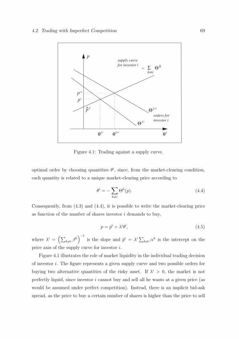
4.2. Trading with Imperfect Competition 69
p
p i
Θi'
− Σ Θh
h=i
^Θ
i''
θi''
supply curve
for investor i
θi
θi'
p''
p'
I
orders for
investor i
Figure 4.1: Trading against a supply curve.
optimal order by choosing quantities θi, since, from the market-clearing condition,
each quantity is related to a unique market-clearing price according to
θi = −∑
h 6=i
Θh(p). (4.4)
Consequently, from (4.3) and (4.4), it is possible to write the market-clearing price
as function of the number of shares investor i demands to buy,
p = pi + λiθi, (4.5)
where λi =(∑
h 6=i βh)−1
is the slope and pi = λi∑
h 6=i αh is the intercept on the
price axis of the supply curve for investor i.
Figure 4.1 illustrates the role of market liquidity in the individual trading decision
of investor i. The figure represents a given supply curve and two possible orders for
buying two alternative quantities of the risky asset. If λi > 0, the market is not
perfectly liquid, since investor i cannot buy and sell all he wants at a given price (as
would be assumed under perfect competition). Instead, there is an implicit bid-ask
spread, as the price to buy a certain number of shares is higher than the price to sell

70 4. Asset Prices under Imperfet Competition
that number of shares. Furthermore, there is price impact, as buying a larger number
of shares drives up the price to buy and selling a larger number of shares drives down
the price to sell. The degree of market liquidity for investor i is determined by the
slope of his supply curve: the steeper the slope, the less liquid the market. The
inverse of the slope, (λi)−1
, is the Kyle (1985, 1989) measure of market depth; we
apply this term to analyze market liquidity.8
The following lemma represents the best-response correspondence for each indi-
vidual investor i.
Lemma 1 Case 1: If βh > 0 for at least one agent h 6= i, then the optimal order for
investor i is given by
Θi,∗(p) =E [v] − ρiVar [v] xi − (1 + r) p
(1 + r)λi + ρiVar [v]. (4.6)
Case 2: If βh = 0 for all h 6= i and∑
h 6=i αh = 0, then investor i is indifferent between
all feasible trading strategies. Case 3: If βh = 0 for all h 6= i and∑
h 6=i αh > 0 (< 0),
then the optimal order for investor i is characterized by αi/βi = +∞ (−∞).
Proof: The problem for investor i is to determine yi and xi to maximize
(1 + r)yi + E [v] xi −ρi
2
(xi)2
Var [v] (4.7)
subject to his budget condition yi + pxi = yi + pxi and the market rules. First,
consider Case 1, where βh > 0 for at least one agent h 6= i. Then, according to (4.5),
there exists a unique market-clearing price p = pi + λi(xi − xi). Plugging the price
into the budget condition yields the trading constraint of investor i as
yi = yi − pi(xi − xi) − λi(xi − xi
)2. (4.8)
Plugging (4.8) into (4.7) for yi and differentiating for xi gives the first-order condition
E [v] − ρixi,∗Var [v] = (1 + r)pi + 2(1 + r)λi(xi,∗ − xi). (4.9)
8Kyle’s (1985) lambda emerges as risk-neutral, price-setting market makers learn private infor-
mation from observing order flow, and Kyle’s (1989) lambda arises as risk-averse investors infer
private information by conditioning their demand schedules on prices in a call auction market. In
our model, illiquidity is not driven by asymmetric information.

4.2. Trading with Imperfect Competition 71
Using the market-clearing price to substitute for pi on the right-hand side of (4.9)
yields the optimal demand to hold shares of the risky asset
xi,∗ (p) =E [v] + (1 + r)λixi − (1 + r) p
(1 + r)λi + ρiVar [v].
The optimal order to buy shares of the risky asset is then given by Θi,∗ (p) = xi,∗ (p)−
xi. For the second-order condition
−2(1 + r)λi − ρiVar [v] < 0
to hold, it is sufficient that βh > 0 for some agent h 6= i. Now, consider the cases
where βh = 0 for all agents h 6= i. Then, investor i does not trade against an
upward-sloping supply curve and, thus, cannot trade different quantities of the risky
asset at different prices. In Case 2, where∑
h 6=i αh = 0, the orders of all other
agents h 6= i aggregate to zero at each price. Consequently, investor i cannot trade
at all and is therefore indifferent between all feasible trading strategies. In Case 3,
where∑
h 6=i αh > 0 (< 0), the aggregate orders of all other agents h 6= i constitute
a (non-zero) market order. Then, investor i obtains maximum expected utility by
submitting a limit order which sells (buys) against this market order and pushes
the price to +∞ (−∞). The Appendix to this chapter spells out the details of
the last two cases, which involve the market rules for situations in which a unique
market-clearing price does not exist. ‖
Figure 4.2 depicts the effect of market liquidity on the individual trading decision
of investor i for Case 1 of Lemma 1. Given the initial endowment at point A, the
curve TC represents the trading constraint (4.8) for λi > 0, and the dashed straight
line is the constraint for the limiting case of a perfectly liquid market as λi → 0
(perfect competition). If λi > 0, investor i acts as a monopsonist over his supply
curve and recognizes that the price moves against him when he trades an additional
unit of the risky asset. As a consequence, his trading aggressiveness is restricted not
only by his risk aversion and the risk of the asset, but also by the level of illiquidity
in the market. The optimal order equates marginal expected utility of the risky
asset with marginal costs, including liquidity costs (point B). The figure shows that
liquidity costs from imperfect competition reduce trading volume and expected utility
for investor i compared to the optimum in the perfectly competitive case (point C).

72 4. Asset Prices under Imperfet Competition
yi
xix i
xi'
θi'
xi,c
A
B
C
TC
yi
indifference curves
of investor i
trading constraint
for investor i
Figure 4.2: Market liquidity in the individual trading decision.
Case 1 of Lemma 1 provides the equilibrium discussed in the next sections. In this
equilibrium, each investor submits a limit order and trade takes place; we refer to this
equilibrium as trading equilibrium. In addition to the trading equilibrium, there exists
also an equilibrium in which each investor employs the passive investment strategy.
The remainder of this section argues that this equilibrium in passive strategies is of
minor interest in our model.
Proposition 1 There exists an equilibrium in which each investor plays the passive
strategy. For each investor i, the passive strategy is weakly dominated by any limit
order of the form
αi = ki
(E [v]
ρiVar [v]− xi
1
)
, βi = ki (1 + r)
ρiVar [v]with 1 ≥ ki > 0. (4.10)
Proof: See Appendix to this chapter. ‖
The existence of the equilibrium in passive strategies is straightforward to under-
stand: if no agent h 6= i submits any order, then not-submitting an order is an optimal

4.3. Equilibrium with Identical Risk Aversion 73
response for investor i, and vice versa. This trivial equilibrium with each agent doing
nothing is a standard result in fully strategic trading games. As the passive strategy,
however, is weakly dominated by any limit order (4.10), the trivial equilibrium is not
a compelling prediction of our model (even though the choice of a weakly dominated
strategy cannot be ruled out with arguments of rationality alone—in contrast to a
strictly dominated strategy).
A formal way to rule out the equilibrium in passive strategies is to introduce
exogenous noise traders who submit a random aggregate order z ∼ N (0, σ2z), thereby
provide a (non-zero) market order with probability one, and thus attract limit orders
from all optimizing investors. Intuitively, when there are noise traders who have
“trembling hands” in their order decisions, other investors become willing to place
limit orders in the market to make profits by trading against the random market
orders. However, since noise traders have no further role in our symmetric information
model, we do not carry out this refinement formally.
4.3 Equilibrium with Identical Risk Aversion
In this section, we study a trading equilibrium, in which each investor submits a limit
order and trade takes place. First, we establish the existence of a unique trading equi-
librium. Then, we analyze the determinants of market liquidity and how illiquidity
affects the market-clearing price and the allocation of the risky asset. We restrict the
analysis in this section to the case that all investors have identical risk aversion and
submit limit orders with identical slope, i.e., we assume ρi = ρ for all i and βi = β
for all i. This case is analytically very tractable and provides much of the intuition
for our asset pricing model with imperfect competition.
The following proposition represents the trading equilibrium for the case of iden-
tical risk aversion for all investors.
Proposition 2 Consider the case of linear orders, and assume ρi = ρ for all i and
βi = β for all i. If I ≥ 3, then there exists a unique trading equilibrium given by
αi,∗ =(I − 2)
(I − 1)
(E [v]
ρVar [v]− xi
)
, βi,∗ =(I − 2)
(I − 1)
(1 + r)
ρVar [v]for all i. (4.11)
If I = 2, then a trading equilibrium does not exist.

74 4. Asset Prices under Imperfet Competition
Proof: The trading equilibrium follows from Case 1 of Lemma 1, in which for each
investor i, βh > 0 for at least one agent h 6= i. The equilibrium is derived by equating
the parameters from the conjectured order (4.2) with those from the optimal order
in the best response (4.6) for each investor i, i.e., the equilibrium is the solution to
the following equation system
αi,∗ =E [v] − ρiVar [v] xi
(1 + r)(∑
h 6=i βh,∗
)−1
+ ρiVar [v]i = 1, . . . , I, (4.12)
βi,∗ =(1 + r)
(1 + r)(∑
h 6=i βh,∗
)−1
+ ρiVar [v]i = 1, . . . , I. (4.13)
Using the symmetry assumptions on ρi and βi, (4.13) can be solved immediately.
Plugging the solution for β into (4.12) yields the solution for αi for each investor i.
The second solution to (4.13), β = 0, does not yield an equilibrium from Case 1,
as it violates the condition that for each investor i, βh > 0 for at least one agent
h 6= i. The other cases in Lemma 1 do not yield additional trading equilibria (only
the passive equilibrium from Case 2). If I = 2, there is no relevant solution to
(4.13) and, thus, a trading equilibrium does not exist—even without the symmetry
restrictions on ρi and βi. ‖
In the trading equilibrium (4.11), each investor submits a limit order, a unique
market-clearing price exists, and there is trade. The structure of the equilibrium
orders under imperfect competition is similar to the orders under perfect competition.
The only difference under imperfect competition is that each investor restricts the
aggressiveness of his limit order by the coefficient k := (I − 2)/(I − 1) < 1, whereas
the coefficient is equal to one when investors act under the assumption of perfect
competition.
The assumption of identical βi for all i (in addition to the assumption of identical
ρi for all i) is used to prove that there does not exist another trading equilibrium.
We conjecture that uniqueness of the trading equilibrium holds also without this
assumption, but do not attempt to prove this here. A trading equilibrium does not
exist, when there are only two investors. In this case, no investor is willing to submit
any order, because the order would be exposed to the total market power of the other
agent. The presence of a third agent, however, generates the necessary competition

4.3. Equilibrium with Identical Risk Aversion 75
to make each investor willing to become active in the market and for the trading
equilibrium to exist.
Now, we turn to the properties of the trading equilibrium. First, we relate an
investor’s price impact from imperfect competition to the notion of market liquidity
as it is prevalent in market microstructure theory.
Proposition 3 For each investor i, the degree of market liquidity is given by
λ−1 =(1 + r)(I − 2)ρ−1
Var [v]. (4.14)
Proof: The result follows immediately from the definition of λi and the solution to
βi. Because of the assumptions of identical ρi and βi for all i, market liquidity is
identical for all investors, too. ‖
The rationale of this result is straightforward. If, for instance, investor i wishes
to sell shares of the risky asset, he has to make other agents willing to buy these
shares for the market to clear. Since the orders of the other agents are decreasing
in price, the market is not perfectly liquid and investor i moves the price downward
when selling his shares. The price impact (per share) is the smaller, and accordingly
the degree of market liquidity is the higher, the larger the number of other agents
and their risk tolerance and the smaller the risk of the asset.
The result on market liquidity corresponds qualitatively to the inventory-based
microstructure approaches of Stoll (1978), Ho and Stoll (1981, 1983), and Gross-
man and Miller (1988). In these microstructure models, risk-averse market makers
provide trading immediacy by accomodating orders from other market participants,
and illiquidity (in terms of bid-ask spreads or price concessions) arises to compensate
market makers for their willingness to change the risk profile of their inventory. In
our model, market liquidity is not determined by the activity of a market maker,
but is provided by the mutual submission of limit orders from investors themselves.
Since these orders, however, reflect investors’ portfolio decisions, our model captures
the risk-aversion based aspect of market liquidity from the microstructure literature
nevertheless.
Next, we turn to the market-clearing price and investors’ portfolio holdings of the
risky asset and study how these variables are affected by illiquidity. In particular, we

76 4. Asset Prices under Imperfet Competition
are interested in whether the expected return of the risky asset reflects, beyond the
standard risk premium, an additional liquidity premium that confirms the notion of
compensation required by investors for their liquidity costs.
Proposition 4 The market-clearing price and investors’ portfolio holdings of the
risky asset are given by
p =1
(1 + r)
(
E [v] −XVar [v]
Iρ−1
)
(4.15)
and
xi = xi +(I − 2)
(I − 1)
(X
I− xi
)
for all i.
Proof: The market-clearing price follows from the market-clearing condition (4.1),
the equilibrium orders (4.11), and from∑I
i=1xi ≡ X. The number of shares bought
or sold by investor i are determined by plugging the market-clearing price into the
equilibrium order of the investor. Portfolio holdings are then given by xi = xi + θi. ‖
For the case of identical risk aversion for all investors, the market-clearing price
under imperfect competition is equal to the corresponding price under perfect compe-
tition: it is given by the expected payoff per share minus the standard risk premium,
both discounted at the riskfree rate of interest. In particular, the market-clearing
price under imperfect competition does not reflect an additional liquidity discount,
and equivalently the expected return does not yield an additional liquidity premium.
The allocation of the risky asset, however, is in general different from the Pareto-
optimal, risk-tolerance-weighted allocation under perfect competition, which simpli-
fies to xc = X/I for all i in the case of identical risk aversion. Under imperfect com-
petition, investors trade towards the Pareto-optimal allocation, but do not achieve
this allocation completely. If, for instance, investor i is endowed with only few shares
of the risky asset, xi < xc, he buys additional shares at the market-clearing price and
obtains the portfolio holdings xi with xi < xi < xc. Trading volume for an individual
investor i is given by
θi =(I − 2)
(I − 1)
(xc − xi
)=
(I − 2)
(I − 1)θi,c,

4.3. Equilibrium with Identical Risk Aversion 77
θ1'
demand to buyp
θi
supply to sell
p'
θ1,c
Θ1,*
Θ2,*
θ2'θ
2,c
Θ1,cΘ
2,c
Figure 4.3: Pricing effect of illiquidity with endogenous trading.
and aggregate trading volume in the economy is given by
V =1
2
I∑
i=1
∣∣ θi∣∣ =
(I − 2)
(I − 1)V c.
Consequently, liquidity costs from imperfect competition in general reduce trading
volume and impede optimal risk sharing among investors. Only for the special case
that each investor’s initial endowment already corresponds to his holdings under
optimal risk sharing (i.e. xi = xc for all i), illiquidity does not impair trading volume
and optimal risk sharing. In this case, however, there is obviously no potential for
mutually beneficial trade in the first place (although investors submit their limit
orders nonetheless).
Figure 4.3 illustrates the results on the market-clearing price and on trading vol-
ume for an example with I = 3, x1 < xc < x2, and x3 = xc. In this example, trade
takes place only between i = 1 and i = 2, but the presence of i = 3 is needed for
the trading equilibrium with imperfect competition to exist. Investors’ orders under
imperfect competition can, from (4.11), be written
p =E [v] − ρVar [v] xi
(1 + r)− k−1 ρVar [v]
(1 + r)θi, (4.16)

78 4. Asset Prices under Imperfet Competition
with k−1 = (I − 1)/(I − 2), and are represented by the solid lines in the figure.9
It can be seen that the market clears at price p′ and trades are given by θ1′ =
−θ2′. In comparison, investors’ orders under perfect competition are similar to (4.16),
except that the assumption of price-taking behavior implies that kc = 1. Thus,
each investor’s order intersects the price axis at the same point as his order under
imperfect competition, but is less steeply sloped, as shown by the dashed lines in the
figure. Consequently, if investors act as if there are no liquidity costs from imperfect
competition, the market clears at the same price p′, but investors i = 1, 2 trade a
higher volume θ1,c = −θ2,c.
The result on the market-clearing price is the main point of this chapter—it
stands in contrast to the literature on exogenous trading costs in the line of Amihud
and Mendelson (1986) and others, which finds that illiquidity reduces the price of
an asset and, equivalently, increases the expected return of an asset, as investors
require compensation for bearing liquidity costs. In our model, illiquidity is a cost,
but it is not a priced factor. The reason is that buyers respond to liquidity costs
by reducing their demand to buy and sellers by reducing their supply to sell, and
these individual effects cancel each other with respect to the market-clearing price.
Intuitively, as can be seen from Figure 4.3, buyers (i = 1) demand a price discount,
and sellers (i = 2) demand a price premium, and thus both sides of the market would
like to be compensated for their liquidity costs, but nobody is willing to grant that
compensation. In the next section, we analyze this cancelling out in more detail for
the case that investors have heterogeneous risk aversion.
Investors’ trading decisions under imperfect competition reveal further microstruc-
ture features of market liquidity. If investor i, for instance, increases his order ag-
gressiveness (in the sense of trading more price-elastically by choosing a higher ki),
he adversly affects his trading price, but he also generates a positive externality by
improving liquidity for all other agents h 6= i.10 Other agents are then willing to
9The order for investor i = 3, which is parallel to Θ1,∗ and Θ2,∗ and intersects the price axis at
the market-clearing price, is omitted in the figure.10The empirical microstructure literature on limit order books distinguishes between two concepts
of order aggressiveness (say for buy orders): (i) trade aggressiveness, where the most aggressive order
type is a large buy order that results in immediate execution and walks up the book above the best
ask price (e.g. Biais, Hillion, and Spatt (1995)); and (ii) limit order aggressiveness, where the most
aggressive type is a limit buy order that specifies a limit price above the best existing bid price
4.3. Equilibrium with Identical Risk Aversion 79
trade more aggressively themselves and thereby improve market liquidity for investor
i, too. Thus, liquidity provision of each individual investor to the rest of the market
is associated with a positive feedback effect of improved liquidity for that investor
himself. This mutually re-inforcing liquidity provision among investors illustrates
the strategic complementarity property of market liquidity and is captured in the
common phrase that “liquidity begets liquidity.”
In equilibrium, the price impact effect and the positive feedback effect are bal-
anced, and no investor has an incentive to trade more aggressively, as his adverse price
effect would not be offset by additional liquidity provision to him. Put differently, the
submission of perfect competition orders by all investors to mutually enhance market
liquidity (and trade the Pareto-optimal quantity at the same price as under imper-
fect competition) is not an equilibrium, since each investor would have an incentive
to deviate by restricting his order aggressiveness to obtain a more favorable price.11
Consequently, if market liquidity is endogenous, then the positive externality of liq-
uidity provision leads to an insufficient level of liquidity in the market and thereby
obstructs the processing of the Pareto-optimal trading volume.
We conclude this section with a competitive limit analysis of the imperfectly
competitive trading equilibrium. It is a well acknowledged result in the economics
literature that the assumption of perfect competition is problematic for markets with
a finite number of participants, because price-taking behavior requires each agent to
ignore the strategic influence he de facto has (Roberts and Postlewaite (1976)). Yet,
the price-taking assumption is commonly motivated as a plausible approximation for
trading behavior and market outcomes when there is a large number of agents in the
market and each agent is small relative to the rest of the market.12 The following
proposition examines this large market justification of price-taking behavior in the
context of asset pricing theory.
and is stored in the book (Harris and Hasbrouck (1996)). The notion of aggressiveness in our call
auction market corresponds to the second concept.11This can be seen analytically from an out-of-equilibrium study in the example underlying Fig-
ure 4.3. Assume, investors i = 1, 3 submit perfect competition orders, i.e. orders (4.16) with
k1 = k3 = 1. Then the optimal response for investor i = 2 is (from (4.6)) to submit an order (4.16)
with k2 = 2/3 < 1 so as to obtain a higher price p′′ > p′ for his sale. (Perfect competition orders
are not optimal for i = 1, 3 then either.)12For further references and a short summary of the arguments on price-taking behavior, see the
introduction in Hellwig (2005).

80 4. Asset Prices under Imperfet Competition
Proposition 5 If the number of investors goes to infinity, then the market becomes
perfectly liquid, equilibrium orders converge to perfect competition orders, and the
expected return of the risky asset decreases to the riskfree rate of interest.
Proof: The results follow immediately from taking the limits in (4.11), (4.14), and
(4.15) for I → ∞. ‖
The results on market liquidity and equilibrium orders are in line with the common
justification of price-taking behavior as an approximation for large markets: if the
number of investors is large, then each investor faces a flat supply curve and thus
can trade different quantities of shares at a given price. At the same time, however,
the expected return of the risky asset reduces to the riskfree rate and, equivalently,
the risk premium goes to zero. Although this concurrent vanishing of price impact
and risk premium in our model is driven by the “risk elimination” property of CARA
investors (Lintner (1970)), the intuition applies more generally: for each investor to
be small relative to the rest of the market and to have zero price impact, the market
must be so large that the price of risk is zero as well.
Consequently, our analysis of strategic trading interactions casts an ambiguous
light on the assumption of price-taking behavior in asset pricing theory. On the one
hand, the competitive limit results show that under conditions that justify price-
taking behavior the analysis of risk-return relations becomes pointless, since the
market, in aggregate, must be risk neutral. On the other hand, the result on the
market-clearing price suggests that prices may be similar to those predicted under
the assumption of price-taking behavior, even if investors have (and recognize) price
impact, i.e., even if the market is small.
4.4 Heterogeneity in Risk Aversion
In this section, we study the trading equilibrium for the case that investors have
heterogeneous risk aversion. The structure of the analysis is similar to the case of
identical risk aversion, but the model becomes much less tractable. We thus restrict
the model to the simplest possible case of heterogeneity with only three investors
and two different degrees of risk aversion, i.e., we assume I = 3 and ρ1 6= ρ2 =

4.4. Heterogeneity in Risk Aversion 81
ρ3. Variables that are identical for investors i = 2, 3 are sometimes indicated by a
superscript n instead of the general index i (e.g. we often use ρn := ρ2 = ρ3).
The following proposition establishes the trading equilibrium for the case of het-
erogeneity in investors’ risk aversion.
Proposition 6 Consider the case of linear orders, and assume I = 3, ρn := ρ2 = ρ3,
and βn := β2 = β3. Then there exists a unique trading equilibrium given by
α1,∗ = k1
(E [v]
ρ1Var [v]− x1
)
, β1,∗ = k1 (1 + r)
ρ1Var [v], (4.17)
αi,∗ = kn
(E [v]
ρnVar [v]− xi
)
, βi,∗ = kn (1 + r)
ρnVar [v], i = 2, 3, (4.18)
with
k1 ≡
√
ρn (16ρ1 + 9ρn) − 3ρn
√
ρn (16ρ1 + 9ρn) − ρn< 1, (4.19)
kn ≡4ρn
√
ρn (16ρ1 + 9ρn) + 3ρn< 1. (4.20)
Heterogeneity in risk aversion affects the coefficients of order aggressiveness, ki, ac-
cording to
ρ1
>
=
<
ρn ⇒ k1
>
=
<
kn. (4.21)
Proof: See Appendix to this chapter. ‖
In the trading equilibrium with heterogeneous risk aversion, each investor’s order
is again given by his perfect competition order multiplied by a coefficient ki < 1,
which restricts the aggressiveness of the limit order. However, the coefficients of
order aggressiveness are now different for investors with different risk aversion: an
investor with higher risk aversion has a higher coefficient ki, i.e., a more risk-averse
investor restricts his order less strongly than a less risk-averse agent (compared to
the corresponding order under perfect competition).
Now, we turn to the properties of the trading equilibrium with heterogeneous risk
aversion. First, we analyze market liquidity.

82 4. Asset Prices under Imperfet Competition
Proposition 7 Market liquidity for the different investors is given by
(λ1)−1
=8(1 + r)
[√
ρn (16ρ1 + 9ρn) + 3ρn
]
Var [v](4.22)
and
(λi)−1
=4(1 + r)
[√
ρn (16ρ1 + 9ρn) − ρn
]
Var [v], i = 2, 3. (4.23)
Proof: See Appendix to this chapter. ‖
Market liquidity for each investor is again determined by the risk-bearing willing-
ness of the other agents in the market and, hence, is decreasing in the risk aversion
of the other agents and in the risk of the asset. Heterogeneity in risk aversion reveals
additional aspects of the strategic interdependency in the model, however. First,
market liquidity for an investor can be related to his own risk aversion. From (4.22)
it can be seen for investor i = 1 that
∂(λ1)−1
∂ρ1< 0,
i.e., market liquidity for the investor is decreasing in his own risk aversion. This
comparative static result reflects the feedback effect of liquidity provision: when
the risk aversion of an investor increases, he reduces his liquidity provision to other
agents by trading less aggressively and, because of strategic complementarity in order
aggressiveness, experiences a decline in liquidity provision by other agents to himself
in return.13
Second, heterogeneity in risk aversion leads to cross-sectional differences in market
liquidity. A comparison of (4.22) and (4.23) shows that
ρ1
>
=
<
ρn ⇒ (λ1)−1
>
=
<
(λn)−1,
i.e., the market is more liquid for investors with higher risk aversion. Put differently,
an investor is “large” in terms of his price impact (per share), if he has a large
13For investors i = 2, 3 the effect cannot be shown analytically, since a change in ρn cannot be
related uniquely to either of the two.

4.4. Heterogeneity in Risk Aversion 83
risk tolerance compared to other agents in the market. The cross-sectional result is
in line with the intuitive notion that large investors are characterized by high risk-
bearing capacity and that large investors are major providers of market liquidity by
submitting aggressive limit orders, but face illiquid markets for their own trading
needs.
Next, we consider how differences in market liquidity among investors affects the
market-clearing price of the risky asset.
Proposition 8 The market-clearing price of the risky asset is given by
p =1
(1 + r)
(
E [v] −XVar [v]
1/ρ1 + 2/ρn
)
− Z,
where
Z ≡3∑
i=1
1/ρi
1/ρ1 + 2/ρnλi(xi − xi
). (4.24)
Proof: See Appendix to this chapter. ‖
For the case of heterogeneous risk aversion, the market-clearing price under im-
perfect competition is equal to the corresponding price under perfect competition
minus an additional term Z. Thus, illiquidity from imperfect competition has a pric-
ing effect in general. The additional pricing term Z has a nice interpretation relating
to the idea that investors require compensation for bearing liquidity costs. Equation
(4.24) reveals that each investor i demands a risk-tolerance-weighted price concession
for his liquidity costs, which is given by his price impact per share, λi, times his
trading volume, xi − xi. Consequently, the pricing effect of illiquidity Z can indeed
be traced back to the notion of compensation for liquidity costs on the individual
investor level.
On the aggregate level, however, the individual effects again counterbalance each
other, as the required price concessions are a price discount for buyers and a price
premium for sellers.14 In particular, it can be seen from (4.24) that the cancelling out
of individual effects is exact and hence the perfect competition price arises (Z = 0),
14Note that, say, the price discount required by a buyer is his required price concession relative
to the perfect competition price. For the overall price, in contrast, a buyer bids the price up, not
down.

84 4. Asset Prices under Imperfet Competition
if there are no trades between investors with different risk aversion.15 This condition
includes, but is not limited to, two special cases: (i) all investors have identical risk
aversion—then the perfect competition price arises independently of investors’ initial
endowments and the corresponding trades (as already shown in the previous section);
and (ii) each investor’s initial endowment corresponds to his holdings under optimal
risk sharing—then the perfect competition price arises independently of investors’
risk aversion as there is no basis for trade in the first place.
If, in contrast, the cancelling out between the individually required price conces-
sions is not exact, then using the symmetry assumptions for investors i = 2, 3 to
rewrite (4.24) as
Z =1
1/ρ1 + 2/ρn
[(λ1
ρ1−λn
ρn
)(x1 − x1
)]
shows that the price is distorted towards the side of the market on which the larger
investor (characterized by high risk tolerance and price impact) is trading. That
is, the pricing effect of illiquidity is a discount compared to the price under perfect
competition (Z > 0), if the larger investor is a buyer, and the pricing effect is a
premium (Z < 0), if the larger investor is a seller.16 Intuitively, the larger investor
requires a higher price concession for his liquidity costs and, thus, dominates the
aggregate effect on the price.
In summary, the pricing effect of illiquidity Z is different from the standard liq-
uidity premium derived in asset pricing models on exogenous trading costs, which
find that illiquidity is priced as an additional premium on the expected return of
an asset and that the liquidity premium, in turn, is increasing in investors’ liquidity
costs. In our model, in contrast, the effects of investors’ liquidity costs on the price
and on the expected return “net out” to a greater or lesser extent, and the aggregate
pricing effect of illiquidity is merely a residual term or price distortion, which can be
positive or negative and which is not directly related to the degree of illiquidity in
the market.
15In our economy with only two different degrees of risk aversion, this condition is also necessary.
We conjecture that the necessity part of the condition does not hold with more heterogeneity in risk
aversion.16Since trades between agents with identical risk aversion offset exactly with respect to the price,
for investors i = 2, 3 the aggregate trade (x2−x2)+(x3−x3) ≡ −(x1−x1) is relevant for determining
their side of the market.

4.4. Heterogeneity in Risk Aversion 85
Finally, we study the effects of heterogeneity in risk aversion on investors’ portfolio
holdings of the risky asset.
Proposition 9 Investors’ portfolio holdings of the risky asset are given by
x1 = x1 + φ(x1,c − x1
), (4.25)
xi = xi + φ(xn,c − xi
)+ ξ
(xi − xh
)i, h = 2, 3, i 6= h, (4.26)
where
φ ≡k1kn (2ρ1 + ρn)
2knρ1 + k1ρn< 1 and ξ ≡
(k1 − kn) knρ1
2knρ1 + k1ρn. (4.27)
Proof: See Appendix to this chapter. ‖
The allocation of the risky asset is again governed by the improvement of risk
sharing under imperfect market liquidity. If the initial endowment of investor i de-
viates from his holdings under optimal risk sharing, then the trade of the investor
has a standard risk sharing effect φ (xi,c − xi), adjusting the portfolio holdings to-
wards optimal risk sharing but only incompletely because of illiquidity (φ < 1). The
trades of investors i = 2, 3, however, exhibit an additional “heterogeneity effect”
ξ(xi − xh
). The heterogeneity effect either re-inforces or countervails the risk shar-
ing effect, depending on the relation between the risk aversions ρ1 and ρn (which from
(4.21) and (4.27) determines the sign of ξ) and depending on the relation between
the endowments x2 and x3.
To illustrate the interplay between the risk sharing effect and the heterogeneity
effect, we consider an example with x1 < x1,c and x2 = xn,c < x3. In this example, the
initial endowment of investor 2 already corresponds to his holdings under optimal risk
sharing, and the trade to establish the Pareto-optimal allocation of the risky asset
reduces to x1,c − x1 = − (xn,c − x3) > 0 between investor 1 and investor 3. Under
perfect competition, this Pareto-optimal trade between i = 1 and i = 3 takes place,
and trading volume in the economy is thus given by V c = (x1,c − x1). Under imperfect
competition, in contrast, investor 2 also trades a non-zero number of shares due to
the heterogeneity effect and thereby trades away from his holdings under optimal risk

86 4. Asset Prices under Imperfet Competition
xi
θ1
Case 1: ρ1< ρn
x1,cx1x1xn,c= x2 x2 x3 x3
θ2
θ3
φ3
ξ3
Case 2: ρ1 > ρn
xix1 x2x1,c x3xn,c= x2 x3x1
φ3
ξ3
θ3
θ2
θ1
Figure 4.4: Trading volume with heterogeneity effect.
sharing. Using x2 = xn,c, investors’ portfolio holdings in the example follow as
x1 = x1 + φ(x1,c − x1
)< x1,c,
x2 = xn,c + ξ(xn,c − x3
),
x3 = x3 + (φ− ξ)(xn,c − x3
)> xn,c,
with
φ− ξ =(k1 + kn) knρ1 + knk1ρn
2knρ1 + k1ρn< 1.
Whether investor 2 acts as buyer (x2 > xn,c) or as seller (x2 < xn,c) depends on the
relation between ρ1 and ρn and, hence, on who is the larger investor in the economy.
In the following, we examine the two possible cases of heterogeneity for the example
in detail; a graphical illustration is given in Figure 4.4.
Case 1: First, consider the case that ρ1 < ρn (⇒ ξ < 0), so that investor 1
is the larger investor in the economy. As i = 1 acts as buyer in the example, the
pricing effect of illiquidity is a discount relative to the price under perfect competition
(Z > 0). Because of the price discount, in turn, investor 2 is willing to buy shares of
the risky asset via the heterogeneity effect (ξ (x2 − x3) > 0) and obtains the portfolio
holdings x2 > xn,c. Conversely, investor 3 sells shares by the heterogeneity effect

4.4. Heterogeneity in Risk Aversion 87
(ξ (x3 − x2) < 0) and thereby re-inforces his selling from the risk sharing effect. Yet,
despite the re-inforcing trading from the heterogeneity effect, the portfolio of i = 3 is
still distorted towards his initial endowment (φ−ξ < 1). Similarly, aggregate trading
volume in the economy,
V = (φ− ξ)(x1,c − x1
)= (φ− ξ)V c,
is increased by the heterogeneity effect beyond the trading from the risk sharing effect
(ξ < 0), but is still lower than under perfect competition.
Case 2: Now, consider the case that ρ1 > ρn (⇒ ξ > 0), so that investor 3
is the larger investor in the economy. As i = 3 acts as seller, illiquidity generates
a premium on the price (Z < 0). At this higher price, investor 2 is willing to
sell shares via the heterogeneity effect (ξ (x2 − x3) < 0) and obtains the portfolio
holdings x2 < xn,c. Conversely, investor 3 buys shares from the heterogeneity effect
(ξ (x3 − x2) > 0), which coutervails his selling from the risk sharing effect. Hence,
the trade of i = 3 towards his portfolio under optimal risk sharing is partly crowded
out by the heterogeneity effect. Likewise, aggregate trading volume in the economy,
V = φ(x1,c − x1
)= φV c,
is not increased beyond the trading from the risk sharing effect.
Figure 4.4 depicts the individual trading volumes for the two cases of the exam-
ple. For each case, trading volume of investor 3 is composed of a risk sharing part,
indicated by φ3 := φ (xn,c − x3), and a heterogeneity part, ξ3 := ξ (x3 − x2). Note
that in both cases of the example, investor 2 trades via the heterogeneity effect on
the same side of the market as the larger investor in the economy. That is, investor 2
does not step in as a counterparty in order to alleviate the price impact of the large
investor’s risk-sharing trade, but instead trades in the same direction and thereby
even re-inforces the large investor’s price impact. Consequently, if an investor trades
exclusively because of the heterogeneity effect, his activity is reminiscent of market
manipulation against the trading need of a large investor in an illiquid market.17
17However, models on market manipulation against large investors are usually based on asym-
metric information or exogenous endowment shocks (see, e.g., Vayanos (2001), Brunnermeier and
Pedersen (2005), and Pritsker (2005)), which is not the case in our model.

88 4. Asset Prices under Imperfet Competition
4.5 Discussion
In this chapter, we study a static asset pricing model with imperfect competition
and endogenous market liquidity. We find that liquidity costs reduce trading volume
and impede Pareto-optimal risk sharing among investors. The expected return of
the risky asset, however, is not systematically affected by liquidity costs and, thus,
reflects only a risk premium but no liquidity premium—contrary to the prediction of
liquidity premia in the literature on exogenous trading costs cited in the introduction
to this chapter. This result deserves further discussion.
A possible objection to the absence of a liquidity premium in our model is that
market liquidity, although it exhibits several typical microstructure properties, is
captured incompletely. First, illiquidity originates from investors’ risk-bearing costs
only. Other microstructure frictions, e.g. asymmetric information or search costs, are
not considered. Next, our model of one-shot trading precludes any effects of future
liquidity costs on current asset prices, for instance as in a dynamic model in which
investors trade repeatedly over time to further improve risk sharing or because of
exogenous wealth shocks. Finally, liquidity costs are not stochastic. Even though
under simultaneous order submission, an investor cannot observe his supply curve
before making his own trading decision, the common knowledge assumption of the
model allows each investor to infer the degree of market liquidity in equilibrium with
certainty. The argument that our setting captures only a part of the multi-faceted
concept of market liquidity is thus well justified. However, this argument is not
crucial for the absence of a liquidity premium.
The crucial point for the absence of a liquidity premium is the endogeneity of
trading on both sides of the market. It is for this reason that the price discount
required as compensation for liquidity costs by buyers is offset by a price premium
required by sellers. In particular, if sellers were instead exogenously forced to liquidate
their portfolios, then their offsetting effect on the price would be eliminated and,
consequently, a liquidity premium on the expected return would arise in our model.
A closely related result is found by Vayanos (1998) in a competitive overlapping
generations model with exogenous bid-ask spreads and endogenous trading horizons.
In his model, an increase in liquidity costs has two opposing effects, either of which

Appendix: Proofs to Chapter 4 89
can dominate asset prices: on the one hand, new investors are less willing to buy the
illiquid asset, but on the other hand, older investors sell back their asset holdings
more slowly. Vayanos (1998) shows that the second effect always offsets the standard
liquidity premium to some extent. Moreover, when the second effect dominates, then
asset prices are actually increasing in liquidity costs.
In conclusion, the absence of a liquidity premium in the model presented in this
chapter is not primarily driven by an incomplete view of market liquidity, but rather
by the endogeneity of trading on both sides of the market. However, it is nevertheless
promising to consider the asset pricing implications of illiquidity in a richer setting
allowing for both dynamic and stochastic trading effects. These issues are addressed
in the next chapter.
Appendix: Proofs to Chapter 4
Proof of Lemma 1 (Continuation)
Here, we consider in more detail the last two cases of Lemma 1, where investor i
trades against a vertical supply curve, which offers the same quantity of shares at
each possible price.
In Case 2, the supply curve for investor i is given by βh = 0 for all h 6= i and∑
h 6=i αh = 0. If i submits a limit order 〈αi, βi > 0〉, then there exists a unique market-
clearing price p′ = αi/βi. At this price, Θi(p′) = 0 applies, i.e., trading volume for i is
zero. (There is trade between other agents, however, if αh 6= 0 for at least two h 6= i.)
If i submits a market order 〈αi 6= 0, βi = 0〉, then there does not exist a market-
clearing price, and if i employs the passive strategy 〈αi = 0, βi = 0〉, then every price
clears the market. Since the market rules exclude trade when there does not exist
a unique market-clearing price, trading volume for i again is zero. Consequently, in
Case 2, investor i does not trade, but remains with his initial endowments for each
possible order choice. Thus, investor i is indifferent between all of his feasible trading
strategies.
In Case 3, the supply curve for investor i is given by βh = 0 for all h 6= i and∑
h 6=i αh > 0 (< 0). If i submits a market order 〈αi 6= 0, βi = 0〉 or employs the
passive strategy 〈αi = 0, βi = 0〉, then either no price clears the market (if αi 6=

90 4. Asset Prices under Imperfet Competition
−∑
h 6=i αh), or every price clears the market (if αi = −
∑
h 6=i αh); in both cases, no
trade takes place, and i remains with his initial endowments. If i submits a limit
order 〈αi, βi > 0〉, then there exists a unique market-clearing price, and i sells (buys)∣∣∣∑
h 6=i αh
∣∣∣ shares. For trading against a vertical supply curve, investor i can force the
price for a sale (purchase) to +∞ (−∞) by setting αi/βi = ∞ (−∞), which gives
higher expected utility than holding his initial endowment. Since the corresponding
trade would not be optimal for at least one other agent h 6= i, however, Case 3
does obviously not yield an equilibrium. Therefore, we skip the exact specification
of the best response for this case, which is a purely technical problem of imposing
restrictions on the parameters αi and βi. ‖
Proof of Proposition 1
The equilibrium in passive strategies follows from Case 2 of Lemma 1. In this case we
have, for each investor i, βh = 0 for all h 6= i and∑
h 6=i αh = 0. Then, each investor
i is indifferent between all feasible trading strategies, including the passive strategy.
This gives the equilibrium.
To prove the weak domination part of the proposition, we have to show that for
investor i, any limit order
αi = ki
(E [v]
ρiVar [v]− xi
1
)
, βi = ki (1 + r)
ρiVar [v]with 1 ≥ ki > 0 (4.28)
does at least as well as passive investment for all feasible trading strategies of the
other agents h 6= i and does strictly better than passive investment for some strategies
of other agents. First, substitute the budget constraint into the payoff function to
write the objective function of investor i as
(1 + r)[yi − p(xi − xi)
]+ E [v] xi −
ρi
2
(xi)2
Var [v] . (4.29)
If i employs the passive investment strategy, then he does not trade and his expected
utility is determined by
(1 + r)yi + E [v] xi −ρi
2
(xi)2
Var [v] , (4.30)
irrespective of the strategies chosen by all other agents h 6= i. If i submits a limit

Appendix: Proofs to Chapter 4 91
order (4.28), then a unique market-clearing price
p′ =kiE [v] + ρiVar [v]
(∑
h 6=i αh − kixi
)
ki(1 + r) + ρiVar [v]∑
h 6=i βh
(4.31)
exists, and, by plugging (4.31) into the order specified by (4.28), trading volume of i
is given by
θi′ =ki[
(E [v] − ρiVar [v] xi)∑
h 6=i βh − (1 + r)
∑
h 6=i αh]
ki(1 + r) + ρiVar [v]∑
h 6=i βh
. (4.32)
Next, comparing (4.29) with (4.30) shows that a limit order weakly dominates the
passive investment strategy for investor i, if the condition
θi
[
E [v] − (1 + r)p−ρi
2
(θi + 2xi
)Var [v]
]
≥ 0 (4.33)
holds for all feasible trading strategies of all other agents h 6= i and holds with strict
inequality for some strategies of other agents. Finally, plugging (4.31) and (4.32) into
(4.33) and simplifying yields
(2 − ki)kiρiVar [v][
(E [v] − ρiVar [v] xi)∑
h 6=i βh − (1 + r)
∑
h 6=i αh]2
2[
ki(1 + r) + ρiVar [v]∑
h 6=i βh
]2 ≥ 0,
which, under the sufficient restriction 1 ≥ ki > 0, completes the proof. ‖
Proof of Proposition 6
The trading equilibrium follows again from Case 1 of Lemma 1. Using the assump-
tions on the number of investors and on heterogeneity in risk aversion, the equilibrium
is the solution to the equation system
α1,∗ =E [v] − ρ1Var [v] x1
(1 + r)/ (2βn,∗) + ρ1Var [v], (4.34)
β1,∗ =(1 + r)
(1 + r)/ (2βn,∗) + ρ1Var [v], (4.35)
αi,∗ =E [v] − ρnVar [v] xi
(1 + r)/ (β1,∗ + βn,∗) + ρnVar [v]i = 2, 3, (4.36)
βn,∗ =(1 + r)
(1 + r)/ (β1,∗ + βn,∗) + ρnVar [v]. (4.37)

92 4. Asset Prices under Imperfet Competition
First, rearranging (4.37) yields
βn,∗(β1,∗ + βn,∗
)ρnVar [v] − β1,∗(1 + r) = 0. (4.38)
Then, writing (4.35) as
β1,∗ =2βn,∗(1 + r)
(1 + r) + 2βn,∗ρ1Var [v](4.39)
and using (4.39) to eliminate β1,∗ from (4.38) gives
βn,∗[(βn,∗)2 2ρ1ρn (Var [v])2 + βn,∗3(1 + r)ρnVar [v] − 2 (1 + r)2
]= 0. (4.40)
The relevant solution to (4.40), which does not violate the trading rules and the
conditions in Case 1 of Lemma 1, is given by
βn,∗ = −3(1 + r)
4ρ1Var [v]+
√
9 (1 + r)2
(4ρ1Var [v])2+
(1 + r)2
ρ1ρn (Var [v])2
=
[√
ρn (16ρ1 + 9ρn) − 3ρn]
(1 + r)
4ρ1ρnVar [v]> 0. (4.41)
By multiplying numerator and denominator by√
ρn (16ρ1 + 9ρn) + 3ρn, (4.41) can
be rewritten as
βn,∗ =4ρn
[√
ρn (16ρ1 + 9ρn) + 3ρn
](1 + r)
ρnVar [v]. (4.42)
Next, substituting (4.41) into (4.39) yields
β1,∗ =
[√
ρn (16ρ1 + 9ρn) − 3ρn]
2(1 + r)2
(1 + r)4ρ1ρnVar [v] +[√
ρn (16ρ1 + 9ρn) − 3ρn
]
(1 + r) 2ρ1Var [v]
=
[√
ρn (16ρ1 + 9ρn) − 3ρn]
[√
ρn (16ρ1 + 9ρn) − ρn
](1 + r)
ρ1Var [v]. (4.43)
Furthermore, using (4.43) and (4.41) to obtain
β1,∗ + βn,∗ =4(1 + r)
[√
ρn (16ρ1 + 9ρn) − ρn
]
Var [v](4.44)
and plugging (4.44) into (4.36) yields
αi,∗ =4ρn
√
ρn (16ρ1 + 9ρn) + 3ρn
(E [v]
ρnVar [v]− xi
)
i = 2, 3. (4.45)

Appendix: Proofs to Chapter 4 93
Finally, substituting (4.41) into (4.34) gives
α1,∗ =
√
ρn (16ρ1 + 9ρn) − 3ρn
√
ρn (16ρ1 + 9ρn) − ρn
(E [v]
ρ1Var [v]− x1
)
. (4.46)
In summary, the trading equilibrium in Proposition 6 is given by (4.46), (4.43), (4.45),
and (4.42).
To prove the effects of differences in risk aversion on the coefficients of order
aggressiveness, ki, substitute
k1 :=
√
ρn (16ρ1 + 9ρn) − 3ρn
√
ρn (16ρ1 + 9ρn) − ρnand kn :=
4ρn
√
ρn (16ρ1 + 9ρn) + 3ρn
into
k1
>
=
<
kn
and simplify to obtain
ρ1
(
2ρ1
ρn− 1
)
>
=
<
ρn. (4.47)
Condition (4.47) holds if
ρ1
>
=
<
ρn.
This is the desired result. ‖
Proof of Proposition 7
Substitute (4.42) into (λ1)−1
= 2βn, and substitute (4.44) into (λn)−1 = β1 + βn. ‖
Proof of Propositions 8 and 9
As a preliminary step for proving the market-clearing price and investors’ portfolio
holdings, apply the market-clearing condition to the equilibrium orders specified by
(4.17) and (4.18) to obtain
p =1
(1 + r)
(
E [v] −[k1x1 + kn (x2 + x3)] Var [v]
k1/ρ1 + 2kn/ρn
)
. (4.48)

94 4. Asset Prices under Imperfet Competition
Equation (4.48) is used first for deriving investors’ portfolio holdings in Proposition
9 and subsequently for obtaining the market-clearing price in Proposition 8 (which
is an implicit representation based on the solution for the portfolio holdings).
The derivation of the portfolio holdings for each investor i in Proposition 9 is
carried out by first plugging the market-clearing price (4.48) into xi = xi + Θi(p),
then substituting X into that equation, and rearranging. For investor 1, the first step
gives
x1 = x1 +k1ρn [k1x1 + kn (x2 + x3)]
2knρ1 + k1ρn− k1x1. (4.49)
By substituting x2 + x3 = X− x1 into (4.49) and regrouping terms, portfolio holdings
are
x1 = x1 +k1kn (2ρ1 + ρn)
(2knρ1 + k1ρm)
ρnX
(2ρ1 + ρn)−k1kn (2ρ1 + ρn)
2knρ1 + k1ρnx1,
where
ρnX
2ρ1 + ρn= x1,c (4.50)
are the Pareto-optimal holdings for investor 1. Similarly for investor 2, we first have
x2 = x2 +knρ1 [k1x1 + kn (x2 + x3)]
2knρ1 + k1ρn− knx2. (4.51)
By plugging in x1 = X − (x2 + x3) and rearranging, (4.51) can be rewritten as
x2 = x2 +k1kn (2ρ1 + ρn)
(2knρ1 + k1ρn)
ρ1X
(2ρ1 + ρn)
+kn [−k1ρ1 (2x2 − (x2 − x3)) + knρ1 (x2 + x3) − (2knρ1 + k1ρn) x2]
(2knρ1 + k1ρn)
= x2 +k1kn (2ρ1 + ρn)
(2knρ1 + k1ρn)
ρ1X
(2ρ1 + ρn)
−k1kn (2ρ1 + ρn)
(2knρ1 + k1ρn)x2 +
knρ1 (k1 − kn)
(2knρ1 + k1ρn)
(x2 − x3
),
where
ρ1X
2ρ1 + ρn= x2,c (4.52)
are the Pareto-optimal holdings for investor 2. Portfolio holdings for investor 3 are
derived analogously to those for investor 2.

Appendix: Proofs to Chapter 4 95
The representation of the market-clearing price in Proposition 8,
p =1
(1 + r)
(
E [v] −XVar [v]
1/ρ1 + 2/ρn
)
− Z
with
Z ≡3∑
i=1
1/ρi
1/ρ1 + 2/ρnλi(xi − xi
), (4.53)
is obtained by rewriting (4.48) as
p =1
(1 + r)
(
E [v] −XVar [v]
1/ρ1 + 2/ρn
)
− Z ′
with
Z ′ :=(k1 − kn) [2ρ1x1 − ρn (x2 + x3)] Var [v]
(1 + r) (2knρ1 + k1ρn) (1/ρ1 + 2/ρn), (4.54)
and showing that Z = Z ′. Substituting the portfolio holdings (4.25) and (4.26), the
Pareto-optimal holdings (4.50) and (4.52), and X ≡ x1 + x2 + x3 into (4.53) and
simplifying gives
Z =φ (λn/ρn − λ1/ρ1) [2ρ1x1 − ρn (x2 + x3)]
(1/ρ1 + 2/ρn) (2ρ1 + ρn)(4.55)
where
φ =k1kn (2ρ1 + ρn)
2knρ1 + k1ρn. (4.56)
Next, a comparison of (4.55) and (4.56) with (4.54) indicates that showing equality
between Z and Z ′ reduces to showing equality between the terms
A := k1kn(λn/ρn − λ1/ρ1
)(4.57)
and
A′ :=(k1 − kn) Var [v]
(1 + r). (4.58)
After plugging (4.19), (4.20), (4.22), and (4.23) into (4.57) and plugging (4.19) and
(4.20) into (4.58), tedious simplification yields
A = A′ =
[
8ρ1 + 2ρn − 2√
ρn (16ρ1 + 9ρn)]
Var [v]
(1 + r)[
8ρ1 + 3ρn +√
ρn (16ρ1 + 9ρn)] .
This completes the proof. ‖


Chapter 5
Asset Prices with Time-Varying
Market Liquidity
An important feature of financial markets is that assets are traded repeatedly over
time under varying conditions of market liquidity. In their current trading decisions,
investors therefore take into account the costs and risks of rebalancing their portfolios
in the future. In asset pricing models on exogenous trading costs, current asset prices
are reduced by such future illiquidity concerns, as investors require compensation
for holding assets that are costly and risky to trade in the future. For example, in
Amihud and Mendelson (1986) and Vayanos and Vila (1999), asset prices reflect a
liquidity discount according to the present value of all future trading costs over the
lifetime of the asset. Furthermore, in Huang (2003), Vayanos (2004), and Acharya
and Pedersen (2005), asset prices reflect additional liquidity discounts, as illiquidity
causes stochastic trading effects and investors are risk averse. As argued before,
however, the models on exogenous trading costs are based on a cursory representation
of trading behavior in illiquid markets, since they take market liquidity as exogenous
and enforce repeated trade among investors by imposing overlapping generations
structures or exogenous wealth shocks.
In this chapter, we extend our CARA-Gaussian asset pricing model with imper-
fect competition and endogenous market liquidity to a setting with dynamic and
stochastic trading effects. Investors repeatedly trade a single risky asset by submit-
ting downward-sloping demand functions for execution against each other. Market
liquidity is time varying, as the possibilities and risks of re-trading the asset change
97

98 5. Asset Prices with Time-Varying Market Liquidity
over time. Because of illiquidity, investors split their orders over the trading horizon
and, as a consequence, bear additional costs and risks for the repeated trading in the
future.
Our main result is that the current price of the risky asset is not affected by
illiquidity—neither by the future trading costs nor by the illiquidity-induced future
trading risk. This result is in contrast to the liquidity discounts on asset prices found
in the models on exogenous trading costs cited above. The reason for the absence
of a pricing effect of illiquidity in our model is, again, the endogeneity of trading
on both sides of the market, so that the liquidity costs for buyers and sellers offset
each other with respect to the price of the risky asset. Hence, the cancelling out of
liquidity costs from the static setting of the previous chapter carries over to a setting
with dynamic and stochastic trading effects.
The remainder of this chapter is organized as follows. Section 5.1 presents the
setup of the model. Section 5.2 derives the equilibrium. Section 5.3 studies the
equilibrium properties under deterministic trading conditions, and Section 5.4 extends
the results by allowing for stochastic trading effects. Section 5.5 provides a concluding
discussion. All proofs are in the Appendix of this chapter.
5.1 Description of the Economy
We consider asset pricing in a dynamic framework with two rounds of trading at dates
t = 1, 2. In the economy, there is a riskless asset and a single risky asset. Taking
the riskless asset as numeraire with perfectly elastic supply, let pt be the price of the
risky asset at date t. After the second round of trading, investors hold their portfolios
until assets pay off exogenous liquidation values, and then each investor consumes his
terminal wealth.1 Each unit of the riskless asset yields a liquidation value of 1 (i.e.,
the riskfree rate of interest is zero), and each unit of the risky asset pays a normally
distributed liquidation value v. The total number of outstanding shares of the risky
asset is denoted by X.
We analyze two separate scenarios with respect to the information structure in
1As there are no asset payoffs and consumption decisions at the trading dates t = 1, 2, the time
horizon covering the two rounds of trading may be interpreted as a short-term trading period before
investors enter a long-term holding period for their portfolios.

5.1. Description of the Economy 99
the economy and the resulting risks faced by investors: a “basic scenario” and a
“signal scenario.” In both scenarios, information is symmetric throughout the model,
and investors start with normally distributed prior beliefs about the payoff of the
risky asset, v ∼ N (E [v] ,Var [v]) . In the basic scenario, investors do not receive
additional information about v during the two rounds of trading, so that their beliefs
remain constant over time. The only risk faced by investors in this scenario relates
to the terminal payoff v.
In the signal scenario, in contrast, investors receive a public signal s about the
payoff v before the second round of trading. We assume that v = s + ε, where
s and ε are independent. The signal s is normally distributed with mean v and
variance σ2s , and ε is normal with zero mean and variance σ2
ε . Hence, investors’
beliefs about v are normally distributed in the first round of trading with E1 [v] = v
and Var1 [v] = σ2s + σ2
ε and remain normal in the second round of trading with
E2 [v|s = s] = s and Var2 [v|s = s] = σ2ε .
2 The signal generates uncertainty about
the asset price p2 as viewed from date t = 1, as p2 will depend on the conditional
mean E2 [v|s]. The risks faced by investors in the signal scenario are thus payoff risk
regarding v and price risk regarding p2. Note that the price risk stems only from the
dependence of p2 on the conditional mean of v but not from the conditional variance
of v, as the conditional variance is deterministic.
In the economy, there are I ≥ 3 rational investors (indexed by i = 1, 2, . . . , I).
Each investor is initially endowed with yi units of the riskless asset and xi units of the
risky asset (with∑I
i=1xi ≡ X). If yi
t and xit are the corresponding portfolio holdings
after trading at date t, then the budget condition for investor i is yi +p1xi = yi
1+p1xi1
at t = 1 and yi1+p2x
i1 = yi
2+p2xi2 at t = 2. Furthermore, terminal wealth for investor i
is given by wi = yi2 + vxi
2. Substituting from the budget conditions for yi2 and yi
1,
investor i’s terminal wealth can be rewritten as
wi = yi − p1
(xi
1 − xi)− p2
(xi
2 − xi1
)+ vxi
2. (5.1)
Since p2 and v are normal, terminal wealth (5.1) is also normal for both the signal
scenario and the basic scenario.
2The updating problem for investors is very simple, because we assume v = s + ε, with s
independent of ε (as in Biais, Martimort, and Rochet (2000)), and not the more common version
s = v + ε, with v independent of ε (e.g. Grossman and Stiglitz (1980) and Kyle (1989)).

100 5. Asset Prices with Time-Varying Market Liquidity
The investors all have CARA utility functions over terminal wealth,
ui(wi)
= −exp(−ρwi),
with an identical coefficient of absolute risk aversion ρ > 0. With normally dis-
tributed terminal wealth and CARA utility, maximizing expected utility for investor
i is equivalent to maximizing the mean-variance objective function
Πit := Et
[wi]−ρ
2Vart
[wi]
(5.2)
conditional on information at date t.
The market for the risky asset is organized as call auction. In each round of
trading, investors simultaneously submit orders to an auctioneer, who sets a single
price to clear the market and settles all orders at this price. For each investor i
and each round of trading t, an order Θit : R → R has to be a strictly decreasing,
continuously differentiable function mapping the price of the risky asset into units
of the risky asset to buy, such that θit = Θi
t(pt). We sometimes refer to these price-
contingent orders as “limit orders.” The auctioneer batches all orders, sets a unique
price pt to satisfy the market-clearing condition
I∑
i=1
Θit(pt) = 0,
and allocates shares of the risky asset such that xi1 = xi + Θi
1(p1) at t = 1 and
xi2 = xi
1 + Θi2(p2) at t = 2 for each investor i.
As in the previous chapter, we introduce market liquidity into the model by
allowing for imperfect competition among investors. That is, investors do not act as
price takers, but instead act strategically by considering the impact of their trading
decisions on the market-clearing price. We confine our analysis to linear orders of the
form
Θit(pt) = αi
t − βit pt,
where the conjectured parameters αit and βi
t > 0 will be determined in equilibrium
for all i and all t. Furthermore, we assume that investors’ orders are symmetric in
their slope at each date t, i.e., we assume βit = βt for all i and all t.

5.2. Derivation of Equilibrium Orders 101
For the individual optimization problem of investor i at date t, we define a supply
curve as the negative sum of the conjectured orders of all other agents h 6= i,
−∑
h 6=i
Θht (p) ≡ −
∑
h 6=i
αht + (I − 1) βt pt. (5.3)
If investor i decides to trade the quantity θit against his supply curve (5.3), then the
market-clearing condition θit = −
∑
h 6=i Θht (pt) yields the price
pt = pit + λt θ
it,
where λt = [(I − 1)βt]−1 > 0 is the slope and pi
t = λt
∑
h 6=i αht is the intercept of
the supply curve. Hence, investor i acts as a monopsonist over his supply curve and
recognizes that the price moves against him when he trades an additional unit of the
risky asset. The degree of market liquidity for investor i is determined by the slope
of his supply curve: the steeper the slope, the less liquid the market. The inverse
of the slope, 1/λt, is the Kyle (1985, 1989) measure of market depth; we apply this
term to analyze market liquidity.
5.2 Derivation of Equilibrium Orders
In this section, we derive the equilibrium orders of our dynamic asset pricing model
with imperfect competition. We assume that all aspects of the model are common
knowledge and focus on subgame-perfect Nash equilibria in pure strategies. We derive
the equilibrium orders by backwards induction.
Each investor i enters the second round of trading with portfolio holdings yi1 and
xi1 and, furthermore, has observed a signal s and updated his beliefs about the payoff
v in the signal scenario or has beliefs about v equal to his prior beliefs in the basic
scenario, respectively. Given these conditions, the equilibrium orders in the second
round of trading coincide with the equilibrium of the static model analyzed in Section
4.3. The following remark briefly reviews this equilibrium and its properties. For
notational convenience, we do not yet integrate investors’ beliefs about v in explicit
form, but denote them simply by E2 [v] and Var2 [v] with the meaning that E2 [v] = s
and Var2 [v] = σ2ε in the signal scenario and E2 [v] = E [v] and Var2 [v] = Var [v] in
the basic scenario.

102 5. Asset Prices with Time-Varying Market Liquidity
Remark 2 Equilibrium orders in the second round of trading are
Θi,∗2 (p2) =
(I − 2)
(I − 1)
(E2 [v] − p2
ρVar2 [v]− xi
1
)
for all i.
Market liquidity is given by
λ−12 =
(I − 2)ρ−1
Var2 [v]for all i,
the market-clearing price of the risky asset is
p2 = E2 [v] −XVar2 [v]
Iρ−1, (5.4)
and investors’ portfolio holdings of the risky asset are
xi2 = xi
1 +(I − 2)
(I − 1)
(X
I− xi
1
)
for all i. (5.5)
Now, we turn to the derivation of the equilibrium orders for the first round of
trading. Again we do not yet integrate investors’ beliefs about the payoff v in ex-
plicit form, but use the simplified notation E1 [v] and Var1 [v] with E1 [v] = v and
Var1 [v] = σ2s +σ2
ε in the signal scenario and E1 [v] = E [v] and Var1 [v] = Var [v] in the
basic scenario. Similarly, for the price risk faced by investors in the signal scenario, we
denote the resulting variance and covariance of p2 simply by Var1 [p2] and Cov1 [p2, v].
This allows us to carry out the derivation for the more general case of the signal sce-
nario, including the basic scenario as a special case with Var1 [p2] = Cov1 [p2, v] = 0.
The next step of the analysis is to consider each investor’s individually optimal
order given the conjectured orders of all other agents in the first round of trading.
The problem for investor i is to choose his limit order to maximize the objective
function
Πi1 = E1
[wi]−ρ
2Var1
[wi]
= yi + E1 [v]xi2 − E1 [p2]
(xi
2 − xi1
)− p1
(xi
1 − xi)
−ρ
2
[(xi
2
)2Var1 [v] +
(xi
2 − xi1
)2Var1 [p2] − 2xi
2
(xi
2 − xi1
)Cov1 [p2, v]
]
subject to his price impact, p1 = pi1 +λ1 (xi
1 − xi), and his anticipation of the market
outcomes in the second round of trading, (5.4) and (5.5). The following lemma states
the optimal order for each investor i.

5.2. Derivation of Equilibrium Orders 103
Lemma 2 The optimal order for investor i in the first round of trading is given by
Θi,∗1 (p1) =
(I − 1)2E1 [v] − (I − 1)2 p1 − xiρ Var1 [v] + Φ
(I − 1)2 λ1 + ρ Var1 [v] + Φ
−XI−1ρ (I − 2) (I − 1) Var2 [v] + (I − 2) Var1 [v] − Ψ
(I − 1)2 λ1 + ρ Var1 [v] + Φ, (5.6)
with
Φ = (I − 2)2 Var1 [p2] + 2 (I − 2) Cov1 [p2, v] ,
Ψ = (I − 2)2 Var1 [p2] − (I − 2) (I − 3) Cov1 [p2, v] .
The optimal order in the first round of trading is difficult to interpret. However,
the denominator of (5.6) reveals the standard effect of liquidity costs on the individual
trading decision: the investor restricts his trading aggressiveness not only by his risk
aversion and the risk of the asset, but also by the degree of illiquidity, λ1, in order to
reduce the liquidity costs from his adverse price impact. For the signal scenario, the
risk of the asset is composed of payoff risk regarding v, price risk regarding p2, and the
comovement between v and p2. For the basic scenario, the risk of the asset reduces
to the payoff risk (so that Φ = Ψ = 0). The term Var2 [v] appears in the numerator
of (5.6) through the future (payoff) risk premium reflected in the price expectations
E1 [p2]. This future risk premium can be perfectly anticipated by investors—in the
signal scenario, because the conditional variance of v is deterministic; and in the basic
scenario, because beliefs about v remain constant over time.
The final step of the derivation is to use the individually optimal order (5.6) for
each investor i to establish the equilibrium orders in the first round of trading.
Proposition 10 Equilibrium orders in the first round of trading are given by
αi,∗1 =
(I − 2) (I − 1)E1 [v]
ρ Var1 [v] + Φ−
(I − 2)
(I − 1)xi
−(I − 2)
(I − 1)
X
I
(I − 2) (I − 1) Var2 [v] + (I − 2) Var1 [v] − Ψ
Var1 [v] + Φfor all i,
β∗1 =
(I − 2) (I − 1)
ρ Var1 [v] + Φfor all i.
The representation of the equilibrium orders in Proposition 10 refers again to the
more general signal scenario, but includes the basic scenario as a special case with

104 5. Asset Prices with Time-Varying Market Liquidity
Φ = Ψ = 0. In the following sections, we discuss the properties of the equilibrium
determined by Proposition 10 and Remark 2. We begin with the basic scenario and
thereafter turn to the signal scenario.
5.3 Equilibrium Properties in the Basic Scenario
In this section, we study the equilibrium properties in the basic scenario. In this
scenario, investors do not face price risk over the two rounds of trading, but only
payoff risk at the end of the holding period. The properties of the equilibrium to be
examined are the behavior of market liquidity and the effects of illiquidity on trading
volume, portfolio holdings, and the market-clearing price of the risky asset.3 First,
we analyze market liquidity.
Proposition 11 For each investor i, market liquidity is given by
λ−11 =
(I − 1)2(I − 2)ρ−1
Var [v],
λ−12 =
(I − 2)ρ−1
Var [v].
In line with the inventory-based microstructure literature, market liquidity for
each investor is determined by the risk-bearing willingness of the other agents in
the market. Hence, market liquidity is increasing in the number of agents and their
risk-tolerance and is decreasing in the risk of the asset. For the dynamic behavior
of liquidity, two specific results stand out: first, market liquidity declines over time;
and second, the market is highly liquid in the first round of trading due to the factor
(I − 1)2, but is yet not perfectly (or infinitely) liquid. Both results follow from the
possibility for investors to repeatedly trade the risky asset over time without facing
price risk.
In the first round of trading, the future asset price p2 can be perfectly anticipated.
Investors are thus willing to take large positions of the risky asset at small deviations
from p2, aiming at a riskless capital gain to be realized by re-trading the positions in
3Equilibrium orders for the basic scenario can be derived in explicit form from Proposition 10
and Remark 2 with Et [v] = E [v] and Vart [v] = Var [v] for t = 1, 2 and with Φ = Ψ = 0.

5.3. Equilibrium Properties in the Basic Scenario 105
the future. Accordingly, investors submit aggressive limit orders and thereby provide
a high level of liquidity to the market.
In the second round of trading, in contrast, investors recognize that there is no
further possibility to re-trade the asset in the future. Hence, the resulting portfolio
positions are fixed until the end of the holding period and are subject to bearing payoff
risk. As a consequence, investors reduce the aggressiveness of their limit orders and,
in turn, provide less liquidity to the market. Market liquidity therefore declines over
time, as the possibility for investors to re-trade the risky asset disappears.
Although there is a high level of liquidity in the first round of trading, the market is
yet not perfectly liquid. The reason why investors do not submit even more aggressive
limit orders when aiming at a short-term riskless capital gain is that taking a larger
position in the first round of trading involves higher liquidity costs for unwinding
the position in the illiquid second round of trading. Hence, it is the anticipation of
future illiquidity that restricts investors’ current trading aggressiveness and thereby
generates current illiquidity in the market.
Next, we consider trading volume and portfolio holdings of the risky asset.
Proposition 12 For each investor i, trading volume of the risky asset is given by
θi1 =
I − 2
I − 1
(X
I− xi
)
,
θi2 =
I − 2
(I − 1)2
(X
I− xi
)
,
and the resulting portfolio holdings after the second round of trading are
xi2 = xi +
I (I − 2)
(I − 1)2
(X
I− xi
)
.
Trading of the risky asset is governed by the improvement of risk sharing under
imperfect market liquidity. If, for instance, investor i is initially endowed with less
shares of the risky asset than under Pareto-optimal risk sharing (xi < X/I), he buys a
positive number of shares in each round of trading, but reduces his trade size over time
in response to the decline in market liquidity (θi1 > θi
2 > 0). Furthermore, investor i
restricts his trade size within each round of trading in order to mitigate his liquidity
costs. As a consequence, the resulting portfolio holdings after the second round of

106 5. Asset Prices with Time-Varying Market Liquidity
trading are still slightly distorted towards the initial endowment of the investor (xi2 <
X/I). In summary, investors break up, or split, their total portfolio adjustments into
a sequence of smaller trades, and the allocation of the risky asset converges towards
optimal risk sharing over time, but only gradually and incompletely.
The result of order splitting over time is useful in two respects. First, it provides
a plausible representation of trading behavior from a market microstructure view,
since order splitting by price-affecting investors is a typical feature in microstructure
models (e.g. Kyle (1985), Vayanos (2001), and Huberman and Stanzl (2005)) and is
also documented in empirical studies (e.g. Chan and Lakonishok (1995) and Chordia
and Subrahmanyam (2004)). Second, for the asset pricing side of our model, this
result generates a situation in which investors anticipate in the first round of trading
that they will re-trade the risky asset in the second round when the market is much
more illiquid. In order to analyze how future illiquidity affects current asset prices
it is therefore not necessary to enforce repeated trade among investors exogenously
(for instance by imposing an overlapping generations structure), but this situation
arises fully endogenously. Accordingly, we turn now to the market-clearing price of
the risky asset.
Proposition 13 The market-clearing price of the risky asset is constant over time
with
p1 = p2 = E [v] −XVar [v]
Iρ−1.
In each round of trading, the market-clearing price of the risky asset is given
by the expected payoff of the asset minus the standard risk premium, but does not
reflect an additional liquidity discount. The absence of a liquidity discount in the
second round of trading follows from the cancelling out of concurrent liquidity costs
as known from the static setting in the previous chapter.
The main point of this section is the absence of a liquidity discount in the first
round of trading for the illiquidity in the second round. This result contradicts the
findings of models on exogenous trading costs, in which the price of an asset is reduced
by the present value of all its future trading costs. In our model, future illiquidity
is a cost to investors, but it does not affect the current asset price. The reason for

5.3. Equilibrium Properties in the Basic Scenario 107
demand to buy
θi
supply to sell
1Θ1,*
Θ1,*2
pt
p1
= p2
θ22θ
21 θ
1θ
112 t
1
Θ2,*
Θ2,*
2
Figure 5.1: Pricing effect of future illiquidity.
the absence of a liquidity discount is, again, the endogenous trading behavior of both
buyers and sellers: in anticipation of future illiquidity, buyers restrict their current
demand to buy and sellers their current supply to sell, and these effects offset each
other with respect to the current asset price.
Figure 5.1 summarizes the equilibrium properties in the basic scenario. The figure
is based on an example with I = 3, x1 < X/I < x2, and x3 = X/I and depicts the
equilibrium orders for investors i = 1, 2 over the two rounds of trading.4
In the basic scenario, the time variation in liquidity is exclusively driven by an
intertemporal effect: market liquidity declines over time, as the possibility to re-
trade the risky asset disappears. This intertemporal effect is sufficient to raise the
question of how future illiquidity affects current asset prices. Furthermore, from a
market microstructure view, the effect may also capture the dynamic behavior of
liquidity for assets with a short remaining lifetime and a low trading frequency. For
assets with a long or infinite lifetime and a high trading frequency, however, it seems
more plausible that time variations in liquidity are driven by uncertainties within the
4The orders for investor i = 3, who trades zero shares in each round of trading, are omitted in
the figure.

108 5. Asset Prices with Time-Varying Market Liquidity
trading process, for instance due to price risk in the short-term trading conditions.
This issue is addressed in the next section.
5.4 Equilibrium Properties in the Signal Scenario
In this section, we study the equilibrium properties in the signal scenario. In this
scenario, investors receive a public signal s about the payoff v = s + ε before the
second round of trading. The signal generates uncertainty about the asset price p2.
Hence, investors face short-term price risk regarding p2 and long-term payoff risk
regarding v. Before we turn to the properties of the equilibrium under imperfect
competition, we briefly state the market outcomes for the benchmark case of perfect
competition (i.e. perfect market liquidity).5
Remark 3 Under perfect competition, the market-clearing price of the risky asset is
given by
pc1 = v −
X (σ2s + σ2
ε)
Iρ−1,
pc2 = s−
X σ2ε
Iρ−1,
and the allocation of the risky asset achieves Pareto-optimal risk sharing within the
first round of trading such that investors’ portfolio holdings are given by
xi,c1 = xi,c
2 = X/I for all i.
Under perfect competition, the price of the risky asset is given by the expected
payoff of the asset minus the standard (payoff) risk premium. However, the price
changes over time, as investors update their beliefs about v: beliefs are specified by
E1 [v] = v and Var1 [v] = σ2s +σ2
ε at date t = 1 and by E2 [v|s] = s and Var2 [v|s] = σ2ε
at date t = 2. Hence, the price changes because of a random adjustment in the ex-
pected payoff and a deterministic decline in the risk premium. Furthermore, investors
establish Pareto-optimal risk sharing within the first round of trading. Trading vol-
ume in the second round is thus zero.
5Under perfect competition, the optimal demand for the risky asset for each investor i is
Θi,c1
(p1) = (v − p1) /(ρ σ2
s
)− σ2
ε X/(σ2
s I)− xi and Θi,c
2(p2) = (s − p2) /
(ρ σ2
ε
)− xi
1.

5.4. Equilibrium Properties in the Signal Scenario 109
Now, we turn to the properties of the equilibrium under imperfect competition.
Again, we examine the behavior of market liquidity and the effects of illiquidity on
trading volume, portfolio holdings, and the market-clearing price.6 First, we study
market liquidity.
Proposition 14 For each investor i, market liquidity is given by
λ−11 =
(I − 1)2(I − 2)ρ−1
σ2ε + (I − 1)2 σ2
s
,
λ−12 =
(I − 2)ρ−1
σ2ε
.
The dynamic behavior of market liquidity is composed of two effects. First, as in
the basic scenario, there is a purely intertemporal effect. Market liquidity is high in
the first round of trading due to the factor (I−1)2, but declines in the second round,
since investors are less willing to provide liquidity when they have no further possi-
bility to re-trade the asset. Second, there is a signal effect which causes short-term
price risk and makes re-trading the asset risky. Trading aggressiveness and market
liquidity in the first round of trading are thus impaired by the uncertainty about the
signal σ2s , but increase in the second round after the signal has been released.
To summarize the results on market liquidity, it is useful to represent the time
variation with respect to the illiquidity measure λt and to separate the intertemporal
effect and the signal effect according to
λ2 − λ1 =σ2
ε I
(I − 1)2ρ−1
︸ ︷︷ ︸
intertemporal effect
−σ2
s
(I − 2)ρ−1
︸ ︷︷ ︸
signal effect
. (5.7)
Since it is known from the basic scenario that the purely intertemporal effect does
not affect the asset price, we focus in this section on the signal effect. This effect
may also be the more relevant determinant of illiquidity dynamics for most financial
assets.
Next, we analyze trading volume and portfolio holdings.
6Equilibrium orders for the signal scenario can be derived in explicit form from Proposition 10
with E1 [v] = v, Var1 [v] = σ2
s + σ2
ε , and Var1 [p2] = Cov1 [p2, v] = σ2
s (as shown in the proof to this
section) and from Remark 2 with E2 [v] = s and Var2 [v] = σ2
ε .

110 5. Asset Prices with Time-Varying Market Liquidity
Proposition 15 For each investor i and each round of trading t, trading volume and
portfolio holdings of the risky asset are the same as in the basic scenario.
Trading volume and portfolio holdings are identical to the basic scenario. Hence,
investors split their orders into a sequence of smaller trades, and the allocation of
the risky asset converges towards optimal risk sharing over time, but only gradually
and incompletely. As the speed and extent of this convergence depends solely on the
number of investors and their initial endowments, the introduction of the signal does
not change these results.
The important aspect of the result on trading volume is that, only because of
illiquidity, investors split their orders over time and trade a non-zero number of
shares in the second round of trading. (Under perfect competition, trading volume
is zero in the second round.) As the price p2 is random, illiquidity thereby generates
additional trading risk for investors. Accordingly, we turn now the question of how
this illiquidity-induced trading risk affects the current asset price.
Proposition 16 The market-clearing price of the risky asset is given by
p1 = v −X (σ2
s + σ2ε)
Iρ−1,
p2 = s−X σ2
ε
Iρ−1.
In each round of trading, the market-clearing price of the risky asset is identical to
the corresponding price under perfect competition: it is given by the expected payoff
of the asset minus the standard (payoff) risk premium. The point of this result is
that the asset price in the first round of trading is not affected by the illiquidity-
induced trading risk for the second round. Hence, the additional trading risk makes
all investors worse off, but, with endogenous trading behavior on both sides of the
market, cancels out with respect to the price of the asset. This result calls into
question the standard argument supported by Huang (2003), Vayanos (2004), and
Acharya and Pedersen (2005) that stochastic liquidity effects should reduce the price
of the asset, as risk-averse investors require compensation for holding assets that are
risky to trade in the future. However, the illiquidity-induced risk in our model is

5.5. Discussion 111
different from the stochastic liquidity effects in these models. We shall return to this
difference in the discussion of this chapter.
In summary, our asset pricing results challenge the conventional wisdom that
illiquidity is an additional pricing factor for expected asset returns. Yet, illiquidity
and expected return are nevertheless positively related in our model, as both variables
are similarly determined by the risk characteristics of the asset and the risk-bearing
capacity of investors. This relation holds also for the dynamic context. Using the
asset prices from Proposition 16 to denote the variation in expected return as
s
p2
−v
p1
= −Xσ2
s
Iρ−1
︸ ︷︷ ︸
signal effect
(5.8)
and comparing (5.8) with the variation in illiquidity (5.7) reveals that both variables
decrease over time after the uncertainty about the signal is resolved (ignoring the
intertemporal effect on illiquidity). Hence, illiquidity comoves with expected return.
However, this comovement is not driven by causality between the two variables, say
by the presence of a liquidity premium that declines when market liquidity improves,
but follows solely from the common determinants of illiquidity and the standard risk
premium. From an empirical point of view, illiquidity may thus appear to be a
pricing factor, even if it is not, simply because illiquidity variables are likely to proxy
for mis-specifications of the standard risk premium.7
5.5 Discussion
In this chapter, we study a dynamic asset pricing model with imperfect competition
and endogenous time variations in market liquidity. Because of illiquidity, investors
incur additional costs and risks for the repeated trading of the asset in the future.
However, the current asset price is not affected by illiquidity, as trading behavior
is endogenous on both sides of the market and the individual effects of illiquidity
therefore cancel out. This result stands in contrast to the literature on exogenous
trading costs, which finds that current asset prices reflect a liquidity discount to
compensate investors for holding assets that are costly and risky to trade in the
future.7This point is also made by Novy-Marx (2006).

112 5. Asset Prices with Time-Varying Market Liquidity
A point that deserves further discussion is the nature of the illiquidity-induced risk
in our model. The additional trading risk arises, as investors split their orders over
time and, thus, trade also in the future when the asset price is random. This risk is
different from the stochastic liquidity effects in the models on exogenous trading costs.
In Huang (2003) and Vayanos (2004), investors have random trading needs because
of exogenous wealth shocks, whereas trading costs are deterministic; in Acharya and
Pedersen (2005), trading costs, per se, are random, while investors have deterministic
trading needs.
Although these three types of illiquidity-induced risks are different with respect
to their origins, they have similar effects for an individual investor: the investor
incurs additional risk that would not arise, if the market were perfectly liquid or if
the investor would not process the future trade. This similarity suggests that the
different types of risk should have similar pricing implications in otherwise identical
trading situations. Put differently, the crucial aspect for the absence of a pricing
effect in our model seems not to be the specific origin of the trading risk, but indeed
the endogenous trading behavior on both sides of the market.
Appendix: Proofs to Chapter 5
Proof of Lemma 2
In the first round of trading, the problem for investor i is to determine xi1 to maximize
E1
[wi]−ρ
2Var1
[wi]
= yi + E1 [v] xi2 − E1 [p2]
(xi
2 − xi1
)− p1
(xi
1 − xi)
−ρ
2
[(xi
2
)2Var1 [v] +
(xi
2 − xi1
)2Var1 [p2] − 2xi
2
(xi
2 − xi1
)Cov1 [p2, v]
]
(5.9)
subject to his price impact,
p1 = pi1 + λ1
(xi
1 − xi),
and his anticipation of the market outcomes in the second round of trading,
E1 [p2] = E1 [v] −XVar2 [v]
Iρ−1, (5.10)
xi2 = xi
1 +(I − 2)
(I − 1)
(X
I− xi
1
)
. (5.11)

Appendix: Proofs to Chapter 5 113
Differentiating the objective (5.9) for xi1 gives the first-order condition
E1 [v]∂xi
2
∂xi1
− E1 [p2]
(∂xi
2
∂xi1
− 1
)
− p1 −∂p1
∂xi1
(xi
1 − xi)
−ρ
2
2xi2
∂xi2
∂xi1
Var1 [v] + 2(xi
2 − xi1
)(∂xi
2
∂xi1
− 1
)
Var1 [p2]
−2
[∂xi
2
∂xi1
(xi
2 − xi1
)+ xi
2
(∂xi
2
∂xi1
− 1
)]
Cov1 [p2, v]
= 0. (5.12)
Plugging the price expectations (5.10), the portfolio holdings (5.11), as well as the
derivatives ∂xi2/∂x
i1 = 1/ (I − 1) and ∂p2/∂x
i1 = λ1 into (5.12) and simplifying yields
E1 [v] −(I − 2)
(I − 1)
XVar2 [v]
Iρ−1− p1 − λ1x
i1 + λ1x
i
−ρ
(I − 1)2 I
[(I − 2) X + Ixi
1
]Var1 [v] − (I − 2)2
(X − Ixi
1
)Var1 [p2]
+ (I − 2)[(I − 3) X + 2Ixi
1
]Cov1 [p2, v]
= 0.
Rearranging terms and solving for xi1 gives the optimal demand to hold shares of the
risky asset,
xi,∗1 (p1) =
[
(I − 1)2E1 [v] − (I − 1)2 p1 + (I − 1)2 λ1xi
− XI−1ρ (I − 2) (I − 1) Var2 [v] + (I − 2) Var1 [v] − Ψ]
·[
(I − 1)2 λ1 + ρ Var1 [v] + Φ]−1
with
Ψ ≡ (I − 2)2 Var1 [p2] − (I − 2) (I − 3) Cov1 [p2, v] ,
Φ ≡ (I − 2)2 Var1 [p2] + 2 (I − 2) Cov1 [p2, v] .
The optimal order to buy shares, Θi,∗1 (p1) = xi,∗
1 (p1) − xi, is then given by
Θi,∗1 (p1) =
[
(I − 1)2E1 [v] − (I − 1)2 p1 − xiρ Var1 [v] + Φ
− XI−1ρ (I − 2) (I − 1) Var2 [v] + (I − 2) Var1 [v] − Ψ]
·[
(I − 1)2 λ1 + ρ Var1 [v] + Φ]−1
.
For the second-order condition
−2λ1 − ρ (I − 1)−2
Var1 [v] + (I − 2)2 Var1 [p2] + 2 (I − 2) Cov1 [p2, v]
< 0
to hold, it is sufficient that Cov1 [p2, v] ≥ 0. This is confirmed in (5.22). ‖

114 5. Asset Prices with Time-Varying Market Liquidity
Proof of Proposition 10
Equilibrium orders in the first round of trading follow from the individually optimal
orders for all investors given in Lemma 2. By plugging λ1 = [(I − 1)β1]−1 into the
individually optimal orders, the equilibrium orders are specified by the parameters
αi,∗1 and β∗
1 for all i that solve the equation system
αi,∗1 =
(I − 1)2E1 [v] − xiρ Var1 [v] + Φ
(I − 1)2 [(I − 1) β∗1 ]
−1 + ρ Var1 [v] + Φ
−XI−1ρ (I − 2) (I − 1) Var2 [v] + (I − 2) Var1 [v] − Ψ
(I − 1)2 [(I − 1)β∗1 ]
−1 + ρ Var1 [v] + Φfor all i, (5.13)
βi,∗1 =
(I − 1)2
(I − 1)2 [(I − 1) β∗1 ]
−1 + ρ Var1 [v] + Φfor all i. (5.14)
First, using the symmetry assumption on βi1 to rearrange (5.14) yields
β∗1 [β∗
1ρ Var1 [v] + Φ − (I − 2) (I − 1)] = 0. (5.15)
As the market rules restrict the parameter βt to be strictly positive, the only relevant
solution to (5.15) is
β∗1 =
(I − 2) (I − 1)
ρ Var1 [v] + Φ> 0 for all i. (5.16)
Next, substituting (5.16) into (5.13) and simplifying gives
αi,∗1 =
(I − 2) (I − 1)E1 [v]
ρ Var1 [v] + Φ−
(I − 2)
(I − 1)xi
−(I − 2)
(I − 1)
X
I
(I − 2) (I − 1) Var2 [v] + (I − 2) Var1 [v] − Ψ
Var1 [v] + Φfor all i. (5.17)
Equilibrium orders in the first trading round are thus specified by (5.17) and (5.16). ‖
Proof of Propositions 11, 12, and 13
Here, we prove the equilibrium properties of the basic scenario. The equilibrium
orders in the first round of trading in this scenario are specified by (5.17) and (5.16)
with investors’ beliefs about the payoff v equal to their prior beliefs at each date t
and with a deterministic price p2 such that Φ = Ψ = 0. Hence, we have
αi,∗1 =
(I − 2) (I − 1)E [v]
ρVar [v]−
(I − 2)
(I − 1)
[(I − 2) X + xi
]for all i, (5.18)
βi,∗1 =
(I − 2) (I − 1)
ρVar [v]for all i. (5.19)
Appendix: Proofs to Chapter 5 115
First, we consider the degree of illiquidity in Proposition 11. The result for the
first trading round follows immediately from the definition λ1 = [(I − 1) β1]−1 and
(5.19). The result for the second trading round is already known from the static
model as summarized in Remark 2.
Next, we turn to the market-clearing prices in Proposition 13. The price in the
first trading round is obtained by applying the market-clearing condition to (5.18)
and (5.19) and making use of∑I
i=1xi ≡ X. The price in the second trading round is
again known from Remark 2.
Finally, we derive investors’ trading volumes and portfolio holdings in Proposi-
tion 12. Trading volume of investor i in the first trading round is determined by
substituting the market-clearing price p1 into the equilibrium order Θi1(p1). Trading
volume in the second trading round is given in Remark 2 as
θi2 =
(I − 2)
(I − 1)
(X
I− xi
1
)
. (5.20)
The closed-form solution for θi2 is obtained by plugging xi
1 = xi + θi1 into (5.20).
The resulting portfolios after the second trading round are given by xi2 = xi+θi
1+θi2. ‖
Proof of Propositions 14, 15, and 16
Here, we prove the equilibrium properties of the signal scenario. As a preliminary
step, we first state investors’ beliefs regarding the price risk in this scenario. From
Remark 2, the market-clearing price of the risky asset in the second round of trading
is given by
p2 = E2 [v] −XVar2 [v]
Iρ−1, (5.21)
where E2 [v] = s and Var2 [v] = σ2ε in the signal scenario. The uncertainty about
(5.21) as viewed from date t = 1 stems only from the dependence of the conditional
mean of the payoff v = s+ ε on the signal s. Hence, we have
Var1 [p2] = σ2s ,
Cov1 [p2, v] = Cov1 [s, s+ ε] = σ2s , (5.22)

116 5. Asset Prices with Time-Varying Market Liquidity
where the derivation of the covariance (5.22) makes use of the assumption that s and
ε are independent.
The equilibrium orders in the first round of trading are now specified by (5.17)
and (5.16) with E1 [v] = v, Var1 [v] = σ2s + σ2
ε , and Var1 [p2] = Cov1 [p2, v] = σ2s .
Hence, we have
αi,∗1 =
(I − 2) (I − 1) v
ρ[σ2
ε + (I − 1)2 σ2s
] −(I − 2)
(I − 1)
[(I − 2)σ2
εX
σ2ε + (I − 1)2 σ2
s
+ xi
]
for all i,
βi,∗1 =
(I − 2) (I − 1)
ρ[σ2
ε + (I − 1)2 σ2s
] for all i.
Given these conditions, the equilibrium properties of the signal scenario are derived
analogously to those of the basic scenario. ‖

Chapter 6
Concluding Remarks
In this thesis, we study the role of market liquidity in asset pricing within a theoreti-
cal framework that integrates the asset pricing and the market microstructure view
by deriving market liquidity, investors’ trading behavior, and required asset returns
endogenously. Our main result is, contrary to conventional wisdom, that illiquidity
does not affect the required return of the risky asset. The reason is the endogeneity of
trading on both sides of the market, so that the liquidity costs for buyers and sellers
cancel each other out with respect to the price and the required return of the risky
asset.
In arguing against the standard pricing effect of illiquidity, we expect to meet
with criticism from skeptical readers. We thus conclude with some additional re-
marks. First, our assumptions of CARA utility and normally distributed asset pay-
offs are admittedly strong. However, this setup is also used in some of the models
on exogenous trading costs, which find the existence of liquidity premia, for instance
in Acharya and Pedersen (2005). Hence, these assumptions are not crucial for the
absence of a liquidity premium in our model.
Next, we consider illiquidity only in the form of price impact arising from in-
vestors’ risk-bearing costs. Other facets of illiquidity are not addressed. However,
offsetting effects of individual liquidity costs with respect to asset prices are also found
for other facets of illiquidity—in Vayanos (1998) for exogenous bid-ask spreads, in
Garleanu and Pedersen (2004) for endogenous bid-ask spreads arising from asym-
metric information, and in Garleanu (2006) for time delays of trading due to search
frictions.
117

118 6. Concluding Remarks
Finally, we point out that the cancelling out of liquidity costs in our model is very
natural, as it arises from the endogenous trading behavior of all investors. In fact,
the representation of trading behavior in our model is more plausible than in most
of the models on exogenous trading costs, which treat the seller side of the market
as inelastic, so that prices are entirely determined by buyers and a liquidity discount
on asset prices is a direct result.
In conclusion, for the study of market liquidity in asset pricing it is important
to capture a reasonable representation of investors’ trading behavior. After all, if
illiquidity might affect asset prices, then it is through its effects on the buying and
selling decisions of investors in the underlying price formation process. An integration
of asset pricing and market microstructure is thus a promising area for future research,
and this thesis makes a step into this direction.
References
Acharya, V. V., and L. H. Pedersen (2005). Asset pricing with liquidity risk. Journal
of Financial Economics, 77: 375-410.
Admati, A. R., and P. Pfleiderer (1988). A theory of intraday patterns: volume and
price variability. Review of Financial Studies, 1: 3-40.
Admati, A. R., P. Pfleiderer, and J. Zechner (1994). Large shareholder activism,
risk sharing, and financial market equilibrium. Journal of Political Economy,
102: 1097-130.
Aitken, M., and C. Comerton-Forde (2003). How should liquidity be measured?
Pacific-Basin Finance Journal, 11: 45-59.
Aiyagari, S. R., and M. Gertler (1991). Asset returns with transactions costs and
uninsured individual risk. Journal of Monetary Economics, 27: 311-31.
Akerlof, G. A. (1970). The market for lemons: quality uncertainty and the market
mechanism. Quarterly Journal of Economics, 84: 488-500.
Allingham, M. (1991). Existence theorems in the capital asset pricing model. Econo-
metrica, 59: 1169-74.
Almgren, R., and N. Chriss (2000). Optimal execution of portfolio transactions.
Journal of Risk, 3: 5-39.
Amihud, Y., and H. Mendelson (1986). Asset pricing and the bid-ask spread. Jour-
nal of Financial Economics, 17: 223-49.
Amihud, Y., H. Mendelson, and L. H. Pedersen (2005). Liquidity and asset prices.
Foundations and Trends in Finance, 1: 269-364.
119

120 References
Arrow, K. J. (1953). Le role des valeurs boursieres pour la repartition la meilleure
des risques. English reprint: The role of securities in the optimal allocation of
risk-bearing. Review of Economic Studies, 1964, 31: 91-6.
Attari, M., A. S. Mello, and M. E. Ruckes (2005). Arbitraging arbitrageurs. Journal
of Finance, 60: 2471-511.
Aumann, R. J. (1964). Markets with a continuum of traders. Econometrica, 32:
39-50.
Back, K., and J. F. Zender (1993). Auctions of divisible goods: on the rationale for
the Treasury experiment. Review of Financial Studies, 6: 733-64.
—— (2001). Auctions of divisible goods with endogenous supply. Economics Let-
ters, 73: 29-34.
Bagehot, W. (pseud.) (1971). The only game in town. Financial Analysts Journal,
27: 12-14, 22.
Bamberg, G. (1986). The hybrid model and related approaches to capital mar-
ket equilibria. In: Capital market equilibria. Edited by G. Bamberg and K.
Spremann, Berlin: Springer, 7-54.
Basak, S. (1997). Consumption choice and asset pricing with a non-price-taking
agent. Economic Theory, 10: 437-62.
Bernstein, P. L. (1987). Liquidity, stock markets, and market makers. Financial
Management, 16: 54-62.
Bertsimas, D., and A. W. Lo (1998). Optimal control of execution costs. Journal
of Financial Markets, 1: 1-50.
Biais, B., L. Glosten, and C. Spatt (2005). Market microstructure: a survey of mi-
crofoundations, empirical results, and policy implications. Journal of Financial
Markets, 8: 217-64.
Biais, B., P. Hillion, and C. Spatt (1995). An empirical analysis of the limit order
book and the order flow in the Paris Bourse. Journal of Finance, 50: 1655-89.
Biais, B., D. Martimort, and J.-C. Rochet (2000). Competing mechanisms in a
common value environment. Econometrica, 68: 799-837.

References 121
Black, F. (1972). Capital market equilibrium with restricted borrowing. Journal of
Business, 45: 444-55.
Black, F., and M. Scholes (1973). The pricing of options and corporate liabilities.
Journal of Political Economy, 81: 637-54.
Blaug, M. (1992). The methodology of economics, or, how economists explain. 2nd
edition, Cambridge: Cambridge University Press.
Blonski, M., and U. von Lilienfeld-Toal (2006). Underpricing in market games with
a distinguished player. Working paper, University of Frankfurt am Main.
Bolton, P., and E.-L. von Thadden (1998). Blocks, liquidity, and corporate control.
Journal of Finance, 53: 1-25.
Braun, T. (1998). Liquiditat und Konkurrenz. Heidelberg: Physica.
Breeden, D. T. (1979). An intertemporal asset pricing model with stochastic con-
sumption and investment opportunities. Journal of Financial Economics, 7:
265-96.
Brennan, M. J. (1970). Taxes, market valuation and corporate financial policy.
National Tax Journal, 23: 417-27.
—— (1971). Capital market equilibrium with divergent borrowing and lending rates.
Journal of Financial and Quantitative Analysis, 6: 1197-205.
Brunnermeier, M. K. (2001). Asset pricing under asymmetric information. Bubbles,
crashes, technical analysis, and herding. Oxford: Oxford University Press.
Brunnermeier, M. K., and L. H. Pedersen (2005). Predatory trading. Journal of
Finance, 60: 1825-63.
Buhler, W., and P. Sauerbier (2003). Modeling illiquid securities: a survey. Working
paper, University of Mannheim.
Buhler, W., and M. Trapp (2007). Credit and liquidity risk in bond and CDS
markets. Working paper, University of Mannheim.
Bulow, J. I., J. D. Geanakoplos, and P. D. Klemperer (1985). Multimarket oligopoly:
strategic substitutes and complements. Journal of Political Economy, 93: 488-
511.

122 References
Cass, D., and J. E. Stiglitz (1970). The structure of investor preferences and asset
returns, and separability in portfolio allocation: a contribution to the pure
theory of mutual funds. Journal of Economic Theory, 2: 122-60.
Chalmers, J. M. R., and G. B. Kadlec (1998). An empirical examination of the
amortized spread. Journal of Financial Economics, 48: 159-88.
Chan, L. K. C., and J. Lakonishok (1993). Institutional trades and intraday stock
price behavior. Journal of Financial Economics, 33: 173-99.
—— (1995). The behavior of stock prices around institutional trades. Journal of
Finance, 50: 1147-74.
Chatterjee, K., and W. Samuelson (1983). Bargaining under incomplete informa-
tion. Operations Research, 31: 835-51.
Chordia, T., and A. Subrahmanyam (2004). Order imbalance and individual stock
returns: theory and evidence. Journal of Financial Economics, 72: 485-518.
Coase, R. H. (1972). Durability and monopoly. Journal of Law and Economics, 15:
143-9.
Cochrane, J. H. (2004). Asset pricing: liquidity, trading, and asset prices. NBER
Reporter.
—— (2005). Asset pricing. Revised edition, Princeton: Princeton University Press.
Constantinides, G. M. (1984). Optimal stock trading with personal taxes. Journal
of Financial Economics, 13: 65-89.
—— (1986). Capital market equilibrium with transaction costs. Journal of Political
Economy, 94: 842-62.
Copeland, T. E., and D. Galai (1983). Information effects on the bid-ask spread.
Journal of Finance, 38: 1457-69.
Cox, J. C., J. E. Ingersoll, and S. A. Ross (1985a). An intertemporal general equi-
librium model of asset prices. Econometrica, 53: 363-84.
—— (1985b). A theory of the term structure of interest rates. Econometrica, 53:
385-408.

References 123
Davis, M. H. A., and A. R. Norman (1990). Portfolio selection with transaction
costs. Mathematics of Operations Research, 15: 676-713.
Debreu, G. (1959). Theory of value. New York: Wiley.
DeMarzo, P. M., and D. S. Bizer (1993). Sequential trade and the Coase conjec-
ture: a general model of durable goods monopoly with applications to finance.
Working paper, Kellogg School of Management.
DeMarzo, P. M., and B. Urosevic (2006). Ownership dynamics and asset pricing
with a large shareholder. Journal of Political Economy, 114: 774-815.
De Vroey, M. (1990). The base camp paradox. A reflection on the place of tatonne-
ment in general equilibrium theory. Economics and Philosophy, 6: 235-53.
Diamond, D. W., and R. E. Verrecchia (1981). Information aggregation in a noisy
rational expectations economy. Journal of Financial Economics, 9: 221-35.
Dow, J. (2004). Is liquidity self-fulfilling? Journal of Business, 77: 895-908.
Dubey, P. (1982). Price-quantity strategic market games. Econometrica, 50: 111-26.
Dubey, P., and M. Shubik (1978). The non-cooperative equilibria of a closed trad-
ing economy with market supply and bidding strategies. Journal of Economic
Theory, 17: 1-20.
Duffie, D., and T. Sun (1990). Transactions costs and portfolio choice in a discrete-
continuous time setting. Journal of Economic Dynamics and Control, 14: 35-
51.
Duffie, D., N. Garleanu, and L. H. Pedersen (2005). Over-the-counter markets.
Econometrica, 73: 1815-47.
—— (2006). Valuation in over-the-counter markets. Working paper, Stanford Uni-
versity.
Dumas, B., and E. Luciano (1991). An exact solution to a dynamic portfolio choice
problem under transactions costs. Journal of Finance, 46: 577-95.
Dumitrescu, A. (2006). Strategic specialist and market liquidity. Working paper,
ESADE Business School.

124 References
Easley, D., and M. O’Hara (2003). Microstructure and asset pricing. In: Handbook
of the economics of finance. Edited by G. M. Constantinides, M. Harris, and
R. Stulz, Amsterdam: North-Holland, 1021-51.
—— (2004). Information and the cost of capital. Journal of Finance, 59: 1553-83.
Edgeworth, F. Y. (1881). Mathematical psychics. An essay on the application of
mathematics to the moral sciences. Reprint: 1967, New York: Kelley.
Ericsson, J., and O. Renault (2006). Liquidity and credit risk. Journal of Finance,
61: 2219-50.
Fama, E. F., and K. R. French (2004). The capital asset pricing model: theory and
evidence. Journal of Economic Perspectives, 18: 25-46.
Favero, C., M. Pagano, and E.-L. von Thadden (2005). Valuation, liquidity and risk
in government bond markets. Working paper, IGIER.
Fisher, I. (1930). The theory of interest. Reprint: 1965, New York: Kelley.
Gallmeyer, M., B. Hollifield, and D. J. Seppi (2005). Demand discovery and asset
pricing. Working paper, Carnegie Mellon University.
Garleanu, N. (2006). Portfolio choice and pricing in illiquid markets. Working
paper, University of Pennsylvania.
Garleanu, N., and L. H. Pedersen (2004). Adverse selection and the required return.
Review of Financial Studies, 17: 643-65.
Garman, M. B. (1976). Market microstructure. Journal of Financial Economics, 3:
257-75.
Geanakoplos, J., and M. Shubik (1990). The capital asset pricing model as a gen-
eral equilibrium model with incomplete markets. Geneva Papers on Risk and
Insurance Theory, 15: 55-71.
Giraud, G. (2003). Strategic market games: an introduction. Journal of Mathemat-
ical Economics, 39: 355-75.
Glosten, L. R., and P. R. Milgrom (1985). Bid, ask and transaction prices in a
specialist market with heterogeneously informed traders. Journal of Financial
Economics, 14: 71-100.

References 125
Gresik, T. A., and Satterthwaite, M. A. (1989). The rate at which a simple market
converges to efficiency as the number of traders increases: an asymptotic result
for optimal trading mechanisms. Journal of Economic Theory, 48: 304-32.
Griese, K., and A. Kempf (2006). Liquiditatsdynamik am deutschen Aktienmarkt.
Die Betriebswirtschaft, 66: 402-17.
Grinblatt, M. (2001). An analytic solution for interest rate swap spreads. Interna-
tional Review of Finance, 2: 113-49.
Grossman, S. J. (1976). On the efficiency of competitive stock markets where traders
have diverse information. Journal of Finance, 31: 573-85.
—— (1981). Nash equilibrium and the industrial organization of markets with large
fixed costs. Econometrica, 49: 1149-72.
Grossman, S. J., and M. H. Miller (1988). Liquidity and market structure. Journal
of Finance, 43: 617-33.
Grossman, S. J., and J. E. Stiglitz (1980). On the impossibility of informationally
efficient markets. American Economic Review, 70: 393-408.
Hahn, F. (1987). Auctioneer. In: The New Palgrave. A Dictionary of Economics,
vol. 1. Edited by J. Eatwell, M. Milgate, and P. Newman, London: Macmillan,
136-8.
Hakansson, N. H. (1969). Risk disposition and the separation property in portfolio
selection. Journal of Financial and Quantitative Analysis, 4: 401-16.
Harris, L. (1990). Liquidity, trading rules, and electronic trading systems. New
York University Salomon Center, Monograph Series in Finance and Economics,
Monograph 1990-4.
Harris, L., and J. Hasbrouck (1996). Market versus limit orders: the SuperDOT
evidence on order submission strategy. Journal of Financial and Quantitative
Analysis, 31: 213-31.
Hasbrouck, J. (1991). The summary informativeness of stock trades: an econometric
analysis. Review of Financial Studies, 4: 571-95.
Hasbrouck, J., and R. A. Schwartz (1988). Liquidity and execution costs in equity
markets. Journal of Portfolio Management, 14: 10-6.

126 References
Heaton, J., and D. J. Lucas (1996). Evaluating the effects of incomplete markets on
risk sharing and asset pricing. Journal of Political Economy, 104: 443-87.
Hellwig, M. F. (1980). On the aggregation of information in competitive markets.
Journal of Economic Theory, 22: 477-98.
—— (2005). Nonlinear incentive provision in Walrasian markets: a Cournot con-
vergence approach. Journal of Economic Theory, 120: 1-38.
Hens, T., J. Laitenberger, and A. Loffler (2002). Two remarks on the uniqueness of
equilibria in the CAPM. Journal of Mathematical Economics, 37: 123-32.
Hessel, C. A. (1981). Extensions to portfolio theory to reflect vast wealth differences
among investors. Journal of Financial and Quantitative Analysis, 16: 53-70.
Hirth, H. (1997). Handelsfrequenz und Nichtmengenanpassung. Kredit und Kapital,
30: 250-75.
Ho, T., and H. R. Stoll (1981). Optimal dealer pricing under transactions and return
uncertainty. Journal of Financial Economics, 9: 47-73.
—— (1983). The dynamics of dealer markets under competition. Journal of Fi-
nance, 38: 1053-74.
Holmstrom, B., and J. Tirole (1993). Market liquidity and performance monitoring.
Journal of Political Economy, 101: 678-709.
Holthausen, R. W., R. W. Leftwich, and D. Mayers (1990). Large-block transac-
tions, the speed of response, and temporary and permanent stock-price effects.
Journal of Financial Economics, 26: 71-95.
Homburg, S. (2005). Allgemeine Steuerlehre. 4. Auflage, Munchen: Vahlen.
Huang, C.-F., and R. H. Litzenberger (1988). Foundations for financial economics.
New Jersey: Prentice Hall.
Huang, M. (2003). Liquidity shocks and equilibrium liquidity premia. Journal of
Economic Theory, 109: 104-29.
Huberman, G., and W. Stanzl (2005). Optimal liquidity trading. Review of Finance,
9: 165-200.

References 127
Ingersoll, J. E. (1987). Theory of financial decision making. Savage, MD: Rowman
and Littlefield.
Jacoby, G., D. J. Fowler, and A. A. Gottesman (2000). The capital asset pricing
model and the liquidity effect: a theoretical approach. Journal of Financial
Markets, 3: 69-81.
Jagannathan, R., and E. R. McGrattan (1995). The CAPM debate. Federal Reserve
Bank of Minneapolis Quarterly Review, 19: 2-17.
James, J. A. (1976). Portfolio selection with an imperfectly competitive asset mar-
ket. Journal of Financial and Quantitative Analysis, 11: 831-46.
Kane, A. (1994). Trading cost premiums in capital asset returns—a closed form
solution. Journal of Banking and Finance, 18: 1177-83.
Keim, D. B., and A. Madhavan (1996). The upstairs market for large-block transac-
tions: analysis and measurement of price effects. Review of Financial Studies,
9: 1-36.
Kempf, A. (1998). Was messen Liquiditatsmaße? Die Betriebswirtschaft, 58: 299-
311.
—— (1999). Wertpapierliquiditat und Wertpapierpreise. Wiesbaden: Gabler.
Kempf, A., and O. Korn (1999). Market depth and order size. Journal of Financial
Markets, 2: 29-48.
Kempf, A., and M. Uhrig-Homburg (2000). Liquidity and its impact on bond prices.
Schmalenbach Business Review, 52: 26-44.
Keynes, J. M. (1923). A tract on monetary reform. Reprinted in: The collected
writings of John Maynard Keynes, vol. 4. London: Macmillan.
Kihlstrom, R. (2000). Monopoly power in dynamic securities markets. Working
paper, University of Pennsylvania.
Klemperer, P. D., and M. A. Meyer (1989). Supply function equilibria in oligopoly
under uncertainty. Econometrica, 57: 1243-77.
Koziol, C., and P. Sauerbier (2007). Valuation of bond illiquidity. An option-
theoretical approach. Journal of Fixed Income, forthcoming.

128 References
Krahnen, J. P. (1987). Die Kapitalmarkttheorie aus der Nirwana-Perspektive: An-
merkungen zu Dieter Schneider. In: Modelle in der Betriebswirtschaftslehre.
Edited by R. H. Schmidt and G. Schor, Wiesbaden: Gabler, 197-214.
—— (1993). Finanzwirtschaftslehre zwischen Markt und Institution. Die Betriebs-
wirtschaft, 53: 793-805.
Kremer I., and K. G. Nyborg (2004). Underpricing and market power in uniform
price auctions. Review of Financial Studies, 17: 849-77.
Kyle, A. S. (1985). Continuous auctions and insider trading. Econometrica, 53:
1315-35.
—— (1989). Informed speculation with imperfect competition. Review of Economic
Studies, 56: 317-55.
Lagos, R., and G. Rocheteau (2006). Search in asset markets. Research Department
Staff Report 375, Federal Reserve Bank of Minneapolis.
Lagos, R., G. Rocheteau, and P.-O. Weill (2007). Crashes and recoveries in illiquid
markets. Working paper, New York University.
LeRoy, S. F., and J. Werner (2001). Principles of financial economics. Cambridge:
Cambridge University Press.
Levy, A., and P. L. Swan (2006). Optimal portfolio balancing under conventional
preferences and transaction costs explains the equity premium puzzle. Working
paper, University of New South Wales.
Levy, H. (1978). Equilibrium in an imperfect market: a constraint on the number
of securities in the portfolio. American Economic Review, 68: 643-58.
Lindenberg, E. B. (1979). Capital market equilibrium with price affecting institu-
tional investors. In: Portfolio theory: 25 years after. Edited by E. J. Elton and
M. J. Gruber, Amsterdam: North-Holland, 109-24.
Lintner, J. (1965). The valuation of risk assets and the selection of risky investments
in stock portfolios and capital budgets. Review of Economics and Statistics, 47:
13-37.
—— (1969). The aggregation of investor’s diverse judgements and preferences in

References 129
purely competitive securities markets. Journal of Financial and Quantitative
Analysis, 4: 347-400.
—— (1970). The market price of risk, size of market and investor’s risk aversion.
Review of Economics and Statistics, 52: 87-99.
Litzenberger, R. H., and K. Ramaswamy (1979). The effect of personal taxes and
dividends on capital asset prices: theory and empirical evidence. Journal of
Financial Economics, 7: 163-95.
Liu, H. (2004). Optimal consumption and investment with transaction costs and
multiple risky assets. Journal of Finance, 59: 289-338.
Liu, J., F. A. Longstaff, and R. E. Mandell (2006). The market price of risk in
interest rate swaps: the roles of default and liquidity risks. Journal of Business,
79: 2337-59.
Lo, A. W., H. Mamaysky, and J. Wang (2004). Asset prices and trading volume
under fixed transactions costs. Journal of Political Economy, 112: 1054-90.
Loeb, T. F. (1983). Trading cost: the critical link between investment information
and results. Financial Analysts Journal, 39: 39-44.
Longstaff, F. A. (1995). How much can marketability affect securities values? Jour-
nal of Finance, 50: 1767-74.
—— (2001). Optimal portfolio choice and the valuation of illiquid securities. Review
of Financial Studies, 14: 407-31.
Longstaff, F. A., S. Mithal, and E. Neis (2005). Corporate yield spreads: default
risk or liquidity? New evidence from the credit default swap market. Journal
of Finance, 60: 2213-53.
Madhavan, A. (2000). Market microstructure: a survey. Journal of Financial Mar-
kets, 3: 205-58.
Madhavan, A., and M. Cheng (1997). In search of liquidity: block trades in the
upstairs and downstairs markets. Review of Financial Studies, 10: 175-203.
Markowitz, H. M. (1952). Portfolio selection. Journal of Finance, 7: 77-91.

130 References
—— (1959). Portfolio selection. Efficient diversification of investments. New York:
Wiley.
Maug, E. (1998). Large shareholders as monitors: is there a trade-off between
liquidity and control? Journal of Finance, 53: 65-98.
Mayers, D. (1973). Nonmarketable assets and the determination of capital asset
prices in the absence of a riskless asset. Journal of Business, 46: 258-67.
Mayshar, J. (1979). Transaction costs in a model of capital market equilibrium.
Journal of Political Economy, 87: 673-700.
—— (1981). Transaction costs and the pricing of assets. Journal of Finance, 36:
583-97.
Merton, R. C. (1973a). An intertemporal capital asset pricing model. Econometrica,
41: 867-87.
—— (1973b). A theory of rational option pricing. Bell Journal of Economics and
Management Science, 4: 141-83.
Milgrom, P., and N. Stokey (1982). Information, trade and common knowledge.
Journal of Economic Theory, 26: 17-27.
Milne, F., and C. W. Smith Jr. (1980). Capital asset pricing with proportional
transaction costs. Journal of Financial and Quantitative Analysis, 15: 253-66.
Modigliani, F., and M. H. Miller (1958). The cost of capital, corporate finance, and
the theory of investment. American Economic Review, 48: 261-97.
Monch, B. (2005). Strategic trading in illiquid markets. Berlin: Springer.
Mossin, J. (1966). Equilibrium in a capital asset market. Econometrica, 34: 768-83.
Novy-Marx, R. (2006). Excess returns to illiquidity. Working paper, University of
Chicago.
O’Hara, M. (1995). Market microstructure theory. Cambridge, MA: Blackwell.
—— (2003). Presidential address: liquidity and price discovery. Journal of Finance,
58: 1335-54.
Osborne, M. J., and A. Rubinstein (1994). A course in game theory. Cambridge,
MA: MIT Press.

References 131
Pagano, M. (1989a). Trading volume and asset liquidity. Quarterly Journal of
Economics, 104: 255-74.
—— (1989b). Endogenous market thinness and stock price volatility. Review of
Economic Studies, 56: 269-88.
Pareto, V. (1909). Manuel d’economie politique. English reprint: Manual of political
economy. 1971, New York: Kelley.
Perold, A. F. (1988). The implementation shortfall: paper versus reality. Journal
of Portfolio Management, 14, 4-9.
Pritsker, M. (2002). Large investors and liquidity: a review of the literature. Work-
ing paper, Federal Reserve Board.
—— (2005). Large investors: implications for equilibrium asset returns, shock ab-
sorption, and liquidity. Working paper 2005-36, Finance and Economics Dis-
cussion Series, Federal Reserve Board.
Roberts, D. J., and A. Postlewaite (1976). The incentives for price-taking behavior
in large exchange economies. Econometrica, 44: 115-27.
Ross, S. A. (1976). The arbitrage pricing theory of capital asset pricing. Journal of
Economic Theory, 13: 341-60.
Rubinstein, M. (1973). A comparative statics analysis of risk premiums. Journal of
Business, 46: 605-15.
—— (1974). An aggregation theorem for securities markets. Journal of Financial
Economics, 1: 225-44.
Rudolph, B. (1982). Portefeuille- und Aktienkursbildung bei monopolistischem An-
legerwettbewerb. Zeitschrift fur Betriebswirtschaft, 52: 471-90.
Rustichini, A., M. A. Satterthwaite, and S. R. Williams (1994). Convergence to
efficiency in a simple market with incomplete information. Econometrica, 62:
1041-63.
Sargent, T. J. (1987). Macroeconomic theory. 2nd edition, San Diego: Academic
Press.

132 References
Satterthwaite, M. A., and S. R. Williams (1989). Bilateral trade with the sealed
bid k-double auction: existence and efficiency. Journal of Economic Theory,
48: 107-33.
Sauerbier, P. (2006). Liquiditatsspreads im Gleichgewicht auf illiquiden Anleihe-
markten. Wiesbaden: Gabler.
Schneider, D. (1987). Modell-Platonismus in der Kapitalmarktgleichgewichts-
theorie. In: Modelle in der Betriebswirtschaftslehre. Edited by R. H. Schmidt
and G. Schor, Wiesbaden: Gabler, 159-96.
—— (2001). Betriebswirtschaftslehre. Band 4: Geschichte und Methoden der
Wirtschaftswissenschaft. Munchen: Oldenbourg.
Scholes, M. S. (1972). The market for securities: substitution versus price pressure
and the effects of information on share prices. Journal of Business, 45: 179-211.
Shapiro, C. (1989). Theories of oligopoly behavior. In: Handbook of industrial
organization, vol. 1. Edited by R. Schmalensee and R. D. Willig, Amsterdam:
North-Holland, 329-414.
Shapley, L., and M. Shubik (1977). Trade using one commodity as a means of
payment. Journal of Political Economy, 85: 937-68.
Sharpe, W. F. (1964). Capital asset prices: a theory of market equilibrium under
conditions of risk. Journal of Finance, 19: 425-42.
Shleifer, A., and R. W. Vishny (1986). Large shareholders and corporate control.
Journal of Political Economy, 94: 461-88.
Smith, A. (1776). An inquiry into the nature and causes of the wealth of nations.
Reprint: 1994, New York: Modern Library.
Spremann, K., and G. Bamberg (1983). Emissionslimitierung und Kursbildung
in einem unvollkommenen Kapitalmarkt. Zeitschrift fur betriebswirtschaftliche
Forschung, 35: 302-14.
Spulber, D. F. (1996). Market microstructure and intermediation. Journal of Eco-
nomic Perspectives, 10: 135-52.
Stapleton, R. C., and M. G. Subrahmanyam (1978). A multiperiod asset pricing
model. Econometrica, 46: 1077-96.

References 133
Stoll, H. R. (1978). The supply of dealer services in securities markets. Journal of
Finance, 33: 1133-51.
—— (2000). Friction. Journal of Finance, 55: 1479-514.
Subramanian, A., and R. A. Jarrow (2001). The liquidity discount. Mathematical
Finance, 11: 447-74.
Tirole, J. (1982). On the possibility of speculation under rational expectations.
Econometrica, 50: 1163-81.
—— (1988). The theory of industrial organization. Cambridge, MA: MIT Press.
Tobin, J. (1958). Liquidity preference as behavior towards risk. Review of Economic
Studies, 25: 65-86.
Treynor, J. L. (1961). Toward a theory of market value of risky assets. Unpublished.
Reprint: C. W. French (2002). Jack Treynor’s “Toward a theory of market value
of risky assets.” SSRN, http://ssrn.com/abstract=628187.
Urosevic, B. (2004). Moral hazard and dynamics of insider ownership stakes. Work-
ing paper, Universitat Pompeu Fabra.
Varian, H. R. (2003). Intermediate microeconomics. 6th edition, New York: Norton.
Vayanos, D. (1998). Transaction costs and asset prices: a dynamic equilibrium
model. Review of Financial Studies, 11: 1-58.
—— (1999). Strategic trading and welfare in a dynamic market. Review of Eco-
nomic Studies, 66: 219-54.
—— (2001). Strategic trading in a dynamic noisy market. Journal of Finance, 56:
131-71.
—— (2004). Flight to quality, flight to liquidity, and the pricing of risk. Working
paper, London School of Economics.
Vayanos, D., and J.-L. Vila (1999). Equilibrium interest rate and liquidity premium
with transaction costs. Economic Theory, 13: 509-39.
Vayanos, D., and T. Wang (2007). Search and endogenous concentration of liquidity
in asset markets. Journal of Economic Theory, forthcoming.

134 References
Vayanos, D., and P.-O. Weill (2007). A search-based theory of the on-the-run phe-
nomenon. Working paper, London School of Economics.
Viswanathan, S., and J. J. D. Wang (2002). Market architecture: limit-order books
versus dealership markets. Journal of Financial Markets, 5: 127-67.
—— (2004). Inter-dealer trading in financial markets. Journal of Business, 77:
1-54.
Vives, X. (1999). Oligopoly pricing. Old ideas and new tools. Cambridge, MA: MIT
Press.
Von Hayek, F. A. (1937). Economics and knowledge. Economica (n.s.), 4: 33-54.
—— (1949). Individualism and economic order. London: Routledge and Kegan
Paul.
Walker, D. A. (1987). Walras’s theories of tatonnement. Journal of Political Econ-
omy, 95: 758-74.
Walras, L. (1874). Elements d’economie politique pure. English reprint: Elements
of pure economics. 1954, Homewood, Ill.: R. D. Irwin.
Wang, J. J. D., and J. F. Zender (2002). Auctioning divisible goods. Economic
Theory, 19: 673-705.
Wang, J. (1993). A model of intertemporal asset prices under asymmetric informa-
tion. Review of Economic Studies, 60: 249-82.
Williams, S. R. (1987). Efficient performance in two agent bargaining. Journal of
Economic Theory, 41: 154-72.
Wilson, R. (1968). The theory of syndicates. Econometrica, 36: 119-32.
—— (1979). Auctions of shares. Quarterly Journal of Economics, 93: 675-89.
—— (1985). Incentive efficiency of double auctions. Econometrica, 53: 1101-15.


Lebenslauf
Christoph Heumann, geboren am 05. Marz 1976 in Stadthagen
Mai 1995 Abitur am Ratsgymnasium Stadthagen
Okt. 1996 - Okt. 2001 Universitat Hannover
Studium der Wirtschaftswissenschaften
Abschluß: Diplom-Okonom
Jan. 2002 - Juni 2007 Universitat Mannheim
Wissenschaftlicher Mitarbeiter am Lehrstuhl fur
ABWL und Finanzierung