Embed Size (px)
Citation preview

Svensk Kärnbränslehantering ABSwedish Nuclear Fueland Waste Management CoBox 5864SE-102 40 Stockholm SwedenTel 08-459 84 00
+46 8 459 84 00Fax 08-661 57 19
+46 8 661 57 19
Technical Report
TR-02-11
Assigning probability distributionsto input parameters of performanceassessment models
Srikanta Mishra
INTERA Inc, USA
February 2002
This report concerns a study which was conducted for SKB. The conclusionsand viewpoints presented in the report are those of the author and do notnecessarily coincide with those of the client.
Assigning probability distributionsto input parameters of performanceassessment models
Srikanta Mishra
INTERA Inc, USA
February 2002

3
Preface
This report concerns the issue of assigning probability distributions to input parameters of performance assessment models. It has been written by Dr Srikanta Mishra, INTERA Inc, Austin, Texas, USA. Dr Mishra has coordinated the probabilistic uncertainty/ sensitivity analysis task for the Yucca Mountain performance assessment team. He is also an Adjunct Professor at University of Texas, where he teaches a post-graduate course on modeling under uncertainty.
Several of the calculation examples in the report were delivered as Excel worksheets along with the report and these are available through SKB.
Allan Hedin Manager, Safety Assessments, SKB

5
Summary
This study presents an overview of various approaches for assigning probability distributions to input parameters and/or future states of performance assessment models. Specifically, three broad approaches are discussed for developing input distributions: (a) fitting continuous distributions to data, (b) subjective assessment of probabilities, and (c) Bayesian updating of prior knowledge based on new information.
The report begins with a summary of the nature of data and distributions, followed by a discussion of several common theoretical parametric models for characterizing distributions. Next, various techniques are presented for fitting continuous distributions to data. These include probability plotting, method of moments, maximum likelihood estimation and nonlinear least squares analysis. The techniques are demonstrated using data from a recent performance assessment study for the Yucca Mountain project. Goodness of fit techniques are also discussed, followed by an overview of how distribution fitting is accomplished in commercial software packages.
The issue of subjective assessment of probabilities is dealt with in terms of the maximum entropy distribution selection approach, as well as some common rules for codifying informal expert judgment. Formal expert elicitation protocols are discussed next, and are based primarily on the guidance provided by the US NRC.
The Bayesian framework for updating prior distributions (beliefs) when new information becomes available is discussed. A simple numerical approach is presented for facilitating practical applications of the Bayes theorem.
Finally, a systematic framework for assigning distributions is presented: (a) for the situation where enough data are available to define an empirical CDF or fit a parametric model to the data, and (b) to deal with the situation where only a limited amount of information is available.
7
Contents
1 Introduction 9 1.1 Background 9 1.2 Scope of study 9 1.3 Organization of report 10
2 Data and distributions 11 2.1 Data quality considerations 11 2.2 Empirical distributions 12 2.3 Parametric models 16 2.4 Uncertainty and variability 21
3 Fitting continuous distributions 23 3.1 Issues in selecting a distribution 23 3.2 Probability plots 24 3.3 Parameter estimation techniques 26 3.4 Example – log-normal distribution 28 3.5 Example – Weibull distribution 30 3.6 Example – beta distribution 31 3.7 Goodness-of-fit tests 32 3.8 Distribution fitting with commercial software packages 33 3.9 Does the choice of distributions matter? 34
4 Subjective assessment of probabilities 35 4.1 Maximum entropy distribution selection 35 4.2 Generation of subjective probability distributions 36 4.3 Formal expert elicitation protocols 37 4.4 Case study – expert elicitation in Yucca Mountain project 38
5 Bayesian updating 41 5.1 Bayes theorem 41 5.2 Example of Bayesian updating 42
6 Concluding remarks 45 6.1 Summary 45 6.2 Recommended process for assigning distributions 45
7 References 47
9
1 Introduction
1.1 Background One of the common approaches used for the treatment of uncertainty in the long-term performance assessment of geologic disposal systems is the probabilistic approach /Helton and Anderson, 1999/. In this methodology, uncertainties in model inputs (parameters) are propagated using statistical methods to produce corresponding uncertainties in model output (predictions). Uncertain future events and parameter values are described in a probabilistic framework, from which multiple realizations of future states and model inputs are sampled, and model outputs are computed. The spread in these model outcomes quantifies the uncertainty in the predicted behavior of the system. Benefits of such probabilistic modeling include obtaining the full range of possible outcomes (and their likelihoods) and analyzing the relationship between the uncertain inputs and outputs to provide insight into the most important parameters.
The probabilistic framework is typically implemented using the Monte Carlo simulation technique /Morgan and Henrion, 1990/, which involves the following steps:
• Select imprecisely known model input parameters and future states to be sampled.
• Construct probability distribution functions for each of these parameters or states.
• Generate a sample set by selecting a value from each distribution.
• Calculate the model outcome for each sample set and aggregate results for all samples (equally likely parameter sets).
• Analyze the relationship between the computed outcomes and the sampled inputs.
This white paper focuses on the second step outlined above, namely construction of probability distribution functions for each of the uncertain parameters and/or future states to be sampled as part of the probabilistic calculations.
1.2 Scope of study In the most recent performance assessment studies carried out by SKB, a simple approach was taken for the characterization of uncertain inputs /Lindgren and Lindstrom, 1999/. Probability distributions were only available for the near-field water fluxes and groundwater travel times. Most of the other required inputs were estimated with a reasonable and a pessimistic value and used as such in the deterministic calculations. For the probabilistic analyses, a probability of 0.9 was assigned to reasonable data and 0.1 to pessimistic data. Such a binary characterization of uncertainty was deemed to be commensurate with the level of available information.
10
As more and more information becomes available based on laboratory, field and/or modeling studies, it should be possible to develop more realistic characterizations of the various uncertain inputs to be used in subsequent probabilistic analyses. To this end, this study presents a systematic framework for assigning probability distributions to input parameters and/or future states of performance assessment models. Specifically, three broad approaches will be discussed for developing input distributions: (a) fitting continuous distributions to data, (b) subjective assessment of probabilities, and (c) Bayesian updating of prior knowledge based on new information.
1.3 Organization of report The rest of the report is organized as follows.
In section 2, the nature of data and distributions is discussed, and several theoretical parametric models for characterizing distributions are presented.
Section 3 deals with various techniques for fitting continuous distributions to data and evaluating the goodness of fit.
Subjective assessment of probabilities is the topic of section 4, where informal and formal procedures for codifying expert knowledge are discussed.
Section 5 presents a Bayesian framework for updating prior distributions (beliefs) when new information becomes available.
Finally, some guidance for distribution assignment is provided in section 6.
11
2 Data and distributions
2.1 Data quality considerations For the purposes of this study, we define data as any information that helps quantify the range of values an uncertain parameter can take as well as the likelihood associated with each value. As such, several sources of data can be identified:
• Site-specific measurements and/or project specific laboratory experiments that yield the parameter of interest (e.g. surface infiltration rate at a repository site).
• Literature-derived measurements and/or experimental data for related natural and/or engineered systems (e.g. corrosion rates for stainless steel).
• Results of numerical experiments used to simulate site-specific flow and transport conditions (e.g. groundwater travel time).
Prior to accepting a data set for performance assessment studies, it should be thoroughly evaluated to ensure its accuracy, adequacy, appropriateness and representativeness /Thompson, 1999/. Some important considerations in this regard are discussed below.
• Spatial sampling: Data should be collected over the appropriate spatial scales in a uniform manner. Care should also be taken to ensure that clustering of high and/or low values does not bias spatial averages or statistics.
• Temporal sampling: Data should be collected to cover the appropriate temporal scales. Care should be taken to ensure that short-term samples are not used to infer long-term averages and vice versa.
• Population characteristics: Data should be collected to cover the appropriate population-at-risk. For example, data from arid climates should not be used to model conditions in semi-tropical regions.
• Parameter inter-dependency: Data should be collected to ensure that information about correlated variables is properly obtained. For example, reporting concentration data without spatial coordinates would reduce the worth of data.
• Censoring: Often values below a detection limit are reported as less than that value, or are presented as interval data. Such truncation or averaging may detract from usefulness of the data.
• Measurement and interpretation error: Although measurements errors are unavoidable, an attempt should be made to quantify them to evaluate the precision associated with observed values. Also, many parameters are inferred from observations via predictive models and could be subject to multiple errors.
The main conclusions from this discussion are that data should not automatically be assumed to be fully representative and free from error. In many cases, detailed calculations yield results that do not make physical sense because of fundamental problems in the underlying data. It is therefore incumbent on the analyst to evaluate the appropriateness of the data prior to undertaking a statistical analysis for the purposes of distribution fitting.
12
2.2 Empirical distributions Distributions are a means of expressing uncertainty in data in terms of the range of possible values and their likelihood. Sampled data are generally represented empirically in terms of frequency plots (histograms) and/or cumulative probability (quantile) plots.
Histogram The histogram is an empirical (sampled) form of the probability density function (PDF), which characterizes the theoretical frequency of occurrence corresponding to a given interval. It is constructed by first dividing the observed range into several intervals (bins) and plotting the frequency of occurrence in each interval.
The number of bins used in histograms is usually a matter of trial-and-error. Common rules-of-thumb that have been proposed include:
• For a sample size of N, the number of intervals k should be the smallest integer such that 2k ≥ N /Iman and Conover, 1983/.
• A default value for the number of bins is {3.3log10(N)+1}, which is only a suggestion and is often exceeded /Venables and Ripley, 1997/.
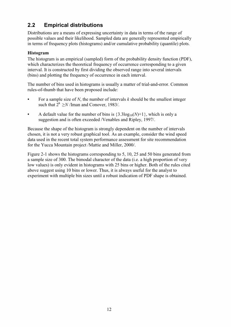
Because the shape of the histogram is strongly dependent on the number of intervals chosen, it is not a very robust graphical tool. As an example, consider the wind speed data used in the recent total system performance assessment for site recommendation for the Yucca Mountain project /Mattie and Miller, 2000/.
Figure 2-1 shows the histograms corresponding to 5, 10, 25 and 50 bins generated from a sample size of 300. The bimodal character of the data (i.e. a high proportion of very low values) is only evident in histograms with 25 bins or higher. Both of the rules cited above suggest using 10 bins or lower. Thus, it is always useful for the analyst to experiment with multiple bin sizes until a robust indication of PDF shape is obtained.
13
5 bins
Fre
quen
cy
0 500 1000 1500 2000 2500
020
4060
8012
0
10 bins
Fre
quen
cy
0 500 1000 1500 2000
010
2030
4050
60
25 bins
Fre
quen
cy
0 500 1000 1500 2000
010
2030
50 bins
Fre
quen
cy
0 500 1000 1500 2000
05
1015
2025
3035
Figure 2-1. Histograms showing sensitivity to bin size.
Quantile plot The quantile plot is an empirical (sampled) form of the cumulative distribution function (CDF), which characterizes the probability that a random variable is smaller than some specified value.
To construct a quantile plot, the data are first ranked in ascending order from the smallest (x1) to the largest (xN), where N is the number of samples. For each sorted value, xi, the quantile (cumulative frequency) is determined as qi = i/(N+1), and the quantile plot is generated by plotting qi versus xi. Percentiles are obtained by multiplying the quantile values by 100. The quantile plot is also referred to as an empirical CDF.
Unlike the histogram, the quantile plot is a much more robust tool for visualizing the fraction of samples which fall below a given value. It is also useful for determining if a distribution is symmetric or skewed.
14
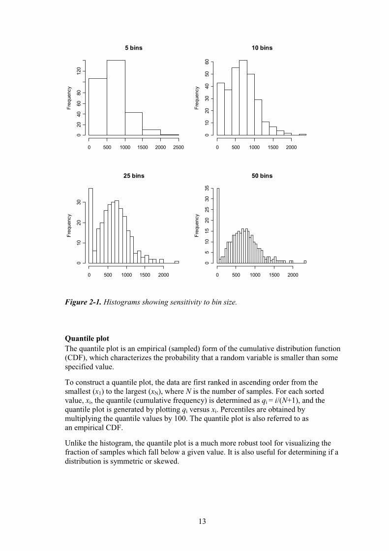
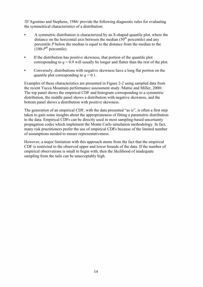
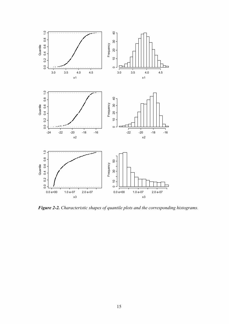
/D’Agostino and Stephens, 1986/ provide the following diagnostic rules for evaluating the symmetrical characteristics of a distribution:
• A symmetric distribution is characterized by an S-shaped quantile plot, where the distance on the horizontal axis between the median (50th percentile) and any percentile P below the median is equal to the distance from the median to the (100-Pth percentile).
• If the distribution has positive skewness, that portion of the quantile plot corresponding to q > 0.9 will usually be longer and flatter than the rest of the plot.
• Conversely, distributions with negative skewness have a long flat portion on the quantile plot corresponding to q < 0.1.
Examples of these characteristics are presented in Figure 2-2 using sampled data from the recent Yucca Mountain performance assessment study /Mattie and Miller, 2000/. The top panel shows the empirical CDF and histogram corresponding to a symmetric distribution, the middle panel shows a distribution with negative skewness, and the bottom panel shows a distribution with positive skewness.
The generation of an empirical CDF, with the data presented “as is”, is often a first step taken to gain some insights about the appropriateness of fitting a parametric distribution to the data. Empirical CDFs can be directly used in most sampling-based uncertainty propagation codes which implement the Monte Carlo simulation methodology. In fact, many risk practitioners prefer the use of empirical CDFs because of the limited number of assumptions needed to ensure representativeness.
However, a major limitation with this approach stems from the fact that the empirical CDF is restricted to the observed upper and lower bounds of the data. If the number of empirical observations is small to begin with, then the likelihood of inadequate sampling from the tails can be unacceptably high.
15
3.0 3.5 4.0 4.5
0.0
0.2
0.4
0.6
0.8
1.0
x1
Qua
ntile
x1
Fre
quen
cy
3.0 3.5 4.0 4.5
010
2030
40
-24 -22 -20 -18 -16
0.0
0.2
0.4
0.6
0.8
1.0
x2
Qua
ntile
x2
Fre
quen
cy
-22 -20 -18 -16
010
2030
40
0.0 e+00 1.0 e-07 2.0 e-07
0.0
0.2
0.4
0.6
0.8
1.0
x3
Qua
ntile
x3
Fre
quen
cy
0.0 e+00 1.0 e-07 2.0 e-07
010
3050
Figure 2-2. Characteristic shapes of quantile plots and the corresponding histograms.
16
2.3 Parametric models Parametric models of probability distributions are useful for several reasons:
• They provide a compact mathematical construct for summarizing empirical data.
• They allow extrapolation of data beyond the observed minimum and maximum values, as well as interpolation between sampled data points.
• They enable the statistical representation of uncertain quantities based on purely mechanistic considerations.
• They facilitate the Bayesian updating of distributions based on prior information.
Some of the common parametric models useful for performance assessment applications are described below. Here f(x) denotes the PDF, F(x) denotes the CDF, µ denotes the mean and σ denotes the standard deviation for the theoretical distribution assigned to the random variable of interest, x.
This discussion is based on standard references dealing with statistical applications in engineering and science /e.g. Ang and Tang, 1975; Benjamin and Cornell, 1970; Cullen and Frey, 1999; Hahn and Shapiro, 1967; Harr, 1987; Morgan and Henrion, 1990/. Also, topical examples are drawn from the recent total system performance assessment for site recommendation for the Yucca Mountain project /Mattie and Miller, 2000/.
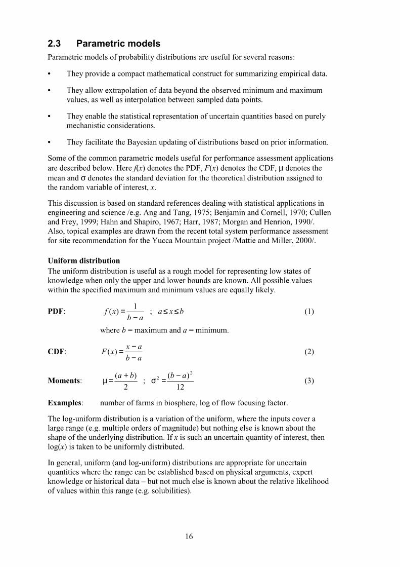
Uniform distribution The uniform distribution is useful as a rough model for representing low states of knowledge when only the upper and lower bounds are known. All possible values within the specified maximum and minimum values are equally likely.
PDF: bxaab
xf ≤≤−
= ;1
)( (1)
where b = maximum and a = minimum.
CDF: ab
axxF
−−=)( (2)
Moments: 12
)(;
2
)( 22 abba −=σ+=µ (3)
Examples: number of farms in biosphere, log of flow focusing factor.
The log-uniform distribution is a variation of the uniform, where the inputs cover a large range (e.g. multiple orders of magnitude) but nothing else is known about the shape of the underlying distribution. If x is such an uncertain quantity of interest, then log(x) is taken to be uniformly distributed.
In general, uniform (and log-uniform) distributions are appropriate for uncertain quantities where the range can be established based on physical arguments, expert knowledge or historical data – but not much else is known about the relative likelihood of values within this range (e.g. solubilities).
17
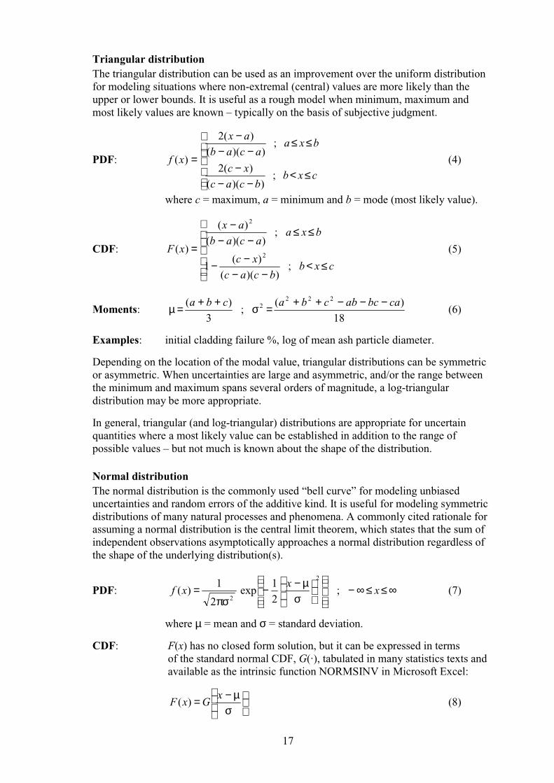
Triangular distribution The triangular distribution can be used as an improvement over the uniform distribution for modeling situations where non-extremal (central) values are more likely than the upper or lower bounds. It is useful as a rough model when minimum, maximum and most likely values are known – typically on the basis of subjective judgment.
PDF:
≤<−−
−
≤≤−−
−
=cxb
bcac
xc
bxaacab
ax
xf
;))((
)(2
;))((
)(2
)( (4)
where c = maximum, a = minimum and b = mode (most likely value).
CDF:
≤<−−
−−
≤≤−−
−
=cxb
bcac
xc
bxaacab
ax
xF
;))((
)(1
;))((
)(
)(2
2
(5)
Moments: 18
)(;
3
)( 2222 cabcabcbacba −−−++=σ++=µ (6)
Examples: initial cladding failure %, log of mean ash particle diameter.
Depending on the location of the modal value, triangular distributions can be symmetric or asymmetric. When uncertainties are large and asymmetric, and/or the range between the minimum and maximum spans several orders of magnitude, a log-triangular distribution may be more appropriate.
In general, triangular (and log-triangular) distributions are appropriate for uncertain quantities where a most likely value can be established in addition to the range of possible values – but not much is known about the shape of the distribution.
Normal distribution The normal distribution is the commonly used “bell curve” for modeling unbiased uncertainties and random errors of the additive kind. It is useful for modeling symmetric distributions of many natural processes and phenomena. A commonly cited rationale for assuming a normal distribution is the central limit theorem, which states that the sum of independent observations asymptotically approaches a normal distribution regardless of the shape of the underlying distribution(s).
PDF: ∞≤≤∞−
σµ−−
πσ= x
xxf ;
2
1exp
2
1)(
2
2 (7)
where µ = mean and σ = standard deviation.
CDF: F(x) has no closed form solution, but it can be expressed in terms of the standard normal CDF, G(·), tabulated in many statistics texts and available as the intrinsic function NORMSINV in Microsoft Excel:
σµ−= x
GxF )( (8)
18
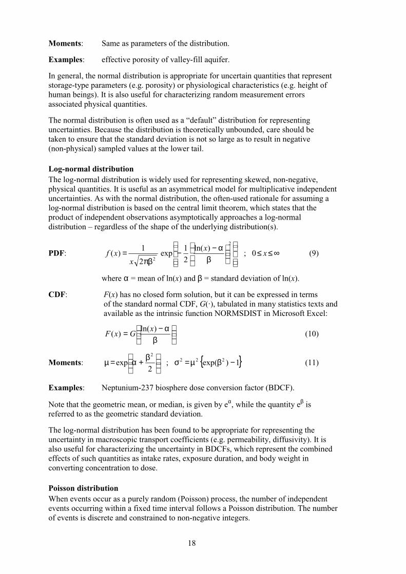
Moments: Same as parameters of the distribution.
Examples: effective porosity of valley-fill aquifer.
In general, the normal distribution is appropriate for uncertain quantities that represent storage-type parameters (e.g. porosity) or physiological characteristics (e.g. height of human beings). It is also useful for characterizing random measurement errors associated physical quantities.
The normal distribution is often used as a “default” distribution for representing uncertainties. Because the distribution is theoretically unbounded, care should be taken to ensure that the standard deviation is not so large as to result in negative (non-physical) sampled values at the lower tail.
Log-normal distribution The log-normal distribution is widely used for representing skewed, non-negative, physical quantities. It is useful as an asymmetrical model for multiplicative independent uncertainties. As with the normal distribution, the often-used rationale for assuming a log-normal distribution is based on the central limit theorem, which states that the product of independent observations asymptotically approaches a log-normal distribution – regardless of the shape of the underlying distribution(s).
PDF: ∞≤≤
β
α−−πβ
= xx
xxf 0;
)ln(
2
1exp
2
1)(
2
2 (9)
where α = mean of ln(x) and β = standard deviation of ln(x).
CDF: F(x) has no closed form solution, but it can be expressed in terms of the standard normal CDF, G(·), tabulated in many statistics texts and available as the intrinsic function NORMSDIST in Microsoft Excel:
β
α−= )ln()(
xGxF (10)
Moments: { }1)exp(;2
exp 2222
−βµ=σ
β+α=µ (11)
Examples: Neptunium-237 biosphere dose conversion factor (BDCF).
Note that the geometric mean, or median, is given by eα, while the quantity eβ is referred to as the geometric standard deviation.
The log-normal distribution has been found to be appropriate for representing the uncertainty in macroscopic transport coefficients (e.g. permeability, diffusivity). It is also useful for characterizing the uncertainty in BDCFs, which represent the combined effects of such quantities as intake rates, exposure duration, and body weight in converting concentration to dose.
Poisson distribution When events occur as a purely random (Poisson) process, the number of independent events occurring within a fixed time interval follows a Poisson distribution. The number of events is discrete and constrained to non-negative integers.
19
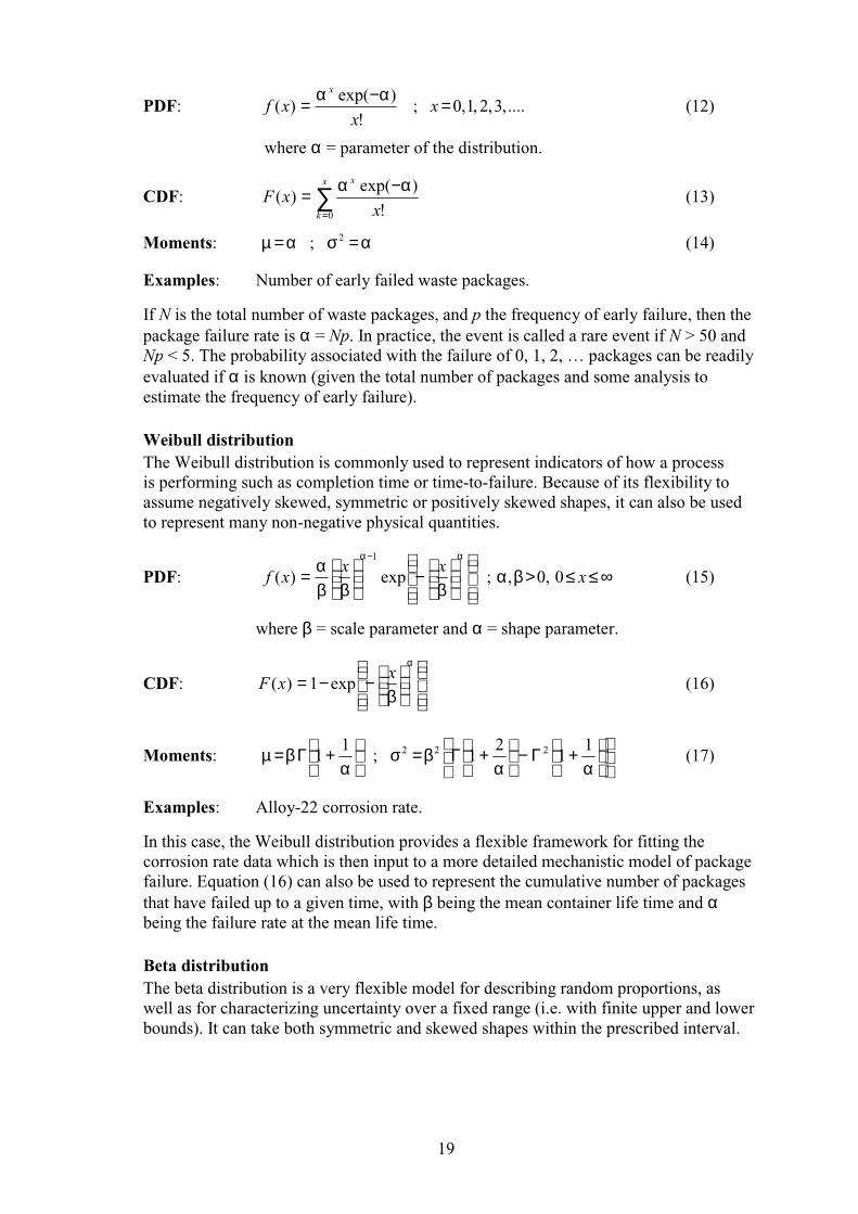
PDF: ....,3,2,1,0;!
)exp()( =α−α= x
xxf
x
(12)
where α = parameter of the distribution.
CDF: ∑=
α−α=x
k
x
xxF
0 !
)exp()( (13)
Moments: α=σα=µ 2; (14)
Examples: Number of early failed waste packages.
If N is the total number of waste packages, and p the frequency of early failure, then the package failure rate is α = Np. In practice, the event is called a rare event if N > 50 and Np < 5. The probability associated with the failure of 0, 1, 2, … packages can be readily evaluated if α is known (given the total number of packages and some analysis to estimate the frequency of early failure).
Weibull distribution The Weibull distribution is commonly used to represent indicators of how a process is performing such as completion time or time-to-failure. Because of its flexibility to assume negatively skewed, symmetric or positively skewed shapes, it can also be used to represent many non-negative physical quantities.
PDF: ∞≤≤>βα
β
−
ββ
α=α−α
xxx
xf 0,0,;exp)(1
(15)
where β = scale parameter and α = shape parameter.
CDF:
β
−−=α
xxF exp1)( (16)
Moments:
α+Γ−
α+Γβ=σ
α+Γβ=µ 1
12
1;1
1 222 (17)
Examples: Alloy-22 corrosion rate.
In this case, the Weibull distribution provides a flexible framework for fitting the corrosion rate data which is then input to a more detailed mechanistic model of package failure. Equation (16) can also be used to represent the cumulative number of packages that have failed up to a given time, with β being the mean container life time and α being the failure rate at the mean life time.
Beta distribution The beta distribution is a very flexible model for describing random proportions, as well as for characterizing uncertainty over a fixed range (i.e. with finite upper and lower bounds). It can take both symmetric and skewed shapes within the prescribed interval.
20
PDF: 10,0,;),(
)1()(
11
≤≤>βαβα
−=−β−α
xB
xxxf (18)
where α, β = distribution parameters and B(α,β)=Γ(α)Γ(β)/Γ(α+β).
CDF: F(x) has no closed form solution, but can be expressed using the intrinsic function BETADIST in Microsoft Excel.
Moments: )1()(
;2
2
+β+αβ+ααβ=σ
β+αα=µ (19)
Examples: Neptunium Kd in the saturated zone.
In this case, the beta distribution provides a flexible framework for characterizing the Neptunium Kd data. From mechanistic considerations, the beta distribution has also been recommended for fractional uncertain quantities (random proportions) such as the fraction of time individuals spend in various activities, partitioning of hazardous air pollutants in a power plant, etc /Cullen and Frey, 1999/.
Equation (18) characterizes a beta distribution with 0 and 1 as its lower and upper limits. It can be generalized for the case of arbitrary lower and upper bounds, denoted by a and b, as follows. Let X be a beta variable between 0 and 1, and Y be a beta variable between a and b. Then, the CDF and PDF of Y can be expressed in terms of the CDF and PDF of X by noting that:
Y = a + (b-a) X (20)
which leads to:
−−
−=
−−=
ab
ayf
abyf
ab
ayFyF
XY
XY
1)(
)(
(21)
These are the most commonly used distributions in probabilistic performance assessment studies. For a discussion of other theoretical parametric models, the reader is referred to any of the statistical texts cited at the beginning of this section.
21
2.4 Uncertainty and variability
Two important concepts are commonly encountered in the context of probabilistic modeling, i.e. uncertainty and variability. Uncertainty, also referred to as epistemic or subjective uncertainty, arises from lack of knowledge. Variability, also referred to as aleatory or stochastic uncertainty, arises due to natural randomness or heterogeneity.
Both uncertainty and variability may be quantified using probability distributions. However, the interpretation of the distributions differs in the two cases. The International Atomic Energy Agency /IAEA, 1989/ interprets distributions of variable quantities as representing the relative frequency of values from a specified interval – and distributions of uncertain quantities as representing the degree of belief that a known value is within a specified interval. Note that uncertainty can arise due to expert judgment for a quantity for which little data exists, as well as due to random sampling and measurement error.
/Morgan and Henrion, 1990/ suggest that variability is described by frequency distributions, and that uncertainty is described by probability distributions. The implication is that variability can be characterized via empirical distributions on the basis of data (and may subsequently be fitted to theoretical probability distributions). On the other hand, uncertainty is to be characterized on the basis of limited data and subjective judgment using theoretical probability distributions.
Uncertainty assessments in which input distributions commingle both variability and uncertainty yield a distribution of exposures applicable to a randomly selected individual. In this case, the assessment end point is the true but unknown distribution of doses among individuals in a population in which the individuals are selected from the population at random. This is also the approach to be taken if the mean dose for the population is to be evaluated for compliance demonstration.
If the primary objective of the analysis is an assessment of exposure to specific subpopulations (e.g. those in the upper percentiles of exposure), it may be necessary to separate uncertainty and variability. The model output in this case would be two-dimensional in nature (i.e. a family of dose versus exceedance probability curves), with the result being an uncertain estimate of the frequency distribution for variability in exposures to different members of the population. Thus, for any percentile of the population, there is some uncertainty about the actual exposure level. Conversely, at any selected exposure level, there is uncertainty about what fraction of the population is at or below this level.
/Frey and Burmaster, 1999/ describe a framework for characterizing uncertainty and variability on the basis of limited data. /Cullen and Frey, 1999/ discuss the use of multidimensional probabilistic analyses for propagating the effects of uncertainty and variability in order to produce uncertainty distributions for specific subpopulations.
23
3 Fitting continuous distributions
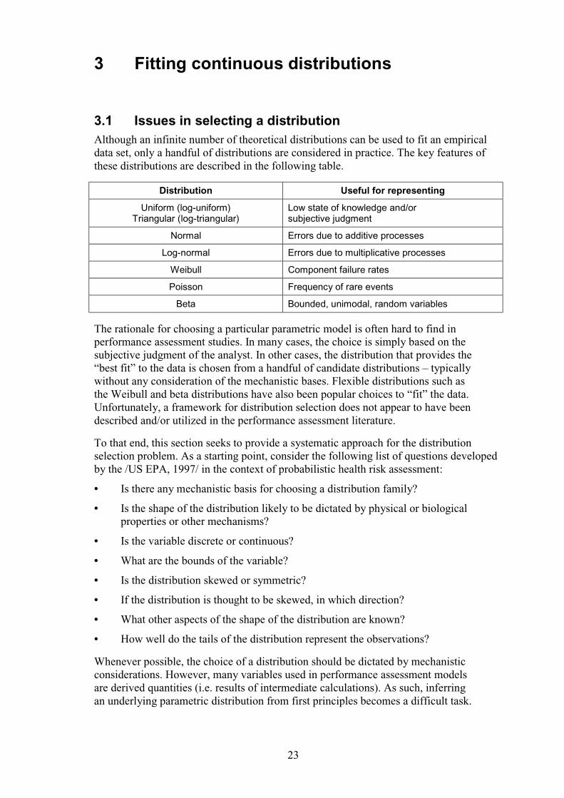
3.1 Issues in selecting a distribution Although an infinite number of theoretical distributions can be used to fit an empirical data set, only a handful of distributions are considered in practice. The key features of these distributions are described in the following table.
Distribution Useful for representing
Uniform (log-uniform) Triangular (log-triangular)
Low state of knowledge and/or subjective judgment
Normal Errors due to additive processes
Log-normal Errors due to multiplicative processes
Weibull Component failure rates
Poisson Frequency of rare events
Beta Bounded, unimodal, random variables
The rationale for choosing a particular parametric model is often hard to find in performance assessment studies. In many cases, the choice is simply based on the subjective judgment of the analyst. In other cases, the distribution that provides the “best fit” to the data is chosen from a handful of candidate distributions – typically without any consideration of the mechanistic bases. Flexible distributions such as the Weibull and beta distributions have also been popular choices to “fit” the data. Unfortunately, a framework for distribution selection does not appear to have been described and/or utilized in the performance assessment literature.
To that end, this section seeks to provide a systematic approach for the distribution selection problem. As a starting point, consider the following list of questions developed by the /US EPA, 1997/ in the context of probabilistic health risk assessment:
• Is there any mechanistic basis for choosing a distribution family?
• Is the shape of the distribution likely to be dictated by physical or biological properties or other mechanisms?
• Is the variable discrete or continuous?
• What are the bounds of the variable?
• Is the distribution skewed or symmetric?
• If the distribution is thought to be skewed, in which direction?
• What other aspects of the shape of the distribution are known?
• How well do the tails of the distribution represent the observations?
Whenever possible, the choice of a distribution should be dictated by mechanistic considerations. However, many variables used in performance assessment models are derived quantities (i.e. results of intermediate calculations). As such, inferring an underlying parametric distribution from first principles becomes a difficult task.
24
In these situations, a graphical analysis of the data using special probability plots can help identify candidate distributions (or at least eliminate inappropriate parametric models). Once a distribution has been selected, its parameters can then be estimated using one of several techniques discussed below. Also, statistical goodness-of-fit tests can be applied to further refine and/or validate the choice of distributions.
This sequence of: (a) hypothesizing a family of distributions, (b) estimating distribution parameters, and (c) assessing quality of fit of parameters is described in detail in the following sections. Illustrative examples are also provided for some of the more commonly used distributions.
3.2 Probability plots Probability plots are useful for comparing the data to postulated distributions. The observations are plotted, generally after some transformation, so that they would fall approximately on a straight line if the assumed parametric model was the “true” distribution from which the observations were sampled. Given that deviations from a straight line can be readily identified, probability plotting provides a straightforward visual screening tool for distribution selection /D’Agostino and Stephens, 1986/.
A visual examination of the probability plot will often help in determining whether the postulated distribution is appropriate or not. The analyst should also apply his or her knowledge of the process/parameter to verify that the agreement between the observations and the theoretical distribution is acceptable in key data regimes (e.g. high/low values). In mentally weighting different portions of the data differently, the analyst should be aware of deviations from the straight line which commonly occur at the tails due to the finite size of samples. Finally, the conclusions from a subjective assessment of the visualization of fit should be either: (a) the postulated model is adequate, (b) the model is questionable, or (c) the model is inadequate.
The starting point in probability plotting is an empirical CDF or quantile plot, where the quantiles (cumulative frequency) of the empirical distribution are plotted against the corresponding observations. Two common choices for defining the quantile, q, are the Weibull plotting position:
1+
=N
iqi (22)
and the Hazen plotting position:
N
iqi
5.0−= (23)
where i is the rank of the observation (sorted from smallest to largest) and N is the number of observations. Both of these approaches ensure that the minimum and maximum values of the sample are not assigned cumulative probabilities of 0 and 1, respectively. Other plotting positions may be derived from the general expression:
aN
aiqi 21−+
−= (24)
25
with 0 ≤ a ≤ 1 /D’Agostino and Stephens, 1986/. Although specific values of a have been recommended as optimal for different distributions, the most commonly used values correspond to a = 0 (Equation 22) and a = 0.5 (Equation 23).
A probability plot is a graph of the ranked observation, xi, versus an approximation of the expected value of the inverse CDF, F–1(qi). The relationships needed to construct probability plots for some of the common distributions are discussed below.
Normal distribution For the normal distribution, recall that the CDF, F(x), has no closed form solution, and is expressed in terms of the standard normal CDF, G(·):
=
σµ−= )()( zG
xGxF (25)
where z = (x – µ) / σ is the standard normal variate (also known as the z-score). This equation can be re-written as:
{ } ( )qGxFGx
z 11 )( −− ==σ
µ−= (26)
where the quantile, q, is used as an approximation of the cumulative probability, F. Rearranging, we obtain the following expression for a normal probability plot:
( )qGx 1−σ+µ= (27)
which suggests that a graph of x versus G–1(q), or z, should yield a straight line if the observed data follow a normal distribution. The straight line is characterized by a slope equal to the standard deviation, σ, and intercept equal to the mean, µ. Note that the inverse normal CDF, or the z-score, can be readily calculated using the intrinsic Microsoft Excel function, NORMSINV. Also, the quantile can be estimated from the ranks of the data using Equation (22) or Equation (23).
Log-normal distribution For a log-normal distribution, we define the standard normal variate as:
{ } ( )qGxFGx
z 11 )()ln( −− ==β
α−= (28)
where α = mean and β = standard deviation of ln(x). Re-arranging, we get:
( )qGx 1)ln( −β+α= (29)
Thus, a graph of ln(x) versus G–1(q), or z, should yield a straight line if the observed data follow a log-normal distribution. The straight line is characterized by a slope equal to the standard deviation, β, and an intercept equal to the mean, α, of the transformed variable ln(x). Note that the arithmetic mean and the arithmetic standard deviation can be readily obtained using Equation (11).
Weibull distribution For the Weibull distribution, re-arrangement of the CDF given in Equation (16) leads to:
( ){ } )ln()ln()1/(1lnln βα−α=− xq (30)
26
where the quantile, q, has been used to approximate the cumulative probability, F. Thus, a graph of ln(ln(1/(1–q))) versus ln(x) will produce a straight line if the observations are drawn from a Weibull distribution. The slope of the straight line is equal to the shape parameter, α. The scale parameter can be calculated from the slope and intercept as β = exp(-intercept/slope).
3.3 Parameter estimation techniques Once a candidate distribution has been selected for a data set, the parameters of the postulated theoretical distribution can be obtained in a variety of ways. The easiest approach (whenever possible) is to use linear regression in conjunction with probability plots. Additional techniques include the method of moments, maximum likelihood estimation or nonlinear least-squares analysis – as described below. In the next section, these techniques are demonstrated for various common probability distribution models using data from recent performance assessment studies carried out in the Yucca Mountain project.
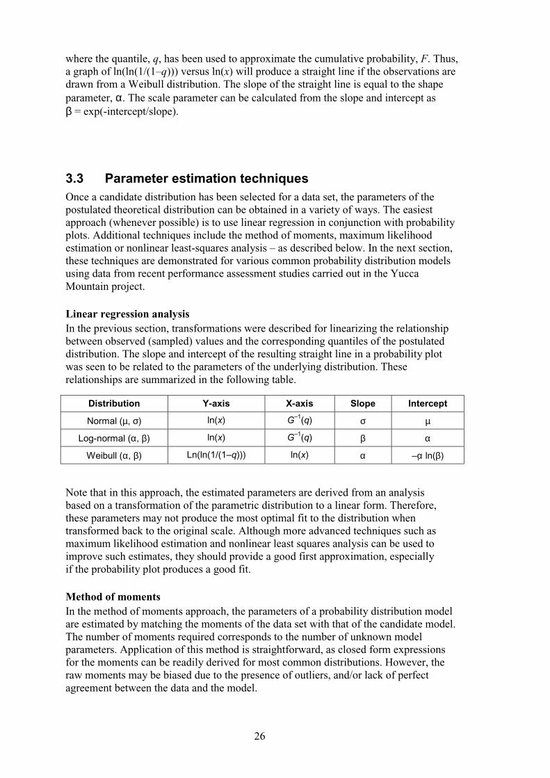
Linear regression analysis In the previous section, transformations were described for linearizing the relationship between observed (sampled) values and the corresponding quantiles of the postulated distribution. The slope and intercept of the resulting straight line in a probability plot was seen to be related to the parameters of the underlying distribution. These relationships are summarized in the following table.
Distribution Y-axis X-axis Slope Intercept
Normal (µ, σ) ln(x) G–1(q) σ µ
Log-normal (α, β) ln(x) G–1(q) β α
Weibull (α, β) Ln(ln(1/(1–q))) ln(x) α –α ln(β)
Note that in this approach, the estimated parameters are derived from an analysis based on a transformation of the parametric distribution to a linear form. Therefore, these parameters may not produce the most optimal fit to the distribution when transformed back to the original scale. Although more advanced techniques such as maximum likelihood estimation and nonlinear least squares analysis can be used to improve such estimates, they should provide a good first approximation, especially if the probability plot produces a good fit.
Method of moments In the method of moments approach, the parameters of a probability distribution model are estimated by matching the moments of the data set with that of the candidate model. The number of moments required corresponds to the number of unknown model parameters. Application of this method is straightforward, as closed form expressions for the moments can be readily derived for most common distributions. However, the raw moments may be biased due to the presence of outliers, and/or lack of perfect agreement between the data and the model.
27
Equations relating the theoretical first two moments (i.e. mean and variance) to distributional parameters are presented in Section 2.3. These provide the basis for estimating the parameters of the distribution from the sample moments (identified by the “hat” symbol) which are computed as follows:
( )∑
∑
=
=
µ−−
=σ
=µ
N
ii
N
ii
xN
xN
1
22
1
ˆ1
1ˆ
1ˆ
(31)
Method of moment estimators for some of the common distributions are:
Poisson: µ=α ˆ (32)
Normal: σ=σµ=µ ˆ;ˆ (33)
Log-normal: 2
)ˆln(;ˆ
ˆ1ln
2
2
22 β−µ=α
µσ+=β (34)
Beta: { }
2
22
2
232
ˆ
)ˆ1(ˆ)ˆ1(ˆ;
ˆ
)ˆˆˆˆ(
σµ−σ−µ−µ=β
σµσ−µ−µ=α (35)
Maximum likelihood estimation In the maximum likelihood estimation approach, a likelihood function is defined and the model parameters adjusted such that the corresponding likelihood of obtaining the observed data set is maximized.
As an example, consider the case of the normal distribution. The PDF for a normally distributed variable was given earlier in Equation (7), from which the likelihood function for a single, randomly drawn sample, xi, is inferred as:
∞≤≤∞−
σµ−
−πσ
=σµ xx
xp ii ;
21
exp2
1],|[
2
2 (36)
The likelihood function for drawing N-independent random samples is:
Likelihood [µ,σ| xi] =∏=
σµN
iixp
1
],|[ (37)
It is often more convenient to work with the log-likelihood, J, which can be expressed as a function of the two model parameters, µ and σ, as follows:
∑=
σµ−
−σ−π−=σµN
i
ixN
NJ
1
2
21
)ln()2ln(2
],[ (38)
The values of µ and σ which maximize the log-likelihood, J, are called the maximum likelihood estimates of the model parameters. This requires a nonlinear optimization algorithm, such as the SOLVER routine in Microsoft Excel.
28
/Frey and Burmaster, 1999/ provide examples of maximum likelihood parameter estimation for log-normal and beta distributions. In general, they note that maximum likelihood estimates do not always preserve the moments of the sample data.
Nonlinear least-squares analysis A more flexible approach involves the use of nonlinear least-squares analysis, where the goal is to estimate model parameters such that the mean squared difference between the observed and predicted CDF is minimized. This process can be readily implemented using the nonlinear optimization package SOLVER in Microsoft Excel.
1. Setup the data in a 2-column format, with the dependent variable being the observed quantile, qi, and the independent variable, being the observed value, xi.
2. Compute the sample moments, µ̂ and σ) .
3. Estimate the parameters of the postulated model from the sample moments using Equation 32–35. These will be used as initial guesses for the nonlinear regression.
4. Calculate the theoretical cumulative probability, Fi, using the appropriate form of the postulated parametric model as given in Section 2.3 and estimates of model parameters obtained from step 3.
5. Compute the difference between Fi and qi.
6. Setup SOLVER to minimize the sum of the squares of the differences in step 5, by adjusting the parameters estimated in step 3.
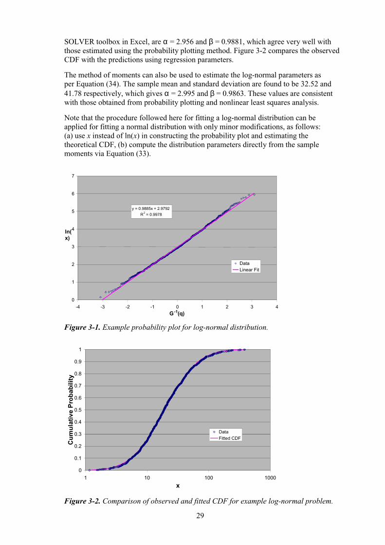
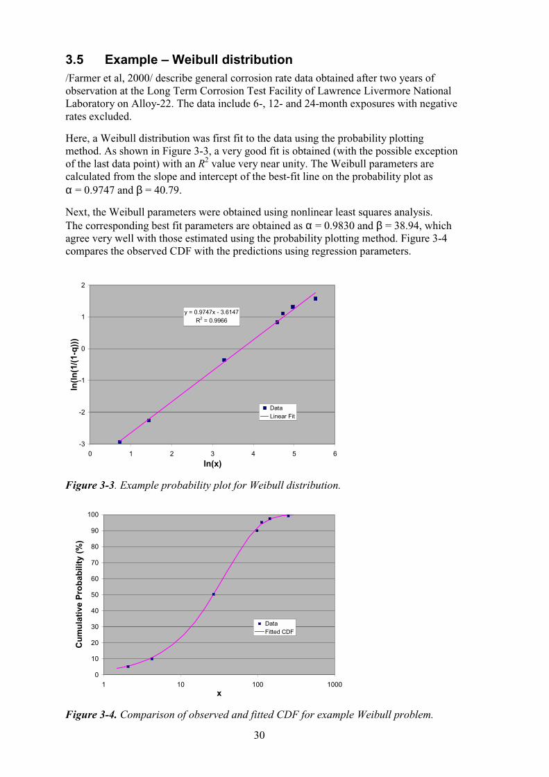
3.4 Example – log-normal distribution /Kuzio, 1999/ describes how observations on flowing interval spacing and fracture orientation were combined to correct for flowing intervals measured normal to the borehole. The observed distributions for flowing interval spacing, Fsm, and dip, Df, were discretized into 10-point CDFs, and then sampled 1000 times to obtain a distribution for the corrected flowing interval spacing, Fsmc, using the relationship Fsmc = Fsm cos(Df). These values were log-transformed and fit to a normal distribution, yielding a mean of 2.97 and a standard deviation of 0.99 for ln(Fsmc).
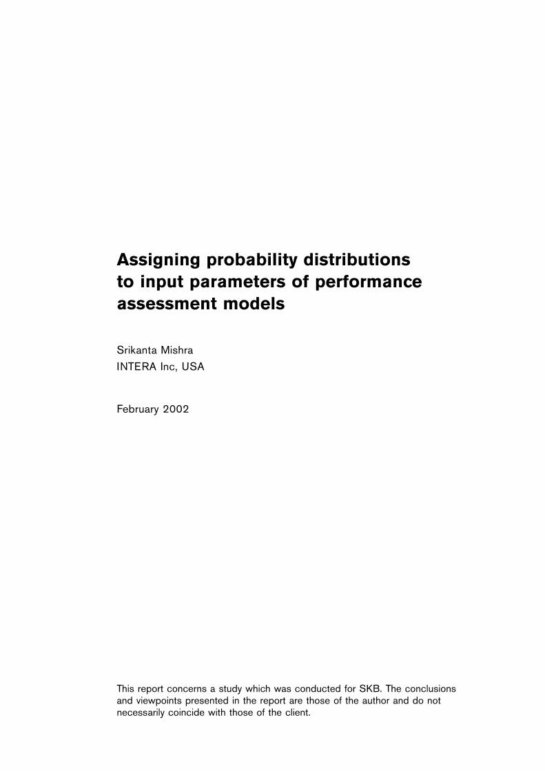
The calculation was repeated using the Monte Carlo simulation toolbox Crystal Ball to extract 1000 values of the corrected flowing interval spacing, Fsmc. A log-normal distribution was first fit to the data using the probability plotting method. This requires plotting the natural logarithm of Fsmc against the inverse of the standard normal CDF, G–1(q), where q is the quantile. As shown in Figure 3-1, a very good fit was obtained except at the extreme tails, with an R2 value approximately equal to 1. The log-normal parameters are calculated from the slope and intercept of the best-fit line on the probability plot as α = 2.979 and β = 0.9885.
Next, these parameters are obtained using nonlinear least-squares analysis, which requires minimizing the sum of the squared differences between the observed and the predicted quantiles corresponding to each observed value. The Excel function NORMSDIST was used to generate the standard normal CDF necessary for estimating the cumulative probability. The corresponding best fit parameters, obtained using the
29
SOLVER toolbox in Excel, are α = 2.956 and β = 0.9881, which agree very well with those estimated using the probability plotting method. Figure 3-2 compares the observed CDF with the predictions using regression parameters.
The method of moments can also be used to estimate the log-normal parameters as per Equation (34). The sample mean and standard deviation are found to be 32.52 and 41.78 respectively, which gives α = 2.995 and β = 0.9863. These values are consistent with those obtained from probability plotting and nonlinear least squares analysis.
Note that the procedure followed here for fitting a log-normal distribution can be applied for fitting a normal distribution with only minor modifications, as follows: (a) use x instead of ln(x) in constructing the probability plot and estimating the theoretical CDF, (b) compute the distribution parameters directly from the sample moments via Equation (33).
y = 0.9885x + 2.9792 R 2 = 0.9978
0
1
2
3
4
5
6
7
-4 -3 -2 -1 0 1 2 3 4 G -1 (q)
ln(x)
Data Linear Fit
Figure 3-1. Example probability plot for log-normal distribution.
0
0.1
0.2
0.3
0.4
0.5
0.6
0.7
0.8
0.9
1
1 10 100 1000
x
Cu
mu
lati
ve P
rob
abili
ty
DataFitted CDF
Figure 3-2. Comparison of observed and fitted CDF for example log-normal problem.
30
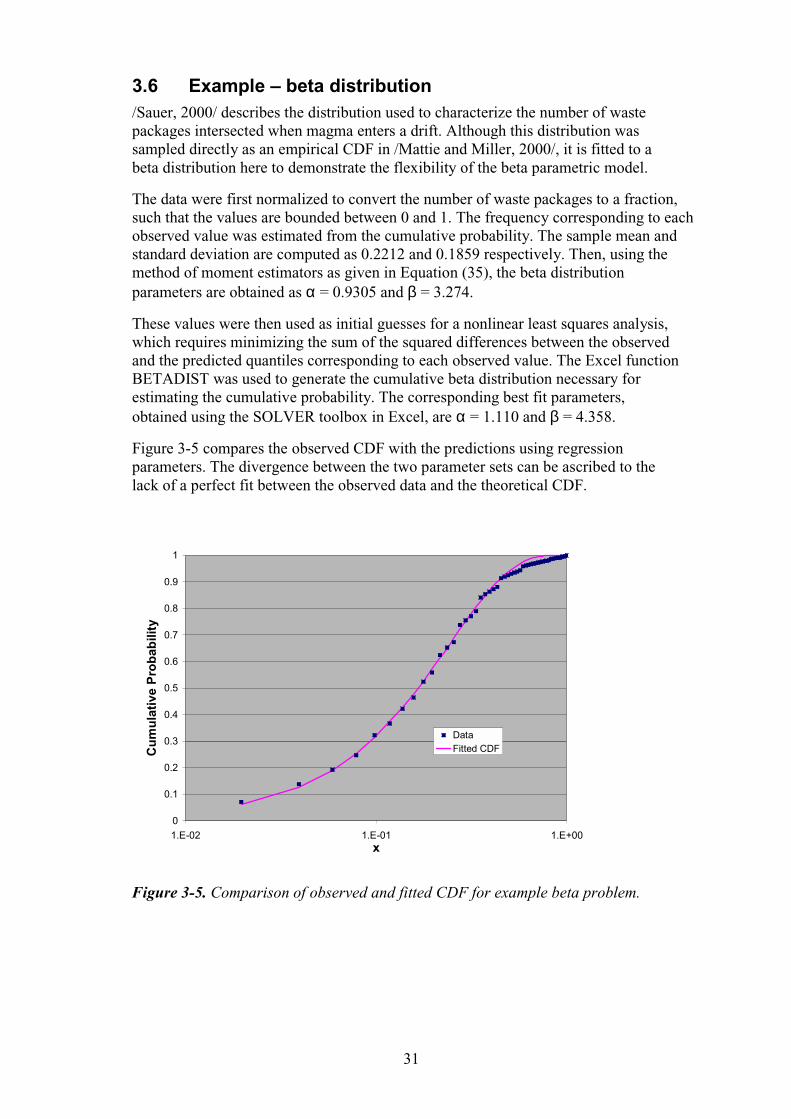
3.5 Example – Weibull distribution /Farmer et al, 2000/ describe general corrosion rate data obtained after two years of observation at the Long Term Corrosion Test Facility of Lawrence Livermore National Laboratory on Alloy-22. The data include 6-, 12- and 24-month exposures with negative rates excluded.
Here, a Weibull distribution was first fit to the data using the probability plotting method. As shown in Figure 3-3, a very good fit is obtained (with the possible exception of the last data point) with an R2 value very near unity. The Weibull parameters are calculated from the slope and intercept of the best-fit line on the probability plot as α = 0.9747 and β = 40.79.
Next, the Weibull parameters were obtained using nonlinear least squares analysis. The corresponding best fit parameters are obtained as α = 0.9830 and β = 38.94, which agree very well with those estimated using the probability plotting method. Figure 3-4 compares the observed CDF with the predictions using regression parameters.
y = 0.9747x - 3.6147R2 = 0.9966
-3
-2
-1
0
1
2
0 1 2 3 4 5 6
ln(x)
ln(l
n(1
/(1-
q))
)
DataLinear Fit
Figure 3-3. Example probability plot for Weibull distribution.
0
10
20
30
40
50
60
70
80
90
100
1 10 100 1000x
Cu
mu
lati
ve P
rob
abili
ty (
%)
DataFitted CDF
Figure 3-4. Comparison of observed and fitted CDF for example Weibull problem.
31
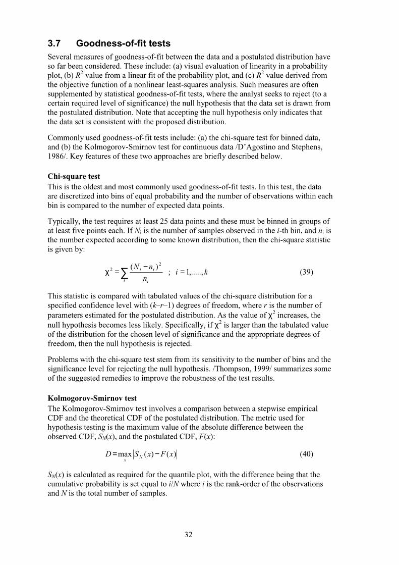
3.6 Example – beta distribution /Sauer, 2000/ describes the distribution used to characterize the number of waste packages intersected when magma enters a drift. Although this distribution was sampled directly as an empirical CDF in /Mattie and Miller, 2000/, it is fitted to a beta distribution here to demonstrate the flexibility of the beta parametric model.
The data were first normalized to convert the number of waste packages to a fraction, such that the values are bounded between 0 and 1. The frequency corresponding to each observed value was estimated from the cumulative probability. The sample mean and standard deviation are computed as 0.2212 and 0.1859 respectively. Then, using the method of moment estimators as given in Equation (35), the beta distribution parameters are obtained as α = 0.9305 and β = 3.274.
These values were then used as initial guesses for a nonlinear least squares analysis, which requires minimizing the sum of the squared differences between the observed and the predicted quantiles corresponding to each observed value. The Excel function BETADIST was used to generate the cumulative beta distribution necessary for estimating the cumulative probability. The corresponding best fit parameters, obtained using the SOLVER toolbox in Excel, are α = 1.110 and β = 4.358.
Figure 3-5 compares the observed CDF with the predictions using regression parameters. The divergence between the two parameter sets can be ascribed to the lack of a perfect fit between the observed data and the theoretical CDF.
0
0.1
0.2
0.3
0.4
0.5
0.6
0.7
0.8
0.9
1
1.E-02 1.E-01 1.E+00x
Cu
mu
lati
ve P
rob
abili
ty
DataFitted CDF
Figure 3-5. Comparison of observed and fitted CDF for example beta problem.
32
3.7 Goodness-of-fit tests Several measures of goodness-of-fit between the data and a postulated distribution have so far been considered. These include: (a) visual evaluation of linearity in a probability plot, (b) R2 value from a linear fit of the probability plot, and (c) R2 value derived from the objective function of a nonlinear least-squares analysis. Such measures are often supplemented by statistical goodness-of-fit tests, where the analyst seeks to reject (to a certain required level of significance) the null hypothesis that the data set is drawn from the postulated distribution. Note that accepting the null hypothesis only indicates that the data set is consistent with the proposed distribution.
Commonly used goodness-of-fit tests include: (a) the chi-square test for binned data, and (b) the Kolmogorov-Smirnov test for continuous data /D’Agostino and Stephens, 1986/. Key features of these two approaches are briefly described below.
Chi-square test This is the oldest and most commonly used goodness-of-fit tests. In this test, the data are discretized into bins of equal probability and the number of observations within each bin is compared to the number of expected data points.
Typically, the test requires at least 25 data points and these must be binned in groups of at least five points each. If Ni is the number of samples observed in the i-th bin, and ni is the number expected according to some known distribution, then the chi-square statistic is given by:
∑ =−
=χi i
ii kin
nN,.....,1;
)( 22 (39)
This statistic is compared with tabulated values of the chi-square distribution for a specified confidence level with (k–r–1) degrees of freedom, where r is the number of parameters estimated for the postulated distribution. As the value of χ2 increases, the null hypothesis becomes less likely. Specifically, if χ2 is larger than the tabulated value of the distribution for the chosen level of significance and the appropriate degrees of freedom, then the null hypothesis is rejected.
Problems with the chi-square test stem from its sensitivity to the number of bins and the significance level for rejecting the null hypothesis. /Thompson, 1999/ summarizes some of the suggested remedies to improve the robustness of the test results.
Kolmogorov-Smirnov test The Kolmogorov-Smirnov test involves a comparison between a stepwise empirical CDF and the theoretical CDF of the postulated distribution. The metric used for hypothesis testing is the maximum value of the absolute difference between the observed CDF, SN(x), and the postulated CDF, F(x):
)()(max xFxSD Nx
−= (40)
SN(x) is calculated as required for the quantile plot, with the difference being that the cumulative probability is set equal to i/N where i is the rank-order of the observations and N is the total number of samples.
33
The null hypothesis is tested by comparing the value of D with the tabulated value of the test statistic for the selected level of significance and the number of samples. For a significance level of 0.05, the critical D value can be estimated as 1.36/√N for a sample size greater than 50.
The Kolmogorov-Smirnov test tends to be most sensitive around the median and less sensitive at the extreme ends of the distribution. If a better fit is desired at the tails of the distribution rather than at the mid-range, an alternative goodness-of-fit test is the Anderson-Darling test, with the following test statistic:
[ ])(1)(
)()(max*
xFxF
xFxSD N
x −
−= (41)
In general, all goodness-of-fit tests require some subjectivity – especially in choosing the level of significance. As such, it is not appropriate to use them in an automated manner for selecting a distribution which provides the “best” fit to the data. Rather, the approach should be to use goodness-of-fit tests in conjunction with probability plots and an understanding of the underlying mechanisms (governing the uncertain quantity of interest) to evaluate the adequacy of the postulated distribution(s).
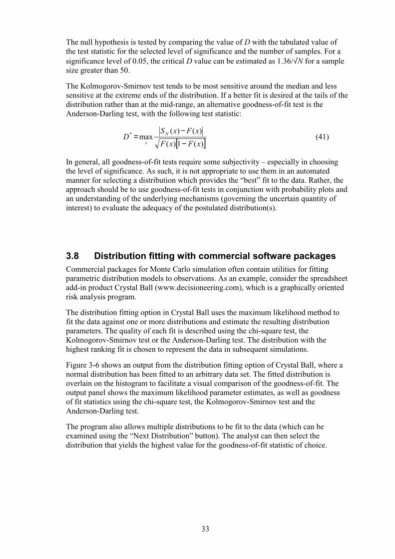
3.8 Distribution fitting with commercial software packages Commercial packages for Monte Carlo simulation often contain utilities for fitting parametric distribution models to observations. As an example, consider the spreadsheet add-in product Crystal Ball (www.decisioneering.com), which is a graphically oriented risk analysis program.
The distribution fitting option in Crystal Ball uses the maximum likelihood method to fit the data against one or more distributions and estimate the resulting distribution parameters. The quality of each fit is described using the chi-square test, the Kolmogorov-Smirnov test or the Anderson-Darling test. The distribution with the highest ranking fit is chosen to represent the data in subsequent simulations.
Figure 3-6 shows an output from the distribution fitting option of Crystal Ball, where a normal distribution has been fitted to an arbitrary data set. The fitted distribution is overlain on the histogram to facilitate a visual comparison of the goodness-of-fit. The output panel shows the maximum likelihood parameter estimates, as well as goodness of fit statistics using the chi-square test, the Kolmogorov-Smirnov test and the Anderson-Darling test.
The program also allows multiple distributions to be fit to the data (which can be examined using the “Next Distribution” button). The analyst can then select the distribution that yields the highest value for the goodness-of-fit statistic of choice.
34
Figure 3-6. Distribution fitting output from Crystal Ball.
3.9 Does the choice of distributions matter? A common concern in Monte Carlo analysis is the effect of distribution choice for uncertain parameters on the outcome of the analysis. /Hoffman, 1996/ presented a study of the sensitivity of model outcomes to distribution shape for a variety of model structures and distributions. His conclusions can be summarized as follows:
• As long as the uncertainty of a given parameter is small (CV ≤ 30%), it makes very little difference which distribution is chosen.
• As the coefficient of variation approaches and exceeds 30%, the use of distributions of log-transformed values is recommended.
• Choice of distribution shape will be important if we are interested in extreme values.
A rigorous analysis of the sensitivity of probabilistic model results to distribution shape requires multiple Monte Carlo runs, each carried out with a different probability distribution for the parameter of interest. This is often impractical.
An alternative computational scheme without recourse to additional simulations has been proposed for this purpose /Iman, 1980/. The method involves a mapping of the original sampled values onto the space of the new distribution to compute a modified set of weights, which are then used for re-weighting the computed outcomes. /RamaRao et al, 2001/ describe an application of this procedure and note good agreement between the proposed re-weighting scheme and re-simulation results.
35
4 Subjective assessment of probabilities
4.1 Maximum entropy distribution selection Although it is desirable to generate probability distributions for uncertain parameters on the basis of observed and/or simulated data, reality does not always cooperate with the analyst in this regard. Distributions are therefore routinely inferred on the basis of only a limited amount of information and are also subject to rather ad-hoc assumptions. As an alternative, the principle of maximum entropy offers a systematic approach to distribution selection under such conditions.
It is well known that the concept of thermodynamic entropy is related to the degree of disorder. Similarly, the concept of “information” entropy may be used to characterize the uncertainty of probability states, viz:
)ln( ii
i ppH ∑−= (42)
where H is the Shannon entropy (so named after its original proponent), and pi is the probability associated with the i-th sample. It is easily shown that the maximum entropy corresponds to a uniform distribution (where all samples are equally likely). Any other distribution would have a concentration of probability away from the extreme values, leading to a reduction of uncertainty and hence a reduction of entropy.
The principle of maximum entropy seeks to choose a PDF which maximizes the entropy, subject to known constraints. Uncertainty is reduced as much as possible by using all information (i.e. satisfying all constraints), but no further by unnecessary assumptions. This ensures that ignorance is preserved and one is maximally uncertain with respect to the unknown information.
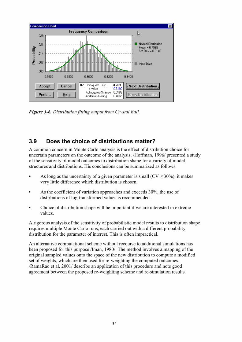
/Harr, 1987/ discusses how the maximum entropy principle can help assign probability distributions on the basis of known constraints, as per the following table.
Constraint Assigned PDF
Upper bound, lower bound Uniform
Minimum, maximum, mode Triangular
Mean, standard deviation Normal
Range, mean, std. Dev. Beta
Mean occurrence rate Poisson
As an example, consider the situation when only the lower and upper bounds for an uncertain parameter are known. The principle of maximum entropy would indicate a uniform distribution. One could opt for a triangular distribution, where the mode is taken as the mid-point of the range. However, that would be tantamount to making assumptions not supported by the data. Thus, the entropy-based distribution selection framework forces the analyst to be maximally uncertain about the data.
36
4.2 Generation of subjective probability distributions Another common strategy employed in the absence of data is to ask subject matter experts to develop distributions representing their degree of belief regarding the uncertain quantity of interest. It is generally recommended /Ang and Tang, 1975; Helton, 1993/ that distributions are best developed by specifying selected percentile values, rather than trying to specify a particular parametric distribution model (e.g. normal) and its associated parameters (e.g. mean, standard deviation).
For example, one starts by specifying the minimum, the maximum and the median values – which correspond to the 0th, 100th and 50th percentiles. The distribution is refined by adding intermediate percentiles such as the 10th and 90th, the 25th and 75th, etc. Plotting the empirical CDF also helps in deciding whether the selected values at given percentiles need to be adjusted, and/or additional percentiles need to be added. In general, it is easier for experts to defend the choice of values corresponding to selected percentiles than the choice of parameters characterizing a parametric distribution model.
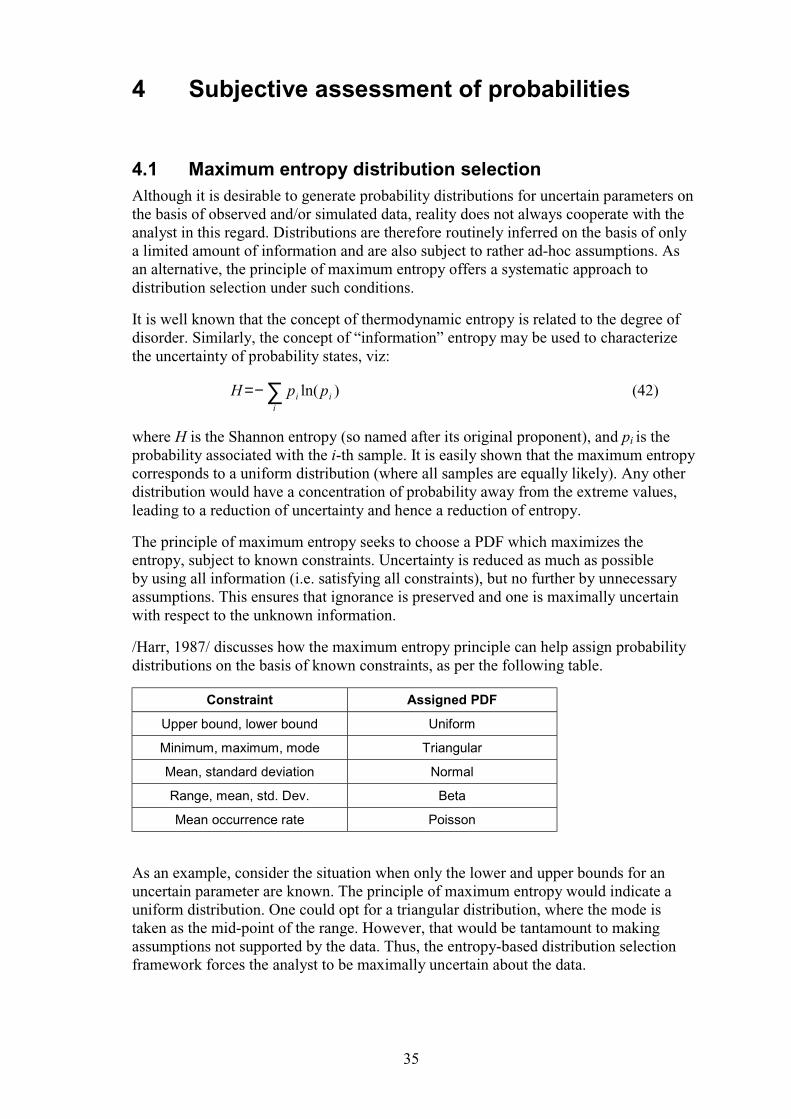
An example of such a subjective distribution is that elicited for the Neptunium Kd for the alluvial deposits of the saturated zone at Yucca Mountain. The expert was Dr. Donald Langmuir, a member of the saturated zone expert elicitation panel for the total system performance assessment in support of viability assessment /US DOE, 1998/. Taking into account available data as well as the uncertainty in the mineralogy, Dr. Langmuir proposed the following CDF.
Kd (mL/g) Percentile of CDF
1000 100%
100 95%
40 50%
10 10%
1 0%
When many uncertain quantities are candidates for subjective probability distributions, it is not worthwhile spending limited resources to develop such distributions for each and every parameter. /Helton, 1993/ suggests a two-step procedure, wherein all variables are first crudely characterized as uniform (or log-uniform, depending on the range) distributions for a screening-level analysis. Model results are analyzed to identify the most important contributors to output uncertainty. Resources can then be focused on this subset of parameters for a more detailed characterization of uncertainty prior to the second-level analysis. Simplified performance assessment models /e.g. Hedin, 2002/ are ideal for such screening calculations.
37
4.3 Formal expert elicitation protocols In the previous section, a methodology for informally codifying expert judgment (without structured efforts to control biases) was presented. However, in matters important to the demonstration of compliance, the application of formal expert elicitation should be considered whenever one or more of the following conditions exist /Kotra et al, 1996/:
• Empirical data are not reasonably obtainable, and/or the analyses are not practical to perform because of time or cost constraints.
• Uncertainties are large and significant to the demonstration of compliance.
• More than one conceptual model can explain, or be consistent with, available data.
• Technical judgments are required to assess whether bounding assumptions or calculations are appropriately conservative.
Formal protocols for expert elicitation have been developed in the field of decision analysis /Morgan and Henrion, 1990/, and have also been applied extensively to quantify the uncertainty in risk associated with nuclear power generation /Hora and Iman, 1989; NCRP, 1996/. In addition, the US DOE has recently developed guidance for the formal use of expert judgment by the Yucca Mountain Project /US DOE, 1995/, and the US NRC staff has issued a branch technical position on the use of expert elicitation in the high-level waste program /Kotra et al, 1996/.
The main motivation for using a consistent and systematic procedure during formal elicitation of expert judgment is to ensure that the results obtained accurately reflect what is known (as well as what is not known) about the topic in question. The necessary components in an expert elicitation process can be described as follows /Kotra et al, 1996/.
Step No. 1 – Definition of objectives The objectives of the elicitation should be defined explicitly and in a manner that reflects a clear understanding of how the judgments obtained will be used.
Step No. 2 – Selection of experts The elicitation team consists of a group of generalists and normative experts conducting and facilitating the elicitation, in addition to the subject-matter experts. Generalists are individuals with substantial technical background in one or more of the disciplines needed to solve the problem of interest. Normative experts have a sound theoretical and conceptual knowledge of probability and practical experience in expert elicitation.
Subject-matter experts selected for the elicitation should be individuals who: (a) possess the necessary knowledge and expertise, (b) have demonstrated their ability to apply their knowledge and expertise, (c) represent a broad diversity of independent opinion and approaches for addressing the topics in question, (d) are willing to be identified publicly with their judgments, and (e) are willing to publicly disclose all conflicts of interest.
Step No. 3 – Identification of issues and problem decomposition The generalists and normative experts should work with the subject-matter experts to decompose the broad objectives of the elicitation by clearly and precisely specifying more focused and simpler sub-issues.
38
Step No. 4 – Assembly and dissemination of basic information Assembly of background information (in a complete and unbiased manner) should be initially conducted by the generalists and the normative experts. As the elicitation process proceeds, the subject-matter experts may be able to recommend additional sources of information.
Step No. 5 – Pre-elicitation training The expert panel should be provided training before the elicitations to: (a) familiarize them with the subject matter, (b) familiarize them with the elicitation process, (c) educate them with both uncertainty and probability encoding, (d) provide them practice in formally articulating their judgments and the underlying assumptions, (e) educate them with possible biases that could be present and influence their judgment.
Step No. 6 – Elicitation of judgments The individual elicitation sessions should be held in private, with the generalists and normative experts in attendance. All subject-matter experts should be queried in a uniform manner and asked to provide specific answers to questions about the issues considered and the reasoning behind their responses.
Step No. 7 – Post-elicitation feedback Each subject-matter expert should be provided feedback from the elicitation team on the results of his or her elicitation after the elicitation sessions are completed. Each expert should be queried as to the need for revision or clarification of his or her judgment.
Step No. 8 – Aggregation of judgments Whatever aggregation method is employed, the individual expert’s opinions must be preserved and documented. Transparency in the aggregation process will render these judgments, including disparate views or outliers, useful for subsequent analyses. Subject matter experts with differing views should be asked to comment on opposing views. Should the disparity in views persist, then each of the significantly varying views should be provided as output of the elicitation.
Step No. 9 – Documentation The specific issues addressed by the elicitation should be precisely defined along with all relevant definitions and assumptions. Results of the expert elicitation should be clearly described together with the reasoning supporting the judgments. The documentation should also distinguish between the information directly provided by the subject-matter experts and any subsequent processing of that information (e.g. smoothing, aggregation).
4.4 Case study – expert elicitation in Yucca Mountain project
A series of formal expert elicitations were carried out in support of the total system performance assessment for viability assessment of the Yucca Mountain project /US DOE, 1998/. These expert elicitations focused on the following process models: (a) unsaturated zone flow, (b) waste package degradation, (c) saturated zone flow and transport, (d) waste form degradation and radionuclide mobilization, and (e) near field and altered zone coupled processes. Experts from within and outside the Yucca Mountain project were consulted to assist in the synthesis of knowledge, identification

39
of data gaps and uncertainty quantification on those issues of greatest importance to the performance assessment process.
The expert elicitations were conducted in a structured step-wise approach as follows /Coppersmith et al, 1998/:
• Development of project plan: The goals and key elements of the project, timing and scope of significant activities such as workshops, significant milestones, etc were outlined by the methodology development team.
• Selection of the expert panel: For each panel, 5–6 experts (each with significant professional stature and technical expertise) were selected by the methodology development team on the advice of highly regarded scientists and engineers.
• Data compilation and dissemination: Pertinent data, including published reference materials, were compiled and sent to the experts.
• Meetings of the expert panel: Structured, facilitated interaction among the members of the expert panel took place during three workshops and one field trip (for each of the five elicitations). The workshops were designed to identify significant issues, available data, alternative models and uncertainties related to each process model. Pertinent data sets and alternative interpretations were presented by project staff and stakeholders to provide multiple points of view.
• Elicitation of experts: One-day individual elicitation interviews were held to obtain each expert’s assessments of the key issues, quantification of uncertainties and technical basis for the assessment. The interview was documented by the elicitation team for subsequent review and/or revision by the individual experts.
• Feedback of preliminary results: Elicitation summaries from all members of the expert panel were distributed to each expert to provide them with a broader perspective on the range of interpretations being developed.
• Finalization of expert assessments: After reviewing the feedback package, the experts developed a final draft of their elicitation summary.
• Preparation of project report: A report was developed for each process model to document the process followed, the expert elicitation summaries, and the results.
The outcomes of these expert elicitations were both quantitative and qualitative in nature. Quantitative estimates of uncertainty included PDFs for important parameters such as percolation flux, waste package corrosion rates, saturated zone dispersivity and waste form dissolution rates. Qualitative expressions of uncertainties in conceptual models covered such issues as explanations for fast-flow paths, fracture-matrix interaction, corrosion models of various waste package alloys, changes in hydraulic properties due to thermal effects, and dilution mechanisms in the saturated zone.
41
5 Bayesian updating
5.1 Bayes theorem In classical or “frequentist” statistics, probability is defined as the frequency of occurrence observed over a long series of independent trials. An alternative point of view is provided by subjective or “Bayesian” statistics, where the concept of probability is treated as the degree of belief – given all information.
Probability statements by frequentists are thus firmly rooted in data, which may not be available or may be inappropriate for the problem at hand. On the other hand, Bayesians are allowed to work with all information, which can include both subjective knowledge as well as “hard” measurements. A formal methodology for combining prior knowledge with current data to produce an updated distribution follows from Bayes theorem.
The theorem of Bayes, normally used for expressing the conditional probability of an event occurring, given that another event has occurred, can be adapted for the probability distribution updating problem as follows:
( )∫ θθ
θθ=θ|)(
)|()()|(
zPP
zPPzP (43)
where P(θ) is the prior distribution of the random variable θ, P(z|θ) is the probability model, or likelihood function, for the observed data z given θ, and P(θ|z) is the posterior distribution for θ given that the data z have been observed.
This compact formula provides a powerful construct for integrating old and new information in a systematic manner. It facilitates the explicit use of prior test data or consensus engineering judgment to “adjust” new data and potentially account for unquantified uncertainties.
The solution of Equation (42) for practical applications is a non-trivial task, especially because of the integral in the denominator. Closed-form analytical expressions can only be derived for a few special cases. Specifically, if P(θ|z) and P(θ) both belong to the same distribution family, then P(θ) and P(z|θ) are called conjugate distributions, and P(θ) is called the conjugate prior for P(z|θ). For certain conjugate pairs, the computation of the posterior distribution reduces to a simple arithmetic operation involving the parameters of the prior distribution and the likelihood function. Relationships for common conjugate pairs are discussed in detail elsewhere /DeGroot, 1970/, and are summarized below.
Observations Prior Posterior
Bernoulli Beta Beta
Poisson Gamma Gamma
Negative Binomial Normal Normal
Normal Normal Normal
Normal Gamma Gamma
42
For most other cases, a numerical integration approach based on advanced sampling techniques has to be used for developing the posterior distribution. However, for many engineering problems, a satisfactory solution can be achieved by taking an enumerative approach, where a continuous probability distribution is discretized into a collection of mutually independent outcome states prior to the application of Equation (43). This reduces the integral in the denominator to a simple summation. This is the approach adopted for the example problem discussed in the next section.
5.2 Example of Bayesian updating /Wilson, 2000/ describes the development of parameters for a seepage model based on numerical simulations of flow to a drift. The seepage model has two parameters, seepage fraction, fs, and seep flow rate, Qs. The seepage fraction describes the proportion of drifts where seepage occurs, and the seep flow rate describes the corresponding seepage flux. Both of these quantities are functions of the percolation flux, q. Using a limited number of detailed 3-dimensional simulations of flow to a drift, /Wilson, 2000/ developed uncertainty distributions for fs and Qs at various discrete values of q. These distributions were subsequently adjusted to account for processes such as drift degradation, flow focusing and coupled effects.
An application of the Bayesian updating framework is demonstrated for this problem by treating fs as the parameter of interest for which some prior information is available. The objective is to provide a posterior distribution by combining this prior distribution with new information as generated by the analysis reported in /Wilson, 2000/.
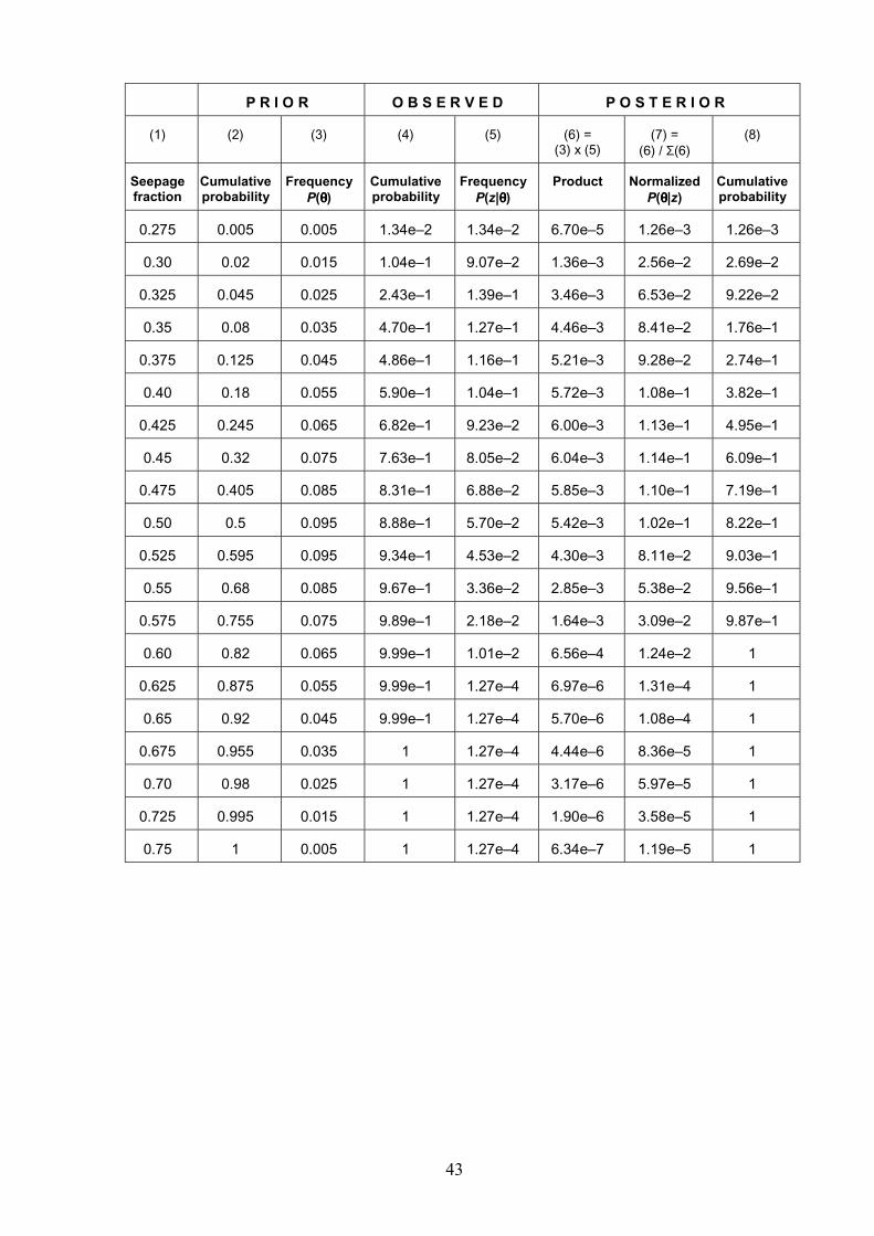
Assume that in the absence of any pertinent data, and based strictly on expert judgment, the uncertainty in fs (at a percolation flux q = 1000 mm/yr) can be treated as a triangular distribution with minimum = 0.25, mode = 0.50 and maximum = 0.75. This is the “prior” distribution. For Bayesian computations, the range of possible values is first divided into 20 equally-spaced intervals. The cumulative probability corresponding to each of these intervals is computed using Equation (5), from which the frequency is calculated by taking the difference between two successive cumulative probabilities. The computed frequency is P(θ) in the notation of Equation (43), and is shown in Column 3 of the following table.
The next step is to estimate the frequency corresponding to these probability states (i.e. binned intervals) from Wilson’s results. His analysis suggests a triangular distribution with minimum = 0.261, mode = 0.303 and maximum = 0.609 can be used to describe the data. As before, Equation 5 is used to compute the cumulative probability (and hence, the frequency) for each of the bins. The computed frequency is P(z|θ) in the notation of Equation (43), and is shown in Column 5 of the following table.
For each of the binned intervals, the “posterior” probability, P(θ|z), is then computed using Bayes theorem by taking the product of P(θ) and P(z|θ), and normalizing it by the sum of all P(θ) and P(z|θ) pairs (i.e. 5.31e–2). This is shown in Column 7 of the following table. Figure 5-1 presents a graphical comparison of the prior and posterior distributions. Note how the updated distribution has resulted in a reduction in variance (because of the addition of new information).
43
P R I O R O B S E R V E D P O S T E R I O R
(1) (2) (3) (4) (5) (6) = (3) x (5)
(7) = (6) / Σ(6)
(8)
Seepage fraction
Cumulative probability
Frequency P(θθθθ)
Cumulative probability
Frequency P(z|θθθθ)
Product Normalized P(θθθθ|z)
Cumulative probability
0.275 0.005 0.005 1.34e–2 1.34e–2 6.70e–5 1.26e–3 1.26e–3
0.30 0.02 0.015 1.04e–1 9.07e–2 1.36e–3 2.56e–2 2.69e–2
0.325 0.045 0.025 2.43e–1 1.39e–1 3.46e–3 6.53e–2 9.22e–2
0.35 0.08 0.035 4.70e–1 1.27e–1 4.46e–3 8.41e–2 1.76e–1
0.375 0.125 0.045 4.86e–1 1.16e–1 5.21e–3 9.28e–2 2.74e–1
0.40 0.18 0.055 5.90e–1 1.04e–1 5.72e–3 1.08e–1 3.82e–1
0.425 0.245 0.065 6.82e–1 9.23e–2 6.00e–3 1.13e–1 4.95e–1
0.45 0.32 0.075 7.63e–1 8.05e–2 6.04e–3 1.14e–1 6.09e–1
0.475 0.405 0.085 8.31e–1 6.88e–2 5.85e–3 1.10e–1 7.19e–1
0.50 0.5 0.095 8.88e–1 5.70e–2 5.42e–3 1.02e–1 8.22e–1
0.525 0.595 0.095 9.34e–1 4.53e–2 4.30e–3 8.11e–2 9.03e–1
0.55 0.68 0.085 9.67e–1 3.36e–2 2.85e–3 5.38e–2 9.56e–1
0.575 0.755 0.075 9.89e–1 2.18e–2 1.64e–3 3.09e–2 9.87e–1
0.60 0.82 0.065 9.99e–1 1.01e–2 6.56e–4 1.24e–2 1
0.625 0.875 0.055 9.99e–1 1.27e–4 6.97e–6 1.31e–4 1
0.65 0.92 0.045 9.99e–1 1.27e–4 5.70e–6 1.08e–4 1
0.675 0.955 0.035 1 1.27e–4 4.44e–6 8.36e–5 1
0.70 0.98 0.025 1 1.27e–4 3.17e–6 5.97e–5 1
0.725 0.995 0.015 1 1.27e–4 1.90e–6 3.58e–5 1
0.75 1 0.005 1 1.27e–4 6.34e–7 1.19e–5 1
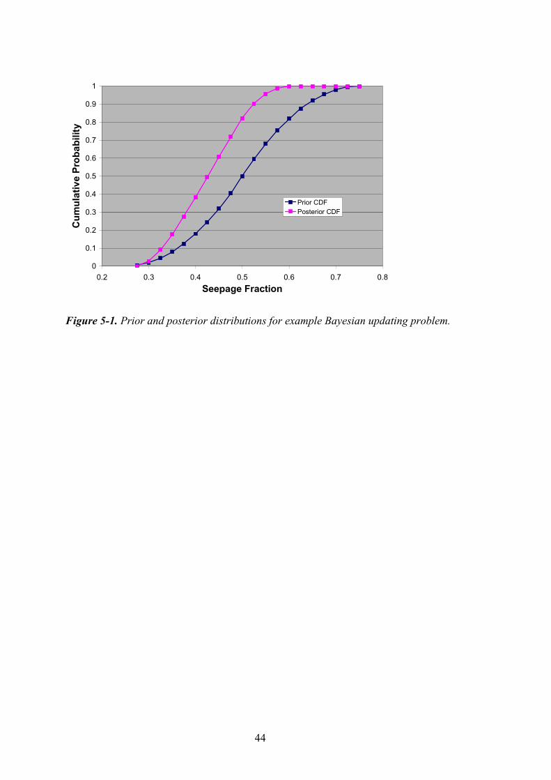
44
0
0.1
0.2
0.3
0.4
0.5
0.6
0.7
0.8
0.9
1
0.2 0.3 0.4 0.5 0.6 0.7 0.8
Seepage Fraction
Cu
mu
lati
ve P
rob
abili
ty
Prior CDFPosterior CDF
Figure 5-1. Prior and posterior distributions for example Bayesian updating problem.
45
6 Concluding remarks
6.1 Summary This white paper provides an overview of various approaches for assigning probability distributions to input parameters of performance assessment models. The report begins with a summary of the nature of data and distributions, followed by a discussion of several common theoretical parametric models for characterizing distributions.
Next, various techniques are presented for fitting continuous distributions to data. These include probability plotting, method of moments, maximum likelihood estimation and nonlinear least squares analysis. The techniques are demonstrated using data from a recent performance assessment study for the Yucca Mountain project. Goodness of fit techniques are also discussed, followed by an overview of how distribution fitting is accomplished in commercial software packages.
The issue of subjective assessment of probabilities is dealt with in terms of the maximum entropy distribution selection approach, as well as some common rules for codifying informal expert judgment. Formal expert elicitation protocols are discussed next, and are based primarily on the guidance provided by the US NRC.
Finally, the Bayesian framework for updating prior distributions (beliefs) when new information becomes available is discussed.
6.2 Recommended process for assigning distributions Based on the material presented thus far, a two-part strategy is recommended for assigning distributions. The first part of the strategy deals with the situation where enough data are available to define an empirical CDF or fit a parametric model to the data, and involves the following step-wise process.
1. Evaluate data for adequacy, and re-sample if necessary.
2. Determine if the data need updating, and apply Bayesian techniques as needed.
3. Construct empirical CDF.
4. Determine if parametric distribution is to be fitted. If not, then pass empirical CDF and skip steps 5–10.
5. Perform probability plotting.
6. Select candidate distributions for fitting. If none are identified, then pass empirical CDF and skip steps 7–10.
7. Estimate distribution parameters.
8. Compute goodness-of-fit statistics.
9. Determine if the fit is acceptable. If not, then pass empirical CDF and stop.
10. Pass selected distribution and fitted parameters.

46
The second part of the strategy deals with the situation where only a limited amount of information is available.
1. If the conditions for a formal expert elicitation exist, then use the protocol described in section 4.3.
2. If historical data and analogs are available, use the maximum entropy approach for selecting a distribution. If not, then develop subjective distributions based on informal expert judgment.
Finally, it should be pointed out that it is not necessary for all inputs in a probabilistic performance model to be characterized as uncertain quantities. The selection of uncertain parameters should be based on observed importance in past analyses, perceived importance with respect to the planned analyses, and the general level of interest in the variable /Helton, 1993/. This facilitates an efficient utilization of resources for developing the uncertainty characterization, implementing the probabilistic calculations and interpreting their results.
47
7 References
Ang A H-S, Tang W H, 1975. Probability Concepts in Engineering Planning and Design, John Wiley and Sons, New York.
Benjamin J R, Cornell C A, 1970. Probability, Statistics and Decisions for Civil Engineers, McGraw-Hill, New York.
Coppersmith K J, Perman R C, Youngs R R, Pendleton M, 1998. “Use of expert elicitation to quantify uncertainties in process models for total system performance assessment,” Proceedings, Eighth International Conference on High-Level Radioactive Waste Management, Las Vegas, May 11–14, p. 318–320.
Cullen A C, Frey H C, 1999. Probabilistic Techniques in Exposure Assessment, Plenum Press, New York.
D’Agostino R B, Stephens M A (eds.), 1986. Goodness-of-Fit Techniques, Marcel Dekker, New York.
DeGroot M H, 1970. Optimal Statistical Decisions, MC-Graw Hill, New York.
Farmer J C, McCright R D, Jones D, Lingenfelter A, Stahl D, 2000. General Corrosion and Localized Corrosion of Waste Package Outer Barrier, Report ANL-EBS-MD-000003 Rev.00, Office of Civilian Radioactive Waste Management, Yucca Mountain Project, Las Vegas.
Frey H C, Burmaster D E, 1999. “Methods for characterizing variability and uncertainty: comparison of bootstrap simulation and likelihood-based approaches,” Risk Analysis, 19:109–130.
Hahn G J, Shapiro S S, 1967. Statistical Models in Engineering, John Wiley and Sons, New York.
Harr M E, 1987. Reliability-Based Design in Civil Engineering, McGraw-Hill, New York.
Hedin A, 2002. “Integrated analytic radionuclide transport model for a spent nuclear fuel repository in saturated fractured rock,” Nuclear Technology, 183 (May, in press).
Helton J C, 1993. “Uncertainty and sensitivity analysis techniques for use in performance assessment for radioactive waste disposal,” Reliability Engineering and System safety, 42:327–367.
Helton J C, Anderson D R (eds.), 1999. Special Collection: Performance Assessment for Radioactive Waste Disposal, Risk Analysis, 19:759–1016.
Hoffmann F O, 1996. “The effect of distribution choice for uncertain parameters in a Monte Carlo analysis,” presented at Society for Risk Analysis Annual Meeting, Workshop on Quantitative Techniques for Analysis of Variability and Uncertainty in Exposure and Risk Assessment, New Orleans, December 8.
Hora S C, Iman R L, 1989. “Expert opinion in risk analysis – the NUREG-1150 methodology,” Nuclear Science and Engineering, 102:323–331.

48
Iman R L, 1980. Risk Methodology for Geologic Disposal of Radioactive Waste: Small Sample Sensitivity Techniques for Computer Models, NUREG CR-1397, SAND 80–1397, Sandia National Laboratories, NM.
Iman R L, Conover W J, 1983. A Modern Approach to Statistics, John Wiley and Sons, New York.
IAEA (International Atomic Energy Agency), 1989. Evaluating the Reliability of Predictions Made Using Environmental Transfer Models, Safety Series, No. 100, Vienna, Austria.
Kotra J P, Lee M P, Eisenberg N A, DeWispelare A R, 1996. Branch Technical Position on the Use of Expert Elicitation in the High-Level Radioactive Waste Program, NUREG-1563, US Nuclear Regulatory Commission.
Kuzio S, 1999. Probability Distributions for Flowing Interval Spacing, Report ANL-NBS-MD-000003 Rev.00, Office of Civilian Radioactive Waste Management, Yucca Mountain Project, Las Vegas.
Lindgren M, Lindstrom F, 1999. SR 97 Radionuclide Transport Calculations, Technical Report TR-99-23, Swedish Nuclear Fuel and Waste Management Company (SKB), Stockholm.
Mattie P D, Miller S P, 2000. Total System Performance Assessment Model for the Site Recommendation, Report MDL-WIS-MD-000002 Rev.00, Office of Civilian Radioactive Waste Management, Yucca Mountain Project, Las Vegas.
Morgan M G, Henrion M, 1990. A Guide to Dealing with Uncertainty in Quantitative Risk and Policy Analysis, Cambridge University Press, New York.
NCRP (National Council on Radiation Protection and Measurements), 1996. Guide for Uncertainty Analysis in Dose and Risk Assessments Related to Environmental Contamination, NCRP Commentary No. 14, Bethesda, MD.
RamaRao B S, Mishra S, McNeish J A, Andrews R W, 2001. “Sensitivity of Monte Carlo simulations to input distributions,” Proceedings, SAMO2001, Third International Symposium on Sensitivity Analysis of Model Output, Madrid, Spain, June 18–20, p. 245–248.
Sauer M L, 2000. Igneous Consequence Modeling for the TSPA-SR, Report ANL-WIS-MD-000017 Rev.00 ICN 01, Office of Civilian Radioactive Waste Management, Yucca Mountain Project, Las Vegas.
Thompson K M, 1999. “Developing univariate distributions from data for risk analysis,” Human and Ecological Risk Assessment, 5:755–783.
US DOE (Department of Energy), 1995. Principles and Guidelines for Formal Use of Expert Judgment by the Yucca Mountain Site Characterization Project, Office of Civilian Radioactive Waste Management, Yucca Mountain Site Characterization Office.
US DOE (Department of Energy), 1998. Total System Performance Assessment. Volume 3 of Viability Assessment of a Repository at Yucca Mountain, DOE/RW-0508, US Department of Energy, Office of Civilian Radioactive Waste Management, Washington, D.C.

49
US EPA (Environmental Protection Agency), 1997. Guiding Principles for Monte Carlo Analysis, EPA/630/R-97/001, Risk Assessment Forum, Washington, D.C.
Venables W N, Ripley B D, 1997. Modern Applied Statistics with S-PLUS, Second Edition, Springer, New York.
Wilson M L, 2000. Abstraction of Drift Seepage, Report ANL-NBS-MD-000005 Rev.01C, Office of Civilian Radioactive Waste Management, Yucca Mountain Project, Las Vegas.

ISSN 1404-0344CM Digitaltryck AB, Bromma, 2002