Embed Size (px)
Citation preview
Assimilation AlgorithmsLecture 1: Basic Concepts
Sébastien Massart and Mike Fisher
ECMWF
24 February 2020
EUROPEAN CENTRE FOR MEDIUM-RANGE WEATHER FORECASTS October 29, 2014
Outline
1 History and Terminology
2 Elementary Statistics — The Scalar Analysis Problem
3 Extension to Multiple Dimensions
4 Optimal Interpolation
5 Summary
c©ECMWF 2 / 38
EUROPEAN CENTRE FOR MEDIUM-RANGE WEATHER FORECASTS October 29, 2014
Outline
1 History and Terminology
2 Elementary Statistics — The Scalar Analysis Problem
3 Extension to Multiple Dimensions
4 Optimal Interpolation
5 Summary
c©ECMWF 3 / 38
EUROPEAN CENTRE FOR MEDIUM-RANGE WEATHER FORECASTS October 29, 2014
Interpreting the weather situation
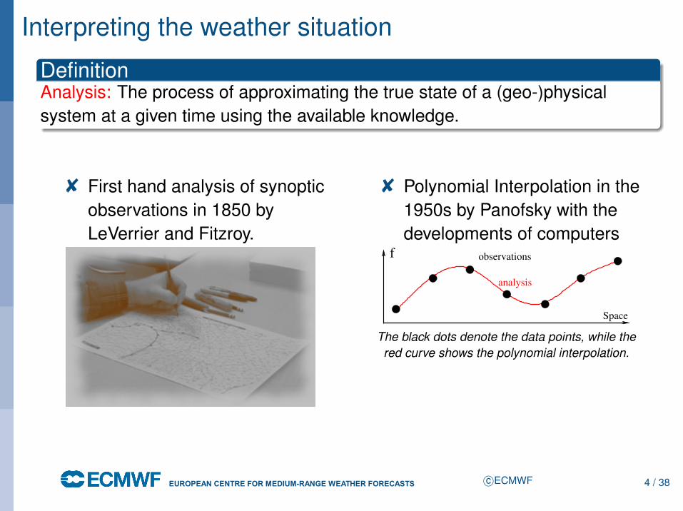
DefinitionAnalysis: The process of approximating the true state of a (geo-)physicalsystem at a given time using the available knowledge.
8 First hand analysis of synopticobservations in 1850 byLeVerrier and Fitzroy.
8 Polynomial Interpolation in the1950s by Panofsky with thedevelopments of computers
f observations
analysis
Space
The black dots denote the data points, while thered curve shows the polynomial interpolation.
c©ECMWF 4 / 38

EUROPEAN CENTRE FOR MEDIUM-RANGE WEATHER FORECASTS October 29, 2014
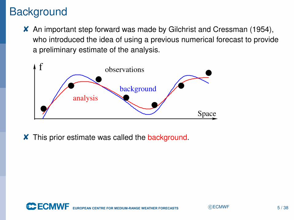
Background8 An important step forward was made by Gilchrist and Cressman (1954),
who introduced the idea of using a previous numerical forecast to providea preliminary estimate of the analysis.
f observations
Space
background
8 This prior estimate was called the background.
c©ECMWF 5 / 38
EUROPEAN CENTRE FOR MEDIUM-RANGE WEATHER FORECASTS October 29, 2014
Background8 An important step forward was made by Gilchrist and Cressman (1954),
who introduced the idea of using a previous numerical forecast to providea preliminary estimate of the analysis.
f observations
Space
background
analysis
8 This prior estimate was called the background.
c©ECMWF 5 / 38
EUROPEAN CENTRE FOR MEDIUM-RANGE WEATHER FORECASTS October 29, 2014
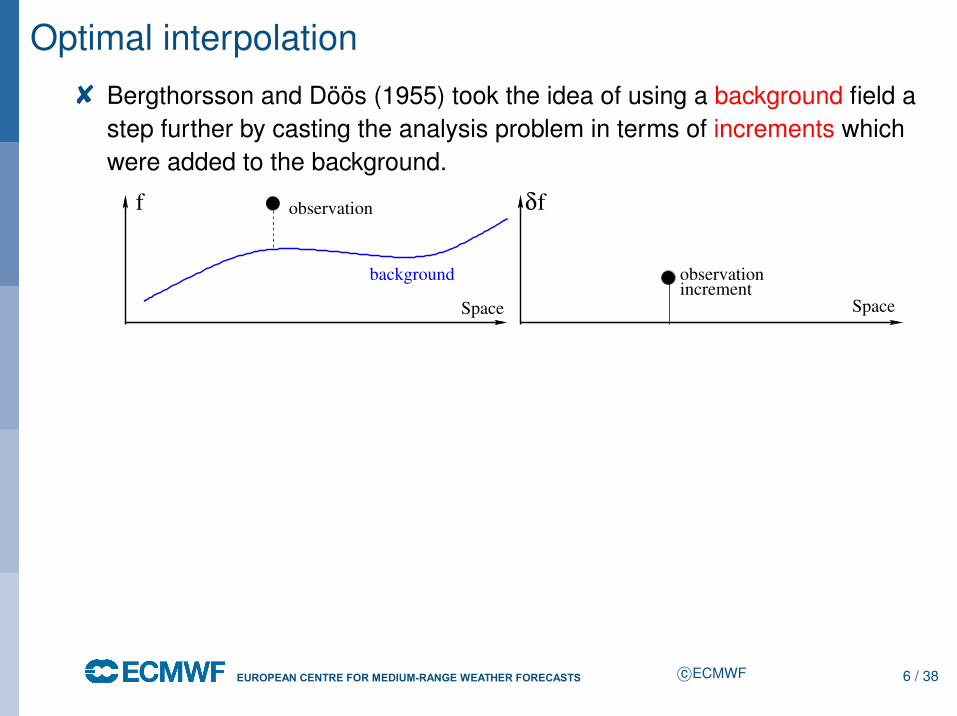
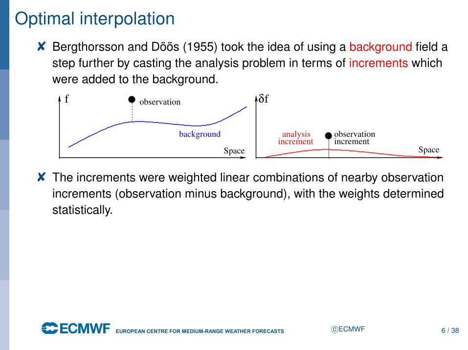
Optimal interpolation8 Bergthorsson and Döös (1955) took the idea of using a background field a
step further by casting the analysis problem in terms of increments whichwere added to the background.
f observation
background
Space
observationincrement
Space
δf
c©ECMWF 6 / 38
EUROPEAN CENTRE FOR MEDIUM-RANGE WEATHER FORECASTS October 29, 2014
Optimal interpolation8 Bergthorsson and Döös (1955) took the idea of using a background field a
step further by casting the analysis problem in terms of increments whichwere added to the background.
f observation
background
Space
observationincrement
Spaceincrementanalysis
δf
8 The increments were weighted linear combinations of nearby observationincrements (observation minus background), with the weights determinedstatistically.
c©ECMWF 6 / 38
EUROPEAN CENTRE FOR MEDIUM-RANGE WEATHER FORECASTS October 29, 2014
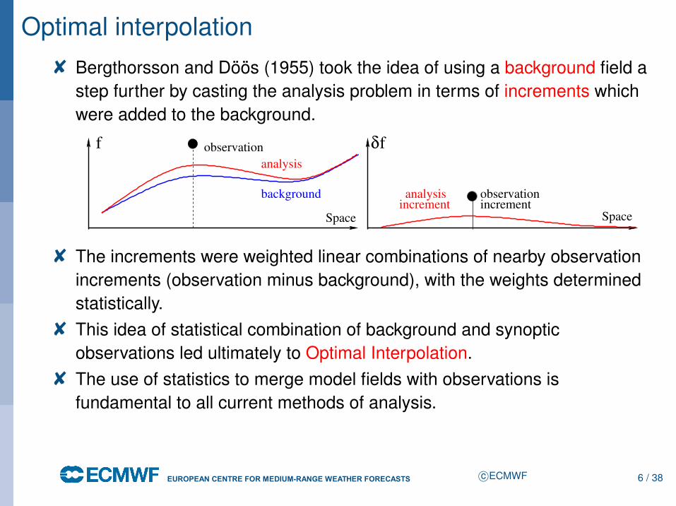
Optimal interpolation8 Bergthorsson and Döös (1955) took the idea of using a background field a
step further by casting the analysis problem in terms of increments whichwere added to the background.
f observation
analysis
background
Space
observationincrement
Spaceincrementanalysis
δf
8 The increments were weighted linear combinations of nearby observationincrements (observation minus background), with the weights determinedstatistically.
8 This idea of statistical combination of background and synopticobservations led ultimately to Optimal Interpolation.
8 The use of statistics to merge model fields with observations isfundamental to all current methods of analysis.
c©ECMWF 6 / 38
EUROPEAN CENTRE FOR MEDIUM-RANGE WEATHER FORECASTS October 29, 2014
Data Assimilation8 An important change of emphasis happened in the early 1970s with the
introduction of primitive-equation models.8 Primitive equation models support inertia-gravity waves. This makes them
much more fussy about their initial conditions than the filtered models thathad been used hitherto.
8 The analysis procedure became much more intimately linked with themodel. The analysis had to produce an initial state that respected themodel’s dynamical balances.
8 Unbalanced increments from the analysis procedure would be rejected asa result of geostrophic adjustment.
8 Initialisation techniques (which suppress inertia-gravity waves) becameimportant.
c©ECMWF 7 / 38
EUROPEAN CENTRE FOR MEDIUM-RANGE WEATHER FORECASTS October 29, 2014
Data AssimilationThe idea that the analysis procedure must present observational information tothe model in a way in which it can be absorbed (i.e. not rejected by geostrophicadjustment) led to the coining of the term data assimilation.
Wiktionary: Assimilate1. To incorporate nutrients into the body, especially after digestion.
ë Food is assimilated and converted into organic tissue.
2. To incorporate or absorb knowledge into the mind.ë The teacher paused in their lecture to allow the students to assimilate what they had said.
3. To absorb a group of people into a community.ë The aliens in the science-fiction film wanted to assimilate human beings into their own race.
c©ECMWF 8 / 38
EUROPEAN CENTRE FOR MEDIUM-RANGE WEATHER FORECASTS October 29, 2014
Data AssimilationThe idea that the analysis procedure must present observational information tothe model in a way in which it can be absorbed (i.e. not rejected by geostrophicadjustment) led to the coining of the term data assimilation.
Wiktionary: Assimilate1. To incorporate nutrients into the body, especially after digestion.
ë Food is assimilated and converted into organic tissue.
2. To incorporate or absorb knowledge into the mind.ë The teacher paused in their lecture to allow the students to assimilate what they had said.
3. To absorb a group of people into a community.ë The aliens in the science-fiction film wanted to assimilate human beings into their own race.
ë The process by which the Borg integrate beings and cultures into their collective.
Our definition8 The process of objectively adapting the model state to observations in a
statistically optimal way taking into account model and observation errors
c©ECMWF 8 / 38
EUROPEAN CENTRE FOR MEDIUM-RANGE WEATHER FORECASTS October 29, 2014
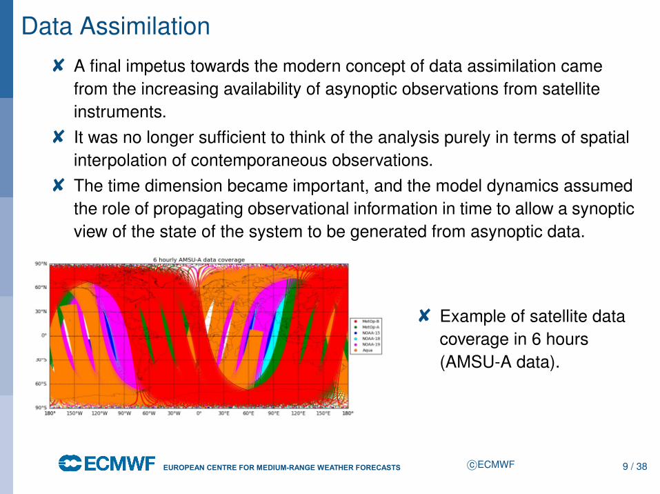
Data Assimilation8 A final impetus towards the modern concept of data assimilation came
from the increasing availability of asynoptic observations from satelliteinstruments.
8 It was no longer sufficient to think of the analysis purely in terms of spatialinterpolation of contemporaneous observations.
8 The time dimension became important, and the model dynamics assumedthe role of propagating observational information in time to allow a synopticview of the state of the system to be generated from asynoptic data.
8 Example of satellite datacoverage in 6 hours(AMSU-A data).
c©ECMWF 9 / 38
EUROPEAN CENTRE FOR MEDIUM-RANGE WEATHER FORECASTS October 29, 2014
Outline
1 History and Terminology
2 Elementary Statistics — The Scalar Analysis Problem
3 Extension to Multiple Dimensions
4 Optimal Interpolation
5 Summary
c©ECMWF 10 / 38
EUROPEAN CENTRE FOR MEDIUM-RANGE WEATHER FORECASTS October 29, 2014
Elementary StatisticsProblemSuppose we want to estimate the temperature of this room, given:
8 A prior estimate: Tb.ë E.g., room thermostat or assume we measured the temperature an hour ago, and
we have some idea (i.e. a model) of how the temperature varies as a function oftime, the number of people in the room, whether the windows are open, etc.
8 A thermometer: To.8 Denote the true temperature of the room by Tt .
Errors8 The errors in Tb and To are:
εb = Tb−Tt
εo = To−Tt
8 εb and εo are random variables (or stochastic variables)
c©ECMWF 11 / 38
EUROPEAN CENTRE FOR MEDIUM-RANGE WEATHER FORECASTS October 29, 2014
Elementary StatisticsHypotheses
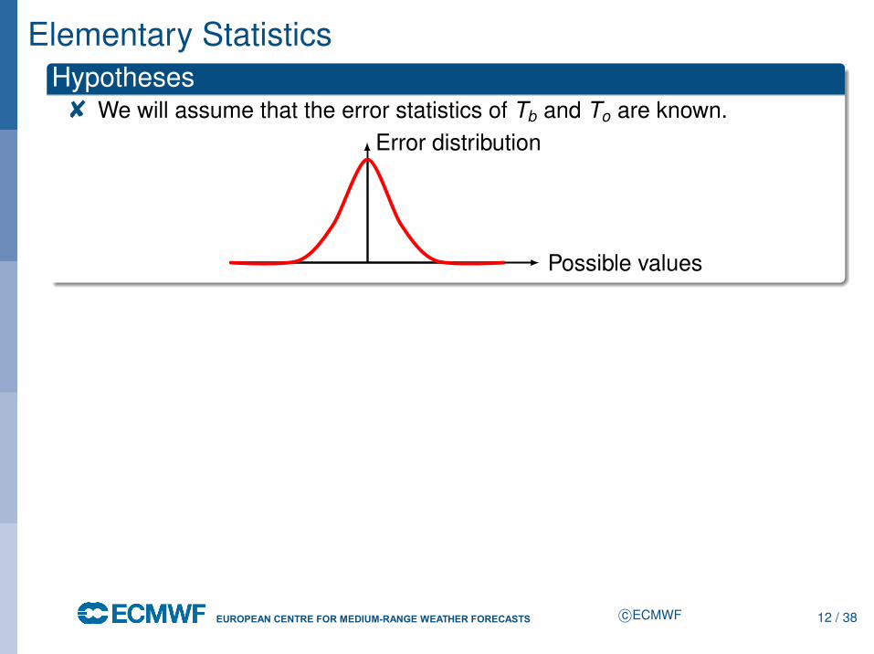
8 We will assume that the error statistics of Tb and To are known.
Possible values
Error distribution
c©ECMWF 12 / 38
EUROPEAN CENTRE FOR MEDIUM-RANGE WEATHER FORECASTS October 29, 2014
Elementary StatisticsHypotheses
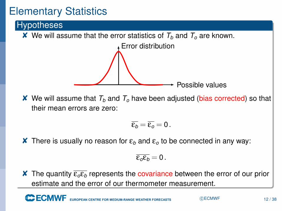
8 We will assume that the error statistics of Tb and To are known.
Possible values
Error distribution
8 We will assume that Tb and To have been adjusted (bias corrected) so thattheir mean errors are zero:
εb = εo = 0 .
8 There is usually no reason for εb and εo to be connected in any way:
εoεb = 0 .
8 The quantity εoεb represents the covariance between the error of our priorestimate and the error of our thermometer measurement.
c©ECMWF 12 / 38
EUROPEAN CENTRE FOR MEDIUM-RANGE WEATHER FORECASTS October 29, 2014
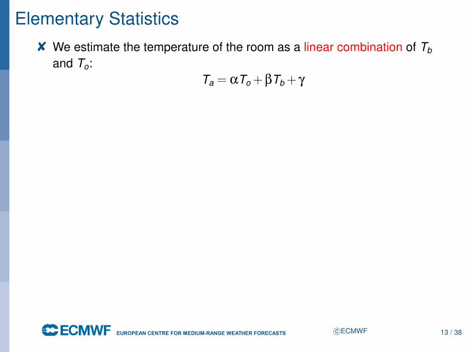
Elementary Statistics8 We estimate the temperature of the room as a linear combination of Tb
and To:Ta = αTo +βTb + γ
c©ECMWF 13 / 38
EUROPEAN CENTRE FOR MEDIUM-RANGE WEATHER FORECASTS October 29, 2014
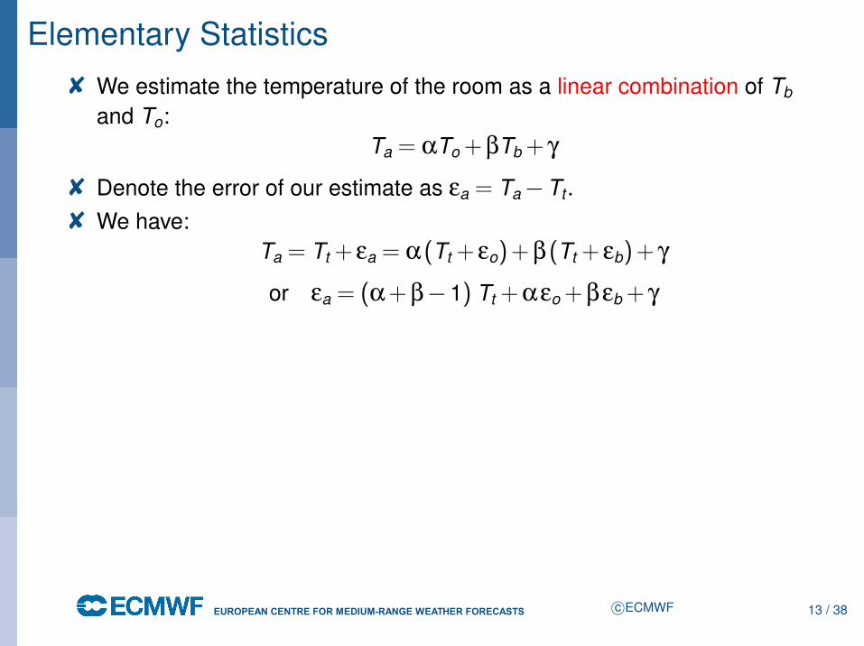
Elementary Statistics8 We estimate the temperature of the room as a linear combination of Tb
and To:Ta = αTo +βTb + γ
8 Denote the error of our estimate as εa = Ta−Tt .8 We have:
Ta = Tt + εa = α (Tt + εo)+β (Tt + εb)+ γ
or εa = (α+β−1) Tt +αεo +βεb + γ
c©ECMWF 13 / 38
EUROPEAN CENTRE FOR MEDIUM-RANGE WEATHER FORECASTS October 29, 2014
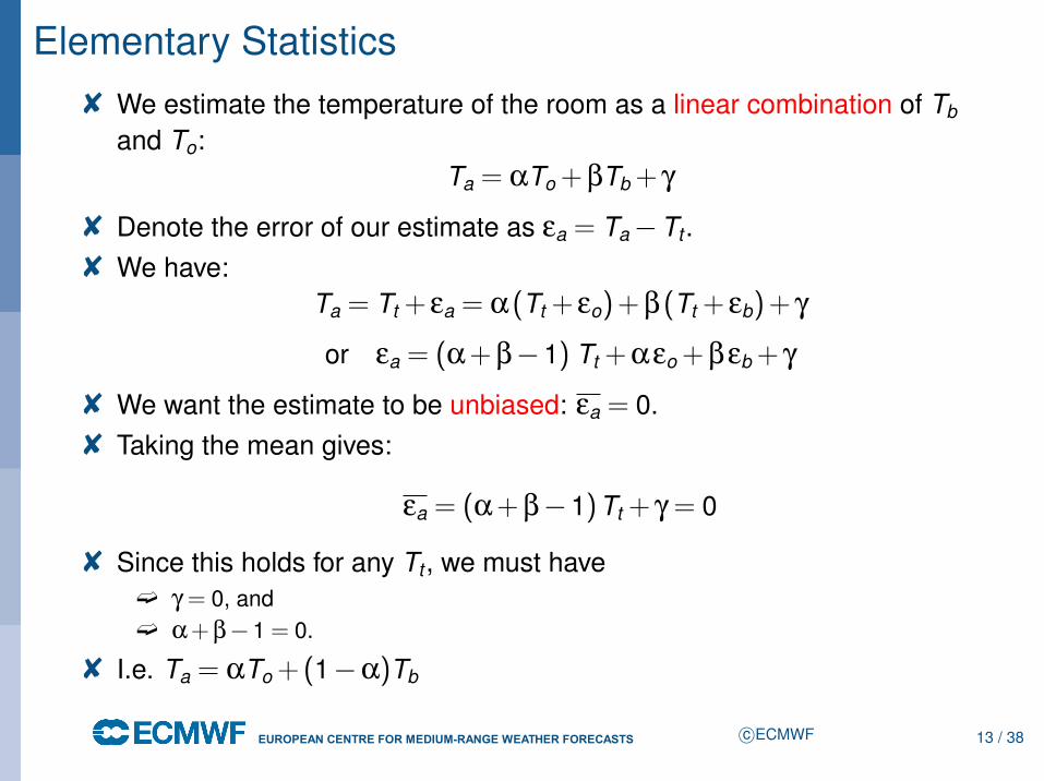
Elementary Statistics8 We estimate the temperature of the room as a linear combination of Tb
and To:Ta = αTo +βTb + γ
8 Denote the error of our estimate as εa = Ta−Tt .8 We have:
Ta = Tt + εa = α (Tt + εo)+β (Tt + εb)+ γ
or εa = (α+β−1) Tt +αεo +βεb + γ
8 We want the estimate to be unbiased: εa = 0.8 Taking the mean gives:
εa = (α+β−1)Tt + γ = 0
8 Since this holds for any Tt , we must haveë γ = 0, andë α+β−1 = 0.
8 I.e. Ta = αTo +(1−α)Tb
c©ECMWF 13 / 38

EUROPEAN CENTRE FOR MEDIUM-RANGE WEATHER FORECASTS October 29, 2014
Elementary Statistics8 The general Linear Unbiased Estimate is:
Ta = αTo +(1−α)Tb
8 Now consider the error of this estimate.8 Subtracting Tt from both sides of the equation gives
εa = αεo +(1−α)εb
c©ECMWF 14 / 38
EUROPEAN CENTRE FOR MEDIUM-RANGE WEATHER FORECASTS October 29, 2014
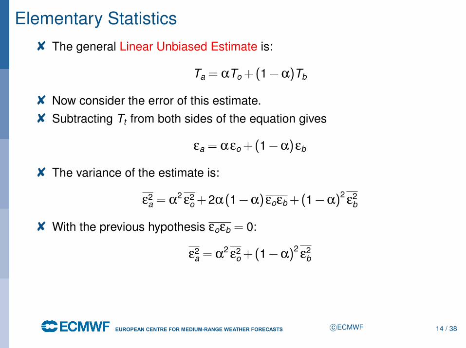
Elementary Statistics8 The general Linear Unbiased Estimate is:
Ta = αTo +(1−α)Tb
8 Now consider the error of this estimate.8 Subtracting Tt from both sides of the equation gives
εa = αεo +(1−α)εb
8 The variance of the estimate is:
ε2a = α
2ε2
o +2α (1−α)εoεb +(1−α)2ε2
b
8 With the previous hypothesis εoεb = 0:
ε2a = α
2ε2
o +(1−α)2ε2
b
c©ECMWF 14 / 38
EUROPEAN CENTRE FOR MEDIUM-RANGE WEATHER FORECASTS October 29, 2014
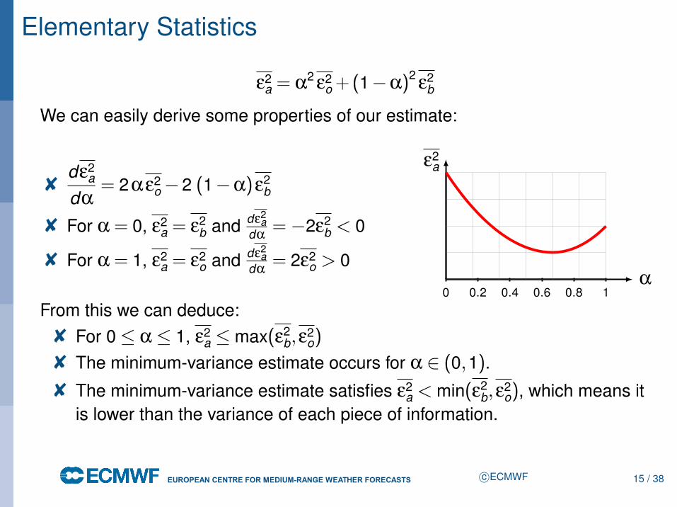
Elementary Statistics
ε2a = α
2ε2
o +(1−α)2ε2
b
We can easily derive some properties of our estimate:
8dε2
a
dα= 2αε2
o−2 (1−α)ε2b
8 For α = 0, ε2a = ε2
b and dε2a
dα=−2ε2
b < 0
8 For α = 1, ε2a = ε2
o and dε2a
dα= 2ε2
o > 0α
0 0.2 0.4 0.6 0.8 1
ε2a
From this we can deduce:8 For 0≤ α≤ 1, ε2
a ≤max(ε2b,ε
2o)
8 The minimum-variance estimate occurs for α ∈ (0,1).
8 The minimum-variance estimate satisfies ε2a < min(ε2
b,ε2o), which means it
is lower than the variance of each piece of information.
c©ECMWF 15 / 38
EUROPEAN CENTRE FOR MEDIUM-RANGE WEATHER FORECASTS October 29, 2014
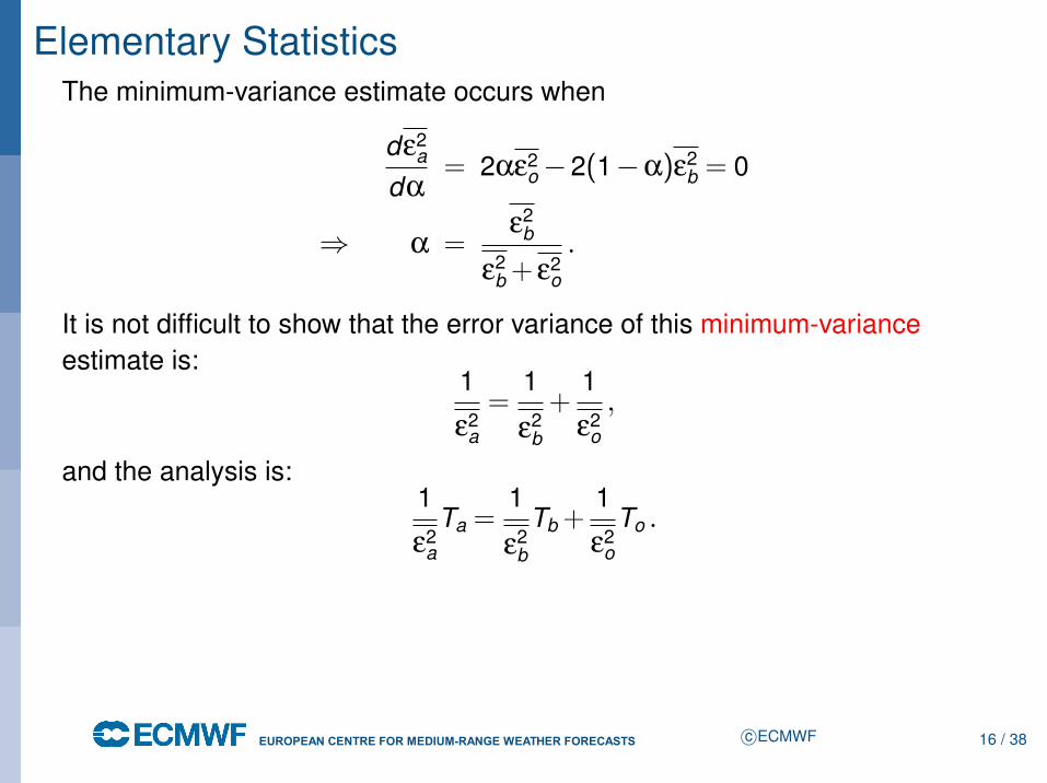
Elementary StatisticsThe minimum-variance estimate occurs when
dε2a
dα= 2αε2
o−2(1−α)ε2b = 0
⇒ α =ε2
b
ε2b + ε2
o
.
It is not difficult to show that the error variance of this minimum-varianceestimate is:
1
ε2a
=1
ε2b
+1
ε2o
,
and the analysis is:1
ε2a
Ta =1
ε2b
Tb +1
ε2o
To .
c©ECMWF 16 / 38
EUROPEAN CENTRE FOR MEDIUM-RANGE WEATHER FORECASTS October 29, 2014
Outline
1 History and Terminology
2 Elementary Statistics — The Scalar Analysis Problem
3 Extension to Multiple Dimensions
4 Optimal Interpolation
5 Summary
c©ECMWF 17 / 38
EUROPEAN CENTRE FOR MEDIUM-RANGE WEATHER FORECASTS October 29, 2014
Extension to Multiple Dimensions8 Now, let’s turn our attention to the multi-dimensional case.8 Instead of a scalar prior estimate Tb, we now consider a vector xb.8 We can think of xb as representing the entire state of a numerical model at
some time.8 The elements of xb might be grid-point values, spherical harmonic
coefficients, etc., and some elements may represent temperatures,humidity, others wind components, etc.
8 We refer to xb as the background.8 Similarly, we generalise the observation to a vector y.8 y can contain a disparate collection of observations at different locations,
and of different variables.
c©ECMWF 18 / 38
EUROPEAN CENTRE FOR MEDIUM-RANGE WEATHER FORECASTS October 29, 2014
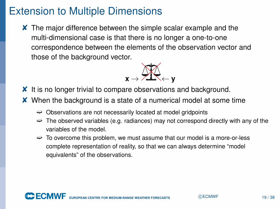
Extension to Multiple Dimensions8 The major difference between the simple scalar example and the
multi-dimensional case is that there is no longer a one-to-onecorrespondence between the elements of the observation vector andthose of the background vector.
x→ ← y8 It is no longer trivial to compare observations and background.8 When the background is a state of a numerical model at some time
ë Observations are not necessarily located at model gridpointsë The observed variables (e.g. radiances) may not correspond directly with any of the
variables of the model.ë To overcome this problem, we must assume that our model is a more-or-less
complete representation of reality, so that we can always determine “modelequivalents” of the observations.
c©ECMWF 19 / 38
EUROPEAN CENTRE FOR MEDIUM-RANGE WEATHER FORECASTS October 29, 2014
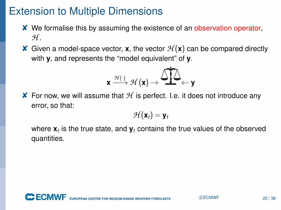
Extension to Multiple Dimensions8 We formalise this by assuming the existence of an observation operator,
H .8 Given a model-space vector, x, the vector H (x) can be compared directly
with y, and represents the “model equivalent” of y.
xH (·)−−→H (x)→ ← y
8 For now, we will assume that H is perfect. I.e. it does not introduce anyerror, so that:
H (xt) = yt
where xt is the true state, and yt contains the true values of the observedquantities.
c©ECMWF 20 / 38
EUROPEAN CENTRE FOR MEDIUM-RANGE WEATHER FORECASTS October 29, 2014
Extension to Multiple Dimensions8 As we did in the scalar case, we will look for an analysis that is a linear
combination of the available information:
xa = Fxb +Ky+c
where F and K are matrices, and where c is a vector.8 If H is linear, we can proceed as in the scalar case and look for a linear
unbiased estimate.8 In the more general case of nonlinear H , we will require that error-free
inputs (xb = xt and y = yt) produce an error-free analysis (xa = xt):
xt = Fxt +KH (xt)+c
8 Since this applies for any xt , we must have c = 0 and
I≡ F+KH (·) or F≡ I−KH (·)
8 Our analysis equation is thus:
xa = xb +K (y−H (xb))c©ECMWF 21 / 38
EUROPEAN CENTRE FOR MEDIUM-RANGE WEATHER FORECASTS October 29, 2014
Extension to Multiple Dimensions
xa = xb +K (y−H (xb))
8 Remember that in the scalar case, we had
Ta = αTo +(1−α)Tb
= Tb +α(To−Tb)
8 We see that the matrix K plays a role equivalent to that of the coefficient α.8 K is called the gain matrix.8 It determines the weight given to the innovation y−H (xb)8 It handles the transformation of information defined in “observation space”
to the space of model variables.
c©ECMWF 22 / 38
EUROPEAN CENTRE FOR MEDIUM-RANGE WEATHER FORECASTS October 29, 2014
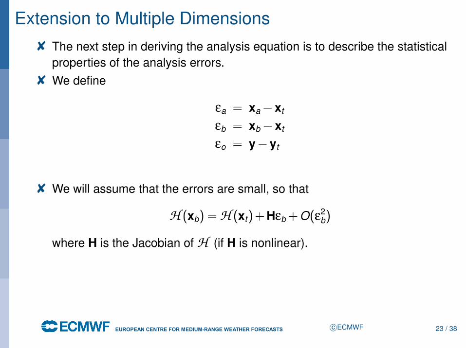
Extension to Multiple Dimensions8 The next step in deriving the analysis equation is to describe the statistical
properties of the analysis errors.8 We define
εa = xa−xt
εb = xb−xt
εo = y−yt
8 We will assume that the errors are small, so that
H (xb) = H (xt)+Hεb +O(ε2b)
where H is the Jacobian of H (if H is nonlinear).
c©ECMWF 23 / 38
EUROPEAN CENTRE FOR MEDIUM-RANGE WEATHER FORECASTS October 29, 2014
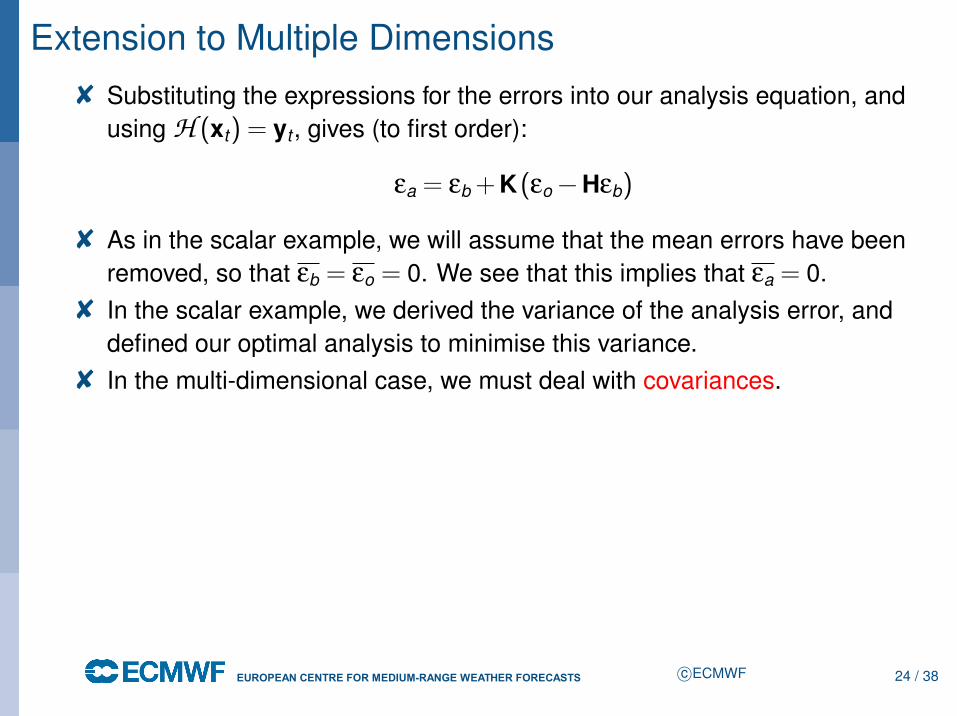
Extension to Multiple Dimensions8 Substituting the expressions for the errors into our analysis equation, and
using H (xt) = yt , gives (to first order):
εa = εb +K (εo−Hεb)
8 As in the scalar example, we will assume that the mean errors have beenremoved, so that εb = εo = 0. We see that this implies that εa = 0.
8 In the scalar example, we derived the variance of the analysis error, anddefined our optimal analysis to minimise this variance.
8 In the multi-dimensional case, we must deal with covariances.
c©ECMWF 24 / 38
EUROPEAN CENTRE FOR MEDIUM-RANGE WEATHER FORECASTS October 29, 2014
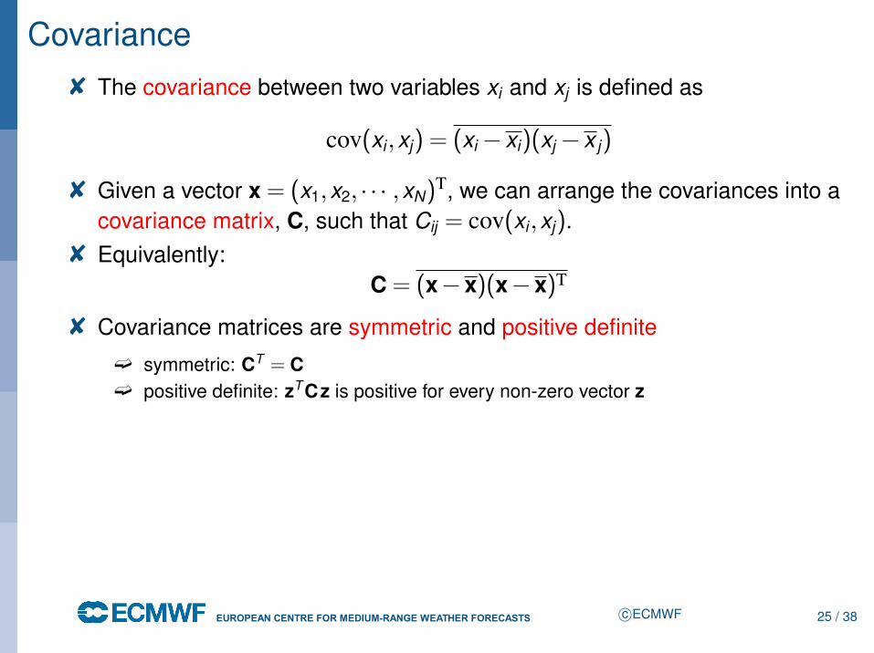
Covariance8 The covariance between two variables xi and xj is defined as
cov(xi,xj) = (xi− xi)(xj− x j)
8 Given a vector x = (x1,x2, · · · ,xN)T, we can arrange the covariances into a
covariance matrix, C, such that Cij = cov(xi,xj).8 Equivalently:
C = (x−x)(x−x)T
8 Covariance matrices are symmetric and positive definite
ë symmetric: CT = Cë positive definite: zT Cz is positive for every non-zero vector z
c©ECMWF 25 / 38
EUROPEAN CENTRE FOR MEDIUM-RANGE WEATHER FORECASTS October 29, 2014
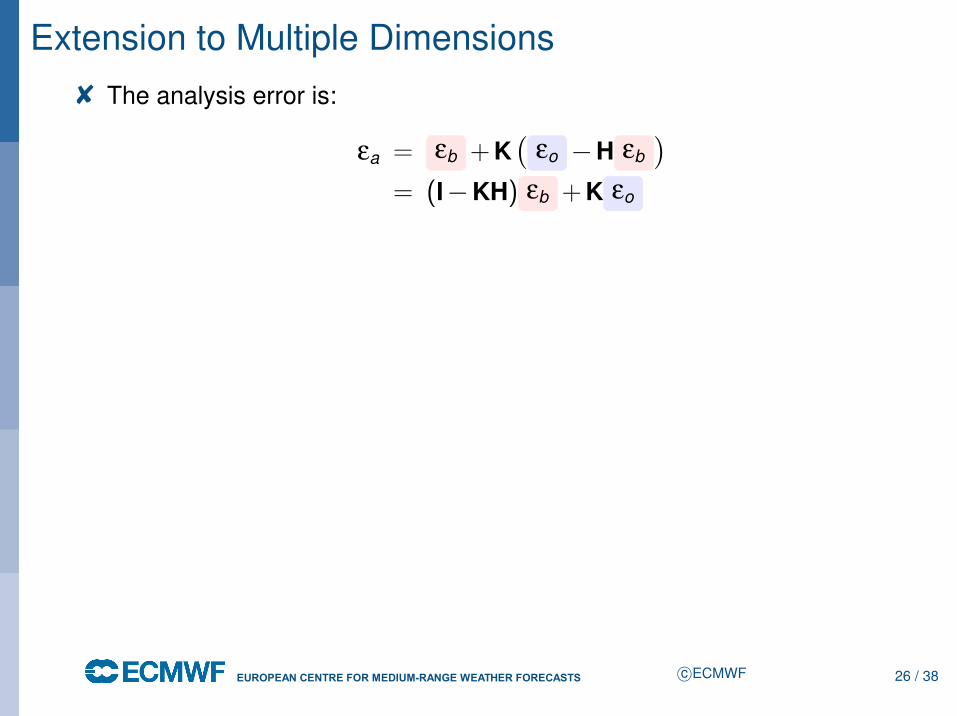
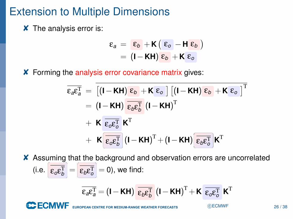
Extension to Multiple Dimensions8 The analysis error is:
εa = εb +K(
εo −H εb)
= (I−KH) εb +K εo
c©ECMWF 26 / 38
EUROPEAN CENTRE FOR MEDIUM-RANGE WEATHER FORECASTS October 29, 2014
Extension to Multiple Dimensions8 The analysis error is:
εa = εb +K(
εo −H εb)
= (I−KH) εb +K εo
8 Forming the analysis error covariance matrix gives:
εaεTa =
[(I−KH) εb +K εo
][(I−KH) εb +K εo
]T
= (I−KH) εbεTb(I−KH)T
+ K εoεTo KT
+ K εoεTb(I−KH)T+(I−KH) εbεT
o KT
8 Assuming that the background and observation errors are uncorrelated
(i.e. εoεTb= εbεT
o = 0), we find:
εaεTa = (I−KH) εbεT
b(I−KH)T+K εoεT
o KT
c©ECMWF 26 / 38
EUROPEAN CENTRE FOR MEDIUM-RANGE WEATHER FORECASTS October 29, 2014
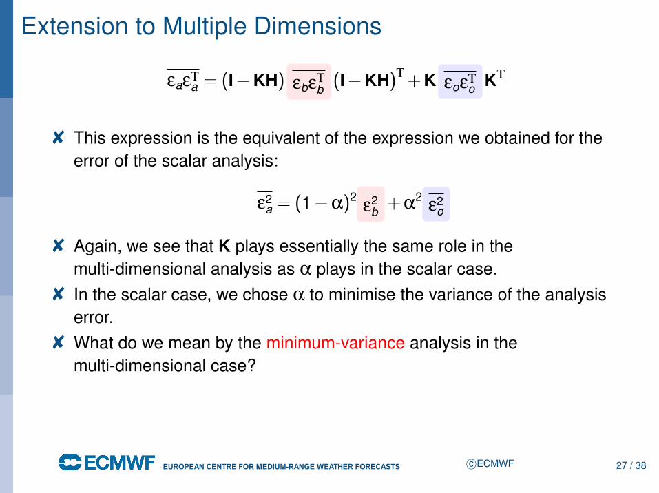
Extension to Multiple Dimensions
εaεTa = (I−KH) εbεT
b(I−KH)T+K εoεT
o KT
8 This expression is the equivalent of the expression we obtained for theerror of the scalar analysis:
ε2a = (1−α)2
ε2b +α
2ε2
o
8 Again, we see that K plays essentially the same role in themulti-dimensional analysis as α plays in the scalar case.
8 In the scalar case, we chose α to minimise the variance of the analysiserror.
8 What do we mean by the minimum-variance analysis in themulti-dimensional case?
c©ECMWF 27 / 38

EUROPEAN CENTRE FOR MEDIUM-RANGE WEATHER FORECASTS October 29, 2014
Extension to Multiple Dimensions8 Note that the diagonal elements of a covariance matrix are variances
Cii = cov(xi,xi) = (xi− xi)2.8 Hence, we can define the minimum-variance analysis as the analysis that
minimises the sum of the diagonal elements of the analysis errorcovariance matrix.
8 The sum of the diagonal elements of a matrix is called the trace.
8 In the scalar case, we found the minimum-variance analysis by setting dε2a
dα
to zero.8 In the multidimensional case, we are going to set
∂trace(εaεTa)
∂K= 0
8 Note:∂trace(εaεT
a)
∂Kis the matrix whose ij th element is
∂trace(εaεTa)
∂Kij.
c©ECMWF 28 / 38
EUROPEAN CENTRE FOR MEDIUM-RANGE WEATHER FORECASTS October 29, 2014
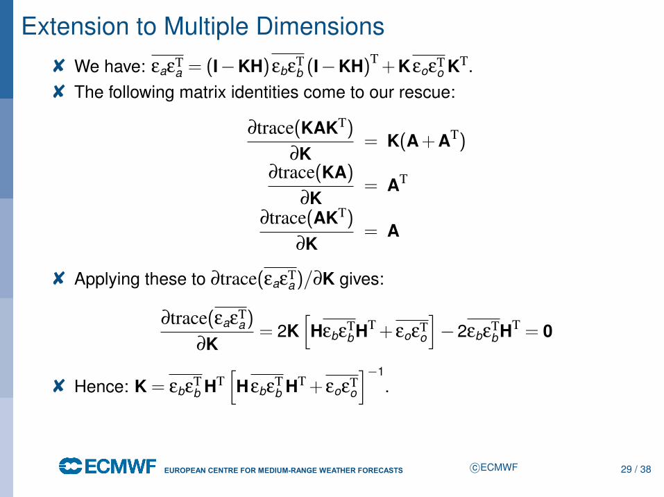
Extension to Multiple Dimensions8 We have: εaεT
a = (I−KH)εbεTb (I−KH)T+KεoεT
o KT.8 The following matrix identities come to our rescue:
∂trace(KAKT)
∂K= K(A+AT)
∂trace(KA)∂K
= AT
∂trace(AKT)
∂K= A
8 Applying these to ∂trace(εaεTa)/∂K gives:
∂trace(εaεTa)
∂K= 2K
[HεbεT
bHT+ εoεTo
]−2εbεT
bHT = 0
8 Hence: K = εbεTb HT
[HεbεT
b HT+ εoεTo
]−1.
c©ECMWF 29 / 38
EUROPEAN CENTRE FOR MEDIUM-RANGE WEATHER FORECASTS October 29, 2014
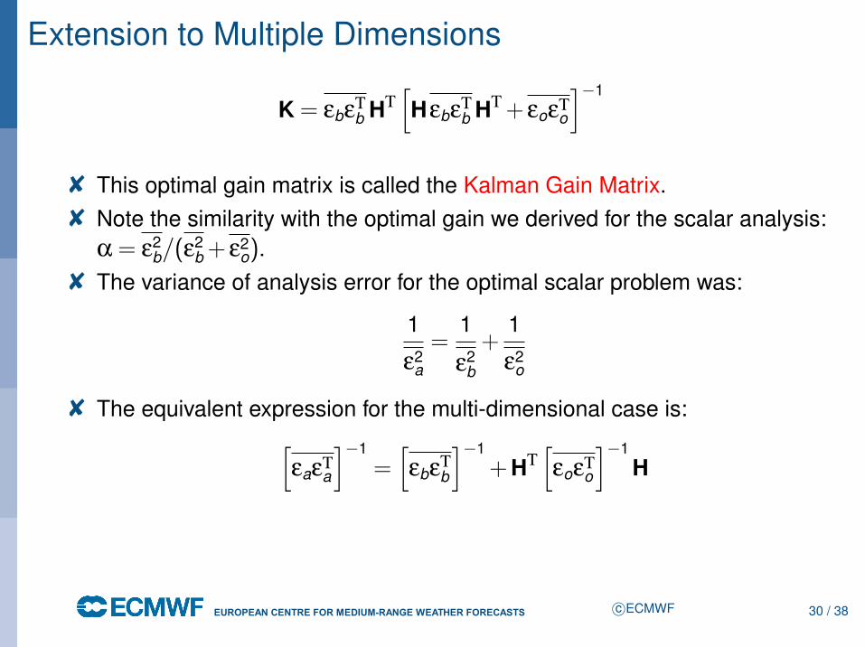
Extension to Multiple Dimensions
K = εbεTb HT
[HεbεT
b HT+ εoεTo
]−1
8 This optimal gain matrix is called the Kalman Gain Matrix.8 Note the similarity with the optimal gain we derived for the scalar analysis:
α = ε2b/(ε
2b + ε2
o).8 The variance of analysis error for the optimal scalar problem was:
1
ε2a
=1
ε2b
+1
ε2o
8 The equivalent expression for the multi-dimensional case is:[εaεT
a
]−1=[εbεT
b
]−1+HT
[εoεT
o
]−1H
c©ECMWF 30 / 38
EUROPEAN CENTRE FOR MEDIUM-RANGE WEATHER FORECASTS October 29, 2014
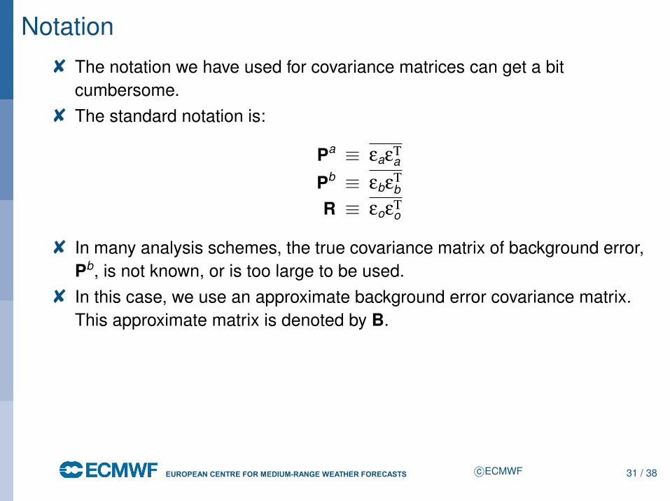
Notation8 The notation we have used for covariance matrices can get a bit
cumbersome.8 The standard notation is:
Pa ≡ εaεTa
Pb ≡ εbεTb
R ≡ εoεTo
8 In many analysis schemes, the true covariance matrix of background error,Pb, is not known, or is too large to be used.
8 In this case, we use an approximate background error covariance matrix.This approximate matrix is denoted by B.
c©ECMWF 31 / 38
EUROPEAN CENTRE FOR MEDIUM-RANGE WEATHER FORECASTS October 29, 2014
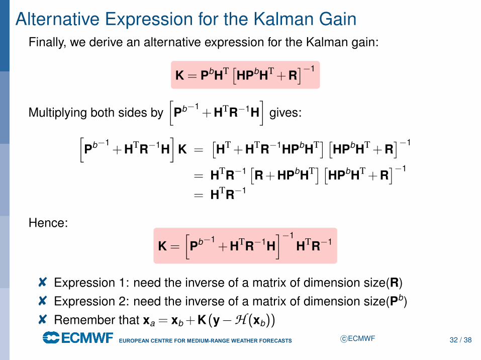
Alternative Expression for the Kalman GainFinally, we derive an alternative expression for the Kalman gain:
K = PbHT [HPbHT+R]−1
Multiplying both sides by[Pb−1
+HTR−1H]
gives:[Pb−1
+HTR−1H]
K =[HT+HTR−1HPbHT][HPbHT+R
]−1
= HTR−1[R+HPbHT][HPbHT+R
]−1
= HTR−1
Hence:
K =[Pb−1
+HTR−1H]−1
HTR−1
8 Expression 1: need the inverse of a matrix of dimension size(R)8 Expression 2: need the inverse of a matrix of dimension size(Pb)8 Remember that xa = xb +K (y−H (xb))
c©ECMWF 32 / 38
EUROPEAN CENTRE FOR MEDIUM-RANGE WEATHER FORECASTS October 29, 2014
Outline
1 History and Terminology
2 Elementary Statistics — The Scalar Analysis Problem
3 Extension to Multiple Dimensions
4 Optimal Interpolation
5 Summary
c©ECMWF 33 / 38
EUROPEAN CENTRE FOR MEDIUM-RANGE WEATHER FORECASTS October 29, 2014
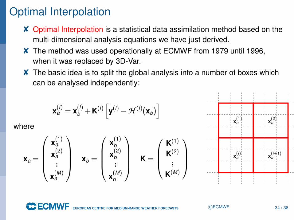
Optimal Interpolation8 Optimal Interpolation is a statistical data assimilation method based on the
multi-dimensional analysis equations we have just derived.8 The method was used operationally at ECMWF from 1979 until 1996,
when it was replaced by 3D-Var.8 The basic idea is to split the global analysis into a number of boxes which
can be analysed independently:
x(i)a = x(i)
b +K(i)[y(i)−H (i)(xb)
]where
xa =
x(1)
a
x(2)a...
x(M)a
xb =
x(1)
b
x(2)b...
x(M)b
K =
K(1)
K(2)
...K(M)
x(1)a x(2)a
x(i)a x(i+1)a
c©ECMWF 34 / 38
EUROPEAN CENTRE FOR MEDIUM-RANGE WEATHER FORECASTS October 29, 2014
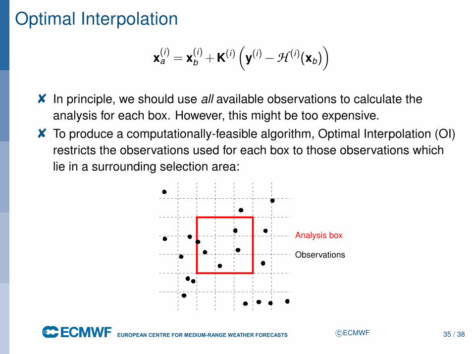
Optimal Interpolation
x(i)a = x(i)
b +K(i)(
y(i)−H (i)(xb))
8 In principle, we should use all available observations to calculate theanalysis for each box. However, this might be too expensive.
8 To produce a computationally-feasible algorithm, Optimal Interpolation (OI)restricts the observations used for each box to those observations whichlie in a surrounding selection area:
Analysis box
Observations
c©ECMWF 35 / 38
EUROPEAN CENTRE FOR MEDIUM-RANGE WEATHER FORECASTS October 29, 2014
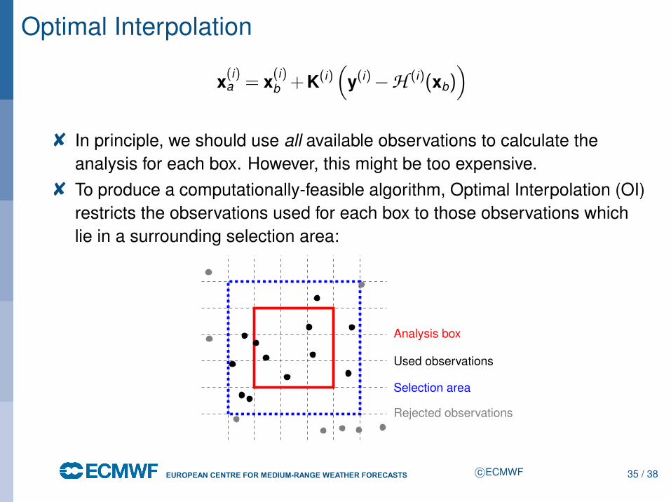
Optimal Interpolation
x(i)a = x(i)
b +K(i)(
y(i)−H (i)(xb))
8 In principle, we should use all available observations to calculate theanalysis for each box. However, this might be too expensive.
8 To produce a computationally-feasible algorithm, Optimal Interpolation (OI)restricts the observations used for each box to those observations whichlie in a surrounding selection area:
Analysis box
Selection area
Used observations
Rejected observations
c©ECMWF 35 / 38
EUROPEAN CENTRE FOR MEDIUM-RANGE WEATHER FORECASTS October 29, 2014
Optimal Interpolation8 The gain matrix used for each box is:
K(i) =(PbHT)(i)[(HPbHT)(i)+R(i)
]−1
8 Now, the dimension of the matrix[(
HPbHT)(i)
+R(i)]
is equal to thenumber of observations in the selection box.
8 Selecting observations reduces the size of this matrix, making it feasible touse direct solution methods to invert it.
8 Note that to implement Optimal Interpolation, we have to specify(PbHT
)(i)and
(HPbHT
)(i). This effectively limits us to very simple observation
operators, corresponding to simple interpolations.8 This, together with the artifacts introduced by observation selection, was
one of the main reasons for abandoning Optimal Interpolation in favour of3D-Var.
c©ECMWF 36 / 38
EUROPEAN CENTRE FOR MEDIUM-RANGE WEATHER FORECASTS October 29, 2014
Outline
1 History and Terminology
2 Elementary Statistics — The Scalar Analysis Problem
3 Extension to Multiple Dimensions
4 Optimal Interpolation
5 Summary
c©ECMWF 37 / 38
EUROPEAN CENTRE FOR MEDIUM-RANGE WEATHER FORECASTS October 29, 2014
Summary8 We derived the linear analysis equation for a simple scalar example.8 We showed that a particular choice of the weight α given to the
observation resulted in an optimal minimum-variance analysis.8 We repeated the derivation for the multi-dimensional case. This required
the introduction of the observation operator.8 The derivation for the multi-dimensional case closely parallelled the scalar
derivation.8 The expressions for the gain matrix and analysis error covariance matrix
were recognisably similar to the corresponding scalar expressions.8 Finally, we considered the practical implementation of the analysis
equation, in an Optimal Interpolation data assimilation scheme.
c©ECMWF 38 / 38