Embed Size (px)
Citation preview
Association Mapping by Local Genealogies
Bioinformatics Research Center
University of Aarhus
http://www.birc.au.dk/[email protected]
Thomas Mailund
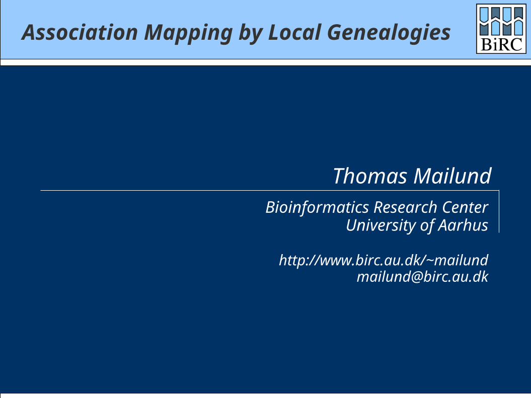
Disease mapping...
--A--------C--------A----G---X----T---C---A------T--------G--------A----G---X----C---C---A------A--------G--------G----G---X----C---C---A------A--------C--------A----G---X----T---C---A------T--------C--------A----G---X----T---C---A------T--------C--------A----T---X----T---A---A----
--A--------C--------A----G---X----T---C---A------A--------C--------A----G---X----T---C---A------A--------C--------A----G---X----T---C---G------T--------C--------A----T---X----T---C---A------A--------C--------A----G---X----T---C---A------A--------C--------G----T---X----C---A---A------A--------C--------A----G---X----C---C---G----
Locate disease locus Unlikely to be among our genotyped markers Use information from available markers
Cases (affected)
Controls (unaffected)
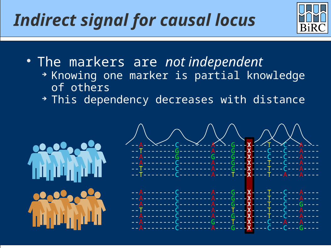
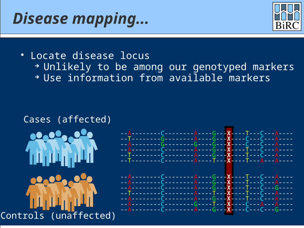
Indirect signal for causal locus
--T--------G--------A----G---X----C---C---A------A--------G--------G----G---X----C---C---A------A--------C--------A----G---X----T---C---A------T--------C--------A----G---X----T---C---A------T--------C--------A----T---X----T---A---A----
--A--------C--------A----G---X----T---C---A------A--------C--------A----G---X----T---C---A------A--------C--------A----G---X----T---C---G------T--------C--------A----T---X----T---C---A------A--------C--------A----G---X----T---C---A------A--------C--------G----T---X----C---A---A------A--------C--------A----G---X----C---C---G----
The markers are not independent Knowing one marker is partial knowledge of others This dependency decreases with distance
--A--------C--------A----G---X----T---C---A----
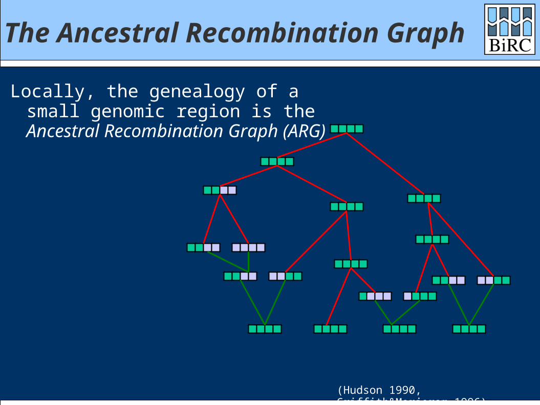
The Ancestral Recombination Graph
Locally, the genealogy of a small genomic region is the Ancestral Recombination Graph (ARG)
(Hudson 1990, Griffith&Marjoram 1996)
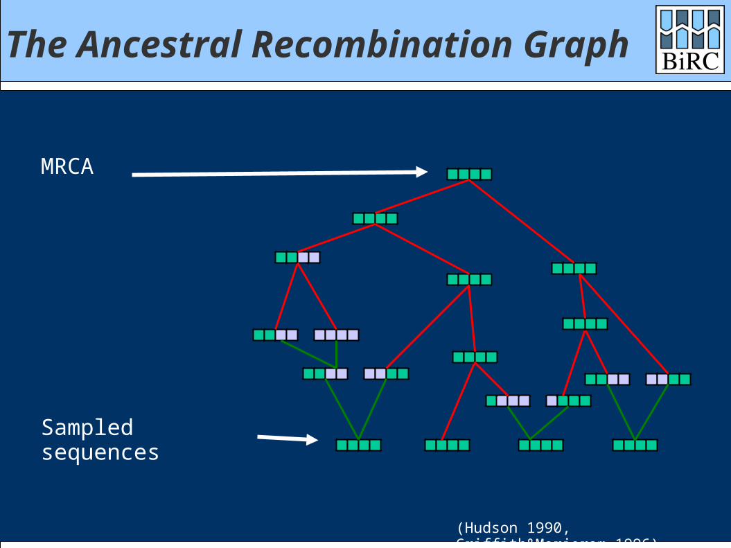
The Ancestral Recombination Graph
Sampled sequences
MRCA
(Hudson 1990, Griffith&Marjoram 1996)
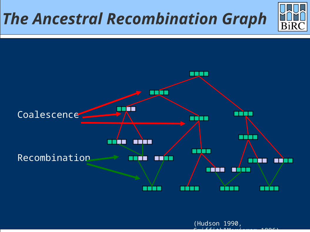
The Ancestral Recombination Graph
Recombination
Coalescence
(Hudson 1990, Griffith&Marjoram 1996)
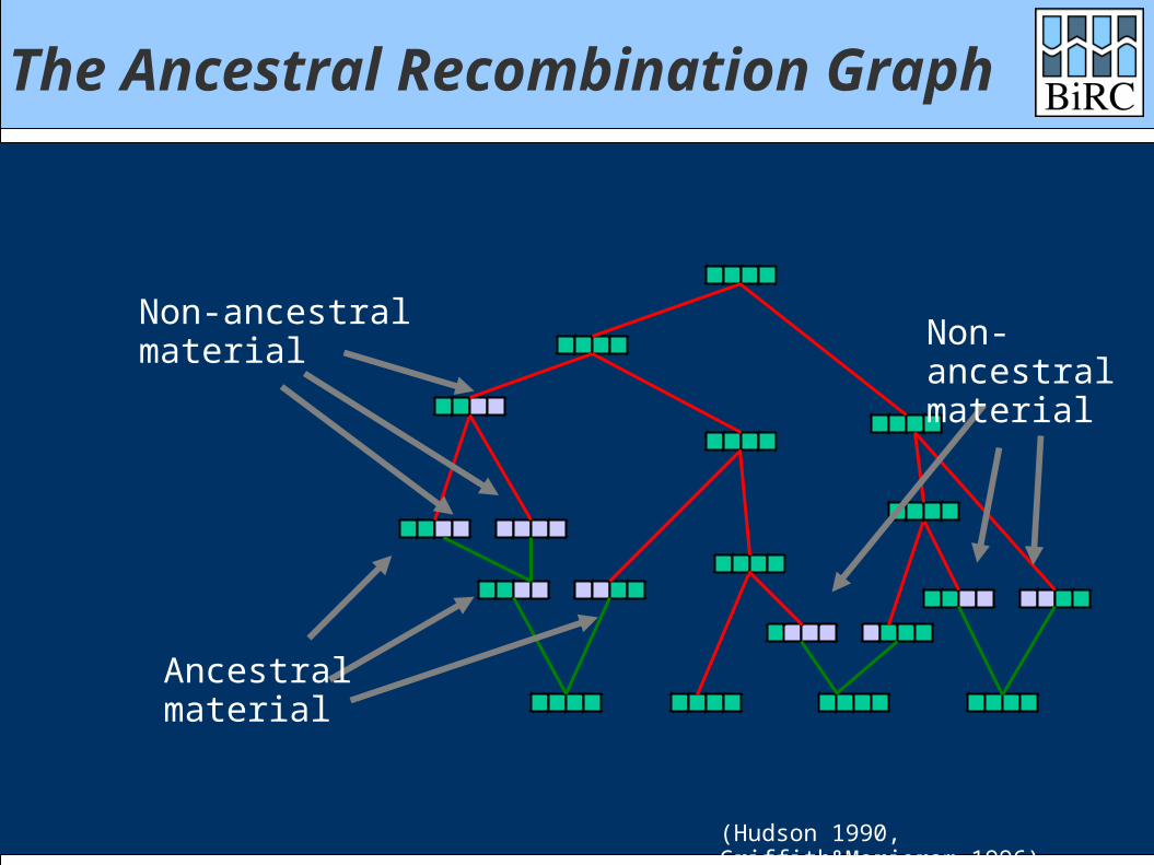
The Ancestral Recombination Graph
Non-ancestralmaterial Non-
ancestralmaterial
Ancestralmaterial
(Hudson 1990, Griffith&Marjoram 1996)
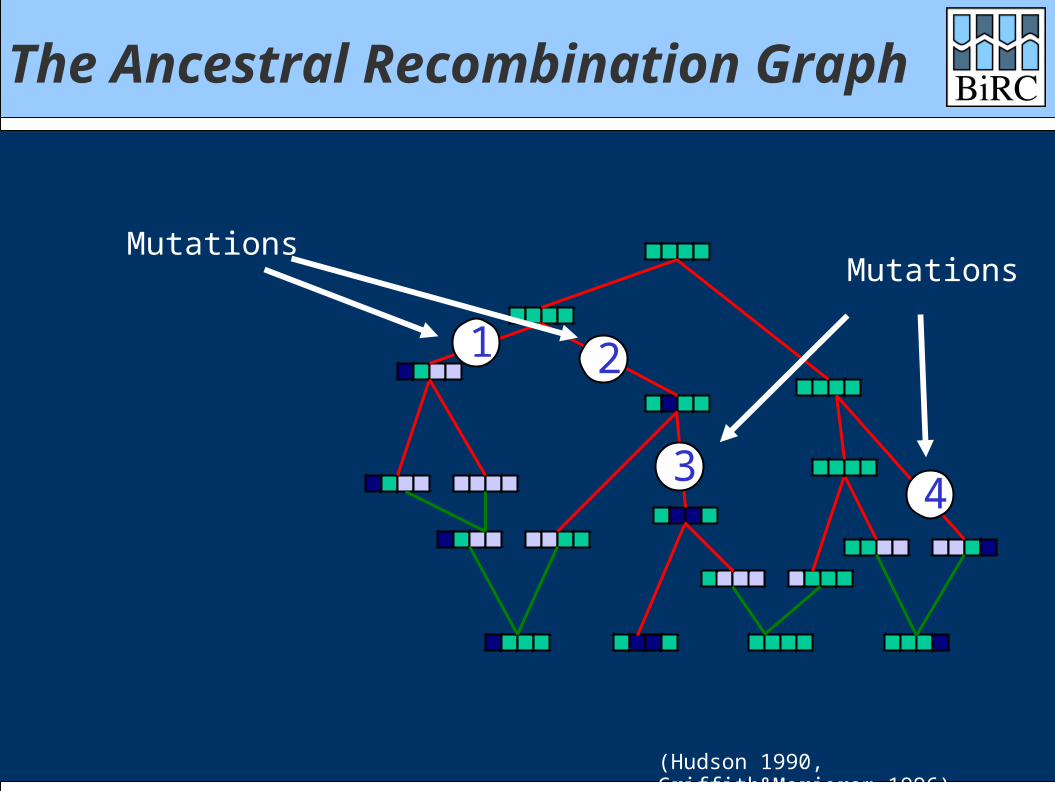
The Ancestral Recombination Graph
MutationsMutations
1 2
34
(Hudson 1990, Griffith&Marjoram 1996)
(Larribe, Lessard and Schork, 2002)
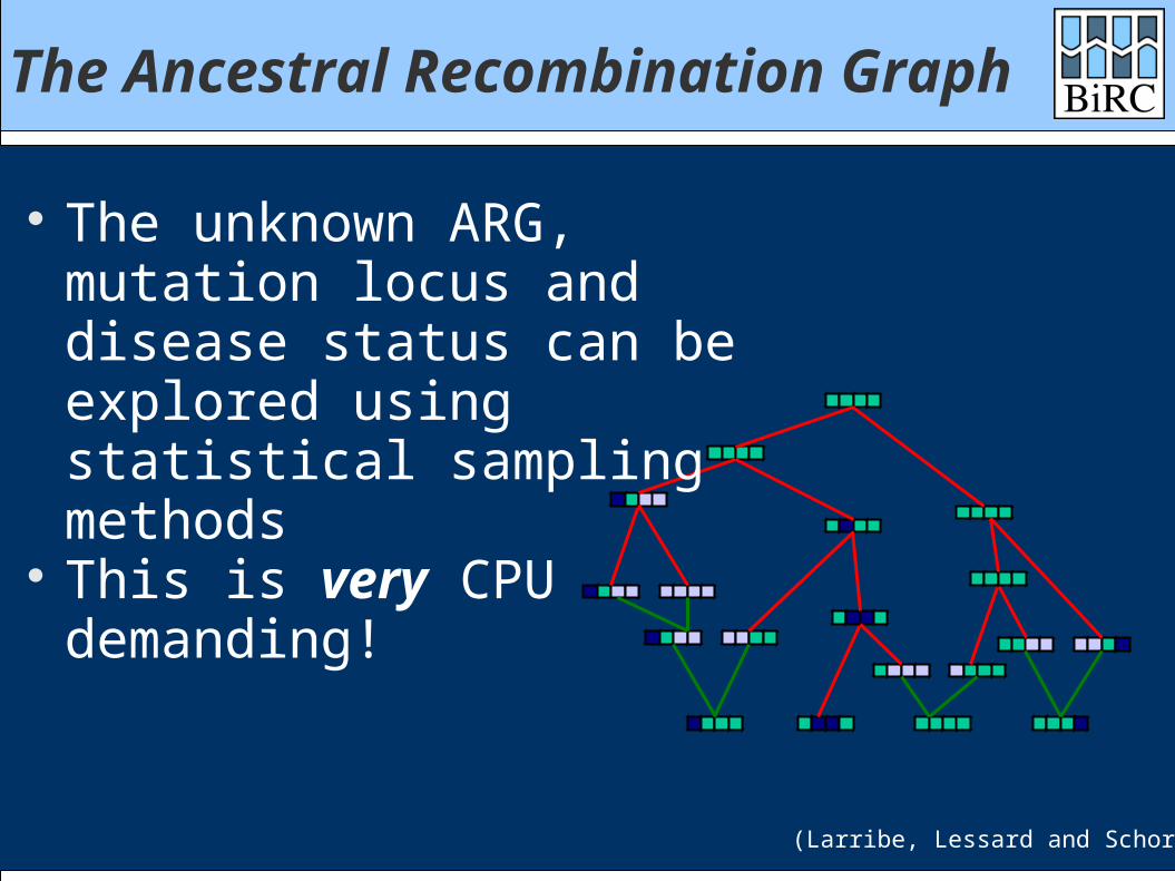
The unknown ARG, mutation locus and disease status can be explored using statistical sampling methods
This is very CPU demanding!
The Ancestral Recombination Graph
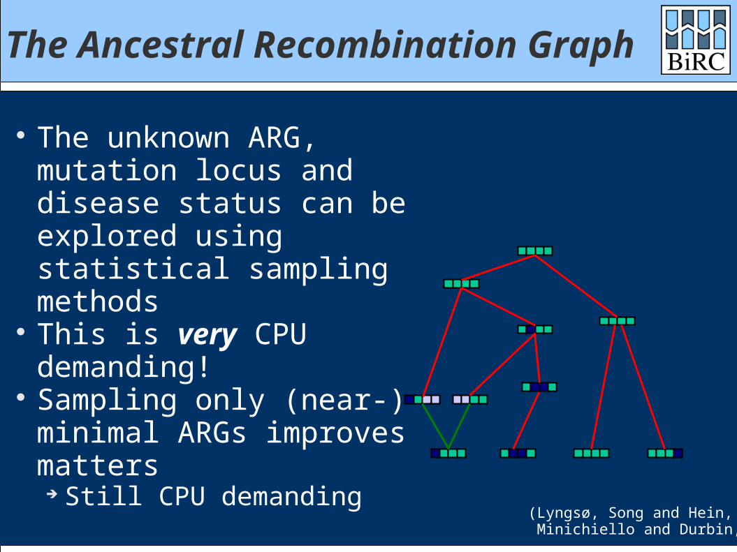
(Lyngsø, Song and Hein, 2005; Minichiello and Durbin, 2006)
The unknown ARG, mutation locus and disease status can be explored using statistical sampling methods
This is very CPU demanding!
Sampling only (near-) minimal ARGs improves matters
Still CPU demanding
The Ancestral Recombination Graph
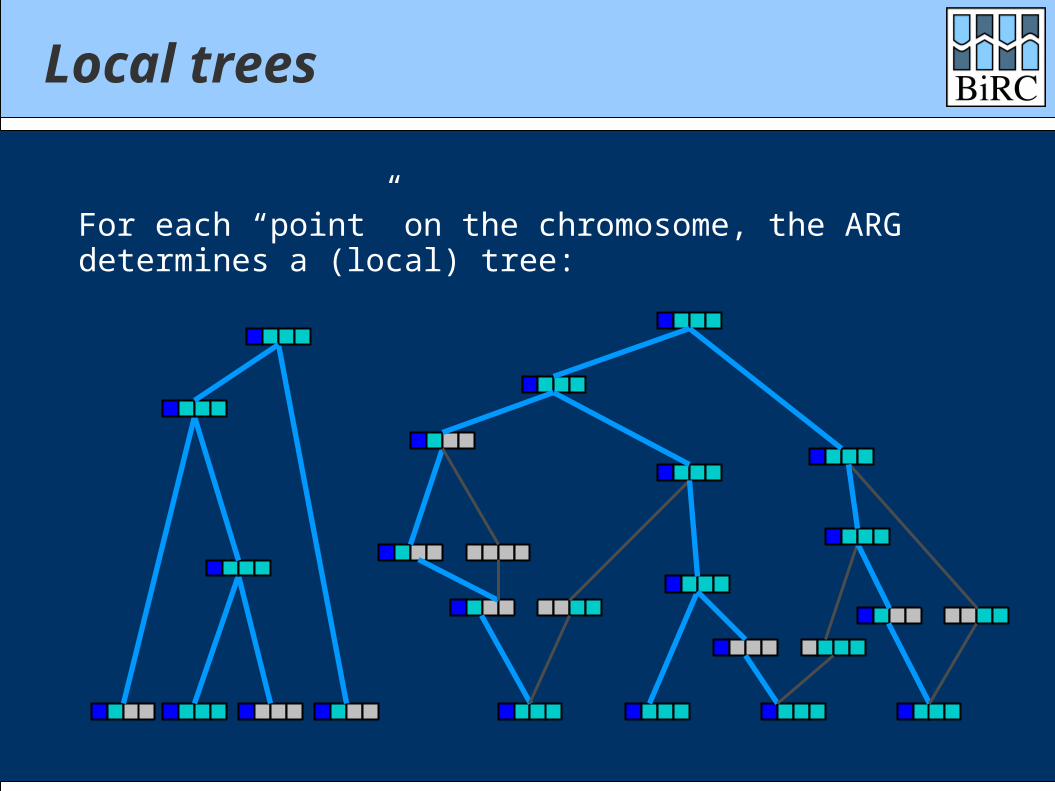
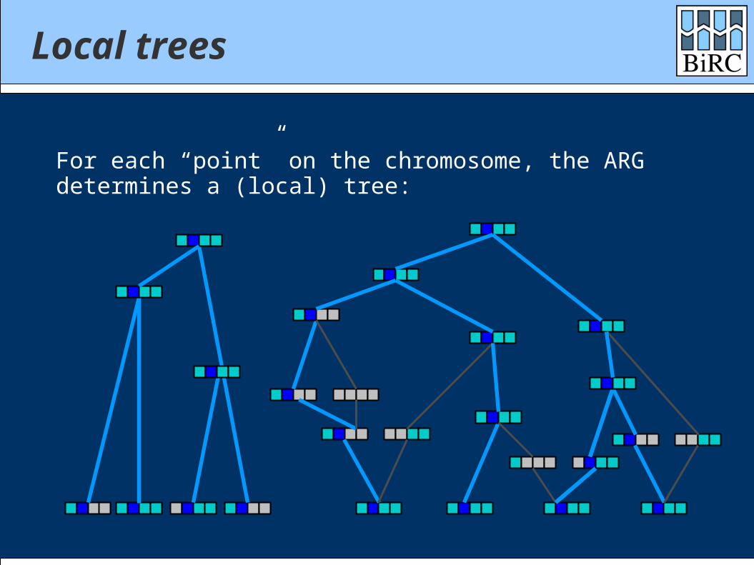
Local trees
For each “point” on the chromosome, the ARGdetermines a (local) tree:
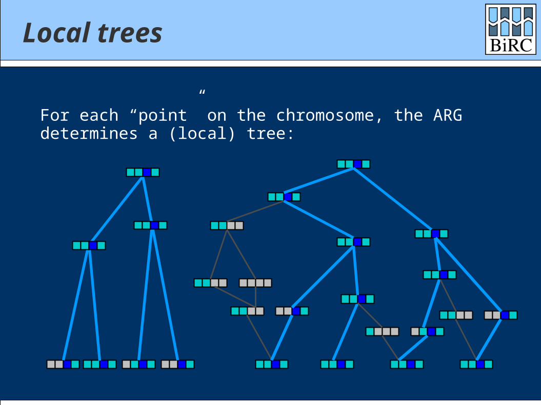
Local trees
For each “point” on the chromosome, the ARGdetermines a (local) tree:
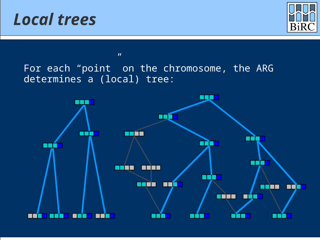
Local trees
For each “point” on the chromosome, the ARGdetermines a (local) tree:
Local trees
For each “point” on the chromosome, the ARGdetermines a (local) tree:
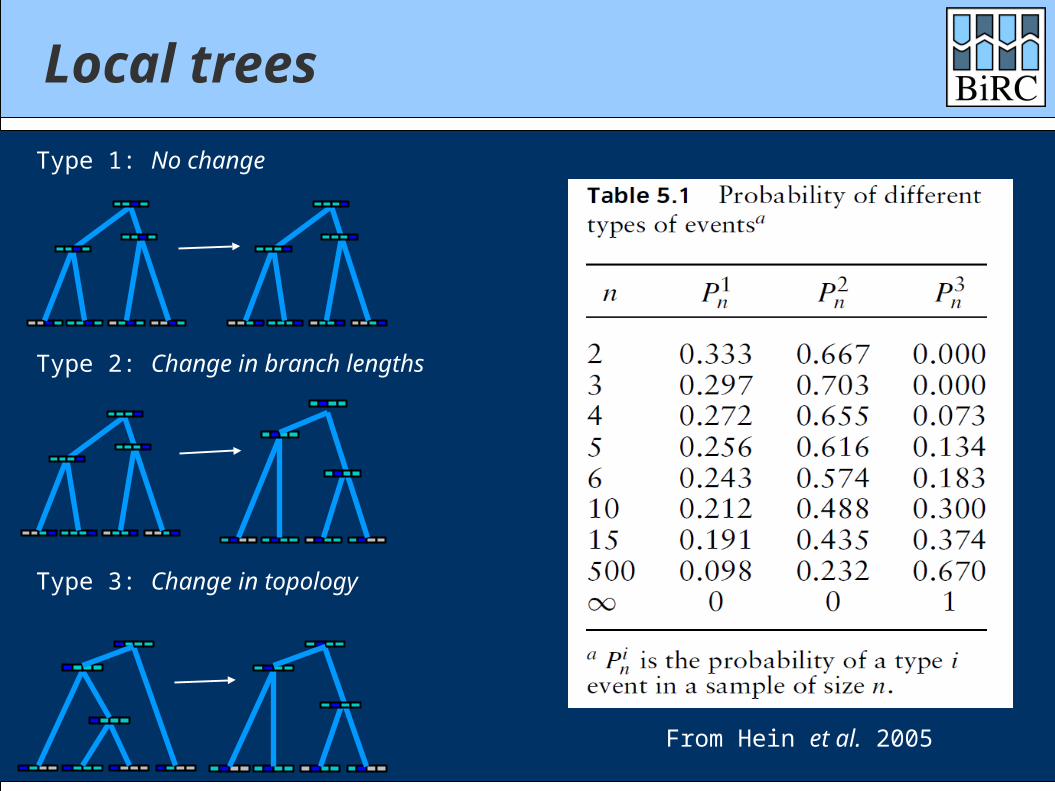
Local trees
Type 1: No change
Type 2: Change in branch lengths
Type 3: Change in topology
From Hein et al. 2005
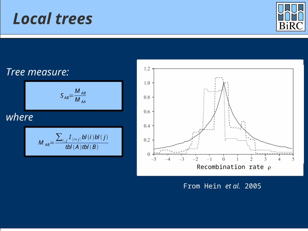
Local trees
Recombination rate
From Hein et al. 2005
Tree measure:
M AB=∑i , j
I {i= j }bl i bl j
tbl A tbl B
S AB=M AB
M AA
where
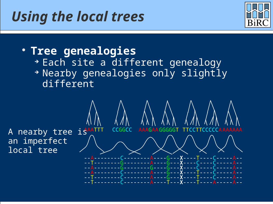
Using the local trees
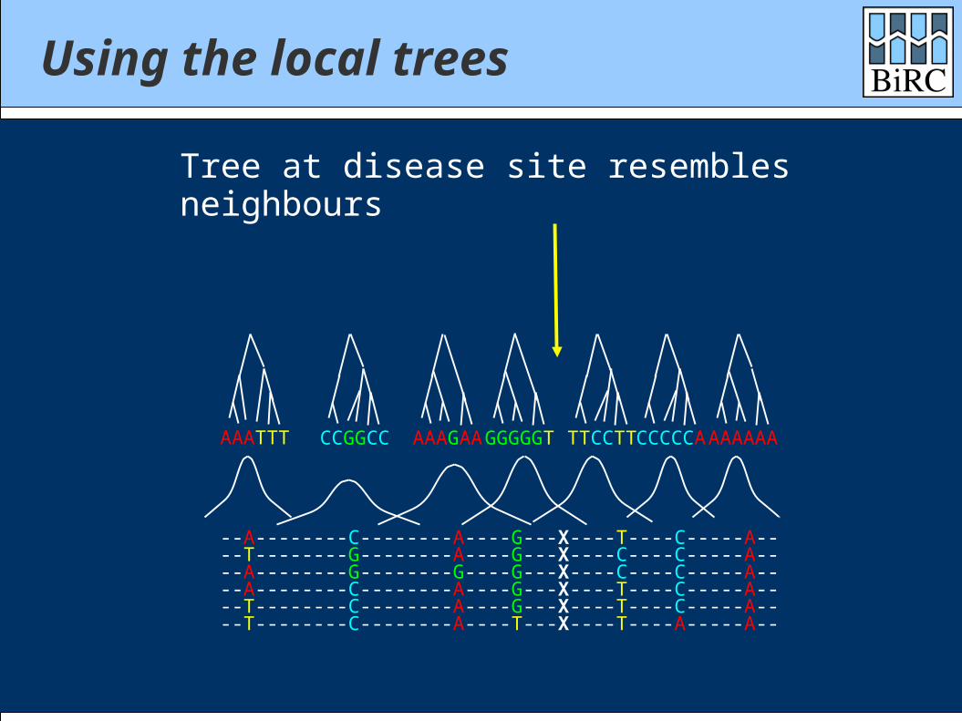
Tree genealogies Each site a different genealogy Nearby genealogies only slightly different
--T--------G--------A----G---X----C----C-----A----A--------G--------G----G---X----C----C-----A----A--------C--------A----G---X----T----C-----A----T--------C--------A----G---X----T----C-----A----T--------C--------A----T---X----T----A-----A--
--A--------C--------A----G---X----T----C-----A--
AAATTT CCGGCC AAAGAAGGGGGT TTCCTTCCCCCAAAAAAAA nearby tree isan imperfectlocal tree
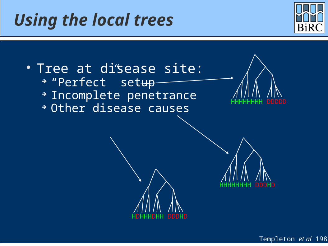
Tree at disease site: “Perfect” setup Incomplete penetrance Other disease causes
HHHHHHHH DDDDD
HHHHHHHH DDDHD
HDHHHDHH DDDHD
Templeton et al 1987
Using the local trees
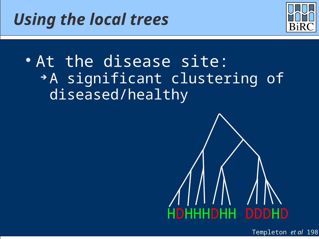
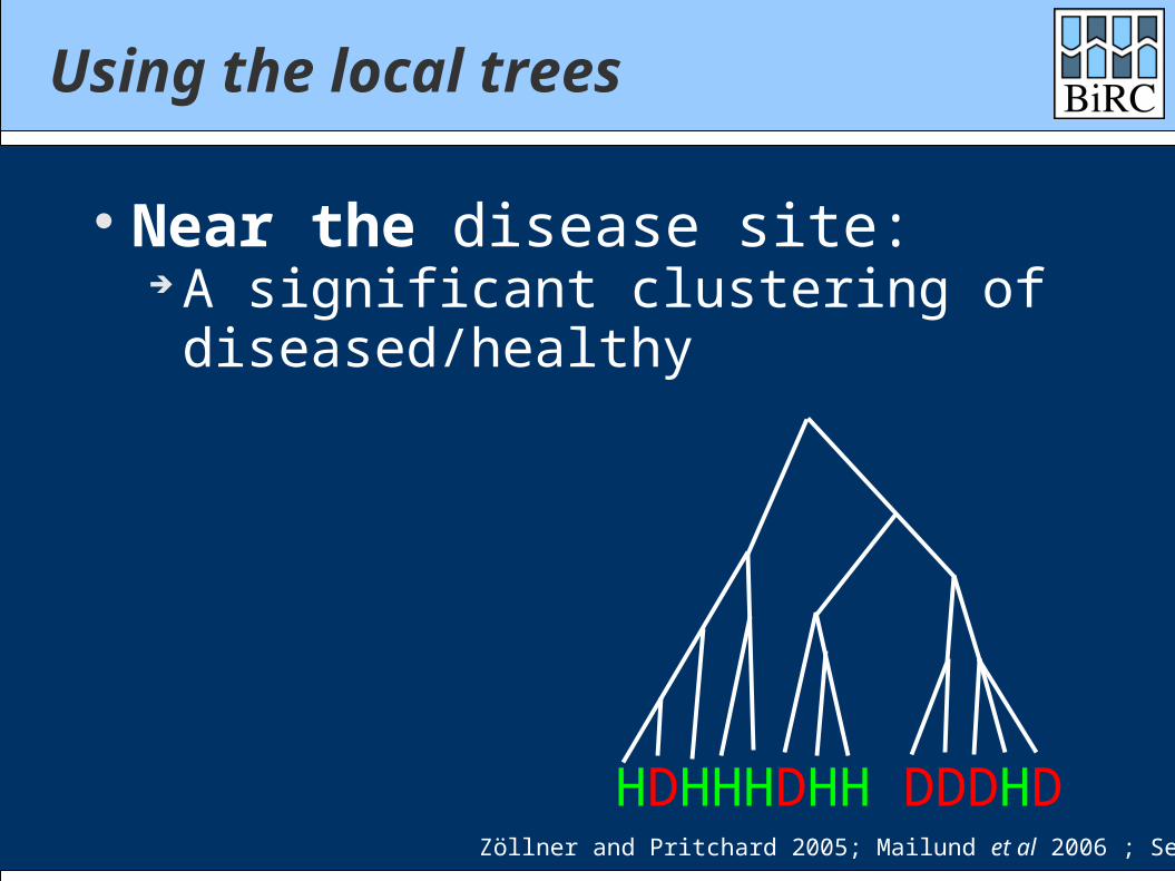
At the disease site: A significant clustering of
diseased/healthy
HDHHHDHH DDDHD
Using the local trees
Templeton et al 1987
--T--------G--------A----G---X----C----C-----A----A--------G--------G----G---X----C----C-----A----A--------C--------A----G---X----T----C-----A----T--------C--------A----G---X----T----C-----A----T--------C--------A----T---X----T----A-----A--
--A--------C--------A----G---X----T----C-----A--
AAATTT CCGGCC AAAGAAGGGGGT TTCCTTCCCCCAAAAAAA
Tree at disease site resembles neighbours
Using the local trees
Near the disease site: A significant clustering of
diseased/healthy
HDHHHDHH DDDHD
Using the local trees
Zöllner and Pritchard 2005; Mailund et al 2006 ; Sevon et al 2006
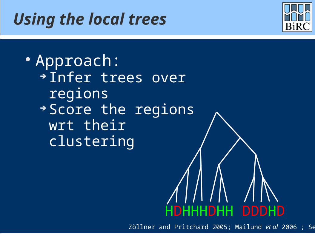
Approach: Infer trees over regions Score the regions wrt
their clustering
HDHHHDHH DDDHDZöllner and Pritchard 2005; Mailund et al 2006 ; Sevon et al 2006
Using the local trees
In the infinite sites model: Each mutation occurs only once Each mutation splits the sample in two A consistent tree can efficiently be inferred
for a recombination free region
Mailund et al 2006
BLOck aSSOCiation (BLOSSOC)
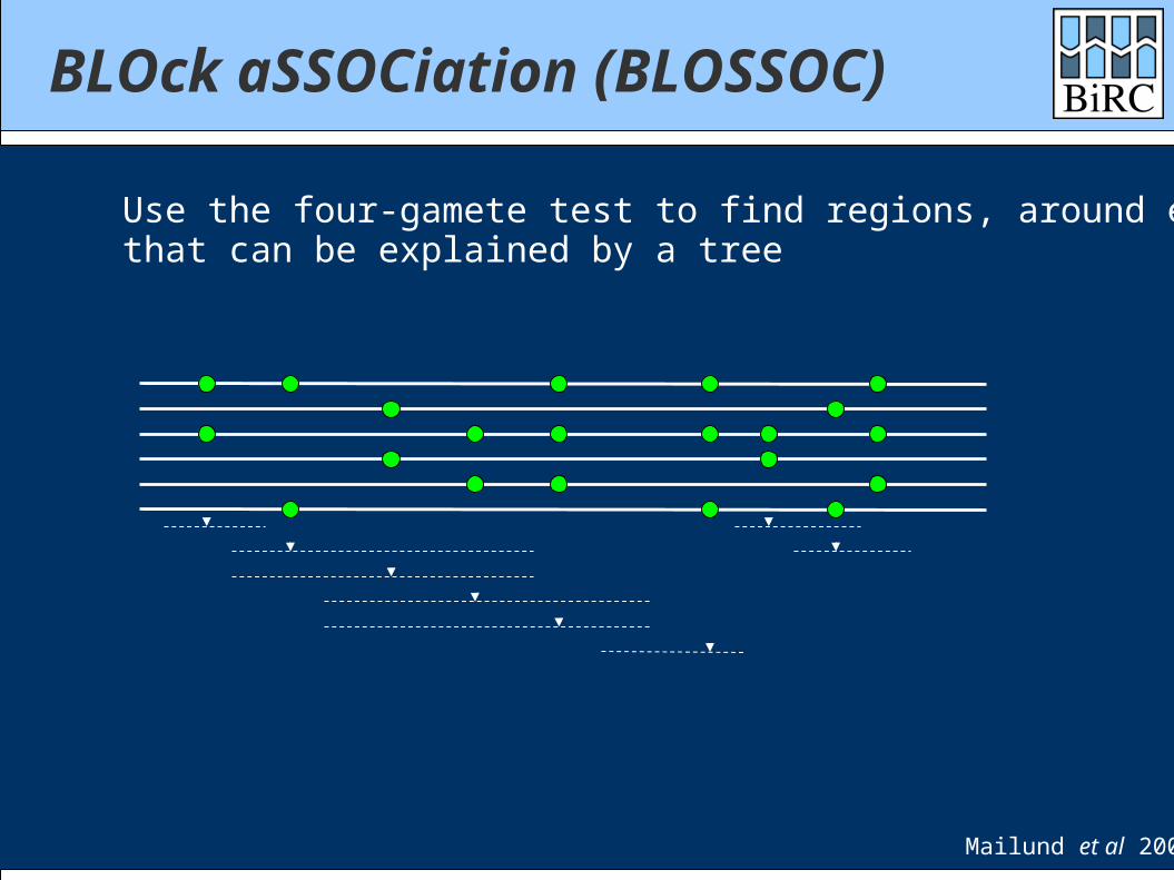
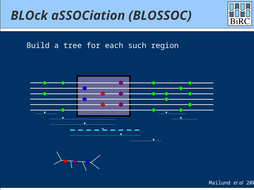
Use the four-gamete test to find regions, around each locus,that can be explained by a tree
Mailund et al 2006
BLOck aSSOCiation (BLOSSOC)
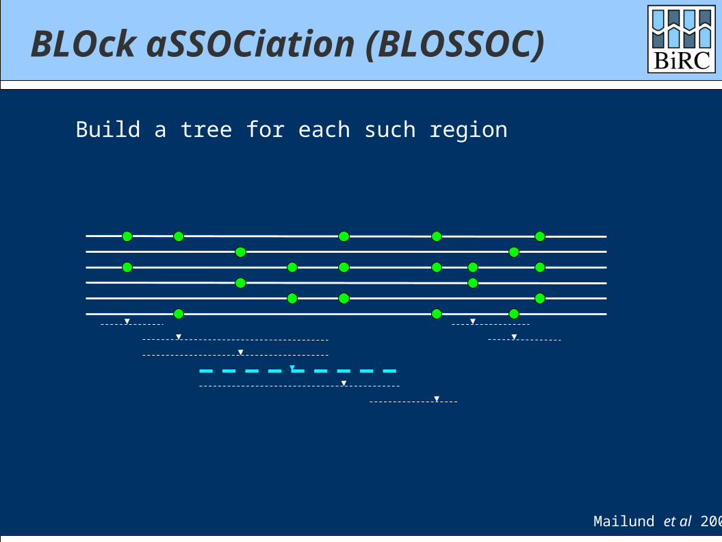
Build a tree for each such region
Mailund et al 2006
BLOck aSSOCiation (BLOSSOC)
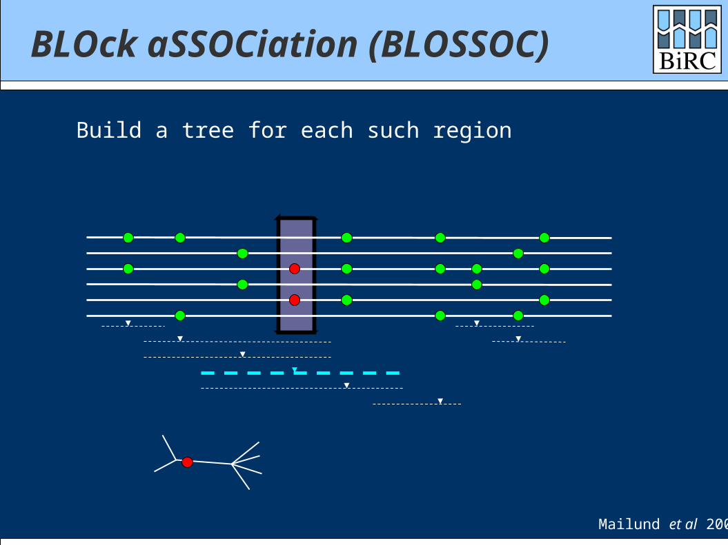
Build a tree for each such region
Mailund et al 2006
BLOck aSSOCiation (BLOSSOC)
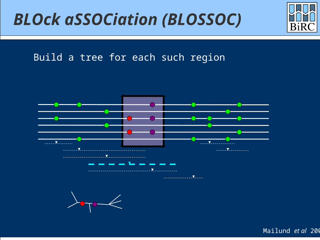
Build a tree for each such region
Mailund et al 2006
BLOck aSSOCiation (BLOSSOC)
Build a tree for each such region
Mailund et al 2006
BLOck aSSOCiation (BLOSSOC)
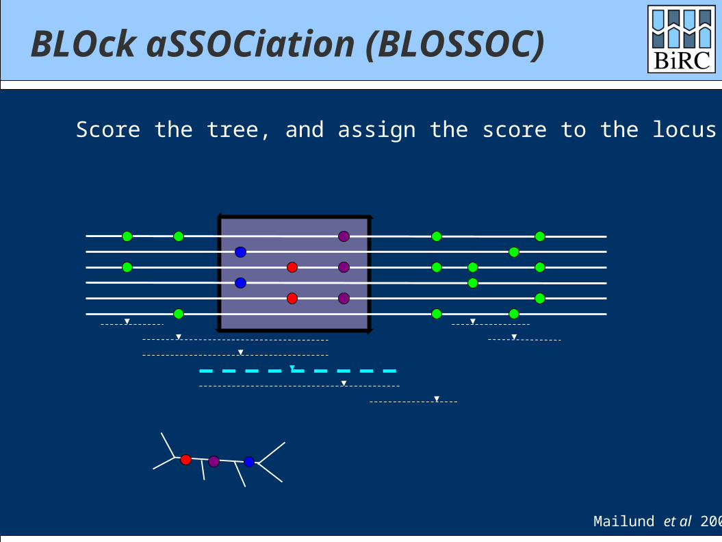
Score the tree, and assign the score to the locus
Mailund et al 2006
BLOck aSSOCiation (BLOSSOC)
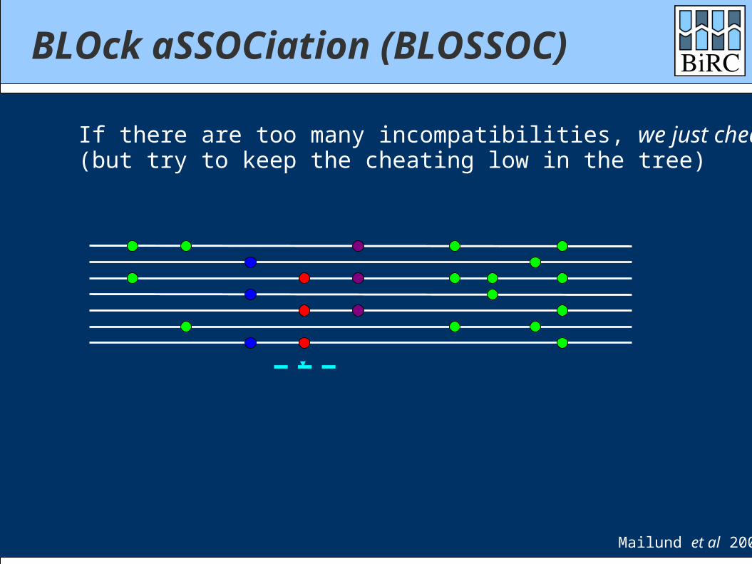
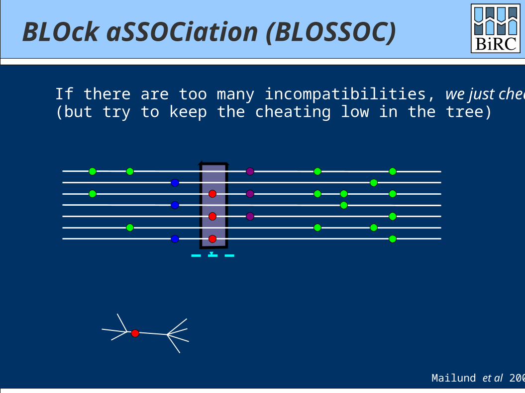
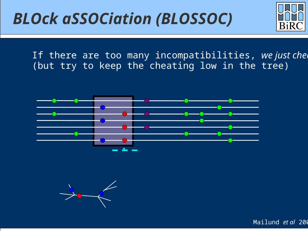
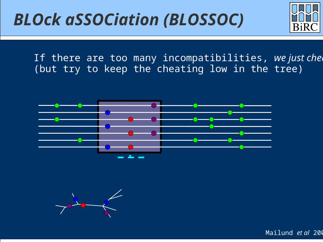
If there are too many incompatibilities, we just cheat(but try to keep the cheating low in the tree)
Mailund et al 2006
BLOck aSSOCiation (BLOSSOC)
If there are too many incompatibilities, we just cheat(but try to keep the cheating low in the tree)
Mailund et al 2006
BLOck aSSOCiation (BLOSSOC)
If there are too many incompatibilities, we just cheat(but try to keep the cheating low in the tree)
Mailund et al 2006
BLOck aSSOCiation (BLOSSOC)
If there are too many incompatibilities, we just cheat(but try to keep the cheating low in the tree)
Mailund et al 2006
BLOck aSSOCiation (BLOSSOC)
BLOck aSSOCiation (BLOSSOC)
Ding et al 2007
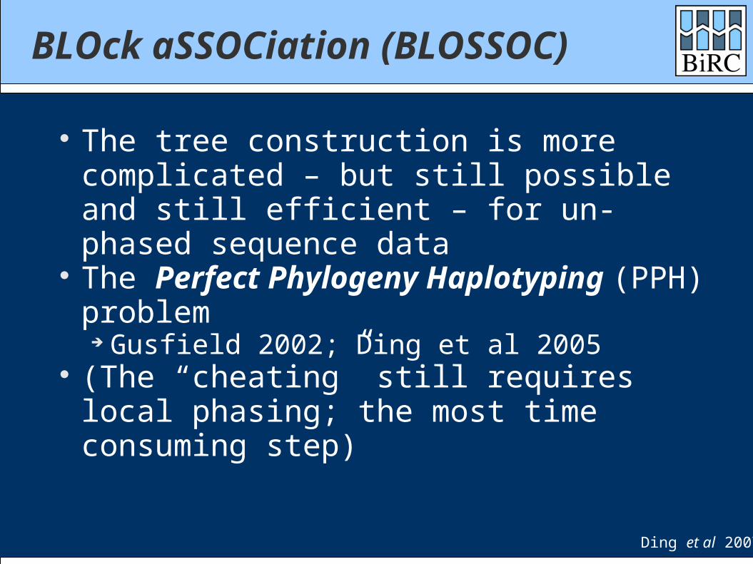
The tree construction is more complicated – but still possible and still efficient – for un-phased sequence data
The Perfect Phylogeny Haplotyping (PPH) problem
Gusfield 2002; Ding et al 2005 (The “cheating” still requires local
phasing; the most time consuming step)
BLOck aSSOCiation (BLOSSOC)
Ding et al 2007
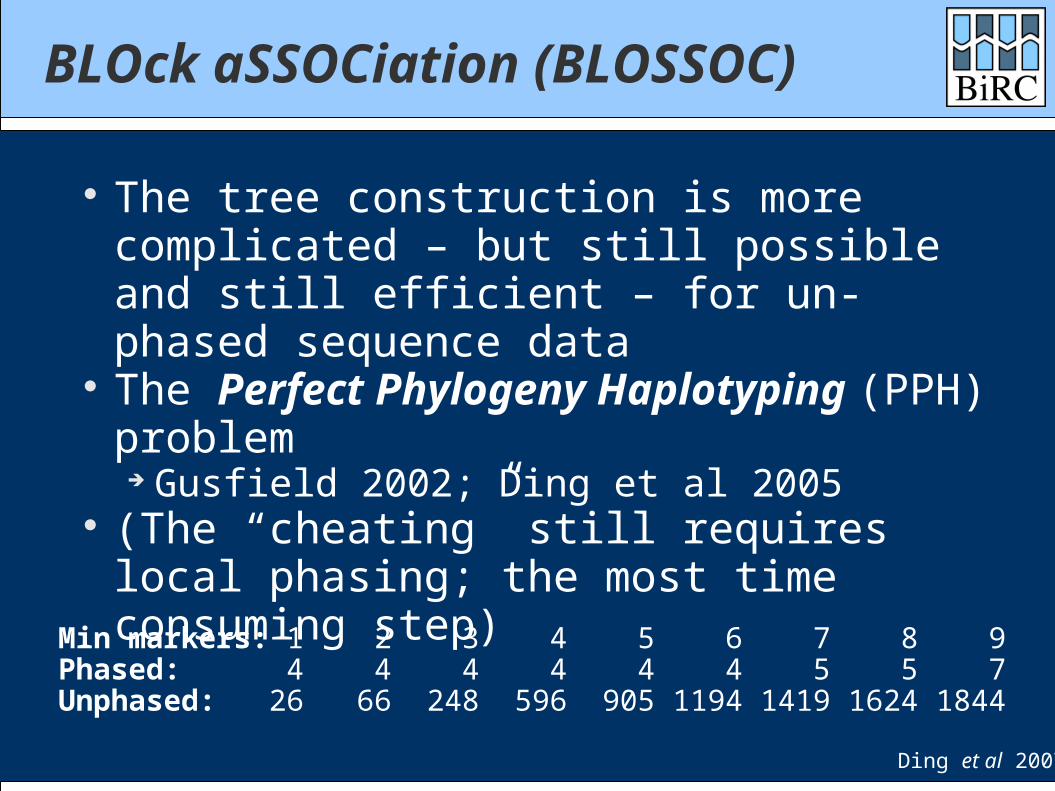
The tree construction is more complicated – but still possible and still efficient – for un-phased sequence data
The Perfect Phylogeny Haplotyping (PPH) problem
Gusfield 2002; Ding et al 2005 (The “cheating” still requires local
phasing; the most time consuming step)Min markers: 1 2 3 4 5 6 7 8 9Phased: 4 4 4 4 4 4 5 5 7Unphased: 26 66 248 596 905 1194 1419 1624 1844
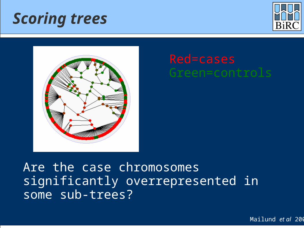
Scoring trees
Red=casesGreen=controls
Are the case chromosomes significantly overrepresented in some sub-trees?
Mailund et al 2006
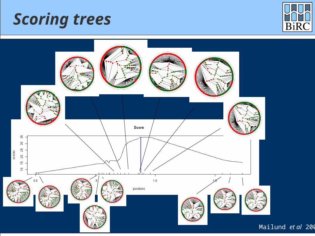
Scoring trees
Mailund et al 2006
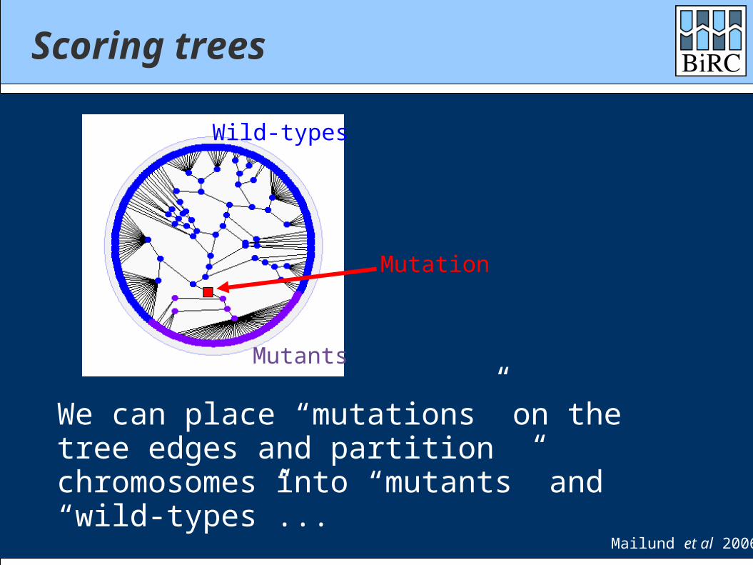
Scoring trees
Mutation
We can place “mutations” on the tree edges and partition chromosomes into “mutants” and “wild-types”...
Mailund et al 2006
Mutants
Wild-types
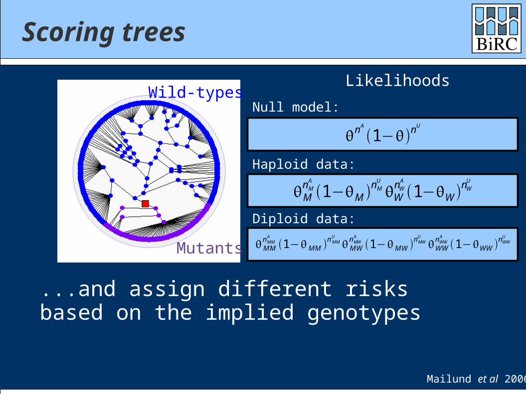
Scoring trees
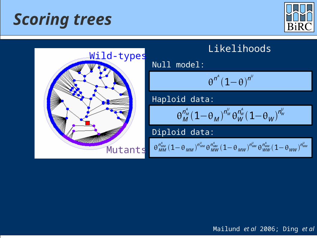
...and assign different risks based on the implied genotypes
Mutants
Wild-types
nA
1−nU
MMnMMA
1−MM n MMU
MWnMWA
1−MW nMWU
WWnWWA
1−WW nWWU
Likelihoods
Haploid data:
MnMA
1−M nMU
WnWA
1−W nWU
Null model:
Diploid data:
Mailund et al 2006
Scoring trees
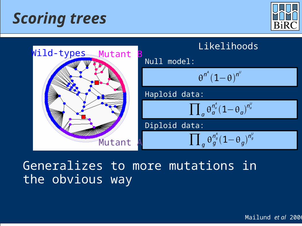
Generalizes to more mutations in the obvious way
nA
1−nU
Likelihoods
Haploid data:
∏aanaA
1−anaU
Null model:
Diploid data:
Mailund et al 2006
∏ ggn gA
1−gn gU
Wild-types
Mutant A
Mutant B
Scoring trees
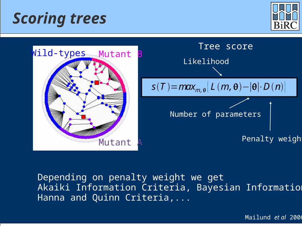
s T =maxm , {L m ,−∣∣⋅Dn}
Tree score
Mailund et al 2006
Wild-types
Mutant A
Mutant BLikelihood
Number of parameters
Penalty weight
Depending on penalty weight we getAkaiki Information Criteria, Bayesian Information Criteria,Hanna and Quinn Criteria,...
Scoring trees
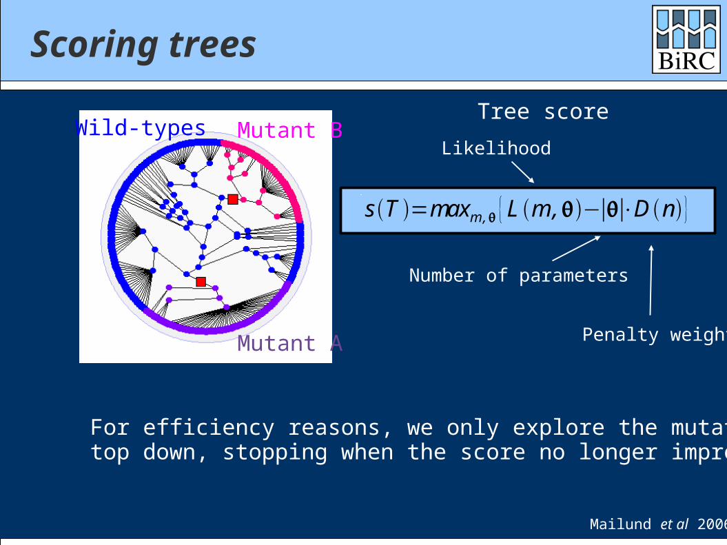
s T =maxm , {L m ,−∣∣⋅Dn}
Tree score
Mailund et al 2006
Wild-types
Mutant A
Mutant BLikelihood
Number of parameters
Penalty weight
For efficiency reasons, we only explore the mutationstop down, stopping when the score no longer improves
Scoring trees
Mailund et al 2006; Ding et al 2007
Mutants
Wild-types
nA
1−nU
MMnMMA
1−MM n MMU
MWnMWA
1−MW nMWU
WWnWWA
1−WW nWWU
Likelihoods
Haploid data:
MnMA
1−M nMU
WnWA
1−W nWU
Null model:
Diploid data:
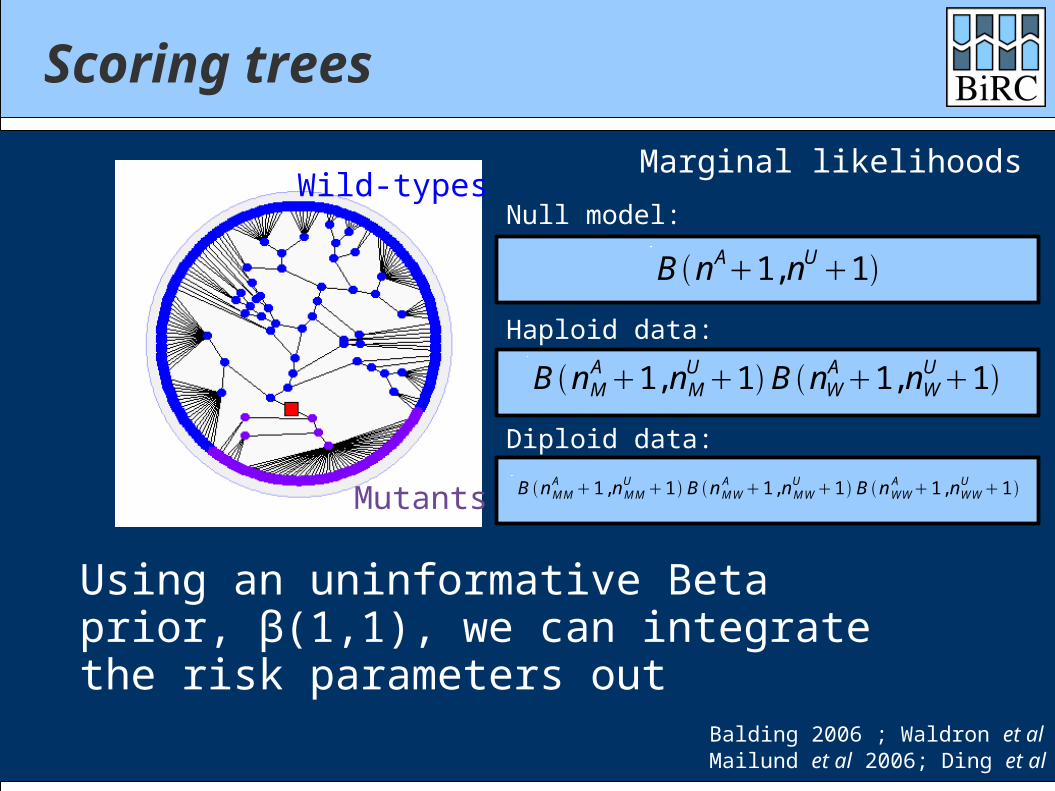
Scoring trees
Using an uninformative Beta prior, β(1,1), we can integrate the risk parameters out
Mailund et al 2006; Ding et al 2007
Mutants
Wild-types
B nA1, nU1
B nMMA 1, nMM
U 1 B nMWA 1, nMW
U 1 B nWWA 1, nWW
U 1
Marginal likelihoods
Haploid data:
B nMA 1, nM
U 1B nWA 1, nW
U 1
Null model:
Diploid data:
Balding 2006 ; Waldron et al 2006
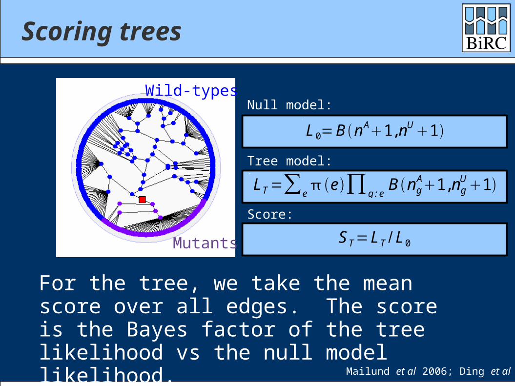
Scoring trees
For the tree, we take the mean score over all edges. The score is the Bayes factor of the tree likelihood vs the null model likelihood.
Mailund et al 2006; Ding et al 2007
Mutants
Wild-types
L0=B n A1, nU1
LT=∑e e ∏g :e
B ngA1, ng
U1
Null model:
Tree model:
Score:
S T=LT / L0
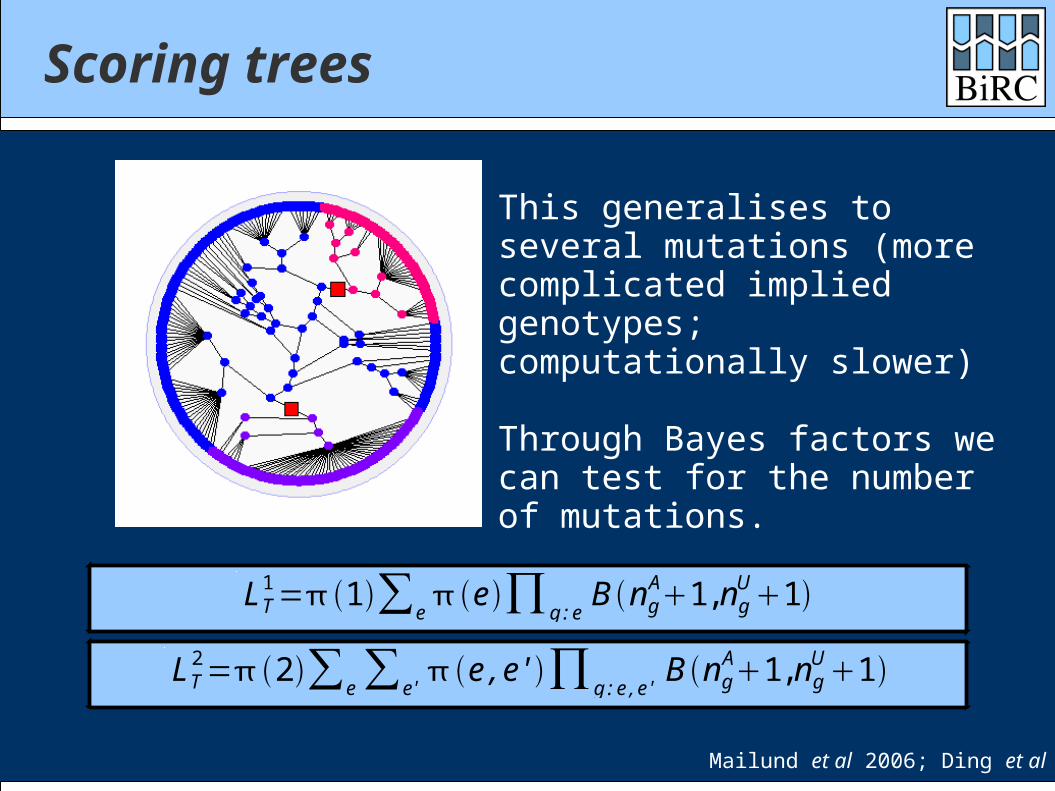
Scoring trees
This generalises to several mutations (more complicated implied genotypes; computationally slower)
Through Bayes factors we can test for the number of mutations.
Mailund et al 2006; Ding et al 2007
LT1=1∑e
e ∏g :eB ng
A1, ngU1
LT2=2 ∑e∑e '
e , e ' ∏g :e , e 'B ng
A1, ngU1
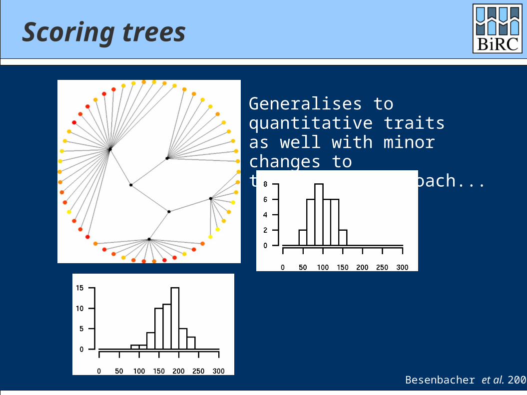
Scoring trees
Generalises to quantitative traitsas well with minor changes tothe scoring approach...
Besenbacher et al. 2007
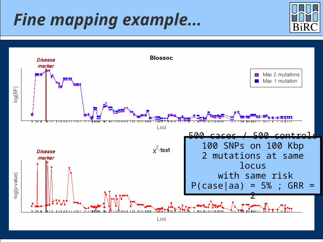
Fine mapping example...
500 cases / 500 controls100 SNPs on 100 Kbp
2 mutations at same locus with same risk
P(case|aa) = 5% ; GRR = 2
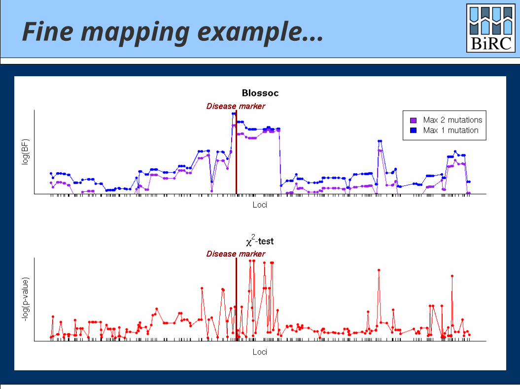
Fine mapping example...
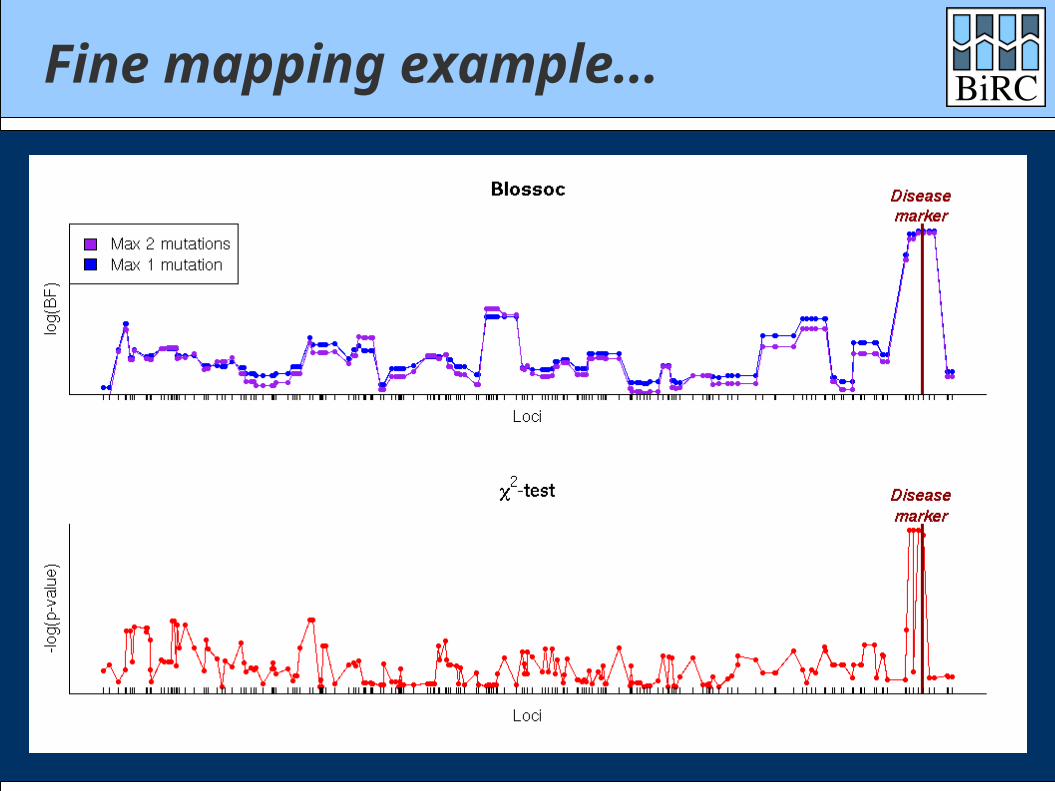
Fine mapping example...

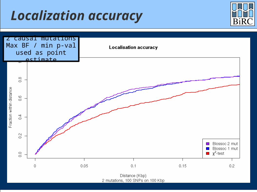
Localization accuracy
1 causal mutationMax BF / min p-val
used as point estimate
Localization accuracy
2 causal mutationsMax BF / min p-val
used as point estimate
Comparison with Margarita
Margarita is the (near-)minimal ARG method of Minichiello and Durbin
Data sets: 1000 cases / 1000 controls 300 markers
Comparisons with both phased and unphased data
Acknowledgment: Experiments done by Yun S. Song

Comparison with MargaritaUnphased data; Min markers: 5

Comparison with MargaritaPhased data; Min markers: 5
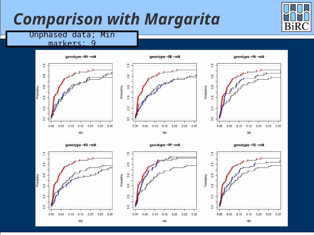
Comparison with MargaritaUnphased data; Min markers: 9
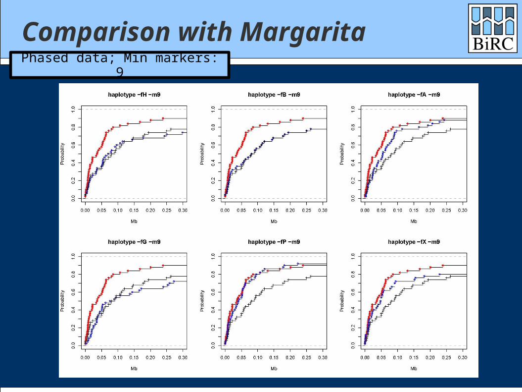
Comparison with MargaritaPhased data; Min markers: 9
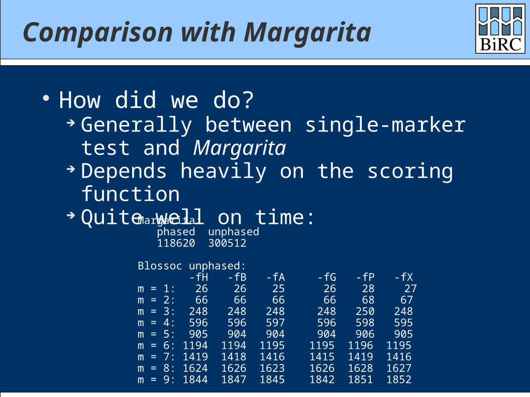
Comparison with Margarita
How did we do? Generally between single-marker test and
Margarita Depends heavily on the scoring function Quite well on time:
Margarita: phased unphased 118620 300512
Blossoc unphased: -fH -fB -fA -fG -fP -fXm = 1: 26 26 25 26 28 27 m = 2: 66 66 66 66 68 67 m = 3: 248 248 248 248 250 248 m = 4: 596 596 597 596 598 595 m = 5: 905 904 904 904 906 905 m = 6: 1194 1194 1195 1195 1196 1195m = 7: 1419 1418 1416 1415 1419 1416m = 8: 1624 1626 1623 1626 1628 1627m = 9: 1844 1847 1845 1842 1851 1852
Choice of scoring function
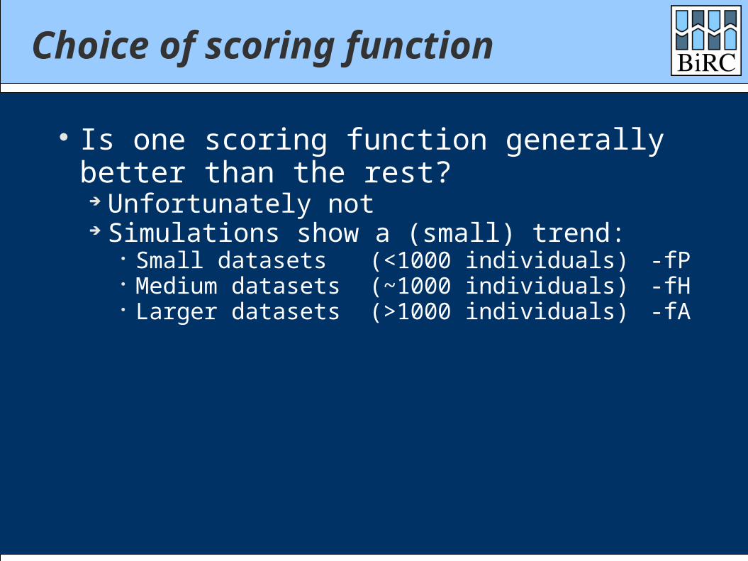
Is one scoring function generally better than the rest?
Unfortunately not Simulations show a (small) trend:
Small datasets (<1000 individuals) -fP Medium datasets (~1000 individuals) -fH Larger datasets (>1000 individuals) -fA
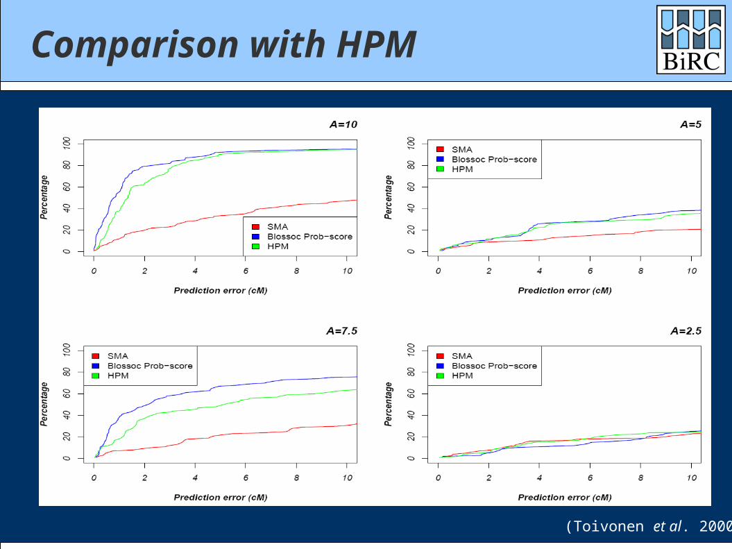
Comparison with HPM
(Toivonen et al. 2000)
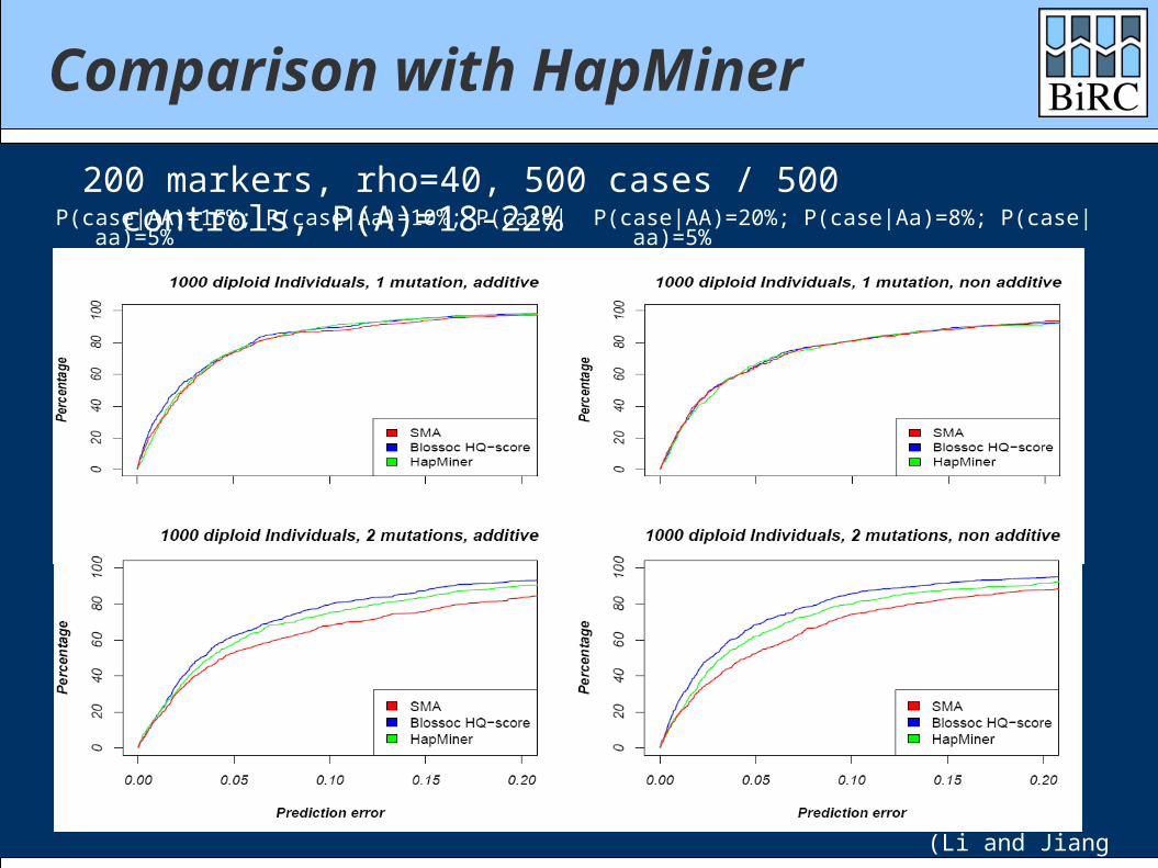
Comparison with HapMiner
P(case|AA)=15%; P(case|Aa)=10%; P(case|aa)=5%
200 markers, rho=40, 500 cases / 500 controls, P(A)=18-22% P(case|AA)=20%; P(case|Aa)=8%; P(case|aa)=5%
(Li and Jiang 2005)
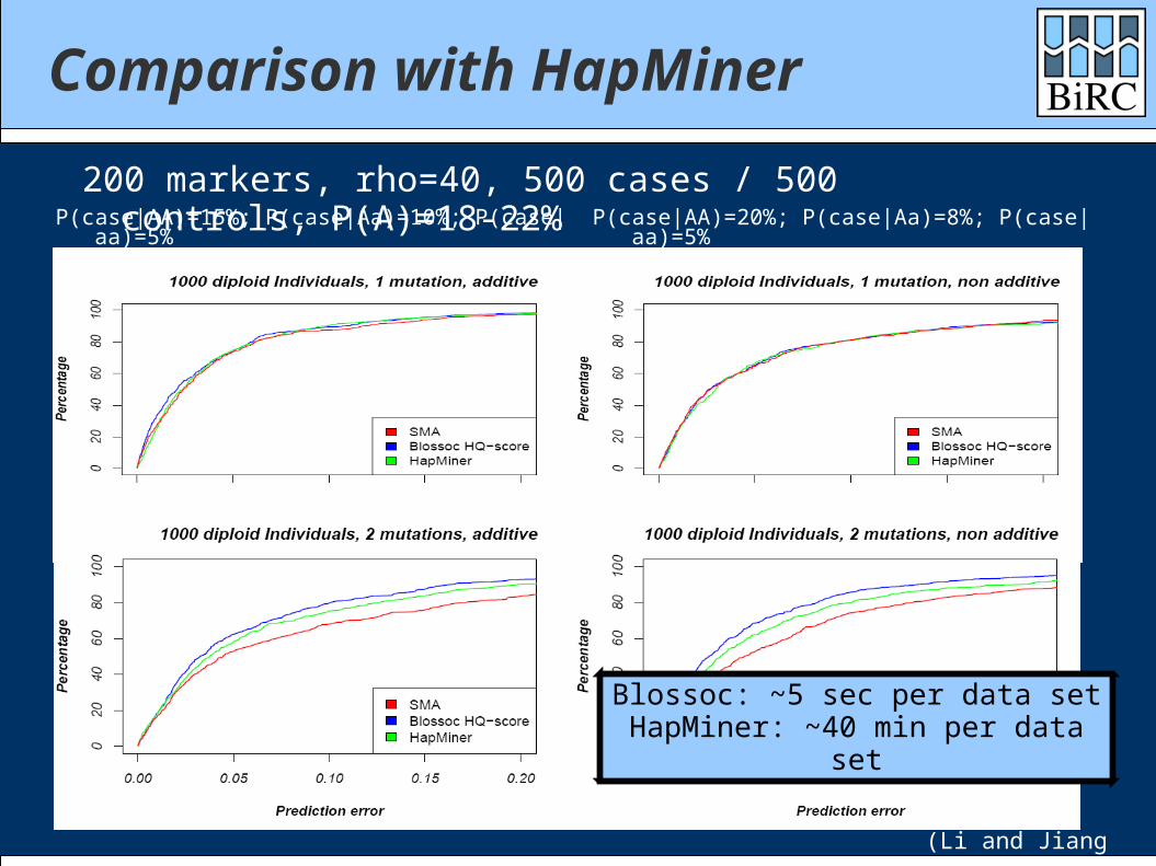
Comparison with HapMiner
P(case|AA)=15%; P(case|Aa)=10%; P(case|aa)=5%
200 markers, rho=40, 500 cases / 500 controls, P(A)=18-22% P(case|AA)=20%; P(case|Aa)=8%; P(case|aa)=5%
(Li and Jiang 2005)
Blossoc: ~5 sec per data setHapMiner: ~40 min per data set
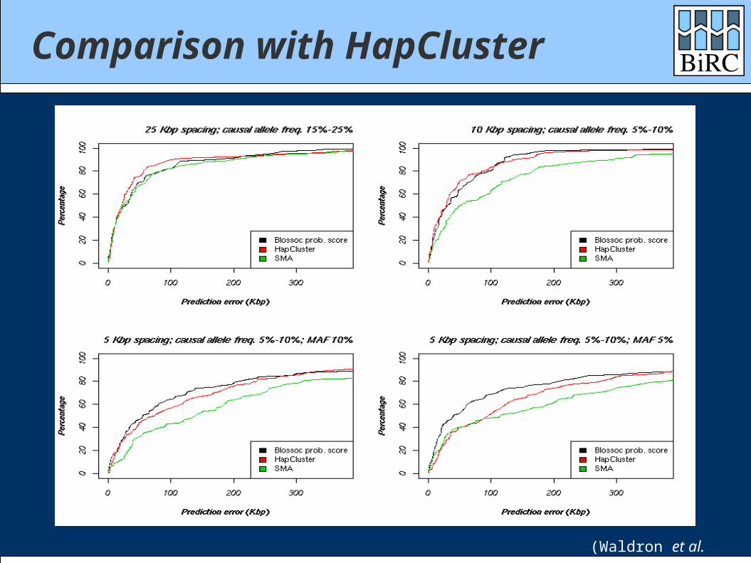
Comparison with HapCluster
(Waldron et al. 2006)
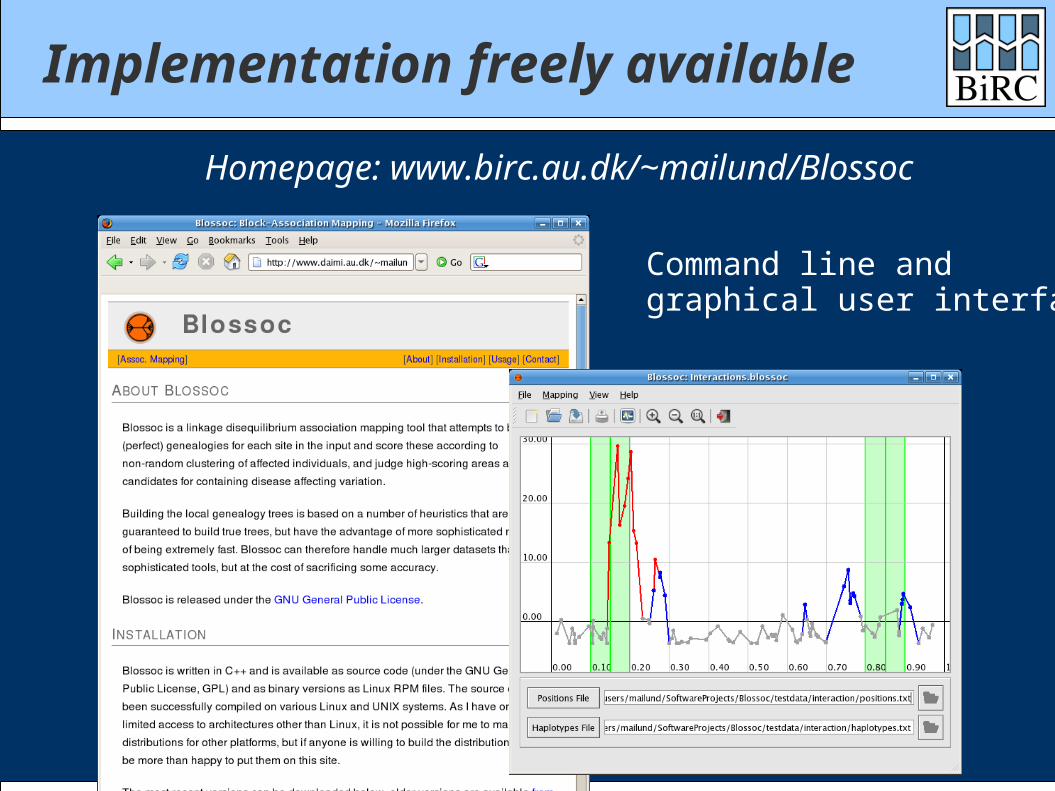
Implementation freely available
Homepage: www.birc.au.dk/~mailund/Blossoc
Command line andgraphical user interface...
The end
Thank you!
More at http://www.birc.au.dk/~mailund/association-mapping/
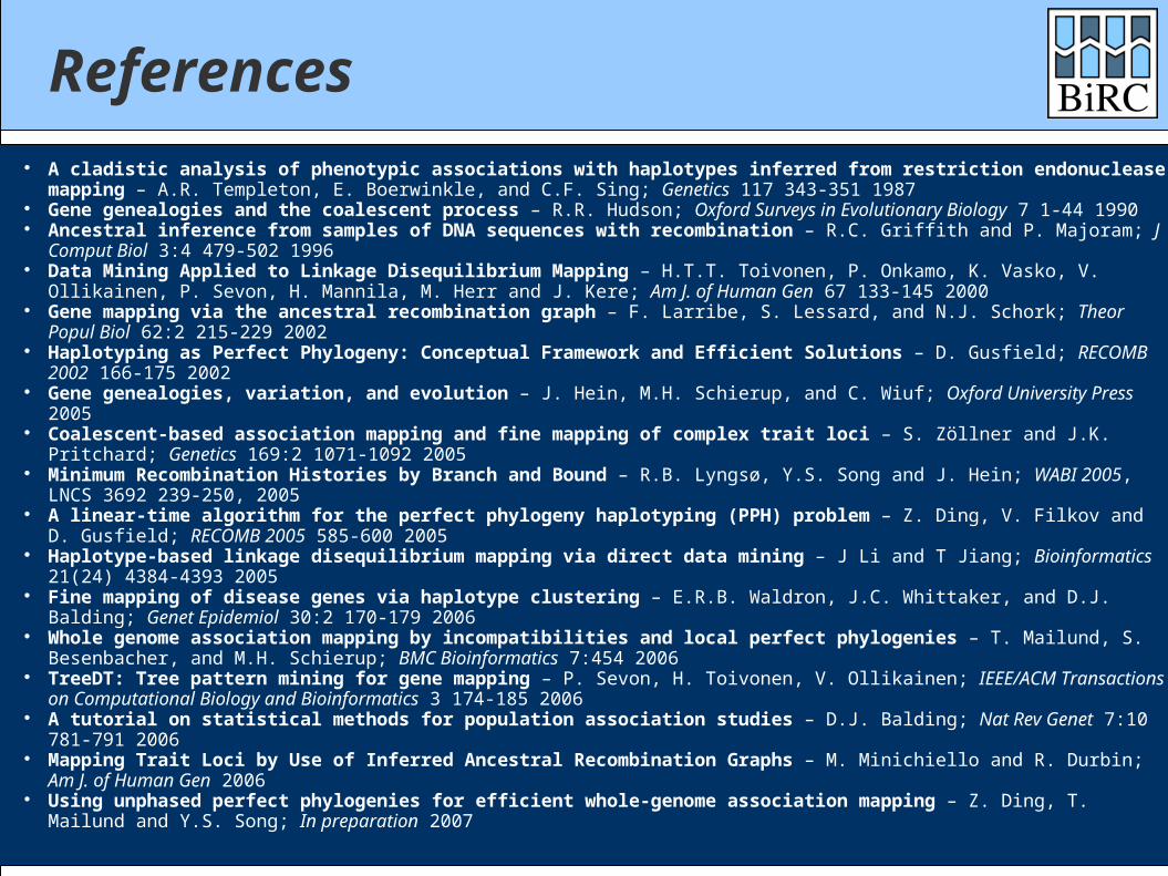
References A cladistic analysis of phenotypic associations with haplotypes inferred from restriction endonuclease mapping – A.R.
Templeton, E. Boerwinkle, and C.F. Sing; Genetics 117 343-351 1987 Gene genealogies and the coalescent process – R.R. Hudson; Oxford Surveys in Evolutionary Biology 7 1-44 1990 Ancestral inference from samples of DNA sequences with recombination – R.C. Griffith and P. Majoram; J Comput Biol 3:4
479-502 1996 Data Mining Applied to Linkage Disequilibrium Mapping – H.T.T. Toivonen, P. Onkamo, K. Vasko, V. Ollikainen, P. Sevon, H.
Mannila, M. Herr and J. Kere; Am J. of Human Gen 67 133-145 2000 Gene mapping via the ancestral recombination graph – F. Larribe, S. Lessard, and N.J. Schork; Theor Popul Biol 62:2 215-229
2002 Haplotyping as Perfect Phylogeny: Conceptual Framework and Efficient Solutions – D. Gusfield; RECOMB 2002 166-175
2002 Gene genealogies, variation, and evolution – J. Hein, M.H. Schierup, and C. Wiuf; Oxford University Press 2005 Coalescent-based association mapping and fine mapping of complex trait loci – S. Zöllner and J.K. Pritchard; Genetics 169:2
1071-1092 2005 Minimum Recombination Histories by Branch and Bound – R.B. Lyngsø, Y.S. Song and J. Hein; WABI 2005, LNCS 3692 239-
250, 2005 A linear-time algorithm for the perfect phylogeny haplotyping (PPH) problem – Z. Ding, V. Filkov and D. Gusfield; RECOMB
2005 585-600 2005 Haplotype-based linkage disequilibrium mapping via direct data mining – J Li and T Jiang; Bioinformatics 21(24) 4384-4393
2005 Fine mapping of disease genes via haplotype clustering – E.R.B. Waldron, J.C. Whittaker, and D.J. Balding; Genet Epidemiol
30:2 170-179 2006 Whole genome association mapping by incompatibilities and local perfect phylogenies – T. Mailund, S. Besenbacher, and
M.H. Schierup; BMC Bioinformatics 7:454 2006 TreeDT: Tree pattern mining for gene mapping – P. Sevon, H. Toivonen, V. Ollikainen; IEEE/ACM Transactions on
Computational Biology and Bioinformatics 3 174-185 2006 A tutorial on statistical methods for population association studies – D.J. Balding; Nat Rev Genet 7:10 781-791 2006 Mapping Trait Loci by Use of Inferred Ancestral Recombination Graphs – M. Minichiello and R. Durbin; Am J. of Human Gen
2006 Using unphased perfect phylogenies for efficient whole-genome association mapping – Z. Ding, T. Mailund and Y.S. Song; In
preparation 2007