Embed Size (px)
Citation preview
Association Schemes1
Chris GodsilCombinatorics & Optimization
University of Waterloo
©2010
1June 3, 2010

ii
Preface
These notes provide an introduction to association schemes, along with somerelated algebra. Their form and content has benefited from discussions withBill Martin and Ada Chan.
iii

iv
Contents
Preface iii
1 Schemes and Algebras 11.1 Definitions and Examples . . . . . . . . . . . . . . . . . . . . . . . . 11.2 Strongly Regular Graphs . . . . . . . . . . . . . . . . . . . . . . . . . 31.3 The Bose-Mesner Algebra . . . . . . . . . . . . . . . . . . . . . . . . 61.4 Idempotents . . . . . . . . . . . . . . . . . . . . . . . . . . . . . . . . 71.5 Idempotents for Association Schemes . . . . . . . . . . . . . . . . . 9
2 Parameters 132.1 Eigenvalues . . . . . . . . . . . . . . . . . . . . . . . . . . . . . . . . 132.2 Strongly Regular Graphs . . . . . . . . . . . . . . . . . . . . . . . . . 152.3 Intersection Numbers . . . . . . . . . . . . . . . . . . . . . . . . . . 162.4 Krein Parameters . . . . . . . . . . . . . . . . . . . . . . . . . . . . . 172.5 The Frame Quotient . . . . . . . . . . . . . . . . . . . . . . . . . . . 20
3 An Inner Product 233.1 An Inner Product . . . . . . . . . . . . . . . . . . . . . . . . . . . . . 233.2 Orthogonal Projection . . . . . . . . . . . . . . . . . . . . . . . . . . 243.3 Linear Programming . . . . . . . . . . . . . . . . . . . . . . . . . . . 253.4 Cliques and Cocliques . . . . . . . . . . . . . . . . . . . . . . . . . . 283.5 Feasible Automorphisms . . . . . . . . . . . . . . . . . . . . . . . . 30
4 Products and Tensors 334.1 Kronecker Products . . . . . . . . . . . . . . . . . . . . . . . . . . . . 334.2 Tensor Products . . . . . . . . . . . . . . . . . . . . . . . . . . . . . . 344.3 Tensor Powers . . . . . . . . . . . . . . . . . . . . . . . . . . . . . . . 374.4 Generalized Hamming Schemes . . . . . . . . . . . . . . . . . . . . 384.5 A Tensor Identity . . . . . . . . . . . . . . . . . . . . . . . . . . . . . 39
v

vi CONTENTS
4.6 Applications . . . . . . . . . . . . . . . . . . . . . . . . . . . . . . . . 41
5 Subschemes and Partitions 435.1 Equitable Partitions . . . . . . . . . . . . . . . . . . . . . . . . . . . . 435.2 Subschemes and Partitions . . . . . . . . . . . . . . . . . . . . . . . 455.3 Primitivity . . . . . . . . . . . . . . . . . . . . . . . . . . . . . . . . . 485.4 Simple Subsets . . . . . . . . . . . . . . . . . . . . . . . . . . . . . . 505.5 Completely Regular Subsets . . . . . . . . . . . . . . . . . . . . . . . 51
6 Translation Schemes 536.1 Characters . . . . . . . . . . . . . . . . . . . . . . . . . . . . . . . . . 536.2 Translation Graphs . . . . . . . . . . . . . . . . . . . . . . . . . . . . 556.3 Translation Schemes and their Duals . . . . . . . . . . . . . . . . . 566.4 Linear Graphs . . . . . . . . . . . . . . . . . . . . . . . . . . . . . . . 586.5 Geometry, Codes and Graphs . . . . . . . . . . . . . . . . . . . . . . 596.6 Language . . . . . . . . . . . . . . . . . . . . . . . . . . . . . . . . . . 61
7 Duality 637.1 The Discrete Fourier Transform . . . . . . . . . . . . . . . . . . . . . 637.2 The Hadamard Transform . . . . . . . . . . . . . . . . . . . . . . . . 657.3 Two Matrix Duals . . . . . . . . . . . . . . . . . . . . . . . . . . . . . 687.4 MacWilliams Theorem . . . . . . . . . . . . . . . . . . . . . . . . . . 697.5 Projective Planes . . . . . . . . . . . . . . . . . . . . . . . . . . . . . 717.6 Duality . . . . . . . . . . . . . . . . . . . . . . . . . . . . . . . . . . . 737.7 Duality and Type II Matrices . . . . . . . . . . . . . . . . . . . . . . 757.8 Difference Sets . . . . . . . . . . . . . . . . . . . . . . . . . . . . . . 76
8 Type-II Matrices 798.1 Type-II Matrices . . . . . . . . . . . . . . . . . . . . . . . . . . . . . . 798.2 Two Algebras . . . . . . . . . . . . . . . . . . . . . . . . . . . . . . . . 818.3 Eigenspaces . . . . . . . . . . . . . . . . . . . . . . . . . . . . . . . . 83
9 Galois Theory 859.1 Bose-Mesner Automorphisms . . . . . . . . . . . . . . . . . . . . . 859.2 Galois . . . . . . . . . . . . . . . . . . . . . . . . . . . . . . . . . . . . 869.3 Applications . . . . . . . . . . . . . . . . . . . . . . . . . . . . . . . . 899.4 Multipliers . . . . . . . . . . . . . . . . . . . . . . . . . . . . . . . . . 91
CONTENTS vii
10 A Bestiary 9910.1 Cyclic Schemes . . . . . . . . . . . . . . . . . . . . . . . . . . . . . . 9910.2 Paley Graphs . . . . . . . . . . . . . . . . . . . . . . . . . . . . . . . . 10010.3 Quasisymmetric Designs . . . . . . . . . . . . . . . . . . . . . . . . 10210.4 Partial Spreads . . . . . . . . . . . . . . . . . . . . . . . . . . . . . . . 10410.5 Covers of Complete Bipartite Graphs . . . . . . . . . . . . . . . . . 10610.6 Groups . . . . . . . . . . . . . . . . . . . . . . . . . . . . . . . . . . . 108
11 Algebra and Modules 11111.1 Algebras . . . . . . . . . . . . . . . . . . . . . . . . . . . . . . . . . . 11111.2 Division Algebras . . . . . . . . . . . . . . . . . . . . . . . . . . . . . 11211.3 Maps and Modules . . . . . . . . . . . . . . . . . . . . . . . . . . . . 11511.4 Opposites . . . . . . . . . . . . . . . . . . . . . . . . . . . . . . . . . 11611.5 Schur’s Lemma . . . . . . . . . . . . . . . . . . . . . . . . . . . . . . 117
12 Semisimple Modules 11912.1 Summands and Idempotents . . . . . . . . . . . . . . . . . . . . . . 11912.2 Primary Decomposition . . . . . . . . . . . . . . . . . . . . . . . . . 12112.3 Group Algebras . . . . . . . . . . . . . . . . . . . . . . . . . . . . . . 12212.4 Semisimple Modules . . . . . . . . . . . . . . . . . . . . . . . . . . . 12412.5 Semisimple Modules: Examples . . . . . . . . . . . . . . . . . . . . 12512.6 Indecomposable Modules . . . . . . . . . . . . . . . . . . . . . . . . 127
13 Semisimple Algebras 13113.1 Semisimple Algebras . . . . . . . . . . . . . . . . . . . . . . . . . . . 13113.2 Simple Artinian Algebras . . . . . . . . . . . . . . . . . . . . . . . . . 13313.3 Composition Series . . . . . . . . . . . . . . . . . . . . . . . . . . . . 13513.4 Semisimple Artinian Algebras . . . . . . . . . . . . . . . . . . . . . . 13713.5 Representations . . . . . . . . . . . . . . . . . . . . . . . . . . . . . . 13813.6 Centralizers . . . . . . . . . . . . . . . . . . . . . . . . . . . . . . . . 13913.7 Trace . . . . . . . . . . . . . . . . . . . . . . . . . . . . . . . . . . . . 14113.8 Maschke . . . . . . . . . . . . . . . . . . . . . . . . . . . . . . . . . . 141
14 Division Algebras 14514.1 Central Simple Algebras . . . . . . . . . . . . . . . . . . . . . . . . . 14514.2 Factors . . . . . . . . . . . . . . . . . . . . . . . . . . . . . . . . . . . 14814.3 Finite Division Algebras . . . . . . . . . . . . . . . . . . . . . . . . . 14914.4 Real Algebra . . . . . . . . . . . . . . . . . . . . . . . . . . . . . . . . 151
viii CONTENTS
15 Work 15315.1 Classical Parameters . . . . . . . . . . . . . . . . . . . . . . . . . . . 153
16 Adjacency Algebras 15516.1 Extending the Adjacency Algebra . . . . . . . . . . . . . . . . . . . . 15516.2 Some Applications . . . . . . . . . . . . . . . . . . . . . . . . . . . . 15616.3 Cospectral Awful Graphs . . . . . . . . . . . . . . . . . . . . . . . . . 15716.4 Modules and Walks . . . . . . . . . . . . . . . . . . . . . . . . . . . . 16016.5 An Inner Product on Polynomials . . . . . . . . . . . . . . . . . . . 16116.6 Spectral Decomposition . . . . . . . . . . . . . . . . . . . . . . . . . 16216.7 Orthogonal Polynomials . . . . . . . . . . . . . . . . . . . . . . . . . 16316.8 Distance-Regular Graphs . . . . . . . . . . . . . . . . . . . . . . . . 16616.9 Locally Distance-Regular Graphs . . . . . . . . . . . . . . . . . . . . 16616.10Coherent Algebras . . . . . . . . . . . . . . . . . . . . . . . . . . . . 168
17 Line Digraphs 17117.1 Line Digraphs . . . . . . . . . . . . . . . . . . . . . . . . . . . . . . . 17117.2 Quantum Walks . . . . . . . . . . . . . . . . . . . . . . . . . . . . . . 17317.3 Eigenvalues of Quantum Walks . . . . . . . . . . . . . . . . . . . . . 173
18 Lie Algebras 17718.1 Basics . . . . . . . . . . . . . . . . . . . . . . . . . . . . . . . . . . . . 17718.2 Enveloping Algebras . . . . . . . . . . . . . . . . . . . . . . . . . . . 17918.3 Posets . . . . . . . . . . . . . . . . . . . . . . . . . . . . . . . . . . . . 17918.4 Representations of Lie Algebras . . . . . . . . . . . . . . . . . . . . . 18118.5 Bilinear Forms . . . . . . . . . . . . . . . . . . . . . . . . . . . . . . . 18218.6 An Example . . . . . . . . . . . . . . . . . . . . . . . . . . . . . . . . 18418.7 Irreducible Modules . . . . . . . . . . . . . . . . . . . . . . . . . . . 18518.8 Semisimple Elements . . . . . . . . . . . . . . . . . . . . . . . . . . 18818.9 Semisimple Modules . . . . . . . . . . . . . . . . . . . . . . . . . . . 190
19 Terwilliger Algebras 19319.1 Modules . . . . . . . . . . . . . . . . . . . . . . . . . . . . . . . . . . 19319.2 Thinness . . . . . . . . . . . . . . . . . . . . . . . . . . . . . . . . . . 19519.3 Jaeger Algebras . . . . . . . . . . . . . . . . . . . . . . . . . . . . . . 196
20 Strongly Regular Graphs 19920.1 Strongly Regular Graphs . . . . . . . . . . . . . . . . . . . . . . . . . 19920.2 Local Eigenvalues . . . . . . . . . . . . . . . . . . . . . . . . . . . . . 202
CONTENTS ix
20.3 Dimensions . . . . . . . . . . . . . . . . . . . . . . . . . . . . . . . . 204
21 Hamming Schemes 20721.1 The Binary Hamming Scheme . . . . . . . . . . . . . . . . . . . . . 20721.2 Modules . . . . . . . . . . . . . . . . . . . . . . . . . . . . . . . . . . 208
22 Spin 21122.1 Braids . . . . . . . . . . . . . . . . . . . . . . . . . . . . . . . . . . . . 21122.2 Nomura Algebras . . . . . . . . . . . . . . . . . . . . . . . . . . . . . 21122.3 Braids . . . . . . . . . . . . . . . . . . . . . . . . . . . . . . . . . . . . 21222.4 Jones Pairs . . . . . . . . . . . . . . . . . . . . . . . . . . . . . . . . . 21322.5 Gauge Equivalence . . . . . . . . . . . . . . . . . . . . . . . . . . . . 21622.6 Nomura Algebras of Type-II matrices . . . . . . . . . . . . . . . . . 21622.7 Spin Models . . . . . . . . . . . . . . . . . . . . . . . . . . . . . . . . 218
23 Abelian Spin 22123.1 Schemes . . . . . . . . . . . . . . . . . . . . . . . . . . . . . . . . . . 22123.2 Coordinate Matrices . . . . . . . . . . . . . . . . . . . . . . . . . . . 22223.3 Duality . . . . . . . . . . . . . . . . . . . . . . . . . . . . . . . . . . . 22423.4 Modular Invariance . . . . . . . . . . . . . . . . . . . . . . . . . . . . 22623.5 The Cyclic Group . . . . . . . . . . . . . . . . . . . . . . . . . . . . . 227

x CONTENTS
Chapter 1
Schemes and Algebras
Our first three chapters provide an introduction to the basic theory of associ-ation schemes and to some of their applications. In this chapter we introduceassociation schemes and describe their structure.
1.1 Definitions and Examples
We try to motivate the definitions to come. Suppose X is a graph with vertex setV and diameter d . For i = 1, . . . ,d we define Xi to be the graph with vertex set V ,where two vertices are adjacent in Xi if they are at distance i in X . (So X = X1.)Let Ai denote the adjacency matrix of Xi , set A0 equal to I and consider thematrix algebra C[A ] over C generated by A1, . . . , Ad .
If we identify the automorphism group of X with the set of permutation ma-trices that commute with A1, then each automorphism of X lies in the commu-tant of C[A ]. Thus, for example, if C[A ] = Matn×n(C), then the automorphismgroup of X must be the identity group. Since the matrices A0, . . . , Ad are lin-early independent, C[A ] has dimension at least d + 1. This suggests that thecase where dim(C[A ]) = d +1 should be interesting. In fact the dimension ofC[A ] is d +1 if and only if the matrices A0, . . . , Ad form an association scheme.
An association scheme with d classes is a set A = A0, . . . , Ad of 01-matricessuch that
(a) A0 = I .
(b)∑d
i=0 Ai = J .
1
2 CHAPTER 1. SCHEMES AND ALGEBRAS
(c) ATi ∈A for each i .
(d) Ai A j = A j Ai ∈ span(A ).
Note that (b) implies that the matrices A0, . . . , Ad are linearly independent, and(d) that the algebra they generate has dimension d +1. Since J is the sum of theAi , it commutes with each Ai , which implies that all rows and columns of Ai
have the same sum.An association scheme is symmetric if each matrix in it is symmetric. We
view A1, . . . , Ad as adjacency matrices of directed graphs X1, . . . , Xd , with com-mon vertex set V . We say two vertices u and v are i -related if uv is an arc inXi .
1.1.1 Example. The Johnson scheme J (v,k). The vertex set of this scheme isthe set of all k-subsets of a fixed set of v elements. Two vertices α and β arei -related if |α∩β| = k − i . This scheme has k classes.
1.1.2 Example. The Grassman scheme Jq (v,k). The vertex set is the set of allsubspaces of dimension k of the vector space of dimension n over GF (q). Sub-spaces α and β are i -related if dim(α∩β) = k − i . This scheme has k classes.
1.1.3 Example. The Hamming scheme H(n, q). Let Q be an alphabet of q sym-bols. The vertex set of H(n, q) is Qn , the set of all words of length n over Q. Twowords are i -related if they differ in exactly i coordinate positions. This schemehas n classes.
1.1.4 Example. The bilinear forms scheme. The vertices are the m×n matricesover the field of q elements. Two matrices A and B are i -related if rk(A−B) = i .The number of classes in this scheme is the minimum of m and n.
1.1.5 Example. The conjugacy classes of a finite group Γ. Let the congugacyclasses of Γ be C0, . . . ,Cd , where C0 = 1. The vertex set of this scheme consistsof the elements of Γ, and two group elements g and h are i -related if hg−1 ∈Ci .This is our first example of a scheme that is not symmetric.
1.1.6 Example. Let Z be the complete graph on n2 vertices. A parallel classin Z is a subgraph isomorphic to nKn . Two parallel classes are orthogonal isthey are edge-disjoint. A partial spread is a set of pairwise orthogonal parallelclasses C1, . . . ,Ct . Define Ai to be the adjacency matrix of the i -parallel class,set A0 = I as usual and define
At+1 = J −t∑
i=1Ai .
1.2. STRONGLY REGULAR GRAPHS 3
Then A0, . . . , At+1 is a symmetric association scheme. (These schemes corre-spond to orthogonal arrays with index 1.)
1.2 Strongly Regular Graphs
The simplest association schemes are the schemes with one class. In this casewe have A0 = I and A1 = J−I ; the directed graph X1 is the complete graph itself.We cannot think of anything intelligent to say about this situation, so we turnto the next simplest case. These are the symmetric schemes with two classes,and are equivalent to strongly-regular graphs.
Rather than offer the necessary definitions, we consider a classical example.We consider graphs with diameter two and maximum degree k. If X is such agraph and u ∈ V (X ), then u has at most k neighbours, and at most k(k − 1)vertices lie at distance two from u. Therefore
|V (X )| ≤ 1+k +k2 −k = k2 +1.
If equality holds then X is k-regular and its girth is at least five. This leads us tostudy k-regular graphs on k2 +1 vertices with diameter two. Suppose X is sucha graph and let A be its adjacency matrix.
We claim thatA2 + A− (k −1)I = J . (1.2.1)
This is an easy consequence of the fact that the i j -entry of A2 is the number ofwalks of length two from i to j in X . The number of walks of length two thatstart and finish at the same vertex is the valency of the vertex, and thereforesince X is regular, (A2)i ,i = k. The number of walks of length two that start at agiven vertex i and end at the adjacent vertex j is the number of triangles in Xthat contain the edge i j . Therefore (A2)i , j = 0 in this case. Finally if i and j aredistinct and not adjacent in X then, since there are no 4-cycles in X and sincethe diameter of X is two, (A2)i , j = 1. Equation (1.2.1) follows from these facts.
We explain the connection with association schemes. The adjacency matrixA of the complement X of X is J − I − A. From (1.2.1)
A = J − I − A = A2 −kI .
Since A is thus a polynomial in A, it commutes with A. We also see that A2 is alinear combination of I , A and A. Since AJ = J A = k J we can also show that A A
4 CHAPTER 1. SCHEMES AND ALGEBRAS
and A2
are linear combinations of I and A. We conclude that the matrices I , Aand A form a symmetric association scheme with two classes.
We can use (1.2.1) to obtain more information about our graphs. They keyis that we can compute the eigenvalues of A.
First note that the all-ones vector 1 is an eigenvector for A; in fact
A1 = k1
and so the corresponding eigenvalue of the valency k. Suppose λ is an eigen-value of A with eigenvector z. We may assume that z is orthogonal to 1, whenceJ z = 0. Therefore
0 = J z = (A2 + A− (k −1)I )z = (λ2 +λ−k +1)z
and so λ is a zero of the quadratic polynomial
t 2 + t −k +1.
Denote the roots of this by θ and τ. Since θτ = 1 − k we may assume thatθ > 0 > τ. Let mθ and mτ denote respectively the multiplicity of θ and τ asan eigenvalue of A. Since X has k2+1 vertices and k is an eigenvalue with mul-tiplicity at least one, we have
1+mθ+mτ = k2 +1. (1.2.2)
Also tr(A) = 0 and consequently
k +mθθ+mττ= 0. (1.2.3)
These two equations imply that
mτ = θk2 +k
θ−τ (1.2.4)
The existence of this expression for the multiplicity of an eigenvalue is aconsequence of the fact that we are dealing with an association scheme. Thefact that its right side must be an integer provides a very useful constraint. Theensuing calculations show how we may put it to work.
We distinguish two cases. First, suppose that θ and τ are irrational. We have
0 = k + (mθ−mτ)θ+mτ(θ+τ) = k −mτ+ (mθ−mτ)θ
1.2. STRONGLY REGULAR GRAPHS 5
and since k −mτ is an integer and θ is irrational, it follows that mθ −mτ = 0.Then (1.2.3) yields that k = mθ = mτ and so (1.2.2) now yields that k2 −2k = 0.The only useful solution to this is k = 2, when we see that X =C5.
Thus we may assume that θ and τ are rational, and hence they are integers.Since θ and τ are the roots of t 2 + t −k +1, we have
(θ−τ)2 = 1+4(k −1) = 4k −3
and therefore 4k −3 must be a perfect square. Since 4k −3 is odd, we may as-sume
4k −3 = (2s +1)2
and thereforek = s2 + s +1.
From this it follows that θ = s and τ=−s −1 and consequently
mτ = (s2 + s +1)(s(s2 + s +1)+1)
2s +1
Now4s2 +4s +4 = (2s +1)2 +3
and
8s3 +8s2 +8s +8 = 2s(2s +1)2 +3(2s +1)+5 = (4s2 +4s +3)(2s +1)+5.
Hence there is a polynomial p with integer coefficients such that
32mτ = p(s)+ 15
2s +1.
We conclude that mτ is an integer if and only if 2s +1 divides 15. This impliesthat
s ∈ 1,2,7
and sok ∈ 3,7,57.
To summarise, we have shown that if there is a k-regular graph of diametertwo on k2+1 vertices, then k is 2, 3, 7 or 57 (and v is 5, 10, 50 or 3250). The casek = 2 is realized by C5. The case k = 3 is realized by the Petersen graph and thecase k = 7 by the famous Hoffman-Singleton graph. We do not know if there isa graph with valency 57. This is an old and famous open question.
6 CHAPTER 1. SCHEMES AND ALGEBRAS
1.3 The Bose-Mesner Algebra
The Bose-Mesner algebra of an association scheme A = A0, . . . , Ad is the al-gebra generated by the matrices A0, . . . , Ad ; equivalently it is the complex spanof these matrices. There is a second multiplication on the Bose-Mesner algebrawhich will prove to be very important. We define the Schur product AB of twomatrices of the same order by
(A B)i , j := Ai , j Bi , j .
This is a commutative and associative product with J as unit. Since the setA ∪0 spans the Bose-Mesner algebra, and since this set is closed under Schurmultiplication, it follows that the Bose-Mesner algebra is closed under Schurmultiplication. Hence it is an algebra with respect to Schur multiplication. TheBose-Mesner algebra is also closed under complex conjugation and the trans-pose map.
A coherent algebra is a matrix algebra over C that is Schur-closed, closedunder transpose and complex conjugation, and contains I and J . Any Bose-Mesner algebra is a commutative coherent algebra. We will discuss coherentalgebras at greater length in Chapter ??, but we offer some simple observationsnow.
1.3.1 Lemma. A commutative coherent algebra is the Bose-Mesner algebra ofan association scheme.
Define the commutant of a set of matrices to be the set of all matrices thatcommute with each element of the set.
1.3.2 Lemma. The commutant of a set of v×v permutation matrices is a coher-ent algebra.
Proof. It suffices to show that the commutant of a single permutation matrix Pis a coherent algebra. The key point is then to show that the commutant of P isSchur-closed.
Suppose M and N commute with P . Then
P (M N ) = (P M) (P N ) = (MP ) (N P ) = (M N )P
and therefore the commutant of P is Schur-closed.
1.4. IDEMPOTENTS 7
A permutation group Γ on a set V is generously transitive if, for each pair ofpoints u and v in V , there is an element γ of Γ such that
uγ= v, vγ= u.
Clearly a generously transitive permutation group is transitive.
1.3.3 Lemma. The commutant of a permutation group is the Bose-Mesner al-gebra of a symmetric association scheme if and only if the group is generouslytransitive.
Proof. Let Γ be a permutation group on V . The commutant of Γ is a coherentalgebra, so we need only decide when it is commutative. We note Γ acts as agroup of permutations of V ×V , and the orbits of Γ form a partition of this set.Each orbit is a directed graph, and the adjacency matrices of the orbits form abasis for the commutant of Γ.
The set(v, v) : v ∈V ,
known as the diagonal of V ×V , is a union of orbits of Γ, and is a single orbit ifand only if Γ is transitive. Suppose u and v are distinct. Then uv and vu lie inthe same orbit if and only if there is an element of Γ that swaps u and v .
Hence if Γ is transitive, then it is generously transitive if and only if all matri-ces in the commutant of Γ are symmetric. Since the product of two symmetricmatrices A and B is symmetric if and only if AB = B A, the lemma follows.
This lemma can be used to verify that the schemes J (v,k), Jq (v,k), H(n, q)and Matm×n(F) are symmetric, with the stated number of classes.
1.4 Idempotents
Let C[A ] be the Bose-Mesner algebra of the association scheme
A = A0, . . . , Ad .
The matrices A0, . . . , Ad form a basis, each element of which is a Schur idem-potent. In this section we identify a second basis, consisting of matrix idempo-tents.
Two idempotents E and F are orthogonal if EF = 0. For example, if E is anidempotent, then E and I −E are orthogonal idempotents. We define a partial
8 CHAPTER 1. SCHEMES AND ALGEBRAS
ordering on the idempotents of a commutative algebra C[A ]. Suppose E andF are idempotents in C[A ]. We write E ≤ F if F E = E . This relation is reflexive,antisymmetric and transitive; therefore it is a partial order. A minimal idempo-tent is a minimal element of the set of non-zero idempotents. If E and F areidempotents, then EF ≤ E ,F ; it follows that if E and F are minimal, then theyare orthogonal.
1.4.1 Theorem. Let B be a commutative matrix algebra with identity over analgebraically closed field. Assume that if N ∈ B and N 2 = 0, then N = 0. ThenB has a basis of pairwise orthogonal idempotents.
Proof. As a first step, we show that each element of B is a linear combinationof idempotents.
Suppose A ∈B. Let ψ(t ) be the minimal polynomial of A and assume that
ψ(t ) =k∏
i=1(t −θi )mi .
If
ψi (t ) := ψ(t )
(t −θi )mi,
then the polynomialsψ1, . . . ,ψk are coprime, and therefore there are polynomi-als f1(t ), . . . , fk (t ) such that
1 =∑i
fi (t )ψi (t ).
ThereforeI =∑
ifi (A)ψi (A). (1.4.1)
If i 6= j , then ψi (A)ψ j (A) = 0 because ψ divides ψiψ j . Hence if we multiplyboth sides of (1.4.1) by fi (A)ψi (A), we find that
fi (A)ψi (A) = ( fi (A)ψi (A))2.
Thus fi (A)ψi (A) is an idempotent, which we denote by Ei . We note that Ei E j =0 if i 6= j . Since ψ divides (t −θi )miψi (t ), we have
(A−θi I )mi Ei = 0.
Consequently[(A−θi I )Ei ]mi = 0,
1.5. IDEMPOTENTS FOR ASSOCIATION SCHEMES 9
and, given our hypothesis, it follows that (A−θi I )Ei = 0. We may rewrite (1.4.1)as
I = E1 +·· ·+Ek
and soA = AE1 +·· ·+ AEk = θ1E1 +·· ·+θk Ek .
This expresses A as a linear combination of idempotents.We have shown that B is spanned by idempotents. The essential problem
that remains is to show that minimal idempotents exist. Suppose E and F aredistinct idempotents and E ≤ F . Then
F (I −E) = F −E 6= 0
but E(I −E) = 0. Hence the column space of E must be a proper subspace ofthe column space of F . Therefore if E1, . . . ,Em are distinct idempotents and
E1 ≤ ·· · ≤ Em
then m ≤ n +1. We conclude that minimal idempotents exist.Now we prove that each idempotent is a sum of minimal idempotents. Sup-
pose F is an idempotent and E is a minimal idempotent. If EF 6= 0, then EF ≤ Eand therefore EF = E . This also shows that distinct minimal idempotents areorthogonal. Let F0 be the sum of the distinct minimal idempotents E such thatE ≤ F . Then F0 is an idempotent. If F0 6= F then F −F0 is an idempotent and sothere is a minimal idempotent below it, which contradicts our choice of F0. Weconclude that B is spanned by minimal idempotents.
Suppose B is a Schur-closed algebra that contains J over some field. Then1.4.1 implies that B has a basis of 01-matrices. Of course this can be provedmore directly (and with less effort).
A matrix N is nilpotent if N k = 0 for some k. Theorem 1.4.1 asserts that acommutative matrix algebra with identity has a basis of orthogonal idempo-tents if there are no non-zero nilpotent matrices in it. Since a non-zero lin-ear combination of pairwise orthogonal idempotents cannot be nilpotent, thiscondition is necessary too. A commutative algebra is semisimple if it containsno non-zero nilpotent elements.
1.5 Idempotents for Association Schemes
We will apply the theory of the last section to Bose-Mesner algebras.
10 CHAPTER 1. SCHEMES AND ALGEBRAS
1.5.1 Theorem. Suppose B is a commutative subalgebra of Matv×v (C) that isclosed under conjugate transpose and contains the identity. Then B has a basisof matrix idempotents E0, . . . ,Ed such that
(a) Ei E j = δi , j Ei .
(b) The columns of Ei are eigenvectors for each matrix in C[A ].
(c)∑d
i=0 Ei = I .
(d) E∗i = Ei .
Proof. Suppose N ∈C[A ] and N 2 = 0. Then
0 = (N∗)2N 2 = (N∗N )2
and hence0 = tr((N∗N )2) = tr((N∗N )∗(N∗N )).
If H := N∗N , then tr(H∗H) = 0 if and only if H = 0, so we deduce that N∗N = 0.But then tr(N∗N ) = 0 and therefore N = 0. Hence C[A ] satisfies the hypothe-ses of Theorem 1.4.1, and so it has a basis of pairwise orthogonal idempotents,which we denote by E0, . . . ,Ed . Thus (a) is proved.
If A ∈C[A ], thenA =∑
iai Ei
for suitable scalars ai . Since the idempotents Ei are orthogonal,
AEr = ar Er .
This shows that the columns of Er are eigenvectors for A, and the scalars ai areeigenvalues of A. So (c) is proved.
Since I ∈C[A ], it is a linear combination of E0, . . . ,Ed :
I =∑i
ai Ei .
Since the scalars ai are eigenvalues for I , they must all equal 1. Hence (d) holds.Finally we show that the idempotents Ei are Hermitian. SinceC[A ] is closed
under transpose and complex conjugation, E∗i ∈ C[A ]. Therefore there are
scalars a0, . . . , ad such thatE∗
i =∑j
a j E j
1.5. IDEMPOTENTS FOR ASSOCIATION SCHEMES 11
and soE∗
i Ei = fi Ei .
Since tr(E∗i Ei ) > 0 and tr(E j ) > 0, it follows that fi 6= 0. But E∗
i is a minimal idem-potent, and therefore f j = 0 if j 6= i . This implies that E∗
i is a scalar multiple ofEi , but tr(Ei ) = tr(E∗
i ), and therefore E∗i = Ei .
This theorem applies immediately to the Bose-Mesner algebra of an associ-ation scheme. In this case 1
v J ∈ B; since this is an idempotent with rank one,it must be minimal and therefore it is equal to one of the idempotents Ei . It isconventional to assume it is E0.
If Ai is Schur idempotent in A , so is ATi . If E j is a matrix idempotent, so is
E Tj (which is equal to E j ). We adopt the useful convention that
Ai ′ := ATi
andE j ′ := E T
j = E j .
Note that vi ′ = vi and m j ′ = m j .
To give a better idea of the power of 1.4.1, we use it to derive one of the basicresults in linear algebra. A complex matrix A is normal if A A∗ = A∗A. We adoptthe convention that the algebra generated by a set of matrices always containsthe identity.
1.5.2 Theorem. If A is normal, then A is unitarily similar to a diagonal matrix.
Proof. The algebra generated by A and A∗ is commutative and closed underconjugate-transpose. Hence it has a basis of orthogonal idempotents F1, . . . ,Fd .Since each Fi is Hermitian, the condition Fi F j = 0 implies the column spacesof Fi and Fi are orthogonal. If follows that there is an orthogonal basis of eigen-vectors of A.
Notes
There a number of useful references for association schemes. Bannai and Ito[?], is the oldest of these, but carries its age well. It views the subject from agroup theoretic viewpoint. Bailey’s book [?] is more recent and views associa-tion schemes from the viewpoint of design theory. Since this is the origin of the
12 CHAPTER 1. SCHEMES AND ALGEBRAS
subject, this is a very natural approach. We note that Bailey restricts herself towhat we call symmetric association schemes; for design theory this is very nat-ural. However it excludes the association schemes arising from the conjugacyclasses of a finite group and as the only real cost in allowing non-symmetricschemes is the use of C rather than R, and we have happily chosen to pay it.
Brouwer, Cohen and Neumaier’s book on distance-regular graphs [?] offersa lot of information on association schemes. Zieschang [?] allows his associ-ation schemes to be infinite and/or non-commutative. For an algebraist thiscan be very interesting, but the resulting theory does not seem to have muchcontact with the combinatorial questions that we are interested in.
The classic source of information on association schemes (in the sense weuse the term) is Delsarte’s thesis [?]. A copy of this is available online at http://users.wpi.edu/~martin/RESEARCH/philips.pdf. One of Delsarte’s maincontributions was to demonstrate that the theory of association schemes pro-vides an extremely useful framework for work in coding theory.
Chapter 2
Parameters
To each association scheme there are four associated families of parameters:the eigenvalues,the dual eigenvalues, the intersection numbers and the Kreinparameters. We introduce these and present a few of their applications. We willsee that the algebraic structure of an association scheme is entirely determinedby its eigenvalues.
2.1 Eigenvalues
There are scalars pi ( j ) such that
Ai =d∑
r=0pi (r )Er , (i = 0, . . . ,d) (2.1.1)
and scalars qi ( j ) such that
E j = 1
v
d∑r=0
q j (r )Ar . ( j = 0, . . . ,d) (2.1.2)
The scalars pi ( j ) are called the eigenvalues of the scheme. Since they are eigen-values of the 01-matrices Ai , they are algebraic integers. Note that
Ai J = pi (0)J
and therefore pi (0) is equal to the common value of the row sums of Ai . Wedefine
vi := pi (0),
13
14 CHAPTER 2. PARAMETERS
call v0, . . . , vd the valencies of the scheme. Because I = ∑i Ei , we also have
p0(i ) = 1 for each i .The eigenvalues of AT
i are the numbers pi ( j ), for i = 0,1, . . . ,d .The scalars qi ( j ) are the dual eigenvalues of the scheme. Since
E0 = 1
v
∑i
Ai ,
we have q0(i ) = 1. The columns of Ei are eigenvectors for each matrix in C[A ],and so its column space is an eigenspace for C[A ]. The dimension of thiseigenspace is the rank of Ei . Since Ei is an idempotent, all its eigenvalues areequal to 1 and
rk(Ei ) = tr(Ei ).
The quantities tr(Ei ) are the multiplicities of the scheme. From refEA we have
tr(Ei ) = 1
v
∑i
qi (r ) tr(Ar ).
Now tr(Ar ) = 0 if r 6= 0 and tr(A0) = v , so we find that
tr(Ei ) = qi (0).
We use mi to denote tr(Ei ).The eigenmatrix of C[A ] is the (d +1)× (d +1) matrix P given by
Pi , j = p j (i ).
The dual eigenmatrix Q is the (d +1)× (d +1) matrix Q given by
Qi , j = q j (i ).
From 2.1.1 and 2.1.2, we have
PQ = v I .
One consequence of this is that the dual eigenvalues of C[A ] are determinedby the eigenvalues. As we proceed we will see that much of the structure of anassociation scheme is determined by its eigenmatrix.
2.2. STRONGLY REGULAR GRAPHS 15
2.2 Strongly Regular Graphs
A graph X is strongly regular if it is neither complete nor empty and there areintegers k, a and c such that:
(a) X is regular with valency k.
(b) Any two adjacent vertices have exactly a common neigbours.
(c) Any two distinct non-adjacent vertices have exactly c common neighbours.
If A is the adjacency matrix of X , these conditions are equivalent to the twomatrix equations
AJ = k J , A2 = kI +a A+ c(J − I − A).
It is usually better to write the second of these as
A2 − (a − c)A− (k − c)I = c J .
A strongly regular graph on v vertices with parameters k, a and c as above iscalled a (v,k; a,c) strongly regular graph.
It is straightforward to use the above matrix equations to show that if A isthe adjacency matrix of a strongly regular graph, then
I , A, J − I − A
form an association scheme with two classes. Conversely, any association schemewith two classes arises from a strongly regular graph.
Suppose A1 is the adjacency matrix of a strongly regular graph X and A isthe corresponding association scheme, with matrix idempotents E0, E1 and E2.If X is k-regular, then
A0 = E0 +E1 +E2, A1 = kE0 +θE1 +τE2.
This equations determine two columns of the eigenmatrix P . Since A2 = J − I −A1, we also have
A2 = (v −1−k)E0 − (θ+1)E1 − (τ+1)E2.
Therefore
P =1 k v −1−k
1 θ −θ−11 τ −τ−1
16 CHAPTER 2. PARAMETERS
from which we compute that
Q = 1
θ−τ
θ−τ −k − (v −1)τ k + (v −1)θθ−τ v −k +τ k − v −θθ−τ τ−k k −θ
The entries in the first row of Q give the multiplicities of the eigenvalues of thegraph. One consequence of this is that the ratio
θ(v −1)+k
θ−τmust be an integer. Constraints of this form play a major role in the theory ofdistance-regular graphs.
2.3 Intersection Numbers
Suppose A is a scheme with d classes. Since C[A ] is closed under multiplica-tion, there are constants pi , j (k) such that
Ai A j =d∑
k=0pi , j (k)Ak .
We call these the intersection numbers of the scheme. We see that
pi , j (k)Ak = Ak (Ai A j ),
from which it follows that the intersection numbers are non-negative integers.We see also that
pi , j (k) = sum(Ak (Ai A j ))
v vk= tr(AT
k Ai A j )
v vk. (2.3.1)
We define the intersection matrices B0, . . . ,Bd by
(Bi ) j ,k := pi , j (k).
If π denotes the relation partition of V (A ) with respect to v , then Bi = A/π.Hence the matrices B0, . . . ,Bd generate a commutative algebra of (d+1)×(d+1)matrices which is isomorphic to C[A ] as an algebra. (However it is not Schur-closed in general.)
2.4. KREIN PARAMETERS 17
The intersection numbers are determined by the eigenvalues of the scheme.The eigenvalue of AT
k Ai A j on the column space of E` is
pi (`)p j (`)pk (`)
whence 2.3.1 implies that
pi , j (k) = 1
v vk
d∑`=0
m`pi (`)p j (`)pk (`).
Let X1, . . . , Xd be the graphs of an association scheme. If Xi has diameter sthen the matrices
A0i , . . . , As
i
are linearly independent. (It might be easier to see that the first s +1 powers ofAi +I are linearly independent.) Therefore the diameter of Xi is bounded aboveby d , the number of classes of the scheme.
An association scheme with d classes is metric with respect to the i -th re-lation if the diameter of Xi is d . If the scheme is metric with respect to the i -threlation, then Xi is said to be a distance-regular graph. The Johnson scheme,the Grassman scheme, the Hamming scheme and the bilinear forms schemeare all metric with respect to their first relation. A primitive strongly regulargraph is primitive with respect to each non-identity relation. An associationscheme may be metric with respect to more than one relation. The standardexample is the Johnson scheme J (2k +1,k), which is metric with respect to A1
and Ak .If A is metric with respect to Ai and s ≤ d , then (I+Ai )s is a linear combina-
tion of exactly s+1 distinct Schur idempotents. It is customary to assume i = 1,and to order the Schur idempotents so that (I + A1)s is a linear combination ofA0, . . . , As . With this convention, the intersection matrix B1 is tridiagonal.
2.4 Krein Parameters
We consider the parameters dual to the intersection numbers. Let A be a schemeon v vertices with d classes. Then there are constants qi , j (k) such that
Ei E j = 1
v
d∑k=0
qi , j (k)Ek . (2.4.1)
18 CHAPTER 2. PARAMETERS
We call these constants the Krein parameters of the scheme. We have
qi , j (k)Ek = vEk (Ei E j )
and therefore
qi , j (k) = vtr(Ek (Ei E j ))
mk= v
sum(E k Ei E j )
mk
Now
E k Ei E j = 1
v3
d∑`=0
qi (`)q j (`)qk (`)A`
which yields
qi , j (k) = 1
vmk
d∑`=0
qi (`)q j (`)qk (`)v` =mi m j
v
d∑`=0
p`(i )p`( j )p`(k)
v2`
.
(Here the second equality is derived using 2.3.1). We see that the Krein param-eters are determined by the eigenvalues of the scheme.
If M is a square matrix and p(t ) a polynomial, we define the Schur polyno-mial p M to be the matrix with
(p M)i , j = p(Mi , j ).
We define the Schur diameter of a matrix M to be the least integer s such thatthere is a polynomial p with degree s and p M is invertible. (If A is the adja-cency matrix of a directed graph, the diameter of the graph is the least integer ssuch that there is a polynomial p of degree s and p A is Schur invertible.)
2.4.1 Lemma. If E is a square matrix with Schur diameter s, the Schur powers
J ,E , . . . ,Es
are linearly independent.
Proof. If E(r+1) lies in the span Ur of the first r Schur powers of E , then Ur
is invariant under Schur multiplication by Er . Therefore Ur contains all Schurpolynomials in E . If r < s, no Schur polynomial in E is invertible, which contra-dicts our hypothesis. It follows that spaces U0, . . . ,Us form a strictly increasingsequence, and this implies the lemma.
2.4. KREIN PARAMETERS 19
Let A be an association scheme with d classes. If Ei is a matrix idempotentof A with Schur diameter s, then s ≤ d . We say A is cometric with respect toEi if the Schur diameter of Ei is d . The Johnson scheme, the Grassman scheme,the Hamming scheme and the bilinear forms scheme are all cometric. A primi-tive strongly regular graph is primitive with respect to each non-identity idem-potent. If A is cometric with respect to the idempotent E , then it is conven-tional to order the idempotents so that Er is a linear combination of E0, . . . ,Er .
In the following we make use of the Kronecker product of matrices. Whatwe need is summarised in Section 4.1.
Examples show that the Krein parameters need not be non-negative inte-gers, or even rational. We do have the following.
2.4.2 Theorem. The Krein parameters are non-negative real numbers.
Proof. From (2.4.1), we see that the Krein parameters are the eigenvalues of thematrix vEi E j . The matrices Ei and E j are positive semidefinite, and thereforeEi ⊗E j is a positive semidefinite matrix. The matrix Ei E j is a principal sub-matrix of this Kronecker product, and therefore it is positive semidefinite too.Hence its eigenvalues are non-negative real numbers.
We offer a second proof that the Krein parameters are non-negative realnumbers.
Let A be an association scheme on v vertices and let e1, . . . ,ev denote thestandard basis for Cv . Define T by
T =v∑
i=1ei ⊗ei ⊗ei .
2.4.3 Lemma. Let A be an association scheme. Then
qi , j (k) = v
mk‖(Ei ⊗E j ⊗Ek ′)T ‖2,
and qi , j (k) = 0 if and only if (Ei ⊗E j ⊗Ek ′)T = 0.
Proof. We havesum(Ei E j Ek ) =T ∗(Ei ⊗E j ⊗Ek )T .
Since Ei ⊗E j ⊗Ek is idempotent and self-adjoint,
sum(Ei E j Ek ) = ‖(Ei ⊗E j ⊗Ek )T ‖2.
Both claims of the lemma follow.
20 CHAPTER 2. PARAMETERS
If qi , j (k) = 0, then Ek (Ei E j ) = 0 and therefore each column of Ek ′ = E Tk is
orthogonal to each column of Ei E j . We will need the following strengtheningof this result.
2.4.4 Lemma. Let A be an association scheme on v vertices. If qi , j (k) = 0 andx, y and z are three elements of Cv , then Ek ′z is orthogonal to Ei x E j y .
Proof. We have
T ∗(Ei ⊗E j ⊗Ek ′)(x ⊗ y ⊗ z) = 1∗(Ei x E j y Ek ′z).
The right side is zero if and only if Ek ′z is orthogonal to Ei x E j y . The left sideis zero if qi , j (k) = 0.
Suppose A is cometric with respect to E1. A harmonic polynomial of de-gree i is defined to be an element of the column space of Ei . A polynomialfunction of degree i is a linear combination of harmonic polynomials with de-gree at most i . The previous result implies that if f is a polynomial with degree1 and g is a polynomial with degree i , then f g has degree at most i +1. Notethat f g is just the usual product of functions.
2.5 The Frame Quotient
Let A be an association scheme with d classes on the vertex set v . Let eu be thecharacteristic vector of the vertex u and let H be the matrix
H := (A0eu , A1eu , · · · , Ad eu).
Then H is the characteristic matrix of the relation partition relative to the vertexu, and an easy computation shows that the column space of V is A-invariant.Hence there are (d +1)× (d +1) matrices B0, . . . ,Bd such that
Ar H = HBr .
Since
Ar Ai eu =d∑
j=0pr,i ( j )A j eu ,
we find that(Br )i , j = pr, j (i ).
2.5. THE FRAME QUOTIENT 21
The matrices Br are the intersection matrices of the scheme. They form analgebra of (d +1)× (d +1) matrices isomorphic to the Bose-Mesner algebra ofA , because
Br Bs =d∑
i=0pr,s(i )Bi .
There are also matrices F0, . . . ,Fd such that Er H = HFr and
Br =d∑
i=0pr (i )Fi .
Since E 2r = Er , we have HFr = HF 2
r and since the columns of H are linearlyindependent, it follows that Fr is an idempotent and
I =∑r
Fr .
As tr(Fr ) is a positive integer, this implies that tr(Fr ) = 1 for all r . Therefore
tr(Br ′Bs) =∑i
pr ′(i )ps(i ) =∑i
pr (i )ps(i ) = (P∗P )r,s .
One consequence of this is that the entries of P∗P are integers.
2.5.1 Theorem. Let P be the eigenmatrix of the association scheme A , let pbe a prime and let F denote GF (p). Then F[A ] contains a non-zero nilpotentmatrix if and only if p divides
vd+1d∏
i=0
vi
mi.
Proof. Let G = P∗P viewed as a matrix over F. Suppose M ∈ F[A ] and M H =H N . By changing u if needed, we may assume that M H 6= 0. If M 2 = 0 thenH N 2 = 0 and therefore N 2 = 0. Hence (Br N )2 = 0 for each r and so
tr(Br ′N ) = 0
for all r . Since N is an F-linear combination of B0, . . . ,Bd , this implies that thenull space of G is not zero.
Suppose conversely that the null space of G is not zero. If Gx = 0 where x 6= 0and
N :=∑r
xr Br ,
22 CHAPTER 2. PARAMETERS
then tr(Br ′N ) = 0 for all r . Therefore tr(N k ) = 0 when k > 0, and so N is nilpo-tent.
We conclude that F[A ] contains a nilpotent element if and only if det(G) = 0mod p. As we will see in Section 3.1,
P∗DmP = vDv
and thereforedet(P∗P ) = det(vDv )/det(Dm).
The theorem follows immediately.
The expression
vd+1d∏
i=0
vi
mi
is known as the Frame quotient of the scheme. It is known that for each k andany prime p,
|i : pk |mi | ≤ |i : pk |v vi |.One consequence of the previous theorem is that F[A ] is semisimple if and onlyif the Frame quotient is not divisible by p, the characteristic of F.
The Frame quotient of the Petersen graph is
100018
20= 900.
It is not a surprise that this quotient is a perfect square, since the followingsimple observation holds.
2.5.2 Lemma. If the eigenvalues of an association scheme are integers, the Framequotient is the square of an integer.
Notes
There is little to say about this section; our approach is straightforward andfairly standard. We have not addressed the problem of determining the param-eters of an association scheme. The actual approach taken will depend on howthe scheme is presented. If the scheme is the centralizer of a multiplicity freepermutation representation of a group, then it may be possible to use charac-ter theory. In general though the problem is usually difficult for associationschemes with more than three classes.
Chapter 3
An Inner Product
Here we find that the Bose-Mesner algebra of an association scheme is an innerproduct space. The inner product can be computed in two different ways, andboth the matrix and the Schur idempotents form orthogonal bases relative to it.This leads immediately to one of the most important application of associationschemes, namely the linear programming method developed by Delsarte [?].
3.1 An Inner Product
There is one important property of Bose-Mesner algebras still to be discussed.If M , N ∈ Matm×n(C), we define
⟨M , N⟩ := tr(M∗N ).
As is well known, this is a complex inner product on Matm×n(C). Note that
⟨N , M⟩ = ⟨M , N⟩.If sum(M) denotes the sum of the entries of the matrix M , then
tr(M∗N ) = sum(M N )
and therefore⟨M , N⟩ = sum(M N ).
It follows that the Bose-Mesner algebra of an association scheme A is aninner product space. If
A = A0, . . . , Ad
23
24 CHAPTER 3. AN INNER PRODUCT
then A is an orthogonal set: if i 6= j , then Ai A j = 0 and therefore
⟨Ai , A j ⟩ = sum(Ai A j ) = 0.
Similarly if i 6= j , then Ei E j = 0 and
⟨Ei ,E j ⟩ = tr(E∗i E j ) = tr(Ei E j ) = 0.
We have⟨Ai ,E j ⟩ = tr(AT
i E j ) = tr(pi ( j )E j ) = m j pi ( j )
and⟨Ai ,E j ⟩ = sum(Ai E j ) = q j (i )vi .
Hence we have the important relation:
q j (i )
m j= pi ( j )
vi. (3.1.1)
We express this last identity in matrix terms. Let Dm be the (d +1)× (d +1)diagonal matrix with i -th diagonal entry equal to mi and let Dv be the (d +1)×(d +1) diagonal matrix with i -th diagonal entry equal to vi . Then 3.1.1 impliesthat
QD−1m = D−1
v P∗
or equivalently thatQ = D−1
v P∗Dm
Since PQ = v I , it also follows that
vDv = P∗DmP.
3.2 Orthogonal Projection
Now suppose M ∈ Matv×v (C) and let M denote the orthogonal projection of Monto C[A ]. Then
M =d∑
i=0
⟨Ai , M⟩⟨Ai , Ai ⟩
Ai ,
since A0, . . . , Ad is an orthogonal basis for C[A ]. But we also have
M =d∑
j=0
⟨E j , M⟩⟨E j ,E j ⟩
E j .
3.3. LINEAR PROGRAMMING 25
This yields a new proof of the following important result, which I am ascribingto J. J. Seidel.
3.2.1 Theorem. If the matrices A0, . . . , Ad form an association scheme on v ver-tices with idempotents E0, . . . ,Ed and M ∈ Matv×v (C), then
M =d∑
i=0
⟨Ai , M⟩v vi
Ai =d∑
j=0
⟨E j , M⟩m j
E j .
Proof. We note that
⟨Ai , Ai ⟩ = sum(Ai Ai ) = sum(Ai ) = v vi
and⟨E j ,E j ⟩ = tr(E j ) = m j .
The way to view this result is that the first expression for M gives us its en-tries, while the second gives us its eigenvalues. The set
i : 1 ≤ i ≤ d , ⟨M , Ai ⟩ 6= 0
is called the degree set of M , and its size is the degree of M . The set
i : 1 ≤ i ≤ d , ⟨M ,Ei ⟩ 6= 0
is called the dual degree set of M , and its size if the dual degree of M .
3.3 Linear Programming
Suppose A is an association scheme with vertex set V and d classes. If C is asubset of V , its degree set if the set of integers i such that some pair of distinctvertices in C is i -related. (This usage is consistent with the usage introducedat the end of the previous section.) The degree set of C is a subset of 1, . . . ,d.If R ⊆ 1, . . . ,d, we call a subset C of V an R-clique if the degree set of C iscontained in R. If thedegree set of C is disjoint from R, we call it an R-coclique.A clique in Xi is an i -clique.
Suppose y is the characteristic vector of an R-clique in A and M = y yT .Then the projection M of M onto the Bose-Mesner algebra of A satisfies
(a) M < 0.
26 CHAPTER 3. AN INNER PRODUCT
(b) If i ∉ R ∪ 0, then M Ai = 0.
Since
M =d∑
i=0
yT Ai y
v viAi =
d∑i=0
yT Ei y
miEi
we have
tr(M) = yT y
v= |C |
v
and
sum(M) = yT J y
v= |C |2
v.
Accordingly
|C | = sum(M)
tr(M).
We summarise our conclusions.
3.3.1 Theorem. Let A be an association scheme with d classes and let C be anR-clique in it. Then
|C | ≤ maxM
sum(M)
tr(M),
where M runs over the positive semidefinite matrices inC[A ] such that MAi =0 if i ∉ R ∪ 0.
We next derive a bound on the size of an R-coclique. Let N be a matrix inC[A ] such that
(a) N < 0.
(b) If i ∉ R ∪ 0, then N Ai ≤ 0.
AssumeN =∑
iai Ai =
∑i
bi Ei
and let x be the characteristic vector of an R-coclique S. If i ∈ R then xT Ai x = 0and, if i ∉ R ∪ 0, then ai xT Ai x ≤ 0. Consequently
xT N x =∑i
ai xT Ai x ≤ a0xT x = a0|S|
3.3. LINEAR PROGRAMMING 27
and
xT N x =∑j
b j xT E j x ≥ b0xT E0x ≥ b0
v|S|2.
Hence
|S| ≤ va0
b0= v
tr(N )
sum(N ).
Thus we have the following. (Note that tr(N ) = a0v and sum(N ) = b0v .)
3.3.2 Theorem. Let A be an association scheme with d classes and let S be anR-coclique in it. Then
|S| ≤ minN
vtr(N )
sum(N )
where N runs over the set of positive semidefinite matrices in C[A ] such thatN Ai ≤ 0 if i ∉ R ∪ 0.
From this theorem we also see that
v
|S| ≥ maxN
sum(N )
tr(N )
where N runs over the set of positive semidefinite matrices in C[A ] such thatN Ai ≤ 0. Hence the same inequality holds when N runs over the smaller setof positive semidefinite matrices in C[A ] such that N Ai = 0 if i ∉ R ∪ 0. Itfollows from Theorem 3.3.1 that if C is an R-clique, then
v
|S| ≥ |C |.
Thus we have proved that if C is an R-clique and S is an R-coclique in A , then
|C ||S| ≤ v. (3.3.1)
This inequality is due to Delsarte. We offer an alternative derivation of it inSection 4.6.
If P is the matrix of eigenvalues of A and a = (a0, . . . , ad ), then the eigenval-ues of the matrix M =∑
i ai Ai are the entries of the vector Pa. Since
tr(M) = va0, sum(M) = veT0 Pa,
28 CHAPTER 3. AN INNER PRODUCT
we see that |S| is bounded above by the value of the following linear program
maxeT0 Pa
a0 = 1, ai = 0 if i ∈ R
Pa ≥ 0
a ≥ 0.
Alternatively, suppose b = (b0, . . . ,bd ). Then the entries of the matrix N =∑j b j E j are the entries of the vector P−1b. Since PQ = v I and
sum(N ) = b0, tr(N ) = eT0 Qb,
we see that |S| is bounded above by the reciprocal of the value of the linearprogram
mineT0 Qb
b ≥ 0
b0 = 1,eTi Qb ≤ 0 if i ∈ R.
In working with these linear programs, it can be useful to recall that Q =D−1
v P∗Dm . If in the last linear program we replace the constraints eTi Qb ≤ 0 by
eTi Qb = 0, the resulting linear program is dual to the first.
3.4 Cliques and Cocliques
We use the theory of the previous section to derive some specific bounds. LetA be an association scheme on v vertices with d classes.
Suppose first that C is a 1-clique, that is, a clique in the graph X1 with ad-jacency matrix A1. We seek to use Theorem 3.3.1 to obtain an upper bound on|C |. If M ∈C[A ] and M Ai = 0 if i 6= 0,1, then
M = aI +b A1.
Hencesum(M)
tr(M)= av +bv v1
av= 1+ v1
b
a.
Here v1 is the valency of X1, and want to choose a and b to maximise the lastterm, subject to the condition that M < 0. Since our objective function depends
3.4. CLIQUES AND COCLIQUES 29
only on the ratio b/a, we may assume b = ±1. If b = −1, then the least eigen-value of aI − A1 is a − v1, and we maximise our objective function by takinga = v1. The value of the objective function is 2. If b = 1 and the least eigenvalueof A1 is τ, then the least eigenvalue of aI + A1 is a + τ and we maximise ourobjective function by taking a =−τ. This gives a bound
|C | ≤ 1− v1
τ.
This bound is never less than 2, and so it is the linear programming bound on a1-clique.
3.4.1 Lemma. If X is a graph in an association scheme with valency k and leasteigenvalue τ, then
ω(X ) ≤ 1− k
τ.
By using Theorem 3.3.2, we can derive an upper bound on the size of a 1-coclique in a union of classes from an association scheme. Suppose A is theadjacency matrix of such a graph X with valency k, and that its least eigenvalueis τ. If N := A−τI , then N < 0 and
tr(N ) =−vτ, sum(N ) = vk − vτ
By Theorem 3.3.2, this results in the bound
α(X ) ≤ v
1− kτ
.
This bound actually holds for all regular graphs. Note that here we did not needto solve the linear program in Theorem 3.3.2, any matrix which satisfies theconditions provides an upper bound.
We give an application of the inequality (3.3.1). Let A be the Hammingscheme H(n, q). Let Be denote the ball of radius e about the zero word in theHamming graph. Then
βe := |Be | =e∑
i=0
(n
i
)(q −1)i .
Any two words in Be are at distance at most 2e. If R := 2e +1, . . . ,n, then Be isan R-coclique, while an R-clique is a code with minimum distance 2e +1. So(3.3.1) yields that
|C | ≤ qn
βe;
30 CHAPTER 3. AN INNER PRODUCT
in coding theory this is the sphere-packing bound.Note that if C is an R-clique and D is an R-coclique, then |C ∩D| ≤ 1. Hence
if we could partition the vertex set V of A into disjoint copies of an R-cocliqueD , no code has more than one vertex in any cell of this partition and so we triv-ially get the bound |C | ≤ |V |/|D|. Suppose q is a prime power and the vertices ofthe Hamming scheme H(n, q) are taken to be the vectors in V (n, q). If D is an R-coclique and a subspace, then the cosets of D partition the vertices of H(n, q)into copies of D and therefore any S-clique contains at most qn/|D| vertices.The above result enables us to derive the same bound, given only a single copyof D . From a coding theorist’s viewpoint, association schemes provide a toolwhich enables us to extend results about linear codes to the general case. Thiscrucial fact is due to Delsarte.
3.5 Feasible Automorphisms
Let A be an association scheme with d class on v vertices. Let P be a v × vpermutation matrix. Then P is an automorphism of A if it commutes witheach Schur idempotent Ai or equivalently if it commutes with each matrix inC[A ].
We derive a necessary condition for P to be an automorphism, due to G.Higman.
Let σ denote the permutation associated with P . Define vi (σ) to be thenumber of vertices u in the scheme such that u is i -related to u. Then
vi (σ) = sum(P Ai ).
We compute the projection P of P onto C[A ]:
P =d∑
i=0
vi (σ)
v viAi =
d∑i=0
⟨P,Ei ⟩mi
Ei .
Therefore
PE j =d∑
i=0
vi (σ)
v vipi ( j )E j =
⟨P,E j ⟩m j
E j
and consequently
⟨P,E j ⟩ =m j
v
d∑i=0
pi ( j )
vivi (σ).
3.5. FEASIBLE AUTOMORPHISMS 31
We claim that if P is an automorphism, then ⟨P,E j ⟩ must be an algebraicinteger. For since E j is idempotent and Hermitian, we may write it as
E j =UU∗
where U is a v ×m j matrix such that U∗U = I . Hence
⟨P,E j ⟩ = tr(E j P ) = tr(UU∗P ) = tr(U∗PU ).
If P commutes with E j , then
PUU∗ =UU∗P
and thereforePU =U (U∗PU ).
This implies that the characteristic polynomial of U∗PU divides the charac-teristic polynomial of P , and therefore tr(U∗PU ) is a sum of eigenvalues of P .Hence it is an algebraic integer.
We apply this theory to the Petersen graph. Suppose σ is an automorphismof this graph which maps each vertex to an adjacent vertex. Thus
v0(σ) = 0, v1(σ) = 10, v2(σ) = 0.
The eigenvalues of the Petersen graph are −2, 1 and 3 with respective multi-plicities 4, 5 and 1. If E1 is the matrix idempotent associated to the eigenvalue1 and A1 is the adjacency matrix of the Petersen graph, then
⟨P,E⟩ = 5
10× 1
3×10 = 4
3.
Since 4/3 is not an algebraic integer, we conclude that no automorphism of thePetersen graph maps each vertex to an adjacent vertex.
Suppose H is a projection that commutes with C[A ]. Then the above argu-ment yields that
⟨H ,E j ⟩ =m j
v
d∑i=0
pi ( j )
vi⟨H , Ai ⟩
is a non-negative integer. (The value of this observation is unclear, but in prin-ciple it could be used to show that certain equitable partitions do not exist.)
32 CHAPTER 3. AN INNER PRODUCT
Notes
The observation that the Bose-Mesner algebra of an association scheme is aninner product space is surprising useful, and allows a comparatively easy ap-proach to the linear programming method. Nonetheless the results in this chap-ter are all standard. The linear programming method was developed in [?] byDelsarte. The method developed in Section 3.5 is an unpublished idea of G.Higman, and is used in [?] to show that a Moore graph of diameter two andvalency 57 cannot be vertex transitive.
Chapter 4
Products and Tensors
We show how to use the Kronecker product of matrices, or equivalently the ten-sor product of algebras, to construct new association schemes from old.
4.1 Kronecker Products
If A and B are matrices and A = (ai , j ), we define their Kronecker product A⊗Bto be the matrix we get by replacing ai , j with the matrix ai , j B , for all i and j .(We have made use of this already in Section 2.4.) We summarise some of thebasic properties of this operation.
First it is linear in each variable and, for any scalar c
c A⊗B = A⊗ cB.
We havetr(A⊗B) = tr(A) tr(B)
and(A⊗B)T = AT ⊗B T .
4.1.1 Lemma. If the matrix products AC and BD are defined, then
(A⊗B)(C ⊗D) = AC ⊗BD.
One consequence of this is that if x and y are eigenvectors of A and B re-spectively, then x ⊗ y is an eigenvector of A ⊗B . It follows that if A and B arepositive semidefinite, so is A⊗B . Note also that
A⊗B = (A× I )(I ⊗B) = (I ⊗B)(A⊗ I ).
33
34 CHAPTER 4. PRODUCTS AND TENSORS
The Kronecker product also interacts nicely with the Schur product:
4.1.2 Lemma. If A and C are matrices of the same order and B and C are matri-ces of the same order, then
(A⊗B) (C ⊗D) = (A C )⊗ (B D).
4.1.3 Lemma. There is a permutation matrix P such that P 2 = I and
P (A⊗B)P = B ⊗ A.
Proof. Assume A has m columns and B has n. Let e1, . . . ,em and f1, . . . , fn denotethe standard bases for Fm and Fn respectively. Then
ei ⊗ f j , 1 ≤ i ≤ m, 1 ≤ j ≤ n
andf j ⊗ei , 1 ≤ i ≤ m, 1 ≤ j ≤ n
are two orderings of the standard basis for Fmn . Define P to be the matrix thatrepresents the linear mapping that takes ei ⊗ f j to f j ⊗ ei , for all i and j . ThenP is a permutation matrix and P 2 = I . Finally
(B ⊗ A)P (ei ⊗ f j ) = Be j ⊗ Aei = P (Aei ⊗Be j ),= P (A⊗B)(ei ⊗ f j ).
and as this holds for all i and j and as P T = P , the result follows.
4.2 Tensor Products
The Kronecker product is a concrete realisation of the tensor product of vectorspaces, which we introduce now.
Roughly speaking, tensor products are a tool we use to avoid discussing bi-linear functions. We recall that if V1, V2 and W are vector spaces over a field,then a map β from V1 ×V2 is bilinear if it is linear in each variable. Note herethat, although V ×W is the underlying set of vectors for the vector space V1⊕V2,the bilinear map β is not a linear map from V1 ⊕V2. (A good example of a bilin-ear map is the determinant of a 2×2 real matrix, viewed as a function from thetwo columns of the matrix to R. Thus here V1,V2
∼= R2 and W = R.) Althoughbilinear maps are not linear maps, the set of bilinear maps from V1 ×V2 to W isa vector space.
4.2. TENSOR PRODUCTS 35
The solution to our avoidance problem is to construct a new vector space,denoted V1 ⊗V2 and a canonical bilinear map
β : V1 ×V2 →V1 ⊗V2
so that for each bilinear map γ from V1 ×V2 to W there is a linear map
g : V1 ⊗V2 →W
such that γ = g β. Since β is determined by the three vector spaces V1, V2
and W , we see that we can work with linear maps from V1 ⊗V2 to W in placeof bilinear maps from V1 ×V2. (Thus we have simplified the maps we need todeal with by complicating our objects. This is not an uncommon practice inmathematics, and the trade-off is usually worth it.)
The construction of V1⊗V2 is a two-stage process—we derive it as a quotientof a larger vector space. Let U denote the vector space of all functions with finitesupport from V1 ×V2 to the underlying field. Less formally we may identify Uas the set of (finite) linear combinations∑
iai (xi , yi )
where (xi , yi ) ∈V1 ×V2. Next we introduce the subspace U0 of U spanned by alllinear combinations of the following vectors:
(x1 +x2, y)− (x1, y)− (x2, y)
(x, y1 + y2)− (x, y1)− (x, y2)
(ax, y)−a(x, y)
(x, ay)−a(x, y).
Finally we define V1 ⊗V2 to be the quotient space U /U0; the canonical bilinearmap β is defined by
β(x, y) := x ⊗ y.
The problem left is to prove that each bilinear map from V1 ×V2 can be ex-pressed uniquely as a composition of a linear map from V1 ⊗V2 to W . We leavethis to the reader—there are lots of places where you can look it up! We notethat the Kronecker product of Fm and Fm is isomorphic to Fm ⊗Fn (and in turnthis isomorphic to Fmn). In particular if V and W have finite dimension, then
dim(V ⊗W ) = dim(V )dim(W ).
36 CHAPTER 4. PRODUCTS AND TENSORS
Having introduced tensor products of vector spaces, we turn to algebras.Suppose V1 and V2 are vector spaces and Ai ∈ End(Vi ). We define A1 ⊗ A2 bydecreeing that if xi ∈Vi , then
(A1 ⊗ A2)(x1 ⊗x2) := A1x1 ⊗ A2x2.
It remains to be checked that this product satisfies the rules we gave for theKronecker product (you may do this) and hence that the span of the productsA1 ⊗ A2 is an algebra. It is isomorphic as a vector space to End(V1)⊗End(V2).
Tensor products may be generalised. We could attempt to work with vec-tor space with infinite dimension or, in place of vector spaces, we could usemodules. In both cases the subject becomes much more more subtle—for ex-ample the tensor product of the Z-modules Z2 and Z3 is the zero module. Buteven the case of tensor products of finite dimensional vector spaces there canbe surprises.
We offer some exercises. The complex numbers are an algebra over the re-als, show that Matd×d (R)⊗C∼= Matd×d (C). Show that the tensor product of F[x]with itself is isomorphic to the ring of polynomials in two non-commuting vari-ables F[x, y].
Suppose V is a finite dimensional vector space with dual space V ∗. If
x ⊗ f ∈V ⊗V ∗
then we can define an associated mapping from V to itself by
(x ⊗ f )(v) := f (v)x, v ∈V.
Here f (v) is a scalar, and it is easy to verify that x ⊗ f ∈ End(V ). Do this, andalso show that
V ⊗V ∗ ∼= End(V ).
If V = Fn , with elements viewed as column vectors and we identify V ∗ withFn viewed as row vectors, then we may identify x ⊗ f with the matrix x yT forsuitable y . The isomorphism above is then equivalent to the observation thatevery matrix can be written as a sum of rank-one matrices.) If V = Fn we areprepared to identify V ∗ with V , then we can identify V ⊗V with the space ofn ×n matrices.
4.3. TENSOR POWERS 37
4.3 Tensor Powers
We consider constructions of association schemes that make use of the tensorproduct.
4.3.1 Lemma. If Ao , . . . , Ad and B0, . . . ,Be are two association schemes with dand e classes respectively, then the matrices
Ai ⊗B j , 0 ≤ i ≤ d , 0 ≤ j ≤ e
form an association scheme with de +d + e classes, and that the Bose-Mesneralgebra of this product is the tensor product of the Bose-Mesner algebras of itsfactors.
Proof. This is not hard to verify directly. Alternatively let the two schemes be de-noted by A and B respectively. It follows from Lemma 4.1.1 and Lemma 4.1.2that the tensor product
C[A ]⊗C[B]
is closed under matrix and Schur multiplication. Since it contains J and istranspose-closed, we deduce that it is the Bose-Mesner algebra of a scheme.The dimension of this algebra is (d +1)(e +1) and hence this product schemehas the stated number of classes.
Similarly we have a power construction:
4.3.2 Lemma. If A is an association scheme with d classes, then C[A ]⊗k is theBose-Mesner algebra of an association scheme with (d +1)k −1 classes.
It is not hard to construct new association schemes with a large numberof classes, hence the previous two constructions are not as useful as we mighthope. However there is an interesting construction based on the tensor power,which we develop now.
Suppose V is a vector space. We define an action of Sym(k) on V ⊗k bydeclaring that if
x1 ⊗·· ·⊗xk
and σ ∈ Sym(k), then
σ : x1 ⊗·· ·⊗xk 7→ x1σ⊗·· ·⊗xkσ.
38 CHAPTER 4. PRODUCTS AND TENSORS
It follows that σ induces a linear map from V ⊗k to itself (which we will denoteby σ. If e1, . . . ,ed is a basis for V , then the products
ei1 ⊗·· ·⊗eik
form a basis for V ⊗k . Since σ permutes the elements of this basis, the matrixrepresenting σ is a permutation matrix.
Note that some elements of V ⊗k are left fixed by the action of Sym(k). Asexamples we have the diagonal terms
ei ⊗·· ·⊗ei
and, when k = 2, the sume1 ⊗e2 +e2 ⊗e1
is fixed by Sym(2). We define the k-th symmetric power of V to be the sub-space of V ⊗k formed by the vectors that are fixed by each element of Sym(k). Ifdim(V ) = d , then its k-th symmetric power has dimension
(d+k−1k
).
4.3.3 Theorem. If A is an association scheme with d classes, then the k-th sym-metric power of C[A ] is an association scheme with
(d+kk
)−1 classes.
Proof. The k-th symmetric power of C[A ] is the centralizer of a set of permuta-tion matrices, and therefore it is Schur-closed by Lemma ??. It is closed undermatrix multiplication and transpose and contains I and J , and it is commu-tative since C[A ] is. Therefore it is the Bose-Mesner algebra of an associationscheme.
We call the scheme produced by this construction the k-th symmetric powerof A , and we denote it by H(k,A ).
We note the proof of the previous theorem theorem also yields that a sym-metric power of a coherent algebra is again a coherent algebra, and this poweris homogeneous if the input is.
4.4 Generalized Hamming Schemes
In this section we offer an alternative, more concrete, construction of the sym-metric power and consider some examples.
Suppose A is an association scheme with Schur idempotents A0, . . . , Ad andvertex set V . If u and v are two elements of V n , let h(u, v) be the vector of length
4.5. A TENSOR IDENTITY 39
d +1 whose i -th entry hi (u, v) is the number of coordinates j such that u j andv j are i -related. The entries of h(u, v) sum to n; conversely any non-negativevector of length n whose entries sum to n is equal to h(u, v) for some u and v .If α is a non-negative vector of length d +1 and 1Tα = n, define Aα to be the01-matrix with rows and columns indexed by V n and with (Aα)u,v = 1 if andonly if h(u, v) = α. This set of matrices forms the k-th symmetric power of A .If A is the scheme with one class on q vertices, then H(n,A ) is the Hammingscheme H(n, q).
By way of a more particular example, suppose I , A1 and A2 form an associ-ation scheme with two classes, i.e., the association scheme of a strongly regulargraph. The Schur idempotents of A ⊗A are the nine matrices
I , I ⊗ A1, A1 ⊗ I ,I ⊗ A2, A2 ⊗ I , A1 ⊗ A2,
A2 ⊗ A1, A1 ⊗ A1, A2 ⊗ A2.
The Schur idempotents of H(2,A ) are
I , I ⊗ A1 + A1 ⊗ I , I ⊗ A2 + A2 ⊗ I ,A1 ⊗ A2 + A2 ⊗ A1, A1 ⊗ A1, A2 ⊗ A2.
4.5 A Tensor Identity
We use A ⊗B to denote the Kronecker product of two matrices A and B . Weoffer a more exalted version of Seidel’s identity, due to Koppinen.
4.5.1 Theorem. Let A be an association scheme with d classes. Then
d∑i=0
1
v viAi ⊗ AT
i =d∑
i=0
1
miEi ⊗Ei .
Proof. Suppose that V is an inner product space and u1, . . . ,uk and v1, . . . , vk aretwo orthogonal bases for a subspace U of V . If
R =k∑
i=1
1
⟨ui ,ui ⟩ui u∗
i
and
S =k∑
i=1
1
⟨vi , vi ⟩vi v∗
i ,
40 CHAPTER 4. PRODUCTS AND TENSORS
and x ∈ V , then Rx and Sx are both the orthogonal projection of x onto U . SoRx = Sx for all x and therefore R = S. Since
x y∗ = x ⊗ y∗,
we thus havek∑
i=1
1
⟨ui ,ui ⟩ui ⊗u∗
i =k∑
i=1
1
⟨vi , vi ⟩vi ⊗ v∗
i . (4.5.1)
Now let vec : Matm×n(C) →Cmn be the linear map given by
vec(A) =
Ae1...
Aen
.
If M ∈ Matn×n(C), let M # denote the linear map from Matn×n(C) to C given by
M #(X ) := tr(M∗X ).
Note thatM #(X ) = vec(M)∗ vec(X ).
Then (4.5.1) yields that
d∑i=0
1
v viAi ⊗ A#
i =d∑
i=0
1
miEi ⊗E #
i .
Consequently
d∑i=0
1
v viAi ⊗vec(Ai )T =
d∑i=0
1
miEi ⊗vec(E i )T
and therefored∑
i=0
1
v viAi ⊗ Ai =
d∑i=0
1
miEi ⊗E i .
Let I denote the identity map on Matv×v (C) and τ the transpose map. If weapply I ⊗τ to both sides of this identity, the result follows.
We let K denote either of the two sums in the statement of Theorem 4.5.1.Since E j ⊗E j is self-adjoint, we have K ∗ =K and therefore we also have
K =d∑
i=0
1
v viAT
i ⊗ Ai .
4.6. APPLICATIONS 41
4.6 Applications
We present three applications of our tensor identity.First, suppose X ∈ Matv×v (C) and T : C[A ] ⊗C[A ] → C[A ] is the linear
mappping given byT (C ⊗D) = tr(D X )C .
Therefore
T (K ) =d∑
i=0
1
v vitr(AT
i X )Ai =d∑
i=0
1
mitr(Ei X )Ei .
This shows that Theorem 3.2.1 is a consequence of Theorem 4.5.1.
An association scheme A with d classes is pseudocyclic if its valencies v1, . . . , vd
are all equal and its multiplicities mi are all equal. If we denote the commonvalue of these parameters by m, then v = dm+1. Koppinen’s identity yields that
K = 1
vI + 1
vm
d∑i=1
A⊗2i = E0 + 1
m
d∑i=1
E⊗2i .
Hered∑
i=1A⊗2
i
is the adjacency matrix of a regular graph. The previous equality shows that ithas exactly three eigenvalues (vm −m, v −m and −m), and therefore it is theadjacency matrix of a strongly regular graph.
The simplest example of a pseudocyclic scheme is the scheme with d classesassociated to the odd cycle C2d+1. (In this case the strongly regular graph isL(K2d+1,2d+1).)
We offer another proof of the inequality (3.3.1).
4.6.1 Theorem. Let A be an association scheme with d classes on v verticesand let R be a subset of 1, . . . ,d. If C is an R-clique and D is an R-coclique,then |C ||D| ≤ v .
Proof. Let C be an R-clique and D an R-coclique, with characteristic vectors yand z respectively. Let S be the subset C ×D of V ×V , with characteristic vectorx. Then x = y ⊗ z and
xT (Ai ⊗ Ai )x = yT Ai y zT Ai z = 0
42 CHAPTER 4. PRODUCTS AND TENSORS
if i 6= 0. So
xT x = xT
(∑i
1
v viAi ⊗ Ai
)x =
d∑j=0
1
m jxT (E j ⊗E j )x.
The matrices Ei are positive-semidefinite, and therefore so are the matrices Ei⊗Ei . Consequently each term in the last sum is non-negative, and thus
|S| = xxT ≥ xT (E0 ⊗E0)x = |S|2v2
.
Therefore |S| ≤ v .
Notes
Bailey [?] also offers a detailed treatment of constructions based on tensor prod-ucts. Delsarte [?, ???] introduced what we called the generalised Hammingschemes, calling them ???. We will see that this viewpoint leads to an elegantapproach to the computation of the matrix of eigenvalues for the Hammingscheme. Koppinen’s identity appears in [?]. Its applications in Section 4.6 arenew, although the results themselves are not. (In particular the pseudocyclicschemes we present were first found by [?].)
Chapter 5
Subschemes and Partitions
If a subspace of the Bose-Mesner algebra of an association scheme A containsI and J and is closed under Schur and matrix multiplication, it must be theBose-Mesner algebra of an association scheme, B say. We say that B is a sub-scheme of A . In this chapter we study subschemes and some related matters.
5.1 Equitable Partitions
Let V be set of size v and let π be a partition of V with k cells. Then π is a set,each element of which is a subset of V . The characteristic matrix of π is thev ×k matrix whose columns are the characteristic vectors of the cells of π. Thecolumn space of π is the space of functions on V that are constant on the cellsof π; we denote this space by F (π).
If B is an algebra of matrices with rows and columns indexed by V , we saythat a partition π of V is equitable relative to B if F (π) is B-invariant. Thealgebras of interest to us will be generated by adjacency matrices of graphs.Suppose A is the adjacency matrix of a graph X and π is a partition of V (X )with characteristic matrix H . Then F (π) is A-invariant if and only if there is ak ×k matrix B such that
AH = HB. (5.1.1)
We call B the quotient of A relative to π, and denote it by A/π. If the cells ofπ are C1, . . . ,Ck , then 5.1.1 holds if and only if for each i and j , the number ofneighbours in Ci of vertex in C j is determined by i and j (and is equal to Bi , j ).Note that H T H is diagonal and invertible, whence
B = (H T H)−1H T AH .
43
44 CHAPTER 5. SUBSCHEMES AND PARTITIONS
Hence B is determined by A and H .We consider two classes of examples. Let A be the adjacency matrix of a
graph X . A partitionπof V (X ) is an equitable partition of X if it is A-invariant. Asubspace that contains 1 is J-invariant, and so if π is A-invariant, it is invariantunder the algebra generated by A and J . (The latter algebra is often the algebraof all matrices.) An orbit partition of a graph X is a partition whose cells arethe orbits of some group of automorphisms of X . Any orbit partition of a graphX is equitable, but not all equitable partitions of a graph are orbit partitions.For example, X is regular if and only if the partition with V (X ) as its only cell isequitable.
Our second class of examples concerns association schemes. If A is an as-sociation scheme with vertex set V , we call a partition π of V an equitable par-tition of the scheme if it is equitable relative to the Bose-Mesner algebra C[A ].Suppose v ∈V and let Ci denote the set of vertices w such that v is i -related tow . Then πv = C0, . . . ,Cd is a partition of V (X ) which is an equitable partitionof the scheme. We call it the relation partition with respect to v . The quotientmatrix Ai /πv is independent of v .
A subspace of FV is equal to F (π) for some π if and only if it is closed underSchur multiplication and contains the vector 1. The following result is not toohard to verify.
5.1.1 Lemma. If π and σ are partitions of V , then
F (π)∩F (σ) = F (π∨σ).
(Hereπ∨σ denotes the join ofπ andσ in the lattice of partitions of V .) Fromthis lemma, we see that if π and σ are equitable partitions relative to B, thenπ∨σ is also equitable.
If p(t ) is a polynomial, then 5.1.1 implies that p(A)H = H p(B). Conse-quently we have a homomorphism from the algebra of polynomials in A to thealgebra of polynomials in B . It follows that the minimal polynomial of B dividesthe minimal polynomial of A, but something a little stronger is true.
5.1.2 Lemma. Suppose A, B and H are matrices such that AH = HB . If thecolumns of H are linearly independent, the characteristic polynomial of B di-vides the characteristic polynomial of A.
Proof. Assume A is v×v and let x1, . . . , xv be a basis for Fv such that x1, . . . , xk arethe columns of H in order. Then relative to this basis, the matrix representing
5.2. SUBSCHEMES AND PARTITIONS 45
A has the form (B ∗0 A1
)where A1 is square. Therefore
det(t I − A) = det(t I −B)det(t I − A1).
We give one of the standard applications of this result. Let X be a graph. Aperfect 1-code in X is a subset C of V (X ) such that:
(a) Any two vertices in C are at distance at least three.
(b) Any vertex not in C is adjacent to exactly one vertex in C .
Suppose C is a perfect 1-code in X , and let π be the partition with cells C1 =Cand C2 =V (X )\C . If X is regular with valency k, this is an equitable partition ofX , with quotient matrix
B =(0 k1 k −1
).
Both rows of this matrix sum to k, so k is an eigenvalue for B . Since tr(B) = k−1it follows that −1 is an eigenvalue for B . We conclude that if a regular graph Xcontains a perfect 1-code, then −1 must be an eigenvalue of A.
Note that if X is k-regular and has v vertices, then a perfect 1-codes has sizev/(k +1). Thus we have a second necessary condition: k +1 must divide v .
Let π be a partition with characteristic matrix H and suppose D is the non-negative diagonal matrix such that D2 = H T H . Then all columns of HD−1 havelength 1, and so the columns of this matrix form an orthonormal set. We callHD−1 the normalized characteristic matrix of π, for some purposes it is moreuseful than H . If G = HD−1 then GGT represents orthogonal projection ontoF (π). We note that F (π) is A-invariant if and only if A and G commute. (Thisis a special case of a general fact from linear algebra: if E is idempotent, thencol(E) is A-invariant if and only if E A = AE .)
5.2 Subschemes and Partitions
Suppose C and D are association schemes on the same vertex set. We saythat C is a subscheme of D is the Bose-Mesner algebra of C is a subspace ofthe Bose-Mesner algebra of D. To give a very simple example, the association
46 CHAPTER 5. SUBSCHEMES AND PARTITIONS
scheme of the complete graph on v vertices is a subscheme of any scheme onv vertices. We will meet more examples soon.
We admit that what we call a subscheme is often (more often?) called afusion scheme and, to make it worse, the term subscheme is used for anotherconcept.
5.2.1 Lemma. Let A1 and A2 be association schemes. If A1 is a subscheme ofA2, then each Schur idempotent of A1 is a sum of Schur idempotents of A2.
Proof. Suppose A1 = A0, . . . , Ad . If A1 is a subscheme of A2, then Ai must bea linear combination of Schur idempotents of A2; since Ai is a 01-matrix, thecoefficients in this linear combination must be 0 or 1.
Let A be an association scheme with d classes, and let π be a partition of0,1, . . . ,d with cells C0, . . . ,Ce . Define Mi to be sum of the matrices in the set
Ar : r ∈Ci .
The matrices Mi are Schur idempotents, but not minimal Schur idempotents.We call them the Schur idempotents corresponding to the cells of π. We wish tocharacterise the partitions π such that the matrices Mi are the minimal Schuridempotents of a subscheme of A . We note three necessary conditions:
(a) Since some Mi must be the identity matrix, some cell of π must equal 0.
(b) The set of matrices Mi is transpose-closed.
(c) The algebra generated by the matrices Mi must have dimension |π|.It is not hard to see that together these three conditions are also sufficient.There is a direct way to determine the dimension of the algebra, which we dis-cuss next.
5.2.2 Theorem. Let A be an association scheme with d classes and eigenmatrixP . Let π be a partition of 0,1, . . . ,d with cells C0, . . . ,Ce and with character-istic matrix S. Assume that the set of Schur idempotents corresponding to π istranspose-closed and contains I . Then the dimension of the algebra they gen-erate is equal to the number of distinct rows of PS.
Proof. Let E0, . . . ,Ed be the minimal matrix idempotents of A . Let M0, . . . , Me
be the Schur idempotents corresponding to the cells of π, and let M be thealgebra they generate. Then M is commutative and closed under transposes
5.2. SUBSCHEMES AND PARTITIONS 47
and complex conjugation. We apply the theory of Sections 1.4 and 1.5. Fromthis it follows that M has a basis of pairwise orthogonal idempotents F1, . . . ,F`.Each of these idempotents lies in C[A ], and hence Fi is the sum of the Er suchthat Er ≤ Fi .
Let mi ( j ) denote the eigenvalue of Mi associated to the idempotent E j ofA . Then
m j (i ) = (PS)i , j .
If Er ≤ Fi , then M j Er = m j (i )Er .Suppose Fr and Fs are distinct idempotents of M . If mi ,r = mi ,s for all i ,
then Fr +Fs together with the idempotents Fi with i ∉ r, s spans M . Thereforefor each r and s, there is a matrix Mi such that mi (r ) 6= mi (s).
We conclude that Er and Es are summands of the same idempotent Fi if andonly if rows r and s of PS are equal. The theorem follows.
The Schur idempotents corresponding to π are linearly independent, so wesee that the dimension of the algebra they generate is at least |π| = e +1.
5.2.3 Corollary. Let A be an association scheme with d classes and eigenma-trix P . Let π be a partition of 0,1, . . . ,d with cells C0, . . . ,Ce and with char-acteristic matrix S. Assume that the set M0, . . . , Me of Schur idempotents cor-responding to π is transpose-closed and contains I . Then M0, . . . , Me are theminimal Schur idempotents of a subscheme of A if and only if PS has exactlye +1 distinct rows.
Let P be an m ×n matrix and let σ be a partition of its columns with char-acteristic matrix S. Define two rows of P to be equivalent if the correspondingrows of PS are equal, and let ρ be the partition of the rows of P with the equiv-alence classes of this relation as its cells. We say that ρ is the partition inducedby σ.
5.2.4 Lemma. Let P be an m ×n matrix, let σ be a partition of its columns andlet ρ be the partition of its rows induced by σ. If the columns of P are linearlyindependent, then |ρ| ≥ |σ|.Proof. If the columns of P are linearly independent, then PSx = 0 if and only ifSx = 0. But the columns of S are linearly independent and so Sx = 0 if and onlyif x = 0. Hence the columns of PS are linearly independent. Therefore
|σ| = rk(PS).
Since the number of distinct rows of PS is an upper bound on its rank, thelemma follows.
48 CHAPTER 5. SUBSCHEMES AND PARTITIONS
We call a partition σ of the columns of a matrix tight if |σ∗| = |σ|.Suppose σ is a partition of the columns of M , with induced partition ρ. Let
S and R respectively denote the characteristic matrices of σ and π. Then eachcolumn of PS is a linear combination of the columns of R, and so there is amatrix M1 such that
MS = RM1.
Here M1 has order |ρ|× |σ|; if the columns of M are linearly independent, thenso are the columns of M1.
Let P be the eigenmatrix of an association scheme A with d classes. If σ isa tight partition of the columns of P , then
PS = RP1
where R is the characteristic matrix of σ∗. In this case P is invertible, and so P1
is invertible. If Q is the dual eigenmatrix of A , then QP = v I and we have
vSP−11 =QR.
This implies that σ∗ is a tight partition of the columns of Q, with induced par-tition equal to σ.
If the Schur idempotents associated with the cells ofσ form a subscheme ofA , then P1 is the matrix of eigenvalues of the subscheme.
5.3 Primitivity
An association scheme with d classes is primitive if each of its graphs X1, . . . , Xd
is connected. (Although these graphs may directed, they are finite and all ver-tices have the same in- and out-valency, hence the strong weak componentscoincide.) An association scheme that is not primitive is imprimitive.
In the binary Hamming scheme H(n,2) we see that Xn consists of 2n−1 dis-joint edges. The graph X1 is the n-cube, which is bipartite, and so the graphsX2i are all disconnected.
The imprimitive strongly regular graphs are the graphs mKn (where m,n >1) and their complements. Product schemes are imprimitive in all non-trivialcases.
Suppose A = A0, . . . , Ad is an association scheme with vertex set V andlet V1 be a subset of V . The principal submatrices of A0, . . . , Ad with rows andcolumns indexed by V1 generate a matrix algebra with dimension at least s +1,
5.3. PRIMITIVITY 49
where s is the degree of Vi . If the dimension is s+1, it is the Bose-Mesner algebraof an association scheme with s classes.
5.3.1 Lemma. Suppose X is the graph of a minimal Schur idempotent in theassociation scheme A . If X is not connected, then the restriction of A to acomponent of X is an association scheme whose parameters are independentof the choice of components. The partition whose cells are the components ofX1 is equitable.
Proof. Suppose that X1 is not connected and let σ be the partition whose cellsare the components of X1. We prove that SST ∈ C[A ], which implies that σ isequitable.
If u and v are i -related vertices in the same component of X1, they arejoined by a walk, each arc of which lies in X1. It follows that any pair of i -related vertices in A lie in the same component of X1. Consequently the graphon V (A ) with two vertices adjacent if and only if they lie in the same compo-nent of X1 is the edge-disjoint union of graphs from A . Since SST − I is theadjacency matrix of this graph, our claim is proved.
If SST ∈ C[A ], then SST commutes with J , and therefore the cells of σ allhave the same size, which we denote by c. Since SST ∈ C[A ], Seidel’s identityyields
SST =d∑
i=0
⟨SST , Ai ⟩v vi
Ai =d∑
j=0
⟨SST ,E j ⟩m j
E j .
Since SST is a Schur idempotent, the non-zero coefficients in the first sum areall equal to 1. Hence Ai (SST ) is either 0 or Ai . Since 1
c SST is a matrix idempo-tent, the non-zero coefficients in the second sum are all equal to c.
IfD := i : Ai (SST ) 6= 0,
then since(SST )2 = cSST ,
it follows that if i and j belong to D and pi , j (k) 6= 0, then k ∈ D. Therefore thespan of the set
Ai : i ∈D
is closed under multiplication. Each of these matrices is block diagonal, withblocks of size c. The matrices we get by taking the r -th block of Ai for each iin D form an association scheme, and the r association schemes we get in thisway all have the same parameters.
50 CHAPTER 5. SUBSCHEMES AND PARTITIONS
SupposeE := j : ⟨S,S⟩T ,E j 6= 0.
Since SST is a Schur idempotent, it follows that if i and j belong to E andqi , j (k) 6= 0, then k ∈ E . So the span of the set
E j : j ∈D
is closed under the Schur product.If j ∈ E then
E j = F j ⊗ c
vJv/c .
Hence the F j ’s are a set of pairwise orthogonal idempotents and∑j∈E
F j = I .
It follows that the matrices F j (for j ∈ E ) form an association scheme whosevertices are the cells of σ.
5.4 Simple Subsets
Let A = A0, . . . , Ad be an association scheme with vertex set V and let C be asubset of V with characteristic vector x. We will work with the cyclic subspacegenerated by x, which is the subspace generated by the vectors
A0x, A1x, . . . , Ad x.
We view this as a space of functions on V , and denote it by D(C ).The vectors
E0x,E1x, . . . ,Ed x
form a second basis for D; since these vectors are orthogonal it follows thatdim(D) is equal to the number of non-zero vectors in this set. If s∗ denotes thedual degree of C , then we have
dim(D(C )) = 1+ s∗.
If u ∈V , we define its profile relative to C to be the vector
(eTu A0x, . . . ,eT
u Ad x)
5.5. COMPLETELY REGULAR SUBSETS 51
The i -th entry of this is the number of vertices v in C such that u is i -related tov . We can partition the vertices of C by their profiles, and we call it the partitioninduced by C . Any element of D(C ) is constant on the cells of this partition,and therefore if π(C ) is the partition induced by C ,
dim(D(C )) ≤ |π(C )|.We call C a simple subset of V if equality holds.
Let F (π) denote the space of functions on V that are constant on the cellsof π. This space has dimension |π| and contains D(π). This immediately yieldsthe following.
5.4.1 Lemma. Let C be a subset of the vertices of the association scheme A
with induced partition π. Then C is simple if and only if D(C ) = F (π).
Note also that F (π) is C[A ]-invariant if and only if π is equitable. Hencethe partition induced by a simple subset is equitable. (The converse is false,although examples are not trivial to find.)
5.4.2 Example. If C is a linear code in H(n, q), then the profile of u relative to Cis the distance distribution of the coset C +eu of C .
5.4.3 Example. If C is just a single vertex u of A , then
eTu E j eu > 0
for j = 0,1, . . . ,d and so the dual degree of u is d . The partition of V inducedby u is just its relation partition, which has d +1 cells. So u is simple.
5.4.4 Example. Suppose A is imprimitive, and that C is the vertex set of a con-nected component of A1.
5.5 Completely Regular Subsets
Suppose the association scheme A is metric with respect to A1. If V is thevertex set of A and C ⊆ V (A ), we define Ci to be the subset of V consisting ofthe vertices that are at distance i (in X1) from C . Thus C0 =C . The sets Ci forma partition of V which we call the distance partition. The maximum distance ofa vertex from C is the covering radius of C . The covering radius of C is t if andonly if its distance partition has exactly t +1 cells. If the distance partition of Cis equitable, we say C is completely regular. The canonical example is a perfectcode in the Hamming scheme.
52 CHAPTER 5. SUBSCHEMES AND PARTITIONS
5.5.1 Lemma. If A is a metric association scheme and C is a completely regularsubset of V (A ), then C is simple.
Proof.
5.5.2 Lemma. If A is a metric association scheme and C is a completely regularsubset of V (A ) with covering radius t and dual degree s, then t ≤ s.
Translation drgs correspond to cr codes in Hamming scheme.δ≥ 2δ−1 implies cr.Lloyd’s theorem.Examples.Do quotients schemes a là Godsil and Martin
Chapter 6
Translation Schemes
Suppose Γ is an abelian group of order v . The conjugacy class scheme on Γ isa scheme with v −1 classes, and each minimal Schur idempotent is a permu-tation matrix. Many interesting schemes arise as subschemes of these; they areknown as translation schemes.
6.1 Characters
Let Γ be a finite abelian group. A character of Γ is a homomorphism from Γ
into the multiplicative group formed by the non-zero complex numbers. Theset of all characters of Γ is denoted by Γ, and is called the character group of Γ.If ψ ∈ Γ∗ and g ∈ Γ, then g k for some integer k. Therefore
ψ(1) =ψ(g k ) =ψ(g )k ,
whence we see that ψ(g ) is a k-root of unity. It follows that
ψ(g−1) =ψ(g ).
The trivial character is the map that sends each element of Γ to 1. If ϕ and ψ
are characters, we define the map ϕψ by
ϕψ(g ) :=ϕ(g )ψ(g ).
Using this definition it follows that Γ∗ is an abelian group. Ifψ ∈ Γ∗, thenψ−1 =ψ.
53
54 CHAPTER 6. TRANSLATION SCHEMES
To give an example, suppose Γ=Zn . Let θ be an n-th root of unity in C andlet g be a generator for Γ. Then the map
g k 7→ θk
is readily seen to be a character of Γ. Thus each n-th root of unity determinesa character of Γ, and these characters form a subgroup of Γ∗ with order n. Forfurther progress, we need the following.
6.1.1 Lemma. If ψ is a non-trivial character of the finite abelian group Γ, then∑g∈Γ
ψ(g ) = 0.
Proof. If a ∈G then ∑g∈Γ
ψ(g ) = ∑g∈Γ
ψ(ag ) =ψ(a)∑g∈Γ
ψ(g ),
whence we see that if ψ(a) 6= 1, then∑
g ψ(g ) = 0.
If S ⊆ Γ and ψ ∈ Γ∗, we define
ψ(S) = ∑g∈S
ψ(g ).
The previous result thus states that if ψ is not trivial, then ψ(Γ) = 0.
6.1.2 Corollary. If ϕ and ψ are characters of Γ, then
∑g∈Γ
ϕ(g )ψ(g ) =|Γ|, if ϕ=ψ;
0, otherwise.
Proof. Apply the lemma to the product ϕψ.
We define the sum in this corollary to be the inner product of ϕ and ψ; wesee that distinct characters are orthogonal. It follows that the elements of Γ∗
are linearly independent elements of the vector space CG of complex-valuedfunctions of Γ. Since this space has dimension |Γ|, we conclude that
|Γ∗| ≤ |Γ|.
6.2. TRANSLATION GRAPHS 55
We can now show that Γ∗ and Γ are isomorphic abelian groups. We saw abovethat Z∗
n contains a subgroup isomorphic to Γ, and therefore
Z∗n∼=Zn .
A finite abelian group is the direct product of cyclic groups. If A and B are finiteabelian groups then we may assume inductively that
(A×B)∗ ∼= A∗×B∗,
and so our claim follows.
Let Γ be a finite abelian group of order n. A character table of Γ is the n ×nmatrix with i j -entry equal to the value of the i -character on the j -th elementof Γ. By 6.1.2,
H H∗ = nI .
AlsoH H = J .
For example, the character table of Zn2 may be taken to be the Kronecker
product of n copies of (1 11 −1
).
For another example, let Γ beZn and suppose η is a primitive n-th root of unity.The matrix P with rows and columns indexed by Γ and with
Pi , j = ηi j
is a character table for Γ. Since this is symmetric, any finite abelian group has asymmetric character table.
6.2 Translation Graphs
Let G be a group and suppose C ⊆G . The Cayley graph X (C ) is the graph withvertex set G and arc set
(g ,h) : hg−1 ∈C .
DefineC−1 = c−1 : c ∈C
56 CHAPTER 6. TRANSLATION SCHEMES
and call C inverse-closed if C =C−1. Then X (C ) is a directed graph if and onlyif C is not inverse-closed, and it will contain loops if 1 ∈C . We do not insist thatCayley graphs be undirected, but we do insist that they do not have loops.
If a ∈G , let ρa be the map that sends x in G to xa. Then ρa is a permutationof G and an automorphism of X (C ). Hence G acts as a regular group of auto-morphisms of X (C ). Conversely, if G acts as a regular group of automorphismsof a graph X , we may choose a vertex v in X and define C to be the set of ele-ments g of G such that (v, g v) is an arc in X . Then X is isomorphic to the Cayleygraph X (C ).
We define a translation graph to be a Cayley graph for an abelian group.One advantage of translation graphs is that their eigenvalues and eigenvectorsare more accessible, as we show now.
Suppose Γ is an abelian group of order v . Each character of G can be ex-tended to a function on the subsets of Γ as follows. Suppose ψ ∈ Γ∗ and S ⊆ Γ.Then
ψ(S) := ∑g∈S
ψ(g ).
6.2.1 Lemma. Let X be a Cayley graph for the abelian group Γ, relative to thesubset C . Each character ψ of Γ is an eigenvector for A(X ) with eigenvalueψ(C ).
Proof. A function ψ on V (X ) is an eigenvector if there is a complex number λsuch that
λψ(g ) = ∑h∼g
ψ(h)
Since ∑h∼g
ψ(h) = ∑c∈C
ψ(cg ) =ψ(g )∑c∈C
ψ(c) =ψ(g )ψ(C ),
we see that ψ is an eigenvector with eigenvalue ψ(C ).
6.3 Translation Schemes and their Duals
Let Γ be a finite abelian group of order v . Each element of Γ gives rise to a per-mutation of Γ—the permutation corresponding to a maps g in Γ to g a. Hencefor each element g in Γ we have a permutation matrix P (g ); the map g 7→ P (g )is a group homomorphism. Therefore
P (g )P (h) = P (h)P (g ), P (g−1) = P (g )T .
6.3. TRANSLATION SCHEMES AND THEIR DUALS 57
We have P (1) = I and∑
g P (g ) = J . Hence the matrices P (g ) form an associationscheme with v −1 classes. (This is in fact the conjugacy class scheme on Γ, butthe description we have just presented may be more transparent.) We call it theabelian group scheme on Γ.
6.3.1 Lemma. Let A be an association scheme with v vertices. Then A has v−1classes if and only if it is the association scheme of an abelian group.
Proof. Suppose A has v vertices and v classes A0, . . . , Av−1. Since∑
i Ai = J ,we have vi = 1 for each i . It follows that Ai is a permutation matrix, and thattogether they form an abelian group of order v .
We define a translation scheme to be a subscheme of an abelian groupscheme. The Hamming schemes and the bilinear forms schemes are transla-tion schemes.
6.3.2 Example. Let F be a finite field of order q and suppose K is a subgroup ofF∗, the multiplicative group of F. The cyclotomic scheme has the elements ofF as its vertices, and (u, v) is i -related if and only if v −u lies in the i -th coset ofK . Hence if k = |K |, this scheme has (q −1)/k classes each of valency k. Thisscheme is symmetric if and only if −1 ∈ K . It is a translation scheme relative tothe additive group of F. If q = pn for some prime n, then the scheme is linear ifand only if K contains GF (p)∗.
Let A be a subscheme of the scheme coming from the abelian group Γ.Then Γ acts by right multiplication as a group of permutations on itself, andthus Γ acts transitively on the vertices of A . In particular, Γ ≤ Aut(Xi ) for i =1, . . . ,d and therefore each Xi is a Cayley graph for Γ relative to a subset Ci . Thesets Ci partition Γ\1 and are closed under inverses, that is, for each i we haveC−1
i =C j for some j .The matrix of eigenvalues P of an abelian group scheme is the character
table of the group. Thus the columns of P are indexed by the elements of thegroup, the rows by the characters and the i j -entry is the value of the i -th char-acter on the j element. Assume π is a partition C0, . . . ,Cd of Γ such that C0 = 1and the set of cells is inverse-closed. Let S be the characteristic matrix of π.Then by Theorem 5.2.2, the dimension of the algebra generated by the matri-ces Ai = A(X (Ci )) is equal to the number of distinct rows of PS. Further, byCorollary 5.2.3, is this dimension is e +1, then e ≥ d and equality holds if andonly if A0, . . . , Ad form an association scheme.
If equality holds thenπdetermines a partition ofΓ∗ into d+1 cells, D0, . . . ,Dd
say. It is not hard to show that one of these cells consists of the trivial charac-
58 CHAPTER 6. TRANSLATION SCHEMES
ter, and that the set of cells in inverse-closed. Hence we obtain an associationscheme on Γ∗. We call this scheme the dual of the scheme determined by π.Thus translation schemes come in dual pairs.
6.4 Linear Graphs
Let V be the vector space of dimension n over the field F of order q . ThenV is an abelian group of order qn and in this case the characters of V can beconstructed from the characters of the additive group of the underlying field,as follows. If ϕ is a non-trivial character of the additive group of F and a ∈ V ,define the map ϕa from V to C by
ϕa(x) =ϕ(aT x).
Then ϕa is a character of V and, as a runs over the elements of V , we obtainall characters of V . The kernel of ϕa consists of the set of vectors x such thataT x = 0, which we denote by a⊥.
A Cayley graph X (C ) for the vector space V is linear if 0 ∉C and C is closedunder multiplication by the non-zero elements of F. (If C satisfies these condi-tions, we say it is linear subset of V .) If C is linear and a ∈ V , there is a simpleexpression for ϕa(C ) which we derive now.
Let F∗ denote the set of non-zero elements of F. If aT x 6= 0, then the set
λaT x :λ ∈ F∗
consists of the distinct non-zero elements of F. Hence∑λ∈F∗
ϕa(λx) = ∑λ∈F∗
ϕ(λaT x) =−1.
If aT x = 0, this sum equals q −1, and so we conclude that
ϕa(C ) = 1
q −1(q|C ∩a⊥|− |C |).
We note that if λ ∈ F∗, then (λa)⊥ = a⊥, and so ϕλa(C ) =ϕa(C ) if λ ∈ F∗.
6.4.1 Example. Let V be the vector space of dimension four over Z2 and sup-pose
C = e1,e2,e3,e4,e1 +e2 +e3 +e4.
6.5. GEOMETRY, CODES AND GRAPHS 59
Over Z2, any subset that does not contain 0 is linear. If a = 0 then a⊥ = V andϕa(C ) = 5. If a = e1 then
C ∩a⊥ = e2,e3,e4
and soϕa(C ) = 2×3−5 = 1.
If a = e1 +e2 +e3 +e4 we find that
ϕa(C ) = 2×1−5 =−3.
You may check that these are all the eigenvalues of X (C ); hence it is stronglyregular. (This is the Clebsch graph. It is an interesting exercise to show that thevertices at distance two from 0 induce a copy of the Petersen graph.)
6.5 Geometry, Codes and Graphs
Let V be the vector space of dimension d over the finite field GF (q). The 1-dimensional subspaces of V are the points of the projective space PG(d −1, q).Suppose Ω ⊆ PG(d − 1, q). We can represent the set Ω by the columns of ad ×|Ω| matrix M whose columns are homogeneous coordinate vectors for theelements ofΩ. We call the row space of M the code ofΩ. The kernel of M is thedual code ofΩ. We will usually denote the code ofΩ by C (Ω), or by C . The dualcode of C is C⊥.
If Ω ⊆ PG(d −1, q), then ⟨Ω⟩ denotes the smallest projective subspace thatcontains Ω. The dimension of Ω is the projective dimension of ⟨Ω⟩; the rankrk(Ω) is the dimension of the subspace of V corresponding to the projectivesubspace ⟨Ω⟩. (The rank is one greater than the projective dimension.) Wenote that rk(Ω) is equal to the dimension of its code.
Using the machinery we have just defined, we can translate geometric ques-tions aboutΩ into questions about its code. However there is also a translationinto graph theory. Suppose M is a matrix representing Ω. Let X (Ω) denote theCayley graph for the additive group of V with the non-zero scalar multiples ofthe columns of M as its connection set. Thus X is a Cayley graph on qd vertices,with valency (q −1)|Ω|. It is connected if and only rk(M) = d , and this holds ifand only if rk(Ω) = d .
If C is a subspace of V , its coset graph is the graph with the cosets of C as itsvertices, and the number of edges joining two cosets C1 and C2 is equal to thenumber of vectors in C2 at Hamming distance one from a given vector in C1.This definition allows a coset graph to have loops as well as multiple edges.
60 CHAPTER 6. TRANSLATION SCHEMES
6.5.1 Lemma. The coset graph of a code C is simple if and only if the minimumdistance of C is at least three.
Note that the columns of M are distinct, and so the dual code ofΩ has min-imum distance at least three. (A code with minimum distance at least three isoften called a projective code.)
6.5.2 Lemma. IfΩ⊆ PG(d −1, q), then X (Ω) is the coset graph of the dual codeofΩ.
There is also a direct geometric description of X (Ω). View PG(d−1, q) as thehyperplane at infinity of the affine geometry AG(d , q). The vertices of AG(d , q)are the elements of V and its subspaces are the cosets of the linear subspacesof V . Construct a graph with vertex set V by defining two distinct points to beadjacent if the unique line through them meets the hyperplane at infinity in apoint ofΩ; this graph is X (Ω).
We will see that there are many interesting connections between the prop-erties ofΩ, its code C and its graph X (Ω). Before we can develop these, we needinformation about the eigenvalues and eigenvectors of X .
Let tr denote the trace map from the field F of order q to its prime field (oforder p). If θ is a complex primitive p-th root of 1, then the map
x 7→ θtr(aT x)
is a character of the additive group of V , which we denote by ψa . If a ∈V , then
a⊥ := x : aT x = 0.
Usually we will view a⊥ as a subset of PG(d −1, q).
6.5.3 Lemma. IfΩ⊆ PG(d −1, q) and ψa is as above, then ψa is an eigenvectorfor X (Ω) with eigenvalue q|Ω∩a⊥|− |Ω|.Proof. The connection set C of X (Ω) consists of the vectors
γx,
where γ varies over the non-zero elements of F and x varies over the columnsof M . Then
x 7→ tr(γaT x)
6.6. LANGUAGE 61
is a linear map from F to GF (p). It is onto, and so takes each possible valueexactly q/p times as γ varies over F. Since the sum of the distinct powers of θ iszero, ∑
γ∈F\0θtr(γaT x) =
−1, x 6= 0;
q −1, x = 0.
Therefore ψa(C ) = q |Ω∩a⊥|− |Ω|.Geometrically |Ω∩a⊥ is the number of points ofΩ that lie on the hyperplane
of PG(d −1, q) with coordinate vector aT . If γ 6= 0, then
q|Ω∩a⊥| = q |Ω∩ (γa)⊥|,
whence we see that each hyperplane gives rise to q −1 eigenvectors for X (Ω),all with the same eigenvalue.
6.6 Language
In this section we develop a set of dictionaries, allowing us to translate betweenthe languages of finite geometry, coding theory and graph theory.
We assume thatΩ is a subset of PG(d −1, q) with rank d and size m, repre-sented by a matrix M . We denote the code ofΩ by C and its graph by X .
Suppose H is a hyperplane in PG(d −1, q), with coordinate vector hT . Theelements ofΩ∩hT index the zero entries of hT M . If wt(x) denote the weight ofthe code word x, then
|Ω∩hT | = m −wt(hT M).
Thus a hyperplane of PG(d − 1, q) that intersects Ω in exactly i points deter-mines q −1 code words of weight m− i , and q −1 eigenvectors of X with eigen-value qi −m. In particular, the eigenvalues of X and their multiplicities aredetermined by the weight enumerator of the code ofΩ.
6.6.1 Lemma. Let Ω be a set of m points in PG(d − 1, q) and let τ be the leasteigenvalue of X (Ω). Then τ≥−m, and equality holds if and only if the code ofΩ contains a word of weight n.
6.6.2 Theorem. LetΩ be a set of n points in PG(d−1, q) with code C Then X (Ω)is q-colourable if and only if C⊥ contains a word of weight n.
62 CHAPTER 6. TRANSLATION SCHEMES
Proof. If there is no word of weight n in C⊥, then the least eigenvalue of X (Ω) isgreater than −n. The valency of X (Ω) is n(q −1) and so the ratio bound yieldsthat
α(X (Ω)) < |V (X )|1+ n(q−1)
n
= |V (X )|q
.
Hence χ(X (Ω)) > q .Conversely, let M be a matrix that representsΩ and suppose aT M is a word
of weight n in the code ofΩ. If x and y are vertices of X (Ω) and aT x = aT y , thenaT (x − y) = 0 and therefore x and y are not adjacent in X (Ω). Hence the mapx 7→ aT x is a proper colouring of X (Ω) using the elements of F.
6.6.3 Corollary. Let Ω be a set of points in PG(d −1, q). To determine the leasteigenvalue of X (Ω) fromΩ is NP-hard.
Proof. Take M to be the incidence matrix of an orientation of a graph Y . IfaT M has no zero entries, the vector a determines a proper colouring of Y withq colours. If q = 3, then Y is 3-colourable if and only if the code over GF (3)generated by M contains a word of weight n. Hence X (M) is 3-colourable if andonly if Y is 3-colourable. Since it is NP-hard to decide if a graph is 3-colourable,we are done.
We also see that it is NP-hard to decide if the adjacency matrix of a Cayleygraph for Zn
2 is invertible (over R).The connection between eigenvalues of the coset graph and the weight dis-
tribution of the code appears to be folk-lore. Some information appears in De-lorme and Solé (European J. Comb. 12 (1991)) [***but I have not checked thisyet***].
The covering radius of a code C is the least integer r such that every word isat distance at most r from a word of C .
6.6.4 Lemma. The covering radius of C⊥(Ω) is equal to the diameter of X .
A cap in projective space is a set of points such that no three are collinear.
6.6.5 Lemma. SupposeΩ⊆ PG(d −1, q). Then the following are equivalent:
(a) Ω is a cap.
(b) The minimum distance of C⊥ is at least four.
(c) X (Ω) is triangle-free.
Chapter 7
Duality
7.1 The Discrete Fourier Transform
The set Cn of n×n circulants over F is closed under matrix and Schur multipli-cation and contains I and J , the units for these multiplications. (Thus it is theBose-Mesner algebra of the association scheme of the cyclic group of order n.)We introduce an important endomorphism of this algebra.
Let E be an extension field of F that contains a primitive n-th root of unity.Equivalently, E is a splitting field for t n −1. Let θ be a fixed n-th root of unity inE. If M = p(R), define
Θ(M) =n−1∑i=0
p(θi )R i .
ThusΘ is an endomorphism, a linear operator on Cn . We call it a duality map.
7.1.1 Lemma. If M ∈Cn thenΘ2(M) = nM T .
Proof. It is enough to show thatΘ2(Rk ) = nRT . We have
Θ2(Rk ) =∑jθk jΘ(R j ) =∑
i , jθk jθi j R i
=∑i
(∑jθ j (i+k)
)R i .
The inner sum is zero unless i =−k, when it is n. Therefore Θ2(Rk ) = R−k andsince R−1 = RT , the result follows.
63
64 CHAPTER 7. DUALITY
7.1.2 Theorem. If M , N ∈Cn thenΘ(M N ) =Θ(M)Θ(N ) andΘ(MN ) = 1nΘ(M)Θ(N ).
Proof. We have
Θ(p(R)q(R)) =∑i
p(θi )q(θi )R i =(∑
ip(θi )R i
)(∑
iq(θi )R i
),
which is the first claim. The second follows from this and the previous lemma.
7.1.3 Theorem. If M T =∑v µi R i , then MΘ(R i ) =µiΘ(R i ).
Proof. We have
MΘ(R i ) = v−1Θ2(M T )Θ(R i )
=Θ(Θ(M T )R i )
=Θ(µi R i )
=µiΘ(R i ).
It follows from this that the entries of Θ(M) are eigenvalues of M , and thecolumns ofΘ(Ri ) are eigenvectors for all circulants.
Define the weight of a circulant to be the number of non-zero entries in acolumn.
7.1.4 Lemma. If deg(q(t )) = `, thenΘ(q(R)) has weight at least n −`.
Proof. If deg(q(t )) = `, then at most ` distinct powers of θ are zeros of q and soΘ(q(R)) has at most ` zero entries in any column.
The following result is the BCH-bound.
7.1.5 Theorem. If M = ϕ(R) and ϕ(t ) vanishes on k consecutive powers of θ,the minimum distance of the column space of M is at least k +1.
Proof. Suppose M = p(R). If p(t ) has k consecutive powers of θ as zeros, thenΘ(M) has k cyclically consecutive zeros in its first column. Hence there is aninteger s such that last k entries in R sΘ(M) are zero, and therefore there is apolynomial q(t ) with degree at most n −1−k such that
R sΘ(M) = q(R).
ConsequentlyΘ(q(R)) =Θ(R s)Θ2(M)
7.2. THE HADAMARD TRANSFORM 65
has weight at least k +1. Since Θ(R s) =Θ(R)s has no zero entries and Θ2(M) =M T , it follows that M has weight at least k +1.
If g (t ) is a polynomial, then g (R)M = g (R)p(R) and g (t )p(t ) vanishes onk consecutive powers of θ. Therefore g (R)M has weight at least k +1, for anypolynomial g . This implies that the minimum weight of the column space of Mis at least k +1.
M is diagonalisable if and only n ·1 6= 0 in F.The subset 0,3,4,9,11 in Z21 is a cyclic difference set for a projective plane
of order four. Hence ifψ(t ) = 1+ t 3 + t 4 + t 9 + t 11
then N = p(R) is the incidence matrix of a plane of order four. Since deg(p) =11, we see that rk(N ) ≥ 10 over Z2. We can check though that ψ divides t 21 −1:in fact
(t −1)ψ(t )ψ∗(t ) = t 21 −1
and consequently rk(N ) = 10.
7.2 The Hadamard Transform
In the previous we worked with a duality related to the cyclic group. Here weintroduce an analogous duality map related to the elementary abelian groupZn
2 . It may help to view this as the additive group of a vector space of dimensionn over Z2.
When working with the cyclic group we used circulant matrices, which arelinear combinations of the powers of R, where R is a cyclic permutation matrix.We introduce the analagous matrices for Zn
2 . First define a matrix P
P =(0 11 0
).
If u ∈Z2, define Au to be the Kronecker product
Au := P u1 ⊗·· ·⊗P un .
Then A0 = I ,Au Av = Au+v
(and in particular A2u = I ). It follows that the map
u 7→ Au
66 CHAPTER 7. DUALITY
is a group isomorphism. A simple induction argument on n yields that∑u
Au = J .
(Partition the sum over the vectors u such that u1 = 0 and the vectors u withu1 = 1.)
It follows that the matrices in
A := Au : u ∈Zn
are linearly independent. Define F[A ] to be vector space over F spanned by thematrices in A . (For our purposes here, F=Rwill suffice.)
If u ∈Zn , define the function ψu :Zn → −1,1 by
ψu(v) = (−1)uT v .
Define a duality mapΘ on F[A ] by setting
Θ(Au) =∑vψu(v)Av
and extendΘ to F[A ] by linearity. We have at once that
Θ(I ) = J .
Then
Θ(Au)Θ(Av ) =∑x
∑yψu(x)ψv (y)Ax Ay
=∑x,y
(−1)uT x+vT y Ax+y
= ∑x,x+y
(−1)(u−v)T x(−1)vT (x+y) Ax+y .
Since ∑x
(−1)(u−v)T x =
2n , u = v ;
0, otherwise
we conclude thatΘ(Au)Θ(Av ) = δu,v 2nΘ(Au).
7.2. THE HADAMARD TRANSFORM 67
Consequently, for all M and N in F[A ],
Θ(M)Θ(N ) = 2−nΘ(M N ).
We also haveΘ(Au)Θ(Av ) =Θ(Au+v ), whenceΘ(Au Av ) =Θ(Au)Θ(Av ) and
Θ(M N ) =Θ(M)Θ(N ).
Next
AuΘ(Av ) = Au∑wψv (w)Aw =∑
w(−1)vT w Au+w
= (−1)vT u∑w
(−1)vT (u+w) Au+w
=ψu(v)Θ(Av )
which shows that the columns of Θ(Av ) are eigenvectors for Au . Moreover, wesee that the entries ofΘ(M) are the eigenvalues of M .
We leave the proof of the next result as an exercise.
7.2.1 Theorem. If M ∈ F[A ], thenΘ2(M) = 2n M .
SinceΘ(I ) = J , it follows thatΘ(J ) = 2n I . The proof of Theorem 7.1.3 is easilymodified to yield our next result.
7.2.2 Theorem. If M ∈ F[A ], then the entries of Θ(M) are the eigenvalues ofM .
7.2.3 Lemma. If M ∈ F[A ], then tr(Θ(M)) = sum(M).
Proof. Let ρ denote the sum of a row of M . We have
I Θ(M) = 2−nΘ2(I )Θ(M)
= 2−nΘ(Θ(I )M)
= 2−nΘ(J M)
= 2−nΘ(ρ J )
= ρI
Therefore tr(Θ(M)) = sum(M).
68 CHAPTER 7. DUALITY
7.3 Two Matrix Duals
Let C be a linear code of length n and let ai denote the number of words in Cof weight i . The weight enumerator WC (x, y) is the polynomial
WC (x, y) =n∑
i=0ai xn−i y i .
It is a surprising fact that WC⊥ can be obtained from WC (x, y), and in a simpleway.
If C is a linear binary code of length n, define the matrix AC by
AC := ∑u∈C
Au .
7.3.1 Lemma. If C is a binary linear code, thenΘ(AC ) = |C |AC⊥ .
Proof. If β is a basis for C , then ∏u∈β
(I + Au) = AC .
and accordinglyΘ(AC ) is the Schur product of the matrices
Θ(I + Au) = J +Θ(Au),
where u runs over β. Now
J +Θ(Au) =∑v
(1+ (−1)uT v )Av = 2∑
v∈u⊥Av
and therefore the Schur product of the matrices J +Θ(Au) is 2|β|AC⊥ , as re-quired.
Let K be the matrix
K :=(0 11 0
).
If M is a matrix M⊗n denotes the Kronecker product of n copies of M .
7.3.2 Lemma. We have∑u
xn−wt(u) ywt(u) Au = (xI + yK )⊗n .
7.4. MACWILLIAMS THEOREM 69
Proof. Let e1, . . . ,en denote the standard basis for Zn2 . If u ∈Zn
2 , then
u =∑i
ui ei .
ThenAu = K u1 ⊗·· ·⊗K un
and so xn−wt(u) ywt(u) Au is the Kronecker product of the n terms x1−ui yui K ui fori = 1, . . . ,n. This implies the lemma.
7.3.3 Lemma. We haveΘ(M ⊗N ) =Θ(M)⊗Θ(N ).
Proof. The entries of Θ(M)⊗Θ(N ) are the products of the entries of Θ(M) andΘ(N ), and these are the eigenvalues of M and N . The products of the eigen-values of M and N are the eigenvalues of M ⊗ N , and these are the entries ofΘ(M ⊗N ). [We have neglected some bookkeeping, you are welcome to supplyit. :-)]
7.3.4 Corollary. We have
Θ(∑
uxn−wt(u) ywt(u) Au
)=∑
u(x + y)n−wt(u)(x − y)w t (u) Au .
Proof. We haveΘ(I ) = J . Since K = J − I ,
Θ(K ) =Θ(J )−Θ(I ) = 2I − J .
Therefore
Θ(xI + yK ) = x J +2y I − y J = (x − y)(J − I )+ (x + y)I = (x + y)I + (x − y)K .
We now obtain the result by applying Lemmas 7.3.2 and 7.3.3.
7.4 MacWilliams Theorem
We apply the results from the previous section to derive MacWilliams theorem,a fundamental result in Coding Theory.
7.4.1 Theorem. Let C be a binary linear code of length n. Then
WC⊥(x, y) = 1
|C |WC (x + y, x − y).
70 CHAPTER 7. DUALITY
Proof. Set M equal to∑
u xn−wt(u) ywt(u) Au . Then the diagonal entries of AC⊥Mare each equal to WC⊥(x, y), whence
tr(AC⊥M) = 2nWC⊥(x, y).
Using Lemma 7.2.3, we have
tr(AC⊥M) = 2−n tr(Θ2(AC⊥M))
= 2−n sum(Θ(AC⊥M))
= 2−n sum(Θ(AC⊥)Θ(M))
= 2−n |C⊥|sum(AC Θ(M))
= |C |−1 sum(AC Θ(M)).
Since the row sum of AC Θ(M) is WC (x + y, x − y), the last term above is equalto 2n |C |−1WC (x + y, x − y), and so the theorem is proved.
By way of example, suppose C is the code of the plane of order four. Ourcomputations in Section ?? yield that the weight enumerator of C is
x21 +21x16 y5 +210x13 y8 +280x12 y9 +280x9 y12 +210x8 y13 +21x5 y16 + y21.
Using MacWilliams theorem, we find the weight enumerator of the dual is
x21 +168x15 y6 +210x13 y8 +1008x11 y10 +280x9 y12 +360x7 y14 +21x5 y16.
7.4.2 Theorem. The length of a doubly even binary self-dual code is divisible by8.
Proof. If C is self-dual with length n, then |C | = 2n/2 and
WC (x, y) = 2−n/2WC (x + y, x − y) =WC
(x + yp2
,x − yp
2
).
Therefore WC (x, y) is invariant under the substitution represented by the ma-trix
τ= 1p2
(1 11 −1
).
Since C is doubly even, it is also invariant when we replace y by i y (with i 2 =−1). Equivalently it is invariant under the substitution represented by
σ=(1 00 i
).
7.5. PROJECTIVE PLANES 71
We find that
(τσ)3 = 1+ ip2
I .
Hence if θ := (1+ i )/p
2, the substitution
x 7→ θx, y 7→ θy
leaves WC (x, y) invariant. But
WC (θx,θy) = θnWC (x, y)
and as θ is a primitive 8-th root of unity, this implies that 8 | n.
7.5 Projective Planes
We use the theory at hand to prove that there is no projective plane of order n,where n ≡ 6 modulo 8.
We work with linear codes over GF (2). A code is even if all its word haveeven weight, and it is doubly even if all words have weight divisible by four.If C is a binary code of length n, the extended code by adding an (n + 1)-thcoordinate to each code word, such that the weight of the extended code wordis even. (Thus we are adding a parity check; the operation is trivial if C is even.)
7.5.1 Theorem. Let N be the incidence matrix of a projective plane with ordern and let C be the linear code spanned by the rows of N over GF (2). Then theextended code is self-dual and doubly even.
Proof. Let N be the incidence matrix of our projective plane. Let N1 denote thematrix we get by adding a final column equal to 1 to N . Since n is even andsince equal row of N has weight n + 1, the rows of N1 have even weight. Oneconsequence is that each word in row(N ) has even weight.
FurtherN N T = nI + J
and henceN1N T
1 = (nI + J )+ J = 0 mod 2.
It follows that the code generated by the rows of N1 is self-orthogonal. As n ≡ 2modulo four, each row of N1 has weight divisible by four, whence it follows thatall code words in row(N1) have weight divisible by four.
72 CHAPTER 7. DUALITY
Each row of N1 has length n2 +n +2, and it remains for us to show that
rk(N1) = 1
2(n2 +n +2).
Since 1 lies in col(N ) over GF (2), we see that N1 and N have the same rank. Wewill therefore compute rk(N ).
Let v = n2 +n +1 and let H be a parity check matrix for C —in other words,H is a binary matrix with linearly independent rows such that N H T = 0 and
rk(N )+ rk(H) = v.
(Or to put it yet another way, the rows of H are a basis for ker(N ).) Permutingcolumns of N and H if needed, we may assume that H has the form(
Ir K)
where r = rk(H). Let H1 be given by
H1 =(
Ir K0 Iv−r
).
Now view N and H1 as 01-matrices overQ.Since det(H1) = 1, we have
det(N ) = det(N H T1 ).
Since N H T = 0 modulo two, each entry in the first r columns of N H T1 is even,
and therefore 2r divides det(N ). Now
N N T = nI + J ,
from which it follows that
det(N ) = (n +1)nn(n+1)/2.
As both n + 1 and n/2 are odd, we conclude that r ≤ n(n + 1)/2. This impliesthat
rk(N ) = v − r ≥ 1
2(n2 +n +2);
since rk(N1) = rk(N ) and since row(N1) is self-orthogonal,
rk(N1) = (n2 +n +2)/2.
If n ≡ 6 modulo eight, then n2 +n + 2 ≡ 4 modulo eight. Consequently byTheorem 7.4.2, there is no binary doubly even self-dual code of this length.Thus we have the following result.
7.6. DUALITY 73
7.5.2 Corollary. If n ≡ 6 modulo eight, there is no projective plane of order n.
This condition is weaker than the Bruck-Ryser-Chowla theorem, but cer-tainly easier to use.
7.6 Duality
We say an association scheme A is formally self-dual if Q = P .If i ∈ 0,1, . . . ,d, we define i T to be the element of i ∈ 0,1, . . . ,d such that
Ai T = ATi . We recall that p j (k) = p j (kT ).
7.6.1 Theorem. Let A be an association scheme on v vertices such that Q = Pand letΘbe the linear mapping fromC[A ] to itself such thatΘ(Ai ) =∑
j pi ( j )A j .Then:
(a) Θ(Ai ) = vEi .
(b) Θ(I ) = J ,Θ(J ) = v I .
(c) Θ(M N ) =Θ(M)Θ(N ) for all M and N in C[A ].
(d) Θ(M N ) = 1vΘ(M)Θ(N ) for all M and N in C[A ].
(e) If B is a subscheme of A , thenΘ(B) is also a subscheme.
Proof. Since pi ( j ) = qi ( j ), we have
Θ(Ai ) =d∑
j=0qi ( j )A j = vEi .
In particular,Θ(I ) = J .Next
Θ(vEi )) =∑j
qi ( j )Θ(A j ) =∑j ,k
qi ( j )p j (k)Ak =∑j ,k
qi ( j )p j (kT )ATk .
Since QP = v I , it follows that
Θ(vEi ) = v ATi .
HenceΘ2(M) = v M T (7.6.1)
74 CHAPTER 7. DUALITY
for all M in C[A ]. (Note thatΘ(J ) = v I .)Since the entries of Θ(Ai ) are the eigenvalues of Ai , we see that Θ(Ai A j ) =
Θ(Ai )Θ(A j ) and hence
Θ(M N ) =Θ(M)Θ(N ), (7.6.2)
for all M and N in C[A ].Finally
Θ(Ai A j ) = δi , j vEi = 1
vΘ(Ai )Θ(A j ).
and thus
Θ(M N ) = 1
vΘ(M)Θ(N ). (7.6.3)
for all M and N in C[A ].
If Θ is a map satisfying the conditions of this theorem, we call it a dualitymap. The matrix representingΘ relative to the basis A0, . . . , Ad is P .
Suppose A is the scheme of the cyclic group of order v . If θ is a primitivev-th root of 1 then we may assume that
Pi , j = θ(i−1)( j−1). (7.6.4)
It is easy to verify that PP = v I , so this scheme is formally self-dual. The mapΘ is essentially the discrete Fourier transform. We may take θ from any field Fthat contains a primitive v-th root of 1, and thus we may defineΘ on F[A ].
It seems reasonable to define an association scheme on v vertices to be self-dual if there is an endomorphism Θ of Matn×n(C) such that Θ(Ai ) = vEi fori = 0,1, . . . ,d .
If A and B are schemes and the matrix of eigenvalues of B is the complexconjugate of the matrix of dual eigenvalues of A , we say that A and B are for-mally dual. In this case we can define a mapΘ as above, and a slightly modifiedversion of Theorem 7.6.1 still holds. If Θ is induced by an endomorphism ofMatn×n(C), we say the pair of schemes is dual.
De Caen observed that if A and B are dual, then the product scheme A ⊗B is self-dual. Hence we may choose to view self-duality as the fundamentalconcept.
Each translation scheme is either self-dual or has a distinct dual translationscheme. The only known examples of dual pairs of non-isomorphic schemesarise in this way. The Higman-Sims scheme is self-dual and is not a translationscheme.
7.7. DUALITY AND TYPE II MATRICES 75
7.7 Duality and Type II Matrices
Consider symmetric formally self-dual schemes. Then P is real and P 2 = v I ,whence it follows that the eigenvalues of P (orΘ) are ±pv . If we know tr(P ), wecan compute the multiplicities of these eigenvalues. If M ∈C[A ] then
Θ(p
v M +Θ(M)) =pvΘ(M)+ v M =p
v(p
v M +Θ(M).
Thus we have an eigenvector for Θwith eigenvaluep
v . Similarlyp
v M −Θ(M)is an eigenvector forΘwith eigenvalue −pv .
7.7.1 Theorem. Let Θ be a duality map on the symmetric association schemeA on v vertices, and let M be an eigenvector for Θ with eigenvalue
pv . The
following assertions are equivalent:
(a) Θ(M−1) =pv M−1.
(b) Θ(M (−)) =pv M (−).
(c) v M−1 = M (−) (and M is a type II matrix).
Proof. AssumeΘ(M) =pv M . Then we have
J =Θ(I ) =Θ(M M−1) =Θ(M)Θ(M−1) =pv M Θ(M−1).
Hence M (−) =pvΘ(M−1). Now M is type II if and only if v M−1 = M (−) and so
(a) and (c) are equivalent.Next
Θ(M)Θ(M (−)) = vΘ(M M (−)) = vΘ(J ) = v2I
and thereforev−3/2Θ(M (−)) = M−1.
Hence (b) and (c) are equivalent.
The matrix of eigenvalues of the scheme of an abelian group Γ can be takento be the Kronecker product of matrices of the form given by (7.6.4). Hencethese schemes are also formally self-dual. Perhaps the most interesting caseis when Γ = Zm
2 . In this case a matrix M is a bent function if both M andv−1/2Θ(M) are ±1-matrices. Note that if M is a ±1-matrix, then it is type II ifand only if v−1/2Θ(M) is a ±1-matrix. Hence bent functions are the ±1-matriceswhich are eigenvectors forΘ.
76 CHAPTER 7. DUALITY
7.8 Difference Sets
Let A denote an association scheme on v vertices. A difference set in A is01-matrix A such that
A AT = nI +λJ
for some positive integers n and λ. Hence A is an incidence matrix for a sym-metric design. It is easy to verify that if A is a difference set then so is J − A, andthus we may assume A I = 0 is we like. If k is the row sum of A, then n = k −λ.
Consider the case where A is a difference set and A = AT . Then the squaresof the eigenvalues of A are λv +n and n. If k denotes the row sum of A, then kis an eigenvalue of A and
k2 =λ(v −1)+k;
the remaining eigenvalues of A are ±pn. If tr(A) = 0, there are positive integersa and b such that 1+a +b = v and
k +ap
n −bp
n = tr(A) = 0.
Accordingly
b −a = kpk −λ
,
from which it follows that k −λ is a perfect square. Since A has exactly threedistinct eigenvalues, it is the adjacency matrix of a strongly regular graph witha = c.
The case where A is not symmetric is more complex. Since A lies in theBose-Mesner algebra of the scheme, A AT = AT A and therefore A is normal. Anormal matrix is symmetric if and only if its eigenvalues are real, consequentlysome eigenvalues of A are complex. The valency aside, all eigenvalues of A haveabsolute value
pk −λ. The matrix A is still an incidence matrix of a symmetric
design.Suppose A is a 01-matrix in A with each row summing to k. Since A is
normal, A = LDL∗ where L is unitary. Hence
AT = A∗ = LDL∗
and thus if Az = θz, then AT z = θz and A AT z = |θ|2z. If the valency k is asimple eigenvalue of A and its remaining eigenvalues each have absolute valuep
k −λ, then A AT − (k −λ)I has rank one. It follows that A is a difference set.
7.8. DIFFERENCE SETS 77
Classical difference sets arise as difference sets in the association scheme ofan abelian group Γ. In this case we can view the first row of A as the character-istic function of a subset S of Γ, and the eigenvalues are the complex numbers
ψ(S)+ ∑g∈Γ
ψ(g ).
78 CHAPTER 7. DUALITY
Chapter 8
Type-II Matrices
In this chapter we present one of the more unusual constructions of associa-tion schemes. Its main weakness is that the actual examples is provides canreadily be obtained by other methods. But it is closely connected to VaughanJones’s construction of link invariants, and provides an interesting viewpointon duality.
8.1 Type-II Matrices
If M N = J we say that N is the Schur inverse of M , and denote it M (−). Atype-II matrix is a Schur invertible n ×n matrix W over C such that
W W (−)T = nI .
This condition implies that W −1 exists and
W (−)T = nW −1.
We consider some examples. First (1 11 −1
)is a symmetric type-II matrix. If ω is a primitive cube root of unity then1 1 ω
ω 1 11 ω 1
79
80 CHAPTER 8. TYPE-II MATRICES
is also type II. For any complex number t , the matrix
W =
1 1 1 11 1 −1 −11 −1 t −t1 −1 −t t
is type II. Next we have the Potts models : if W is n ×n and
W = (t −1)I + J ,
then
W W (−)T = ((t −1)I + J )((t−1 −1)I + J )
= ((2− t − t−1)I + (n −2+ t + t−1)J ,
whence it follows that W is type II whenever 2− t − t−1 = n, i.e., whenever t is aroot of the quadratic
t 2 + (n −2)t +1.
As the first example suggests, any Hadamard matrix is a type-II matrix, andit is not unreasonable to view type-II matrices as a generalization of Hadamardmatrices.
The Kronecker product of two type-II matrices is a type-II matrix; this pro-vides another easy way to increase the supply of examples. Recall that a mono-mial matrix is the product of a permutation matrix and a diagonal matrix. It isstraighforward to verify that if W is type-II and M and N are invertible mono-mial matrices, then MW N is type II. We say W ′ is equivalent to W if W ′ =MW N , where M and N are invertible monomial matrices.
The transpose W T is also type II, as is W (−), but these may not be equivalentto W . It would be a useful exercise to prove that any 2 × 2 type-II matrix isequivalent to the first example above, any 3×3 type-II matrix is equivalent tothe second, and any 4× 4 type-II matrix is equivalent to a matrix in the thirdfamily.
Type-II matrices play a role in the study of von Neumann algebras, but in-terest there is focussed on those that are unitary. The next result is easy to verify.
8.1.1 Lemma. For an n ×n matrix, any two of the following statements implythe third:
8.2. TWO ALGEBRAS 81
(a) W is a type-II matrix.
(b) n−1/2W is unitary.
(c) |Wi , j | = 1 for all i and j .
We say a type-II matrix is flat if all its entries have the same absolute value.The character table of an abelian group is a flat type-II matrix. A flat real type-IImatrix is a Hadamard matrix.
Nomura [?] has shown that there are exactly three equivalence classes of5× 5 type-II matrices. One class is represented by the character table of thecyclic group of order five, the other two have representatives of the form αI + J(so here W (−) is not equivalent to W ). Haagerup [?] has shown that if n is notprime, there are infinitely many equivalence classes of unitary type-II matricesof order n.
8.2 Two Algebras
Let W be a Schur-invertible n×n matrix. We define NW to be the set of matricesfor which all the vectors
W ei W (−)e j , 1 ≤ i , j ≤ n
are eigenvectors. Clearly this set of matrices is closed under multiplication andcontains the identity. Thus it is a matrix algebra, known as the Nomura algebra.Note also that
NW (−) =NW .
If M ∈ NW , we define ΘW (M) to be n ×n matrix with i j -entry equal to theeigenvalue of M on W ei W (−)e j . We have
ΘW (I ) = J .
We also see that if M and N belong to NW , then
ΘW (M N ) =ΘW (M)ΘW (N ).
It follows that the image of NW underΘ is Schur-closed and contains J .
8.2.1 Lemma. The matrix W is type II if and only if J ∈NW .
82 CHAPTER 8. TYPE-II MATRICES
Let W be a type-II matrix, with rows and columns indexed by the set Ω,where |Ω| = n. We define two families of vectors in Cn , as follows.
Ya,b :=W ea W (−)eb , Y ′a,b :=W T ea W (−)T eb
Suppose
Fi := 1
nYu,i Y T
i ,u .
We verify easily thatFi F j = δi , j Fi ,
which shows that the Fi ’s form an orthogonal set of n idempotents. We notethat rk(Fi ) = 1 and tr(Fi ) = 1. As the Fi ’s commute it follows that
∑i Fi is an
idempotent matrix with trace equal to n; hence∑i
Fi = I .
8.2.2 Lemma. If M ∈NW then
M =∑i
(Θ(M))u,i Fi .
Proof. We have
MFi = 1
nMYu,i Y T
i ,u = (Θ(M))u,i Fi .
Summing this over i inΩ, recalling that∑
i Fi = I , we get
M =∑i
(Θ(M))u,i Fi .
The following critical result is due to Nomura [?].
8.2.3 Theorem. If M ∈NW then
ΘW (M)Y ′s,r = nMr,sY ′
s,r .
HenceΘW (M) ∈NW T andΘW T (ΘW (M)) = nM T ∈NW .
Proof. We have
(Fi )r,s = 1
n
w(r,u)
w(r, i )
w(s, i )
w(s,u)= 1
n
w(r,u)
w(s,u)
w(s, i )
w(r, i ).
8.3. EIGENSPACES 83
Therefore, by 8.2.2,
Mr,s = 1
n
w(r,u)
w(s,u)
∑i
(Θ(M))u,iw(s, i )
w(r, i )
and so
nMr,s(Y ′s,r )u = (Θ(M)Y ′
s,r )u .
This implies the theorem.
8.2.4 Corollary. If W is a type-II matrix, then NW and NW T are Bose-Mesneralgebras of association schemes.
Another consequence of the previous theorem is that ΘW and ΘW T are bi-jections.
8.2.5 Lemma. If W is real then all matrices in NW are symmetric.
Proof. If W is real then the eigenvectors Ya,b are real. Hence the Schur idem-potents of the scheme have only real eigenvalues. Since NW is closed undertransposes and is a commutative algebra, the Schur idempotents are real nor-mal matrices. A real normal matrix is symmetric if and only if its eigenvaluesare real.
If W is a type-II matrix with algebra NW then W determines a spin model ifand only if some type-II matrix equivalent to W lies in NW . As any type-II ma-trix equivalent to W has the same algebra, we may concentrate on the matricesW that lie in their algebra. If W ∈ NW then its diagonal must be constant, andall its row and column sums are equal.
8.3 Eigenspaces
The algebra NW determines a scheme consisting of n×n matrices. We describehow we can determine the eigenmatrix of the scheme. Let us say that vectorsYa,b and Yr,s overlap if Y T
a,bYr,s 6= 0.
8.3.1 Lemma. If Ya,u and Yb,c overlap then (Θ(M))u,a = (Θ(M))b,c .
84 CHAPTER 8. TYPE-II MATRICES
Proof. As the vectors Yu,i for fixed u form a basis, Yb,c lies in their span. In fact
Yb,c =1
n
∑i
(Y Ti ,uYb,c )Yu,i .
So
(Θ(M))b,c Yb,c = MYb,c =1
n
∑i
(Y Ti ,uYb,c )(Θ(M))u,i Yu,i .
Multiply both sides of this by Y Ta,u to get
(Θ(M))b,c Y Ta,uYb,c =
1
n(Y T
a,uYb,c )(Θ(M))u,aY Ta,uYu,a
= Y Ta,uYb,c (Θ(M))u,a .
If Y Ta,uYb,c 6= 0, this implies that (Θ(M))u,a = (Θ(M))b,c .
We define a graph with vertex set Ω. Define i and j to be adjacent if thereare b and c such that Yb,c overlaps both Yu,i and Yu, j . Note u is adjacent toitself, and to no other vertex. Any matrix
∑Fi , where i ranges over the vertices
in a component of this graph, is a matrix idempotent of the scheme belongingto NW . (The key point is that this sum lies in NW .)
We have the following observation, due to Jaeger et al [?].
8.3.2 Lemma. Let W be a Hadamard matrix of order n. If NW is non-trivial,then n is divisible by eight.
Proof. Let wi denote W ei . Normalize W so that w1 = 1 and assume 1, i , j andk are distinct. Then
(w1 +wi ) (w1 +w j ) (w1 +w j )
is the Schur product of three vectors with entries 0,±2. The sum of the entriesof this vector is
⟨1, w31 ⟩+⟨1, w2
1 (wi +w j +wk )⟩+⟨1, w1 (wi w j +wi wk +w j wk )⟩+⟨1, wi w j wk⟩
Since W is a Hadamard matrix, the second and third terms here are zero, whencewe deduce that, modulo 8,
n +⟨1, wi w j wk⟩ = 0
and therefore, if n is not divisible by 8, then wi cannot be orthogonal to w j wk .
Chapter 9
Galois Theory
We are going to use Galois theory to establish a correspondence between cer-tain subfields of L and subschemes of A . This may be viewed as an extensionof work of Bridges and Mena [bm2] and of Hou [xdh].
9.1 Bose-Mesner Automorphisms
Let A be an association scheme with Bose-Mesner algebra C[A ]. A linear mapM 7→ Mψ on C[A ] is an algebra automorphism if for all M and N in C[A ]:
(a) (M N )ψ = MψNψ.
(b) (M N )ψ = Mψ Nψ.
It follows immediately that ψ maps Schur idempotents to Schur idempotentsand matrix idempotents to matrix idempotents. Using this, we will prove:
(c) ψ is invertible.
We have J J = J and therefore
Jψ Jψ = Jψ.
Hence Jψ is a 01-matrix. We also have J 2 = v J and so
(Jψ)2 = Jψ;
85
86 CHAPTER 9. GALOIS THEORY
it follows that Jψ = J . Consequently
J = Jψ =∑i
Aψ
i ,
from which we see that ψ permutes the Schur idempotents. Therefore it mapsa basis of C[A ] to a basis of C[A ], and therefore it is invertible. We also see thatψ must permute the set of matrix idempotents.
Sincesum((Ai A j ) I ) = tr((Ai A j )I ) = tr(Ai A j ) = ⟨AT
i , A j ⟩,we find that (Ai A j ) I 6= 0 if and only if A j = A∗
i . Hence
(d) (M∗)ψ = (Mψ)∗.
This completes our list of properties of an algebra automorphism.The transpose map is an algebra automorphism, which is non-trivial if A is
not symmetric.We are going to use algebra automorphisms to construct subschemes. If ψ
is an algebra automorphism, the fixed-point space of ψ is the set of matricesin C[A ] that are fixed by ψ. This is evidently a subspace of C[A ], as the nameimplies.
9.1.1 Lemma. The fixed-point space of an algebra automorphism of an associ-ation scheme is the Bose-Mesner algebra of a subscheme.
Proof. The fixed-point space is closed under multiplication, Schur multiplica-tion and contains I and J .
By way of example, consider the transpose map acting on A . Its fixed-pointspace is spanned by those Schur idempotents that are symmetric, together withthe matrices
Ai + ATi ,
where Ai is not symmetric. By the lemma, these matrices are the Schur idem-potents of a symmetric subscheme of A .
9.2 Galois
Let A be an association scheme. The splitting field of A is the extension F ofthe rationals generated by the eigenvalues of the scheme. The Krein field is the
9.2. GALOIS 87
extension of the rationals generated by the Krein parameters. From the relationbetween the dual eigenvalues and the eigenvalues we see that the splitting fieldis also generated by the dual eigenvalues. From our expression for the Kreinparameters in terms of the eigenvalues, the Krein field is a subfield of F.
Let A be an association scheme with splitting field L, and Krein field K . LetΓ be the Galois group of L/Q and let H be the Galois group of L/K . (So H is asubgroup of Γ.)
If σ ∈ Γ and M ∈ L[A ], define Mσ to be matrix obtained by applying σ toeach entry of M . This gives the entry-wise action of Γ. This is not an L-linearmap.
We define a second action of Γ on L[A ]. Suppose τ ∈ Γ and M ∈ L[A ]. ThenM =∑
j a j E j and we define M τ by
M τ =∑j
a j Eτj .
This is an L-linear map.
9.2.1 Theorem. Let A be an association scheme with splitting field L and Kreinfield K . If τ is an element of the Galois group of L/Q, then τ is an algebra auto-morphism if and only if τ fixes each element of K .
Proof. There are a number of steps to the argument.If M ∈ L[A ] and M =∑
j a j E j then, since E∗j = E j , we have
(M∗)τ =∑j
a∗j Eτ
j = (M τ)∗
Next, if M and N belong to L[A ] and σ ∈ Γ, then
(M N )σ = MτNσ, (M N )σ = Mσ Nσ.
It follows from this that, if Ai ∈ A , then Aσi ∈ A and similarly Eσ
j is a principalidempotent for each j . (Note, however that this entry wise action is linear overQ, but not over L.)
Since (Ei )τ(E j )τ = (Ei E j )τ, we have
(M N )τ = M τN τ.
88 CHAPTER 9. GALOIS THEORY
We show that τ commutes with Schur multiplication if and only if τ ∈ H . On theone hand,
(Ei E j )τ = 1
v
∑r
qi , j (r )E τr = 1
v
∑r
qi , j (r )Eτr
while, on the other
E τi E τ
j = Eτi Eτ
j = (Ei E j )τ = 1
v
∑r
qi , j (r )τEτr .
Comparing these two equations yields that
(Ei E j )τ = E τi E τ
j
for all i and j , if and only if τ fixes each Krein parameter.From this we see that τ is an algebra automorphism of A if and only if τ
fixes each element of K .
Using related, but distinct, actions of the Galois group of L/K , Munemasa[mune] proved that H lies in the centre of Γ. (Similar results appear in [dbg,coga].) Since the argument is short, we present a version of it here. Ifσ ∈ Γ thenEσ
j is a principal idempotent. Therefore
Eστj = Eστ = 1
v
∑i
q j (i )στAi
and similarly,
E τσj = Eτσ = 1
v
∑i
q j (i )τσAi .
Noting that Aσi = Ai and that τ is linear, we also have
(∑i
q j (i )Ai
)στ=∑
iq j (i )σAτ
i =(∑
iq j (i )Ai
)τσ.
As the first term here equals Eστj and the second equals E τσ
j , we conclude that
q j (i )στ = q j (i )τσ.
Since the dual eigenvalues generate L, this implies that σ and τ commute, forall σ in Γ and all τ in H . Therefore H lies in the centre of Γ.
9.3. APPLICATIONS 89
9.2.2 Theorem. Let A be an association scheme with splitting field L and Kreinfield K and let H be the Galois group of L/K . Let F be a subfield of L that con-tains K and let HF be the corresponding subgroup of H . Then the matrices inL[A ] with eigenvalues and entries in F are the Bose-Mesner algebra over F ofthe subscheme fixed by the elements τ, for τ in HF .
Proof. Let HF denote the group formed by the mappings τ, for τ in HF . Let F
denote the set of matrices in L[A ] with eigenvalues and entries in F . If M ∈L[A ] and M =∑
i ai Ei then
M ττ−1 =∑i
aτ−1
i Ei .
This shows that a 01-matrix in L[A ] is fixed by τ if and only if its eigenvaluesare fixed by τ; thus a 01-matrix lies in F if and only if it is fixed by HF .
Clearly F is a transpose-closed algebra. Suppose M and N belong to F and
M =∑i
ai Ei , N =∑i
bi Ei .
ThenM N =∑
i , jai b j Ei E j
and, as the eigenvalues of Ei E j lie in F , it follows that the eigenvalues of M N ,along with its entries, lie in F . Therefore F is Schur-closed. This implies thatF is spanned by 01-matrices.
Consequently F is the span over F of the 01-matrices in L[A ] with eigen-values in F . This completes the proof.
If F is a subfield of L that contains K , we use A /F to denote the subschemeof A corresponding to F .
9.3 Applications
An association scheme A is metric if its elements A0, . . . , Ad can be ordered sothat Ai is polynomial of degree i in A1, for i = 0,1, . . . ,d .
9.3.1 Lemma. Let A be a symmetric association scheme with splitting field Land Krein field K . If A is metric then [L : K ] ≤ 2.
90 CHAPTER 9. GALOIS THEORY
Proof. Suppose that A0, . . . , Ad are the minimal Schur idempotents of A , andthat A is metric relative to A1. Let τ be an element of the Galois group H ofL/K . Then Aτ
1 is a minimal Schur idempotent for A , and it follows that A ismetric relative to Aτ
1. By [bcn: Theorem 4.2.12] we know that A is metric withrespect to at most two of its classes. As each Ai is a rational polynomial in A1,any element of H which fixes A1 must fix each Ai and therefore |H | ≤ 2.
If A has the property that the valencies vi are all distinct then each minimalSchur idempotent must be fixed under the eigenvalue action of an element ofL/K ; hence for schemes with this property L and K must coincide.
Let G be a finite group of order v . We may view the complex group algebraC[G] as an algebra of v × v matrices, with permutation matrices representingthe elements of G . Then centre of C[G] is then an association scheme. The ma-trices in this scheme correspond to the conjugacy classes of G and the principalidempotent to the irreducible characters of G . For these schemes the Krein pa-rameters are known to be rationals. If G has exponent m then the splitting fieldL is the extension of Q by a primitive m-th root of unity. Each subfield of Lthus determines a subscheme. In particular, if some character of G is not ra-tional valued then the rational matrices with rational eigenvalues are the Bose-Mesner algebra overQ of a proper subscheme.
When G is abelian we can say more. If we view the elements of G as v × vpermutation matrices then G itself is an association scheme. Bridges and Mena[bm2] proved that, if A = G then A /Q has dimension equal to the number ofcyclic subgroups of G . They also determined the minimal Schur idempotentsof A /Q: if g ∈ G , let [g ] denote the set of elements h of G ; the correspondingsum in the Bose-Mesner algebra C[G] is a 01-matrix and can be shown to haverational eigenvalues.
We present one application, proved independently by R. A. Liebler (privatecommunication).
9.3.2 Lemma. A regular abelian group of automorphisms of the n-cube has ex-ponent dividing 4.
Proof. Let G be an abelian group acting regularly on the n-cube Qn , and sup-pose that G has exponent 2m , where m ≥ 3. Let g be an element of G with order2m . Then [g ] consists of all powers g i , where i is odd and less than 2m . Thisimplies that [g ] is the adjacency matrix of the graph formed by 2n−m vertex dis-joint copies of K2m−1,2m−1 .
9.4. MULTIPLIERS 91
Let A be the association scheme formed by the elements of G . As the eigen-values of Qn are integers, its adjacency matrix belongs to A /Q. Therefore it isa sum of matrices [g ], where g ranges over a generating set for G . At least oneelement of this generating set must have order 2m and, consequently Qn mustcontain an induced subgraph isomorphic to K4,4.
We complete our argument by showing that K3,3 cannot be an induced sub-graph of Qn . This proof is by induction on n. The crucial property of K3,3 is thatwe cannot disconnect it by deleting the edges of a matching. For all match-ings in K3,3 lie in a matching of size three, all 3-matchings in K3,3 are equivalentunder its automorphism group and K3,3 with a 3-matching deleted is C6, thecycle on six vertices. The n-cube on the other hand is the Cartesian product ofK2 with Qn−1, hence we may delete a perfect matching from Qn , obtaining twodisjoint copies of Qn−1 as a result. So any induced K3,3 in Qn must be containedin one of these copies of Qn−1, and hence our claim follows.
The abelian group Zn4 acts regularly on Q2n , since Q2n is isomorphic to the
Cartesian product of n copies of C4. Thus the hypothesis of the lemma cannotbe weakened.
We explain briefly why the last result is of interest. Any abelian group ofexponent dividing four and order 4n acts a regular group of automorphisms ofthe Hamming scheme H(2n,2). Hence we can identify its vertices with the ele-ments of the group Zn
4 , or with the elements of Z2n2 . An additive code over Z4 is
a subset which forms a subgroup of Zn4 , a linear binary code is a subset which
is a subgroup of Z2n2 . A code can be additive over Z4 but not over Z2. In [hkcss]
it is shown that the Kerdock codes, which are non-linear binary codes, are ad-ditive codes over Z4. Thus the above result indicates one obstacle to extendingthe results in [hkcss] to codes over Z2m when m ≥ 3.
9.4 Multipliers
Let G be an abelian group with elements g1, . . . , gn , where g1 is the identity el-ement, and let Ag denote the n ×n permutation matrix corresponding to theelement g of G . The eigenvalues of Ag are all the complex m-th roots of unity;hence if G has exponent m then the splitting field L of A is Q extended by aprimitive m-th root of unity. (This is true for all finite groups, abelian or not,but is much harder to prove.)
Let L be the splitting field of the association scheme A , let Γ be the Galoisgroup of L/Q and let α be a primitive m-th root of unity. If τ ∈ Γ, then there is
92 CHAPTER 9. GALOIS THEORY
an integer t (τ), coprime to m, such that
ατ =αt (τ).
Thus we may view t as a map from Γ into Z∗m , the group of units of the integers
mod m, and this mapping is an isomorphism. (For the missing details see, e.g.,[frotay: §VI.1].)
Let A be the association scheme of the abelian group G . If τ ∈ Γ and A ∈L[A ], let Aτ denote the image of A under the eigenvalue action of τ, which weintroduced in 9.2. If g ∈G and t = t (τ) then
(Ag )τ = (Ag )t (τ) = Ag t ,
consequently we may view Γ as acting as a group of automorphisms of G . (By[ser: §13.1], two elements of G are conjugate under this action if and only if theygenerate the same cyclic subgroup of G .)
9.4.1 Theorem. Let A be the association scheme formed by the elements ofthe abelian group G , where G has exponent m. If t is an integer coprime to m,then the map A 7→ A(t ) permutes the Schur idempotents of A and fixes eachsubscheme in it.
Proof. The first claim follows from 9.2, where we proved that the Schur idem-potents of A are permuted among themselves under the eigenvalue action ofΓ. The remaining claim requires some work though.
It is enough to prove that each subscheme is fixed if t is prime. So assumet is prime and that τ ∈ Γ such that t = t (τ). Suppose that B0, . . . ,Bd are theminimal Schur idempotents of a subscheme B of A . For each Bi there is asubset Ci of G such that
Bi =∑
g∈Ci
Ag .
As the matrices Ag commute it follows that, modulo t ,
B ti ≡
∑g∈Ci
Ag t = B τi . (9.4.1)
The right side here is a 01-matrix, because it is the image of Bi under τ. On theother hand, there are integers bi ( j ) such that
B ti =
∑j
bi ( j )B j
9.4. MULTIPLIERS 93
and therefore we see that B τ is equal to the sum of the matrices B j , as j rangesover the set
j : bi ( j ) ≡ 1, mod t .
Accordingly B τi ∈B.
We note one consequence of the above proof or, more precisely, of (9.4.1).
9.4.2 Corollary. Let A be the association scheme formed by the elements of theabelian group G , where G has exponent m. Let L be the splitting field of A , andlet Γ be the Galois group of L/Q. If Γ contains an element of prime order p thenA(p) ≡ Ap modulo p.
This corollary implies that every subalgebra of the group ring Zp [G] is fixedby the map A 7→ A(p); thus it is a slight strengthening of [Land: Prop. 4.7].
An association scheme B is called a translation scheme if there an abeliangroup, G say, acting as a regular group of automorphisms on it. It is not hard toshow that a translation scheme is the same thing as a subscheme of the schemeformed by the elements of G . In [BCN: Thm 11.1.10], Brouwer et al. use 9.4.1to show that every metric translation scheme arises from a completely regularlinear code in a Hamming scheme. We make a diversion, to show that it im-plies the standard multiplier theorem in design theory. (For background andterminology, see Lander’s book [Land].)
Let D be the incidence matrix of a symmetric (v,k,λ)-design D. This designis determined by a difference set in the abelian group G if and only if D be-longs to the Bose-Mesner algebra of the association scheme A formed by theelements of G . (This is not how a design theorist would express it!) A Schuridempotent D in C[A ] is the incidence matrix of a symmetric (v,k,λ)-design ifand only if
DT D = nI +λJ ,
where n := k −λ. Let L be the splitting field of A and suppose that the Galoisgroup of L/Q contains an element τ of prime order p. We find that
DT Dp = DT Dp−1D = nDp−1 +λkp−1 J ≡λkp−1 J (mod n).
Now assume that p divides n. Then, modulo p we have that Dp ≡ D (p) andkp−1 ≡ 1; whence
DT D (p) ≡λJ (mod n). (9.4.2)
As the map A 7→ A(p) preserves Schur multiplication, D (p) is the incidence ma-trix of a design. If S is a block in this design and p > λ then (9.4.2) implies
94 CHAPTER 9. GALOIS THEORY
that S meets each block of D in at least λ points. By a nice result of Lander[Land: Lemma 5.2], it follows that S must belong to D, and so D (p) differs fromD by a permutation of its columns.
The points of D can be taken to be the elements of G , then τ is permutationof the points of G and we have just shown that this permutation is an automor-phism of G . Thus we have proved that p is a multiplier.
9.4.3 Lemma. Let A be a primitive subscheme of the association scheme formedby the elements of the abelian group G , and let p be a prime that divides |G|.Then, for each minimal Schur idempotent Ai of A , there is an integer ci suchthat Ap
i ≡ ci I , mod p.
Proof. If Ci ⊆G suchAi =
∑g∈Ci
Ag
then, modulo p, we haveAp
i ≡ ∑g∈Ci
Ag p .
The coefficient of Ah in the right side of this expression is equal to
|g ∈Ci : g p = h|,which we denote by nh . We also have integers ai ( j ) such that
Api =∑
jai ( j )A j .
Consequently ∑h:nh 6≡0
nh Ah = ∑j :ai ( j )6≡0
ai ( j )A j (9.4.3)
The elements h in the index set of the sum on the left of (9.4.3) all lie in thesubgroup formed by the p-th powers of elements of G . Therefore∑
h:nh 6≡0Ah
is the adjacency matrix of a disconnected graph. Since (9.4.3) implies that thissum belongs to C[A ], it follows that A is imprimitive if∑
g∈Ci
Ag p
is not a scalar matrix, mod p.
9.4. MULTIPLIERS 95
9.4.4 Theorem. Let A be a primitive translation scheme relative to the abeliangroup G . If, for some prime p, the Sylow p-subgroup of G is cyclic then G hasprime order.
Proof. If A is primitive then so is A /Q. If A /Q has only one class then G hasprime order. Hence we can assume that A = A /Q and that it has at least twoclasses. Let A0, . . . , Ad be the Schur idempotents of A . As A is a translationscheme, it is a subscheme of the scheme formed by the elements of G , there aresubsets C0, . . . ,Cd such that C0 = 1 and
Ai =∑
g∈Ci
Ag .
The sets Ci partition the elements of G .Let U be the subgroup of G formed by the elements of order dividing p.
Since the Sylow p-subgroup of G is cyclic, |U | = p.Because A is primitive, for each index i there is a constant ci such that Ap
i ≡ci I , modulo p. But, modulo p,
Api ≡ ∑
g∈Ci
Ag p
and, therefore, the number of elements g in Ci such that g p = h is divisible byp when h 6= 1. If x, y ∈G and
xp = y p = h
then (x y−1)p = 1 and so x y−1 ∈U . This implies that the set of elements g in Ci
such that g p = h is a union of cosets of U , and consequently the set Ci \U is alsoa union of cosets of U . We also see that |Ci ∩U | must be congruent to ci modulop and, as |U | = p, this implies that |Ci ∩U | = ci .
Next, J =∑i Ai and, as p divides |G|, modulo p we have
0 ≡ J p =(∑
iAi
)p ≡∑i
Api ≡∑
ici I .
Since A0 = I , we have c0 = 1 and therefore, mod p
d∑i=1
ci ≡ p −1. (9.4.4)
Let Γ be the Galois group of the splitting field of the association schemebelonging to G . Then, under the eigenvalue action of Γ, each minimal idempo-tent Ai of A is fixed. This implies that each set Ci is fixed by Γ. As remarked just
96 CHAPTER 9. GALOIS THEORY
before the statement of 9.4.1, two elements of G are conjugate under Γ if andonly if they generate the same subgroup of G . In particular, the non-identityelements of U must form a single conjugacy class. This implies that, if i 6= 0,then ci is equal to 0 or p −1. From (9.4.4) we conclude that one of the sets Ci
contains U \1 and that the remaining sets Ci are all disjoint from U . In eachcase the set Ci \U is a union of cosets of U .
Suppose that Ci ∩U = ; if i 6= j . Then it follows that there are 01-matricesB1, . . . ,Bd such that if i 6= j , then
Ai = Bi ⊗ Jp
andA j = B j ⊗ Jq + I ⊗ (Jp − Ip ).
If we assume B0 = I then B0, . . . ,Bd form a translation scheme relative to thequotient group G/U . Hence
∑i 6= j Bi = J −Bi and, therefore,∑
i 6= jAi = J − A j .
This implies that I ⊗ (Jp − Ip ) ∈A , and so A is imprimitive.
The argument in the last part of the proof actually implies that G/U ×U actsas a group of automorphisms of A . It follows inductively that if the Sylow p-subgroup P of G is cyclic and Q is any abelian group such that |Q| = |P |, thenG/P×Q acts as group of automorphisms of A . The result itself is best attributedto Wielandt, see Theorem 25.4 in [Wiel].
9.4. MULTIPLIERS 97
bi E. Bannai and T. Ito, Association Schemes, I. Benjamin-Cummings (Lon-don), 1984.
dbg J. de Boer and J. Goeree, Markov traces and I I1 factors in conformalfield theory, Commun. Math. Physics, 139 (1991), 267–304.
bm2 W. G. Bridges and R. A. Mena, Rational G-matrices with rational eigen-values, J. Combinatorial Theory, Ser. A, 32 (1982), 264–280.
bcn A. E. Brouwer, A. M. Cohen and A. Neumaier, Distance-Regular graphs.Springer (Berlin), 1989.
coga A. Coste and T. Gannon, Remarks on Galois symmetry in rational con-formal field theories, Physics Letters B, 323 (1994), 316–321.
frotay A. Fröhlich and M. J. Taylor, Algebraic Number Theory. CambridgeU. P. (Cambridge), 1991.
cgbk C. D. Godsil, Algebraic Combinatorics. Chapman and Hall (New York),1993.
hkcss A. R. Hammons Jr., P. Vijay Kumar, A. R. Calderbank, N. J. A. Sloane andP. Sole, The Z4-Linearity of Kerdock, Preparata, Goethals and Related Codes,IEEE Trans. Information Theory, 40 (1994), 301-319,
xdh X. Hou, On the G-matrices with entries and eigenvalues in Q(i ), Graphsand Combinatorics, 8 (1992), 53–64.
mune A Munemasa, Splitting fields of association schemes, J. Combinato-rial Theory, Ser. A, 57 (1991), 157–161.

98 CHAPTER 9. GALOIS THEORY
Chapter 10
A Bestiary
10.1 Cyclic Schemes
Let P be the permutation matrix representing a cycle of length n. Thus, ife1, . . . ,en is the standard basis, then Pei = ei+1 (where the subscripts are com-puted modulo n. If we define Ai := P i for i = 0,1, . . . ,n−1, then the matrices Ai
form an association scheme with n −1 classes, which we are calling the cyclicscheme.
Let θ denote a primitive n-th root of unity, and let ui denote the columnvector in Cn with j -th entry equal to θ(i−1)( j−1). Then
⟨ui ,u j ⟩ = nδi , j
andPui = θi ui .
It follows that each vector ui spans an eigenspace of the cyclic scheme. Thematrix representing orthogonal projection onto the span of ui is
Ei := 1
nui u∗
i .
The matrices E0, . . . ,En−1 are the principal idempotents of our scheme. We notethat
n(Ei )r,s = θ(i−1)(r−1)θ−(i−1)(s−1) = θ(i−1)(r−s).
FurtherAi E j = P i E j = θ j i E j ,
99
100 CHAPTER 10. A BESTIARY
whence, if V denotes the matrix of eigenvalues, we have
Vi , j = θ(i−1)( j−1).
Thus the columns of the matrix of eigenvalues are the eigenvectors of the scheme;this happens because each eigenspace is 1-dimensional. Note that V =V ∗ andthat V is a type II matrix. This shows that the cyclic scheme is contained in theNomura algebra of V . Since the dimension of a scheme consisting of n×n ma-trices is at most n, we deduce that the cyclic scheme is the Nomura algebra ofV .
Let n be an integer. If n is even, let η be a primitive 2n-th root of unity; if nis odd let it be a primitive n-th root of unity. Let W be the n×n matrix given by
Wi , j := η(i− j )2, i , j ∈Zn .
Then W (−) =W and
(W W (−)T )a,b = ∑i∈Zn
η(a−i )2−(b−i )2
= ∑i∈Zn
ηa2−b2−2(a−b)i
= ηa2−b2 ∑i∈Zn
η−2(a−b)i
= nδa,b .
This shows that W is a type II matrix. Since W is a circulant, it lies in the No-mura algebra of V . On the other hand
(W ea W (−)eb)i = η(a−i )2−(b−i )2 = ηa2−b2η−2(a−b)i ,
whence NW =NV . Hence W ∈NW and therefore it determines a spin model.
10.2 Paley Graphs
Let F be a field of order q , where q = 1 modulo 4. Let X denote the graph withthe elements of F as its vertices, where elements x and y of F are adjacent if andonly if x − y is a square in F. We call X the Paley graph of order q .
Recall that, if F has odd order q , then the number of non-zero squares in Fis (q −1)/2, and that −1 is a square in F if and only if q = 1 modulo 4. Further,
10.2. PALEY GRAPHS 101
each element of F is the sum of two squares. It follows that X is a connectedregular graph with valency (q −1)/2. It is easy to verify that, if a ∈ F, then themap τa that sends x to x + a is an automorphism of X . The maps τa form aregular subgroup of Aut(X ). If s is a non-zero square in F then the map µs thatsends x to sx is an automorphism of X that fixes 0. The maps τa andµs togethergenerate a group of order
(q2
)which acts arc-transitively on X (and on X ). It is
not too difficult to use this group to show that X is strongly regular; we will useanother approach though.
We first construct eigenvectors for X . Let ψ be an additive character of Fand let S denote the set of non-zero squares in F. Then ψ is a function on thevertices of X . Since ∑
x∼aψ(x) = ∑
s∈Sψ(a + s) =ψ(a)
∑s∈S
ψ(s),
We deduce that ψ is an eigenvector of X with eigenvalue∑s∈S
ψ(s).
If ψ is the trivial character, then this eigenvalue is the valency (q −1)/2 of X .To get the remaining eigenvalues, note that if ψ is a non-trivial additive
character and a is a non-zero element of F, then the compositionψµa is againan additive character, and all additive characters arise in this way. We useψa todenote ψµa . If a is a non-zero square in F then∑
s∈Sψa(s) = ∑
s∈Sψ(as) = ∑
s∈Sψ(s).
If a is not a square then, since∑
x∈Fψ(x) = 0, we have∑s∈S
ψa(s) = ∑s∈S
ψ(as) = ∑s∉S
ψ(s) =−1−∑s∈S
ψ(s).
It follows that there is a real number θ such that θ and −1−θ are eigenvalues ofX , both with multiplicity (q −1)/2.
If A = A(X ) then
qq −1
2= tr(A2) = q −1
2(−1−θ)2 + q −1
2θ2 +
(q −1
2
)2
,
whence
q = 2θ2 +2θ+1+ q −1
2
102 CHAPTER 10. A BESTIARY
and so θ is a zero of
t 2 + t − q −1
4.
Thus
θ = 1
2(−1±p
q).
P =Q =
1 q−12
q−12
1−1+pq
2−1−pq
2
1−1−pq
2−1+pq
2 .
A strongly regular graph on q vertices with valency (q − 1)/2 and remain-
ing eigenvalues (−1+±pq)/2 and (−1−±pq)/2 is called a conference graph.The product of the two eigenvalues other than the valency is (1− q)/4, so if aconference graph exists then q ≡ 1 modulo 4. In fact q must be the sum of twosquares (and thus there is no conference graph on 21 vertices, for example).The complement of a conference graph is a conference graph.
10.3 Quasisymmetric Designs
Let B be the set of blocks of a 2-(v,k,1) design. The block graph X of this designhas vertex set v , and two blocks are adjacent if and only if they have exactly onepoint in common. This is a regular graph with valency
k
(v −1
k −1−1
)= k(v −k)
k −1.
Let N be the incidence matrix of a 2-(v,k,1) design. Then
N N T = v −k
k −1I + J
andN T N = kI + A(X ),
where X is the block graph of the design. Since N T N is positive semidefinite,so is kI + A(X ). Hence the least eigenvalue of X is at least −k.
The above expressions for N N T and N T N imply that X is strongly regular,as we demonstrate now. The key fact is that N N T and N T N have the samenon-zero eigenvalues, with the same multiplicities. The eigenvalues of
v −k
k −1I + J
10.3. QUASISYMMETRIC DESIGNS 103
arev −k
k −1+ v = vk −k
k −1and
v −k
k −1,
with respective multiplicities 1 and v −1. It follows that these are eigenvaluesof kI + A(X ), with the same multiplicities. Hence the eigenvalues of A(X ) are
k(v −k)
k −1,
v −k2
k −1, −k (10.3.1)
with respective multiplicities 1, v −1 and
v(v −1)
k(k −1)− v = v
v −1+k −k2
k(k −1). (10.3.2)
The first of these eigenvalues is the valency of X and, since it is simple, X mustbe connected. (This is easy to prove directly.)
If X is the block graph of a 2-(v,k,1) design then −k is an eigenvalue of X .Since the multiplicity of an eigenvalue is non-negative, (10.3.2) implies that
v ≥ k2 −k +1.
If equality holds, −k has multiplicity zero and, from (10.3.1), the valency of X isk2 −k—hence X is complete. (Of course, if equality holds then our block set isthe set of lines of the projective plane of order k −1.)
If v > k2 −k +1, then X is a connected regular graph with exactly three dis-tinct eigenvalues and is therefore strongly regular. Its eigenmatrices are
P =
1 k(v−k)k−1
(v−k)(v−k2+k−1)k(k−1)
1 v−k2
k−1 − v−k2+k−1k−1
1 −k k −1
and
Q =
1 v −1 v(v−k2+k−1)k(k−1)
1 (v−1)(v−k2)k(v−k) − v(v−k2+k−1)
k(v−k)
1 − (v−1)kv−k
v(k−1)v−k
If N is the incidence matrix of a 2-(v,k,λ) design then N 1 = r 1 and
N N T = (r −λ)I +λJ .
104 CHAPTER 10. A BESTIARY
Here r is, as usual, the number of blocks that contain a given point. So
r =λv −1
k −1
and thus if v > k, then r >λ and consequently N N T is invertible and has exactlytwo eigenvalues. Consequently we can determine the eigenvalues and theirmultiplicities for N T N .
We say that a 2-design is quasisymmetric if there are distinct integers α andβ such that the size of the intersection of any two distinct blocks is α or β. IfN is the incidence matrix of a quasisymmetric design, then there are squarematrices A1 and A2 such that
N T N = kI +αA1 +βA2.
It is not hard to show that A1 and A2 are the adjacency matrices of complemen-tary regular graphs with exactly three eigenvalues. Hence each quasisymmetricdesign gives rise to a strongly regular graph. Note that a 2-(v,k,1) design is qua-sisymmetric, with α= 0 and β= 1.
10.4 Partial Spreads
Let Z be a complete graph on n2 vertices. A parallel class in Z is a spanningsubgraph isomorphic to nKn . We say two parallel classes S1 and S2 are orthog-onal if they have no edges in common. If Ai denotes the adjacency matrix ofAi , then S1 and S2 are orthogonal if and only if
(A1 + I )(A2 + I ) = J .
It is also not difficult to verify that
(Ai + I )2 = n(Ai + I ).
A partial spread is a set of pairwise orthogonal parallel classes.Now suppose that S1, . . . ,Sr is a partial spread of size r . The graph X formed
by the union of (the edges in) the parallel classes is a regular graph with valencyr (n −1); we show that it is strongly regular. Let A be the adjacency matrix of X .
10.4. PARTIAL SPREADS 105
Then
(A+ r I )2 =(
r∑i=1
(Ai + I )
)2
=r∑
i=1(Ai + I )2 + ∑
i 6= j(Ai + I )(A j + I )
= nr∑
i=1(Ai + I )+ r (r −1)J
= n A+nr I + r (r −1)J
and thereforeA2 − (n −2r )A− (nr − r 2)I = r (r −1)J .
This shows that A is strongly regular, with parameters(n2, r (n −1); r (r −3)+n, r (r −1)
).
If r = 1 then X = nKn , which is a trivial strongly regular graph, and if r = 2 thenX is L(Kn,n). When r = 3, the graph X is best known as a Latin square graph.The eigenmatrices are
P =Q =1 r (n −1) (n +1− r )(n −1)
1 n − r −1−n + r1 −r r −1
Now set r =−s and n =−m. Then, if m ≤ s(s +3), there could be a strongly
regular graph with parameters(m2, s(m +1); s(s +3)−m, s(s +1)
).
and eigenmatrices
P =Q =1 s(m +1) (m −1− s)(m +1)
1 −m + s −1+m − s1 s −s −1
In fact, strongly regular graphs with these parameters do exist in some cases,and are said to be of negative Latin square type.
Two especially interesting cases occur when m = s(s +3) and s = 1 or 2. Thecorresponding parameter vectors are
(16, 5; 0, 2), (100, 22; 0, 6).
The first is associated to the Clebsch graph, the second to the Higman-Simsgraph. The vertices at distance two from a given vertex in the Clebsch graphform a triangle-free graph on 10 vertices with valency 5−2 = 3. Given this hint,it is not hard to construct the Clebsch graph from the Petersen graph.
106 CHAPTER 10. A BESTIARY
A partial spread contains at most n + 1 parallel classes, and a spread is apartial spread with exactly n + 1 classes. If A1, . . . , An+1 are the correspondingmatrices and A0 = I , then A0, . . . , An+1 is an association scheme. We have(
A1 + I − 1
nJ)(
A2 + I − 1
nJ)= J −2J + J = 0,
whence we see that the matrices Ai + I − 1n J together with n−2 J form the com-
plete set of principal idempotents. Next, if i 6= j , then
Ai(
A j + I − 1
nJ)=−(
A j + I − 1
nJ)
and
Ai(
Ai + I − 1
nJ)= (n −1)
(A j + I − 1
nJ)
Hence the eigenmatrices are the (n +2)× (n +2) matrices
P =Q =(
1 (n −1)11 nI − J
).
If π denotes a partition of 1, . . . ,n +1, the matrices∑i∈C
Ai ,
where C runs over the cells of π, form a subscheme. Each class in this sub-scheme is strongly regular. It follows that the n + 1 parallel classes form anamorphic association scheme. Note that spreads correspond to affine planes.Hence examples are only known when n is a prime power; further if n > 4 andis a prime power, but not a prime, there are at least two different spreads in Kn2 .
10.5 Covers of Complete Bipartite Graphs
We consider distance-regular 2-fold covers of the complete graph Kn,n .Suppose V (Kn,n) is the disjoint union of the sets
A = a1, . . . , an, B = b1, . . . ,bn
and that each vertex in A is adjacent to each vertex in B . We construct a newgraph as follows. Let H be a Hadamard matrix of order n. The vertices of thenew graph X (H) are the elements of
(A∪B)× −1,1
10.5. COVERS OF COMPLETE BIPARTITE GRAPHS 107
and (ar , i ) is adjacent to (bs , j ) if and only if Hr,si = j . We see that X (H) is a reg-ular bipartite graph on 4n vertices with valency n. If H and H ′ are monomiallyequivalent, then X (H) and X (H ′) are isomorphic.
10.5.1 Lemma. Let H be an n ×n Hadamard matrix. The number of vertices atdistance two from a fixed vertex in X (H) is 2n −2.
Since X (H) is bipartite with 2n vertices in each colour class, it follows thatthere is a unique vertex at distance four from each vertex. Hence X (H) is an-tipodal, with diameter four.
The matrix of eigenvalues is
P =
1 n 2n −2 n 11
pn 0 −pn −1
1 0 −2 0 11 −pn 0
pn −1
1 −n 2n −2 −n 1
.
If H = H0 −H1 where H0 and H1 are non-negative and H0 H1 = 0, then
A1 =(
0 H0 ⊗ I2 +H1 ⊗ (J2 − I2)H T
0 ⊗ I2 +H T1 ⊗ (J2 − I2) 0
)Note that
nI = (H0 −H1)(H0 −H1)T = (H0H T0 +H1H T
1 )− (H0H T1 +H1H T
0 )
and
n J = (H0 +H1)(H0 +H1)T = (H0H T0 +H1H T
1 )+ (H0H T1 +H1H T
0 ),
whence
H0H T0 +H1H T
1 = n
2(J + I ), H0H T
1 +H1H T0 = n
2(J − I ).
Note thatA2 = (Jn − In)⊗ J2, A4 = In ⊗ (J2 − I2)
and that A3 = A1 A4.This scheme is formally self-dual.
108 CHAPTER 10. A BESTIARY
10.6 Groups
Let Γ be a finite group of order v with conjugacy classes C0, . . . ,Cd . Using theregular permutation representation of Γ, we may view each element of Γ as av × v permutation matrix and define Ai to be the sum of the matrices in thei -th conjugacy class. The matrices A0, . . . , Ad form an association scheme (andits Bose-Mesner algebra is isomorphic to the centre of the group algebra of Γ).The matrix of eigenvalues of this scheme is determined by the character tableof Γ. Since group theorists have determined the character tables of many finitegroups, it is useful to be able to translate the information in these tables intothe language of association schemes. We show how to do this.
First we must explain what the character table is, which will take some time.A representation of Γ of degree d over F is a homomorphism of Γ into the groupof d ×d matrices over F. If φ is a representation of Γ then tr(φ(g )) is a functionfrom Γ to F that is constant on the elements in a conjugacy class of Γ. Suchfunctions are called characters of Γ. We will only use representations of Γ overC here.
The sum of two characters is a character of Γ; a character is irreducible ifit cannot be written as a sum of two non-zero characters. The number of irre-ducible characters is equal to the number of conjugacy classes of Γ. The char-acter table of Γ is the complex matrix with i j -entry equal to the value of the i -thcharacter of Γ on an element in the j -th conjugacy class. What we have calledthe character table of an abelian group is a character table in the sense we areusing here.
If ψ is a character of Γ, let Mψ denote the v × v matrix such that
(Mψ)g ,h = ψ(1)
|G| ψ(g−1h).
10.6.1 Theorem. Let Γ be a finite group. The matrices Mψ, where ψ runs overthe distinct irreducible characters of Γ, are the principal idempotents of theconjugacy class scheme of Γ.
We offer some comments that go some way towards a proof of this theorem.Suppose C is a conjugacy class of Γ. Let X (C ) be the Cayley graph for Γ withconnection set C . (Thus g and h are adjacent in X (C ) if and only if hg−1 ∈ C .)Let AC denote the adjacency matrix of X (C ). If Ni is the v × v matrix with g h-entry ψ(g−1h), then the g h-entry of AC Nψ is equal to∑
x:xg−1C
ψ(x−1h) = ∑c∈C
ψ(g−1ch).
10.6. GROUPS 109
Assume that ψ is the trace of the irreducible representationΨ. Then∑c∈C
ψ(g−1ch) = ∑c∈C
ψ(chg−1) = ∑c∈C
tr(Ψ(chg−1)).
SinceΨ is a homomorphism,Ψ(chg−1) =Ψ(c)Ψ(hg−1) and consequently∑c∈C
tr(Ψ(chg−1)) = tr(Ψ(C )Ψ(hg−1)),
where Ψ(C ) denotes the sum of the values of Ψ over the elements of C . SinceΨ is irreducible, Ψ(C ) is a scalar matrix and so there is a constant λC such thatΨ(C ) =λC I . It follows that
(AC Nψ)g ,h = tr(λCΨ(hg−1)) =λCψ(hg−1) =λCψ(g−1h).
This shows that each column of Nψ is an eigenvector for AC with eigenvalueλC .
If c ∈C , then tr(Φ(C )) = |C |ψ(c) and therefore
λC = |C |ψ(1)
ψ(c);
thus we have the eigenvalues of the matrices AC in terms of character values.Since the distinct irreducible characters are pairwise orthogonal,
NψNρ = 0
if ψ and ρ are distinct irreducible characters of Γ.This result has several consequences. First, it provides an explicit formula
for the dual eigenvalues: if ψ0, . . . ,ψd are the distinct irreducible characters ofΓ, then
qi ( j ) =ψi (1)ψi (g ),
where g is any element in the j -th conjugacy class of Γ. Now
pi ( j ) = vi
m jq j (i )
Since Mψ is a projection, the eigenvalues of
|G|ψ(1)
Mψ
110 CHAPTER 10. A BESTIARY
are 0 and |G|ψ(1) . Since the entries of this matrix are values of characters of Γ, they
are algebraic integers. Therefore its eigenvalues are algebraic integers. Conse-quently the rational number
|G|ψ(1)
must be an integer and therefore ψ(1) divides Γ.[show Krein parameters are rational; give char table for Alt(5) and its ratio-
nal subscheme]
Chapter 11
Algebra and Modules
11.1 Algebras
A ring A is an algebra over the commutative ring R if there is a homomorphismψ from R into the centre of A. Any ring A is an algebra over Z, because thesubring of A generated by 1 is homomorphic image of Z. We will mainly beinterested in the case where R is a field, in which case the algebra is a vectorspace over R.
We offer some examples:
(a) The ring of polynomials F[x1, . . . , xn] over the field F, in the commuting vari-ables x1, . . . , xn .
(b) The ring of all n×n matrices over the field F. (We will denote this by Matn×n(F).)
(c) The group algebra F[G] of a finite group G .
(d) The set of all linear mappings of F[x] to itself is an algebra over F. If Mdenotes multiplication by x and D denotes differentiation with respect tox, then M and D generate a subalgebra. We note that DM −MD = I , fromwhich it follows the algebra generated by D and M is spanned by elementsof the form M r D s . It is possible to show that these elements are linearlyindependent, whence we see that this algebra has infinite dimension overF.
(e) The ring of polynomials over F in non-commuting variables x1, . . . , xn isagain an algebra over F. Its main use to us will arise from the fact that manyinteresting algebras are best presented as its quotients:
111
112 CHAPTER 11. ALGEBRA AND MODULES
(i) The quantum plane is generated by variables x, y and q subject to therelations
y x −qx y = 0, xq −qx = 0, yq −q y = 0.
(ii) The Weyl algebra is the quotient of the non-commuting algebra gen-erated by variables x and d , subject to the relation d x − xd = 1. (Thealgebra in (d) generated by D and M is a quotient of this.)
(iii) The enveloping algebra of the Lie algebra sl(2,F), generated by ele-ments x, y and h subject to:
x y − y x = h, hx −xh = 2x, hy − yh =−2y.
(iv) The Hecke algebra : this is generated by elements T1, . . . ,Tn and q ,where q commutes with each Ti and we have the additional relations
Ti T j = T j Ti , |i − j | > 1
andTi Ti+1Ti = Ti+1Ti Ti+1, T 2
i = (q −1)Ti +q I .
There is one problem that arises when we define an algebra as a quotient,as in (e) above, namely that the algebra might be the trivial algebra (with 0 and1 as its only elements). This does not happen in the examples above.
11.2 Division Algebras
A division algebra is an algebra where each non-zero element is invertible. Ex-amples include any field. Division algebras provide basic building blocks foralgebras.
11.2.1 Lemma. If D is a division algebra over an algebraically closed field F,then D = F.
Proof. Suppose a ∈ D and let ψ(t ) be the minimal polynomial for right multi-plication by a. If we have a factorization
ψ=ψ1ψt
thenψ1(a)ψ2(a) = 0. SInce D is a division algebra eitherψ1(a) = 0 orψ2(a) = 0.Hence one of ψ1 and ψ2 is constant and therefore ψ is irreducible. Since F isalgebraically closed, ψ must be linear and therefore A ∈ F.
11.2. DIVISION ALGEBRAS 113
By considering division algebras overR, we arrive at a very important exam-ple, the quaternions, which we denote byH.
11.2.2 Theorem. The only finite dimensional division algebras over the realsare the reals, the complex numbers and the quaternions.
Proof. Suppose D is a real division algebra. We first prove that if d ∈D\R, thenR[d ] ∼=C.
Let ψ be the minimal polynomial over R for right multiplication by d . Asabove it must be irreducible. Since an irreducible real polynomial has degree atmost two and since d ∉R, we conclude that ψ is quadratic, say
ψ(t ) = t 2 +at +b.
Since ψ is irreducible, a2 −4b < 0 and as ψ(d) = 0 we have
(d + 1
2a)2 − 1
4a2 +b = 0.
Therefore(2d +a)2
4b −a2=−1;
since 4b − a2 > 0, it follows that R[d ] contains an element i such that i 2 = −1,and so R[d ] ∼=C.
Next we show that if i , j are both square roots of −1 in D and i 6= ± j , then iand j do not commute. For suppose i j = j i . Then
(i j )2 = i j i j = i 2 j 2 = (−1)2 = 1
and so i j =±1. Hence j =±i .If dimR(D) = 2, then D ∼= C. Assume that dim(D) > 2 and let i be a square
root of −1 in D. Let C denote the subalgebra R[i ]. We prove that the centralizerof C in D is C itself. Suppose d ∈ D\C. Then R[d ] ∼= R[ j ] where j 2 = −1 and sod commutes with i if and only if j does. But if j i = i j then j =±i and so d ∈C.We conclude that d and i do not commute.
Next let T denote the operation of conjugation by i on D; then
T (d) :=−i di
for all d in D. ThenT 2(d) = (−i )(−i )di 2 = d
114 CHAPTER 11. ALGEBRA AND MODULES
and so T 2 = I . The minimal polynomial of T is t 2 −1 and since this has simpleroots T is diagonalizable, with eigenvalues 1 and−1. If T d = d , then i d = di , sod lies in the centralizer of C,that is, d ∈ C. If T d = −d , then i d = −di , we saythat d and i anticommute. Since T is diagonalizable its eigenvectors span andaccordingly each element of D can be written as a+b, where a commutes withi and b anticommutes with i .
Suppose w ∈D and T (w) =−w . If we have T (x) =−x, then
T (xw) = T (x)T (w) = (−x)(−w) = xw
and therefore, if U = ker(T + I ), then
U w ∈ ker(T − I ) =C.
Since D is a division algebra, right multiplication by w is injective, and thereforedim(ker(T+I )) ≤ 2. As w 2 ∈ ker(T−I ), we see thatCw ≤U and so U w =C. SinceD is the direct sum of the eigenspaces ker(T−I ) and ker(T+I ), we conclude thatdim(D) = 4.
We leave the rest of the proof as an exercise, but offer that if dim(D) = 4,then D must contains elements i and j such that
i 2 = j 2 =−1, j i =−i j .
The rest should not be too difficult.
The above proof is based on the one in Farenick [], which he ascribes to ???.If we set k equal to i j , then
k2 = i ( j i ) j =−i 2 j 2 =−1.
Similarlyki = i j i =−i 2 j = j , i k = i 2 j =− j .
andj k = j i j =−i j 2 = i , k j = i j 2 =−i .
As
(a +bi + c j +dk)(a −bi − c j −dk) = a2 − (bi + c j +dk)2 = a2 +b2 + c2 +d 2,
the elements 1, i , j and k are linearly independent over R.
11.3. MAPS AND MODULES 115
11.3 Maps and Modules
If A and B are algebras over R, then an algebra homomorphism from A toB is a ring homomorphism from A to B that commutes with the respectivemaps ψA and ψB from R into the centres of A and B. If R is a field, an algebrahomomorphism is a ring homomorphism that is also an R-linear map from A
to B.We will generally use ‘map’ and ‘homomorphism’ as synonyms for ‘algebra
homomorphism’. Unless explicitly stated otherwise any module is Artinian andNoetherian (in fact an Artinian module must be Noetherian).
If A is an algebra over R, then a module for A consists of an R-module, Msay, and a homomorphism from A in End(M) (which is also an algebra overR). It is conventional to avoid explicit mention of the homomorphism; thus ifx im M and a ∈ A , then the image of x under the action of a is denoted by xa.When ψ is a module homomorphism, we may also use xψ to denote the imageof x under ψ. (The reasons for placing a and ψ on the right are given in thenext section.) When R is a field, any module for A will be a vector space overR. In the absence of an explicit warning, modules over algebras will have finitedimension.
If M and N are R-modules, then Hom(M , N ) is the set of all homomor-phisms from M to N . If M = N , we write End(M) in place of Hom(M , M). Ifthere is a homomorphism ρ from the algebra B to the algebra A and M is amodule over A , then it is also a module over B: the composite of the homo-morphism from B to A with the homomorphism from A into End(M) makesM into a B-module. For example suppose V is a vector space and A ∈ End(V ).Then V is a module for the algebra F[A] of all polynomials in A. This algebra isa homomorphic image of the polynomial ring F[t ], where the homomorphismmaps t to A. So V is also a module for F[t ]—if v ∈V then v t := v A.
If M and N are also A -modules then HomA(M , N ) denotes the set of ho-momorphisms from M to N that commute with the action of A . Thus if ψ ∈Hom(M , N ), then ψ ∈ HomA(M , N ) if
uψa = uaψ
for all u in M and all a in A . Both Hom(M , N ) and HomA(M , N ) are R-modules,but only HomA(M , N ) is an A -module in general.
Any algebra A can be viewed as a module over itself. The mapping from A
to End(A ) assigns to a in the linear mapping ρa , given by
xρa := xa.
116 CHAPTER 11. ALGEBRA AND MODULES
This gives the regular module for A . We note that its submodules correspondto the right ideals of A . We will make great use of the regular module of analgebra.
In cases where A is generated by some subset S, we might write HomS(M , N )or EndS(M) rather than HomA (M , N ) or EndA (M). The opportunity to do thiswill arise when A is F[A], the algebra of polynomials over F in the operator A,or when it is F[G], the group algebra of the group G .
11.4 Opposites
We use A op to denote the algebra with the same set of elements as A, and mul-tiplication ∗ defined by
a ∗b := ba,
for all a and b. We call it the opposite algebra of A. We say that M is a leftmodule over A if it is a right module over A op. By way of example, if a ∈A wedefine the element λa of End(A ) by
xλa = ax.
Then λaλb maps x to bax and therefore λaλb = λba . Thus we have a homo-morphism of A op into End(A ).
The point here is that to compute the image of x underψϕ, we first applyψ,then ϕ. Effectively we are viewing ψ and ϕ as operations, and as customary weapply the leftmost operation first. It we take this approach, then right modulesare more natural than left modules.
An algebra A is a module over the tensor product A op ⊗A . Here if
a ⊗b ∈A op ⊗A
and x ∈A , thena ⊗b : x 7→ axb.
Note thataxb = xλaρb = xρbλx ;
here ρa and λb commute because a(xb) = (ax)b. The submodules of A corre-spond to the ideals of A .
11.4.1 Lemma. If A is an algebra, then EndA (A ) ∼=A op.
11.5. SCHUR’S LEMMA 117
Proof. If µ ∈ EndA (A ) and m = 1µ, then
xµ= (1x)µ= (1µ)x = mx.
Thus µ=λ1µ ∈A op.
We use Z (A ) to denote the centre of A .
11.4.2 Lemma. If B =A op ⊗A , then EndB(A ) = Z (A ).
Proof. Exercise.
The (A op ⊗A )-submodules of A are its ideals.
11.5 Schur’s Lemma
A module is simple if it has no non-zero proper subodules. If M is a moduleover an algebra and M has dimension one (as a vector space) then M is sim-ple. More generally any if M is a module over and algebra and N is a non-zerosubmodule with the least possible dimension, then N is simple. Thus simplemodules are not hard to find.
Despite its brevity, the next result will prove to be extremely powerful.
11.5.1 Lemma. If M and N are simple modules over A , then HomA (M , N ) is adivision ring if M and N are isomorphic, and is zero otherwise.
Proof. Suppose x ∈ HomA (M , N ). The kernel and range of x are submodulesof M . If x 6= 0 then the kernel of x must zero, consequently x is injective. Nowit follows that x must be surjective. Therefore either x = 0 or x is invertible; weconclude that HomA (M , N ) is a division ring.
This result provides the reason why we need information about division al-gebras. If A is an algebra over F then any division ring D obtained by appeal toSchur’s lemma will have F in its centre.
11.5.2 Corollary. If eA is a simple submodule of A and a ∈ A , then aeA iseither zero or isomorphic to eA .
Proof. The subsetx ∈ eA : ax = 0
is a submodule of eA and, since eA is simple, it is either zero or equal to eA .In the latter case aeA = 0, in the former left multiplication by a is injective andis therefore an isomorphism.
118 CHAPTER 11. ALGEBRA AND MODULES
If M is an A -module and m im M , then mA is a submodule of M We say Mis cyclic if there is an element m in M such that mA = M . A simple module isautomatically cyclic. If M is an A -module, then the set
ann(M) := a ∈A : M a = 0
is called the annihilator of M . It is a submodule of A and, if M is cyclic youmay show that A /ann(M) ∼= M . (Note that A /ann(M) is a module, and not aquotient algebra.) You might also show that M is simple if and only if ann(M)is a maximal proper submodule of A .
Chapter 12
Semisimple Modules
12.1 Summands and Idempotents
One of our basic tasks will be to express a module for an algebra as a direct sumof simple modules. You will have already had experience with this, when youfound bases of eigenvectors for linear mappings in a linear algebra course. Forsuppose A is a symmetric real v×v matrix. Then V =Rv is a module for the alge-bra R[A] of all polynomials in A. Any eigenvector for A spans a 1-dimensionalsubspace invariant under A, and hence its span is a simple module for R[A].Now a set of vectors x1, . . . , xv is linearly independent if and only if V is the directsum of the 1-dimensional subspaces ⟨xi ⟩. In other words, A is diagonalizable ifand only if V is the direct sum of v simple R[A]-modules.
An element e in a ring A is idempotent if e2 = e. Two idempotents e and fare orthogonal if e f = f e = 0. If e is an idempotent then 1−e is an idempotentorthogonal to e. Idempotents provide an approach to direct sum decomposi-tions of modules.
Suppose M is a module over A and M ∼= M1 ⊕M2. If m ∈ M then there areunique elements m1 in M1 and m2 in M2 such that m = m1+m2. It follows thatthe maps ei given by
ei : m 7→ mi
are endomorphisms of M . Since Mi is a submodule of M , it follows that mi a ∈Mi , for all a in A. Therefore
mi aei = mi a = mi ei a,
from which it follows that aei = ei a, for all a. Consequently ei ∈ EndA (M). As
119
120 CHAPTER 12. SEMISIMPLE MODULES
mi ei = mi , we have e2i = ei . Also e1 + e2 = 1. Conversely, each idempotent e
distinct from 0 and 1 in EndA (M) determines a direct sum decomposition ofM with summands Me and M(1−e).
A module M is indecomposable if it cannot be expressed as a direct sumof proper submodules. Hence M is indecomposable if and only if 0 and 1 arethe only idempotents in EndA (M). If e is an idempotent in EndA (M) and Nis a summand of Me then there must be an idempotent f in EndA (M) suchthat e f = f e = e. Then e − f is idempotent and is orthogonal to f . We callan idempotent primitive if it cannot be written as the sum of two orthogonalnon-zero idempotents. Thus primitive idempotents in EndA (M) correspondto indecomposable summands of M .
12.1.1 Lemma. If e is an idempotent in the algebra A and the right ideal eA isminimal, then e is primitive.
Proof. Suppose e = f + g where f and g are idempotents and f g = g f = 0.Since f e = f we see that f A ≤ eA . Since f A contains f , it is not zero andsince g ( f A ) = 0, it is not equal to eA . Hence eA is not minimal.
As EndA (A ) ∼= Aop, it follows that summands of the regular module for A
correspond to idempotents in A op, and hence to idempotents in A itself. Inconcrete terms, if e ∈A and e2 = e then A = eA ⊕ (1−e)A. Our next result willbe useful when we want to find idempotents in an algebra.
12.1.2 Lemma. Let I be a minimal right ideal of the algebra A . If I 2 6= 0 thenthere is an idempotent e in A such that I = e A.
Proof. As I 2 6= 0, there is an element x in I such that xI 6= 0. We note that xI isright ideal, as xI ⊆ I 2 ⊆ I and as I is minimal, xI = I . Because x ∈ I , there mustbe an element e in I such that xe = x. Then xe2 = xe and x(e2 −e) = 0.
The set J of elements b in I such that xb = 0 is a right ideal contained inI . Since it does not contain y , it is properly contained in I ; since I is minimal,J = 0. Therefore ee −e = 0.
Finally, eI is a right ideal contained in I and is not zero, accordingly eI = I .
An element x in a ring is nilpotent if xn = 0 for some n. An ideal I is nilpo-tent if I n = 0 for some n. Clearly each element of a nilpotent ideal is nilpotent,but the converse is not always true. If I is a nilpotent right ideal then A I is anilpotent ideal, because
(A I )r =A (IA )r−1I ⊆ AI r .
12.2. PRIMARY DECOMPOSITION 121
Thses comments will become significant when we characterize semisimple al-gebras.
If M is a right ideal in A , you may show that
M ∩ann(M)
is a nilpotent right ideal in A .As EndA op⊗A (A ) ∼= Z (A), we see that summands of A , viewed as a module
over A op ⊗A , correspond to idempotents in Z (A ); these are often called cen-tral idempotents. Here submodules of A are ideals of A ; each ideal may beviewed as an algebra, with the central idempotent determining the summandas its identity element.
12.2 Primary Decomposition
Let T be an endomorphism of the vector space V , and suppose that the min-imal polynomial of A is ψ(t ). We derive a direct sum decomposition of the T -module V for each factorization of ψ into coprime factors.
Supposeψ= f g ,
where f and g are coprime. Then there are polynomials a and b such that
a f +bg = 1
and hencea(T ) f (T )+b(T )g (T ) = I .
Multiply both sides of this by a(T ) f (T ). Then we find that
a(T ) f (T ) = (a(T ) f (T ))2 +a(T )b(T ) f (T )g (T );
since f g =ψ we have f (T )g (T ) = 0 and therefore E = a(T ) f (T ) is idempotent.Similarly
b(T )g (T ) = I −a(T ) f (T )
is an idempotent, orthogonal to a(T ) f (T ). Hence EV and (I −E)V are comple-mentary T -submodules of V . You may show that the minimal polynomial ofthe restriction of T to EV is f (T ).
122 CHAPTER 12. SEMISIMPLE MODULES
More generally, if ψ factors into k pairwise coprime factor, we may expressV as the direct sum of k submodules, one for each factor. (This is easily provedby induction on the number of factors.)
If our underlying field is algebraically closed, we may write
ψ(t ) =k∏
i=1(t −θi )mi
where θ1, . . . ,θk are the zeros of ψ, or equivalently, the eigenvalues of T . Wederive orthogonal idempotents E1, . . . ,Ek such that
E1 +·· ·+Ek = I
and V is the direct sum of submodules Ei V . This decomposition of V is calledthe primary decomposition. The minimal polynomial of T (Ei V ) is (t −θi )mi ;the elements of Ei V are known as root vectors or generalized eigenvectors forT , with eigenvalue θi . Over an algebraically closed field, the existence of theprimary decomposition can be paraphrased by the assertion that if T ∈ End(V ),there is a basis of V that consists of root vectors for T .
If the minimal polynomial of T factors into linear terms over F and hasno repeated factors, then the summands in the primary decomposition areeigenspaces for T . Thus V has a basis of eigenvectors for T in this case (orequivalently T is diagonalizable).
12.3 Group Algebras
We apply Schur’s lemma to derive some properties of group algebras.If M is a module over A , the action of A on M is given by a homomorphism,
ϕ say, from A into End. If a ∈A then ϕ(a) is a linear mapping and the functionthat maps a in A to tr(ϕ(a)) is called a character of G . The homomorphismϕ iscalled a representation of A .
If M is a module for the group algebra F[G], we use MG to denote the sub-space of M consisting of the elements m such that mg = m for all g in G . Thisis clearly a submodule of M .
12.3.1 Lemma. If M is a module over the group algebra F[G] determined by therepresentation ϕ then
1
|G|∑
g∈Gtrϕ(g ) = dim MG .
12.3. GROUP ALGEBRAS 123
Proof. Define σ by
σ := 1
|G|∑
g∈Gg .
Then σ2 = σ and hence M can be written as the direct sum of the subspacesMσ and M(1−σ). As m ∈ MG if and only if mσ= m, we see that Mσ= MG . As
gσ=σg =σ,
for all g in G , both Mσ and M(1 −σ) are submodules of M . Suppose thatn = dim M . The characteristic polynomial of σ (or equivalently, of ϕ(σ)) is(t − 1)d t n−d , where d is the rank of ϕ(σ). Therefore this rank is equal to thetrace of ϕ(σ). As the rank of ϕ(σ) is the dimension of the range of ϕ(σ), thelemma is proved.
12.3.2 Lemma. If ϕ and ψ are representations of G , corresponding to modulesM and N , then
1
|G|∑
g∈Gtrϕ(g ) trψ(g−1) = dimHomG (M , N ).
Proof. The mapping that sends g to ϕ(g )⊗ψ(g−1) is a homomorphism from Ainto End(M ⊗N∗). Apply the previous lemma to this homomorphism.
Now we make use of Schur’s lemma. A representation of a group algebrais irreducible if the corresponding module is simple. If M and N are simplemodules then HomA (M , N ) is zero if M 6∼= N . If M ∼= N then HomA (M , N ) is adivision ring containing F. If F is algebraically closed, F= HomA (M , N ) and soHomA (M , N ) is 1-dimensional. Now Lemma 12.3.2 reduces to the orthogonal-ity relation for irreducible characters of a finite group.
Furthermore, the element ϕ(g )⊗ψ(g−1) is an endomorphism of M ⊗ N∗,and the sum ∑
g∈Gϕ(g )⊗ψ(g−1) (12.3.1)
lies in HomA (N , M). Suppose F is algebraically closed and M and N are simple.Then dimHomA (N , M) ≤ 1, with equality if and only if M and N are isomor-phic. Hence we infer that the sum in (12.3.1) is zero if M 6∼= N , and equals cI ifM ∼= N . Since we have the trace of this sum, it is not too hard to show that
c = |G|dim M
.
124 CHAPTER 12. SEMISIMPLE MODULES
(And it can be shown that this ratio must be an integer.) One consequenceof these deliberations is that, if M 6∼= N then the coordinate functions ϕi , j areorthogonal to the coordinate functions ψk,`; if M ∼= N then ϕi , j and ϕk,` areorthogonal unless i = k and j = `.
If M is simple and has dimension d , it follows that the space spanned by thematrices ϕ(g ), for g in G , has dimension d 2. Therefore the algebra ϕ(A ) is thealgebra of all d ×d matrices over F. This result will be extended to semisimplealgebras in later sections.
12.4 Semisimple Modules
Next we offer a characterization of when a module M may be written as a directsum of some of its submodules. If M1, . . . , Mr are submodules of M , we use
r∑i=1
Mr
to denote their sum—this is the submodule of M formed by those elementswhich can be written as finite sum of elements from ∪i Mi .
12.4.1 Lemma. Let M1, . . . , Mr be submodules of M . Then the following asser-tions are equivalent:
(a) M ∼=⊕ri=1Mi ,
(b) M =∑i Mi and Mi ∩∑
j 6=i M j = 0,
(c) M =∑i Mi and Mi ∩∑
j<i M j = 0.
The key to the proof of this result is that if M = ∑i Mi then there is a ho-
momorphism from ⊕i Mi onto M ; the conditions in (b) and (c) are sufficientfor this map to be injective. If M1 is a submodule of M , we say that a submod-ule M2 is a complement to M1 if M1 +M2 = M and M1 ∩M2 = 0. Thus M2 is acomplement to M1 if and only if M ∼= M1 ⊕M2.
This brings us to the most important concept in this section. A module issemisimple if it is a direct sum of simple modules. If M is a direct sum of a finitenumber of simple modules then it is easy to write down a composition seriesfor it, the Jordan-Hölder theorem then implies that any two presentations of Mas a sum of simple modules differ only in the order of the terms.
It will not be clear yet that this concept is important; we begin by offeringsome characterizations.
12.5. SEMISIMPLE MODULES: EXAMPLES 125
12.4.2 Theorem. The following assertions about the module M are equivalent:
(a) M is semisimple,
(b) M is the direct sum of simple modules M1, . . . , Mr ,
(c) M is the sum of simple modules M1, . . . , Ms ,
(d) Every submodule of M has a complement,
(e) Every simple submodule of M has a complement.
12.4.3 Corollary. If M is semisimple and N ≤ M then N and M/N are semisim-ple.
12.5 Semisimple Modules: Examples
A vector space of finite dimension over F has a basis, and tyhe vector space isthe direct sum of the 1-dimensional subspaces spanned by the elements of thegiven basis. Thus a vector space, viewed as a module over F, is a sum of simplemodules; hence it is semisimple.
Another way of proving that a vector space V is a semisimple module is toprove that each subspace is the range of an idempotent element of End(V ). Weoutline the argument. Suppose that U is a subspace of V , with basis u1, . . . ,ur .This can be extended to a basis u1, . . . ,un of V ; let v1, . . . , vn be the correspond-ing dual basis. (So yT
i x j = δi , j .) If
P :=r∑
i=1xi yT
i
then P 2 = P and, since P yi = xi , the range of P is V .Suppose T is a self-adjoint operator on the inner product space V , real or
complex. If T fixes a subspace U of V then its adjoint fixes U⊥; thus if T isself-adjoint then V is a semisimple module for F[T ].
Continuing with this example, suppose U is a simple submodule of V . SinceT commutes with itself, T U ∈ EndT (U ). As T is simple, EndT (U ) is a divisionalgebra. If F = C, then the only division algebra over F is C. If F = R, then thedivision algebras over R are R, C and H; since the image of R[T ] in EndT (U ) is
126 CHAPTER 12. SEMISIMPLE MODULES
commutative, it must be isomorphic to R or C. Thus T acts on U as multiplica-tion by a real or complex scalar. Since U is simple, U is 1-dimensional over theappropriate field, or equivalently it is spanned by an eigenvector for T . Thus thefact that T can be diagonalized rests on the observation that V is semisimpleand on the classification of the real and complex division algebras. As a bonus,these arguments go through without change for normal operators, since in thiscase the algebra generated by T and T ∗ is commutative and *-closed (and thelatter implies that V is semisimple).
Next we consider the case where A = F[G] is the group algebra of the finitegroup G . We will prove that, if |G| is invertible in F, then the regular module overA is semisimple. Assume that V denotes the regular module over the group al-gebra A and U is a submodule of it. Then there is an idempotent endomor-phism P of V with range equal to U . Suppose now that
P := 1
|G|∑
g∈Gg−1P g .
If u ∈ U then, because U is a submodule ug−1 ∈ U . Therefore ug−1P = ug−1
and ug−1P g = u. If u ∈ V then ug−1P ∈ U and so ug−1P g ∈ U . This showsthat the range of P is U and that P 2 = P . If h ∈ G then a simple computationyields that hP = Ph, which implies that P ∈ EndA (V ). It follows that V (I − P )is a submodule of V complementary to U . Hence we have proved that V issemisimple.
If |G| is not invertible in F, then V is not semisimple. For if
θ := ∑g∈G
g
then θ2 = |G|θ = 0, but θ 6= 0. Suppose N is a simple submodule of V . Sinceθ ∈ Z (A), we have
NθA = NA θ = Nθ
and hence Nθ is a submodule of N . If Nθ 6= 0 then Nθ must equal N , but nowwe note that
0 = Nθ2 = Nθ = N .
If V is semisimple, it follows that V θ = 0; as V is the regular module we deducein turn that θ = 0. We are forced to conclude that V is semisimple if and only ifthe characteristic of F is coprime with |G|.
12.6. INDECOMPOSABLE MODULES 127
12.6 Indecomposable Modules
Even if a module is not semisimple, we may still present it as a direct sum of in-decomposable modules. In this section we develop some relevant theory. (Wewill not be using this in later sections.)
The endomorphism algebra of a simple module is a division ring. We startby considering some properties of the endomorphism algebra of an indecom-posable module. By the theory in Section 12.1, the only idempotents in suchan algebra are 0 and 1. This implies in turn (by Lemma 12.1.2) that all minimalright ideals are nilpotent. To get further, we introduce the radical of an algebra.
We define the radical radA of the algebra A to be the set of elements a inA such that M a = 0 for every simple module M . It is easy to see that radA isan ideal in A .
If I and J are nilpotent ideals of A then a simple induction argument showsthat (I + J )r = 0 when r is large enough. Therefore I + J is nilpotent and so A
always contains a unique largest nilpotent ideal.
12.6.1 Theorem. The radical of A is equal to:
(a) the intersection of all maximal submodules of A ,
(b) the largest nilpotent ideal of A .
Proof. We first show that all nilpotent ideals of A lie in radA . Suppose M is asimple module and J is a right ideal of A . Then M J is a submodule of M , soeither M J = 0 or M J = M . In the latter case M J r = M for all r ; consequentlyif M is simple and J is nilpotent then M J = 0. Therefore radA contains allnilpotent right ideals of A . We complete the proof of (b) by showing that radA
is nilpotent.Suppose that B and C are submodules of A with B ≤ C and C /B simple.
Then radA acts trivially on C /B ; accordingly we have
C rad(A ) ⊆ B.
It follows that if A has a composition series of length r then A (radA )r = 0 andso radA is nilpotent.
To prove (a), we note that if B is a maximal submodule of A then A /B issimple, implying that
rad(A ) =A rad(A ) ⊆ B.
128 CHAPTER 12. SEMISIMPLE MODULES
Hence radA lies in each maximal submodule of A . To complete the argument,let K be the intersection of all maximal submodules of A and suppose thatradA is properly contained in K . Then K /rad(A ) acts non-trivially on somesimple module M . Choose m in M such that mK 6= 0. Then mK is a non-zerosubmodule of M and so mK = M . Choose x in K such that mx = −m. Thenm(1 + x) = 0, which implies that (1 + x)A is a proper submodule of A . Butx ∈ K and so x lies in every maximal submodule of A . This shows that there is amaximal submodule of A that contains both x and 1+ x. Therefore it contains1, a contradiction which forces us to conclude that K = radA .
12.6.2 Theorem. If M is an indecomposable Artinian A -module then every el-ement of EndA (M) is invertible or nilpotent.
Proof. Let B equal EndA (M). We show first that if M is Noetherian and ϕ ∈B,there is an integer n such that the intersection of the range and kernel of ϕn iszero. For the modules ϕ−r (0) form an increasing chain of submodules of M . AsM is Noetherian, there is a least integer n such that
ϕ−n−1(0) =ϕ−n(0).
If y =ϕn(x) for some x in M and ϕn(y) = 0 then ϕ2n(x) = 0. Hence
x ∈ϕ−2n(0) =ϕ−n(0)
and therefore y = 0. (Note: this implies that if ϕ is surjective the it is injective.)Next we show that if M is Artinian andϕ ∈B then there is an integer n such
that M is the sum of the kernel and range of ϕn . For consider the decreasingsequence ϕr (M); as M is Artinian there is a least integer n such that
ϕn+1(M) =ϕn(M).
Then ϕ2n(M) = ϕn(M) and so, if y ∈ M there is an element z in M such thatϕn(y) =ϕ2n(z). Now
ϕn(y −ϕn(z)) = 0,
whence y −ϕn(z) lies in the kernel of ϕn . (Note: this shows that ϕ is injective ifit is surjective.)
Finally we prove the theorem. If M is Artinian and ϕ ∈ EndA (M), there isan integer m such that M is the direct sum of the range and kernel of ϕm . IfM is indecomposable we conclude that either M is the kernel of ϕm (and ϕ
is nilpotent) or M is the range of ϕm (and ϕ is a surjection, hence a bijectiontoo).
12.6. INDECOMPOSABLE MODULES 129
Note that in the above we only need A to be a ring.
12.6.3 Corollary. Suppose M is a Noetherian module and a,b are endomor-phisms of M . If ab is surjective then a is surjective.
Proof. If ab is surjective then b is surjective, and hence injective. If y ∈ M thenthere is an element z in M such that yb = zab; thererore (y − za)b = 0 and thusy = za, proving that a is surjective.
One consequence of this corollary is if a and b are elements of a Noetherianring and ab = 1 then ba = 1. Our next result is the analog of Schur’s lemma forindecomposable modules.
12.6.4 Theorem. If A is an Artinian algebra and contains no non-trival idempo-tents, then A/rad(A) is a division ring.
Proof. As a first step we prove that, if I is a nilpotent ideal and a ∈ A such thata2 −a ∈ I , then there is an idempotent e in A such that e −a ∈ I .
Assume b = a2 −a and a′ := a +b −2ab. Then a and a′ commute, (a′)2 ∈ I 2
and(a′)2 = a2 +2ab −4a2b = a +a′+2ab −4ab.
The right side above equals a′ modulo I 2. Now a simple induction argumentproduces an idempotent e as required. (We describe this process as lifting anidempotent mod I to an idempotent of A.)
Next we prove that all ideals in A are nilpotent. Assume that 0 and 1 arethe only idempotents in A. Then, by Lemma 12.1.2, any minimal right ideal isnilpotent. Let I be a minimal non-nilpotent ideal of A. Then I is not a minimalideal, let J be an ideal of A maximal subject to lying in I . Then J is nilpotentand I /J is a minimal ideal in A/J . If I /J is nilpotent then I is nilpotent. IfI /J is not nilpotent then it contains an idempotent, by the previous paragraphwe deduce that A contains a non-trivial idempotent. In either case we have acontradiction.
Finally, suppose z ∈ A. If z A is a proper right ideal of A then, as we have justseen, it must be nilpotent. Consequently, if z ∉ rad A then z A = A and z has aright inverse. Because A is Artinian, it follows that z is invertible. Hence eachelement of A/rad(A) is invertible and therefore it is a division ring.
We can now state and prove the Krull-Schmidt theorem.
12.6.5 Theorem. Let M be a A-module. Any two presentations of M as a sumof indecomposable A-modules differ only in the order of the summands.
130 CHAPTER 12. SEMISIMPLE MODULES
Proof. SupposeM ∼=⊕r
i=1Mi∼=⊕s
j=1N j
are two presentations of M as a sum of indecomposable A-modules. Let π de-note projection of M onto M1. Then there is an index j such that π(N j ) 6= 0, wemay assume without loss that j = 1. Let σi denote projection of M onto N1. Allthese projections lie in EndA (M) and 1 =∑
i σi .The restriction to M1 of the product σiπ lies in EndA (M1) and so either
it is invertible, or it is nilpotent and lies in rad(EndA (M1)). If σiπM1 lies inrad(EndA (M1)) for all i then the sum of these maps, which is the restriction ofπ to M1, also lies in rad(EndA (M1)). But πM1 is an isomorphism, hence thereis an index j such that σ jπM1 is an isomorphism. We may assume withoutloss that j = 1.
If σ1πM1 is an isomorphism then σ1M1 is surjective, by Corollary 12.6.3.Therefore πM1 must be injective and so, from the proof of Theorem 12.6.2, wesee that it must be an isomorphism. The kernel ofσ1π is the kernel ofσ1, as therestriction of σ1π to M1 is injective, the kernel of σ1π is disjoint from its range.Therefore
M ∼= M1 ⊕ker(σ1π) = M1 ⊕N2 ⊕·· ·⊕Ns
and the theorem follows by induction.
Chapter 13
Semisimple Algebras
13.1 Semisimple Algebras
An algebra is semisimple if its regular module is semisimple. We have seen thatthe regular module of the group algebra F[G] is semisimple if |G| is invertible inF, hence in this case the group algebra is semisimple. We begin by presentingsome alternative characterizations of semisimple algebras.
13.1.1 Theorem. Let A be an Artinian algebra. The following assertions areequivalent:
(a) A is semisimple,
(b) Every right ideal of A is of the form eA , where e is an idempotent,
(c) Every non-zero ideal contains a non-zero idempotent,
(d) A has no non-zero nilpotent ideals,
(e) A has no non-zero nilpotent right ideals.
Proof. Suppose A is semisimple. We prove (a) implies (b). Let N be a minimalright ideal. Then N has a complement I and
A =A 2 = (I +N )2 = I 2 +N 2 ⊆ I +N 2.
Hence N 2 6= 0 and so, by Lemma 12.1.2, we see that N = eA for some idempo-tent e. Now let I be a right ideal of A and let N be a minimal ideal contained in
131
132 CHAPTER 13. SEMISIMPLE ALGEBRAS
I . Then I = I1⊕N , where I1 is a right ideal contained in I . By induction I1 = f A
for some idempotent f , orthogonal to e. Consequently e+ f is idempotent andgenerates I .
Clearly (b) implies (c). If (c) holds and I is an ideal in A then I contains anon-zero idempotent e. We have
e = er ∈ I r ,
whence I is not nilpotent. Thus (d) holds. By our remarks at the end of Sec-tion 12.1, if A contains a nilpotent right ideal it contains a nilpotent ideal. So(d) implies (e). Finally it is not hard to see that (e) implies (b), and that (b) im-plies (a).
13.1.2 Lemma. An algebra is semisimple if and only if it has a faithful semisim-ple module.
Proof. Suppose M is a faithful semisimple module for A , and that it is the directsum of simple modules M1, . . . , Mr . If I is an ideal in A then for some i , we haveMi I 6= 0. As Mi is simple, Mi I = Mi and therfore Mi I r = Mi for all r . So no idealof A is nilpotent. The converse is immediate.
By way of example let V be a vector space over F and suppose A = End(V ).Then V is a faithful simple module for A and therefore A is semisimple. In thiscase, it is less easy to prove directly that the regular module is semisimple.
An algebra is simple if it has no proper non-zero ideals. By the theoremabove a simple Artinian algebra is semisimple. But, apparently, the Weyl alge-bra is Noetherian, simple and not semisimple. (So the terminology lacks per-fection.)
The next result can be used to show that a given algebra is not semisimple;it offers the advantage that it allows us to work with a commutative algebra.
13.1.3 Lemma. If A is semisimple then its center Z (A ) is semisimple.
Proof. We prove the contrapositive. Suppose that Z (A ) is not semisimple.Then by Theorem 13.1.1 it contains a non-zero nilpotent ideal, N say. Since Nis central, NA is a non-zero ideal and is nilpotent. Therefore A is not semisim-ple.
We remark that even if A is semisimple, the algebra A ⊗A op need not besemisimple. It is if F is perfect, for example if F is finite or has characteristiczero. (Look up separable algebras in D&K for details.)
13.2. SIMPLE ARTINIAN ALGEBRAS 133
13.2 Simple Artinian Algebras
We characterize simple Artinian algebras. The canonical example is End(M),where M is a finite-dimensional vector space over F. We verify that End(M) issimple when M is a vector space over a field F.
13.2.1 Theorem. The algebra End(V ) is simple.
Proof. We identify End(V ) with Matn×n(F) Suppose N is a non-zero ideal inMatn×n(F). If u, v, w, x ∈V , then uvT and w xT belong to Matn×n(F) and so
uvT N w xT ∈ N .
If vT Nu = 0 for all v and w , then vT N = 0 for all v . It follows that AN = 0 for allA in Matn×n(F), and so N = 0. Thus for some v and w we have vT N w 6= 0 andtherefore
uvT N w xT = u(vT N w)xT
consists of scalar multiples of uxT . Since u and x are arbitrary we find that Ncontains all matrices with rank one, and therefore N = Matn×n(F).
If e is an idempotent in e then eA e is readily seen to be an algebra withidentity element e. (Thus it is not a subalgebra of A , because it does not con-tain 1 in general. However eA e + (1−e)A (1−e) is a subalgebra.)
13.2.2 Lemma. Let e be an idempotent in A . If A is simple, so is eA e.
Proof. Suppose that I is a non-zero ideal in eA e (which does not mean it is anideal in A). Then I = eIe and so
I = eA e I eA e = eA IA e.
Now A IA is a non-zero ideal in A , hence it equals A and therefore I = eA e.
The argument in the above proof actually shows that if I is an ideal in eA ethen I = e Je for some ideal J of A .
Our next result implies that any isomorphism between summands of theregular module of A can be realized by left multiplication by elements of A .
13.2.3 Lemma. Let e and f be idempotents in the algebra A and suppose thateA ∼= f A . Then there are elements a and b in A such that aeA = f A andb f A = eA .
134 CHAPTER 13. SEMISIMPLE ALGEBRAS
Proof. Let ψ be an isomorphism from eA to f A . Then there are elements xand y in A such that
ψ(e) = f x, ψ−1( f ) = e y.
Thene =ψ−1( f x) =ψ−1( f · f x) =ψ−1( f ) f x = e y f x
and, similarly, f = f xe y . If
a := f xe, b := e y f ,
it follows that left multiplication by b is an isomorphism from eA to f A andleft multiplication by a is an isomorphism from f A to eA . As ab = e and ba =f , these isomorphisms from an inverse pair.
13.2.4 Lemma. Let A be an algebra, let M be a simple submodule of A and letI be the sum of all submodules of A isomorphic to M . Then I is an ideal.
Proof. Let M denote the set of all submodules of A isomorphic to M . Let ebe a primitive idempotent such that M = eA and let f be a second idempo-tent. If f A ∼= eA then, by Lemma 13.2.3, there is an element a in A such thatf A = aeA . Consequently every simple submodule in M lies in the ideal A eA .Clearly A eA is a sum of submodules of the form aeA , and by Corollary 11.5.2these are all isomorphic to eA .
The proof of the next result is left as an exercise, it is a modest generalizationof the fact that
End(Rn) ∼= Matn×n(R).
13.2.5 Lemma. If M is an A -module, then EndA (M n) ∼= Matn×n(EndA (M)).
13.2.6 Theorem. Let A be a simple Artinian algebra over F. Then A ∼= Matn(D),where D is a division ring over F.
Proof. If A is a division algebra we have nothing to do, so assume is not a divi-sion algebra. Then it contains a non-zero element u which is not invertible andtherefore uA is proper non-zero right ideal. Since A is Artinian we concludethat A contains a minimal right ideal eA , where e is a primitive idempotent.Because A is simple it cannot contain a non-zer nilpotent ideal, and hence itis semisimple. Now Lemma 13.2.4 implies that A is the sum of submodules
13.3. COMPOSITION SERIES 135
isomorphic to e A therefore A is isomorphic to a direct sum of copies of e A.Consequently
Aop ∼= EndA (A ) ∼= EndA ((eA )n) = Matn×n(EndA (eA )).
Since e A is simple, EndA (eA ) is a division ring by Schur’s lemma.
Lemma 13.2.4 implies that, if A is a simple Artinian algebra and M is a sim-ple submodule of A then A is isomorphic to a direct sum of copies of M . It fol-lows from the Jordan-Hölder theorem (Theorem 13.3.1) that a simple Artinianalgebra has a single isomorphism class of simple modules.
13.2.7 Corollary. If A is a simple Artinian algebra and M and N are modulesover A then M and N are isomorphic if and only if they have the same dimen-sion.
13.2.8 Lemma. If A is semisimple, any simple A -module is isomorphic to asubmodule of A .
Proof. Let M be a non-zero simple A-module. As A is semisimple, it is a directsum of simple submodules and, as M 6= 0, it follows that there is a simple sub-module I such that M I 6= 0. Hence there is an element m of M such that mI 6= 0.Then mI is a non-zero submodule of M and therefore mI = M . ConsequentlyM ∼= I .
We conclude with some exercises. If e is an idempotent in A and M is anA -module, show that
HomA (eA , M) ∼= Me.
(This is an isomorphism of vector spaces.) Consequently, if e and f are idem-potents then
HomA (eA , f A ) ∼= f A e.
Show further that HomA (eA ,eA ) and (eA e)op are isomorphic as algebras.
13.3 Composition Series
Let M be a module over A. A chain of submodules of M :
M = M0 ≥ M1 ≥ ·· · ≥ Mr = 0
136 CHAPTER 13. SEMISIMPLE ALGEBRAS
is a composition series of length r if each quotient Mi /Mi+1 is simple and notzero. Thus a module has positive length, and its length is one if and only if it issimple. If A = F then the length of M is just its dimension over F.
The following result is known as the Jordan-Hölder theorem. The proof isan exercise in the use of the isomorphism theorems.
13.3.1 Theorem. Let M be a module over A that is Artinian and Noetherian.Then M has a composition series; further any two such series have the samelength and the number of times a given simple module occurs in a series isindependent of the choice of series.
13.3.2 Corollary. Let M be a module over A with finite length. If N is a sub-module of M , the sum of the lengths of M/N and N is the length of M .
A module M is Noetherian and Artinian if and only it has a compositionseries of finite length. It can be shown that any Artinian module is Noetherian.Essentially all the modules we discuss will be Artinian, because they will bevector spaces of finite dimension.
13.3.3 Lemma. Let A be a semisimple algebra over F and let M be a simple A -module such that EndA (M) ∼= F. Then the multiplicity of M in a compositionseries for A is dim M .
Proof. Suppose e is an idempotent in A and ψ ∈ HomA (eA , M). If ψ(e) = mthen
m =ψ(e) =ψ(e2) =ψ(e)e = me
andψ(ea) =ψ(e)a = mea.
Therefore ψ(eA ) = meA .Now assume that e is a primitive idempotent. Then eA is a simple submod-
ule of A and, if ψ 6= 0 then meA is submodule of M isomorphic to eA . As thisholds for all m in M such that meA 6= 0, we see that MeA is the sum of sub-modules isomorphic to eA . Since A is semisimple, M is too, and we concludethat MeA is isomorphic to (eA )r , for some integer r . Consequently
HomA (eA , M) = HomA (eA , (eA )r )
and, as Me ∼= HomA (eA , M), we infer that
dim(Me) = r dimEndA (eA ).
Applying this to the regular module, we find that the multiplicity of eA as acomposition factor in A is dim(A e)/dim(EndA (eA )), as required.
13.4. SEMISIMPLE ARTINIAN ALGEBRAS 137
One canonical application of this result is to the group ring A = C[G]. Inthis case A is semisimple and, if V is a simple A -module then EndA (V ) ∼= C.It follows immediately that |G|, the dimension of A , is equal to the sum of thesquares of the dimensions of the distinct simple A -modules.
By way of example, suppose G is the symmetric group on three symbols.We see that A is either the sum of six pairwise non-isomorphic 1-dimensionalmodules, or two 1-dimensional modules and two 2-dimensional modules. Buteach element of A acts on a 1-dimensional module as a scalar, and so in thefirst case each element of A can be represented in its action on the regularmodule as a diagonal matrix. This implies that A is commutative, but it is not.Therefore the second alternative holds.
13.4 Semisimple Artinian Algebras
We now derive the fundamental theorem on the structure of semisimple Ar-tinian algebras: Wedderburn’s theorem.
13.4.1 Theorem. A semisimple Artinian algebra is isomorphic to a direct sumof matrix algebras over division rings.
Proof. Suppose A is semisimple and Artinian. Then there are primitive idem-potents e1, . . . ,en such that
A ∼=⊕i ei A .
Define two idempotents e and f in A to be equivalent if eA ∼= f A. Let [ei ] de-note the set of idempotents e j ( j = 1, . . . ,n) that are equivalent to ei . We define
I := ∑e j∈[ei ]
e j A .
We show that I is an ideal in A . Suppose K = aeA 6= 0. Then by Corol-lary 11.5.2 it is isomorphic to ei A . If K is not contained in I then K ∩ I is aproper submodule of K , hence K ∩ I = 0. Thus, if I is the direct sum of m copiesof ei A then K + I is isomorphic to the direct sum of m+1 copies of ei A . By theJordan-Hölder theorem, all composition series for A contain the same numberof copies of the simple module ei A and, by our definition of I , this number ism. We conclude that K ⊆ I . It follows that I is an ideal in A .
Next we prove I is a minimal ideal. Suppose J is a non-zero ideal of A con-tained in I . By the Jordan-Hölder theorem, J must contain a submodule N iso-morphic to ei A . By Lemma 13.2.3 we have ei A = aN for some a in A , whenceei A ≤ J and J = I .
138 CHAPTER 13. SEMISIMPLE ALGEBRAS
Now defineJ := ∑
e j 6∈[ei ]e j A .
Then because it is a sum of ideals, J is an ideal in A . Since I ∩ J = 0 we see thatI is a summand of A , viewed as a module over A op ⊗A and hence I = f A forsome central idempotent f . Consequently it is an algebra (with identity f ). AsJ I = I J = 0, each ideal of I is an ideal of A and therefore I is a simple algebra.
It follows that, if A is semisimple, there are primitive central idempotentsf1, . . . , fr such that A is the direct sum of the algebras fi A . (Since fi is cen-tral fi A = A fi A .) The above proof shows that if eA is a simple submoduleof A , then A eA is a summand of A , and hence A eA = gA for some centralidempotent g . It follows that if f is primitive and central, then f A is a simplealgebra. We conclude the decomposition of a semisimple Artinian algebra A
into simple subalgebras can be computed by first determining the decomposi-tion of Z (A ) into simple algebras. In practice this is less useful than it appears,because it is usually not easy to determine the center of A .
A semisimple Artinian algebra is said to be split if it is isomorphic to a di-rect sum of full matrix algebras over its underlying field. The cheapest way ofarranging this is to have the underlying field algebraically closed. An algebra issplit if the minimal polynomial of each element is linear.
13.4.2 Corollary. A split commutative semisimple algebra has a basis of idem-potents.
13.5 Representations
The theory we have developed is very powerful, but even so does not go quitefar enough. The issue is that in practice we will not be working just with analgebra, but rather an algebra A and a module M on which it acts. Our moduleM will be semisimple and faithful, and so A will be semisimple. ConsequentlyM decomposes as a sum of simple submodules and A decomposes into a sumof matrix algebras, the problem is to decide how these two decompositions fittogether.
Suppose A is a semisimple Artinian algebra and M is module for A . Lete1, . . . ,er be central primitive idempotents in A such that
A =⊕ri=1ei A
13.6. CENTRALIZERS 139
is the decomposition of A into simple algebras. Then Mei is a submodule ofM and if x ∈ Mei ∩Me j , then since x ∈ Mei we have x = xei and so if i 6= j ,
xe j = xei e j = 0.
Hence M is the direct sum of the submodules Mei . Now Mei is a module for thesimple Artinian algebra ei A , and therefore it is isomorphic to the direct sum ofcopies of some simple module Ni . Note that Ni is a simple module for A too.Since N j is annihilated by ei and Ni is not, Ni and N j are not isomorphic asA -modules.
13.6 Centralizers
Suppose M is a vector space over F and A is a subalgebra of End(M); equiv-alently let M be a faithful A -module. Assume B = EndA (M). Thus B is thecentralizer of A in End(M) and M is a left B-module. Our goal is to furtherstudy the relation between A and B. We have already seen that the idempo-tents in B determine the summands of M (viewed as an A -module). If
C := EndB(M)
then A is contained in C and M is a right C -module. As B ≤ EndC (M), theidempotents of B determine summands of M , viewed as C -module. Thus anysummand of M relative to A is a summand relative to C .
13.6.1 Lemma. Suppose that M is a faithful semisimple A -module, B = EndA (M)and C = EndB(M). If x1, . . . , xm are elements of M and c ∈ C then there is anelement a in A such that, for all i ,
xi a = xi c
Proof. As M is semisimple, so is M n . Hence
N = (x1, . . . , xm)A
is a summand of M n . Suppose
B′ := EndA (M n), C ′ := EndB′(M n).
Then N is a C ′-module. As C imbeds isomorphically in C ′ via the diagonalmap c 7→ (c, . . . ,c), we obtain
(x1, . . . , xm)A = N = NC = (x1, . . . , xm)AC = (x1, . . . , xm)C .
This implies the statement of the lemma.
140 CHAPTER 13. SEMISIMPLE ALGEBRAS
13.6.2 Corollary. If M is a finite dimensional faithful semisimple A -moduleand B = EndA (M) then EndB(M) ∼=A .
Note that this corollary implies that if M is faithful and semisimple andEndA (M) ∼= F then A ∼= EndF(M). The following result is from Goodman andWallach [?, Section 3.3]
13.6.3 Theorem. If A is a semisimple subalgebra of Matn×n(C), then
A ∼=⊕ki=1(Imi ⊗Matdi×di (C))
andEndA (Cn) ∼=⊕k
i=1(Matmi×mi (C)⊗ Idi ).
We note some consequences.
13.6.4 Theorem. Let V be a vector space over an algebraically closed field. Anyproper subalgebra of End(V ) fixes a non-zero proper subspace of V .
Proof. Suppose A is a subalgebra of End(V ). If A does not fix a proper sub-space of V , then V is a simple module for A . Hence EndA (V ) ∼= C, and there-fore by Corollary 13.6.2, it follows that A ∼= End(V ).
13.6.5 Corollary. If V is a vector space over an algebraically closed field F andA is a commutative subalgebra of End(V ), there is a basis of V with respect towhich A is triangular.
Proof. Suppose dim(V ) = d . We have to show that there are submodules
V0 ≤V1 ≤ ·· · ≤Vd
where dim(Vi ) = i (and so V0 = 0 and Vd =V ).We first prove that a commutative subalgebra must fix some subspace of
dimension one. Assume dim(V ) ≥ 2. Then End(V ) is not commutative and soA is a proper subalgebra. By the theorem it fixes a non-zero proper subspaceU of V . If dim(U ) > 1, then A acts as a commutative algebra on U and so byinduction we may assume that dim(U ) = 1. (Hence U is spanned by a commoneigenvector for A .)
Now A acts as a commutative algebra on the quotient module V /U and byinduction again we V /U contains a chain of submodules
W0 ≤ ·· · ≤Wd−1.
Together with U we get the required chain of submodules in V .
13.7. TRACE 141
13.7 Trace
A trace on an algebra A is a linear map τ from A to F such that τ(ab) = τ(ba)for all a,b in A . Thus a trace is an element of the dual vector space A ∗. Ifa ∈A , then the map
τa : x 7→ τ(ax)
is also in A ∗, and the mapa → τa
is a linear map from A to A ∗. We say that τ is non-degenerate if this secondmap is an injection. There is a second way of looking at this. The map thattakes (a,b) in A ×A to τ(ab) is a symmetric bilinear form on A and τ is non-degenerate if and only if this form is non-degenerate. You might also show thatτ is non-degenerate if and only if its kernel does not contain a right ideal of A .
A bilinear form ⟨a,b⟩ is associative if
⟨a, xb⟩ = ⟨ax,b⟩
for all a,b, x in A .We leave the proof of the following result as an exercise.
13.7.1 Lemma. A bilinear form ⟨a,b⟩ arises from a trace if and only if it is sym-metric and associative.
If a1, . . . , ad is a basis for A , we say that b1, . . . ,bd is a dual basis if
⟨ai ,b j ⟩ = δi , j .
If c ∈A thenc =∑
i⟨c,bi ⟩ai ;
thus a dual basis provides a cheap way of expressing elements of A as linearcombinations of the basis vectors. If A admits a non-degenerate symmetricbilinear form then each basis has a dual basis. If a dual basis exists, it is unique.
13.8 Maschke
13.8.1 Lemma. Let A be an algebra with a non-degenerate trace tr, let a1, . . . , ad
be a basis for A and let a∗1 , . . . , a∗
d be its dual basis. If M and N are modules over
142 CHAPTER 13. SEMISIMPLE ALGEBRAS
A and ϕ ∈ Hom(M , N ) and[ϕ] :=∑
iaiϕa∗
i
then [ϕ] ∈ HomA (M , N ). Further, [ϕ] is independent of the basis.
Proof. For c in A we have
c[ϕ] =∑i
caiϕa∗i
=∑i
∑j⟨cai , a∗
j ⟩a jϕa∗i
=∑j
a jϕ∑
i⟨cai , a∗
j ⟩a∗i
Now⟨cai , a∗
j ⟩ = ⟨a∗j ,cai ⟩ = ⟨a∗
j c, ai ⟩and so the last sum equals∑
ja jϕ
∑i⟨a∗
j c, ai ⟩a∗i =∑
ja jϕa∗
j c = [ϕ]c.
Therefore [ϕ] ∈ HomA (M , N ).Now suppose b1, . . . ,bd is a second basis for A with dual basis b∗
1 , . . . ,b∗d .
Thenai =
∑j⟨ai ,b∗
j ⟩b j
and, since b1, . . . ,bd is a dual basis to b∗1 , . . . ,b∗
d ,
a∗k =∑
`
⟨a∗k ,b`⟩b∗
`
Hence
δi ,k = ⟨ai , a∗k ⟩ =
∑j ,`⟨ai ,b∗
j ⟩⟨a∗k ,b`⟩⟨b j ,b∗
`⟩
=∑j⟨ai ,b∗
j ⟩⟨a∗k ,b j ⟩.
Nowbi =
∑j⟨bi , a∗
j ⟩a j , b∗i =∑
`
⟨b∗i , a`⟩a∗
`
13.8. MASCHKE 143
and consequently ∑i
biϕb∗i = ∑
i , j ,`⟨bi , a∗
j ⟩⟨b∗i , a`⟩a jϕa∗
`
=∑j ,`δ j ,`a jϕa∗
`
= [ϕ].
Therefore the value of [ϕ] is independent of the choice of basis.
Our next result is a version of Maschke’s theorem; its form follows Halversonand Ram [].
13.8.2 Theorem. If the trace map on the regular module for A is non-degenerate,then any finite-dimensional A -module is semisimple.
Proof. We show that if M and N are A -modules and M ≤ N , then M has acomplement.
Since M is a subspace of N , there is an idempotent p such that N p = M andy p = y for all y in M . If p ∈ End(N ) we define
[p] :=∑i
ai pa∗i
and we show that [p] ∈ HomA (M , N ) and [p] is an idempotent such that N [p] =M . By Lemma 13.8.1, we know that [p] ∈ HomA (M , N ).
But first we consider the case where p = 1. Here we have
tr([1]b) =∑i
tr(ai a∗i b) =∑
i⟨bai , a∗
i ⟩ = tr(b)
and accordinglytr(([1]−1)b) = 0
for all b. Since the trace is non-degenerate, this implies that [1] = 1.Suppose x ∈ N . For all i ,
xai pa∗i ∈ M
and hencex[p] =∑
ix ai pa∗
i ∈ M .
So N [p] ≤ M . Now if y ∈ M , then for all i
y a∗i p = y a∗
i
144 CHAPTER 13. SEMISIMPLE ALGEBRAS
and hencey[p] =∑
iy ai pa∗
i =∑i
y ai a∗i = y[1] = y.
Next we observe that
[1−p] = [1]− [p] = 1− [p]
is an idempotent in HomA (M , N ) that is orthogonal to [p]. It follows that N (1−[p]) is a complement to M in N . We conclude that N is semisimple.
We work out the trace for the group algebra F[G]. If x ∈ F[G] and g ∈G , thenwe use
⟨g , x⟩to denote the coefficient of g in x. Then the trace tr(x) of x is given by∑
g∈G⟨g , xg ⟩.
Since⟨g , xg ⟩ = ⟨1, x⟩
it follows thattr(x) = |G|⟨1, x⟩.
Now if g ∈G , thentr(g x) = |G|⟨1, g x⟩ = |G|⟨g−1, x⟩
It follows that if |G| 6= 0 in F, then tr(g x) = 0 for all g in G if and only if x = 0.Thus our trace is non-degenerate if |G| 6= 0, and this case F[G] is semisimple.
Chapter 14
Division Algebras
Among other things, we prove that finite division rings are fields.
14.1 Central Simple Algebras
An algebra A over a field F is central simple if is simple and Z (A ) = F. By way ofexample, Matn×n(F) is central simple but C, viewed as an algebra over R, is not.The centre of a simple algebra is always a field. To see this, suppose z ∈ Z (A ).Then zA =A z is a 2-sided ideal in A and so equals A . Thus left multiplicationby z is a surjection on A . Next, the set
a ∈A : za = 0
is also a 2-sided ideal in A . Thus, if z 6= 0, then left multiplication by z is in-jective. It follows that left multiplication by z is an isomorphism, hence z isinvertible.
14.1.1 Lemma. If A and B are algebras then Z (A ⊗B) ∼= Z (A )⊗Z (B).
Proof. Suppose that x = ∑i ai ⊗bi ∈ A ⊗B. It is an easy exercise to show that,
if this representation of x has as few non-zero terms as possible then the ele-ments ai are linearly independent, as are the elements bi . Suppose then thatx ∈ Z (A ⊗B) and that
x =∑i
ai ⊗bi ,
where the bi are linearly independent. Then, for any z in A , x(z ⊗1) = (z ⊗1)xand consequently ∑
i(ai z − zai )⊗bi = 0.
145
146 CHAPTER 14. DIVISION ALGEBRAS
Since the bi ’s are linearly independent, this implies that ai z−zai = 0 for all z inA , and for all i . Thus ai ∈ Z (A ) and x ∈ Z (A )⊗B.
Now assume that (14.1) holds with ai ∈ Z (A ) for all i and that the bi ’s arelinearly independent. If y ∈B then x commutes with 1⊗ y and therefore
ybi −bi y = 0
for all i . This shows that bi ∈ Z (B) and x ∈ Z (A )⊗ Z (B). It is evident thatZ (A )⊗Z (B) ⊆ Z (A ⊗B), so we are finished.
If A is an algebra over Rwith Z (A ) ∼=C then
Z (A ×A ) ∼=C⊗C∼=C⊕C.
Hence Z (A ⊗A ) is not a field.
14.1.2 Lemma. An algebra A is central simple over F if and only if A op ⊗A ∼=End(A).
Proof. If A op ⊗A ∼= End(A) then, by the previous lemma,
F∼= Z (End(A)) ∼= Z (A op ⊗A ) ∼= Z (A op)⊗Z (A )
and therefore Z (A ) ∼= F. If I is proper non-zero ideal of A then A op ⊗ I is aproper non-zero ideal of A op ⊗A . Since End(A) is simple we deduce that A issimple.
For the converse note first that, if A is simple, then it is a simple module forA op ⊗A . We also have
EndA op⊗A (A ) ∼= Z (A ) ∼= F.
We show next that A is a faithful module. If xay = 0 for all a in A thenxA y = 0 and thus xA yA = 0. Therefore the ideal A yA is a proper ideal andso must be the zero ideal. Hence y = 0, and A is faithful.
It folllows now from Corollary 13.6.2 that A op ⊗A coincides with the cen-tralizer in End(A) of EndA op⊗A (A ). As the latter is the centre of End(A), thelemma is proved.
14.1.3 Lemma. If A is a central simple algebra over F and B is an algebra overF then the ideals of A ⊗B are all of the form A ⊗ I , for some ideal I of B.
14.1. CENTRAL SIMPLE ALGEBRAS 147
Proof. Let a1, . . . , an be a basis for A and let Tk be the element of End(A) thatmaps a` to δk,`. By the previous lemma there are elements xi in A such that,for any u in A we have
Tk (u) =∑i
xi uai .
Each element of A ⊗B can be written in the form∑
i ai ⊗bi , for suitable bi .Then we have(∑
jx j ⊗1
)(∑i
ai ⊗bi
)(∑j
a j ⊗1
)=∑
i , jx j ai a j ⊗bi = 1⊗bk .
This shows that any ideal that contains∑
i ai ⊗bi must contain 1⊗b j for all j .Hence, if J is an ideal in A ⊗B and
I := b ∈B : 1⊗b ∈ J ,
then J =A ⊗ I .
The next result is the Noether-Skolem theorem.
14.1.4 Theorem. Let A be a central simple algebra and let B be a simple al-gebra over F. If f and g are homomorphisms from B into A , then there is anelement a in A such that a−1 f (b)a = g (b), for all b in B.
Proof. If h is a homomorphism from B into A then we define an action ofA ⊗Bop on A by
a ⊗b : x 7→ h(b)xa.
Thus A is a module for A ⊗Bop, which we denote by A h .As B is simple and A is central simple, A ⊗Bop is simple. Since A f and
A g are modules for this simple algebra and have the same dimension, they areisomorphic. Let ψ be an isomorphism from A f to A g . Then for all b in B anda, x in A ,
ψ( f (b)xa) = g (b)ψ(x)a.
If b = 1 this yields ψ(xa) =ψ(x)a, now setting x equal to 1 we see that ψ(a) =ψ(1)a for all a in A . On the other hand if we put a and x equal to 1 here thenwe find that ψ( f (b)) = g (b)ψ(1). As f (b) ∈A , we also have
ψ( f (b)) =ψ(1 f (b)) =ψ(1) f (b).
Therefore g (b)ψ(1) = ψ(1) f (b). Since ψ is an isomorphism, ψ(1) must be in-vertible, and thus the proof is complete.
148 CHAPTER 14. DIVISION ALGEBRAS
14.2 Factors
We haveMatmn×mn(F) = Matm×m(F)⊗Matn×n(F)
and so I ⊗Matn×n(F) is a subalgebra of Matmn×mn(F). Our next result general-izes this.
14.2.1 Theorem. Let A be a central simple algebra and let B be a subalgebraof A . If B is simple then CA (B) is simple and
dim(A ) = dim(B)dim(CA (B));
if B is central simple thenA ∼=B⊗CA (B).
Proof. Our constraints on A and B imply that Bop ⊗A is simple, let P be aminimal right ideal in it. Then
D := EndBop⊗A (P )
is a division ring and Bop ⊗A ∼= Matn×n(D). Hence
dim(B)dim(A ) = n2 dim(D).
We show next that CA (B) ∼= EndBop⊗A (A ). Ifψ ∈ EndBop⊗A (A ) then for allb in B and x, a in A , we have
ψ(bxa) = bψ(x)a.
Setting b equal to 1 here yieldsψ(xa) =ψ(x)a, whenceψ(a) =ψ(1)a for all a inA . Setting a equal to 1 and noting that b ∈A we also find that
bψ(1) =ψ(b ·1) =ψ(1 ·b) =ψ(1)b.
It follows that the map ψ 7→ ψ(1) is an isomorphism from EndBop⊗A (A ) toCA (B).
As A is a finite dimensional module over Bop⊗A , it is isomorphic to P k forsome k and therefore
CA (B) ∼= EndBop⊗A (A ) ∼= Matk×k (D).
14.3. FINITE DIVISION ALGEBRAS 149
Consequently CA (B) is simple with dimension k2 dim(D) and, as
dim(A ) = k dim(P ) = kn dim(D)
it follows that
dim(B)dim(CA (B)) = dim(A ).
Let x1, . . . , xr be a linearly independent subset of B and suppose y1, . . . , yr
lie in CA (B). We will show that if
r∑i=1
xi yi = 0,
then yi = 0 for all i . Given this it follows easily that if b1, . . . ,br is a basis for B
and c1, . . . ,cs is a basis for CA (B) then the r s products bi c j are linearly inde-pendent. This implies that BCA (B) spans A and hence B⊗CA (B) ∼=A .
To prove our claim we note that, since B is central simple, B⊗Bop ∼= EndF(B).So there are elements v j k , w j k in B such that∑
kv j k xi w j k = δi j I
and therefore ∑k
v j k xi yi w j k =∑k
v j k xi w j k yi = y j ,
which is all we require.
It follows from the the first part of this theorem that, if B is simple thenCA (B) is simple and hence that CA (CA (B)) has the same dimension as B. AsCA (CA (B)) contains B this provides a second proof of the double centralizertheorem, at least when B is simple.
14.3 Finite Division Algebras
If F is a division algebra, let F∗ denote F \0, viewed as a multiplicative group.We have another important result, again due to Wedderburn.
14.3.1 Theorem. A finite division ring is a field.
150 CHAPTER 14. DIVISION ALGEBRAS
Proof. Let D be a finite division ring. Its centre is a field, which we denote by F .If x ∈ D \F then x and F generate a commutative subalgebra of D , necessarilya field. We assume by way of contradiction that D 6= F . It follows that there is amaximal subfield E of D such that D > E > F .
If x ∈ CD (E) then E and x together generate a commutative subalgebra ofD , which is necessarily a field. Hence E =CD (E). Since E is simple,
dim(E)dim(CD (E)) = (dim(E))2 = dim(D),
and we have shown that all maximal subfields of D have the same order. Hencethey are all isomorphic and, by the Noether-Skolem theorem, it follows thatthey are all conjugate.
Suppose m = |D∗ : E∗|. If x and y are elements of D∗ in the same cosetof E∗ then x−1E x = y−1E y , whence E∗ has at most m distinct conjugates inD∗. If |F | = q then |D∗| = q`−1 and |E∗| = qk −1 for some ` and k, and (q`−1)/(qk −1) = m. Hence the number of elements of D in a conjugate of E is atmost m(qk −2)+1, but
m(qk −2)+1 < m(qk −1) = q`−1.
As every element of D lies in a maximal subfield, this is impossible.
The argument in the above proof implies that the dimension of a finite-dimensional division ring is a perfect square. Thus the quaternions have di-mension four over R, for example.
We add a few comments related to the quaternions. The norm of quaternionh = a +bi + c j +d j is
(a2 +b2 + c2 +d 2)1/2.
We call h pure if a = 0, and will use the Noether-Skolem theorem to show that allpure quaternions of norm 1 are conjugate. As we may identify the pure quater-nions of norm 1 with the unit sphere inR3, it follows that we have an action ofHon this sphere. (In fact H acts as a group of orthogonal transformations, whichis not hard to see.)
If p = bi + c j +dk is a pure quaternion, then
p2 =−(b2 + c2 +d 2).
Thus if p is a pure quaternion with norm 1 then p2 =−1. On the other hand, ifa ∈R and p is a pure quaternion then
(a +p)2 = a2 +p2 +2ap;
14.4. REAL ALGEBRA 151
hence (a +p)2 is real if and only if ap = 0. Thus the solutions in H to the equa-tion t 2 +1 = 0 are the pure quaternions of norm 1.
If p2 = q2 =−1 then 1, p and 1, q are isomorphic subalgebras ofH, wherethe isomorphism maps p to q . So, by the Noether-Skolem theorem, there mustbe an element a of H such that a−1pa = q . This shows that all pure quaternionsare conjugate inH.
14.4 Real Algebra
The following comes from; S. H. Kulkarni, A very simple and elementary proofof a theorem of Ingelstam, American Math. Monthly, 111 (1), 2004, 54–58.
The norm condition in the statement of the following theorem holds if wehave
‖x y‖ ≤ ‖x‖‖y‖for all x and y .
14.4.1 Theorem. Let A be a real algebra (with unit). Assume A is an inner prod-uct space such that ‖I‖ = 1 and ‖a2‖ ≤ ‖a‖2 for all a. Then A is isomorphic toR, C orH.
Proof. First we show that if x ∈ I⊥ and ‖x‖ = 1, then x2 =−1.If t ∈R, then
‖t I +x‖2 = ‖t I‖2 +‖x‖2 +2⟨x, I ⟩ = t 2 +1.
By our norm condition,‖(t I +x)2‖ ≤ ‖t I +x‖2
and therefore
(t 2 +1)2 ≥ ‖(t I +x)2‖2 = ⟨t 2I +2t x +x2, t 2I +2t x +x2⟩= t 4 +2t 2⟨I , x2⟩+4t 2 +4t⟨x, x2⟩+⟨x2, x2⟩
This implies that, for all real t
2t 2(1+⟨I , x2⟩)+4t⟨x, x2⟩+‖x2‖2 −1 ≤ 0.
Hence the coefficient of t 2 in this quadratic must be non-negative and therefore
⟨I , x2⟩ ≤−1.
152 CHAPTER 14. DIVISION ALGEBRAS
By Cauchy-Schwarz,
⟨I , x2⟩2 ≤ ‖I‖2‖x2‖2 = ‖x2‖2 ≤ ‖x‖4 = 1,
whence ⟨I , x2⟩ ≥ −1. Hence equality holds in the Cauchy-Schwarz inequality,and therefore x2 = uI for some real number u. Therefore x2 =−1.
Next we show that if x and y are orthogonal elements of norm 1 in I⊥, thenx y =−y x. We have x2 = y2 =−1. If
z := 1p2
(x + y)
then ‖z‖ = 1. Since z ∈ I⊥ it follows that
−1 = z2 = 1
2(x2 + y2 +x y + y x) =−1+ 1
2(x y + y x).
Therefore x y + y x = 0.This brings us to the proof of the theorem. If I⊥ = 0, then A is spanned by
I and consequently A ∼= R. Assume I⊥ 6= 0 and let x be a vector of norm 1 inI⊥. Then x2 =−1; if dim(A) = 2 it follows that A ∼=C.
We assume that dim(A) ≥ 3 and that I , x, y is an orthonormal set in A. Letz = x y . Then
z2 = x y x y =−y xx y = y2 =−1.
Similarlyy z = z, z y =−x, zx = y, xz =−y.
If a,b,c,d ∈R and u = aI +bx + c y +d z, then
(aI +bx + c y +d z)(aI −bx − c y −d z) = (a2 +b2 + c2 +d 2)I .
Hence u = 0 if and only if a = b = c = d = 0, and therefore I , x, y, z are linearlyindependent and their span is isomorphic toH.
Thus the theorem holds in dim(A) ≤ 4, and otherwise there is an orthonor-mal set I , x, y, z,u. Then u2 =−1 and
xu +ux = yu +uy = zu +uz = 0.
Consequentlyuz = ux y −xuy = x yu = zu =−uz
and uz = 0. But(uz)2 = uzuz =−uzzu = u2 =−1,
a contradiction.
Chapter 15
Work
15.1 Classical Parameters
A distance-regular graph of diameter d has classical parameters if there arescalars q , α, β such that
bi = ([d ]− [i ])(β−α[i ]),
ci = [i ](1+α[i −1]).
Here
[i ] := q i −1
q −1.
We haveai = [i ](β−1+α([d ]− [i ]− [i −1])), i = 1, . . . ,d
andk = [d ]β, c2 = (1+q)(1+α), a1 = (β−1+α([d ]−1)).
15.1.1 Theorem. If X is a distance-regular graph with classical parameters (d , q,α,β),with d ≥ 3. Then
α= c2
q +1−1, β= k
[d ].
and q is an integer, not 0 or −1. Further, one of the following holds:
(a) ai = a1ci for i = 2, . . . ,d and q =−a1 −1.
(b) ai 6= a1ci for some i , and
q = a2c3 − c2a3
a1c3 −a3.
153
154 CHAPTER 15. WORK
Proof. If q = 0, then [2] = [1] and b2 = 0. If q = −1, then [i ] = 0 when i is evenand c2 = 0.
Next we observe that
ai = [i ](a1 −α([i ]+ [i −1]−1))
and therefore
ai −a1ci = [i ](a1 −α([i ]+ [i −1]−1))−a1[i ](1+α[i −1])
= [i ](a1 −α([i ]+ [i −1]−1)−a1 −a1α[i −1])
=−α[i ](([i ]+ [i −1]−1)+a1[i −1])
=−α[i ]((q +1)[i −1]+a1[i −1])
=−α[i ][i −1](q +1+a1).
In particulara2 −a1c2 =−α(q +1)(q +1+a1) (15.1.1)
and thus
ai −a1ci =[
i
2
](a2 −a1c2).
Therefore a2 − a1c2 divides ai − a1ci and consequently [i ][i − 1] is an integer,from which it follows that q is an algebraic integer. Next
c3 = [3](1+α[2]), c2 −q = [2](1+α)−q = 1+α[2],
implying that c3 = [3](c2 −q). Now
c3(a2−a1c2) = (c2−q)[3](a2−a1c2) = (c2−q)
[3
2
](a2−a1c2) = (c2−q)(a3−a1c3)
and therefore
q(a1c3 −a3) = c3(a2 −a1c2)− c2(a3 −a1c3) = c3a2 − c2a3.
So if a2 −a1c2 6= 0, then
q = c3a2 − c2a3
a1c3 −a3;
since this is rational q must be an integer.Finally assume that a2 − a1c2 = 0. Then ai = a1ci for i = 2, . . . ,d and, from
eq:a2a1c2, q +1+α= 0.
Chapter 16
Adjacency Algebras
16.1 Extending the Adjacency Algebra
Suppose V is an inner product space and A is a subalgebra of End(V ) that isclosed under taking adjoints (i.e., closed under transposes in the real case). IfU is a submodule of V , then U⊥ is also a submodule. We see immediately thatV is an orthogonal direct sum of irreducible modules (andA is semisimple). Inthis context we could refer to A as a C∗-algebra, or as a finite-dimensional VonNeumann algebra. (Our preference is for the latter.)
In this section we study a special class of self-adjoint algebras. Let X be agraph on v vertices with adjacency matrix A, let h be a nonzero vector in Rv
and let H denote the matrix hhT . We study the algebraA= ⟨A, H⟩ generated byA and H .
Suppose U is an irreducible module for this algebra. If u is a vector in Usuch that Hu 6= 0, then
Hu = (hT u)h ∈U
and therefore h ∈ U . Accordingly U contains the A-module generated by h;since U is irreducible it follows that U is generated by h. We call the modulegenerated by h the standard module forA.
Now suppose T is an A-module such that T ∩U = 0. If v ∈ T and H v 6= 0,then h ∈ T , a contradiction. Therefore H v = 0 and, since T is a module, H Ar v =0 for all r . Since A is symmetric, it follows that ⟨Ar h, v⟩ = 0 for all r and thereforeT ≤U⊥.
We can summarize our discussion with the following pile of words.
155
156 CHAPTER 16. ADJACENCY ALGEBRAS
16.1.1 Theorem. Let X be a graph on v vertices with adjacency matrix A, let hbe a nonzero vector in Rv and let H denote the matrix hhT . Finally, letA be thealgebra generated by A and H . Then Rv is the direct sum of the standard mod-ule U and a set of 1-dimensional subspaces, each spanned by an eigenvectorfor A orthogonal to h. If m = dim(U ), then dim(A) = m2 −m + v and A is thedirect sum of End(U ) and v −m copies of R.
Here End(U ) is isomorphic to the full algebra of m ×m real matrices. Thisfollows from the general theory, but we can offer a direct argument.
16.1.2 Lemma. If the standard module U for A has dimension m and is gener-ated by h, then the m2 matrices
Ai hhT A j , (0 ≤ i , j ≤ m −1)
are linearly independent.
Proof. First we show that the vectors Ai h for i = 0, . . . ,m − 1 are linearly in-dependent. If the are not, then they span an A-invariant subspace of U withdimension less than m. Since
H Ai h = (hT Ai h)h
this subspace is H-invariant and so it is an A=module. As U is irreducible, weconclude that our set of vectors is linearly independent.
To complete the proof, we need to show that if the vectors u1, . . . ,um arelinearly independent elements of U , then
ui uTj , (0 ≤ i , j < m)
are linearly independent (elements of End(U )). We leave this as an exercise.
16.2 Some Applications
Our main application of the theory in the previous section is to the case wherethe vector h is the characteristic vector of a subset of V (X ), perhaps V (X ) itself.
16.2.1 Lemma. Suppose h is the characteristic vector of the subset S of V (X ).The permutation matrices that commute with A and hhT are the automor-phisms of X that fix S as a set.
16.3. COSPECTRAL AWFUL GRAPHS 157
16.2.2 Corollary. Let X be a graph on v vertices and let S be a subset of V (X )with characteristic vector h. If the standard module for ⟨A,hhT ⟩ has dimensionv , then ⟨A,hhT ⟩ is the algebra of all v ×v matrices, and the only automorphismof X that fixes S is the identity.
The standard module has dimension v if and only if the vectors Ai h for i ≥ 0span Rv .
16.2.3 Corollary. If the vectors Ai 1 span Rv , then Aut(X ) is trivial.
16.2.4 Corollary. Let er be the r -th standard basis vector for Rv . If the vectorsAi er span Rv , then the stabilizer in Aut(X ) of the r -th vertex of X is trivial.
Some writes define the main eigenvalues of A to be those eigenvalues θsuch that there is an eigenvector z for θ which is not orthogonal to 1. The num-ber of main eigenvalues equal the dimension of the standard module generatedby 1. (Here H = J .) We can extend this to the general case.
16.2.5 Lemma. Let A be a symmetric matrix with spectral decomposition A =∑θEθ. Then the dimension of the standard module relative to h is equal to the
number of eigenvalues θ such that hT Eθh 6= 0.
Proof. The non-zero vectors of the form Eθh form a basis for U . Since E 2θ= Eθ =
E Tθ
, we have
hT Eθh = hT E 2θh = hT E T
θ Eθh = ‖Eθh‖2.
Hence hT Eθh = 0 if and only if Eθh = 0.
16.3 Cospectral Awful Graphs
16.3.1 Theorem. Suppose X is an awful graph with adjacency matrix A and Yis a graph with adjacency matrix B . If tr(Ar J ) = tr(B r J ) for all non-negativeintegers r , then X and Y are cospectral with cospectral complements.
Proof. The n2 matrices Ar J As , where 0 ≤ r, s < n form a basis for M = Matn×n(R).Therefore there is a unique linear mappingΨ from M to itself such that
Ψ(Ar J As) = B r JB s .
158 CHAPTER 16. ADJACENCY ALGEBRAS
Now
tr(A j J Ai Ar J As) = tr(A j+s J Ai+r J )
= 1T A j+s1 1Ai+r 1
= tr(A j+s J ) tr(Ai+r J ).
The last line here is equal to tr(B j+s J ) tr(B i+r J ) and so we deduce that, for all rand s,
⟨Ai J A j , Ar J As⟩ = ⟨B i JB j ,B r JB s⟩.The matrices Ar J As are linearly independent and therefore their Gram matrix(with respect to the trace inner product) must be invertible. Consequently theGram matrix of the matrices B r JB s is invertible, and therefore these matricesare linearly independent. This implies thatΨ is invertible, since it maps a basisof M to a basis.
We now show thatΨ is a homomorphism. First we observe that
Ai J A j Ak J A` = (1T A j+k 1) Ai J A`. (16.3.1)
It follows that to prove thatΨ is a homomorphism, it is enough to show that
Ψ(Ai J A j Ak J A`) =Ψ(Ai J A j )Ψ(Ak J A`).
Using (16.3.1) we find that
Ψ(Ai J A j Ak J A`) = 1T A j+k 1Ψ(Ai J A`)
= 1T B j+k 1B i JB`
= B i JB j B k JB`.
It follows that Ψ is an automorphism of Matv×v (R) and, by the Noether-Skolem theorem (Theorem 14.1.4), this implies there is an invertible matrix Lsuch that
Ψ(M) = L−1ML,
for all matrices M . Since
Φ(A)B i JB j =Φ(A)Φ(Ai J A j ) =Φ(Ai+1 J A j ) = B i+1 JB j = B B i JB j
and the matrices B i JB j form a basis, it follows thatΦ(A) = B . Hence we deducethat A and B are cospectral and, since Ψ(J ) = J , we also see that J − I − A andJ − I −B are cospectral.
16.3. COSPECTRAL AWFUL GRAPHS 159
We offer two further proofs of this result. For the first, let M be the n ×nmatrix with the vectors
1, A1, . . . , An−11
as its columns and let N be the corresponding matrix based on B . Then
M T M = N T N ,
from which it follows that there is an orthogonal matrix Q such that QM = N .Thus we have
Q Ar 1 = B r 1,
from which it follows that Q1 = 1 and so
Q Ar QT 1 = B r 1
for all r . Now
B r B s1 = B r+s1
=Q Ar+sQT 1
=Q Ar QT Q As1
=Q Ar QT B s1
and since the vectors B s1 for s = 0, . . . ,n − 1 form a basis it follows that B r =Q Ar QT and, in particular, B =Q AQT .
Our third and final proof uses spectral decomposition and walk generatingfunctions. The generating function all walks in X is∑
r≥0(1T Ar 1)t r = ∑
r≥0tr(Ar J ) t r .
Assuming that A has the spectral decomposition
A =∑θ
θEθ,
we deduce that we have the following expression for our generating function asa rational function: ∑
r≥0tr(Ar J ) =∑
θ
1T Eθ1
1− tθ.
160 CHAPTER 16. ADJACENCY ALGEBRAS
The number of poles in this rational function is equal to the number of eigen-values θ such that 1T Eθ1 6= 0. Since the matrices Eθ are symmetric and idem-potent, 1T Eθ1 6= 0 if and only if Eθ1 6= 0 and therefore the number of poles of thegenerating function is equal o the dimension of the cyclic A-module generatedby 1. If X is 1-full, it follows that the numerator of our rational function is:∏
θ
(1− tθ) = t n det(t−1I − A).
We conclude that if X is 1-full, then its spectrum is determined by the generat-ing function for all walks in X .
Hence if the assumptions of theorem hold, then X and Y are cospectraland, since their generating function for all walks are equal, it follows from [?]that their complements are also cospectral.
16.4 Modules and Walks
Let A be the adjacency matrix of a graph X . Then the entries of the powers ofA count walks in X . In particular if u and v respectively are the characteristicvectors of subsets S and T of V (X ), then
uT Ak v
is the number of walks of length k in X that start at a vertex in S and end at avertex in T . We relate properties of the sequence (uT Ak v)k≥0 to properties ofthe cyclic A-module ⟨v⟩A generated by v .
If v is a vector in Fn and A ∈ Matd×d (F), then the minimal polynomial of Arelative to v is the monic polynomial ψ of least degree such that ψ(A)v = 0.
16.4.1 Lemma. If v and w are vectors in Fn and A ∈ Matd×d (F), then the cyclicA-modules generated by v and w are isomorphic if and only if the minimalpolynomials of A relative to v and w are equal.
Proof. Exercise.
If (ai )i≥0 is a sequence, the Hankel matrix Hn of order n is the n ×n matrixsuch that,
(Hn)i , j = ai+ j−2.
The Hankel matrix H is the infinite matrix whose leading n×n submatrix is Hn
(for all n).
16.5. AN INNER PRODUCT ON POLYNOMIALS 161
16.4.2 Lemma. If A is self-adjoint, the sequence ⟨u, Ai u⟩ determines the iso-morphism class of the module ⟨u⟩A.
Proof. The first k +1 rows of H are linearly independent if and only if there arescalars a0, . . . , ak such that for all non-negative r ,
k∑i=0
ai ⟨u, Ai+r u⟩ = 0
Since A is self-adjoint the left side here is equal to
⟨u,k∑
i=0ai Ai+r u⟩ = ⟨Ar u, p(A)u⟩
where p(t ) is a polynomial with degree k. If U := ⟨u⟩A, this shows that p(A)u ∈U⊥. Since p(A)u ∈U , we have
p(A)u ∈U ∩U⊥ = 0
and therefore p(A)u = 0. It follows that we can read off the minimal polynomialof A relative to u from the Hankel matrix, and therefore this minimal polyno-mial is determined by the sequence.
16.5 An Inner Product on Polynomials
Suppose V is an inner product space and A is a self-adjoint element of End(V ).We develop a connection between cyclic A-submodules of V and sequences oforthogonal polynomials.
Suppose V is an inner product space, v ∈ V and A is a self-adjoint elementof End(V ). We set ourselves the innocent goal of finding an orthogonal basis forthe cyclic A-module U generated by v . This is straightforward, if dim(U ) = dthen
v, Ad , . . . , Ad−1v
is a basis for U and, using Gram-Schmidt, we can convert this basis to an or-thogonal basis. The fun starts when we notice that each element of U can bewritten uniquely in the form p(A)v , where p is a real polynomial with degreeless than d . So the elements of the orthogonal basis we compute can be writtenas
p0(A)v, . . . , pd−1(A)v
162 CHAPTER 16. ADJACENCY ALGEBRAS
where p0, . . . , pd−1 are real polynomials. If we apply Gram-Schmidt in the ob-vious way and do not normalize the elements of the orthogonal basis we pro-duce, then these polynomials will be monic and pi will have degree i . We wantto determine these polynomials without being forced to use Gram-Schmidt ex-plicitly.
We introduce some machinery. If p, q ∈R[t ], define
[p, q] := ⟨p(A)v, q(A)v⟩.
This is a bilinear form onR[t ] and since A is self-adjoint, this form is symmetric.Let ψ denote the minimal polynomial of A relative to v . Since dim(U ) = d , wesee that deg(ψ) = d . If p has degree less than d , then p(A)v 6= 0, whence
[p, p] = ⟨p(A)v, p(A)v⟩ > 0.
So our form is positive definite on the space of polynomials of degree less thand , and thus is an inner product on this space. In fact we prefer to say that wehave an inner product on the quotient ring R[t ]/(ψ) (which is a real algebra ofdimension d).
16.6 Spectral Decomposition
To get further we need another description of our inner product. Since A isself-adjoint, it has a spectral decomposition
A =∑θ
θEθ,
where θ runs over the distinct eigenvalues of A, and matrices Eθ are pairwiseorthogonal projections. If p is a polynomial then
p(A) =∑θ
p(θ)Eθ
and thereforep(A)v =∑
θ
p(θ)Eθv.
16.6.1 Lemma. If A is a self-adjoint operator with spectral decomposition A =∑θ θEθ, then the dimension of the cyclic A-module generated by v is equal to
the number of eigenvalues θ of A such that vT Eθv 6= 0.
16.7. ORTHOGONAL POLYNOMIALS 163
Proof. Assume U = ⟨v⟩A. If θ 6= τ, then EθEτ = 0 and therefore the vectors Eθvand Eτv are orthogonal. Hence the nonzero vectors Eθv form a linearly inde-pendent set, and so they are a basis for U . To complete the proof we observethat
vT Eθv = vT E 2θv = vT E T
θ Eθv = ⟨Eθv,Eθv⟩,which shows that Eθv 6= 0 if and only if vT Eθv 6= 0.
It also follows that if ψ is the minimal polynomial of A relative to v , then
ψ(t ) = ∏θ:Eθv 6=0
(t −θ).
For the next result, note that the idempotents Eθ are positive semidefinite,and therefore xT Eθx ≥ 0 for any vector x.
16.6.2 Lemma. If A is a self-adjoint operator with spectral decomposition A =∑θ θEθ, then
[p, q] =∑θ
p(θ)q(θ) vT Eθv.
Proof. We have
p(A)v =∑θ
p(θ)Eθv, q(A)v =∑θ
q(θ)Eθv,
and the result is immediate.
It follows from this that if p is non-negative on on the set of zeros ofψ, then[1, p] ≥ 0.
16.7 Orthogonal Polynomials
If A is self-adjoint and v generates a cyclic A-module of dimension d , thenGram-Schmidt applied to the sequence
v, Av, . . . , Ad−1v
gives rise to an orthogonal basis of the form
p0(A)v, p1(A)v, . . . , pd−1(A)v
164 CHAPTER 16. ADJACENCY ALGEBRAS
where pi is a monic polynomial of degree i . Since these vectors are orthogonal,if i 6= j , then
[pi , p j ] = 0.
Thus our polynomials are orthogonal with respect to this inner product. We usethis derive a recurrence for these polynomials.
Since any polynomial of degree at most i is a linear combination of po , . . . , pi ,we see that deg(q) < j then
[p j , q] = 0.
Note also that, since pi is monic,
t i = pi (t )+ r (t ),
where deg(r ) < i and therefore
[pi , t i ] = [pi , pi ].
We extend our sequence of polynomials defining pd to be ψ.
16.7.1 Theorem. Suppose A is a self-adjoint operator on the inner product spaceV and v ∈V . Then for i = 0, . . . ,d −1, the orthogonal polynomials pi satisfy therecurrence
t pi (t ) = pi+1(t )+ai pi (t )+bi pi−1(t )
where
ai = [t pi , pi ]
[pi , pi ], bi = [pi , pi ]
[pi−1, pi−1].
Proof. We first show that the pi can be defined by a three-term recurrence asshown, and then we determine the coefficients ai and bi .
If j < i −1, then pi (t ) and t p j (t ) are orthogonal and therefore
0 = [pi , t p j ] = [t pi , p j ].
If j < i +1, then p j and t pi are orthogonal and so [t pi , p j ] = 0 in this case too.It follows that t pi is a linear combination of pi+1, pi and pi−1.
Supposet pi (t ) = ci pi+1(t )+ai pi (t )+bi pi−1(t ).
Since pi and pi+1 are monic we have ci = 1. To determine ai we take the innerproduct of each side with pi , and obtain the given expression for ai . If we nexttake the inner product of each side with pi−1 we find that
bi = [t pi , pi−1]
[pi−1, pi−1].
16.7. ORTHOGONAL POLYNOMIALS 165
However [t pi , pi−1] = [pi , t pi−1] and since pi and pi−1 are monic,
[pi , t pi−1] = [pi , pi ].
We now have
Api (A)v = pi+1(A)v +ai pi (A)v +bi pi−1(A)v,
whence the matrix representing the action of A relative to the basis
p0(A)v, . . . , pd−1(A)v
is tridiagonal: a0 1b1 a1 1
. . . . . . . . .bd−2 ad−2 1
bd−1 ad−1
If we denote the characteristic polynomial of the leading i × i submatrix of thisby qi , then we find that
t qi = qi+1 +ai qi +bi qi−1,
whence pi = qi and pd =ψ.
16.7.2 Lemma. The zeros of pi are real and distinct.
Proof. Suppose pi (t ) = f (t )g (t ), where g is nonnegative on the zeros of ψ. Weshow that this implies that g is a constant polynomial, and then deduce theclaims of the lemma from this.
Suppose pi = f g where g is nonnegative and deg( f ) < i . Then
0 = [pi , f ] =∑θ
pi (θ) f (θ) vT Eθv =∑θ
f (θ)2g (θ) vT Eθv.
Since both f 2 and g are nonnegative on the zeros ofψ, this implies that f (θ)g (θ) =0 for all θ and so deg(pi ) ≥ deg(ψ). Hence we conclude that we cannot have afactorization of pi as described.
If pi had a repeated root θ, then it would have non-negative factor (t −θ)2;if it had a complex root a +bi then, since pi is a real polynomial it would alsohave a −bi as a root, and hence would have the nonnegative quadratic
(t −a)2 +b2
as a factor.
166 CHAPTER 16. ADJACENCY ALGEBRAS
16.8 Distance-Regular Graphs
We present an application of the theory from the previous sections. Suppose Xis a distance-regular graph with distance matrices A0, . . . , Ad , where A0 = I . LetA = A1 and consider the cyclic A-module generated by e1 (the first vector in thestandard basis for Rn).
Our first observation is that pr (A)e1 is a non-zero scalar multiple of Ar e1.To prove this, we note that Ar is a polynomial in A1 with degree r and thus
Ar e1 = qr (A)e1
where deg(qr (t )) = r . There is a nonzero constant γ such that
[qr , qs] = ⟨qr (A1), qs(A1)⟩ = γ⟨Ar e1, Ase1⟩ = 0
Hence the polynomials qi are orthogonal with respect to our inner product onpolynomials, and therefore each qi is a non-zero multiple of pi .
It follows that the cyclic module generated by e1 is the space of real func-tions on V (X ) that are constant on the cells of the distance partition with re-spect to the vertex 1. Hence the matrix representing A1 relative to the orthog-onal vectors pr (A)e1 is the transpose of the intersection matrix. Equivalentlythis transpose is equal to the adjacency matrix of the quotient of X relative tothe distance partition.
16.9 Locally Distance-Regular Graphs
The theorem in this section is due to Godsil and Shawe-Taylor [] (with a differ-ent proof).
If u is a vertex in X , let δu denote the distance partition of X relative to u.Then X is distance regular if
(a) For each vertex u, the partition δu is equitable, and
(b) The quotient X /δu is the same for each vertex.
Let us say a graph is locally distance regular if (a) holds. We aim to characterizelocally distance-regular graphs.
If u ∈ V (X ), then eu will denote the characteristic vector of u viewed as asubset of V (X ).
16.9. LOCALLY DISTANCE-REGULAR GRAPHS 167
16.9.1 Lemma. Let u be a vertex in X with valency ku . If δu is equitable andv ∼ u, then
⟨eu , Ar ev⟩ = 1
ku⟨eu , Ar+1eu⟩.
Proof. Let A = A(X ) and let U be the cyclic A-module generated by eu . Let zi
denote the characteristic vector of the i -th cell of δv . Then the vectors z0, . . . , zr
form an orthogonal basis for U . If w ∈Rn , then the projection of w on U is
w =∑i
⟨w, zi ⟩⟨zi , zi ⟩
zi .
In particular, if v ∈V (X ) and d := dist(u, v), then
v = 1
⟨zd , zd ⟩zd .
Note that z0 = eu and z1 = Aeu , and so if v ∼ u then
v = 1
kuAeu .
Therefore⟨ev −k−1
u Aeu , Ar u⟩ = 0
for all r and thus
⟨ev , Ar u⟩ = 1
ku⟨Aeu , Ar eu⟩ = 1
ku⟨eu , Ar+1eu⟩.
16.9.2 Corollary. If u ∼ v and δu and δv are equitable and r ≥ 1, then
⟨eu , Ar eu⟩ku
= ⟨ev , Ar ev⟩kv
.
We see that if u and v have the same valency, then
⟨eu , Ar eu⟩ = ⟨ev , Ar ev⟩for all r and so the cyclic modules generated by eu and ev are isomorphic. Thisimplies that the quotients of X relative to the corresponding distance partitionsare isomorphic.
16.9.3 Theorem. If X is locally distance regular, then either X is distance-regularor X is bipartite and semiregular.
168 CHAPTER 16. ADJACENCY ALGEBRAS
Proof. Suppose v, w ∼ u and assume v has exactly a neighbors in common withu. Then v has exactly kv −1− a neighbors at distance two from u. Since δu isdistance regular each neighbor of u has exactly kv −1−a neighbors at distancetwo from u. Since the number of neighbors of w at distance two from u mustbe kw −1−a, we conclude that kv = kw .
A standard argument yields that X is either regular or bipartite and semireg-ular, and in the first case we see that X is distance-regular. (In the second caseyou may show that the halved graphs of X are distance-regular.)
16.10 Coherent Algebras
A coherent algebra is a matrix algebra that contains I and J and is closed underSchur multiplication and transpose. The span of I and J provides a trivial ex-ample. A commutative coherent algebra is the same thing as the Bose-Mesneralgebra of an association scheme (although this is not trivial). The coherent al-gebra generated by a set of matrices is the smallest coherent algebra that con-tains the given set. The coherent algebra of a graph X on v vertices is the co-herent algebra generated by A(X ).
16.10.1 Theorem. A coherent algebra has a unique basis of 01-matrices. If thisbasis is formed by the matrices A = A0, . . . , Ad then:
(a)∑
i Ai = J .
(b) Some subset of A sums to I .
(c) Ai A j = δi , j Ai .
(d) There are scalars pi , j (r ) such that Ai A j =∑r pi , j (r )Ar .
(e) ATi ∈A for each i .
(f) All non-zero rows and columns of Ai have the same sum.
We saw in Section 1.3 that the centralizer of a set of permutation matrices isa coherent algebra. Association schemes provide an overlapping class of exam-ples.
The basis of 01-matrices of a coherent algebra is known as a coherent con-figuration. Their basic theory was laid out by D. Higman []. Coherent config-urations generalize association schemes in two ways. First, the identity matrix
16.10. COHERENT ALGEBRAS 169
might not be an element of the 01-basis and, second, the coherent algebra neednot be commutative. A coherent algebra is homogeneous if I belongs to its ba-sis. The commutant of a permutation group is homogeneous if and only if thethe group is transitive.
16.10.2 Lemma. A commutative coherent algebra is homogeneous.
Proof. If C is commutative, then each matrix in it commutes with J . Hence anydiagonal matrix in C must be a multiple of I .
16.10.3 Lemma. If C is a homogenous coherent algebra, then any graph whoseadjacency matrix lies in C is walk regular.
Proof. If M ∈C , then the diagonal of M k is constant.
If a coherent algebra is not homogeneous, then its diagonal elements deter-mine a partition of its vertex set, and this partition is equitable.
If D is a diagonal matrix in a coherent configuration with coherent algebraC , then the subspace DC D of C is an algebra with identity D . It is Schur closed,and hence it it gives rise to a homogeneous coherent configuration.

170 CHAPTER 16. ADJACENCY ALGEBRAS
Chapter 17
Line Digraphs
17.1 Line Digraphs
We now decide to view an edge i j in X as a pair of directed arcs (i , j ) and ( j , i ).(So all our graphs are directed.) The line digraph LD(X ) of a directed graph Xhas the arcs of X as its vertices, and
(i j ,k`)
is an arc in the line digraph if i j and k` are arcs in X and j = k. Generallythe line digraph is a directed graph. The out-valency in LD(X ) of the arc i j isequal to the out-valency of j in X . Our eventual concern will be with a weightedadjacency matrix for LD(X ).
We begin with two incidence matrices Di and Do , with rows indexed by thevertices of X and columns by its arcs. If u is a vertex and e an arc of X , thenDu,e = 1 if u is the initial vertex of e, while (Do)u,e = 1 if e ends on u. Both DT
iand DT
0 are the characteristic matrices of partitions of the arcs set of X .
17.1.1 Lemma. If Di and Do are the vertex-arc incidence matrices of the graphX , then Di DT
o is the adjacency matrix of X and DTo Di is the adjacency matrix of
its line digraph.
From this we see that A(X ) and A(LD(X )) have the same non-zero eigenval-ues, with the same multiplicities.
Let P be the permutation matrix corresponding to the permutation of thearc set of X that maps each arc to its reversal. Then P 2 = I and
Di = DoP, Do = Di P.
171
172 CHAPTER 17. LINE DIGRAPHS
It follows thatA(LD(X )) = DT
i Do = DTi Di P = PDT
o Do
whencePA(LD(X ))P = A(LD(X ))T .
Note also that A(LD X )−P is a 01-matrix, since for each arc uv there is an arcin LD(X ) from uv to vu.
We now turn to weighted matrices. Let Do and Di denote the matrices weget from Do and Di by scaling each row so that it is a unit vector. We have
DoP = Di
andDoDT
o = I .
From the latter it follows that
(DTo Do)2 = DT
o DoDTo Do = DT
o Do ;
thus DTo Do is symmetric and idempotent, and represents orthogonal projec-
tion onto the column space of DTo . Also
DTo Di 1 = DT
o DoP1 = DTo = 1,
from which we see that DTo Di is the transition matrix of the Markov chain formed
by the obvious random walk on LD(X ).The matrix DT
i Do is a weighted adjacency matrix for LD(X ). Let ∆ denotethe diagonal matrix whose diagonal entries are the valencies of the vertices ofX . Then the matrix
∆−1/2 A∆−1/2
is the normalized adjacency matrix of X , which we denote by A. We observethat
Di DTo = DoDT
i = A.
So DTi Do and A have the same non-zero eigenvalues with the same multiplici-
ties.Why we would we consider using the normalized adjacency matrix of X ?
Assume X has no isolated vertices, which means ∆ is invertible. We have
det(t I − A) = det(∆)−1 det(t∆− A) = det(t I −∆−1 A).
Here ∆−1 A is a non-negative matrix with each row sum equal to 1—it is thetransition matrix for the obvious random walk on X . The eigenvalues of A arethe eigenvalues of this transition matrix, and hence govern the behavior of thisrandom walk.
17.2. QUANTUM WALKS 173
17.2 Quantum Walks
A random walk on a (possibly directed) graph is represented by a non-negativesquare matrix whose rows sum to 1. One way of constructing such a matrix isto choose a unitary matrix U , and then take
U U
as our transition matrix. Since quantum physicists prefer unitary operations,they like this approach. A quantum random walk of length n based on U isdetermined by
U n U n .
The problem is to find natural constructions of unitary matrices with given un-derlying directed graph. For line digraphs there is an easy way to do this.
Suppose M is an orthogonal projection, that is, M = M T = M 2. Then
(2M − I )2 = 4M 2 −4M + I = 4M −4M + I = I
and, since 2M−I is symmetric, 2M−I is orthogonal. So referring to the previoussection we see that
2DTo Do − I
is orthogonal. Since the permutation matrix P is orthogonal, so is the product
(2DTo Do − I )P = 2DT
o Di −P.
Thus we have a quantum walk associated with each graph.Emms et al [] determine the eigenvalues of 2DT
o Di −P . We will do this in adifferent way.
17.3 Eigenvalues of Quantum Walks
Let U be given byU := 2DT
o Di −P.
We will determine the eigenvalues of U , but before we do this we show that theanswer will be simpler than you might expect.
The matrix U is the product of 2DTo Do − I and P , and these two matrices are
involutions—their squares are the identity matrix.

174 CHAPTER 17. LINE DIGRAPHS
17.3.1 Theorem. Let P and Q be v × v matrices such that P 2 =Q2 = I . If z is aneigenvector for PQ, then the subspace spanned by z,P z,Qz has dimension atmost two, and is invariant under the algebra ⟨P,Q⟩.
Proof. Suppose z 6= 0 and PQz = θz. Since (PQ)−1 =QP ,
QP z = θ−1z
and therefore
P z,P z,Qz = P z, z,θz, Qz,P z,Qz = Qz,θ−1z, z.
This proves that the span of z, P z and Qz is ⟨P,Q⟩-invariant. The image of thissubspace under P is spanned by z and P z, and so its dimension is at most two.Since P is invertible it follows that z, P z and Qz are linearly dependent.
If the involutions P and Q here are orthogonal, then the orthogonal com-plement of a ⟨P,Q⟩-invariant subspace is ⟨P,Q⟩-invariant. Hence:
17.3.2 Corollary. If P and Q are orthogonal involutions of order v × v , there isa basis of Rn with respect to which P and Q are block diagonal, and each blockhas order at most two.
We turn to details.
17.3.3 Theorem. Let X be a graph with v vertices and let U be the orthogonalmatrix representing the quantum walk on LD(X ). Then Rn is the direct sum ofthe orthogonal subspaces
colDTi +colDT
o , ker(Do)∩ker(Di ).
The first subspace decomposes into an orthogonal direct sum of the space spannedby the constant vectors and 2-dimensional subspaces C (λ), where λ runs overthe eigenvalues of A. The eigenvalues of U on C (λ) are λ±
pλ2 −1. The second
subspace is the direct sum of two subspaces K1 and K−1; we have UK1 = I andU K−1 =−I . The eigenvalues 1 and −1 have equal multiplicity.
Proof. We have
U DTi = 2DT
o Di DTi −PDT
i = 2DTo − DT
o = DTo (17.3.1)
17.3. EIGENVALUES OF QUANTUM WALKS 175
andU DT
o = 2DTo Di DT
o −PDTo = 2DT
o A− DTi . (17.3.2)
ConsequentlyU 2DT
i = 2U DTi A− DT
i .
Suppose z is an eigenvector for A with eigenvalue λ, and y := DTi z. Then
U 2 y =U 2DTi z = 2U DT
i Az − DTi z = 2λU y − y
and so(U 2 −2λU + I )y = 0. (17.3.3)
It follows from Equations (17.3.1) and (17.3.2) that the subspace sum
colDTi +colDT
o
is U -invariant and consequently its orthogonal complement
ker(Do)∩ker(Di )
is also U -invariant. These subspaces are also P-invariant, and since U = 2DTo Di−
P , the restrictions of U and P to ker(Do)∩ker(Di ) are equal and so the eigen-values of U on this subspace are ±1.
Equation (17.3.3) shows that y and U y span a U -invariant subspace. If thissubspace is 1-dimensional, then y is an eigenvector for U and
y ∈ colDTi ∩colDT
o .
Therefore y is constant on arcs with a given initial vertex, and constant on arcswith a given final vertex. It follows that y is constant on the arcs in a givencomponent of X , and its eigenvalue is 1.
If y and U y span a 2-dimensional space, then the minimal polynomial onthis subspace is t 2 −2λt +1 and the eigenvalues of U on this subspace are
λ±√λ2 −1.
AlsoU y =U DT
i z = DTo z
and therefore y and U y both lie in colDTi +colDT
o .Since the trace of U on a subspace C (λ) is zero and
tr(U ) = tr(2DTo Di −P ) = 2tr(DT
o Di ) = 2tr(Di DTo ) = 2tr(A) = 0,
it follows that 1 and −1 have equal multiplicity.
176 CHAPTER 17. LINE DIGRAPHS
Chapter 18
Lie Algebras
We study Lie algebras because they force themselves on us when we study theTerwilliger algebra of the binary Hamming scheme. As we will see, there areother combinatorial applications. Additionally we will work with the univer-sal enveloping algebra of a Lie algebra, which provides a useful example of aninfinite dimensional algebra.
18.1 Basics
A Lie algebra over a field F is a vector space with a multiplication [a,b] such that
(a) [b, a] =−[a,b].
(b) For all a, b and c, we have the Jacobi identity :
[a, [b,c]]+ [b, [c, a]]+ [c, [a,b]] = 0.
The only fields we will use in this context are R and C, whence we see that[a, a] = 0 for all a. We call [a,b] the Lie bracket or commutator of a and b,and we abbreviate [a, [b,c]] to [a,b,c]. A Lie algebra is abelian if [a,b] = 0 for alla and b.
Note that a Lie algebra is not and algebra in the sense we have used elsewhere—the multiplication is not even associative in general.
We offer examples:
(a) g l (n,F), the Lie algebra of all n ×n matrices over F, where
[A,B ] := AB −B A.
177
178 CHAPTER 18. LIE ALGEBRAS
(b) The real skew symmetric matrices of order n ×n form a Lie algebra over R.
(c) R3 with the cross product. We will use a ∧b to denote the cross product.
(d) A derivation of a commutative algebra A over F is a map δ : A → F suchthat
δ( f g ) = δ( f )g + f δ(g ).
You may check that the product of two derivations is not in general a deriva-tion, but their Lie bracket is, and further the set of derivations of A is a Liealgebra. By way of a more specific example take A to be the polynomial ringF[x1, . . . , xd ] and note that, for each i , partial differentiation with respect toxi is a derivation.
The construction in (a) can be usefully generalized: if A is an algebra overF, then the multiplication
[a,b] := ab −ba
gives us a Lie algebra. Thus if V is a vector space, then End(V ) is a Lie algebraunder this operation. For fixed a in A , the map from A to itself given by
x : 7→ [a, x]
is a derivation (as you should check).A subspace of a Lie algebra L is subalgebra if it is closed under the Lie
bracket. You could check that the subspace of skew symmetric matrices is asubalgbra of g l (n,F). A subspace U of L is an ideal if [a,u] ∈U , for all u in U .The subspace of strictly upper triangular matrices is an ideal in the Lie algebraformed by the set of all upper triangular matrices.
If L is a Lie algebra and S,T are subsets of L , then we define [S,T ] to bethe subspace of L spanned by the set
[x, y] : x ∈ S, y ∈ T .
In particular the subspace [L ,L ] is a subalgebra of L , called the commutatorsubalgebra.
For example, suppose L = g l (V ). Then for any A and B in L , we have
tr[A,B ] = tr(AB)− tr(B A) = 0.
So the commutator of g l (V ) consists of matrices with zero trace. It can beshown that it contains all matrices with zero trace. It is known as the speciallinear Lie algebra and is denoted by sl (V ). You may show that sl (V ) is equal toits commutator subalgebra.
18.2. ENVELOPING ALGEBRAS 179
18.2 Enveloping Algebras
The construction of the Lie algebra g l (V ) from the algebra End(V ) can be gen-eralized: if A is an algebra and a,b ∈L , we can define their Lie bracket by
[a,b] := ab −ba.
This leads us to ask which Lie algebras arise in this way, and the answer is thatthey all do. Let us denote the Lie algebra we get from A by LieA . The uni-versal enveloping algebra of L is essentially the smallest algebra U such thatL = LieU . Of course the adjective ‘universal’ indicates that a category theoristhas escaped. What we should say is that U is defined by the condition that ifψ : L → LieA for some algebra A , thenψ can be factored into a Lie homomor-phism from L to LieU and a Lie homomorphism from LieU to LieA inducedby an algebra homomorphism from U to A .
We consider a particular example, using the the Lie algebra sl (2,R). Theelements of this are the 2×2 matrices of trace zero, which form a vector spaceof dimension three, with basis
X =(0 10 0
), Y =
(0 00 1
), H =
(1 00 −1
).
We note that[X ,Y ] = H
and that[H , X ] = 2X , [H ,Y ] =−2Y .
The universal enveloping algebra of sl (2,F) is the quotient of the free polyno-mial algebra in variables X , Y modulo the relations
X Y −Y X −H = 0, H X −X H −2H = 0, HY −Y H +2Y = 0.
Note that this is an infinite-dimensional algebra—it can be shown that the ele-ments X k Y `H m form a basis.
18.3 Posets
A poset is ranked if all elements covered by an element have the same height.If P is ranked then the i -th level number is the number of elements with height
180 CHAPTER 18. LIE ALGEBRAS
i . Thus the poset formed by the subsets of 1, . . . ,n, ordered by inclusion, isranked and the i -th level number of
(ni
). If P is ranked with height d and the
i -th level number is wi , we say that P is rank symmetric if wi = wd−i for all i ,and we say P is unimodal if the sequence of level numbers is unimodal. Thelattice of subsets of 1, . . . ,n is rank symmetric and unimodal.
An antichain in a poset P is set of elements such that no two are compa-rable. (Equivalently it is a coclique in the comparability graph of P .) The el-ements of given height in a poset form an antichain, and we say P is Spernerif the maximum size of an antichain is equal to the maximum level number.More generally we call P strongly Sperner if the maximum size of a subset thatdoes not contain a chain of length k+1 is equal to the sum of the k largest levelnumbers. A Peck poset is a ranked poset that is rank symmetric, unimodal andstrongly Sperner. The lattice of subsets of a finite set is Peck.
We use P to denote the the vector space RP . We can represent subsets of Pby their characteristic vectors, which belong to P. If a ∈ P we will often denotethe characteristic vector of a by a. The subspace of P spanned by the (charac-teristic vectors of) the elements of height i will be denoted by P(i ).
Suppose P is a finite ranked poset. An element of End(P) is a raising oper-ator if for each element a of P , the support of Ra is a subset of the elements ofP that cover a. Similarly we define lowering operators. If R is a raising operatorthen RT is lowering. Both raising and lowering operators are nilpotent: if P hasheight d and R is a raising operator, then Rd+1 = 0.
The following result is due to Stanley and Griggs.
18.3.1 Theorem. Let P be a rank-symmetric poset with height h. Then P is Peckif and only if there is an order-raising operator R such that the mappings
Rh−i P(i ) :P(i ) →P(h − i ), i = 0, . . . ,⌊h
2
⌋are invertible.
Using the above result, Proctor showed the following.
18.3.2 Theorem. A ranked poset is Peck if and only if it has raising and loweringoperators R and L such that the Lie algebra generated by R and L is isomorphicto sl (2,C).
We derive an important consequence of these results.
18.4. REPRESENTATIONS OF LIE ALGEBRAS 181
18.3.3 Corollary. If P1 and P2 are Peck posets, then so is P1 ×P2.
Proof. If 1 and P2 are Peck then the vector spaces P1 and P2 are modules forsl (2,C). Now
CP1×P2 =P1 ⊗P2
and therefore CP1×P2 is a module for sl (2,C). We conclude that P1×P2 is Peck.
If U and V are modules for an algebra A then U ⊗V is a module for A ×A ,but it is not in general a module for A . However it is module for A when A isan enveloping algebra of a Lie algebra (and when A is a group algebra).
18.4 Representations of Lie Algebras
A linear mapψ from a Lie algebra L1 to a Lie algebra L2 is a homomorphism if
ψ([a,b]) = [ψ(a),ψ(b)].
A representation of a Lie algebra L is a homomorphism into g l (n,F). Moregenerally ψ could be a homomorphism into End(V ) for some vector space V ;in this case we may say that V is a module over L . A subspace of V that isinvariant under the operators inψ(L ) is a submodule. (Calling V a module forL is a courtesy, since modules are defined over rings—if we wish to be precise,it is a module for the enveloping algebra.)
If L is a Lie algebra and A ∈L , we define the adjoint map adA by
adA(X ) := [A, X ].
This is a linear map, and is a derivation of the enveloping algebra. By Jacobi’sidentity
adA([X ,Y ]) = [A, [X ,Y ]] =−[X , [Y , A]]− [Y , [A, X ]]
= [X , [A,Y ]]+ [[A, X ],Y ].
We also have, by appeal to Jacobi
(adX adY −adY adX )(Z ) = [X , [Y , Z ]]− [Y , [X , Z ]]
= [X , [Y , Z ]]+ [Y , [Z , X ]]
= [[X ,Y ], Z ]
= ad[X ,Y ](Z ),
182 CHAPTER 18. LIE ALGEBRAS
which shows that adA is a homomorphism from L into the Lie algebra End(L).An element A of L is ad-nilpotent if adA is nilpotent. We observe that
adA(X ) = [A, X ],
(adA)2(X ) = [A, [A, X ]],
(adA)3(X ) = [A, [A, [A, X ]]]
and in general, (adA)k+1(X ) = [A, (adA)k (X )]. If A ∈ g l (n,F), then we may repre-sent the linear map adA by
A⊗ I − I ⊗ A.
It follows that if Ak = 0, then (adA)2k = 0. In particular if A in g l (V ) is nilpotentthen adA is nilpotent. Thus we have the fortunate conclusion that nilpotentelements of g l (V ) are ad-nilpotent.
18.5 Bilinear Forms
Suppose ψ is a representation of the Lie algebra L in End(V ). A bilinear formβ on V is invariant if
β(ψ(X )u, v)+β(u,ψ(X )v) = 0
for all u and v from V . By way of example, if V is L itself then
β(X ,Y ) := tr(adX adY )
is a symmetric bilinear form, known as the Killing form. We check that it isinvariant.
β([A, X ],Y ) = tr(ad[A,X ] adY )
= tr([adX ,adY ]adY )
= tr(adA adX adY −adX adA adY )
Similarlyβ(X , [A,Y ]) = tr(adX adA adY −adX adY adA)
from which we see that β is invariant. (Thus the adjoint of adX relative to theKilling form is −adX .)
18.5. BILINEAR FORMS 183
Suppose L is a Lie algebra with a non-degenerate invariant bilinear form.If X1, . . . , Xd is a basis for L , there is a dual basis Y1, . . . ,Yd such that
β(Xi ,Y j ) = δi , j .
The Casimir element of the universal enveloping algebra is defined to be
d∑i=1
Xi Yi .
18.5.1 Theorem. Let L be a Lie algebra with a non-degenerate invariant bilin-ear form β. Then the Casimir element is independent of the choice of basis forL , and lies in the center of the universal enveloping algebra.
Proof. Let X1, . . . , Xd be a basis for L with dual basis Y1, . . . ,Yd and let ∆ be theCasimir element defined using this pair of bases. Let U1, . . . ,Ud and V1, . . . ,Vd
be a second pair of dual bases. Then there are scalars ρi , j and σi , j such that
Ui =∑kρi ,k Xk ,
V j =∑`
σ j ,`Y`.
We have ∑i
Ui Vi =∑
i ,k,`ρi ,kσi ,`Xi Yi (18.5.1)
Since β(Xi ,Y j ) = δi , j , we have
δi , j =β(Ui ,V j ) =∑kρi ,kσ j ,k
So if we define matrices R and S by R := (ρi , j ) and S := (σi , j ) then RST = 0.Consequently SRT = 0 and therefore
δk,` =∑
iρi ,kσi ,`.
Hence (18.5.1) implies that∑
i Ui Vi =∆.We now prove ∆ lies is central. Suppose A ∈ L . There are scalars αi , j and
βi , j such that[A, Xi ] =∑
jαi , j X j
184 CHAPTER 18. LIE ALGEBRAS
and[A,Yi ] =∑
jβi , j Y j
Since β is invariant,
0 =β([A, Xi ],Y j )+β(Xi , [A,Y j ]) =αi , j +β j ,i .
This implies that∑i
[A, Xi ]Yi =∑i , jαi , j X j Yi =−∑
i , jβ j ,i X j Yi =−∑
iXi [A,Yi ].
Now we compute that
A∆=∑i
AXi Yi =∑
i[A, Xi ]Yi +
∑i
Xi AYi
and∆A =∑
iXi Yi A =−∑
iXi [A,Yi ]+∑
iXi AYi ,
whence we conclude that A∆=∆A.
18.5.2 Lemma. If ∆ is the Casimir element of the Lie algebra L and ϕ is a rep-resentation of L , then tr(ϕ(∆)) = dim(ϕ(L )).
18.6 An Example
We compute the Casimir element for sl (2,C), relative to the form
β(X ,Y ) := tr(adX adY ).
Recall that X , H and Y form a basis, where
X =(0 10 0
), H =
(1 00 −1
), Y =
(0 00 1
),
and[X ,Y ] = H , [H , X ] = 2X , [H ,Y ] =−2Y .
18.7. IRREDUCIBLE MODULES 185
It follows that
adX =0 −2 0
0 0 10 0 0
, adY = 0 0 0−1 0 00 2 0
, adH =2 0 0
0 0 00 0 −2
.
If
A =(
a bc −a
),
then
adA =2a −2b 0−c 0 b0 2c −2a
and now it is easy verify that if
β(A, X ) =β(A, H) =β(A,Y ) = 0,
then A = 0. Therefore β is nondegenerate.Next we calculate that
β(X ,Y ) =β(Y , X ) = 4, β(H , H) = 8
and all other inner products are zero. So the dual basis to (X , H ,Y ) is(1
4Y ,
1
4X ,
1
8H
)and the Casimir element is
∆ := 1
4(X Y +Y X + 1
2H 2).
Using the fact that[A,BC ] = [A,B ]C +B [A,C ],
it is not hard to verify directly that ∆ is central.
18.7 Irreducible Modules
We construct a family of irreducible modules for sl (2,C), by constructing irre-ducible modules for its enveloping algebra.
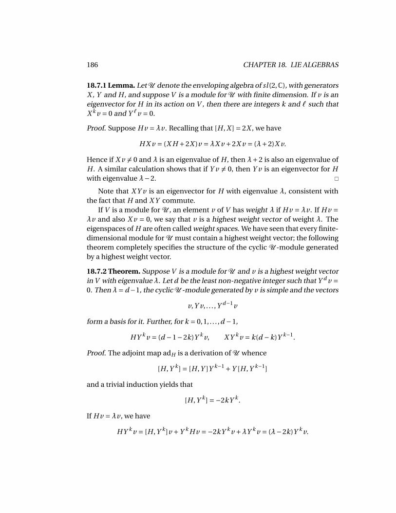
186 CHAPTER 18. LIE ALGEBRAS
18.7.1 Lemma. Let U denote the enveloping algebra of sl (2,C), with generatorsX , Y and H , and suppose V is a module for U with finite dimension. If v is aneigenvector for H in its action on V , then there are integers k and ` such thatX k v = 0 and Y `v = 0.
Proof. Suppose H v =λv . Recalling that [H , X ] = 2X , we have
H X v = (X H +2X )v =λX v +2X v = (λ+2)X v.
Hence if X v 6= 0 and λ is an eigenvalue of H , then λ+2 is also an eigenvalue ofH . A similar calculation shows that if Y v 6= 0, then Y v is an eigenvector for Hwith eigenvalue λ−2.
Note that X Y v is an eigenvector for H with eigenvalue λ, consistent withthe fact that H and X Y commute.
If V is a module for U , an element v of V has weight λ if H v = λv . If H v =λv and also X v = 0, we say that v is a highest weight vector of weight λ. Theeigenspaces of H are often called weight spaces. We have seen that every finite-dimensional module for U must contain a highest weight vector; the followingtheorem completely specifies the structure of the cyclic U -module generatedby a highest weight vector.
18.7.2 Theorem. Suppose V is a module for U and v is a highest weight vectorin V with eigenvalue λ. Let d be the least non-negative integer such that Y d v =0. Then λ= d−1, the cyclic U -module generated by v is simple and the vectors
v,Y v, . . . ,Y d−1v
form a basis for it. Further, for k = 0,1, . . . ,d −1,
HY k v = (d −1−2k)Y k v, X Y k v = k(d −k)Y k−1.
Proof. The adjoint map adH is a derivation of U whence
[H ,Y k ] = [H ,Y ]Y k−1 +Y [H ,Y k−1]
and a trivial induction yields that
[H ,Y k ] =−2kY k .
If H v =λv , we have
HY k v = [H ,Y k ]v +Y k H v =−2kY k v +λY k v = (λ−2k)Y k v.
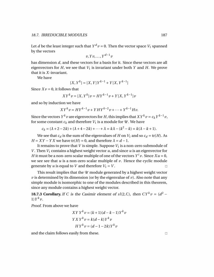
18.7. IRREDUCIBLE MODULES 187
Let d be the least integer such that Y d v = 0. Then the vector space V1 spannedby the vectors
v,Y v, . . . ,Y d−1v
has dimension d , and these vectors for a basis for it. Since these vectors are alleigenvectors for H , we see that V1 is invariant under both Y and H . We provethat it is X -invariant.
We have[X ,Y k ] = [X ,Y ]Y k−1 +Y [X ,Y k−1]
Since X v = 0, it follows that
X Y k v = [X ,Y k ]v = HY k−1v +Y [X ,Y k−1]v
and so by induction we have
X Y k v = HY k−1v +Y HY k−2v +·· ·+Y k−1H v.
Since the vectors Y k v are eigenvectors for H , this implies that X Y k v = ck Y k−1v ,for some constant ck and therefore V1 is a module for U . We have
ck = (λ+2−2k)+ (λ+4−2k)+·· ·+λ= kλ− (k2 −k) = k(λ−k +1).
We see that cd is the sum of the eigenvalues of H on V1 and so cd = tr(H). AsH = X Y −Y X we have tr(H) = 0, and therefore λ= d −1.
It remains to prove that V is simple. Suppose V1 is a non-zero submodule ofV . Then V1 contains a highest weight vector u, and since u is an eigenvector forH it must be a non-zero scalar multiple of one of the vectors Y i v . Since X u = 0,we see see that u is a non-zero scalar multiple of v . Hence the cyclic modulegenerate by u is equal to V and therefore V1 =V .
This result implies that the U module generated by a highest weight vectorv is determined by its dimension (or by the eigenvalue of v). Also note that anysimple module is isomorphic to one of the modules described in this theorem,since any module contains a highest weight vector.
18.7.3 Corollary. If C is the Casimir element of sl (2,C), then C Y k v = (d 2 −1)Y k v .
Proof. From above we have
X Y Y k v = (k +1)(d −k −1)Y k v
Y X Y k v = k(d −k)Y k v
H Y k v = (d −1−2k)Y k v
and the claim follows easily from these.
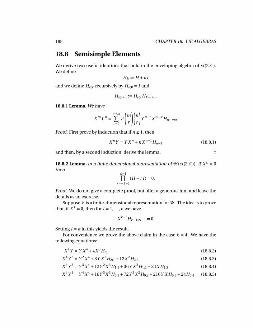
188 CHAPTER 18. LIE ALGEBRAS
18.8 Semisimple Elements
We derive two useful identities that hold in the enveloping algebra of sl (2,C).We define
Hk := H +kI
and we define Hk;r recursively by Hk;0 = I and
Hk;i+1 := Hk;i Hk−i+1.
18.8.1 Lemma. We have
X mY n =m∧n∑r=0
r !
(m
r
)(n
r
)Y n−r X m−r Hn−m;r
Proof. First prove by induction that if n ≥ 1, then
X nY = Y X n +nX n−1Hn−1 (18.8.1)
and then, by a second induction, derive the lemma.
18.8.2 Lemma. In a finite dimensional representation of U (sl (2,C)), if X k = 0then
k−1∏r=−k+1
(H − r I ) = 0.
Proof. We do not give a complete proof, but offer a generous hint and leave thedetails as an exercise.
Suppose V is a finite-dimensional representation for U . The idea is to provethat, if X k = 0, then for i = 1, . . . ,k we have
X k−i Hk−1;2i−1 = 0.
Setting i = k in this yields the result.For convenience we prove the above claim in the case k = 4. We have the
following equations:
X 4Y = Y X 4 +4X 3H3;1 (18.8.2)
X 4Y 2 = Y 2X 4 +8Y X 3H2;1 +12X 2H2;2 (18.8.3)
X 4Y 3 = Y 3X 4 +12Y 2X 3H1;1 +36Y X 2H1;2 +24X H1;3 (18.8.4)
X 4Y 4 = Y 4X 4 +16Y 3X 3H0;1 +72Y 2X 2H0;2 +216Y X H0;3 +24H0;4 (18.8.5)
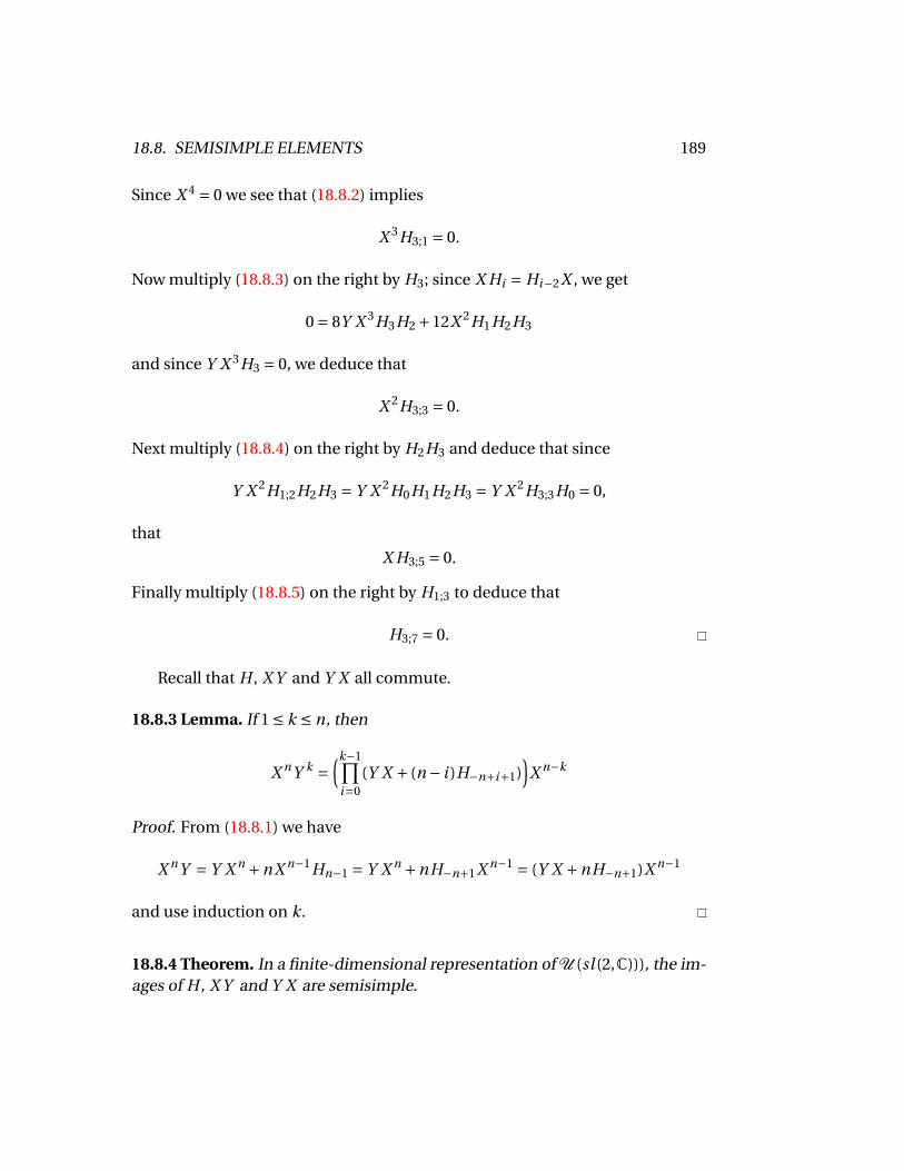
18.8. SEMISIMPLE ELEMENTS 189
Since X 4 = 0 we see that (18.8.2) implies
X 3H3;1 = 0.
Now multiply (18.8.3) on the right by H3; since X Hi = Hi−2X , we get
0 = 8Y X 3H3H2 +12X 2H1H2H3
and since Y X 3H3 = 0, we deduce that
X 2H3;3 = 0.
Next multiply (18.8.4) on the right by H2H3 and deduce that since
Y X 2H1;2H2H3 = Y X 2H0H1H2H3 = Y X 2H3;3H0 = 0,
that
X H3;5 = 0.
Finally multiply (18.8.5) on the right by H1;3 to deduce that
H3;7 = 0.
Recall that H , X Y and Y X all commute.
18.8.3 Lemma. If 1 ≤ k ≤ n, then
X nY k =(k−1∏
i=0(Y X + (n − i )H−n+i+1)
)X n−k
Proof. From (18.8.1) we have
X nY = Y X n +nX n−1Hn−1 = Y X n +nH−n+1X n−1 = (Y X +nH−n+1)X n−1
and use induction on k.
18.8.4 Theorem. In a finite-dimensional representation of U (sl (2,C))), the im-ages of H , X Y and Y X are semisimple.
190 CHAPTER 18. LIE ALGEBRAS
Proof. Since H and X Y commute and Y X = X Y −H , it is enough to show thatH and Y X are semisimple. By Lemma 18.7.1, there is an integer k such thatX k = 0. From Lemma 18.8.2 it follows that H is semimple, and so the underlyingvector space V is a direct sum of eigenspaces of H . Suppose Vλ is one of theseeigenspaces, where λ is the eigenvalue of H .
By Lemma 18.8.3 we have
0 = X k Y k = (Y X +k(H − (k −1)I ) · · · (Y X +H)
and if z ∈Vλ, then
0 = (Y X +k(λ− (k −1)I ) · · · (Y X +λ)z.
Hence the minimal polynomial of Y X on Vλ has only simple zeros, and there-fore Y X is semisimple on Vλ. We conclude that Y X must be semisimple.
18.9 Semisimple Modules
18.9.1 Theorem. Any finite dimensional module for U (sl (2,C)) is semisimple.
Proof. Let U denote U (sl (2,C)), let M be a finite-dimensional U -module, andlet C be the Casimir element of U . Since C is central and semisimple, M is thedirect sum of eigenspaces of C , and so to prove the theorem it will suffice if weshow that any eigenspace for C semisimple.
Hence we assume that M itself is an eigenspace for C . Since H also is semisim-ple, M is the direct sum of weight spaces Mσ and, if N ≤ M , then N is the directsum of its weight space Nσ, where
Nσ = N ∩Mσ.
We havedim(Mσ) = dim(Nσ)+dim(Mσ/Nσ).
Note that M/N is a U -module and
(M/N )σ = Mσ/Nσ.
Next assume we have the composition series for M :
0 = M0 < M1 < ·· · < Mr = M .
18.9. SEMISIMPLE MODULES 191
Then
dim(Mσ) =r∑
i=1dim(Mi /Mi−1)σ
but Mi /Mi−1 is a simple U -module and consequently dim(Mi /Mi−1)σ = 1. Weconclude that dim(Mσ) = r and that dim(M) is r times the number of eigen-values of H . The cyclic U -submodule of M generated by a non-zero elementis simple and, since all non-zero elements of M are eigenvectors for C with thesame eigenvalue, all these simple modules have the same dimension.
Choose a basis x1, . . . , xd for M . Then
M = x1U +·· ·+xdU .
where each submodule xi U contains a simple submodule Si (say). (We do notassume that this is a direct sum.) Since dim(Mσ) = r , we have d = r . Sincex1, . . . , xr is a basis, the sum
S1 +·· ·+Sr
is direct and therefore dim(M) is bounded below by r times the number ofeigenvalues of H . But we saw that equality holds, and therefore M is a directsum of simple modules as required.
This proof follows Jantzen [?].
192 CHAPTER 18. LIE ALGEBRAS
Chapter 19
Terwilliger Algebras
Let A be an association scheme with d classes and let π be an equitable parti-tion of its vertex set with e classes. Define the diagonal 01-matrix Fi by setting(Fi )u,u = 1 if u lies in the i -th class of π. Then the matrices Fi are symmetricidempotents and ∑
iFi = I .
We will study the algebra generated by A together with the matrices Fi .If u is a vertex in the scheme and the i -th cell of π consists of the vertices
x such that (u, x) lies in the i -th relation, the algebra we get is the Terwilligeralgebra of the scheme relative to the vertex u.
19.1 Modules
Our basic task is to determine the irreducible modules of the Terwilliger alge-bra. Suppose A is an association scheme with d classes A0, . . . , Ad and vertexset V , and assume |V | = v . Let T denote the Terwilliger algebra of this schemeand suppose W is an irreducible T-module. Since W is invariant under A , itmust have basis that consists of eigenvectors for A . Similarly it must have basisthat consists of eigenvectors for the matrices Fi , that is, vectors whose supportsare subsets of the cells of the partition π.
The subspace spanned by the characteristic vectors of the cells of π is T-invariant and has dimension equal to |π|, the number of cells of π. We call it thestandard module It is a cyclic T-module, generated by 1. You may prove that itis irreducible.
193
194 CHAPTER 19. TERWILLIGER ALGEBRAS
This may seem an encouraging start to determining the irreducible mod-ules for the Terwilliger algebra, but unfortunately further progress will requiremuch more effort. Since T is transpose-closed, Rv decomposes into an orthog-onal sum of irreducible T-modules. Hence if W is irreducible and is not thestandard module, we may assume that it is orthogonal to it. Thus each elementof W will be orthogonal to the vectors Fi 1—it sums to zero on the cells of π.
19.1.1 Lemma. If W is an irreducible module for an algebra B and f is an idem-potent in B, then W f is an irreducible module for f B f .
Proof. We may assume dim(W ) ≥ 2, or there is nothing to prove. Since
W f f B f =W f B f ≤W f ,
we see that W f is a module for f B f .
Suppose U is an f B f -submodule of W f . Each element of U can be writtenas w f where w ∈ W and as f 2 = f , it follows that U f =U . Since U f B is a B-submodule of W , it is either zero or equal to W . If it is equal to W , then
U =U f B f =W f
and therefore W f is irreducible for f B f .
To complete the proof, we show that U f B cannot be zero. The key is tonote that the set
u ∈W : uB = 0
is a B-submodule of W . Since W is simple and not zero, it follows that this setmust be the zero module. Consequently U f B cannot be zero.
Note that f B f is a subspace of B and is closed under multiplication, butfails to be a subalgebra because it does not contain I (in general). However
f B f + (I − f )B(I − f )
is a subalgebra of B.
When we want to use Lemma 19.1.1, we will have two possible sources ofidempotents: the matrices Fi and the principal matrix idempotents E j .
19.2. THINNESS 195
19.2 Thinness
Let T be the Terwilliger algebra for an association scheme A and let W be aT-submodule of Rv . We say that W is thin if for each i we have
dim(Fi W ) ≤ 1.
We also say that W is dual thin if for each j ,
dim(E j W ) ≤ 1.
We generalise the concept of thinness. Suppose B is an algebra. We say that aset of idempotents F1, . . . ,Fr is a resolution of the identity if they are pairwiseorthogonal (Fi F j = 0 when i 6= j ) and∑
iFi = I .
A module W for B is thin relative to the resolution F1, . . . ,Fr if dim(Fi W ) ≤ 1for all i .
Being thin is not easy, but it is a desirable property that holds in many inter-esting cases.
19.2.1 Lemma. If A is an association scheme then the standard modules arethin and dual thin,
Proof. Exercise.
19.2.2 Theorem. If the algebra B is self-adjoint, then it is thin relative to theresolution F1, . . . ,Fr if and only if the subalgebra
F1BF1 +·· ·+Fr BFr
is commutative.
19.2.3 Lemma. Suppose T is the Terwilliger algebra of an association schemerelative to some vertex. If each matrix in
F0TF0 +·· ·+FeTFe
is symmetric, or if Aut(X )1 is generously transitive on each cell of π, then T isthin.
Proof. For the first, two symmetric matrices commute if and only if their prod-uct is symmetric. The second condition implies that each FiTFi is the Bose-Mesner algebra of a symmetric association scheme.
196 CHAPTER 19. TERWILLIGER ALGEBRAS
19.3 Jaeger Algebras
We define some endomorphisms of Matv×v (C). If A is a v × v matrix define theoperators X A and YA on Matv×v (C) by
X A(M) := AM , YA(M) = M A∗
and if B is a v × v matrix, then we define ∆B by
∆B (M) := B M .
Note that
YA(YB (M)) = MB∗A∗ = M(AB)∗ = YAB (M),
which explains the A∗ in the definition of YA. Also X A and YB commute, for anyA and B .
If A is an association scheme, we define J2 to be the algebra generated bythe matrices X A for A in C[A ]. We define J3(A ) to be the algebra generated bythe operators
X A, ∆B , A,B ∈C[A ].
We obtain J4(A ) by adjoining the right multiplication operators YA as wellThe vector space Matv×v (C) is a module M for J3, and the subspace of ma-
trices with all but the i -th column zero is a submodule, which we denote byM(i ). We see that M is the direct sum of the modules M(i ).
Our first result shows that J3(A ) is a kind of global Terwilliger algebra.
19.3.1 Lemma. The algebra generated by the restriction to M(i ) of the oper-ators in J3 is isomorphic to the Terwilliger algebra of A relative to the i -thvertex.
Proof. We have
X A(ei eTj ) = (Aei )eT
j
and
∆B (ei eTj ) = (Bi , j ei )eT
j .
So X A is represented on M( j ) by the matrix A, and ∆B by the diagonal matrixformed from the vector Be j .
19.3. JAEGER ALGEBRAS 197
We say that a J3-submodule U of Matv×v (C) is thin if the subspaces ∆Ai
are 1-dimensional, and say that it is dual thin if the subspaces XE j U are 1-dimensional.
19.3.2 Lemma. If A is metric then a thin submodule of Matv×v (C) is dual thin,if A is cometric then a dual thin submodule of Matv×v (C) is thin.
Proof. Suppose A is metric relative to the Schur idempotent A1. If C is a v × vmatrix, then
(A1(Ai C )) A j = 0
if |i − j | > 1. Hence if M is submodule of Matv×v (C), then
A1(Ai M) ≤ Ai−1 M + Ai M + Ai+1 M . (19.3.1)
Now let r denote the least positive integer such that Ar M 6= 0, and let d bethe greatest positive integer such that Ar+d−1 M 6= 0. From (19.3.1) it followsthat if r ≤ i ≤ r +d −1 then Ai M 6= 0. We also see that M is generated by thesubspace Ad M as an X A1 -module. In other terms,
M = ⟨A1⟩(Ad M).
If E j is a matrix idempotent, then
E j M = E j ⟨A1⟩(Ar M) = E j (Ar M)
If M is thin, then dim(Ar M) = 1 and therefore dim(E j M) ≤ 1 for all j .Therefore M is dual thin.
Suppose A is cometric relative to E1 and let s be the least integer such thatEs M 6= 0. Then each column of a matrix in E j M lies in col(E j ), and so if C ∈ M ,then each column of E1 (Ei M) is the Schur product of a column of E1 with avector in col(Ei ). Hence by ??? we have
E1 (Ei M) ≤ Ei−1M +Ei M +Ei+1M .
Given this, it is easy to prove the second part of the theorem.
198 CHAPTER 19. TERWILLIGER ALGEBRAS
Chapter 20
Strongly Regular Graphs
20.1 Strongly Regular Graphs
We apply the theory at hand to strongly regular graphs. Assume X is stronglyregular with adjacency matrix A, and suppose that A has the partitioned form
A =0 1T 0
1 B1 N T
0 N B2
Thus B1 is the adjacency matrix of the neighborhood of the vertex 1 in X , andB2 is the adjacency matrix of the subgraph induced by the vertices at distancetwo from 1.
20.1.1 Theorem. If X is a strongly regular graph and T is its Terwilliger algebrarelative to some vertex, then an irrreducibleT-module lies in one of the follow-ing classes:
(a) The standard module, with dimension three.
(b) Modules with dimension two, parameterized by eigenvectors w of B1 suchthat N w is an eigenvector for B2.
(c) Modules with dimension one, arising from an eigenvector of B1 in ker(N T )or from an eigenvector of B2 in ker(N ). Each of these modules is an eigenspacefor A.
199
200 CHAPTER 20. STRONGLY REGULAR GRAPHS
Proof. Suppose W is an irreducible T-module. We assume that W is not thestandard module, and hence it lies in the orthogonal complement to the stan-dard module. In particular F0W = 0.
First we consider the case where F1W = 0. In this case if x ∈W , then supp(x)is a subset of the vertices at distance two from 1. Since0 1T 0
1 B1 N T
0 N B2
00w
= 0
N T wB2w
we conclude that if
x = 0
0w
∈W,
then N T w = 0 and 00
B2w
∈W.
Since the span W2 of the vectors B r2 w is B2-invariant and since B2 is symmetric,
there is an eigenvector v for B2 contained in W2. Hence the vector00v
spans a 1-dimensional T-invariant subspace.
Similarly if F2W E = 0, then dim(W ) = 1, and W is spanned by an eigenvec-tor for B1 that lies in ker(N ).
So we assume that neither F1W nor F2W are zero. If
x =0
uv
∈W,
then 0u0
= F1x ∈W
20.1. STRONGLY REGULAR GRAPHS 201
and so
A
0u0
= 0
B1uNu
∈W.
Accordingly the vectors 0B r
1 u0
all lie in W and so there is an eigenvector w for B1 such that
z := 0
w0
∈W.
If we assume that B1w =λw , then
Az = A
0w0
= 0λwN w
∈W
The matrices I , A and J form a basis for the algebra of polynomials in A, and sothe vectors
z, Az, J z
span the cyclic A-module generated by z. Since J z = 0, this module is spannedby z and Az. It follows that that the span of z and Az contains an eigenvectorfor A, necessarily of the form 0
wβN w
,
for some scalar β. If the eigenvalue for this eigenvector is θ, then
θ
0w
βN w
= A
0w
βN w
= 0
B1w +βN T N wN w +βB2N w
= 0λw +βN T N wN w +βB2N w
whence we see that w is an eigenvector for N T N and N w is an eigenvector forB2. Consequently the span of the vectors 0
w0
,
00
N w
202 CHAPTER 20. STRONGLY REGULAR GRAPHS
is T-invariant; since these vectors are contained in W and since W is irre-ducible, they must be a basis for W .
20.1.2 Corollary. The Terwilliger algebra of a strongly regular graph is thin anddual thin.
Proof. It follows from our work above that an irreducible T-module is thin Weprove that an irreducible T-module is dual thin. Cases (a) and (c) are easy, sowe turn to case (b). Suppose w 6= 0 and
x = 0
w0
∈W.
Then E0x = 0. If E1x = 0, then x = E2x and so x is an eigenvector for A and thusgenerates a proper submodule of W . We conclude that neither E1x nor E2x canbe zero, and hence W is dual thin.
20.2 Local Eigenvalues
We apply the theory built up in the previous section to get information aboutlocal eigenvalues of strongly regular graphs.
Assume X is a strongly regular graph with parameters (v,k, a,c) and adja-cency matrix partitioned as in the previous section. We assume that the eigen-values of X are
k, θ, τ
where θ ≥ 0 and τ< 0. We denote the multiplicities of θ and τ by m(θ) and m(τ).We use δ to denote a − c and recall that
A2 = δA+ (k − c)I + c J .
Since T is thin, the matrices
F1 AF1, F1 AF2 AF1
commute and therefore the matrices
B1, N T N
20.2. LOCAL EIGENVALUES 203
also commute. Hence we can decompose each eigenspace of B1 into the sub-space of eigenvectors in ker(N T N ) and the subspace of eigenvectors orthog-onal to ker(N T N ) or, equivalently, eigenvectors in ker N and eigenvectors incol(N T )).
If w is an eigenvector for B in ker(N ) then 0w0
is an eigenvector for A (with eigenvalue θ or τ) and spans a 1-dimensional irre-ducible T-module.
Now suppose w is an eigenvector for B1 with eigenvalue λ in 1⊥∩ ker(N ).We have
F2 A2F1 = N B1 +B2N = δN + c J
and consequently
δN w = (δN + c J )w = (N B1 +B2N )w = (λI +B2)N w.
Therefore N w is an eigenvector for B2 with eigenvalue δ−λ, and the vectors 0w0
,
00
N w
span an irreducible T-module with dimension two. It is possible to show ina similar fashion that if z is an eigenvector for B2 with eigenvalue µ in 1⊥ ∩ker(N T ), then
B1N T z = (δ−µ)N T z
and the vectors 0N T z
0
,
00z
span an irreducible T-module with dimension two.
We note one further constraint. Since
F1 A2F1 = J +B 21 +N T N = δB1 + (k − c)I + c J
we haveB 2
1 −δB1 − (k − c)I =−N T N + (c −1)J
204 CHAPTER 20. STRONGLY REGULAR GRAPHS
and so if B w =λw and J w = 0, then
(λ2 −δλ− (k − c)) =−N T N w.
Thus w is an eigenvalue for N T N , and since this matrix is positive semidefinite,it follows that
λ2 −δλ− (k − c) ≤ 0,
or equivalently thatτ≤λ≤ θ.
For later use, note that
t 2 −δt − (k − c) = (t −θ)(t −τ).
A local eigenvalue of a strongly regular graph s an eigenvalue of B1 or B2 notequal to θ or τ.
20.2.1 Lemma. If X is a triangle-free strongly regular graph with parameters(v,k;0,c), then the eigenvalues of B2 are its valency k − c and a subset of θ, τand −c.
It follows that the second neighborhood of a vertex in a triangle-free stronglyregular graph is walk regular.
20.3 Dimensions
We determine the dimension of the Terwilliger algebra of a strongly regulargraph. Most the work has already been done, the main task left is to determinethe isomorphism classes of the irreducible T-modules.
We deal with the easy cases first. The standard module is the only modulewith dimension three, and so nothing more need to be said. Two 1-dimensionalmodules U and V are isomorphic if either both F1U and F1V are non-zero, orboth F2U and F2V are non-zero.
So consider the 2-dimensional T-module spanned by the vectors 0w0
,
00
N w
20.3. DIMENSIONS 205
where B1w =λw . Relative to this basis, F1 and F2 are represented by the matri-ces (
1 00 0
),
(0 00 1
).
We have
A
0w0
= 0λwN w
and
A
00
N w
= 0
N N T N wB2NW
= 0−(λ−θ)(λ−τ)w
(δ−λ)N w
.
and therefore the matrix representing A is(λ −(λ−θ)(λ−τ)1 δ−λ
).
It follows that this module is determined by the eigenvalue λ. We also see thatthe structure of the Terwilliger algebra is determined by the eigenvalues of Xand the eigenvalues of its first and second neighborhoods.
20.3.1 Theorem. Let X be a strongly regular graph with v vertices. Let s denotethe sum of the number of eigenvalues of B1 in θ,τ plus and the number ofeigenvalues of B2 in θ,τ, and let r denote the number of eigenvalues of B1 notin this set. Then dim(T) = 9+4r + s and dim(Z (T)) = 1+ r + s.
It is clear that 0 ≤ s ≤ 4 but in fact s must be positive if X is not a conferencegraph. For
k +`= mθ+mτ
and if k > ` and mθ > mτ, then A has an eigenvector with eigenvalue θ sup-ported on the neighborhood of a vertex. Similar conclusions hold if we reverseone or both of these inequalities.
By way of example we consider the strongly regular graph L(Kn), where n ≥5. Its parameters are ((
n
2
),2n −4;n −2,4
)and its eigenvalues are
2n −4, n −4, −2.
206 CHAPTER 20. STRONGLY REGULAR GRAPHS
The neighborhood of a vertex is isomorphic to K2 äKn−2, whence its eigenval-ues are
n −2, n −4, 0, −2
and the second neighborhood is isomorphic to L(Kn−2), with eigenvalues
2n −8, n −6, −2.
Thus there are two non-local eigenvalues in the neighborhood, one non-localeigenvalue in the second neighborhood and one local eigenvalue. It followsthat the Terwilliger algebra has dimension
9+3+4 = 16
while its centre has dimension five.
Chapter 21
Hamming Schemes
21.1 The Binary Hamming Scheme
The Hamming scheme H(d ,2) is a metric and cometric association scheme.The matrix A = A1 is the adjacency matrix of the d-cube, and its eigenvaluesare the integers
d −2i , i = 0, . . . ,d
with respective multiplicities (d
i
).
The automorphism group of the Hamming scheme is vertex-transitive, and sothe Terwilliger algebra is the same for each vertex.
We can writeA = R +L
where L = RT and R is the natural raising operator on the lattice of subsets of1, . . . ,d. (So L is the natural lowering operator.)
21.1.1 Theorem. The Terwilliger algebra of the binary Hamming scheme is aquotient of the enveloping algebra U (sl (2,C)).
Proof. View the vertices of the Hamming scheme as subsets of 1, . . . ,d. Define
H = RL−LR.
We note thatRα,β = 1
207
208 CHAPTER 21. HAMMING SCHEMES
if and only if α ⊆ β and |β| = |α| + 1. Further Hα,β = 0 if |α| 6= |β| and, if |α| =|β| = i , then
Hα,β = d −2i .
It follows that
H =d∑
i=0(d −2i )Fi
and hence the the algebra of all polynomials in H is the equal to the algebragenerated by the diagonal matrices Fi .
Since[R,L] = H , [H ,R] = 2R, [H ,L] =−2L
the algebra generated by R, L and H is a homomorphic image of U (sl (2,C)).To complete the proof we must show that R and L generate the Terwilliger
algebra of H(n,d). But since the scheme is metric, each element of the Bose-Mesner algebra is a polynomial in A and since the algebra generated by H con-tains each Fi , we conclude that R and L generate the Terwilliger algebra.
21.2 Modules
With what we know about the representation theory of sl (2,C), it is easy to de-termine the irreducible T-modules for the binary Hamming scheme H(d ,2). Ifu is a vertex of H(d ,2) with Hamming weight i , then the vectors
v,Rv, . . . ,Rd−2i v
are a basis for an irreducible module of dimension d − 2i + 1. If u and v arebinary vectors then the irreducible modules they generate are isomorphic ifand only if u and v have the same Hamming weight.
21.2.1 Lemma. We have
dim(T(H(d ,2))) = 1
6(d +1)(d +2)(d +3).
Proof. If 0 ≤ 2i ≤ d , then our Terwilliger algebra has one isomorphism class ofirreducible module with dimension d −2i +1, whence
dim(T(H(d ,2))) = ∑i≤d/2
(d −2i +1)2 = 1
6(d +1)(d +2)(d +3).
21.2. MODULES 209
21.2.2 Lemma. The Terwilliger algebra of the Hamming scheme is thin and dualthin.
Proof. If v has Hamming weight i , then the Hamming weight of each vectorin supp(R j v) is i + j . Hence Fi+ j R j v = R j v , and therefore the R-module gen-erated by v is thin. Since the Hamming schemes are metric, it follows fromLemma 19.3.2 that this module is also dual thin.
210 CHAPTER 21. HAMMING SCHEMES
Chapter 22
Spin
22.1 Braids
The braid group on n strands Bn is the group generated by elements
σ1, . . . ,σn−1
subject to the relations:
σiσ j =σ jσi , if |i − j | ≥ 2
σiσ jσi =σ jσiσ j , if |i − j | = 1.
[braids, closure]The map that takes σi to the transposition (i i +1) in the symmetric group
Sym(n) extends to a homomorphism from Bn . (Its kernel consists of the purebraids.)
The Temperley-Lieb algebra T Ln(β) contains a homomorphic image of theBraid group.
22.2 Nomura Algebras
Let A and B be v × v matrices and suppose B is Schur invertible. The Nomuraalgebra NA,B consists of all v × v matrices for which all the vectors
Aei Be(−)
j
211
212 CHAPTER 22. SPIN
are eigenvectors. If M ∈ NA,B , we define ΘA,B (M) to be the v × v matrix withi j -entry equal to eigenvalue of M associated to Aei Be j . Thus I ∈ NA,B andΘA,B = J .
If M , N ∈NA,B , then
ΘA,B (M N ) =ΘA,B (M)ΘA,B (N ).
Thus NA,B is an algebra under matrix multiplication, and the image of NA,B
underΘA,B is an algebra under Schur multiplication. We note that
NA,B =NB ,A
whileΘB ,A(M) =ΘA,B (M)T .
22.2.1 Lemma. If A is invertible and B is Schur invertible, thenΘA,B is injectiveand NA,B is a commutative algebra.
A v × v matrix W is a type-II matrix if it is Schur invertible and
W W (−)T = v I .
Hadamard matrices provide one class of examples. If W is a type-II matrix, thenW is invertible and
W −1 = 1
vW (−)T .
22.2.2 Lemma. The matrix W is a type-II matrix if and only if J ∈NW,W (−) .
The Nomura algebra NW,W (−) will play an important role in our work and sowe will denote it by NW . We also writeΘW forΘW,W (−) .
22.3 Braids
Let A, B and C be v × v matrices. We define endomorphisms X A, ∆B and YC ofthe vector space Matn×n(C) by
X A(M) := AM , ∆B (M) := B M , YC (M) := MC T .
(We could instead use respectively A ⊗ I , DB and I ⊗C , where DB is a diagonalmatrix with the entries of B as its diagonal entries and all three matrices areviewed as elements of End(Matv×v (C)).)
22.4. JONES PAIRS 213
22.3.1 Lemma. Suppose A,B ∈ Matv×v (C). Then R ∈ NA,B and ΘA,B (R) = S ifand only
XR∆B X A =∆B X A∆S .
We see that A ∈NA,B andΘA,B (A) = B if and only if
X A∆B X A =∆B X A∆B ;
we call this the braid relation. [If A is invertible and B is Schur invertible andA ∈NA,B , does it follow thatΘA,B (A) = B?]
We note the following result, which we call the exchange identity.
22.3.2 Theorem. Let A, B , C , Q, R, S be v × v matrices. Then
X A∆B XC =∆Q XR∆S
if and only ifX A∆C XB =∆R XQ∆ST .
Proof. Apply each of the four products to the matrix ei eTj .
The bilinear form tr(M N T ) on Matv×v (C) is non-degenerate and hence al-lows to define the adjoint of elements of End(Matv×v (C)). We denote the adjointby transpose and observe that
(X A)T = X AT , (∆B )T ) =∆B .
Thus the braid relation implies that
X AT∆B X AT =∆B X AT∆B .
22.4 Jones Pairs
We say that v×v matrices A and B form a one-sided Jones pair if A is invertible,B is Schur invertible and A ∈ NA,B . They form a Jones pair if (A,B T ) is also aone-sided Jones pair.
22.4.1 Lemma. If (A,B) is a one-sided Jones pair, so are each of the following:
(a) (AT ,B).
214 CHAPTER 22. SPIN
(b) (A−1,B (−)).
(c) (D−1 AD,B), where D is diagonal and invertible.
(d) (A,BP ), where P is a permutation matrix.
(e) (λA,λB), for any non-zero complex number λ.
22.4.2 Lemma. The matrices A and B form a one-sided Jones pair if and only iffor all i and j we have
A(Aei Be j ) = Bi , j (Aei Be j ).
22.4.3 Corollary. Let (A,B) be a pair of v×v matrices and let D j be the diagonalmatrix formed from the j -th column of B . Then (A,B) is a one-side Jones pairif and only if, for j = 1, . . . , v ,
AD j A = D j AD j .
22.4.4 Lemma. If (A,B) is a one-sided Jones pair, then each column of B sumsto tr(A).
Proof. From the previous result we have
A−1D j A = D j AD−1j
whence A and D j are similar and tr(A) = tr(D j ). Therefore each column of Bsums to tr(A).
We say a Jones pair (A,B) is invertible if A is Schur invertible and B is in-vertible.
22.4.5 Theorem. Suppose (A,B) is a one-sided Jones pair and B is invertible,then A and B are type-II matrices and the diagonal of A is constant.
Proof. If A ∈NA,B then A−1 ∈NA,B and so
ΘB ,A(A−1) = B (−)T .
This implies thatX A−1∆A XB =∆A XB∆B (−)T (22.4.1)
22.4. JONES PAIRS 215
and taking the transpose of this, we get
XB T∆A X A−T =∆B (−)T XB T∆A.
If we apply the right side to I we get B T (A A−T ), if we apply the left side to Ithe result is
B (−)T (B T (A I )) = J (A I )
and henceB T (A A−T ) = J (A I ).
Since B is invertible and its row sums are all equal t some constant β, this im-plies that
A A−T = B−T J (A I ) =βJ (A I ).
The sum of the entries in the i -th column of A A−T is∑r
(A−1)r,i (AT )r,i =∑
r(A−1)r,i Ai ,r = 1
and therefore all columns of J (A I ) must be equal. It follows that v A A−T = Jand so A is a type-II matrix with constant diagonal.
To complete the proof we multiply each side of (22.4.1) on the left by ∆A(−)
and on the right by XB−1 to obtain
∆A(−) X A−1∆A = XB∆B (−)T XB−1 .
Taking inverses on both sides yields
∆A(−) X A∆A = XB∆B T XB−1
and applying each side to I gives
A(−) (A(A I )) = B(B T B−1).
Since the diagonal of A is constant, the left side here is equal to a J for some aand so
B T B−1 = aB−1 J
Arguing as before, the sum of a row of B T B−1 is 1. Therefore B−1 J is a multipleof J ; from this we see that B is a type-II matrix.
216 CHAPTER 22. SPIN
22.4.6 Lemma. If (A,B) is Jones pair and A is Schur invertible, then B is invert-ible.
Proof. Apply both sides of (22.4.1) to J ; this yields
A−1(A (B J )) = A (BB (−)T ).
Since (A,B T ) is a Jones pair the row sums of B equal tr(A) and so the left sidehere is equal to tr(A)I . As A is Schur invertible it follows that BB (−)T is diagonal.However the diagonal entries of BB (−)T are all equal and so it is a scalar matrix.We conclude that B is type II and invertible.
22.5 Gauge Equivalence
If D is an invertible diagonal matrix we say that D−1 JD is a dual permutationmatrix. The Schur inverse of a dual permutation matrix is a dual permutationmatrix.
22.5.1 Lemma. If A, C and M are Schur invertible and X A∆M = ∆M XC , thenC (−) A is a dual permutation matrix. If B , C and M are invertible and ∆B XM =XM∆C , then C B−1 is a permutation matrix.
22.5.2 Corollary. If (A,B) and (C ,B) are one-sided Jones pairs, then C = D−1 ADwhere D is invertible and diagonal.
22.5.3 Corollary. If (A,B) and (A,C ) are one-sided Jones pairs, then C = BPwhere P is a permutation matrix.
22.6 Nomura Algebras of Type-II matrices
A type-II matrix W is called a spin model if (W,W (−)) is a Jones pair. If W ∈NW ,then (W,W (−)) need not be a Jones pair, because the columns of W (−) might notsum to tr(A). If σ denotes the sum of a column of W (−) and we choose γ so that
γ2 tr(W ) =σ
then γW is a spin model.
22.6. NOMURA ALGEBRAS OF TYPE-II MATRICES 217
22.6.1 Theorem. Let A be a v×v type-II matrix. ThenΘA is a bijection from NA
to NAT and ΘAT is a bijection from NAT to NA. If R ∈ NA then ΘAT (ΘA(R)) =vRT .
Proof. Suppose R ∈NA andΘA(R) = S. Then
XR∆A(−) X A =∆A(−) X A∆S
and the transpose of this is
X AT∆A(−) XRT =∆S X AT∆A(−)
and applying the exchange identity to this yields
X AT∆RT X A(−) =∆AT XS∆A(−)T .
If we multiply both sides of this on the left by ∆A(−)T and on the right by X A(−)−1
we getXS∆A(−)T X A(−)−1 =∆A(−)T X AT∆RT .
Since A(−)−1 = 1v AT , this yields
XS∆A(−)T X AT =∆A(−)T X AT∆vRT
whence S ∈NAT andΘAT (S) = vRT .AsΘAT (ΘA(R)) = vRT , we see thatΘA andΘAT are bijections.
This proof shows that the composite map
1
vΘATΘA
is the transpose map on NA. Hence 1vΘAΘAT is the transpose map on NAT . In
factΘA andΘAT commute with the transpose.
22.6.2 Corollary. If A is a type-II matrix and R ∈NA, then RT ∈NA andΘA(RT ) =ΘA(R)T .
Proof. If R ∈NA then vRT =ΘAT (ΘA(R) ∈NA and
ΘA(vRT ) =ΘA(ΘAT (ΘA(R))) = vΘA(R)T .
218 CHAPTER 22. SPIN
22.6.3 Corollary. If A is a v × v type-II matrix and M , N ∈NA, then
ΘA(M N ) = 1
vΘA(M)Θ(N ).
22.6.4 Corollary. If A is a type-II matrix then its Nomura algebra is closed un-der matrix multiplication, Schur multiplication, transpose and complex conju-gation.
Proof. We know that NA is closed under matrix multiplication and that
ΘA(M N ) =ΘA(M)ΘA(N ),
from which it follows that the image of ΘA is Schur-closed. Therefore NAT isSchur-closed. Swapping A and AT , we deduce that NA is Schur-closed.
We saw above that NA is closed under transpose. Since it is Schur-closed ithas a basis consisting of 01-matrices, and the complex span of these matricesis closed under complex conjugation.
This corollary asserts that NA is the Bose-Mesner algebra of an associationscheme.
22.7 Spin Models
By definition, W is a spin model if (W,W (−)) is a one-sided Jones pair.
22.7.1 Lemma. If A is a type-II matrix and (A, A(−)) is a one-sided Jones pair,then it is a Jones pair.
Proof. Since (A, A(−)) is a one-sided Jones pair, we have
X A∆A(−) X A =∆A(−) X A∆A(−)
and taking the transpose of this yields
X AT∆A(−) X AT =∆A(−) X AT∆A(−) .
Using the exchange identity we obtain
X AT∆AT X A(−) =∆AT X A(−)∆A(−)T
22.7. SPIN MODELS 219
and inverting both sides yields
X A(−)−1∆A(−)T X A−T =∆AT X A(−)−1∆A(−)T .
If we multiply on the left by ∆A(−)T and on the right by X AT , the result is
∆A(−)T X A(−)−1∆A(−)T = X A(−)−1∆A(−)T X AT .
We observe that A(−)−1 = 1v AT , whence the last equation yields
∆A(−)T X AT∆A(−)T = X AT∆A(−)T X AT
and therefore (AT , A(−)T ) is a one-sided Jones pair. From the transpose of thiswe see that (A, A(−)T ) is one-sided Jones pair, and thus it follows that (A, A(−)) isa Jones pair.
22.7.2 Theorem. If A is spin model, then NA =NAT andΘA =ΘAT .
Proof. We use gauge equivalence. If (A, A(−)) and A, A(−)T are one-sided Jonespairs, there is a permutation matrix P such that A(−)T = A(−)P , and conse-quently
NA,A(−)T =NA,A(−)P =NA,A(−)
Now A ∈NA if and only if
AT ∈NAT ,A(−) =NAT ,A(−)T .
Since NA is closed under transposes, the result holds.Suppose R ∈NA andΘA(R) = S then
XR∆A(−) X A =∆A(−) X A∆S
and if R ∈NAT andΘAT = T then
XR∆A(−)T X AT =∆A(−)T X AT∆T .
Consequently
(∆A(−)T X AT∆T )−1∆A(−) X A∆S = X A−T∆AT A(−) X A.
The left side here equals
∆T (−) X A−T∆AT∆A(−) X A∆S =∆T (−) (X A−T∆AT A(−) X A)∆S
220 CHAPTER 22. SPIN
If we defineΞ := X A−T∆AT A(−) X A
thenΞ∆S =∆TΞ. (22.7.1)
We compute Ξ(M), for any v × v matrix M . Note that
Ξ(M) = A−T (AT A−1 (AM))
Since (A, A(−)) and (AT , A(−)T ) are both one-sided Jones pairs, there is an invert-ible diagonal matrix C such that AT =C−1 AC . Therefore
AT A−1 = (C−1 AC ) A−1 =C−1 JC
and so
AT A−1 (AM) = (C−1 JC ) (AM) =C−1 AMC = AT C−1MC
and consequently
Ξ(M) = A−T (AT A−1 (AM)) =C−1MC .
Now apply each side of (22.7.1) to M ; we get
T (C−1MC ) =C−1(S M)C = S)C−1MC ).
We conclude that S = T .
Chapter 23
Abelian Spin
We study spin models in the Bose-Mesner algebras of abelian groups, aka trans-lation schemes.
23.1 Schemes
Suppose W is a type-II matrix. Its Nomura algebra is the Bose-Mesner algebraof an association scheme A ; thus NW =C[A ]. We assume A has d classes andtherefore dim(NW ) = d +1. Let E0, . . . ,Ed denote the principal idempotents ofthe scheme. Since E 2
i = Ei we see that ΘW (Ei ) must be a Schur idempotent inNW T and since
d∑i=0
Ei = I
we haved∑
i=0ΘW (Ei ) = J ,
whence it follows that the Schur idempotentsΘW (Ei ) are linearly independent.Thus they are the principal Schur idempotents of the scheme determined byW T .
A similar argument shows that if A0, . . . , Ad are the principal Schur idempo-tents of the scheme determined by W , then the matrices
1
vΘW (Ai )
are the principal idempotents of the scheme determined by W T .
221
222 CHAPTER 23. ABELIAN SPIN
Now we specialize to the case where W is a spin model. The eigenvaluespi ( j ) of the scheme are defined implicitly by
Ai =d∑
i=0pi ( j )E j .
Since NW = NW T , we see that ΘW maps C[A ] to itself and the matrix whichrepresents relative to the basis formed by E0, . . . ,Ed has i j -entry equal to p j (i ).It is traditionally denoted by P . It is invertible and we follow tradition furtherand set Q equal to vP−1. We have
E j = 1
v
d∑i=0
q j (i )Ai
where q j (i ) =Q j ,i . Since
ΘW T (Ai ) = vE Ti = vE i
we see that Q is the matrix that represents ΘW T relative to the basis A0, . . . , Ad .Therefore P−1QP is the matrix representing ΘW T relative to E0, . . . ,Ed . SinceNW T =NW , the operatorsΘW andΘW T commute. Therefore
Θ−1W ΘW TΘW =ΘW T
and therefore P−1QP =Q.
23.1.1 Theorem. If W is a spin model then P =Q.
Proof. We haveΘW =ΘW T .
23.2 Coordinate Matrices
Let W be a spin model, let A denote the associated set of principal Schur idem-potents and let E be the set of principal matrix idempotents. Since W ∈ NW ,there are scalars λ0, . . . ,λd (the eigenvalues of W ) such that
W =d∑
i=0λi Ei .
Let L be the diagonal matrix with Li ,i =λi . If M is an endomorphism of a vectorspace with basis β we use [M ]β to denote the matrix representing M relative toβ. Let T represent the transpose map.
23.2. COORDINATE MATRICES 223
23.2.1 Lemma. We have [XW ]E = L and [∆W ]A = L−1.
Proof. The first claim is immediate from the definition of the coefficients wi .For the the second note that
λi Ai =ΘW (W Ei ) =ΘW (W ) Ai =W (−) Ai
and consequentlyW (−) Ai =λi Ai
as required.
The last equation above implies that
W =d∑
i=0λ−1
i Ai .
Therefore
λr Er =W Er =d∑
i=0λ−1
i Ai Er =( d∑
i=0λ−1
i pi (r ))Er
and henceL1 = PL−11.
We see that diagonal matrices L such that L1 = P−11 correspond to the type-IImatrices in C[A ].
23.2.2 Lemma. We have [XW ]A = PLP−1 and [∆W ]E = P−1L−1P .
Proof. The matrix of eigenvalues P represents the change-of-basis map from E
to A and therefore[∆W ]E = P−1L−1P.
The second claim follows similarly.
The transpose map is an endomorphism of Matv×v (C) that maps NW toitself, which we denote by T . Both [T ]E and [T ]A are permutation matrices.Since
Θ(M T ) =Θ(M)T ,
we see that T andΘ commute, and consequently [T ]E = [T ]A . Note that
Θ2 = vT. (23.2.1)
224 CHAPTER 23. ABELIAN SPIN
23.3 Duality
Suppose W is a spin model and A is the corresponding association scheme.Then ΘW maps C[A ] to itself and swaps matrix with Schur multiplication. (IfA is the scheme of the cyclic group, then ΘW is better known as the discreteFourier transform.) We will derive various expressions forΘW .
We begin with the observation that W T ∈NW andΘW (W T ) =W (−)T . Hence
XW T∆W (−) XW =∆W (−) XW∆W (−)T (23.3.1)
Denote either side of this identity byΛ and note thatΛT =Λ.
23.3.1 Theorem. If R ∈NW andΘW (R) = S, thenΛ−1XRΛ=∆S andΛ−1∆STΛ=XR .
Proof. Since R commutes with W T , we have
Λ−1XRΛ= XW −1∆W XW −T XR XW T∆W (−) XW
= XW −1∆W XR∆W (−) XW
=∆S .
Next
Λ−1∆STΛ=∆W T XW −1∆W∆ST∆W (−) XW∆W (−)T
=∆W T XW −1∆ST XW∆W (−)T .
As R ∈NW T andΘW =ΘW T , we have
XR∆W −1 XW T =∆W −1 XW T∆S
and therefore by the exchange identity
XR∆W T XW −1 =∆W T XW −1∆ST .
It follows that
Λ−1∆STΛ= XR∆W T XW −1 XW∆W (−)T = XR .
23.3.2 Corollary. If R ∈NW , thenΛ−2XRΛ2 = XRT andΛ−2∆SΛ
2 =∆ST .
23.3. DUALITY 225
Proof. First∆S = (∆S)T = (Λ−1XRΛ)T =ΛXRTΛ−1
and thereforeΛ−2XRΛ
2 =Λ−1∆SΛ= XRT .
SecondΛ−2∆STΛ2 =Λ−1XRΛ=∆S
and so taking transposes we get
Λ2∆STΛ−2 =∆S ,
which yields our second claim.
You may also show that Λ−2XRTΛ2 = XR and Λ−2∆STΛ2 = ∆S , from whichwe get the following.
23.3.3 Corollary. If W is a spin model, then the mapΛ4 commutes with XR and∆S for all R,S in NW .
It is worth noting that we are dealing here with several algebras. First wehave Matv×v (C) and its subalgebra NW = C[A ], which is the Bose-Mesner al-gebra of A . Then inside the algebra End(Matv×v (C)) we have the algebra gen-erated by all operators
XR , ∆R , R ∈NW =NW T .
This may be viewed as an extended version of the Terwilliger algebra of A (andis not commutative). We will call it the Jaeger algebra and denote it by J3. Themap given by conjugation by Λ is an endomorphism of Matv×v (C) which fixesJ3.
Suppose (A,B) is a 1-sided Jones pair and define
K := X A∆B X A =∆B X A∆B .
ThenK 2 = (X A∆B X A)2 = (X A∆B )3
from which it follows thatΛ commutes with X A and ∆B . It is easy to verify that
K −1X AK =∆B
226 CHAPTER 23. ABELIAN SPIN
and consequently thatK −1∆B K = X A.
Specializing to the case where A is type II and B = A(−), we see that conjugationby K is a linear map that fixes the algebra generated by X A and ∆A(−) . This is, ingeneral, a subalgebra of the Jaeger algebra.
23.4 Modular Invariance
We combine the work from the previous two sections.
23.4.1 Lemma. If W is a spin model with δ = Wi ,i and M ∈ NW , then Θ(M) =vδΛ−1(M).
Proof. If R ∈NW andΘ(R) = S, thenΛ−1XRΛ=∆S and therefore
S =∆S(J ) =Λ−1XRΛ(J ).
HereΛ(J ) =∆W (−) XW∆W (−)T (J ) =∆W (−)W W (−)T = vW (−) I .
If δ :=Wi ,i , then it follows that
S =Λ−1XR (δv I ) = δvΛ−1(R).
The next result is known as the modular invariance property for the pair(P,L).
23.4.2 Theorem. Let W be a spin model with association scheme A and δ =Wi ,i , let P be the matrix of eigenvalues of A and let L be the diagonal matrix ofeigenvalues of W . Then (PL)3 = v
δ I .
Proof. From the previous lemma,
Θ= vδΛ−1vδXW T∆W (−) XW .
If F is the matrix that represents transpose, then we have
[XW ]E = L, [∆W (−) ]E = P−1LP, [XW T ]E = F LF.
Since [Θ]E = P , we haveP = vδF LF P−1LPL
23.5. THE CYCLIC GROUP 227
and so
I = vδ(P−1F )L(F P−1)LPL.
AsΘ2 = vT we have P 2 = vF and so
P−1F = F P−1 1
vP
from which we infer that
I = vδv−2(PL)3.
23.5 The Cyclic Group
The index set of the matrices in this section start at 0.Choose the complex number θ so that θ2 is a primitive v-th root of unity.
(Thus is v is odd then θ has order v , but if v is even then its order is 2v .) Definethe v × v matrix W by
Wi , j = θ(i− j )2.
Let S denote the diagonal matrix with Si ,i = θi 2. Then
θ(i− j )2 = θi 2θ−2i jθ j 2
and therefore if V is the Vandermonde matrix given by
Vi , j = (θ−2)i j
then
W = SV S.
23.5.1 Theorem. The matrix W is a spin model.
Proof. First
(W W (−)T )i , j =∑
rθ(i−r )2
θ−( j−r )2 = θi 2− j 2 ∑rθ2( j−i )r .
The last sum equal v if i = j and is otherwise zero. Therefore W W (−)T = v I andso W is a type-II matrix.
228 CHAPTER 23. ABELIAN SPIN
The matrix W lies in the Bose-Mesner algebra of the cyclic group of order v ,equivalently it is a circulant. If ζa is the column vector with i -entry θ2ai then ζa
is an eigenvector for all circulants of order v × v . Now
(W er W e(−)Ts )i = θ(i−r )2
θ−(i−s)2 = θr 2−s2θ−2i (r−s),
whenceW er W e(−)T
s = θr 2−s2ζr−s .
This implies that W ∈NW , and therefore we conclude that W is a spin model.

Bibliography
229
Index
R-clique, 25R-coclique, 25i -related, 2k-th symmetric power, 38
abelian, 177ad-nilpotent, 182adjoint map, 181algebra, 111algebra automorphism, 85American Math. Monthly, 151annihilator, 118antichain, 180association scheme, 1associative, 141
bent function, 75bilinear, 34bilinear forms scheme, 2Bose-Mesner algebra, 6braid group on n strands, 211braid relation, 213
cap, 62Casimir element, 183Cayley graph, 55central, 121character, 122character table, 108characters, 108classical parameters, 153
code, 59coherent algebra, 6, 168coherent configuration, 168cometric, 19commutant, 6commutator, 177commutator subalgebra, 178complement, 124composition series, 136coset graph, 59covering radius, 62cyclic, 118
degree, 25degree set, 25derivation, 178difference set, 76dimension, 59distance-regular graph, 17division algebra, 112doubly even, 71dual, 58, 74dual basis, 141dual code, 59dual degree, 25dual degree set, 25dual eigenvalues, 14dual permutation matrix, 216dual thin, 195, 197duality map, 63, 74
230
INDEX 231
eigenmatrix, 14eigenvalues, 13enveloping algebra, 112equivalent, 80even, 71exchange identity, 213extended code, 71
flat, 81formally dual, 74formally self-dual, 73Frame quotient, 22
generalized eigenvectors, 122generously transitive, 7Grassman scheme, 2
Hamming scheme, 2Hankel matrix, 160harmonic polynomial, 20Hecke algebra, 112highest weight vector, 186homogeneous, 169homomorphism, 181
ideal, 178idempotent, 119indecomposable, 120intersection matrices, 16, 21intersection numbers, 16invariant, 182invertible, 214irreducible, 108, 123
Jacobi identity, 177Jaeger algebra, 225Johnson scheme, 2Jones pair, 213
Killing form, 182
Krein parameters, 18Kronecker product, 33
length, 136level number, 179Lie algebra, 177Lie bracket, 177line digraph, 171local eigenvalue, 204locally distance regular, 166lowering operators, 180
main eigenvalues, 157metric, 17minimal polynomial of A relative to v ,
160modular invariance property, 226module, 181monomial matrix, 80multiplicities, 14
nilpotent, 120Nomura algebra, 211normal, 11normalized, 172
one-sided Jones pair, 213opposite, 116orthogonal, 7, 119
parallel class, 2partial spread, 2Peck poset, 180polynomial function, 20Potts models, 80primary decomposition, 122primitive, 120projective code, 60pseudocyclic, 41
232 INDEX
pure, 150pure braids, 211
quantum plane, 112quaternions, 113
radical, 127raising operator, 180rank, 59rank symmetric, 180ranked, 179regular module, 116representation, 181representation of Γ of degree d , 108resolution of the identity, 195root vectors, 122
Schur diameter, 18Schur inverse, 79self-dual, 74semisimple, 9, 124, 131simple, 117, 132Sperner, 180sphere-packing bound, 30spin model, 216split, 138standard module, 155, 193strongly regular, 15strongly Sperner, 180submodule, 181subscheme, 43symmetric, 2
Terwilliger algebra, 193thin, 195, 197thin relative to the resolution, 195trace, 141translation graph, 56type-II matrix, 79, 212
unimodal, 180universal enveloping algebra, 179
valencies, 14
weight, 64, 186weight enumerator, 68weight spaces, 186Weyl algebra, 112