DOCUMENT RESUME

ED 207 807 SE 035 500

AUTHOR Abelson, Harold; And OthersTITL3 Velocity Space amd the Geometry of Planetary Orbits.

Artificial Intelligence Memo No. 32U.INSTITUTION Massachusetts Inst. of Tech.,,,pamoridge. Artityial

intelligence Lab.SPONS AGENCY National Science Foundation, Washington, D.C.P?PORT NO LOGO-15PUB DATE Dec 74GRANT k NSF-ED-u0706-1NOTE 59p.AVAILABLE FROM Artificial Intelligence Lab., 543 Iecanosogy square,

Rm. 33.8, Cambridge, MA 02139 ($1.75).

EDFS TRICEDESCRIPTORS

:DENT:PIERS

MFO1 /PC03 Plus Postage.Astronomy; *Geometric Concepts; InstructionalMaterials; *Mathematical Applications; MithematicaiConcepts; *Physics; *Science Instruction; SecondaryEducation; *Secondary School Science; SupplementaryReading Materials*Orbital Mechanics

ABSTRACTAn approadb to orbital mechanics, 'silica is accessible

t: beginning physics students and presupposes no Knowledge ofcalculus, is presented. A theory of orbits is devesoped tor tael*verse-square central force law which differs consiaeraoly from theusual deductive approach. This docampdt begins with qualitativeaspects of solutions, and leads to a number of geometricallyrealizable physical invariants of the orbits. Consequently, most ofthe theorems rely only on siiple geometrical relationships. Despiteits simplicity, this planetary geometry is powerful enouga to treat awide range of perturbations with relative ease. It is testrthat thistreatment provides a better view of "what doing physics Is reallylike" than the standard route via algebraic manipulatidhs. Thedocument concludes with suggestions for further research into taegeometry of planetary orbits. (MP)

a* ***** ms***********4************************************************

Reproduc+ ions supplied by EDFS are the best taat can be madefrom the original document.

******************** ****** ************4********************************4

0LI 5 DEPANTEAFFET OF EDUCATION

JN.4 ti T,

(N.

4.

c )

I Memo 320CD

ART F!::

VELOC:TT

_ be

LT 1U

.10

We develop a theory of orbits *sr 're .e'le-scare :entral force law whichdiffers considerably from, the ,e a'.3,0ro5,_h In particular, we makeno explicitlise of calculus 5y te3)rrlr6 v,ltr qu'itb-ive aspects of solutions,we are led to a number of geornetrl7a; rPd'izable pnys cal invariants of theorbits. Consequently most of only Dr, simple geometricalrelationships. Despite its ) ..'lne'iry T-Imetry is powerfulenough to treat a wlde-range of oer-,'J';ir-J., 61-ri reld',ive ease Furthermore,without introducing any Trore mach1,2ry antitative resu}tsine.paper concludes with suggestion -,r 4-Jr'r.ner resear h into the geometryof planetary orbits

*This is a preprint of a paper to a7Jpe;ir -ne Arrer1Can Journal of Physics.

This work was supported in part by the ',elcrial ::ience Foundation undergrant number EC-40708X and condufted 're Artificial Jqelligence Laboratory,a Massachusetts Institute of Te(mrologi r-Psrlr-(n Grogral supported in part bythe Advanced Researcn Projects i, ier, / DeE,ArtRlent of Defense and monitoredby the Office of Naval Research .fl--Irr Number 001440-A-0362-0005

1

Part I Some Qualitative Results

1 Introduction

2. Theiprbit Is Closed

3; A Theorem in Velocity Space

4 The Velocity Space Path i

Part II, Invariants of the 02b t

5 Angular Momentum

8 Orientation and Shape4

7 Shape and Symmetry

8 Summary

4

I

Outline 4

I

A'

1PAGE 2

Part JII Perturbations 1

,9. The Perturbation Form61a, Radial Thrust

10 Tangential Thrust, Solar Wind, r42.1) Laws

PArt IV Analyt Resultsi

II The Orbit is a Conic Section

12 Conservation of Energy

13 Kepler's Third Law

14 Open Orbits

--/

--/

-.,

15 Suggestions for For'fru

Appendix Angular Mornen,un and Kcoer's Second Law

.16

I 1n9oduction

T. Some Qualitative Results

,PAGE 4

From junior high sch4 on, students of science are taught that Kepler's Laws

describe the motion of planets around the sun They are given no hint of how they

themselves can understand the -why" of these laws By high school the students have been

taught Newton's discovery, that the inuerse-squarei force law accounts or those beautiful

ellipses, but the connection is not yet for their eyes After a year or so of college, it s finally

time to plow through the thoroughly standardized and unmotivated proofs, using intricate

manipulations with differential equations

4

In this paper we outline an approach to orbital mechanics which is accessible to

beginning physics students and presupposes no knowledge of calculus We give an

elementary (yet mathematically correct) treatment of Kepler's Laws and also investigate a

simple first-order perturbation theory for orbits in an inverse square field Our theorems

and proofs arise naturally from trying to understand orbits in terms of their physical

invariants IA(e therefore feel that our treatment provides a better view of what doing

physics is\seally like than does the standard route via algebraic manipulations

The key to the method Ices in consdering the velocity space picture for a planet's

motion about the sun The concept of a ielocity space is not normally encountered by the

PAGE

S

suder-r o- f, un'f- f r,6 yt the__ !ccrya.lities of

Ha mil'onian

usually (mnciierk.i an skirt pr urc o4. appart.scle's motion

t o' r111' # lay because though it is

4-s at the of Ai'c,nrin curoi-ntiof NCW!QnS F -ma

!or our pirtic f sinply r i' riky yr,ra-tinn, h(!ween objects take place

by a mo.,.liFira:wn than h, y chan7e to po rion Appreciarion of this

race car, Fro'', h" In.iiirr.r1 iinritrct;mriirlg and velocity

i 'rid 'Or

when Pr'ubvirDri we shall 6,-. what rich dividends can be yielded by

, rinfnarily r5ricfponl breal.through In Part

.looxing phenomena If1 the err};' r_oncryual frame in this case, velocity space

it%

In thP tnlluNinr pre,onri lr AT hay, ied to walk rather a narrow path between

two extrernPs Or one hand a dew tiption of our methods and results would take no more

than a few pages we used the f ail prursion of mathematical apparatus (including,

r3H1lus; available to view-fr. students ..f rer a feu years of university education On the

other hand we ,oild hi ;Font Lon,' Ardbly more space developing a complEte and self-

contained cur ce for`yery Fatly phy)ics students Since we feel the material can be,useful at

boLh lc els of phy,v_s education, we have Attempted a compromise We apOlogite both to

those who I ind oul presentation extended and perhaps verbose, and to those who might it

find it sketchy and incomplete

PAGE 6

We gratefully acknowledge the inspiration and bncouragement of Seymour

Papert He introduced us to this way of thinking about orbits, and pointed out the basic

results described in Sections 2 and 3 These sections closely follow parts of his paper

(reference I) which presents a broader view of the conception of education in science and

mathematics from which this work grew We would like to thank the editor and referee

from The Amerkan Journal of Physics for many encouraging and helpful comments and

also to thank Suzin Jabari of the M IT Artificial Intelligence Laboratory for preparing the

illustrations for this paper

2 The Orbit is Closed

Standard approaches begin with the arduous task of proving that planetary

orbits are precise ellipses We begin by proving a more qualitative proposition, that orbits

are closed In doing so we dispense with a great deal of analytic clutter, and the important

special nature of inverse-square orbits which makes them closed comes into central focus

We will prove that no orbit like that In Figure I is possible

If a planet crosses a half-line from the sun twice, then ii crosses tt at

Me same paint each tiknot furiAer out or closer in

We assume two pieces of knowledge-

.

...e......

4N

4

k

Figure 1 ;r1 , -ic17:s-, :I ,-,-.51i-

,

df

1- 1 er)T-P ?

ft

/r2

ntipo , 1 t r. ri 1 nrr. n I , ' , 'd t' ra d 1 1 r1

and r2, ;'...rieeo out areas

A1

ond i?

i n t i 7,-, L a t f.,-,.! rtSt?

r

4

1

'sun

PAGE 7

I The force on the planet, when it is distance r from the sun'', is KIr2 towards the

2 Angular momentum is conserved We use this in the form of Kepler's Law

that the radius from the sun to a planet sweeps out equal areas in equal times This can be

easily derived and we remind readers of its simple geometric proof in the appendix

Now consider diametrically opposite pieces of the orbit which subtend the same

(small) angle measured from the sun, as In Figure 2 Kepler's law states that

A

A2

Ati

At2

What else do we know about the area or dye time? Geometry tells us that

Al

A2

2

r22

Those r2's are too suggestive for us not to make a connection with

F K/r2 in fact2

F2 rI

2

F2hence

F r2

Fr 1 1

A-l

A2

and we conclude Flay F2ot2. Since F1 and F2 pull in opposite directions,

el tI

= -42 At2

'OP

At,,

At2

1 1'

PAGE b

We can identify these terms Accoicling to Ne4'on's .Second Law, on each piece of the

o rbit, F At is precisely L the change in velocity2 which we call the "kick.' associated to

that piece Thus the last equation sir that the change in velocity over one piece of orbit

exactly cancels the change on the opposite piece Starting on the half-line which the orbit

crosses twice, divide the orbit all the way around into similar pairs of opposite pieces The

total change in the planet's velocity boween successive crossings of the Alf-line is the sum

of the chary- Y., in velocity o',-r each small piece, adding these up in opposing pairs, we see

tisakthe to')1 ctrl inge is r,r0 Whenever the planpr crosses a given half-line, it has the same

velocity7

Now Kepler's dictum of equal area in equal time allows us to conclude that at two

crossings of the half -line, not only velocity but distance from the sun is the same Figure 5

shows the areas swept out by the planet di some short time At after successive crossings of

the half line ihrougli A, B, and 0 The velocities at A and B are equal Therefore the

pieces of orbit AC and BD are both equal to A'vLit, but the area of AOC must equal the

area of BUD Then A equals 11 and the orbit closes

S A Theorem in Velocity Space

The preceding proof rested on the fact that the kicks over opposite pieces of the

orbit have equal magnitudes

Fi tI

= F2 7 t2

4

Figure J: AC=BD, area AOC=area BOD, therefore 0A=08 neA.B.

AO

6\7 au6,c7

,A-\7

,Av°-

Figure 4: Part of an orbit divided into equal-angle slices,0

PAGE

But, to derive this equation it isn't necessary that the pieces of orbit be opposite We need

only tint

A r

A2

2

2r2

and thiv is true for any two pieces of the orbit over which the radial angle changes by the

same small amount So, if we divide the (ivlsole cubit into small pieces subtending the same

angle AO , the "kick" vectors for the various pieces all have the same length (Figure 4) Not

only are ai4 the lengths equal, but the rotation between sucessive kick vectors is constant and

equals AO

Thus we have a very simple algorithm for generating the changing velocity as

the planet moves along its cubit Starting at a given velocity vector we add on kick vectors

one after another Each addition is a step of constant length and successive steps differ In

direction t,iy the constant turn, At It is easy to see that the algorithm GO FORWARD a

short distance, TURN through a, small angle, GO FORWARD the same short distance,

TiIRN through the same small angle, , will generate a circle We conclude that the kick

vectors line up along a circle (Figure 5)

We can interpret "adding on succrssive kick vectors" by introducing the notion of

velocity space The velocity.of an ubject b usually described by a "velocity vector'', that is, a

A

r

$

e

I

....--

V.

4

i

i

i

4 i

^

A

ID

1

AI

gure 5: Placing the kick vectors end to end. A

f Jr

g

II

......."

v.

ca

1.

tit

I

PAG.:

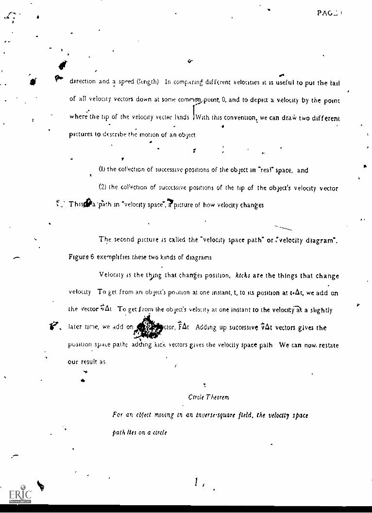
I041. direction and a sped (itngth) In comparing different velocities it is useful to put the tail

of all velocity vectors down at some comrncrp,ipoinr, 0, and to depict a velocity by the point

where the tip of the velocity vecter lands JWith this convention, we can draCv two different

pictures to describe the motion of an object

01 the collection of successive positions of the object in "rear space, and

(2) the collection of successive positions of the tip of the object's velocity vector

ThisigraIAth in "velocity space",lpicture of how velocity changes

The second picture is called the "velocity space path" or :velocity diagram..

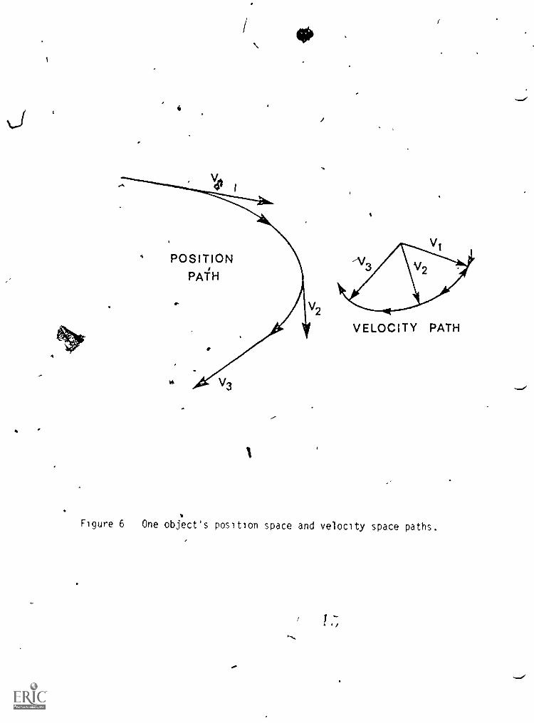
Figure 6 exemplifies these two kinds of diagrams

Velocity is the thing that changes position, kicks are the things that change

velocity To get from an object's pn,ition at one instant, t, to its position at tsAt, we add on

the vector :Ivtit To get from the object's velocity at one instant to the velocity at a slightly

later time, we add on ctor, FAt Adding up successive At vectors gives the

position space path: adding kick vectors gives the velocity space path We can now restate

our result as

4

Circle Theorem

For an cbleci moving to an inversesquare field, rAe velocity space

path lies on a circle

It

U

/

POSITION

PATH

II.

,

0

1

I

I

VELOCITY PATH

Figure 6 One object's position space and velocity space paths.,

4

-..

PAGE II

To avoid confusion we point out that the center of this circle is not necessarily at

the.origin in velocity spay:* "N

1,,

4 The Velocity Space Path. ,

. -

Our Circle Theoren tells us that the velocief space path lies on a circle But is iti- a complete circle or just part of it? We can answer that qtiestion and a bit more

M.

1

We showed that an orbit which does manage to get all the way around the sun

crosses every half -line from the sun exactly once Such an orbit is a simple closed curve

In a complete levolution,tbererote, the direction of the planet's velocity vector must change

through 3600 (See referl'nce 4) That means that in velocity space Ikokthe path meets every

half-line from the velocity, space origin it follows that closed orbits in position space

correspond to complete circles in velocity space, and we have learned, besides, that the

origin of velocity space i's u4de the circle

,

We now have a good qualitative picture of the velocity space path for a closed

orbit (Open orbits are discussed in section II) In Fait II, we will extract information about

the position space orbit from our velocity space diagram

IL invariant5 of the Orbit

5 Angular Momentum

PAGE 12!

As we have seen,Ihe velocity space path of a planet in an inverse-square field lies

on a circle One obvious Invariant of a circle is its radius How can we interpret this

invariant physically?

We got the circle in section 3 as the result of the algorithm "forward distance D,

turn angle A8, repeat" As one can see (Figure 7), this generates a circle of radius DIGS In

dgirour case Ae was an arbitrary small angle and D was the magnitude of the kick Ftit over

the corresponding small piece of orbit. Le Lung u denote the radius c the velocity circle, we

have

tu

It is not immediately obvious that this is a constant However, we can simplify the

expression using the fact from geometry that the area swept out over a small piece or orbit

IS

A - r2M2

Then u-ZAL- Fr2trt We can eliminate Ole apparent dependence on the non-constant termAe

r2 by using F-K/r2, we obtain

u(2/Xt

.../....

.

,01...w,

I

r

D

Figure 7 D= radius x 6 0

t

f

PAGE 13

The 'term 2Aftit, which tells how fast the planet IS sweepinga.out area, is precisely the

cbnstant called angular momentum, L (See Appendix ) Therefore

The radius of the velocity circle equals the force constant

K divided by the angular momentum L uKa..

For a fixed gravitational field, the radius of the velocity circle tells us the planet's angular

momentum a larger radius gives a smaller angular momentum.

1

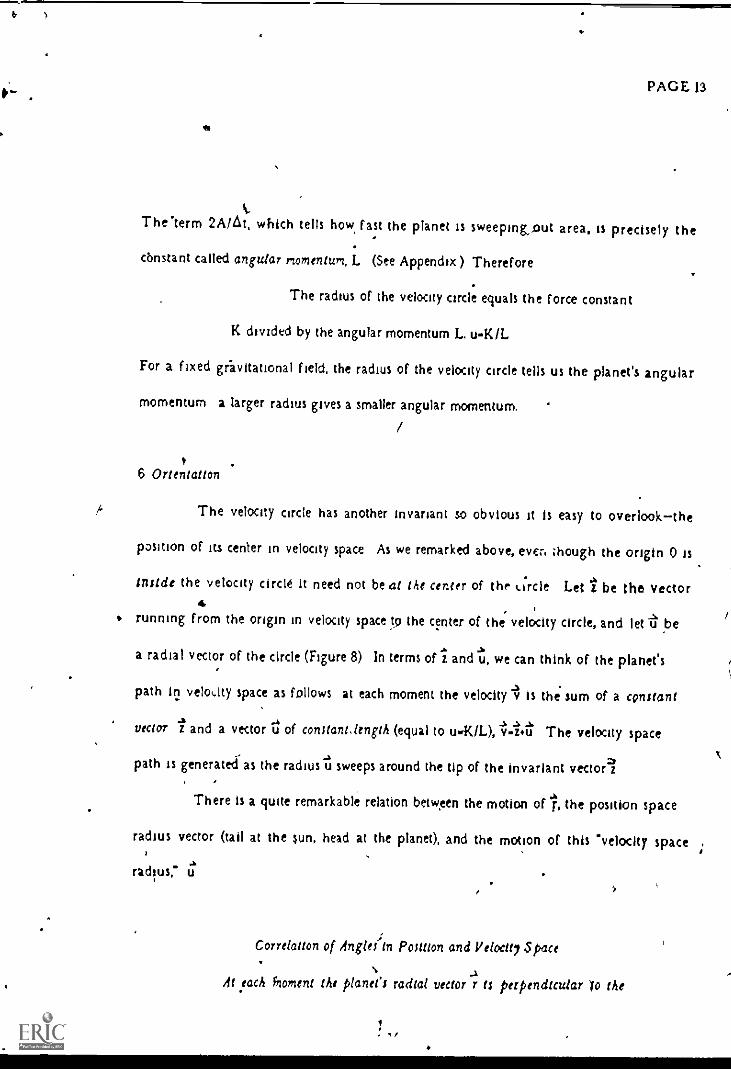
6 Ortentatton

The velocity circle has another Invariant so obvious it is easy to overlookthe

position of its center in velocity space As we remarked above, ever, though the origin 0 Is

Inside the velocity circle It need not be at the center of the circle Let t be the vector4

running from the origin in velocity space to the center of the velocity circle, and let 11 be

a radial vector of the circle (Figure 8) In terms of i and -bu, we can think of the planet's

path In velot.Ity space as follows at each moment the velocity 'v is the sum of a constant

vector i and a vector t of constant length (equal to u-KIL), -Mt The velocity space

path is generated as the radius u sweeps around the tip of the invariant vector i

There Is a quite remarkable relation between the motion of T, the position space

radius vector (tad at the sun, head at the planet), and the motion of this -velocity space

radius; it

Correlation of Anglelin Position and Peale, Space

At each fnoment the planet's radial vector r es perpendicular to the

ORIGINsINVELOCITY

SPACEI

C

Figure 8: The invariant I.

CENTER

OF CIRCLE

radius u of the velocity circle

,

PAGE 14

To see this we examine how the kicks fit into both diagrams In position space each kick is

Parallel to the radial vector r In velocity space the same kick is tangent to the velocity

circle and hence perpendicular to the velocity circle radius u.

Hence'u is perpendicular to r

Correlation of Angles is a powerful principle It tells us

(I) Each point on the velocity space path corresponds to a unique point in the

planet's orbit (The planet cannot attain the same velocity at two different points in Its

orbit)

(2) The planet's position vector sweeps around the sun at the same rate and with

the same direction (clockwise or counter- clockwise) as its velocity sweeps around the circle

in velocity space The two are always SO degrees out of phase (Figure 9)

. I Now we'can,give more meaning to the a vector The planet's speed, v, is

' greatest when the u and z vectors are lined up, least when they are opposed v min.u:z,tr'

v ma xIsitz Therefore the z vector points in the direction of maximum speed and

opposite to the direction of minimum speed

The points of greatest and least speed occur where the velocity vector is parallel

.-.)

to u,afid so perpendicular to the position spar ,e radius r It is not hard to show then

that the point where speed attains its maximum (respectively, its minimum) corresponds to

the minimum (respectively, maximum) distance from the sun The reader can fill in the

details of the proof sketched below

r

POSITION

-I-

VELOCITY

POSITION

-3-

VELOCITY

VELOCITY

Figure 9 Snapshots of position and velocity over an orbit tri_1^6.

PAGE 15

Step 1 At a maximum or minimum distance the velocity v must be

perpendicular to the radius r

can occur

Step 2 The velocity diagram shows that. there are precisely two points where this

Step/3 Conservation of Angulaik Momentum implies that rmax corresponds to

v min and rmm to vmax

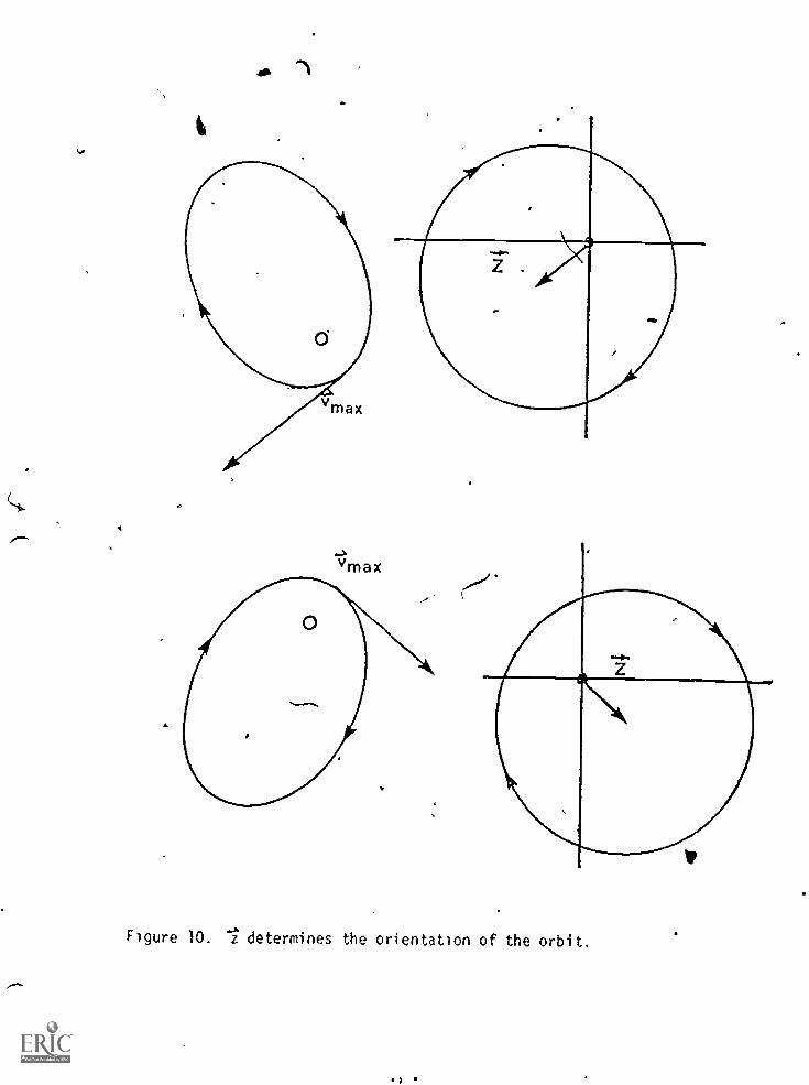
Now we have some more qualitative information about the shape of the orbit

there is precisely one point of maximum distance from the sun, and one of minimum

distance They occur on opposite sides of the sun since the corresponding u_s

vectors point

in opposite directions The z veCtor determines the orientation of the orbit. It points inAI%

the direction of maximum speed (Figure 10)

7 Shape and Symmetry

What more does the length of -2 tell us about the orbit? Consider what would

happen if t vanished There would then be no direction picked out for maximum speed

or distance from the sun The planet would have to travel around the sun in a circle at

uniform speed (Another way to see this ti would be equal to -6" and therefore always

perpendiciular tot and of constant length -the characteristic of uniform circular motion )

This suggests that z indicates how the orbit deviates from a circle. We can

make this precise One obvious measure of the non-circularity of the orbit is the difference

In the extreme distances-from the sun,

c

t

._.1

vmax

Figure 10_ 1 determines the orientation of the orbit.

) '

L

rmax rmin

PAGE 16

If we want an invariant that depends only on the shape and not the size of the orbit it is

better to see how much the ratio

rmax rmin

differs from 1 The length of z, relates the maximum and minimum speeds

vmin.u-z .tiozvmax

To relate speed to distance from the sun we use angular momentum. If the angular

momentum is L then

vmin x rmax vmax x rmin

because at these places in tie orbit v is perpendicular to r (Section 6) Therefore.

rmax Vmax

rmin Vmin

Since u -K /L we can also write

rmax

rmin

Kt LzK- Lz

U + Z

u z

But K depends only on the nature of the gravitational field so we see that our "shape

invariant" is determined by Li The larger Lz, the more the orbit deviates from a circle

In section 11 we will derive the analytic result that the orbit Is an ellipse and Li determines

its ectentrtctty

In fak< knowledge of K and the velocity diagram essentially determines the

planet's motion The maximum velocity can be read off the diagram Immediately, as can

u.K/L, so we know L The shortest radius in position space has length rmin-Liv and

r

PAGE 17

is perpendicular to vma\k (Section 6) Having this one vector,imm, we can generate the

orbit starting at the positiOn determined by timo with the following algorithm

I Travel a short distance,:qn in the direction of v

2 Measure the change in angle, M, in position space.

3 Find the velocity ar this new angle (by rotating u through GB and consulting

the velocity diagram)

4 Return to step I This generates the entire position space path

Notice that the velocity diagram is symmetric about the line determined by z.

The above algorithm translates this fact into a symmetry of the position space orbit

Starting at the nearest point to the sun, construct the orbit in the forward direction for a

while, along vi for COI, then along st for A02, and so on Now go back to the

starting point and run the algorithm backards with the same sequence of GB's Since the

velocity diagram Is symmetric we generate the same small segments of orbit, except that they

have been, flipped about the line perpend \cular to i Therefore the entire orbit is

symmetric abouit this line

8 Summary

We have so far obtained the following irkormation from the velocity diagram,

The wdius of the velocity circle dete\mlnes the orbit's angular momentum.

uK/L

2 The center of the velocity circle determi es the orientation of the orbit (t

.),

4it

1

i

:.

it

4.

1

,

s

PAGE 18

. . A

0

points in the direction of maximum speed) and its 'shape" (Li determines rmax/rmin).Q CP -...

3. From the velocity diagram, we can algorithmically determine the whole orbit.--

vs

-J

o

44,

,----"---

174

I

1

S

i a .

1 4k

Sr

.7r

e

46

\/

i

i

.

..0......

I

o.,=...

r

i

PAGE 19

M. Perturbations * \

9 The Perturbation Formula, Radial Thrust

4it is in the study of perturbations, or how orbits change under small kicks other

than those given by the sun, that our use of velocity diagrams really pays off. It pays off

for a very good reason, which we mentioned in the introduction as a qualitative form ofI

Newton's Second Law of Motion 4

(^, Force acts on the paths of particles by changing velocity and not

position

If we fall to take account of this fact we may be faced with sltuation3 that appear

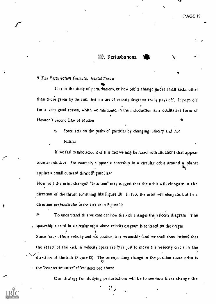
counter intuitive For example, suppose a spaceship in a circular orbit around a planetIS

applies a small outward thrust (Figure 11a)-

How will the orbit change? "Intuition" may suggest that the orbit will elongate in the

direction of the thrust,, something like Figure lib In fact, the orbit will elongate, but in a

direction perpendicular to the kick as in Figure lic

A To .understand this we consider how the kick changes the velocity diagram The

spaceship started in a circular at It whose velocity diagram is centered on the originI

Since force affects velocity and not position, it is reasonable (and we shall show below) that

the effect of the kick in velocity space really is just to move the v-elocity circle in the

direction of the kick (Figure 12) The corresponding change in the position space orbit is

the "counter-intuitive" effect described above

Our strategy forstudying perturbations will be to see -how kicks change the

,

1'

1

...

...

A

N

.

..r

)

C

Figure 11 Will the outward kick on orbit (a) produce 0) or (c)7

4 i

MO

4

r

POSITION BEFORE

t`

POSITION AFTER

VELOCITY 43EFORE../-*".-....

I

VELOCITY AFTER

Figure 12 The perturbation induced by an outward kick.

PAGE 20

velocity diagram More precisely, we know that the shape and orientation of the orbit is

determined by Lt, the i vector times the angular momentum, so we want to find the change

in Li, A(Li), produced by an arbitrary kick

The basic velocity space equation, 7," I u, gives Li L-4 Luu Since tti has

length KIL we have Kt, where i Is a vector of unit length whose direction is

determined solely by the object's position (It is perpendiculaito the radial vector t) To

compute the effect of a kick tt-v.1 on Li - Lv Kt notice that since kicks do not affect

position,1 is unchanged K is also unchanged Therefore the changein Li Is the same as

the change in Lt, and the first-order approximation to the change in a product of

changing quantities gives ,,,

Perturbation Formula A(Li) -la LA-st

We can use the Perturbation Formula to tidy up our discussion of the "radial

thrust problem",(Figure H) Since Ast Is in the radial direction, the angular momentum

does not change (AL - 0), so the formula implies A(Li) . LASS. This means that the

velocity diagram changes from a ai vector of zero to a"i vector in the direction of Al

(Figure 12)

Intuitively, the velocity circle is "pushed" in the direction of the kick Note that an inward

kick at the bottom of the position space orbit would have the same effect

/

4'

POSITION BEFORE POSITION AFTER

VELOCITY BEFORE VELOCITY AFTER

/

Figure 13: The perturbation induced by a tangential kick.

,..

PAGE 21

V

10 Thngenttal Thrust, Solar Wtnd, r.(244) Lawsa

4

In this section weapply the Perturbation Formula to some other orbit problems

ITangenttal Thrust Suppose again that a rocket starts in a circular orbit, but this

(. time provides a tangential kick (Figure 13) To determine A(Li) a IML LAI we note that

-1 \vilL is an impulse in the direction of AI since AL Is positive and I is parallel to AI..,

Then the newly created z vector must be in the direction of the impulse (Figure 13) The

elongation in position space is again perpendicular to the kick

The S'olar Went:15 Assume the. rocket is affected not only by the planet's gravity

but also by a small constant force (Luehrmann's 'solar wind') If the perturbing force is

small compared to gravity, each revolution of the rocket will be nearly an ellipse. We can

therefore think of the orbit as an ellipse latch vanes througr time To compute how the

ellipse changes we view the wind as providing impulses all along the orbit (Figure H) and

sum A(d) - liAL LA,t over one revolution

, The LAI contribution Is a net change in the direction of Li-sit To compute tAL

we notice that AL Is positive on the bottom half of the orbit and negative on the top half

as shovtri in Figure 15b We can sum the t AL's by exploiting the symmetry of the orbit

The vertical components of thersliAL's on the left cancel the vertical components of the

,vALs on the right, leaving only a horizontal component In the direction of At (Figure

15c) This adds with LAI to produce a i" vector In the direction of the wind Intuitively,

the velocity circle gets 'blown' In the direction of the wind The orbit elongates

perpendicular to the wind as in Figure 16

1

I

.1

4

Qv

Figure 14 The solar wind.1.__

t

../

)

...

)

I'

.p...911.

--..,WIND ...

A

C

4`

B

/

-\,-A L

f

,Figure 13. The vectors I (a) and -v1AL (b) for the solar wind. .In (c)

we see that the vertical components of I'IAL on the left

cancel the vertical components on the right

R 1 1

,.,

p

Figbre 16. Position space charge in the orbit under the solar wind.

7i

)

PAGE 22

4

Since the wind does not affect the symmetry of the orbit about the vertical axis we can

apply the same analysis as above to show that the Li vector continues increasing In the

direction of the wind From this we conclude that the orbit becomes more and more

eccentric while the direction of i remains constant, and the orbit continues to elongate

perpendtcular to the wind

The orbit becomes closer and closer to a straight line, and it eventually reaches a

point where the "small" wind can hay rge qualitative effects over a timescale of less than

one revolution (the orbit In fact reverses direction), and our method of averaging over an

entire revolution becomes inappropriate

The 1(24) Force ,eld If e is a small constant (we will take it to be positive), we

can treat the central force field of magnitude ((Z.() as a perturbation of the (2 field The

perturbing force is some force (positive or negative) In the radial direction To understand

how this perturbation affects the orbit, we make the important observation that the shape

of a r -2 or r-(24) orbit noes not depend on the scale which we use to measure radius

Therefore we can determine shape by using any scale which makes it convenient to

compute the effect of the pfiturbaliun 1-ui the orbit shown in Figure 17, we scale to make

the distance OP equal to one Since 1/r2 < 1/r(241) for r < I and 1 /r2 > 1/r(2') for r > I the

perturbing force is as shown

For this perturbation the kicks are radial, so L is constant This means a(Li) -

LAr, but from the perturbation formula, AL = 0 implies A(Li) = LAI? Hence At- A?

Now we can sum -AZ over an entire orbit The left-right symmetry of the orbit and

perturbing force means that the sum of horizontal components of the kicks must cancel,

:3

(

%

-Figure 17: Orbit with perturbing force indicated 'for r-(2+0

.

`3J

,

L\I"

,-

1

/Figure 18 A z perpendicular to e_

....,...,

f

t

--,

er

AO .

Figure 19: Precession of r-(2+E)

orbit.,

I i

/

N

0

(4

I

..e

4

.

e

a

(

it ,

/ 0

i

V' Atm t. Zi.i

cg,

W ---,

and the isC'z' is downward, that is, perpendicular to the original i Subsequessittlis will be....1,..,

...aperpendsisolar to the current z and this results piimarily in a rotation of z, not a change in. ./... length (Figure 18) The "major axis" of the position space orbit, by the consequences we

' Ne

derived f ronlior relation of Angle; must follow this counter-clockwise otation Though

the orbit retars its shape Li, it precesses (Figure 19) .J. 4

ii, Warning It should be remarked that in't/he preceding two examples we looked at....--,.

the f. vectors as representing A"v1 for the perturbation formula Of course we should haveP

used 'Fat, but, because ill the symmetry involved, the At factor can be ignored in those twx, ....,,....,.

cases In more complicated situations, though, this does become an issue For example, we

f,

1 /

invite the reader to use the techniques of this sck.tion to tieat the F. rturbation induced by...

. -..an oblatessun

i

II The Orbit is a Conic Section

a

IV. Finblytic Results

Ir. k

I

I.

..

I

An objection that is sure to occur to some of our readers goes something like this.A

4 et"All these intuitive methods are fine, bait if you want useful quantitative information you

have to return to the standard differential equations you've been trying to get along'CI

without" . t..

.,

I

1 a

,..

e 4.

.4

rr.....,

r.

.....'"-

1

*41

I

PAGE 24

Of course there are orbit problems our simple methods won't handle As for the

standard results, however, we are able to derive the orbital equation directly from our

velocity diagram/using no more than trigonometry.

do

4.

The orbit is describes in polar coordinates by the equation

Lr ru - z cos9

The proof is a natural correlation of the basic quantities, t,ta, d, I and L using4

._.;"the definition of angular momentum At a point in the orbit when the t vector and the z

vector differ in direction by an angle 8 we construct the angular momentum triangle (see

appendix)

<-7

The area of the triangle OAB in Figure 20 is 4 definition L12 If h is the height

1 1

of the triangle itn

L_ r h2 2

.,

a.

Since u and r are perpendicular, the height of the triangle is given by h - u z cos 8.

Therefore

aft

L - rh - r (u - z cos e)

Here e represents the angle in veloctPripace between i and the fixed vector 2 Correlation

--of Angles implies that e also measures the angle in position space from to a fined lector

$

lb.

.1

.6.

N

4

F)gure 20: The angular moment.w, tn)ansle W.'40

S

440

mMi MEW mu...M. .11. MEM m

I

'1 . 1 A

I'

z cos°

0,

r

POSITION

# .r

,

11.

N. \ .,,

POSITION1

i

VELOCITY

POSITION--'0

r VELOCITY

Figure. 21' Sample id-bits in position and velocity space.Y

+1

..

1t

4

/..j

...

PAGE 25

perpendicular tot Therefore r and 0 are polar coordinates in position space

The above equation describes a conic section When the origin of velocity space

lies within the circle, u>z and the orbit is an ellipse When the origin is outside the circle, u

< z and the orbit is hyperbolic When th.e circle passes t6rough the origin, u - z and thet

orbit is parabolic (Figure 21)

Writing the equation to the farm

yu,r -1 (z/ )cos0

2L //K

I -00 cos 0

Lz/we get the "standard forrn" for a conic section and see that / K is the eccentricity, and

r r2 rir... r r-N. is the radius of tile orbit when the eccectricity is zero

Ye

12 Conservattoh of E Ttfr gy

Energy conservation does not apse naturally using this geometric approach

although we can obtain the result as a simple application

Apply the law of cosines to th velocity diagram in Figure 22 to get

MP

i.

,

,./

'

Figure 22: v2 z2 + u2 - 2uz cos0.

a

4.

PAGE`26

2 2 2-r 2uz cOse

sum. z core 1.1 - (from Section II) we obtain

2 2 2 2 u Lz

and hence (since u

2K

r

72

Z2

U

2 r 22

z2

u

Since z and u are constant for the orbit, 2 is a constant, total energy. E It is

interesting to note that when the Wanet crosses the semi-rnino' axis ('perpendicular toV) V.vz

T. and -; form a right triangle with v2.u2-13, hence the kinetic energy /2

negative of the total energy there

13 Kepler's Third Law

is exactly the

We can use the relation of angular momentum to area swept out, 2A-Lt. to

compute the period of the planet's` revolution In one period the planet sweeps out the

entire area of its elliptical orbit The area of an ellipse of semi-major axis a and

eccentricity e is given by A - T a\17-7; For the orbit we have

a

1

2

The eccentricity is e - ziti, so

(

Then the Period is determined by

Or

rmin + max

L T = 2 - a2 j 1 e2

T2- a 3 /2 \a

L u

Mr....1=.1.

=

rL

2 U - z

LU

U2- 2

r., 52- Z2 .1: in----

+

U U 5--

2 ra1/2 ITT

u 17

2 7 '/2''FIT -

In terms of quantvies appearing in the velocty diagram we gett.-

14 Op-en Orbus

following

27.;(u2 - z 2 ) h

... 2 rk' '2E)3,

PAGE 27

U I z

K2 2U - Z

fa

t.

Rather than treat the hyperbolic case in detail, we leave the reader to verify the

1 For an open orbit, the arc of the velocity circle which is actually traversed is the

part shown below, bounded by the tangents to the circle through the origin of velocity

spice Velocity space geometry gives the correlation of energy with limiting velocity. v

/i

....,"

)4,

,/

r

i

I

Figure 23 The velocity ch agra-n fcr- an open orbIl t

47

(

?

......."

v.,'

,,

Figure 24. Deflection angle for an open orbit.

M

t

I,

r

r ro-p t. 40

-.FRP r.1T(Figure 23)

2 The deflection angle (angle between the two asymptote: of the hyperbola) can

6be,easily found as a function of energy and angular momentum tan '1.2E---- (Figure

2K

24)

15 Suggest:ow for Further Research

We have by no means exhausted the study of the geometry of orbits In this

paper The geometry of orbits, particularly the perturbation theory, is a rich source of

problems, even of mini-research projects of the type described by Luehrrnann5. Below we

make some suggestions for problems and study topics

An inSlrucittit paradox The Galilean transformation requires the relation between velocities

measured in two different frames of refrence moving with relative velocity vo to be vIF .--1.- v

_.s.

v_).

o This it is a simple matter to rno.ie into a frame with relative velocity -z and transform(

the za

vector for an elliptical orbit to 0 Why then does one not observe a circular orbit In

the new frame? In particular, what fails in the algoi ithm of Section 8 which does generate

a circle in position space given a circle centered about the origin in velocity space?

An Aid to Aitrogation? Suppose we had to pilot a spaceship in a gravitational field (such as

simulated in computer "space war" games) Would a velocity diagram be a useful addition

to our instrument panel? Poi example, to change from an elliptical Alt to a circular orbit

5 1

6 "

. PAGE 2

.-we need only corrsult the velocity diagram and apply a force to cancel the z vector, On the

other hand, lots of information is lacking if we use only the velocity picture Intercepting

another spaceship is a tricky problem involving timing (Although merely matching its

orbit is easy ) What other instruments should supplement or possibly replace a velocity

diagram?

Geometry of the harmonic. oscillator A i undamental geometric property of solutions to the

_1/1-2 differential equation is that they have a vector constant of motion (tor the maximum

ivelocity, or the Runge-Lenz vector are all possible choices for this constant) The two

dimensional harmonic oscillator with equal mode frequencies has a similar structure.

Solutions have an obvious axis which may also be assigned a magnitude in any number of

ways Can one develop a useful velocity space geometry for that system? Can one treat

simple perturbations, as with orbits? ../

'v.

More Solar Wind A further discussion of the solar wind phenomenon could make use of

the fact that the force field is conservative and therefore the energy of the orbit is constant

This implies that the angular momentum decreases as the orbit becomes more eccentric..

Thus the velocity circle is not only *blown by the wind" but also the radius becomes larger( .

and finally infinite when the orbit degenerates to a line, Show that thc changing velocity

circle always passes through two fixed points in the plane (Figure 25) .

Our method of averaging over entire orbits is only a first-order perturbation

theory whereas the formula

d(L,I)I.

d C'+

ds dsd1..

ds

v

-a

at

...

,

.."."'".

,-....-..

JI

Figure 25: Changing velocity circle under solar wind.

i . 0

4

PAGE 30

a

(s is any parameter) is exact One would like to have a treatment of the solar wind which

, works near the turnaround points, au approaching I

Finally, is there a complete perturbation theory based on the geometry of orbits?

In particular how can one treat perturbations out of the plane of the orbit?

I.

ge.

A I

appendix:Angular Momentum and Kepler's Second Lawa"i

PAGE 31

leThroughout this paper we have been assuming Kepler's Second Law There is a

-Nif simple geometric proof of this which we place here in an appendix because tt did not

originate with us It can be found in Newton's Principle'

a

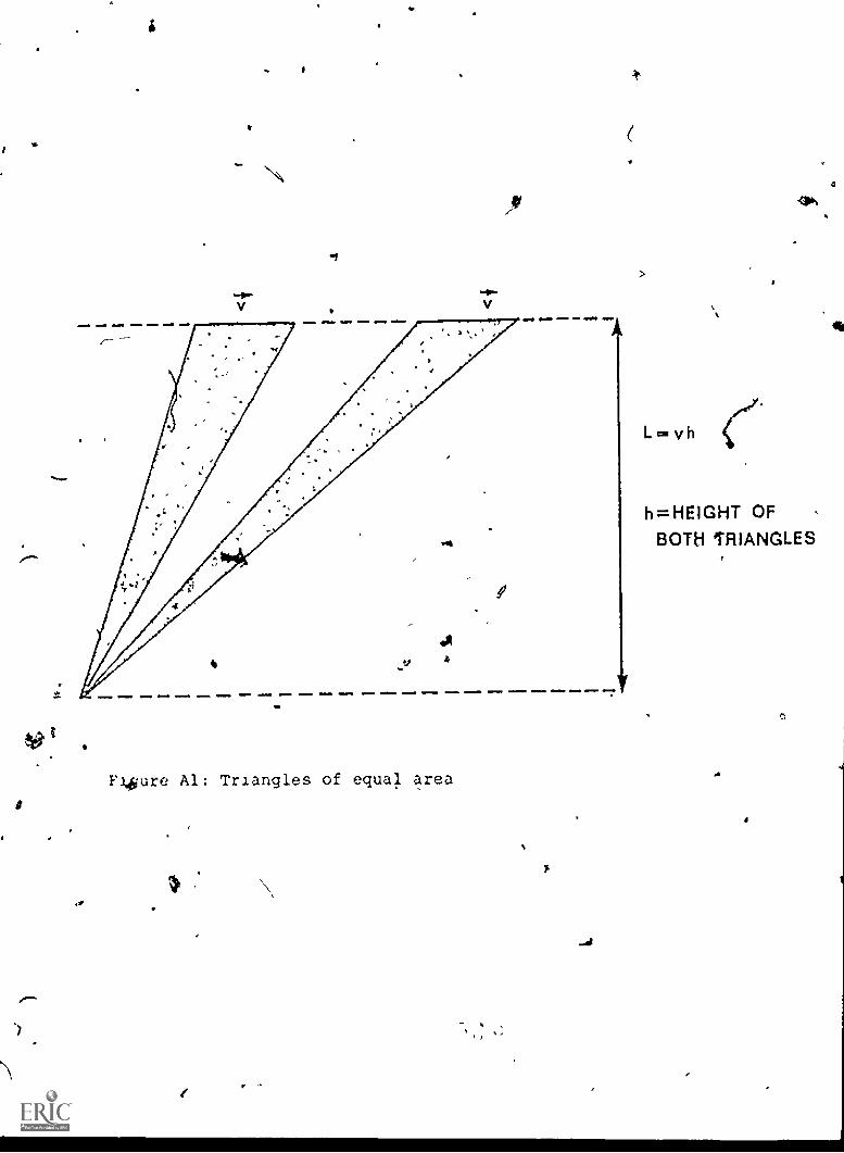
The angular momentum, which wesclenote by L, is defined to be twice the area of

the mangle determined bythe velocity vector and the radius vector from the sun to the

planet As shown below L Is constant if the velocity doesn't change the triangles have

equal areas since they nave equal bases (the length of $) and equal height* (Pipit* Al),- .

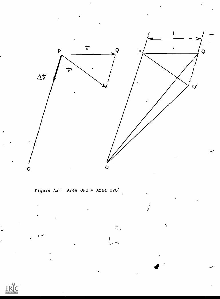
More remarkably:et remains constant if we change the velocity by applying any kick in the

radial directton (towards or away from Chem in) The effect of a kick XV' on the angular

momentum triangle is illustrated beloai (Figure A2) The kick changes v to v but triangles

OPQand OPQI have the same base, OP, and the same height (h in the diagranksince OP

6and QQI, aie parallel Therefore OPQ and OPQf have the same area, and angular

momentum is unchanged

A planet moving about the sun, subirct to no force but the sun's gravitation, has

every kick applied in the radial direction None of These change the angular momentum,

, is therefore an Inver iant or the planet's whit To find a geometric interpretation of

this fact, OF cotamine the orbit at time intervals At small enough that the velocity does not

chan4ge much over each interval In each interval the radius vector sweeps out a small

triangle . The area of one of these small triangles is

CZ'

'WM

V

N\

6

V

96/t

tif

_1r

11.* - --

F4eure Al: Triangles of equal area

,,

1

>

L'vh

Ob.

h=HEIGHT OFBOTH TRIANGLES

04

0

Figure A2: Area O?Q = Area OPQ'

.

t

4

I

1

44

F

Mir

43 / -P,AGE 32e*

4.

I,1(base) x (height) . 1 / I

1.-,It xt)= t2 2 2

1(h as i figure Al) The total area swept out over some long time

T .6ti « At2 «

is the sum of the areas of the small triangles

t I

A= La t1 +2 L a t2 -p21 qa ti+ At 2-r- )21-- L T2

ti

)

..k

\.

This gives Kepler's Second Law

For a body moving in a radial force field, the radial vector switiv

out equal areas in equal urns},

S.

It is unfortunate that this proof is not more often presented in ph4sics courses (although

Feynman 6 discusses it and there is a movie7 demonstrating this argument)

d

In

/1

y,e

y

i PAGE 33

Rotes and References

I S Papert, 'Uses of Technology to Enhance Education'i

Al Memo 298, MIT Artificial

Intelligence Laboratory, Cambridge. Mass. 1973

2 We consistently set m - I, as the mass parameter Is quite irrelevant to these orbital

discussions

3 This fact is one of the first theorems in Papert's Turtle Geometry In that context it is

an empirical theorem routinely used by children in directing a computer- controlled "turtle"

to draw circles See S Papert, 'Teaching Children to be Mathematicians vs Teaching

Them about Mathematics", Int J Math Educ Sct Technol , V oi 3, 249-262,1972

4. This Is another theorem in Turtle Geometry It Is called the Total Turtle Trip Theorem,

and states, if a WI tie moves around a simple closed curve Its heading changes by precisely

360 Here, the heading corresponds to the direction of the velocity See Reference I

5 This pheoomenon was introduced to us by Arthur Luehrmann whose article "Orbits in

the Solar Wind", Ant J of PAys,, Vol 42/5. May 1974, Indicates many areas of research

dealing with the solar wind

6 R P Feynman, lip Character of Physical Law. Cambridge. MIT Press, 1965

7 B Cornwall, C Cornwall, and AM Bork, Newton's Equal Areas, International Film

Bureau, Chicago, 1957

I,!I .: - n'4-

No.