Embed Size (px)
Citation preview

BUDI NURANI RUCHJANA
DEPARTMENT OF MATHEMATICS
FACULTY OF MATHEMATICS AND NATURAL SCIENCES
UNIVERSITAS PADJADJARAN
Indonesia
Paper is presented at SEAMS School
Spatio Temporal Data Mining and Optmization Modeling
UTC-Bandung, 9-19 August 2016

Development of Sciences and its Applications using a natural resources and environmental for welfare of society
Cooperation Institutional Supporting Publication Application
Mathematics Chemistry Physics Biology Statistics
National
International
Material and equipment
Supporting financial
Journal
Book
Scientific meeting
PatentI
Technology and science
Society
Pure Math
Applied Math
Computer Sciences
Organic Che
Natural product
Biokimia
Anorganic Che
Physical Che
Analitical Che
Instrumentation and
Processing Material
Dvanced Material for
renewable Energy
Kehandalan Pembangkit
Daya & EBT
Applied Geophysics
Conservation bio
Mikrobiology
Human ecology
Ecotechnology
Social Stat
Bussiness Stat
Industrial Stat
Biomedical Stat
Funtion Bio
Bioassay &
Environment monev
Research Roadmap of Faculty of Math and Natural Sciences
Universitas Padjadjaran
PIPUNPAD
Research on Basic Sciences
Model SAR, SAR-Kriging, Cross
Variogram, Co-Kriging
Model Clustering GSTAR, GSTARI-SUR,
GSTARIMAXDisease mapping
Model Clustering GSTAR-Kriging menggunakan
KDD
Pengembangan Model
Spasial
Pengembangan Model
Spatio Temporal
Pengembangan Model Spatio
Temporal Data Mining
Industri, Pemda, Himpro, PT DN-LN
Prototype AplikasiModel Space Time
Jurnal internasional, Hak Merk
Kerja samaAplikasi Teknologi
InformasiPublikasi, HKI
Metodologi KDD
Multivariat geostatistika
dalam prediksi panas bumi
Kestabilan lereng
Open source R, Matlab
Excel VB
Aplikasi user friendly
Hak Merk Model Clustering
GSTAR-Kriging
Statistica Neerlandica,
Journal Data Mining, SOLA
IJAMAS, JIMS
ITS, IPB, RuG, LEAD
Leiden, IndoMS
LAPAN Bandung
Pusair, Balai Pangan
PERTAMINA
PIP Unpad
CG Jabar
Multivariat time series
untuk bidang keuangan,
pendidikan dan lingkungan
Metode penaksiran:
SUR, Bayesian
Algoritma integrasi clustering
spatio temporal dan
SDM ethnomathematics


2010 Mathematics Subject Classification :62M10 (TIME SERIES0, 63M30 (SPATIAL PROCESSES), 62H11 (SPATIAL STATISTICS)

A STOCHASTIC PROCESSES IS A FAMILY OF RANDOM VARIABLES X(t) PARAMETRIZED BY
WHERE . (OSAKI, 1980)
WHEN {T=1, 2, 3, ...}, WE SAY X(t) is a STOCHASTIC PROCESS IN DISCRETE TIME
WHEN T IS AN INTERVAL IN R (TYPICALLY
, WE SAY X(t) is a STOCHASTIC PROCESS IN CONTIONOUS TIME
Tt RT
),0[ T

Random Variable a realization of
TttX ),(
)( 1tX
Set of all realizations of
is a state space of S
( )X t
S discrete S continous
Proces is called a chain
Proces
T
Parameter Indexes
T discrete
T continous
Stochastic Processes
)( 1tX
Stoc. Pro. in discrete time
Stoc. Pro. in continous time

THE AIMS
•To develop study on a space time models, especially on the Space Time Autoregressive (STAR) and Gene-ralized (GSTAR) model.
•To inform the research activities on application of the space time models.

TO INTRODUCE THE SPACE TIME MODELS BASEDON TIME SERIES MODELS FROM BOX-JENKINS (1976AS PART OF MULTIVARIATE TIME SERIES ANALYSIS)
TO EXPLAIN THE SPACE TIME MODELS, FOCUS ONTHE STAR AND GSTAR MODELS
TO EXTEND THE GSTAR-ARCH, GSTAR-SUR ANDGSTAR-KRIGING MODELS
TO APPLY THE STAR, GSTAR AND GSTAR-KRIGINGMODELS TO REAL PHENOMENA SUCH AS OILPRODUCTION DATA AT VOLCANIC LAYER INJATIBARANG, CLIMATE PHENOMENA IN INDONESIA

FURTHER RESEARCH : CLUSTERING SPATIAL OF GSTAR-KRIGING
GSTARIMA-X MODEL
DEVELOPMENT STUDY ON THE SPACE TIME MODELS
GSTAR-ARCHGSTAR-SUR
CLUSTERING GSTAR-KRIGINGGSTARIMA-X
GSTAR-OLSSTAR
VAR M-ARCH
AR, MA, ARMA, ARIMA
ARCH, GARCH,ARMA-ARCH
TIME SERIES MODEL
HOMOSCEDASTICITY HETEROSCEDASTICITY:
WEIGHT MATRICES W


3
DATA
IDENTIFICATION
ESTIMATION
PARAMETER MODEL
CHECKING DIAGNOSTIC
Box-Jenkins’s Procedure in Analysis of Time Series
-MODEL
-PREDICTION
Space-Time Model
Checking on stationary
Identification Process
Checking diagnostic
Fitted Space-Time model
Prediction
Y Y
Y
YN
N
N N
12
Parameters Estimation
The random weight matrix W
Fitting theoretical model
to experimental semivariogram
Semivariogram Estimation
Characterization of weights(independent of time)
Parameters estimation
and checking diagnostic
Identification process
Study on Stationary
Univariate data from each location
Space-Time Phenomenon
Procedure in Space-Time Analysis
Source: Box-Jenkins, p. 19
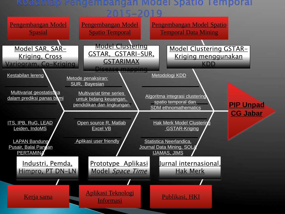
time Bandung (Kota) Bandung Bandung Barat Banjar (Kota) Bekasi Bekasi (Kota) Bogor Bogor (Kota)
Jan-81 25.2 23.8 25.2 26.3 27.0 27.0 27.0 27.0
Feb-81 24.9 23.5 25.0 26.0 26.9 26.9 26.9 26.9
Mar-81 25.5 23.8 25.6 26.5 27.3 27.4 27.4 27.4
Apr-81 26.1 24.5 26.2 27.2 28.1 28.0 28.0 28.0
May-81 26.3 24.6 26.4 27.2 28.2 28.3 28.3 28.3
Jun-81 25.4 23.6 25.5 26.2 27.4 27.4 27.4 27.4
Jul-81 25.1 23.4 25.2 26.0 27.0 27.1 27.1 27.1
Aug-81 26.1 24.3 26.2 27.0 28.0 28.0 28.0 28.0
Sep-81 25.8 24.2 25.9 26.8 27.8 27.8 27.8 27.8
Oct-81 26.5 24.8 26.5 27.4 28.4 28.5 28.5 28.5
Nov-81 25.3 23.6 25.4 26.1 27.3 27.4 27.4 27.4
Dec-81 25.2 23.7 25.3 26.2 27.1 27.2 27.2 27.2
Jan-82 25.0 23.6 25.1 26.1 26.8 26.8 26.8 26.8
Feb-82 25.3 23.8 25.4 26.4 27.2 27.2 27.2 27.2
Mar-82 25.5 23.9 25.6 26.5 27.4 27.4 27.4 27.4
Apr-82 26.1 24.5 26.2 27.2 28.1 28.0 28.0 28.0
May-82 26.0 24.3 26.1 27.0 27.9 28.0 28.0 28.0
Jun-82 25.2 23.4 25.3 26.0 27.2 27.2 27.2 27.2
Jul-82 25.7 24.0 25.8 26.6 27.6 27.7 27.7 27.7
Aug-82 25.8 24.0 25.9 26.8 27.7 27.7 27.7 27.7
Sep-82 25.5 23.8 25.6 26.5 27.5 27.5 27.5 27.5
Oct-82 26.1 24.4 26.2 27.0 28.0 28.1 28.1 28.1
Nov-82 26.3 24.6 26.4 27.2 28.2 28.3 28.3 28.3
Dec-82 26.1 24.6 26.2 27.0 28.0 28.1 28.1 28.1
Jan-83 25.7 24.3 25.8 26.8 27.5 27.6 27.6 27.6
Feb-83 26.3 24.9 26.4 27.4 28.2 28.2 28.2 28.2
Mar-83 25.7 24.1 25.8 26.5 27.6 27.7 27.7 27.7
Apr-83 26.8 25.2 26.9 27.8 28.8 28.8 28.8 28.8
May-83 26.7 25.0 26.8 27.7 28.6 28.7 28.7 28.7
Jun-83 26.0 24.3 26.1 27.0 28.0 28.0 28.0 28.0
Jul-83 25.3 23.6 25.4 26.2 27.2 27.3 27.3 27.3
Aug-83 25.8 24.0 25.9 26.6 27.7 27.8 27.8 27.8
Sep-83 25.7 24.0 25.8 26.6 27.6 27.6 27.6 27.6
Oct-83 26.2 24.5 26.3 27.0 28.2 28.3 28.3 28.3
Nov-83 25.8 24.2 25.9 26.7 27.7 27.8 27.8 27.8
Dec-83 24.9 23.4 25.0 25.8 26.8 26.9 26.9 26.9
Jan-84 25.0 23.6 25.0 26.1 26.7 26.8 26.8 26.8
Feb-84 24.7 23.3 24.8 25.8 26.6 26.6 26.6 26.6
Mar-84 25.1 23.5 25.2 26.2 26.9 27.0 27.0 27.0
Apr-84 25.7 24.1 25.8 26.7 27.6 27.6 27.6 27.6
May-84 26.0 24.3 26.1 27.0 27.8 27.9 27.9 27.9
Jun-84 25.5 23.8 25.6 26.3 27.4 27.5 27.5 27.5
Jul-84 24.6 22.9 24.8 25.5 26.6 26.7 26.7 26.7
Aug-84 25.1 23.3 25.2 25.9 27.1 27.2 27.2 27.2
Sep-84 24.8 23.1 25.0 25.6 26.9 27.0 27.0 27.0
Oct-84 25.8 24.2 25.9 26.7 27.8 27.9 27.9 27.9
Nov-84 25.6 23.9 25.8 26.4 27.6 27.7 27.7 27.7
Dec-84 25.0 23.5 25.1 25.8 26.9 27.0 27.0 27.0
Jan-85 25.1 23.7 25.2 26.1 26.9 27.0 27.0 27.0
TEMPERATURE DATA AT WEST JAVA

Univariate Time Series
AR(1) Model with assumption E[Z(t)=0]
Z(t)= Z(t-1)+e(t)
e(t)iid
~ N(0,2) dan t N

1)(0.41)(0.1)(ˆ
)1(3.0)1(5.0)(ˆ
122
211
tztztz
tztztz
Bivariate Autoregressive,
Vector Autoregressive (VAR)

SPATIAL DEPENDENCE
Apart from time dependence most ecological variables also fit the First Law of Geography:
“everything is related to everything else, but near things are more related than distant things” (Tobler in Cliff-Ord, 1975)

The spatial autoregressive (SAR) model is a spatiallag model or mixed regression as an extension oflinear regression model with spatial dependence.
Cressie (1993) explain a spatial processes, for adata location at dimension-d and is a randomvariable at location s, random process is a spatialprocesses as a stochastic processes.
In real phenomena a spatial processes has aneratics aspect, it means a variability is big. So aspatial processes need a stationary assumption.

Purely spatial models do not capture timedependencies
VARMA(p,q) models have too manyparameters
Spatial dependence is often pre-determinedby external factors and sometimes”known”. We need a weight matrix W.
Combination of spatial and time seriesmodel is called the Spatial TimeAutoregressive (STAR) model
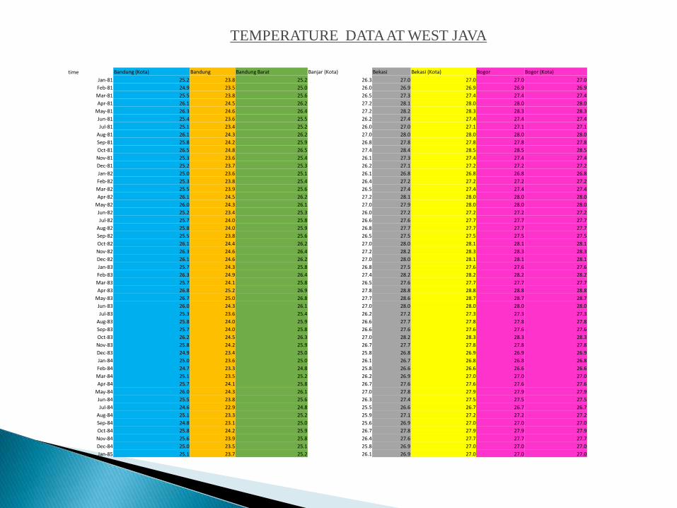
STAR Model of Cliff-Ord (1975)
Prod . Welli (t) = 00 Prod. Welli (t) +
11 wij Prod.Wellj (t-1) + Error Welli (t)
STAR Model of Pfeifer (1979)
Prod . Welli (t) = 01 Prod. Welli (t-1) +
11 wij Prod.Wellj (t-1) + Error Welli ( t)

The weight matrix to describe the
characteristic of locations
To estimate the parameters model
To determine the least squares
properties of estimators
LACK OF THE STAR MODEL JUST ONLY APPLICABLE FOR HOMOGENOUS LOCATIONS

Source: Siregar [20]
Dual Porosity from Matrix and Fracturer
0 50 100 150
50
01
00
01
50
02
00
02
50
03
00
0
Data Produksi JTB68


Semivariogram
The semivariogram is a graphical device for
modelling spatial continuity. The spatial
process is assumed to hold intrinsic hypothesis:
for h a vector in R2, we have:
E[Y(s+h)-Y(s)]=0
E[Y(s+h)-Y(s)]2= 2(h)
The quantity 2(h) which is a function only the
increment h is known as the variogram [(h)
has been called semivariogram] and is the
crucial parameter of spatial processes

Estimation of Semivariogram
Under the constant mean assumption, E[Y(s)]=m, so a natural estimation of the
semivariogram is defined (Cressie, 1993):
for h >0 and N(h) is number of pairs of locations (si,sj) with d(si-sj) h and d is
distance.
2
),(d:),(
)]()([)(N2
1)(ˆ
jiji
hssss
ssh
h ji YY

Theoretical Model of Semivariogram
The spherical model probably the most commonly used model. It is presented as:
where c is sill or variance of observations and a is range.
ah,c
ah,/a)0.5(h)/a1.5(hc)(hγ
ij
ij3
ijijij
][ˆ

The Spatial Weights using the Semivariogram
N)h(w
i,1hw
tan,
,
N
1i
N
1j
ijss
N
1j
ijss
)(
weightspatiallydardizedsthe
ji,0
ji,A
a
)(hw
aA
weightspatiallyoriginalthe
ji,0
ji,
)](hγ[1
1
a
ij
ij
ijss
N
ij
ijij
ij
^
ij

Ruchjana (2002)
Based on the oil production phenomenon at volcanic layer at West Java are heterogeneous
Prod . Welli (t) = (i)01 Prod. Welli (t-1)
+ (i)11 wij Prod.Wellj (t-1) + Error Welli (t)
the autoregressive and space time parameters are different for each well

Generalized Spatial Time AutoRegressive order one Model,
GSTAR(1;1)
)()1(),,()1(),,(
)()1()1()(
)1()(
11
)1(
11
)(
01
)1(
01
)1()1(
)1()(
)1(
)(11)1()(01)1(
ttdiagtdiag
tttt
NN
NxNxNxNNxNNxNxNNx
ezWz
ezWzz
01 : diagonal matrices containing the autoregressive parameter at time lag 1
11 : diagonal matrices containing the spatial-time parameter at spatial lag 1
and time lag 1
z(t) : the random vector of observation at time t
W(1) : the weight matrix at spatial lag 1
e(t) ~ iid (0, 2IN)

GSTAR(1;1) Model
For locatons i =1,2,…,N at time t :
)(
)(
)1(
)1(
)1(0
0
)1(
)1(
0
0
)(
)( 11
)1(
1
)1(
1
)1(
11
)(
11
)1(
111
)(
01
)1(
011
te
te
tz
tz
ww
ww
tz
tz
tz
tz
NNNNN
N
N
N
N
N
GSTAR(1;1) model can be written as VAR(1):
)()1()( ttt ezz
][ )1(
1101 W
We can use the least square method to estimate the parameter GSTAR(1;1)

N
j
jNj
N
j
jj
N
j
jj
N
N
tzw
tzw
tzw
ttt
G
1
)1(
1
)1(
2
1
)1(
1
)(
11
)1(
11
)(
01
)1(
01
)1(00
00
0)1(0
00)1(
where
)(diag)1(diag)(
2
V
eVzz
X
(V.1)
The space time software still not yet provide
We built the GSTAR Script S-Plus to estimate the parameters using least squares method, for order 1, 2, …, p in time and order 1, 2, …, p in space.


The GSTAR(2;1) using binary weights gave the better result than STAR(1;1) or GSTAR(1;1) with binary and uniform weights, it has AIC minimum

Mesosphere
Ionosphere/
Thermosphee
Stratosphere
Troposphere
Collaboration with the
Center for Application at
Atmospheric Science and
Climate of National Institute
of Aeronautics and Space
(LAPAN), Bandung
Equatorial Atmospheric Radar (Padang)

Application of STAR(1;1) and
GSTAR(1;1) Models to Oil Production
The Jatibarang Field is located near
Cirebon, West Java-Indonesia. The
reservoir formation is a fractured volcanic
rock.
We use the monthly oil production data
from 3 wells in 80 observations: JTB68,
JTB72 and Jtb120.

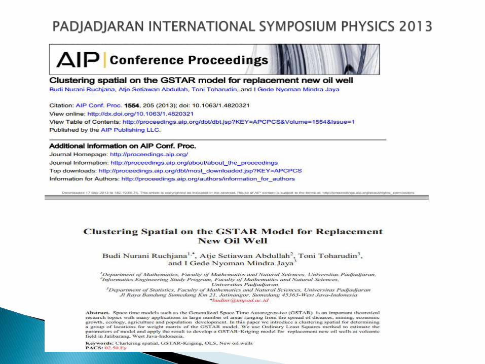
Application STAR and GSTAR model in Petroleum Field, Volcanic Layer-West Java
Collaboration between Unpad, ITB, TU Delft, Pertamina since 1999-now, and Chevron Indonesia Company


Production Correlation Data
between 2 wells (185 months)
Well JTB68 JTB72 JTB120
JTB68 1
JTB72 0.414 1
JTB120 0.547 0.456 1
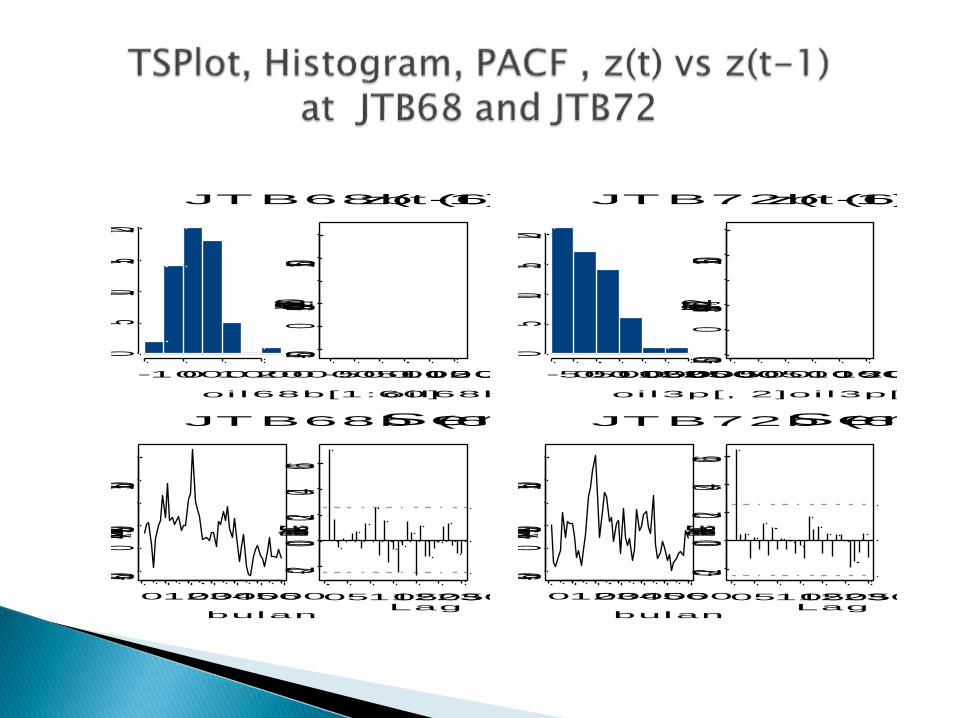
-10000 10002000
05
1015
20
oil68b[1:60]
JTB68b (60obs)
oil68b[1:59]
oil68b[2:60]
-5000500100015002000
-500050
01500
z(t-1) vs z(t) Jtb68b
bulan
z(t) (m3/hari)
0102030405060
-500050
01500
JTB68b (60obs)
Lag
Partial ACF
051015202530
-0.20.0
0.20.4
0.6
Series : oil3p[, 1]
-50005001000150020002500
05
1015
20
oil3p[, 2]
JTB72b (60obs)
oil3p[1:59, 2]
oil3p[2:60, 2]
-5000500100015002000
-5000
5001500
z(t-1) vs z(t) Jtb72b
bulan
z(t) (m3/hari)
0102030405060
-500050
01500
JTB72b (60obs)
Lag
Partial ACF
051015202530
-0.20.0
0.20.4
0.6
Series : oil3p[, 2]

18
The uniform weight matrix Wu , the spatial weight matrix Ws
using the thickness data of 83 wells
úúú
û
ù
êêê
ë
é
úúú
û
ù
êêê
ë
é
úúú
û
ù
êêê
ë
é
0462.0538.0
452.00548.0
490.0510.00
0000657.0000797.0
000657.00000766.0
000797.0000766.00
05.05.0
5.005.0
5.05.00
s
s
u
W
W
W

Wells Well1 Well2 Well3
Well1 71,50 1,80 9,10
Well2 10,20 71,50 8,40
Well3 10,00 8,60 71,50
715.0086.0100.0
084.0715.0102.0
091.0018.0715.0
ˆ

Wells Well1 Well2 Well3
Well1 62,20 15,70 15,10
Well2 12,22 63,80 10,08
Well3 0,02 0,01 83,90
MonthlyP
rod
uctio
n0 50 100 150
01
00
02
00
03
00
0Monthly
Pro
du
ctio
n0 50 100 150
01
00
02
00
03
00
0Monthly
Pro
du
ctio
n0 50 100 150
01
00
02
00
03
00
0
z1(t)z1hat(t)r1(t)
Fitted GSTAR Well1

Least Squares Estimator of GSTAR(1;1) Ws
Well )(10ˆ i )(
11ˆ i SSE Total
SSE
MAPE Total
MAPE
JTB68
b
0.623
(0.108)
0.308
(0.114)
6,361
x 106
1,048 %
JTB72
b
0.638
(0.094)
0.223
(0.101)
9,504
x 106
21,360
x 106
1,494 %
3,223 %
JTB12
0b
0.839
(0.084)
0.028
(0.115)
5,495
x 106
0,681 %

)3(11
)2(11
)1(11
11)3(
10
)2(10
)1(10
10
1110
ˆ00
0ˆ0
00ˆ
ˆ,
ˆ00
0ˆ0
00ˆ
ˆ,)()(~
)1(~ˆ)1(~ˆ)(~̂
or
zzz
zWzz
tt
ttt s
)49(ˆ
)49(ˆ
)49(ˆ
0462,0538,0
452,00548,0
490,0510,00
028,000
0223,00
00308,0
)49(ˆ
)49(ˆ
)49(ˆ
839,000
0638,00
00622,0
)50(ˆ
)50(ˆ
)50(ˆ
50
3
2
1
3
2
1
3
2
1
z
z
z
z
z
z
z
z
z
t

Sufficient Conditions for the GSTAR(1;1) stationary
If for all locations, i =1, 2 ,…,N, theparameters and satisfies)(
10i
)(11
i
1,1 )(
11
)(
10
)(
11
)(
10 iiii
then the GSTAR(1;1) model is
stationary process.

GSTAR KRIGING
The coordinate’s position of ten excluding sample locations between two oil wells (JTB68 and JTB72)
Using the (i)10 and (i)
11 parameters, we can simulate the
GSTAR(1;1) for ten excluding sample locations, and we have the model for prediction of oil production for each new oil
well.
Well's coordinate
0
100
200
300
400
14000 14050 14100 14150 14200 14250 14300 14350 14400
X
Y

)(
11is
322430003224320032243400322436003224380032244000322442003224440032244600
21950000 21952000 21954000
Y
X
Koordinat Sumur Minyak

J. Bruining
H. P. Lopuhaä
Budi Nurani Ruchjana
Asep K. Permadi
Sutawanir Darwis
*) Research is funded by KNAW the Netherlands
through Mobility Programme 2007 and General
Manager Deepwater Project, Chevron Indonesia
Company, Chevron IndoAsia Business
Oil Well Placement Design through Geostatistical Analysis using the Generalized Space Time Autoregressive (GSTAR) Kriging Model *)

GSTAR(1;1) model
1. (t) has zero mean and constant of variance-
covariance matrix
2. (t) doesn’t have a correlation with error in the last
time
3. There is no autocorrelation between error in
location at time t : i(t) dan j(t) , ij = 0
4. (t) is identically independent normal
GSTAR(1,1)-ARCH(1) MODEL (NAINGGOLAN, 2011)
• New error assumption: heteroscedasticity of variance covariance matrix
10 11( ) ( 1) ( 1) ( )t t t t Z Z W Z ε
2( ( ) ~ (0, )iid
Nt N ε I
2
1 12 1
2
21 2 2
1
2
1 2
( ) ( ) ( )
( ) ( ) ( )( ( ) )
( ) ( ) ( )
N
N
t t
N N N
t t t
t t tVar t F
t t t
ε Σ
2
1 0 0
0 1 0( ( ))
0 0 1
Var t
ε

( ) ( )
01 11( ) ( 1) ( ) ( )i i
i i i i it t t t z μ Φ z Φ V ε
( ) ( ) ( )
01 11
z (1) z (0) (0) ε (1)1
z (2) z (1) (1) ε (2)1, , , , ,
z ( ) z ( 1) ( 1) ε ( )1
i i i i
i i i ii i i
i i i i
i i i iT T T T
é ù é ù é ùê ú ê ú ê úê ú ê ú ê ú ê ú ê ú ê úê ú ê ú ê ú
ë û ë û ë û
V
VX ε
V
y
)()1( tt
where
iVzX

autocorrelation
error ≠ 0
11 12 13 14 15
21 22 23 24 25
31 32 33 33 35
41 42 43 44 45
51 52 53 54 55
( )Var
ε
Error Variance
between location is
heteroscedasticity
2
2
2 2
2
2
0 0 0 0
0 0 0 0
( ) 0 0 0 0
0 0 0 0
0 0 0 0
Var
ε I

GSTAR-SUR in Linear Model
y = Xβ+ε
where
1
2
1011 11
11 1
201 21 1 1 21
2 2 2
22 2
1 10
; ;
M
KT T
KT T
M M M
M MM
MT MMK
y
y
y
y
y
y
é ùé ùê úê úê úê úê úê úê úê ú
é ù é ù é ùê úê úê ú ê ú ê úê úê úê ú ê ú ê úê ú ê úê ú ê ú ê úê úê úê ú ê ú ê úê úê úë û ë û ë ûê úê ú
ê úê úê úê úê úê úê úê úë û ë û
y
y
y
y
T
é ùê úê úê úê úê úê úê úê úê úê úê úê úê úê úë û
é ùê úê úê úê úë û
1
2
M
X 0 0
0 X 0X
0 0 X


This paper introduces a novel model - GeneralizedSpace-Time Autoregressive Integrated MovingAverage (GSTARIMA) methodology - into the field ofshort-term traffic flow forecasting in urban network.Compared to traditional STARIMA, GSTARIMA is amore flexible model class where parameters aredesigned to vary per location.
GSTARIMA-X model and its applications?
Sahid, Ph.D student at Graduate Program ITS

The space time models, especially STAR, and GSTAR models are informed.
The application of the space time models are shown.
The continuation research on space time models are introduced
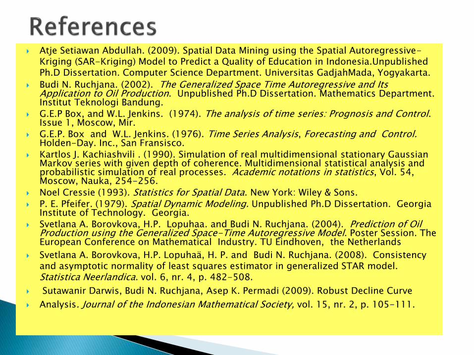
Atje Setiawan Abdullah. (2009). Spatial Data Mining using the Spatial Autoregressive-Kriging (SAR-Kriging) Model to Predict a Quality of Education in Indonesia.Unpublished Ph.D Dissertation. Computer Science Department. Universitas GadjahMada, Yogyakarta.
Budi N. Ruchjana. (2002). The Generalized Space Time Autoregressive and Its Application to Oil Production. Unpublished Ph.D Dissertation. Mathematics Department. Institut Teknologi Bandung.
G.E.P Box, and W.L. Jenkins. (1974). The analysis of time series: Prognosis and Control. Issue 1, Moscow, Mir.
G.E.P. Box and W.L. Jenkins. (1976). Time Series Analysis, Forecasting and Control. Holden-Day. Inc., San Fransisco.
Kartlos J. Kachiashvili . (1990). Simulation of real multidimensional stationary Gaussian Markov series with given depth of coherence. Multidimensional statistical analysis and probabilistic simulation of real processes. Academic notations in statistics, Vol. 54, Moscow, Nauka, 254-256.
Noel Cressie (1993). Statistics for Spatial Data. New York: Wiley & Sons.
P. E. Pfeifer. (1979). Spatial Dynamic Modeling. Unpublished Ph.D Dissertation. Georgia Institute of Technology. Georgia.
Svetlana A. Borovkova, H.P. Lopuhaa. and Budi N. Ruchjana. (2004). Prediction of Oil Production using the Generalized Space-Time Autoregressive Model. Poster Session. The European Conference on Mathematical Industry. TU Eindhoven, the Netherlands
Svetlana A. Borovkova, H.P. Lopuhaä, H. P. and Budi N. Ruchjana. (2008). Consistency and asymptotic normality of least squares estimator in generalized STAR model. Statistica Neerlandica. vol. 6, nr. 4, p. 482-508.
Sutawanir Darwis, Budi N. Ruchjana, Asep K. Permadi (2009). Robust Decline Curve
Analysis. Journal of the Indonesian Mathematical Society, vol. 15, nr. 2, p. 105-111.

ASSMS-Lahore-Pakistan 2008