Aswath Damodaran1 The Investment Principle Aswath Damodaran Stern School of Business

Aswath Damodaran 1

The Investment Principle

Aswath Damodaran

Stern School of Business

Aswath Damodaran 2

First Principles

Invest in projects that yield a return greater than the minimum acceptable hurdle rate.• The hurdle rate should be higher for riskier projects and reflect the

financing mix used - owners’ funds (equity) or borrowed money (debt)

• Returns on projects should be measured based on cash flows generated and the timing of these cash flows; they should also consider both positive and negative side effects of these projects.

Choose a financing mix that minimizes the hurdle rate and matches the assets being financed.

If there are not enough investments that earn the hurdle rate, return the cash to stockholders.• The form of returns - dividends and stock buybacks - will depend upon

the stockholders’ characteristics.

Aswath Damodaran 3

What is a investment or a project?

Any decision that requires the use of resources (financial or otherwise) is a project.

Broad strategic decisions• Entering new areas of business• Entering new markets• Acquiring other companies

Tactical decisions Management decisions

• The product mix to carry• The level of inventory and credit terms

Decisions on delivering a needed service• Lease or buy a distribution system• Creating and delivering a management information system

Aswath Damodaran 4

Measuring Returns Right: The Basic Principles

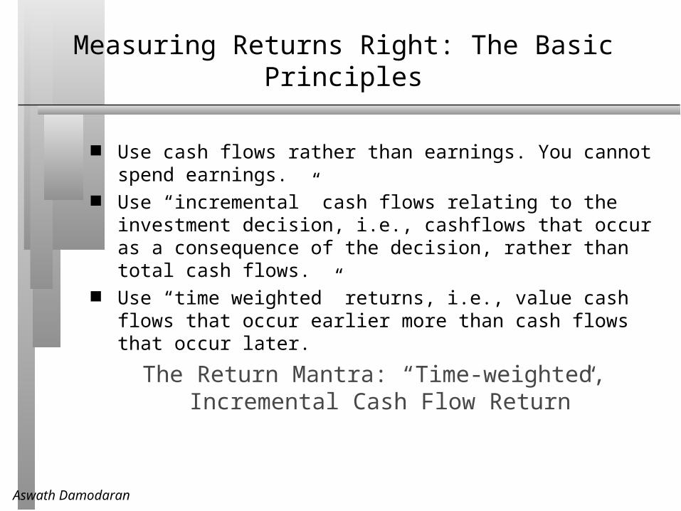
Use cash flows rather than earnings. You cannot spend earnings. Use “incremental” cash flows relating to the investment decision, i.e.,

cashflows that occur as a consequence of the decision, rather than total cash flows.

Use “time weighted” returns, i.e., value cash flows that occur earlier more than cash flows that occur later.

The Return Mantra: “Time-weighted, Incremental Cash Flow Return”

Aswath Damodaran 5

Steps in Investment Analysis

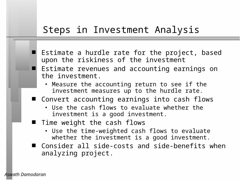
Estimate a hurdle rate for the project, based upon the riskiness of the investment

Estimate revenues and accounting earnings on the investment.• Measure the accounting return to see if the investment measures up to the

hurdle rate. Convert accounting earnings into cash flows

• Use the cash flows to evaluate whether the investment is a good investment.

Time weight the cash flows• Use the time-weighted cash flows to evaluate whether the investment is a

good investment. Consider all side-costs and side-benefits when analyzing project.

Aswath Damodaran 6

I. Estimating Discount Rates

Aswath Damodaran 7

The Essence of Discount Rates: The notion of a benchmark

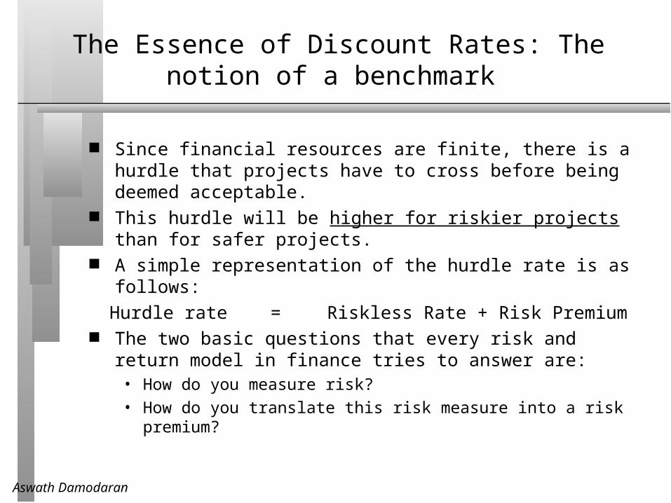
Since financial resources are finite, there is a hurdle that projects have to cross before being deemed acceptable.

This hurdle will be higher for riskier projects than for safer projects. A simple representation of the hurdle rate is as follows:

Hurdle rate = Riskless Rate + Risk Premium The two basic questions that every risk and return model in finance

tries to answer are:• How do you measure risk?

• How do you translate this risk measure into a risk premium?

Aswath Damodaran 8

1. The Nominal versus Real Choice & A Currency for your analysis

A project can be analyzed in nominal terms (in which case inflation is incorporated into both your cashflows and your discount rate) or in real terms. When inflation is high and volatile, analysts may find it easier to do everything in real terms.

If an analysis is nominal, you have to pick the currency to do the analysis is. Any project can be analyzed in any currency. In choosing a currency to do the analysis, you should consider:• Where the project will be located and what currency its costs and

revenues will be in. (The costs may be in one currency and the revenues may be in another or more than one currency)

• How easy it will be to obtain fundamental information on risk free rates and risk premiums in that currency.

Aswath Damodaran 9

2. Risk Free Rate

For an investment to be risk free, it has to fulfill two conditions:• There can have no default risk

• There can be no reinvestment risk Using this principle strictly, there can be no one risk free rate for any

investment that delivers cash flows at different points in time. The right risk free rate for each cash flow will be the interest rate on a zero-coupon default free government bond maturity on the same date as the cash flow.

Aswath Damodaran 10

Some common sense rules on risk free rates

Currency with default free entity: If you are working with a currency where a default free entity exists ($ or Euro), use the interest rate on a government bond with roughly the same duration as the project as the riskfree rate for all cashflows.

Currency with no default free entity: There are two solutions when there is no default free entity:

• Approach 1: Subtract default spread from local government bond rate:Government bond rate in local currency terms - Default spread for Government in local

currency• Approach 2: Use forward rates and the riskless rate in an index currency (say Euros

or dollars) to estimate the riskless rate in the local currency. Real Risk free rate: To obtain a real riskfree rate, you can try the following:

• from an inflation-indexed government bond, if one exists• set equal, approximately, to the long term real growth rate of the economy in which

the valuation is being done.

Aswath Damodaran 11

3. Determine a debt ratio and a cost of debt for the project

Most projects do not carry debt on their own. Instead, the parent company borrows money, using its general assets as collateral, and uses this money to fund the projects.

Some projects are large enough and have assets that are separable from the firm. These projects sometimes borrow on their own assets, with no recourse against the parent company.

Aswath Damodaran 12

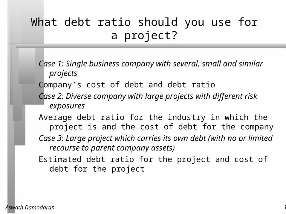
What debt ratio should you use for a project?

Case 1: Single business company with several, small and similar projects

Company’s cost of debt and debt ratio

Case 2: Diverse company with large projects with different risk exposures

Average debt ratio for the industry in which the project is and the cost of debt for the company

Case 3: Large project which carries its own debt (with no or limited recourse to parent company assets)

Estimated debt ratio for the project and cost of debt for the project

Aswath Damodaran 13

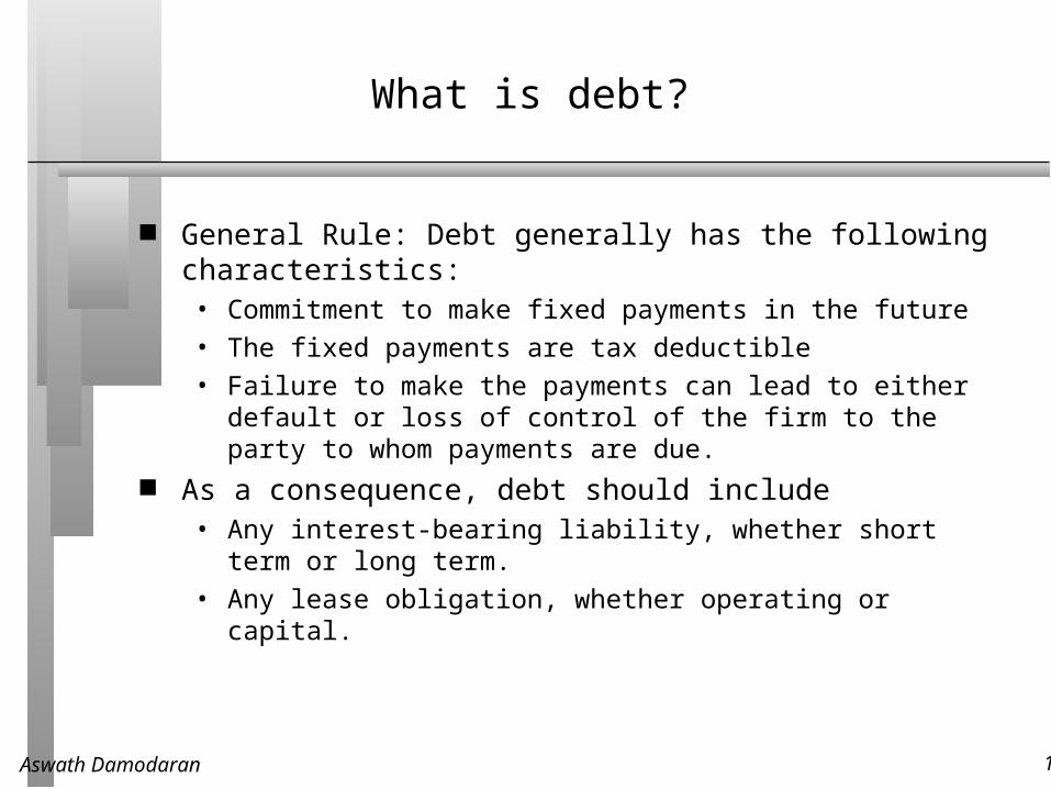
What is debt?

General Rule: Debt generally has the following characteristics:• Commitment to make fixed payments in the future

• The fixed payments are tax deductible

• Failure to make the payments can lead to either default or loss of control of the firm to the party to whom payments are due.

As a consequence, debt should include• Any interest-bearing liability, whether short term or long term.

• Any lease obligation, whether operating or capital.

Aswath Damodaran 14

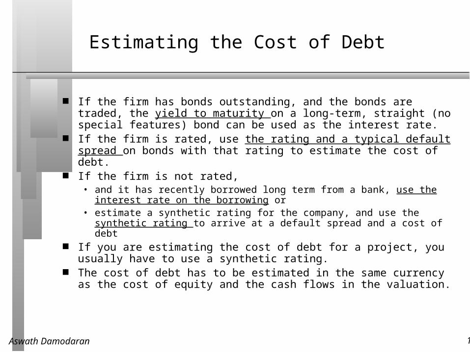
Estimating the Cost of Debt

If the firm has bonds outstanding, and the bonds are traded, the yield to maturity on a long-term, straight (no special features) bond can be used as the interest rate.

If the firm is rated, use the rating and a typical default spread on bonds with that rating to estimate the cost of debt.

If the firm is not rated, • and it has recently borrowed long term from a bank, use the interest rate

on the borrowing or• estimate a synthetic rating for the company, and use the synthetic rating to

arrive at a default spread and a cost of debt If you are estimating the cost of debt for a project, you usually have to

use a synthetic rating. The cost of debt has to be estimated in the same currency as the cost

of equity and the cash flows in the valuation.

Aswath Damodaran 15

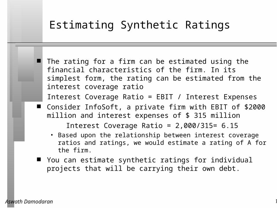
Estimating Synthetic Ratings

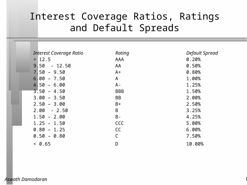
The rating for a firm can be estimated using the financial characteristics of the firm. In its simplest form, the rating can be estimated from the interest coverage ratio

Interest Coverage Ratio = EBIT / Interest Expenses Consider InfoSoft, a private firm with EBIT of $2000 million and

interest expenses of $ 315 million

Interest Coverage Ratio = 2,000/315= 6.15• Based upon the relationship between interest coverage ratios and ratings,

we would estimate a rating of A for the firm. You can estimate synthetic ratings for individual projects that will be

carrying their own debt.

Aswath Damodaran 16

Interest Coverage Ratios, Ratings and Default Spreads

Interest Coverage Ratio Rating Default Spread> 12.5 AAA 0.20%9.50 - 12.50 AA 0.50%7.50 – 9.50 A+ 0.80%6.00 – 7.50 A 1.00%4.50 – 6.00 A- 1.25%3.50 – 4.50 BBB 1.50%3.00 – 3.50 BB 2.00%2.50 – 3.00 B+ 2.50%2.00 - 2.50 B 3.25%1.50 – 2.00 B- 4.25%1.25 – 1.50 CCC 5.00%0.80 – 1.25 CC 6.00%0.50 – 0.80 C 7.50%

< 0.65 D 10.00%

Aswath Damodaran 17

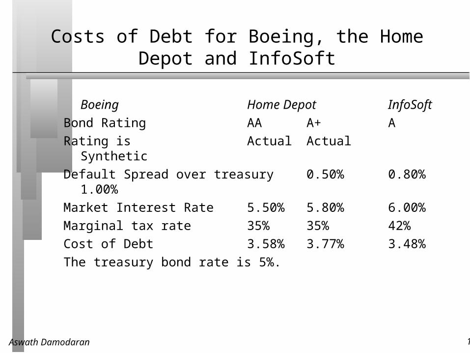
Costs of Debt for Boeing, the Home Depot and InfoSoft

Boeing Home Depot InfoSoft

Bond Rating AA A+ A

Rating is Actual Actual Synthetic

Default Spread over treasury 0.50% 0.80% 1.00%

Market Interest Rate 5.50% 5.80% 6.00%

Marginal tax rate 35% 35% 42%

Cost of Debt 3.58% 3.77% 3.48%

The treasury bond rate is 5%.

Aswath Damodaran 18

4. Cost of Equity

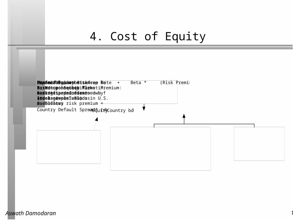
Cost of Equity = Riskfree Rate + Beta * (Risk Premium)Has to be in the samecurrency as cash flows, and defined in same terms(real or nominal) as thecash flows

Preferably, a bottom-up beta,based upon other firms in thebusiness, and firm’s own financialleverage

Historical Premium1. Mature Equity Market Premium:Average premium earned bystocks over T.Bonds in U.S.2. Country risk premium =

Country Default Spread* ( σEquity/σCountry bond)

Implied PremiumBased on how equitymarket is priced todayand a simple valuationmodel

or

Aswath Damodaran 19

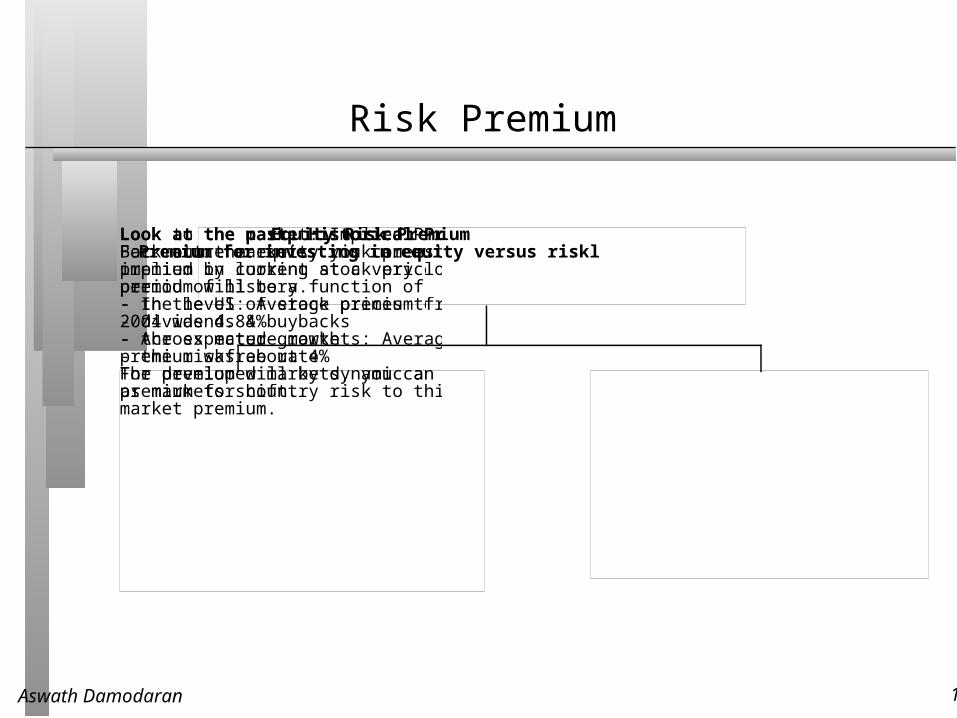
Risk Premium

Equity Risk PremiumPremium for investing in equity versus riskless asset

Look at the past: Historical PremiumFor mature markets, you can estimate the premium by looking at a very long time period of history.- In the US: Average premium from 1928-2004 was 4.84%- Across mature markets: Average premium was about 4%For developed markets, you can add a premium for country risk to this mature market premium.

Look to the market: Implied PremiumBack out the equity risk premium that is implied in current stock prices. This premium will be a function of- the level of stock prices today- dividends & buybacks - the expected growth- the riskfree rateThe premium will by dynamic and shift as markets shift.

Aswath Damodaran 20

Everyone uses historical premiums, but..

The historical premium is the premium that stocks have historically earned over riskless securities.

Practitioners never seem to agree on the premium; it is sensitive to • How far back you go in history…• Whether you use T.bill rates or T.Bond rates• Whether you use geometric or arithmetic averages.

For instance, looking at the US:Arithmetic average Geometric Average

Stocks - Stocks - Stocks - Stocks -Historical Period T.Bills T.Bonds T.Bills T.Bonds1928-2002 7.67% 6.25% 5.73% 4.53%1962-2002 5.17% 3.66% 3.90% 2.76%1992-2002 6.32% 2.15% 4.69% 0.95%

Aswath Damodaran 21

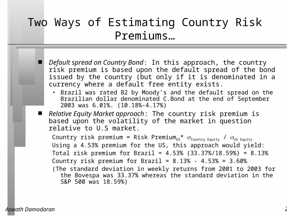
Two Ways of Estimating Country Risk Premiums…

Default spread on Country Bond: In this approach, the country risk premium is based upon the default spread of the bond issued by the country (but only if it is denominated in a currency where a default free entity exists.

• Brazil was rated B2 by Moody’s and the default spread on the Brazilian dollar denominated C.Bond at the end of September 2003 was 6.01%. (10.18%-4.17%)

Relative Equity Market approach: The country risk premium is based upon the volatility of the market in question relative to U.S market.

Country risk premium = Risk PremiumUS* σCountry Equity / σUS Equity

Using a 4.53% premium for the US, this approach would yield:Total risk premium for Brazil = 4.53% (33.37%/18.59%) = 8.13%Country risk premium for Brazil = 8.13% - 4.53% = 3.60%(The standard deviation in weekly returns from 2001 to 2003 for the Bovespa was

33.37% whereas the standard deviation in the S&P 500 was 18.59%)

Aswath Damodaran 22

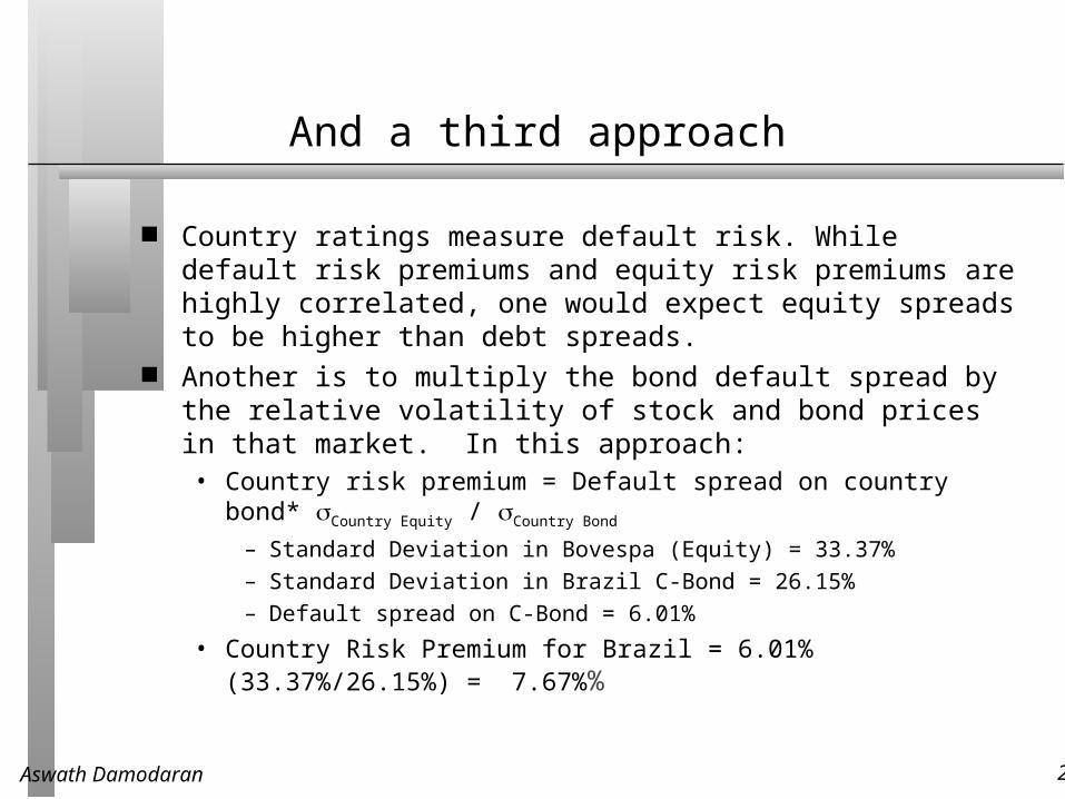
And a third approach

Country ratings measure default risk. While default risk premiums and equity risk premiums are highly correlated, one would expect equity spreads to be higher than debt spreads.

Another is to multiply the bond default spread by the relative volatility of stock and bond prices in that market. In this approach:• Country risk premium = Default spread on country bond* σCountry Equity /

σCountry Bond

– Standard Deviation in Bovespa (Equity) = 33.37%

– Standard Deviation in Brazil C-Bond = 26.15%

– Default spread on C-Bond = 6.01%

• Country Risk Premium for Brazil = 6.01% (33.37%/26.15%) = 7.67%%

Aswath Damodaran 23

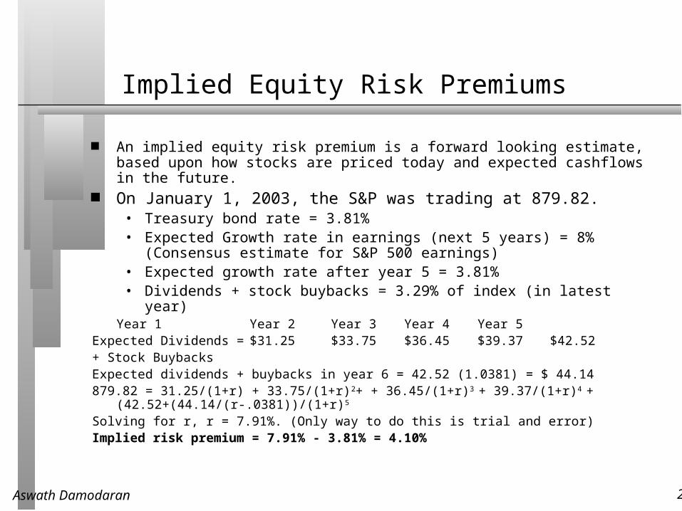
Implied Equity Risk Premiums

An implied equity risk premium is a forward looking estimate, based upon how stocks are priced today and expected cashflows in the future.

On January 1, 2003, the S&P was trading at 879.82.• Treasury bond rate = 3.81%• Expected Growth rate in earnings (next 5 years) = 8% (Consensus estimate for S&P

500 earnings)• Expected growth rate after year 5 = 3.81%• Dividends + stock buybacks = 3.29% of index (in latest year)

Year 1 Year 2 Year 3 Year 4 Year 5

Expected Dividends = $31.25 $33.75 $36.45 $39.37 $42.52

+ Stock BuybacksExpected dividends + buybacks in year 6 = 42.52 (1.0381) = $ 44.14879.82 = 31.25/(1+r) + 33.75/(1+r)2+ + 36.45/(1+r)3 + 39.37/(1+r)4 + (42.52+(44.14/(r-.0381))/(1+r)5

Solving for r, r = 7.91%. (Only way to do this is trial and error)Implied risk premium = 7.91% - 3.81% = 4.10%

Aswath Damodaran 24

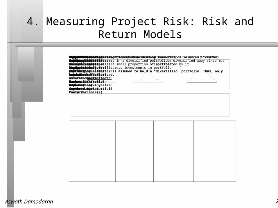
4. Measuring Project Risk: Risk and Return Models

The risk in an investment can be measured by the variance in actual returns around an expected returnE(R)Riskless InvestmentLow Risk InvestmentHigh Risk InvestmentE(R)E(R)Risk that is specific to investment (Firm Specific) Risk that affects all investments (Market Risk)Can be diversified away in a diversified portfolio Cannot be diversified away since most assets1. each investment is a small proportion of portfolio are affected by it.2. risk averages out across investments in portfolioThe marginal investor is assumed to hold a “diversified” portfolio. Thus, only market risk will be rewarded and priced.

The CAPMThe APMMulti-Factor ModelsProxy ModelsIf there is 1. no private information2. no transactions costthe optimal diversified portfolio includes everytraded asset. Everyonewill hold this market portfolioMarket Risk = Risk added by any investment to the market portfolio:

If there are no arbitrage opportunities then the market risk ofany asset must be captured by betas relative to factors that affect all investments.Market Risk = Risk exposures of any asset to market factors

Beta of asset relative toMarket portfolio (froma regression)

Betas of asset relativeto unspecified marketfactors (from a factoranalysis)

Since market risk affectsmost or all investments,it must come from macro economic factors.Market Risk = Risk exposures of any asset to macro economic factors.

Betas of assets relativeto specified macroeconomic factors (froma regression)

In an efficient market,differences in returnsacross long periods mustbe due to market riskdifferences. Looking forvariables correlated withreturns should then give us proxies for this risk.Market Risk = Captured by the Proxy Variable(s)

Equation relating returns to proxy variables (from aregression)

Step 1: Defining RiskStep 2: Differentiating between Rewarded and Unrewarded RiskStep 3: Measuring Market Risk

Aswath Damodaran 25

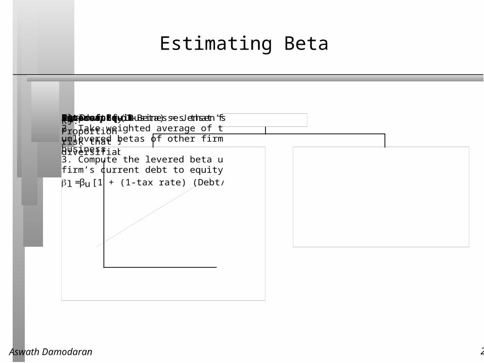
Estimating Beta

Beta of EquityRjRmSlope = BetaIntercept - Rf (1-Beta) = Jensen’s AlphaTop-DownBottom-up1. Identify businesses that firm is in.2. Take weighted average of theunlevered betas of other firms in thebusiness 3. Compute the levered beta using thefirm’s current debt to equity ratio:

βl = βu [1 + (1-tax rate) (Debt/Equity)]

R2: Proportion of risk that is not diversifiable

Aswath Damodaran 26

Decomposing Boeing’s Beta

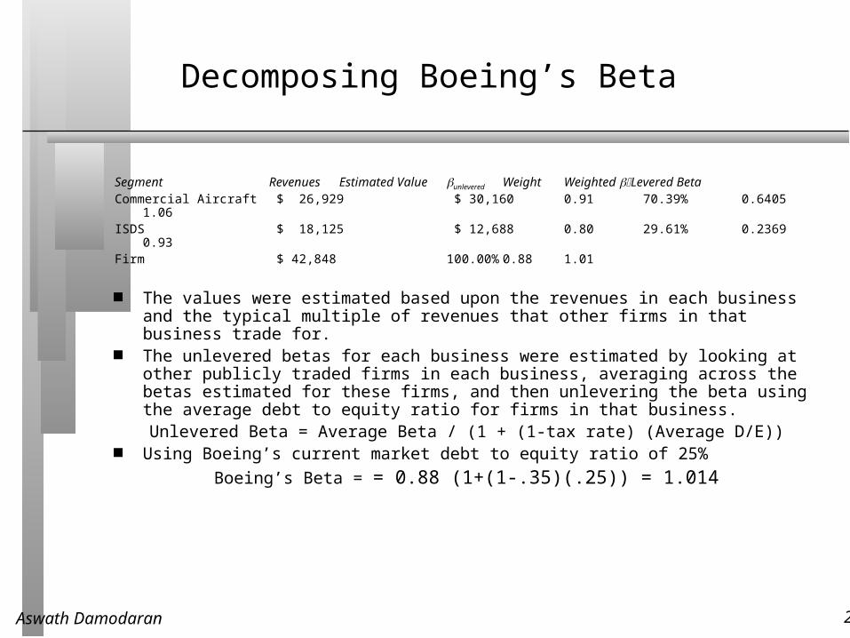
Segment Revenues Estimated Value βunlevered Weight Weighted βLevered BetaCommercial Aircraft $ 26,929 $ 30,160 0.91 70.39% 0.6405 1.06ISDS $ 18,125 $ 12,688 0.80 29.61% 0.2369 0.93Firm $ 42,848 100.00% 0.88 1.01

The values were estimated based upon the revenues in each business and the typical multiple of revenues that other firms in that business trade for.

The unlevered betas for each business were estimated by looking at other publicly traded firms in each business, averaging across the betas estimated for these firms, and then unlevering the beta using the average debt to equity ratio for firms in that business.

Unlevered Beta = Average Beta / (1 + (1-tax rate) (Average D/E)) Using Boeing’s current market debt to equity ratio of 25%

Boeing’s Beta = = 0.88 (1+(1-.35)(.25)) = 1.014

Aswath Damodaran 27

The Home Depot’s Comparable Firms

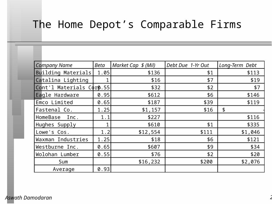
Company Name Beta Market Cap $ (Mil) Debt Due 1-Yr Out Long-Term DebtBuilding Materials 1.05 $136 $1 $113Catalina Lighting 1 $16 $7 $19Cont'l Materials Corp 0.55 $32 $2 $7Eagle Hardware 0.95 $612 $6 $146Emco Limited 0.65 $187 $39 $119Fastenal Co. 1.25 $1,157 $16 $ - HomeBase Inc. 1.1 $227 $116Hughes Supply 1 $610 $1 $335Lowe's Cos. 1.2 $12,554 $111 $1,046Waxman Industries 1.25 $18 $6 $121Westburne Inc. 0.65 $607 $9 $34Wolohan Lumber 0.55 $76 $2 $20

Sum $16,232 $200 $2,076Average 0.93

Aswath Damodaran 28

Estimating The Home Depot’s Bottom-up Beta

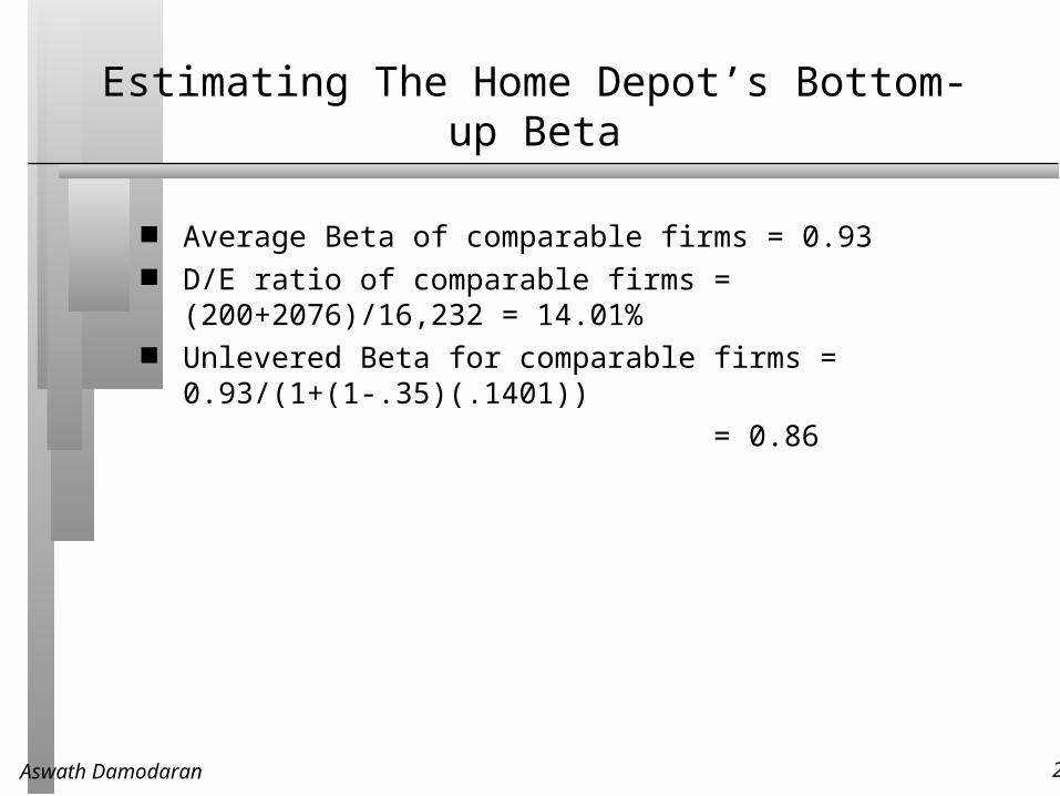
Average Beta of comparable firms = 0.93 D/E ratio of comparable firms = (200+2076)/16,232 = 14.01% Unlevered Beta for comparable firms = 0.93/(1+(1-.35)(.1401))

= 0.86

Aswath Damodaran 29

Beta for InfoSoft, a Private Software Firm

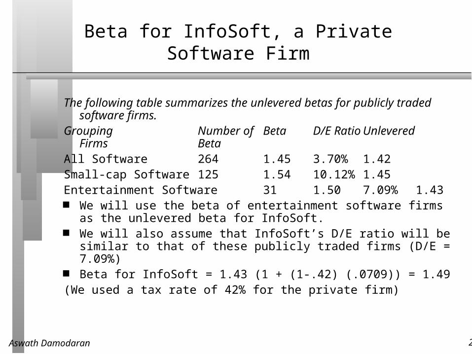
The following table summarizes the unlevered betas for publicly traded software firms.

Grouping Number of Beta D/E Ratio Unlevered Firms Beta

All Software 264 1.45 3.70% 1.42Small-cap Software 125 1.54 10.12% 1.45Entertainment Software 31 1.50 7.09% 1.43 We will use the beta of entertainment software firms as the unlevered

beta for InfoSoft. We will also assume that InfoSoft’s D/E ratio will be similar to that of

these publicly traded firms (D/E = 7.09%) Beta for InfoSoft = 1.43 (1 + (1-.42) (.0709)) = 1.49(We used a tax rate of 42% for the private firm)

Aswath Damodaran 30

Total Risk versus Market Risk

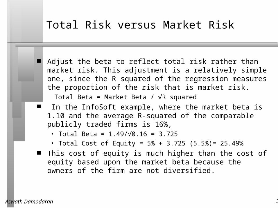
Adjust the beta to reflect total risk rather than market risk. This adjustment is a relatively simple one, since the R squared of the regression measures the proportion of the risk that is market risk. Total Beta = Market Beta / √R squared

In the InfoSoft example, where the market beta is 1.10 and the average R-squared of the comparable publicly traded firms is 16%,• Total Beta = 1.49/√0.16 = 3.725

• Total Cost of Equity = 5% + 3.725 (5.5%)= 25.49% This cost of equity is much higher than the cost of equity based upon

the market beta because the owners of the firm are not diversified.

Aswath Damodaran 31

Estimating a beta for a project

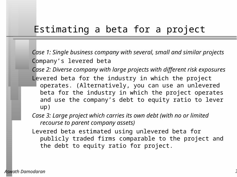
Case 1: Single business company with several, small and similar projects

Company’s levered beta

Case 2: Diverse company with large projects with different risk exposures

Levered beta for the industry in which the project operates. (Alternatively, you can use an unlevered beta for the industry in which the project operates and use the company’s debt to equity ratio to lever up)

Case 3: Large project which carries its own debt (with no or limited recourse to parent company assets)

Levered beta estimated using unlevered beta for publicly traded firms comparable to the project and the debt to equity ratio for project.

Aswath Damodaran 32

5. Cost of Capital

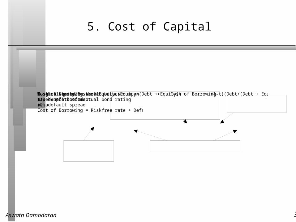
Cost of Capital = Cost of Equity (Equity/(Debt + Equity)) + Cost of Borrowing (1-t) (Debt/(Debt + Equity))Cost of borrowing should be based upon(1) synthetic or actual bond rating(2) default spreadCost of Borrowing = Riskfree rate + Default spread

Marginal tax rate, reflectingtax benefits of debtWeights should be market value weightsCost of equitybased upon bottom-upbeta

Aswath Damodaran 33

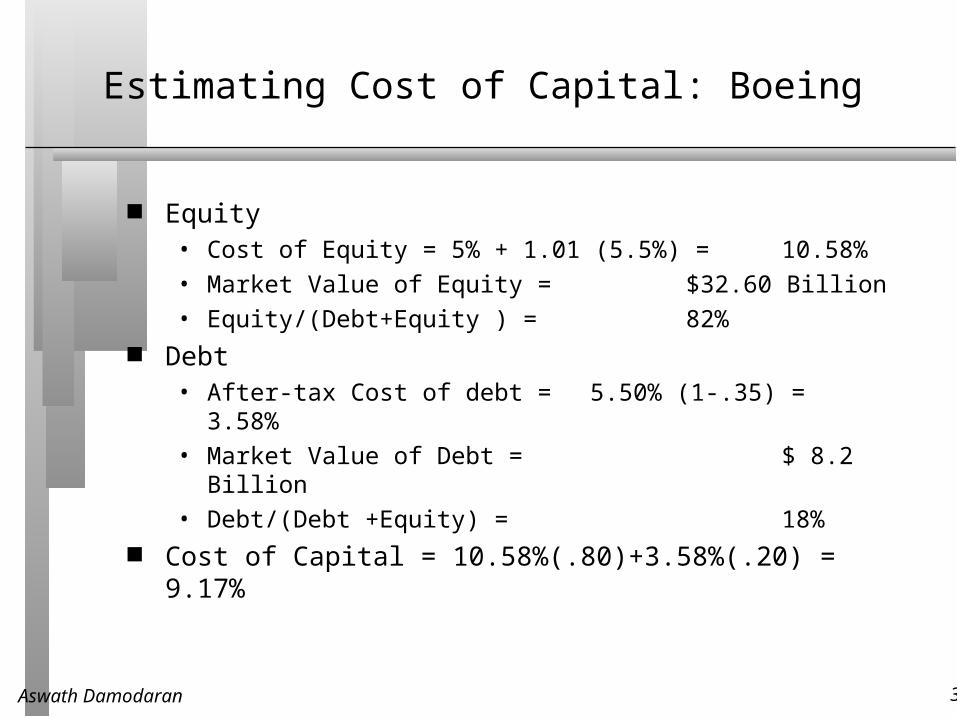
Estimating Cost of Capital: Boeing

Equity• Cost of Equity = 5% + 1.01 (5.5%) = 10.58%

• Market Value of Equity = $32.60 Billion

• Equity/(Debt+Equity ) = 82% Debt

• After-tax Cost of debt = 5.50% (1-.35) = 3.58%

• Market Value of Debt = $ 8.2 Billion

• Debt/(Debt +Equity) = 18% Cost of Capital = 10.58%(.80)+3.58%(.20) = 9.17%

Aswath Damodaran 34

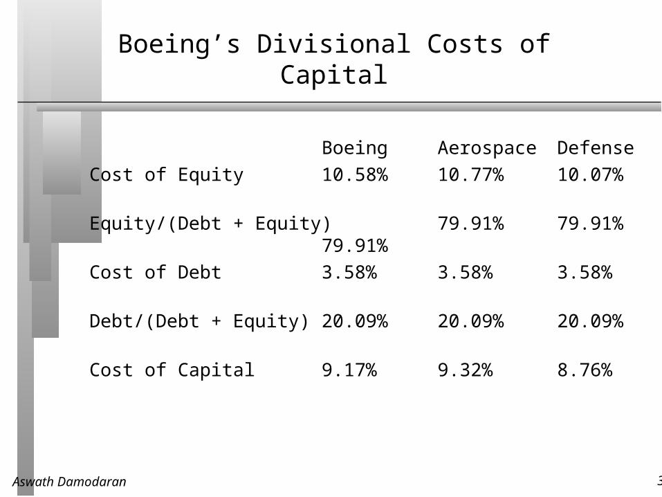
Boeing’s Divisional Costs of Capital

Boeing Aerospace DefenseCost of Equity 10.58% 10.77% 10.07%

Equity/(Debt + Equity) 79.91% 79.91% 79.91%

Cost of Debt 3.58% 3.58% 3.58%

Debt/(Debt + Equity) 20.09% 20.09% 20.09%

Cost of Capital 9.17% 9.32% 8.76%

Aswath Damodaran 35

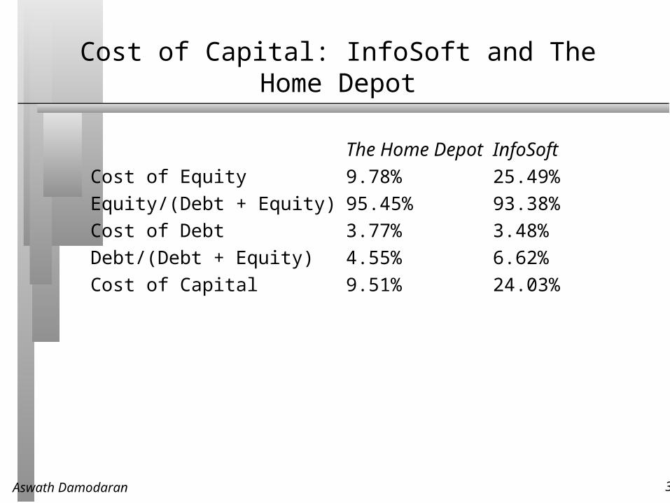
Cost of Capital: InfoSoft and The Home Depot

The Home Depot InfoSoft

Cost of Equity 9.78% 25.49%

Equity/(Debt + Equity) 95.45% 93.38%

Cost of Debt 3.77% 3.48%

Debt/(Debt + Equity) 4.55% 6.62%

Cost of Capital 9.51% 24.03%

Aswath Damodaran 36

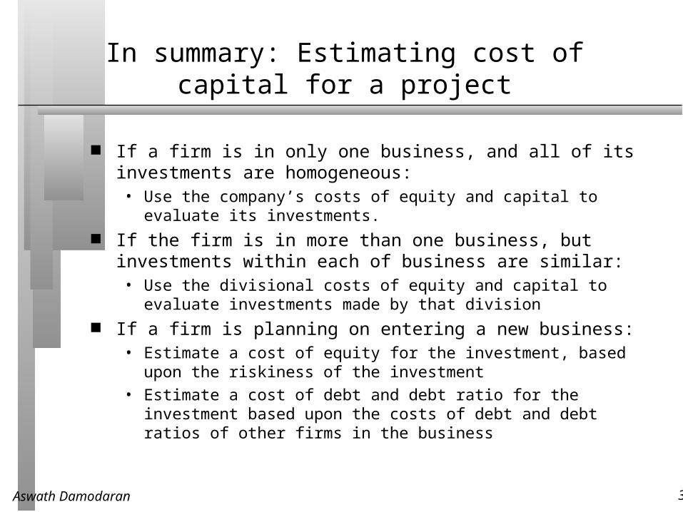
In summary: Estimating cost of capital for a project

If a firm is in only one business, and all of its investments are homogeneous:• Use the company’s costs of equity and capital to evaluate its investments.

If the firm is in more than one business, but investments within each of business are similar:• Use the divisional costs of equity and capital to evaluate investments

made by that division If a firm is planning on entering a new business:

• Estimate a cost of equity for the investment, based upon the riskiness of the investment

• Estimate a cost of debt and debt ratio for the investment based upon the costs of debt and debt ratios of other firms in the business

Aswath Damodaran 37

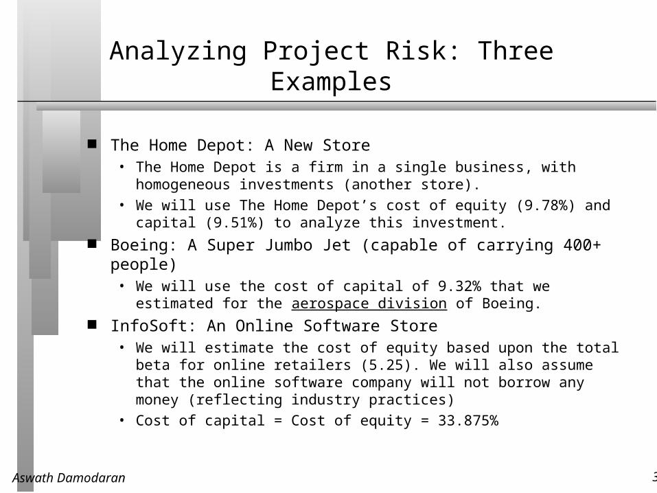
Analyzing Project Risk: Three Examples

The Home Depot: A New Store• The Home Depot is a firm in a single business, with homogeneous

investments (another store).

• We will use The Home Depot’s cost of equity (9.78%) and capital (9.51%) to analyze this investment.

Boeing: A Super Jumbo Jet (capable of carrying 400+ people)• We will use the cost of capital of 9.32% that we estimated for the

aerospace division of Boeing. InfoSoft: An Online Software Store

• We will estimate the cost of equity based upon the total beta for online retailers (5.25). We will also assume that the online software company will not borrow any money (reflecting industry practices)

• Cost of capital = Cost of equity = 33.875%

Aswath Damodaran 38

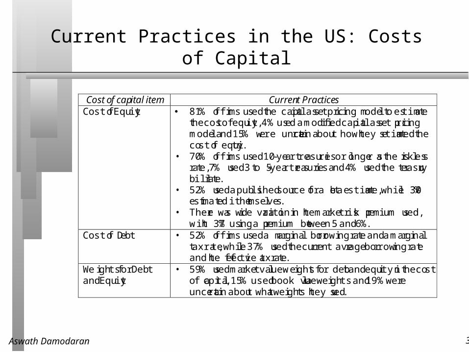
Current Practices in the US: Costs of Capital

Cost of capital item Current PracticesCost of Equity • 81% of fi rms used the capital asset pricing model to estimate

the cost of equity, 4% used a modified capital asset pricingmodel and 15% were uncertain about how they estimated thecost of equtiy.

• 70% of fi rms used 10-year treasuries or longer as the risklessrate, 7% used 3 to 5-year treasuries and 4% used the treasurybill rate.

• 52% used a published source for a beta estimate, while 30%estimated it themselves.

• There was wide variation in the market risk premium used,with 37% using a premium between 5 and 6%.

Cost of Debt • 52% of fi rms used a marginal borrowing rate and a marginaltax rate, while 37% used the current average borrowing rateand the eff ective tax rate.

Weights for Debtand Equity

• 59% used market value weights for debt and equity in the costof capital, 15% used book value weights and 19% wereuncertain about what weights they used.

Aswath Damodaran 39

Choosing a Hurdle Rate

Either the cost of equity or the cost of capital can be used as a hurdle rate, depending upon whether the returns measured are to equity investors or to all claimholders on the firm (capital)

If returns are measured to equity investors, the appropriate hurdle rate is the cost of equity.

If returns are measured to capital (or the firm), the appropriate hurdle rate is the cost of capital.

Aswath Damodaran 40

II. The Estimation Process: Sources of Information/ Estimation

Experience and History: If a firm has invested in similar projects in the past, it can use this experience to estimate revenues and earnings on the project being analyzed.

Market Testing: If the investment is in a new market or business, you can use market testing to get a sense of the size of the market and potential profitability.

Macro economic/ Sector forecasters: There are services that provide forecasts of varying accuracy/ reliability on what they think will happen to the economy or a particular sector.

Market Data: There are some cases where market prices provide information that can be used in forecasts. This is especially the case when you are forecasting interest rates, exchange rates and commodity prices.

Aswath Damodaran 41

Three approaches to estimation

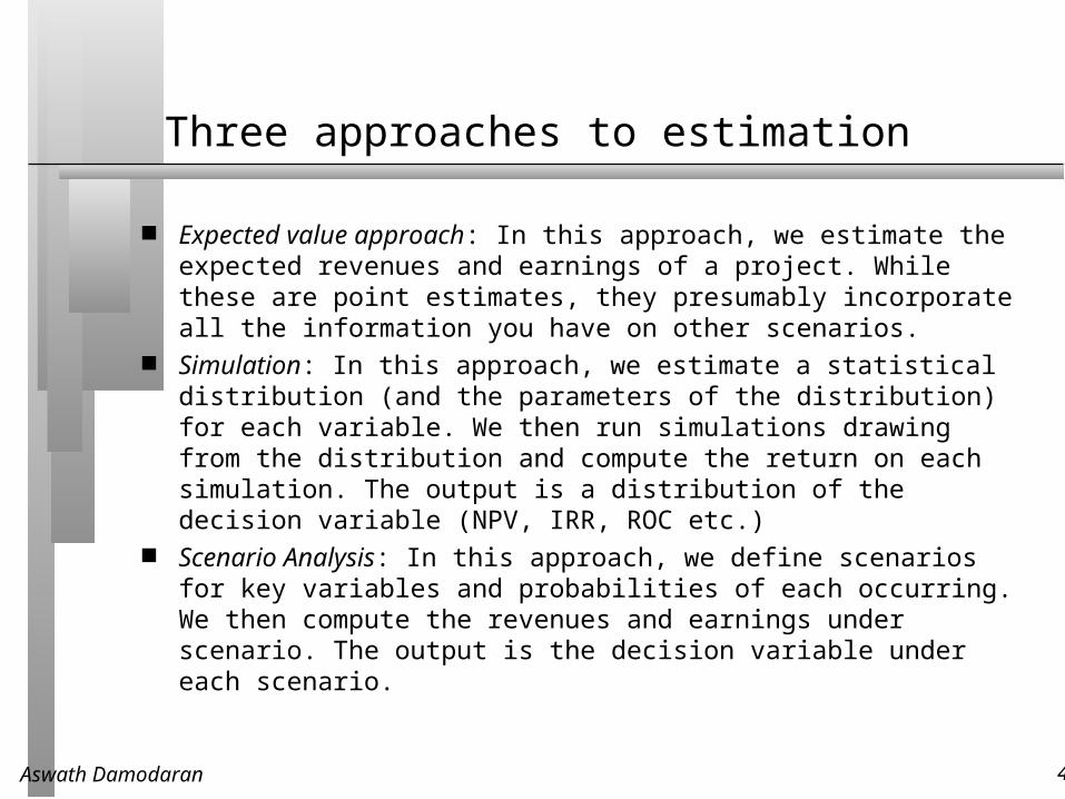
Expected value approach: In this approach, we estimate the expected revenues and earnings of a project. While these are point estimates, they presumably incorporate all the information you have on other scenarios.

Simulation: In this approach, we estimate a statistical distribution (and the parameters of the distribution) for each variable. We then run simulations drawing from the distribution and compute the return on each simulation. The output is a distribution of the decision variable (NPV, IRR, ROC etc.)

Scenario Analysis: In this approach, we define scenarios for key variables and probabilities of each occurring. We then compute the revenues and earnings under scenario. The output is the decision variable under each scenario.

Aswath Damodaran 42

The Home Depot’s New Store: Experience and History

The Home Depot has 700+ stores in existence, at difference stages in their life cycles, yielding valuable information on how much revenue can be expected at each store and expected margins.

At the end of 1999, for instance, each existing store had revenues of $ 44 million, with revenues starting at about $ 40 million in the first year of a store’s life, climbing until year 5 and then declining until year 10.

Aswath Damodaran 43

The Margins at Existing Stores

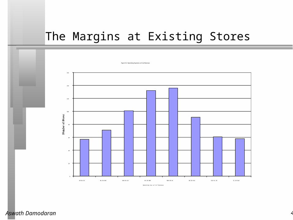
Figure 9.3: Operating Expenses as % of Revenues

0

20

40

60

80

100

120

140

160

88-88.5% 88.5%-89% 89%-89.5% 89.5%-90% 90%-90.5% 90.5%-91% 91%-91.5% 91.5%-92%

Operating Exp as % of Revenues

Aswath Damodaran 44

Projections for The Home Depot’s New Store -Expected Value Analysis

For revenues, we will assume that the new store being considered by the Home Depot will have

expected revenues of $ 40 million in year 1 (which is the approximately the average revenue per store at existing stores after one year in operation)

that these revenues to grow 5% a year

• that our analysis will cover 10 years (since revenues start dropping at existing stores after the 10th year).

For operating margins, we will assume• The operating expenses of the new store will be 90% of the revenues

(based upon the median for existing stores)

Aswath Damodaran 45

The Simulation Alternative

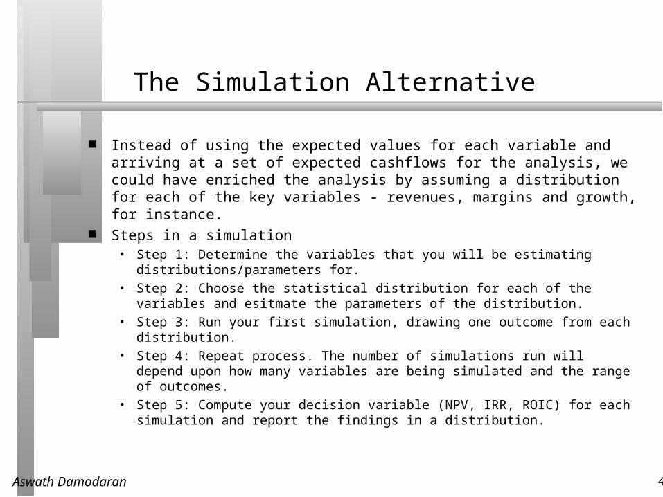
Instead of using the expected values for each variable and arriving at a set of expected cashflows for the analysis, we could have enriched the analysis by assuming a distribution for each of the key variables - revenues, margins and growth, for instance.

Steps in a simulation• Step 1: Determine the variables that you will be estimating distributions/parameters

for.

• Step 2: Choose the statistical distribution for each of the variables and esitmate the parameters of the distribution.

• Step 3: Run your first simulation, drawing one outcome from each distribution.

• Step 4: Repeat process. The number of simulations run will depend upon how many variables are being simulated and the range of outcomes.

• Step 5: Compute your decision variable (NPV, IRR, ROIC) for each simulation and report the findings in a distribution.

Aswath Damodaran 46

What simulations do and what they do not…

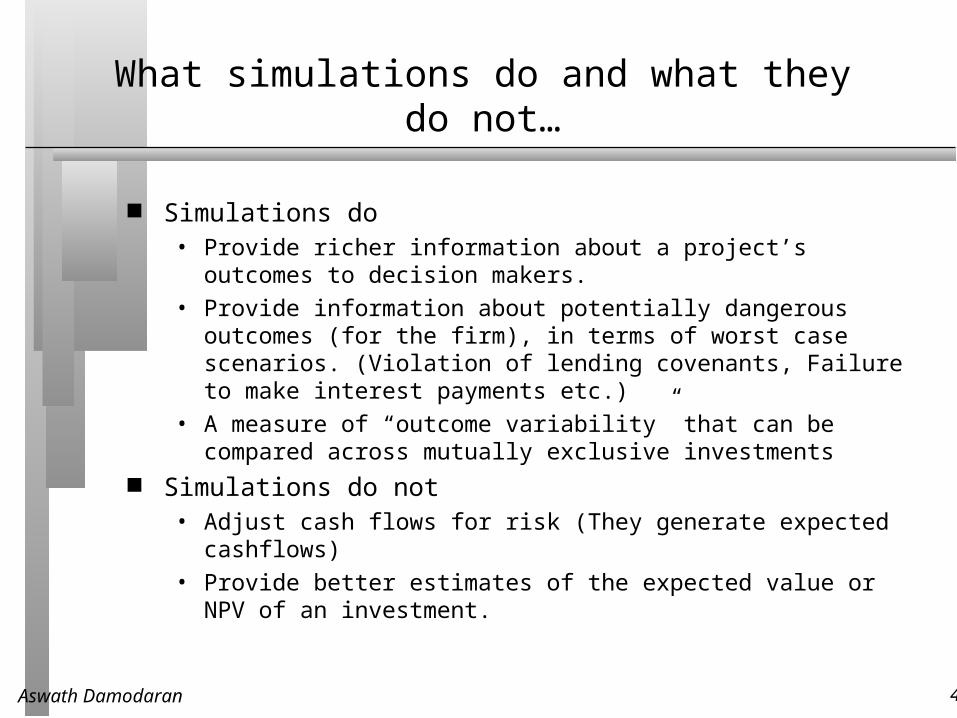
Simulations do• Provide richer information about a project’s outcomes to decision makers.

• Provide information about potentially dangerous outcomes (for the firm), in terms of worst case scenarios. (Violation of lending covenants, Failure to make interest payments etc.)

• A measure of “outcome variability” that can be compared across mutually exclusive investments

Simulations do not• Adjust cash flows for risk (They generate expected cashflows)

• Provide better estimates of the expected value or NPV of an investment.

Aswath Damodaran 47

When simulations make sense and when they do not..

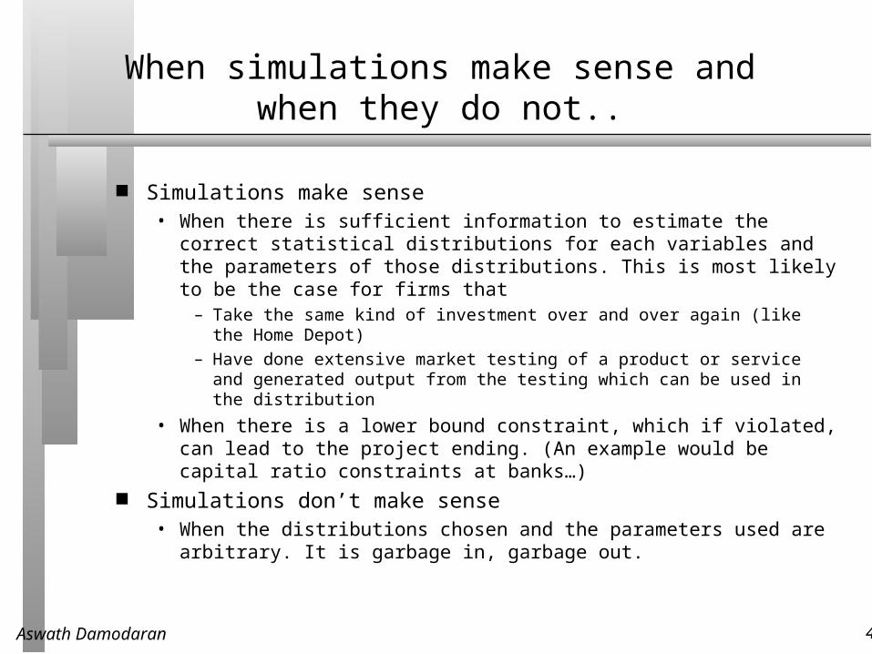
Simulations make sense • When there is sufficient information to estimate the correct statistical

distributions for each variables and the parameters of those distributions. This is most likely to be the case for firms that

– Take the same kind of investment over and over again (like the Home Depot)

– Have done extensive market testing of a product or service and generated output from the testing which can be used in the distribution

• When there is a lower bound constraint, which if violated, can lead to the project ending. (An example would be capital ratio constraints at banks…)

Simulations don’t make sense• When the distributions chosen and the parameters used are arbitrary. It is

garbage in, garbage out.

Aswath Damodaran 48

Scenario Analysis: Boeing Super Jumbo

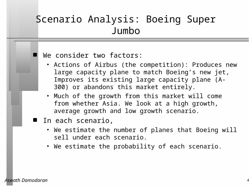
We consider two factors:• Actions of Airbus (the competition): Produces new large capacity plane to

match Boeing’s new jet, Improves its existing large capacity plane (A-300) or abandons this market entirely.

• Much of the growth from this market will come from whether Asia. We look at a high growth, average growth and low growth scenario.

In each scenario,• We estimate the number of planes that Boeing will sell under each

scenario.

• We estimate the probability of each scenario.

Aswath Damodaran 49

Scenario Analysis

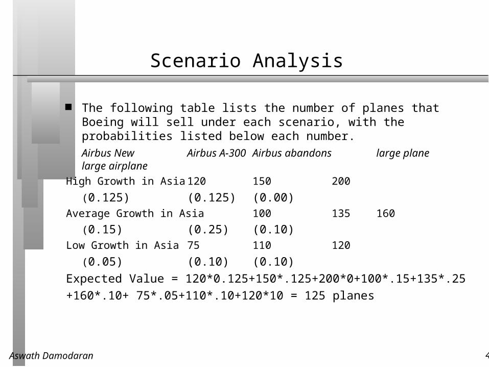
The following table lists the number of planes that Boeing will sell under each scenario, with the probabilities listed below each number.

Airbus New Airbus A-300 Airbus abandons large plane large airplane

High Growth in Asia 120 150 200

(0.125) (0.125) (0.00)Average Growth in Asia 100 135 160

(0.15) (0.25) (0.10)Low Growth in Asia 75 110 120

(0.05) (0.10) (0.10)

Expected Value = 120*0.125+150*.125+200*0+100*.15+135*.25

+160*.10+ 75*.05+110*.10+120*10 = 125 planes

Aswath Damodaran 50

III. Measures of return: Accounting Earnings

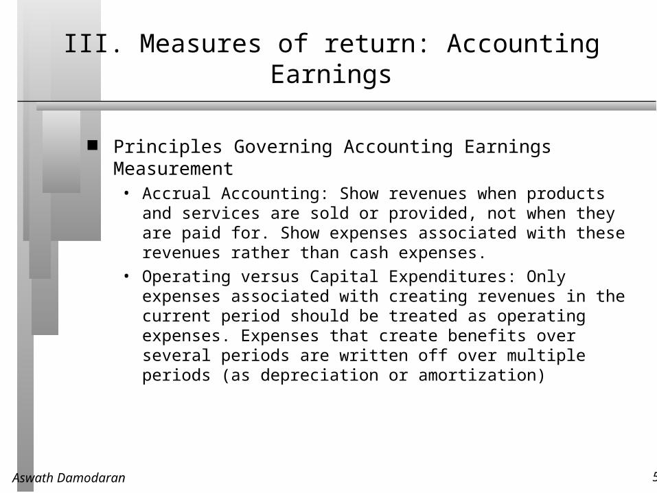
Principles Governing Accounting Earnings Measurement• Accrual Accounting: Show revenues when products and services are sold

or provided, not when they are paid for. Show expenses associated with these revenues rather than cash expenses.

• Operating versus Capital Expenditures: Only expenses associated with creating revenues in the current period should be treated as operating expenses. Expenses that create benefits over several periods are written off over multiple periods (as depreciation or amortization)

Aswath Damodaran 51

From Forecasts to Accounting Earnings

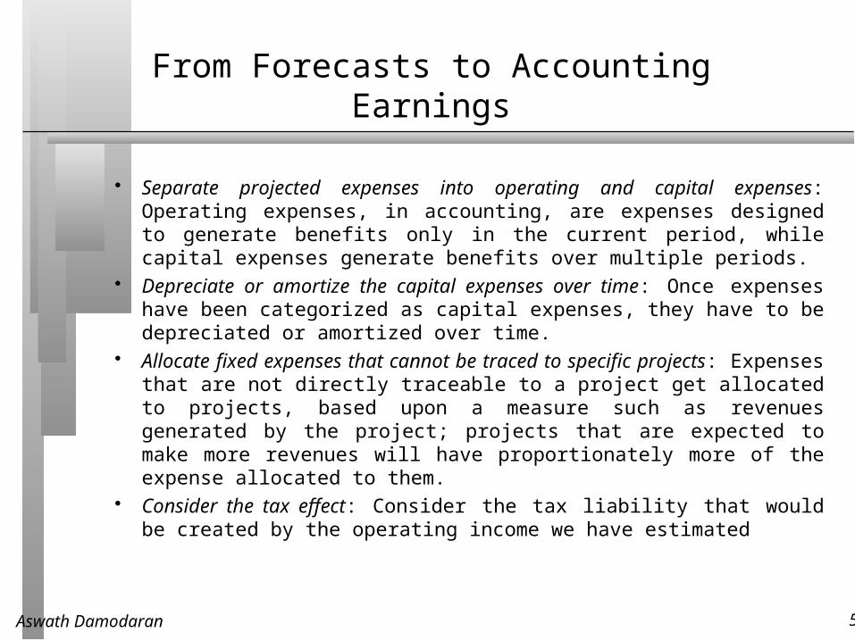
Separate projected expenses into operating and capital expenses: Operating expenses, in accounting, are expenses designed to generate benefits only in the current period, while capital expenses generate benefits over multiple periods.

Depreciate or amortize the capital expenses over time: Once expenses have been categorized as capital expenses, they have to be depreciated or amortized over time.

Allocate fixed expenses that cannot be traced to specific projects: Expenses that are not directly traceable to a project get allocated to projects, based upon a measure such as revenues generated by the project; projects that are expected to make more revenues will have proportionately more of the expense allocated to them.

Consider the tax effect: Consider the tax liability that would be created by the operating income we have estimated

Aswath Damodaran 52

Boeing Super Jumbo Jet: Investment Assumptions

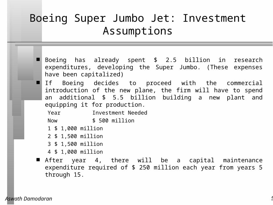
Boeing has already spent $ 2.5 billion in research expenditures, developing the Super Jumbo. (These expenses have been capitalized)

If Boeing decides to proceed with the commercial introduction of the new plane, the firm will have to spend an additional $ 5.5 billion building a new plant and equipping it for production. Year Investment Needed

Now $ 500 million

1 $ 1,000 million

2 $ 1,500 million

3 $ 1,500 million

4 $ 1,000 million After year 4, there will be a capital maintenance expenditure required

of $ 250 million each year from years 5 through 15.

Aswath Damodaran 53

Operating Assumptions

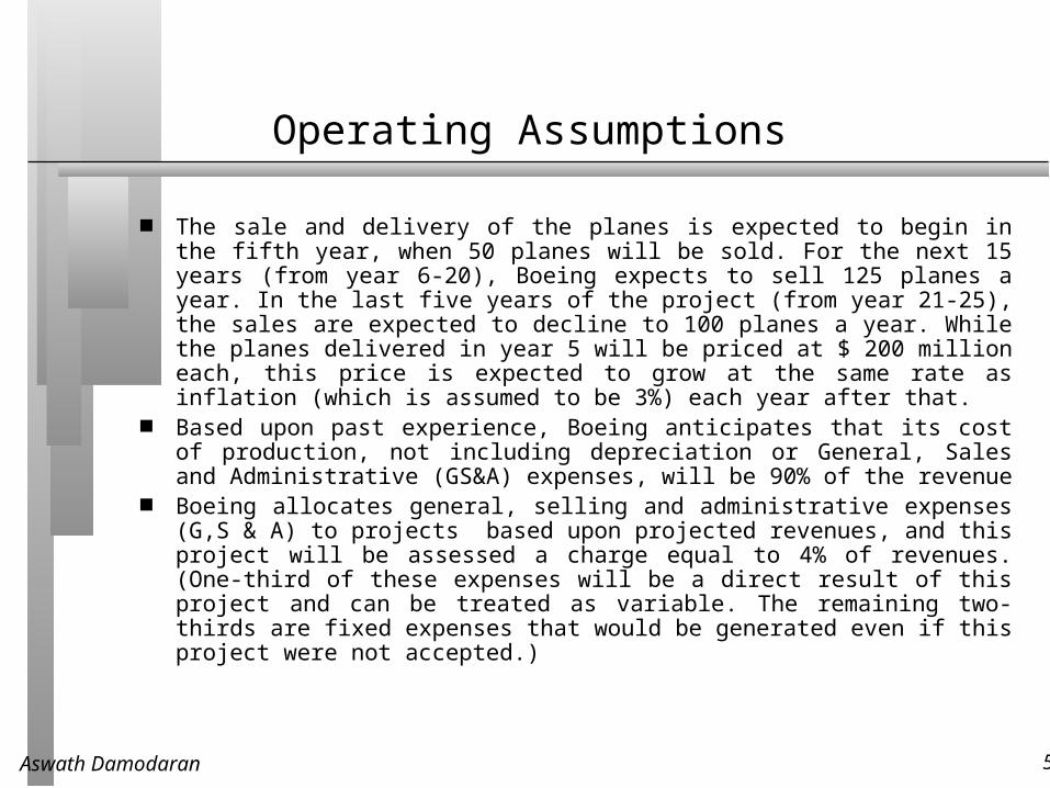
The sale and delivery of the planes is expected to begin in the fifth year, when 50 planes will be sold. For the next 15 years (from year 6-20), Boeing expects to sell 125 planes a year. In the last five years of the project (from year 21-25), the sales are expected to decline to 100 planes a year. While the planes delivered in year 5 will be priced at $ 200 million each, this price is expected to grow at the same rate as inflation (which is assumed to be 3%) each year after that.

Based upon past experience, Boeing anticipates that its cost of production, not including depreciation or General, Sales and Administrative (GS&A) expenses, will be 90% of the revenue

Boeing allocates general, selling and administrative expenses (G,S & A) to projects based upon projected revenues, and this project will be assessed a charge equal to 4% of revenues. (One-third of these expenses will be a direct result of this project and can be treated as variable. The remaining two-thirds are fixed expenses that would be generated even if this project were not accepted.)

Aswath Damodaran 54

Other Assumptions

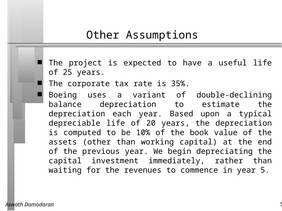
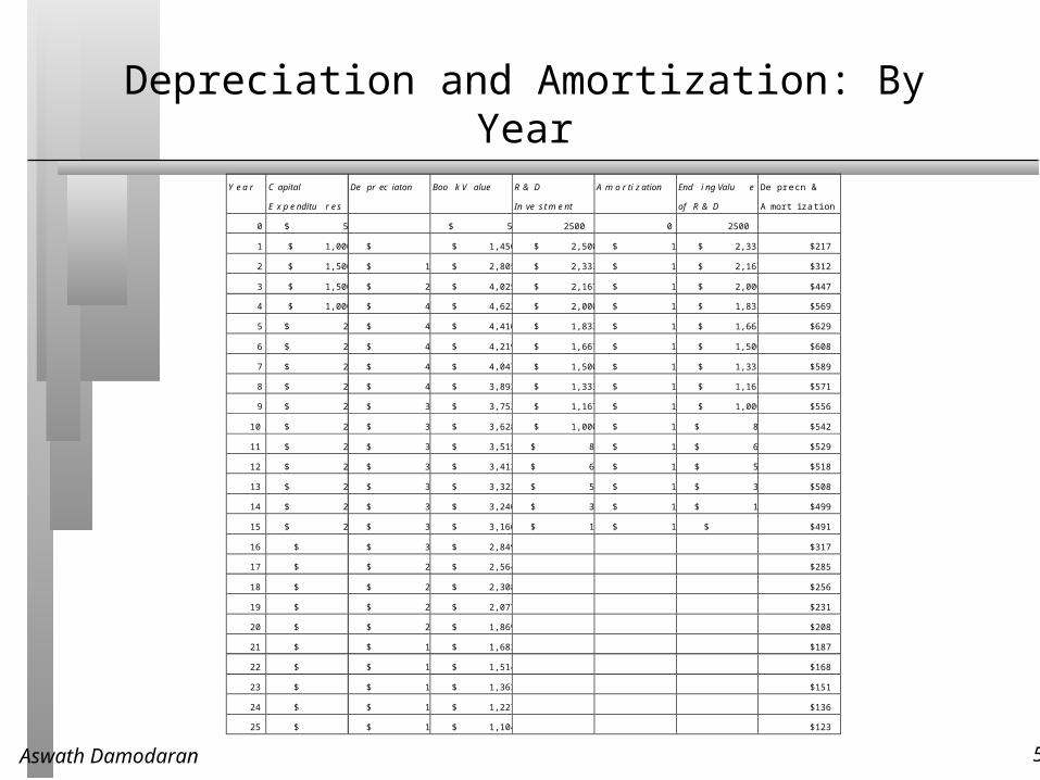
The project is expected to have a useful life of 25 years. The corporate tax rate is 35%. Boeing uses a variant of double-declining balance depreciation to

estimate the depreciation each year. Based upon a typical depreciable life of 20 years, the depreciation is computed to be 10% of the book value of the assets (other than working capital) at the end of the previous year. We begin depreciating the capital investment immediately, rather than waiting for the revenues to commence in year 5.

Aswath Damodaran 55

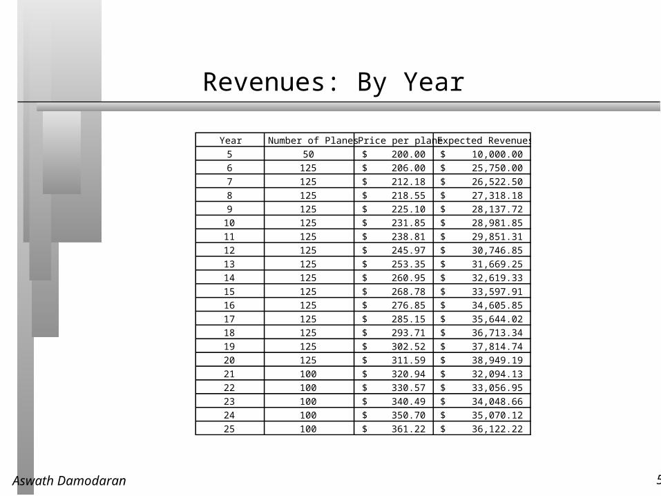
Revenues: By Year

Year Number of Planes Price per plane Expected Revenues5 50 200.00$ 10,000.00$ 6 125 206.00$ 25,750.00$ 7 125 212.18$ 26,522.50$ 8 125 218.55$ 27,318.18$ 9 125 225.10$ 28,137.72$

10 125 231.85$ 28,981.85$ 11 125 238.81$ 29,851.31$ 12 125 245.97$ 30,746.85$ 13 125 253.35$ 31,669.25$ 14 125 260.95$ 32,619.33$ 15 125 268.78$ 33,597.91$ 16 125 276.85$ 34,605.85$ 17 125 285.15$ 35,644.02$ 18 125 293.71$ 36,713.34$ 19 125 302.52$ 37,814.74$ 20 125 311.59$ 38,949.19$ 21 100 320.94$ 32,094.13$ 22 100 330.57$ 33,056.95$ 23 100 340.49$ 34,048.66$ 24 100 350.70$ 35,070.12$ 25 100 361.22$ 36,122.22$

Aswath Damodaran 56

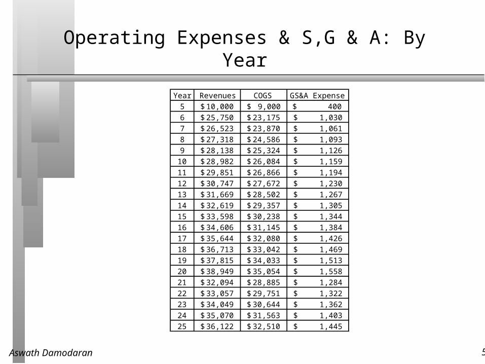
Operating Expenses & S,G & A: By Year

Year Revenues COGS GS&A Expense5 10,000$ 9,000$ 400$ 6 25,750$ 23,175$ 1,030$ 7 26,523$ 23,870$ 1,061$ 8 27,318$ 24,586$ 1,093$ 9 28,138$ 25,324$ 1,126$

10 28,982$ 26,084$ 1,159$ 11 29,851$ 26,866$ 1,194$ 12 30,747$ 27,672$ 1,230$ 13 31,669$ 28,502$ 1,267$ 14 32,619$ 29,357$ 1,305$ 15 33,598$ 30,238$ 1,344$ 16 34,606$ 31,145$ 1,384$ 17 35,644$ 32,080$ 1,426$ 18 36,713$ 33,042$ 1,469$ 19 37,815$ 34,033$ 1,513$ 20 38,949$ 35,054$ 1,558$ 21 32,094$ 28,885$ 1,284$ 22 33,057$ 29,751$ 1,322$ 23 34,049$ 30,644$ 1,362$ 24 35,070$ 31,563$ 1,403$ 25 36,122$ 32,510$ 1,445$

Aswath Damodaran 57

Depreciation and Amortization: By YearY e a r C apital

E x p e nditu r e s

De pr ec iaton Boo k V alue R & D

In ve s t m e nt

A m o r ti z ation End i ng Valu e

of R & D

De pr e cn &

A mort i z a tion

0 $ 500 $ 500 2500 0 2500

1 $ 1,000 $ 50 $ 1,450 $ 2,500 $ 167 $ 2,333 $217

2 $ 1,500 $ 145 $ 2,805 $ 2,333 $ 167 $ 2,167 $312

3 $ 1,500 $ 281 $ 4,025 $ 2,167 $ 167 $ 2,000 $447

4 $ 1,000 $ 402 $ 4,622 $ 2,000 $ 167 $ 1,833 $569

5 $ 250 $ 462 $ 4,410 $ 1,833 $ 167 $ 1,667 $629

6 $ 250 $ 441 $ 4,219 $ 1,667 $ 167 $ 1,500 $608

7 $ 250 $ 422 $ 4,047 $ 1,500 $ 167 $ 1,333 $589

8 $ 250 $ 405 $ 3,892 $ 1,333 $ 167 $ 1,167 $571

9 $ 250 $ 389 $ 3,753 $ 1,167 $ 167 $ 1,000 $556

10 $ 250 $ 375 $ 3,628 $ 1,000 $ 167 $ 833 $542

11 $ 250 $ 363 $ 3,515 $ 833 $ 167 $ 667 $529

12 $ 250 $ 351 $ 3,413 $ 667 $ 167 $ 500 $518

13 $ 250 $ 341 $ 3,322 $ 500 $ 167 $ 333 $508

14 $ 250 $ 332 $ 3,240 $ 333 $ 167 $ 167 $499

15 $ 250 $ 324 $ 3,166 $ 167 $ 167 $ - $491

16 $ - $ 317 $ 2,849 $317

17 $ - $ 285 $ 2,564 $285

18 $ - $ 256 $ 2,308 $256

19 $ - $ 231 $ 2,077 $231

20 $ - $ 208 $ 1,869 $208

21 $ - $ 187 $ 1,683 $187

22 $ - $ 168 $ 1,514 $168

23 $ - $ 151 $ 1,363 $151

24 $ - $ 136 $ 1,227 $136

25 $ - $ 123 $ 1,104 $123

Aswath Damodaran 58

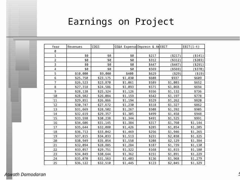
Earnings on Project

Year Revenues COGS GS&A ExpenseDeprecn & AmortizationEBIT EBIT(1-t)01 $0 $0 $0 $217 ($217) ($141)2 $0 $0 $0 $312 ($312) ($203)3 $0 $0 $0 $447 ($447) ($291)4 $0 $0 $0 $569 ($569) ($370)5 $10,000 $9,000 $400 $629 ($29) ($19)6 $25,750 $23,175 $1,030 $608 $937 $6097 $26,523 $23,870 $1,061 $589 $1,003 $6528 $27,318 $24,586 $1,093 $571 $1,068 $6949 $28,138 $25,324 $1,126 $556 $1,132 $736

10 $28,982 $26,084 $1,159 $542 $1,197 $77811 $29,851 $26,866 $1,194 $529 $1,262 $82012 $30,747 $27,672 $1,230 $518 $1,327 $86213 $31,669 $28,502 $1,267 $508 $1,392 $90514 $32,619 $29,357 $1,305 $499 $1,458 $94815 $33,598 $30,238 $1,344 $491 $1,525 $99116 $34,606 $31,145 $1,384 $317 $1,760 $1,14417 $35,644 $32,080 $1,426 $285 $1,854 $1,20518 $36,713 $33,042 $1,469 $256 $1,946 $1,26519 $37,815 $34,033 $1,513 $231 $2,038 $1,32520 $38,949 $35,054 $1,558 $208 $2,129 $1,38421 $32,094 $28,885 $1,284 $187 $1,739 $1,13022 $33,057 $29,751 $1,322 $168 $1,815 $1,18023 $34,049 $30,644 $1,362 $151 $1,891 $1,22924 $35,070 $31,563 $1,403 $136 $1,968 $1,27925 $36,122 $32,510 $1,445 $123 $2,045 $1,329

Aswath Damodaran 59

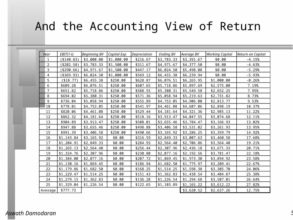
And the Accounting View of Return

Year EBIT(1-t) Beginning BV Capital Exp Depreciation Ending BV Average BV Working Capital Return on Capital1 ($140.83) $3,000.00 $1,000.00 $216.67 $3,783.33 $3,391.67 $0.00 -4.15%2 ($202.58) $3,783.33 $1,500.00 $311.67 $4,971.67 $4,377.50 $0.00 -4.63%3 ($290.66) $4,971.67 $1,500.00 $447.17 $6,024.50 $5,498.08 $0.00 -5.29%4 ($369.93) $6,024.50 $1,000.00 $569.12 $6,455.38 $6,239.94 $0.00 -5.93%5 ($18.77) $6,455.38 $250.00 $628.87 $6,076.51 $6,265.95 $1,000.00 -0.26%6 $609.28 $6,076.51 $250.00 $607.65 $5,718.86 $5,897.69 $2,575.00 7.19%7 $651.82 $5,718.86 $250.00 $588.55 $5,380.31 $5,549.58 $2,652.25 7.95%8 $694.02 $5,380.31 $250.00 $571.36 $5,058.94 $5,219.63 $2,731.82 8.73%9 $736.04 $5,058.94 $250.00 $555.89 $4,753.05 $4,906.00 $2,813.77 9.53%

10 $778.01 $4,753.05 $250.00 $541.97 $4,461.08 $4,607.06 $2,898.19 10.37%11 $820.06 $4,461.08 $250.00 $529.44 $4,181.64 $4,321.36 $2,985.13 11.22%12 $862.32 $4,181.64 $250.00 $518.16 $3,913.47 $4,047.55 $3,074.68 12.11%13 $904.89 $3,913.47 $250.00 $508.01 $3,655.46 $3,784.47 $3,166.93 13.02%14 $947.88 $3,655.46 $250.00 $498.88 $3,406.58 $3,531.02 $3,261.93 13.95%15 $991.39 $3,406.58 $250.00 $490.66 $3,165.92 $3,286.25 $3,359.79 14.92%16 $1,143.84 $3,165.92 $0.00 $316.59 $2,849.33 $3,007.63 $3,460.58 17.68%17 $1,204.91 $2,849.33 $0.00 $284.93 $2,564.40 $2,706.86 $3,564.40 19.21%18 $1,265.13 $2,564.40 $0.00 $256.44 $2,307.96 $2,436.18 $3,671.33 20.71%19 $1,324.76 $2,307.96 $0.00 $230.80 $2,077.16 $2,192.56 $3,781.47 22.18%20 $1,384.00 $2,077.16 $0.00 $207.72 $1,869.45 $1,973.30 $3,894.92 23.58%21 $1,130.16 $1,869.45 $0.00 $186.94 $1,682.50 $1,775.97 $3,209.41 22.67%22 $1,179.86 $1,682.50 $0.00 $168.25 $1,514.25 $1,598.38 $3,305.70 24.06%23 $1,229.47 $1,514.25 $0.00 $151.43 $1,362.83 $1,438.54 $3,404.87 25.38%24 $1,279.15 $1,362.83 $0.00 $136.28 $1,226.54 $1,294.68 $3,507.01 26.64%25 $1,329.04 $1,226.54 $0.00 $122.65 $1,103.89 $1,165.22 $3,612.22 27.82%

Average $777.73 $3,620.52 $2,637.26 12.75%

Aswath Damodaran 60

Would lead use to conclude that...

Invest in the Super Jumbo Jet The return on capital of 12.75% is greater than the cost of capital for aerospace of 9.32%; This would suggest that the project should not be taken.

Aswath Damodaran 61

An extension to existing projects: Return Spreads and EVA

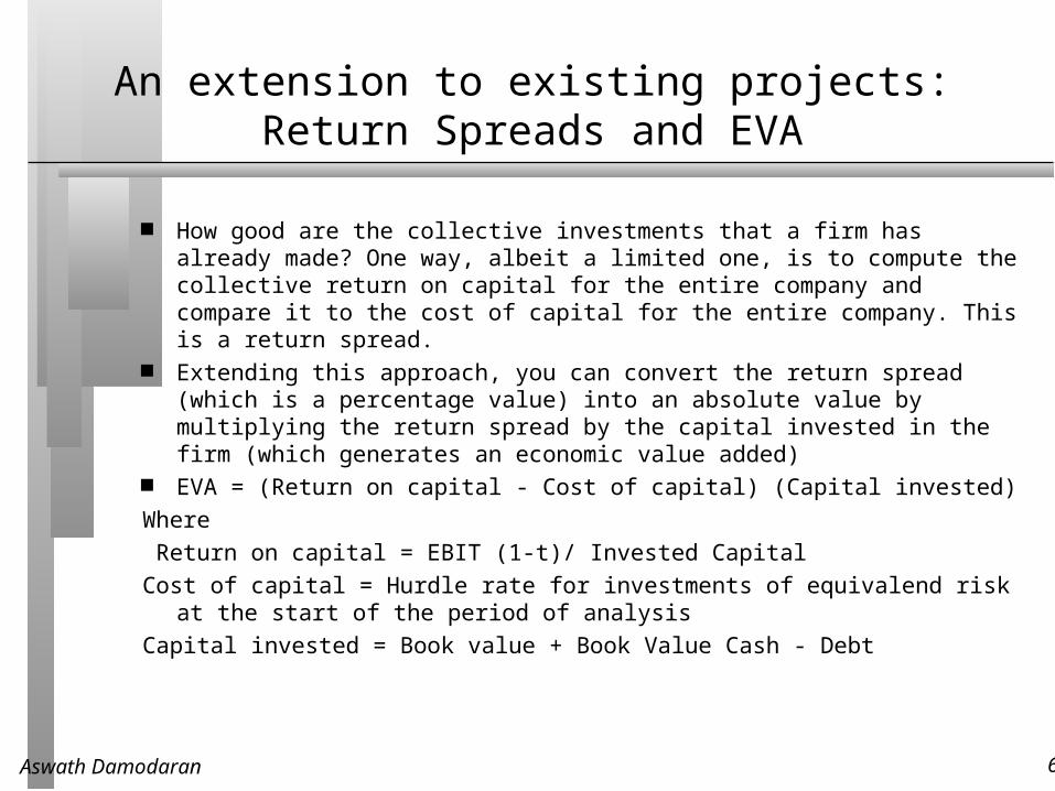
How good are the collective investments that a firm has already made? One way, albeit a limited one, is to compute the collective return on capital for the entire company and compare it to the cost of capital for the entire company. This is a return spread.

Extending this approach, you can convert the return spread (which is a percentage value) into an absolute value by multiplying the return spread by the capital invested in the firm (which generates an economic value added)

EVA = (Return on capital - Cost of capital) (Capital invested)

Where

Return on capital = EBIT (1-t)/ Invested Capital

Cost of capital = Hurdle rate for investments of equivalend risk at the start of the period of analysis

Capital invested = Book value + Book Value Cash - Debt

Aswath Damodaran 62

EVAs and project quality

The EVA for a project is good measure of project quality when• Project earnings closely resemble cashflows.

• Project earnings are measured consistently and the annual cashflows are fairly uniform over time.

• The firm using its is a mature firm with most of its assets already in place with little or no investment needed for long term grosth.

The EVA for a project is a poor measures of project quality when• Project earnings are being manipulated by questionable accounting

practices.

• Project are volatile and change over time.

• The firm is a growth firm with most of its value from growth assets.

Aswath Damodaran 63

From Project to Firm Return on Capital

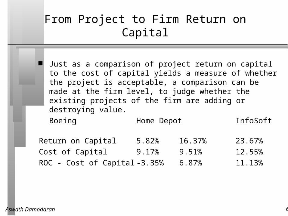
Just as a comparison of project return on capital to the cost of capital yields a measure of whether the project is acceptable, a comparison can be made at the firm level, to judge whether the existing projects of the firm are adding or destroying value.

Boeing Home Depot InfoSoft

Return on Capital 5.82% 16.37% 23.67%

Cost of Capital 9.17% 9.51% 12.55%

ROC - Cost of Capital -3.35% 6.87% 11.13%

Aswath Damodaran 64

IV. From Earnings to Cash Flows

To get from accounting earnings to cash flows:• you have to add back non-cash expenses (like depreciation and

amortization)

• you have to subtract out cash outflows which are not expensed (such as capital expenditures)

• you have to make accrual revenues and expenses into cash revenues and expenses (by considering changes in working capital).

For the Boeing Super Jumbo, we will assume that• The depreciation used for operating expense purposes is also the tax

depreciation.

• Working capital will be 10% of revenues, and the investment has to be made at the beginning of each year.

Aswath Damodaran 65

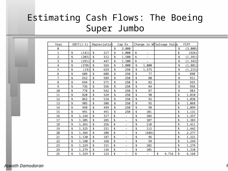
Estimating Cash Flows: The Boeing Super Jumbo

Year EBIT(1-t) Depreciation Cap Ex Change in WC Salvage Value FCFF0 3,000$ (3,000)$ 1 (141)$ 217$ 1,000$ -$ (924)$ 2 (203)$ 312$ 1,500$ -$ (1,391)$ 3 (291)$ 447$ 1,500$ -$ (1,343)$ 4 (370)$ 569$ 1,000$ 1,000$ (1,801)$ 5 (19)$ 629$ 250$ 1,575$ (1,215)$ 6 609$ 608$ 250$ 77$ 890$ 7 652$ 589$ 250$ 80$ 911$ 8 694$ 571$ 250$ 82$ 933$ 9 736$ 556$ 250$ 84$ 958$

10 778$ 542$ 250$ 87$ 983$ 11 820$ 529$ 250$ 90$ 1,010$ 12 862$ 518$ 250$ 92$ 1,038$ 13 905$ 508$ 250$ 95$ 1,068$ 14 948$ 499$ 250$ 98$ 1,099$ 15 991$ 491$ 250$ 101$ 1,131$ 16 1,144$ 317$ -$ 104$ 1,357$ 17 1,205$ 285$ -$ 107$ 1,383$ 18 1,265$ 256$ -$ 110$ 1,411$ 19 1,325$ 231$ -$ 113$ 1,442$ 20 1,384$ 208$ -$ (686)$ 2,277$ 21 1,130$ 187$ -$ 96$ 1,221$ 22 1,180$ 168$ -$ 99$ 1,249$ 23 1,229$ 151$ -$ 102$ 1,279$ 24 1,279$ 136$ -$ 105$ 1,310$ 25 1,329$ 123$ -$ -$ 4,716$ 6,168$

Aswath Damodaran 66

The Depreciation Tax Benefit

While depreciation reduces taxable income and taxes, it does not reduce the cash flows.

The benefit of depreciation is therefore the tax benefit. In general, the tax benefit from depreciation can be written as:

Tax Benefit = Depreciation * Tax Rate For example, in year 2, the tax benefit from depreciation to Boeing from

this project can be written as:

Tax Benefit in year 2 = $ 217 million (.35) = $ 76 million Proposition 1: The tax benefit from depreciation and other non-cash

charges is greater, the higher your tax rate. Proposition 2: Non-cash charges that are not tax deductible (such as

amortization of goodwill) and thus provide no tax benefits have no effect on cash flows.

Aswath Damodaran 67

The Capital Expenditures Effect

Capital expenditures are not treated as accounting expenses but they do cause cash outflows.

Capital expenditures can generally be categorized into two groups• New (or Growth) capital expenditures are capital expenditures designed

to create new assets and future growth

• Maintenance capital expenditures refer to capital expenditures designed to keep existing assets.

Both initial and maintenance capital expenditures reduce cash flows The need for maintenance capital expenditures will increase with the

life of the project. In other words, a 25-year project will require more maintenance capital expenditures than a 2-year asset.

Aswath Damodaran 68

The Working Capital Effect

Intuitively, money invested in inventory or in accounts receivable cannot be used elsewhere. It, thus, represents a drain on cash flows.

To the degree that some of these investments can be financed using suppliers credit (accounts payable) the cash flow drain is reduced.

Assets that earn a fair market return should not be counted as part of working capital for cash flow purposes. Since cash is usually invested to earn a fair market return in marketable securities, it should generally not be considered as part of working capital.

Investments in working capital are thus cash outflows• Any increase in working capital reduces cash flows in that year• Any decrease in working capital increases cash flows in that year

To provide closure, working capital investments need to be salvaged at the end of the project life.

Aswath Damodaran 69

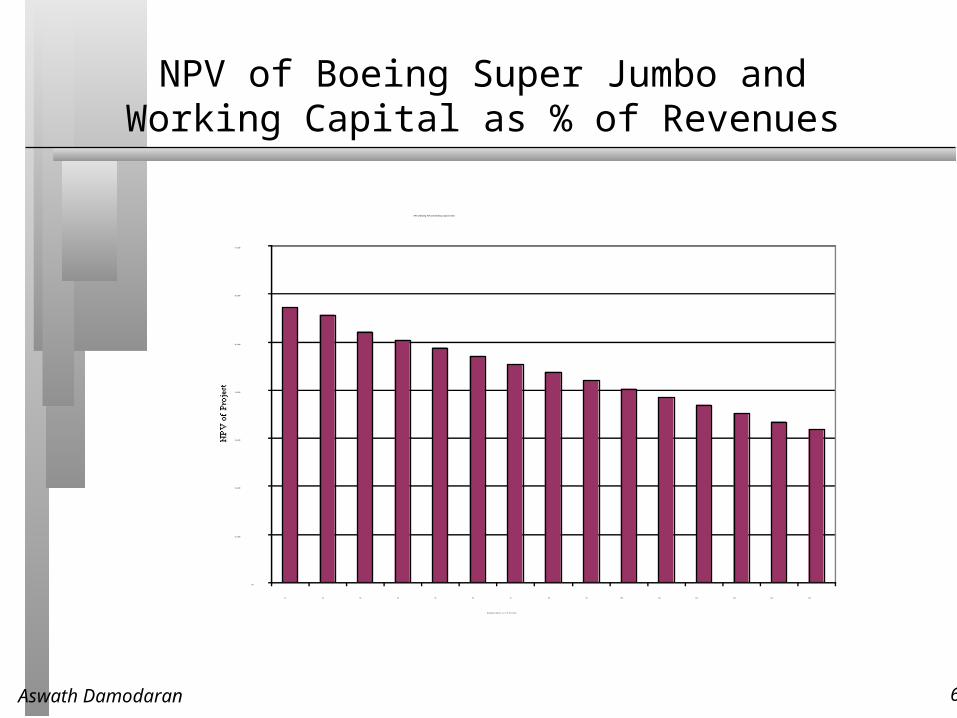
NPV of Boeing Super Jumbo and Working Capital as % of Revenues

NPV of Boeing 747 and Working Capital needs

$0

$1,000

$2,000

$3,000

$4,000

$5,000

$6,000

$7,000

1% 2% 3% 4% 5% 6% 7% 8% 9% 10% 11% 12% 13% 14% 15%

Working Capital as % of Revenues

Aswath Damodaran 70

V. From Cash Flows to Incremental Cash Flows

The incremental cash flows of a project are the difference between the cash flows that the firm would have had, if it accepts the investment, and the cash flows that the firm would have had, if it does not accept the investment.

The Key Questions to determine whether a cash flow is incremental:• What will happen to this cash flow item if I accept the investment?

• What will happen to this cash flow item if I do not accept the investment? If the cash flow will occur whether you take this investment or reject

it, it is not an incremental cash flow.

Aswath Damodaran 71

Sunk Costs

Any expenditure that has already been incurred, and cannot be recovered (even if a project is rejected) is called a sunk cost

When analyzing a project, sunk costs should not be considered since they are incremental

By this definition, market testing expenses and R&D expenses are both likely to be sunk costs before the projects that are based upon them are analyzed. If sunk costs are not considered in project analysis, how can a firm ensure that these costs are covered?

Aswath Damodaran 72

Allocated Costs

Firms allocate costs to individual projects from a centralized pool (such as general and administrative expenses) based upon some characteristic of the project (sales is a common choice)

For large firms, these allocated costs can result in the rejection of projects

To the degree that these costs are not incremental (and would exist anyway), this makes the firm worse off.• Thus, it is only the incremental component of allocated costs that should

show up in project analysis. How, looking at these pooled expenses, do we know how much of the

costs are fixed and how much are variable?

Aswath Damodaran 73

Boeing: Super Jumbo Jet

The $2.5 billion already expended on the jet is a sunk cost, as is the amortization related that expense. (Boeing has spent the first, and it is entitled to the latter even if the investment is rejected)

Two-thirds of the S,G&A expenses are fixed expenses and would exist even if this project is not accepted.

Aswath Damodaran 74

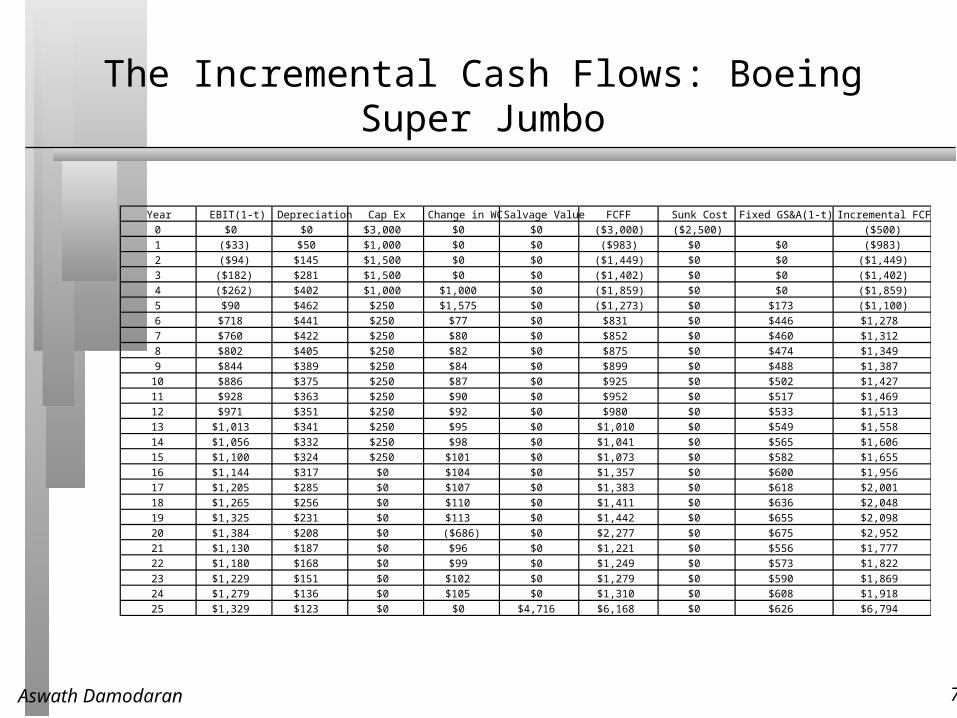
The Incremental Cash Flows: Boeing Super Jumbo

Aswath Damodaran 75

VI. To Time-Weighted Cash Flows

Incremental cash flows in the earlier years are worth more than incremental cash flows in later years.

In fact, cash flows across time cannot be added up. They have to be brought to the same point in time before aggregation.

This process of moving cash flows through time is• discounting, when future cash flows are brought to the present

• compounding, when present cash flows are taken to the future The discount rate is the mechanism that determines how cash flows

across time will be weighted.

Aswath Damodaran 76

Discounted cash flow measures of return

Net Present Value (NPV): The net present value is the sum of the present values of all cash flows from the project (including initial investment).NPV = Sum of the present values of all cash flows on the project, including

the initial investment, with the cash flows being discounted at the appropriate hurdle rate (cost of capital, if cash flow is cash flow to the firm, and cost of equity, if cash flow is to equity investors)

• Decision Rule: Accept if NPV > 0 Internal Rate of Return (IRR): The internal rate of return is the

discount rate that sets the net present value equal to zero. It is the percentage rate of return, based upon incremental time-weighted cash flows.• Decision Rule: Accept if IRR > hurdle rate

Aswath Damodaran 77

Closure on Cash Flows

In a project with a finite and short life, you would need to compute a salvage value, which is the expected proceeds from selling all of the investment in the project at the end of the project life. It is usually set equal to book value of fixed assets and working capital

In a project with an infinite or very long life, we compute cash flows for a reasonable period, and then compute a terminal value for this project, which is the present value of all cash flows that occur after the estimation period ends..

Aswath Damodaran 78

Salvage Value on Boeing Super Jumbo

We will assume that the salvage value for this investment at the end of year 25 will be the book value of the investment.

Book value of capital investments at end of year 25 = $1,104 million

Book value of working capital investments: yr 25 = $3,612 million

Salvage Value at end of year 25 = $4,716 million

Aswath Damodaran 79

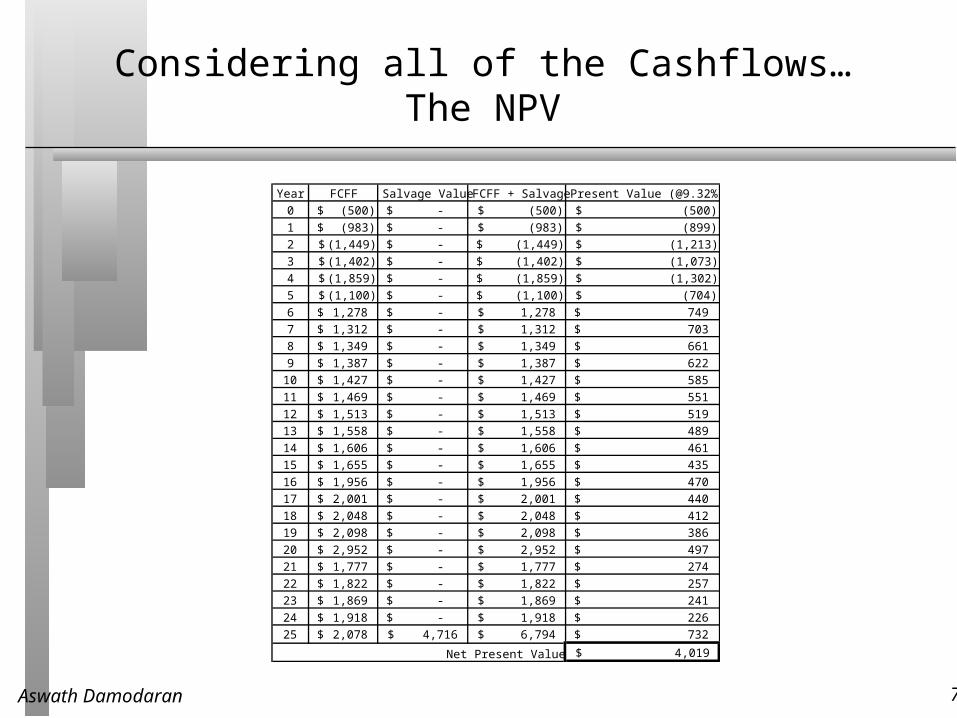
Considering all of the Cashflows… The NPV

Year FCFF Salvage Value FCFF + Salvage Present Value (@9.32%)0 (500)$ -$ (500)$ (500)$ 1 (983)$ -$ (983)$ (899)$ 2 (1,449)$ -$ (1,449)$ (1,213)$ 3 (1,402)$ -$ (1,402)$ (1,073)$ 4 (1,859)$ -$ (1,859)$ (1,302)$ 5 (1,100)$ -$ (1,100)$ (704)$ 6 1,278$ -$ 1,278$ 749$ 7 1,312$ -$ 1,312$ 703$ 8 1,349$ -$ 1,349$ 661$ 9 1,387$ -$ 1,387$ 622$

10 1,427$ -$ 1,427$ 585$ 11 1,469$ -$ 1,469$ 551$ 12 1,513$ -$ 1,513$ 519$ 13 1,558$ -$ 1,558$ 489$ 14 1,606$ -$ 1,606$ 461$ 15 1,655$ -$ 1,655$ 435$ 16 1,956$ -$ 1,956$ 470$ 17 2,001$ -$ 2,001$ 440$ 18 2,048$ -$ 2,048$ 412$ 19 2,098$ -$ 2,098$ 386$ 20 2,952$ -$ 2,952$ 497$ 21 1,777$ -$ 1,777$ 274$ 22 1,822$ -$ 1,822$ 257$ 23 1,869$ -$ 1,869$ 241$ 24 1,918$ -$ 1,918$ 226$ 25 2,078$ 4,716$ 6,794$ 732$

4,019$ Net Present Value =

Aswath Damodaran 80

Which makes the argument that..

The project should be accepted. The positive net present value suggests that the project will add value to the firm, and earn a return in excess of the cost of capital.

By taking the project, Boeing will increase its value as a firm by $4,019 million.

Aswath Damodaran 81

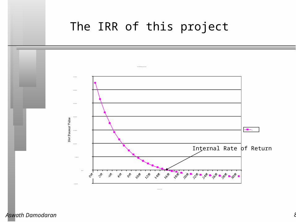
The IRR of this project

NPV Profile: Boeing Super Jumbo

($5,000.00)

$0.00

$5,000.00

$10,000.00

$15,000.00

$20,000.00

$25,000.00

$30,000.00

$35,000.00

Discount Rate

NPV

Internal Rate of Return

Aswath Damodaran 82

The IRR suggests..

The project is a good one. Using time-weighted, incremental cash flows, this project provides a return of 14.88%. This is greater than the cost of capital of 9.32%.

The IRR and the NPV will yield similar results most of the time, though there are differences between the two approaches that may cause project rankings to vary depending upon the approach used.

Aswath Damodaran 83

An IRR-based Approach to analyzing existing investments - CFROI

The CFROI is the internal rate of return that you generate by looking collectively at the investment in all of your assets and the cashflows you expect to generate from them. CFROI is usually done in real terms and should generally be compared to a real cost of capital.

In terms of inputs, CFROI is usually computed using the following:• Gross investment in plant and equipment, which is obtained by adding

back accumulated depreciation to net plant and equipment, is used as the equivalent of the initial investment.

• The annual cashflow is computed by adding back depreciation to after-tax operating income.

• The life of the asset, at the time of the original purchase, is used as the life of the assets

Aswath Damodaran 84

Equity Analysis: The Parallels

The investment analysis can be done entirely in equity terms, as well. The returns, cashflows and hurdle rates will all be defined from the perspective of equity investors.

If using accounting returns,• Return will be Return on Equity (ROE) = Net Income/BV of Equity

• ROE has to be greater than cost of equity If using discounted cashflow models,

• Cashflows will be cashflows after debt payments to equity investors

• Hurdle rate will be cost of equity

Aswath Damodaran 85

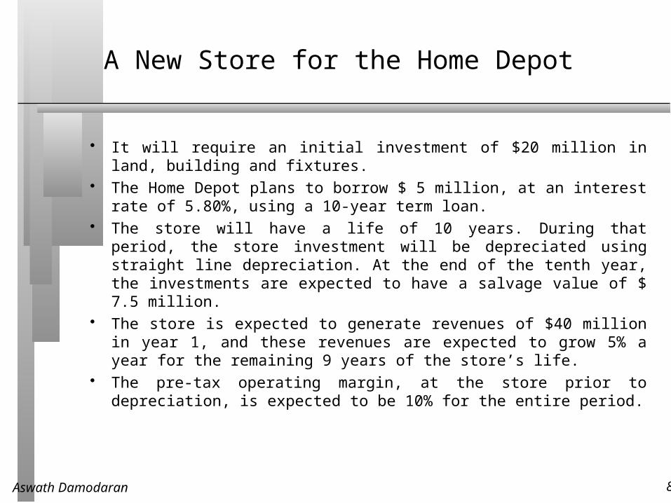
A New Store for the Home Depot

It will require an initial investment of $20 million in land, building and fixtures.

The Home Depot plans to borrow $ 5 million, at an interest rate of 5.80%, using a 10-year term loan.

The store will have a life of 10 years. During that period, the store investment will be depreciated using straight line depreciation. At the end of the tenth year, the investments are expected to have a salvage value of $ 7.5 million.

The store is expected to generate revenues of $40 million in year 1, and these revenues are expected to grow 5% a year for the remaining 9 years of the store’s life.

The pre-tax operating margin, at the store prior to depreciation, is expected to be 10% for the entire period.

Aswath Damodaran 86

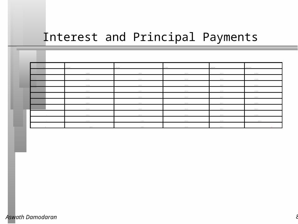
Interest and Principal Payments

Year Outstanding debt Interest Expense Total Payment Principal Repaid Remaining Principal

1 $5,000,000.00 $290,000.00 $672,917.36 $382,917.36 $4,617,082.64

2 $4,617,082.64 $267,790.79 $672,917.36 $405,126.57 $4,211,956.08

3 $4,211,956.08 $244,293.45 $672,917.36 $428,623.91 $3,783,332.17

4 $3,783,332.17 $219,433.27 $672,917.36 $453,484.09 $3,329,848.08

5 $3,329,848.08 $193,131.19 $672,917.36 $479,786.17 $2,850,061.91

6 $2,850,061.91 $165,303.59 $672,917.36 $507,613.77 $2,342,448.14

7 $2,342,448.14 $135,861.99 $672,917.36 $537,055.37 $1,805,392.77

8 $1,805,392.77 $104,712.78 $672,917.36 $568,204.58 $1,237,188.19

9 $1,237,188.19 $71,756.92 $672,917.36 $601,160.44 $636,027.75

10 $636,027.75 $36,889.61 $672,917.36 $636,027.75 $0.00

Aswath Damodaran 87

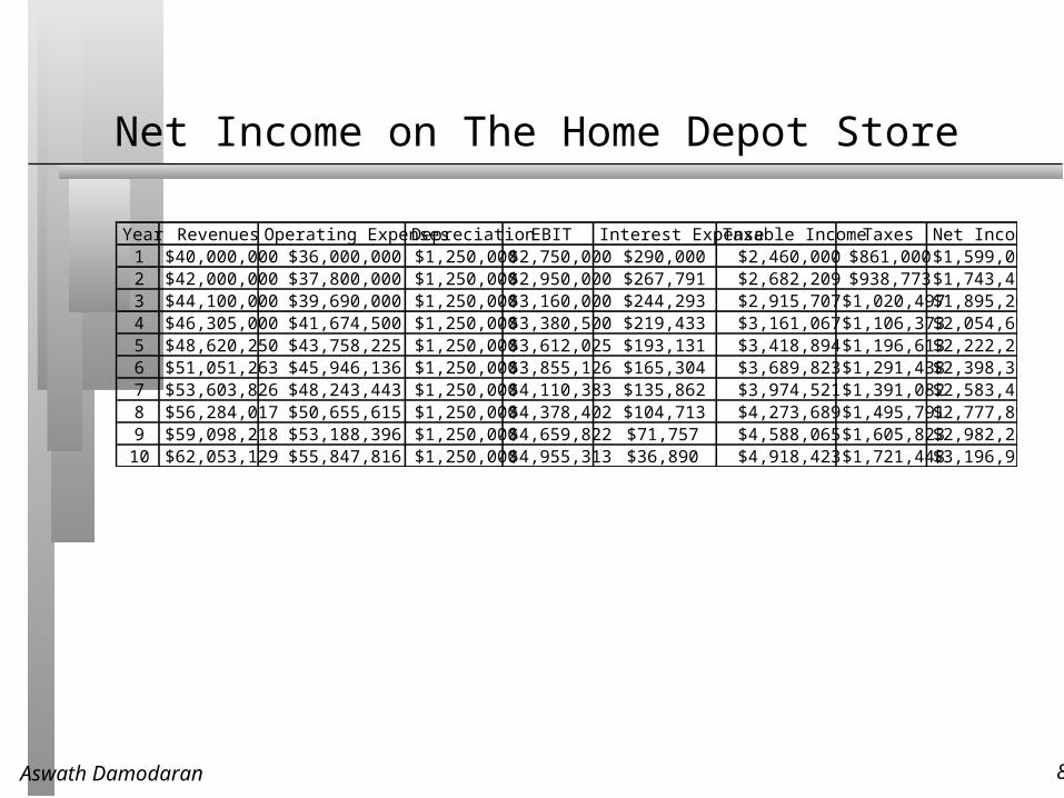
Net Income on The Home Depot Store

Year Revenues Operating Expenses Depreciation EBIT Interest Expense Taxable Income Taxes Net Income1 $40,000,000 $36,000,000 $1,250,000 $2,750,000 $290,000 $2,460,000 $861,000 $1,599,0002 $42,000,000 $37,800,000 $1,250,000 $2,950,000 $267,791 $2,682,209 $938,773 $1,743,4363 $44,100,000 $39,690,000 $1,250,000 $3,160,000 $244,293 $2,915,707 $1,020,497 $1,895,2094 $46,305,000 $41,674,500 $1,250,000 $3,380,500 $219,433 $3,161,067 $1,106,373 $2,054,6935 $48,620,250 $43,758,225 $1,250,000 $3,612,025 $193,131 $3,418,894 $1,196,613 $2,222,2816 $51,051,263 $45,946,136 $1,250,000 $3,855,126 $165,304 $3,689,823 $1,291,438 $2,398,3857 $53,603,826 $48,243,443 $1,250,000 $4,110,383 $135,862 $3,974,521 $1,391,082 $2,583,4388 $56,284,017 $50,655,615 $1,250,000 $4,378,402 $104,713 $4,273,689 $1,495,791 $2,777,8989 $59,098,218 $53,188,396 $1,250,000 $4,659,822 $71,757 $4,588,065 $1,605,823 $2,982,242

10 $62,053,129 $55,847,816 $1,250,000 $4,955,313 $36,890 $4,918,423 $1,721,448 $3,196,975

Aswath Damodaran 88

The Hurdle Rate

The analysis is done in equity terms. Thus, the hurdle rate has to be a cost of equity

The cost of equity for the Home Depot is 9.78%. Since the Home Depot’s investments are assumed to be homogeneous, the cost of equity for this project is also assumed to be 9.78%.

Aswath Damodaran 89

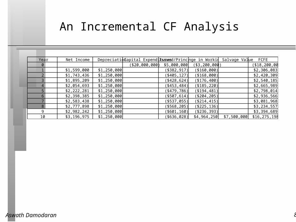
An Incremental CF Analysis

Year Net Income Depreciation Capital ExpendituresDebt Issued/Principal RepaymentChange in Working CapitalSalvage Value FCFE0 ($20,000,000) $5,000,000 ($3,200,000) ($18,200,000)1 $1,599,000 $1,250,000 ($382,917) ($160,000) $2,306,0832 $1,743,436 $1,250,000 ($405,127) ($168,000) $2,420,3093 $1,895,209 $1,250,000 ($428,624) ($176,400) $2,540,1854 $2,054,693 $1,250,000 ($453,484) ($185,220) $2,665,9895 $2,222,281 $1,250,000 ($479,786) ($194,481) $2,798,0146 $2,398,385 $1,250,000 ($507,614) ($204,205) $2,936,5667 $2,583,438 $1,250,000 ($537,055) ($214,415) $3,081,9688 $2,777,898 $1,250,000 ($568,205) ($225,136) $3,234,5579 $2,982,242 $1,250,000 ($601,160) ($236,393) $3,394,689

10 $3,196,975 $1,250,000 ($636,028) $4,964,250 $7,500,000 $16,275,198

Aswath Damodaran 90

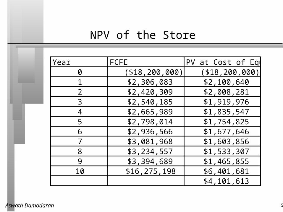
NPV of the Store

Year FCFE PV at Cost of Equity0 ($18,200,000) ($18,200,000)1 $2,306,083 $2,100,6402 $2,420,309 $2,008,2813 $2,540,185 $1,919,9764 $2,665,989 $1,835,5475 $2,798,014 $1,754,8256 $2,936,566 $1,677,6467 $3,081,968 $1,603,8568 $3,234,557 $1,533,3079 $3,394,689 $1,465,855

10 $16,275,198 $6,401,681$4,101,613

Aswath Damodaran 91

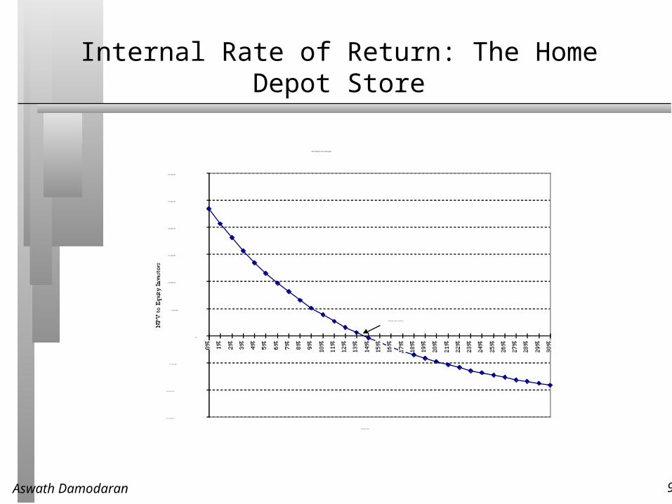
Internal Rate of Return: The Home Depot Store

NPV Profile for The Home Depot

($15,000,000)

($10,000,000)

($5,000,000)

$0

$5,000,000

$10,000,000

$15,000,000

$20,000,000

$25,000,000

$30,000,000

Discount Rate

Internal Rate of Return

Aswath Damodaran 92

The ‘‘Consistency Rule” for Cash Flows

The cash flows on a project and the discount rate used should be defined in the same terms. • If cash flows are in one currency, the discount rate has to be a dollar

(baht) discount rate

• If the cash flows are nominal (real), the discount rate has to be nominal (real).

If consistency is maintained, the project conclusions should be identical, no matter what cash flows are used.

Aswath Damodaran 93

The Home Depot: A New Store in Chile

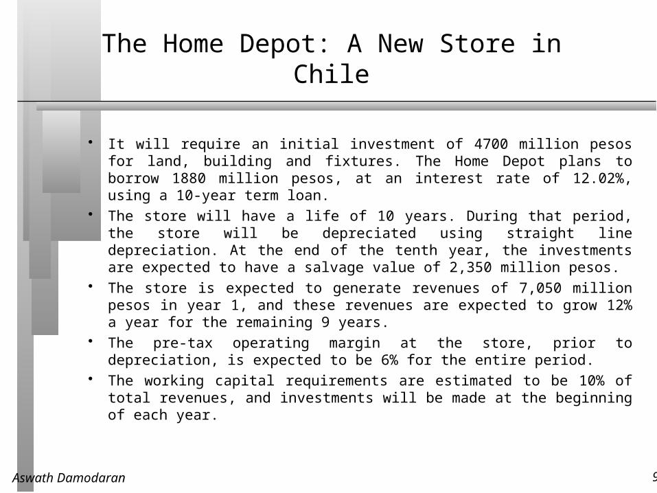
It will require an initial investment of 4700 million pesos for land, building and fixtures. The Home Depot plans to borrow 1880 million pesos, at an interest rate of 12.02%, using a 10-year term loan.

The store will have a life of 10 years. During that period, the store will be depreciated using straight line depreciation. At the end of the tenth year, the investments are expected to have a salvage value of 2,350 million pesos.

The store is expected to generate revenues of 7,050 million pesos in year 1, and these revenues are expected to grow 12% a year for the remaining 9 years.

The pre-tax operating margin at the store, prior to depreciation, is expected to be 6% for the entire period.

The working capital requirements are estimated to be 10% of total revenues, and investments will be made at the beginning of each year.

Aswath Damodaran 94

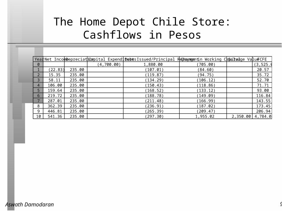
The Home Depot Chile Store: Cashflows in Pesos

Year Net Income Depreciation Capital Expenditures Debt Issued/Principal Repayment Change in Working Capital Salvage Value FCFE0 (4,700.00) 1,880.00 (705.00) (3,525.00)1 (22.83) 235.00 (107.01) (84.60) 20.572 15.35 235.00 (119.87) (94.75) 35.723 58.11 235.00 (134.29) (106.12) 52.704 106.00 235.00 (150.43) (118.86) 71.715 159.64 235.00 (168.52) (133.12) 93.006 219.72 235.00 (188.78) (149.09) 116.847 287.01 235.00 (211.48) (166.99) 143.558 362.39 235.00 (236.91) (187.02) 173.459 446.81 235.00 (265.39) (209.47) 206.94

10 541.36 235.00 (297.30) 1,955.02 2,350.00 4,784.08

Aswath Damodaran 95

The Home Depot Chile Store: Cost of Equity in Pesos

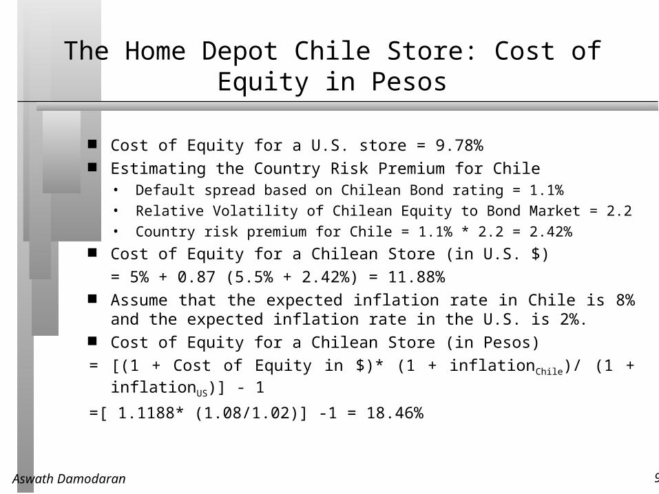
Cost of Equity for a U.S. store = 9.78% Estimating the Country Risk Premium for Chile

• Default spread based on Chilean Bond rating = 1.1%

• Relative Volatility of Chilean Equity to Bond Market = 2.2

• Country risk premium for Chile = 1.1% * 2.2 = 2.42% Cost of Equity for a Chilean Store (in U.S. $)

= 5% + 0.87 (5.5% + 2.42%) = 11.88% Assume that the expected inflation rate in Chile is 8% and the

expected inflation rate in the U.S. is 2%. Cost of Equity for a Chilean Store (in Pesos)

= [(1 + Cost of Equity in $)* (1 + inflationChile)/ (1 + inflationUS)] - 1

=[ 1.1188* (1.08/1.02)] -1 = 18.46%

Aswath Damodaran 96

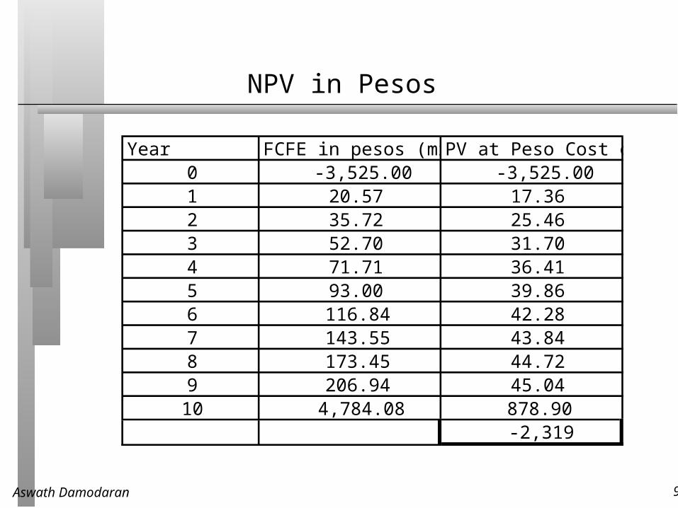
NPV in Pesos

Year FCFE in pesos (millions)PV at Peso Cost of Equity0 -3,525.00 -3,525.001 20.57 17.362 35.72 25.463 52.70 31.704 71.71 36.415 93.00 39.866 116.84 42.287 143.55 43.848 173.45 44.729 206.94 45.04

10 4,784.08 878.90-2,319

Aswath Damodaran 97

Converting Pesos to U.S. dollars

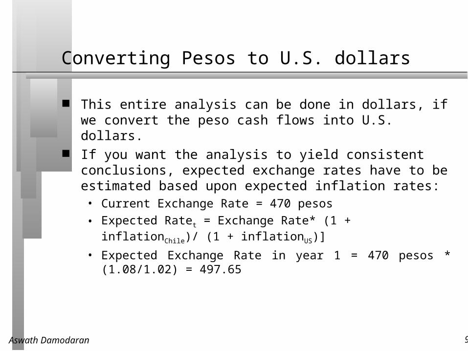
This entire analysis can be done in dollars, if we convert the peso cash flows into U.S. dollars.

If you want the analysis to yield consistent conclusions, expected exchange rates have to be estimated based upon expected inflation rates:• Current Exchange Rate = 470 pesos

• Expected Ratet = Exchange Rate* (1 + inflationChile)/ (1 + inflationUS)]

• Expected Exchange Rate in year 1 = 470 pesos * (1.08/1.02) = 497.65

Aswath Damodaran 98

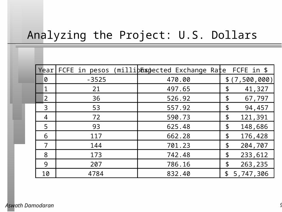
Analyzing the Project: U.S. Dollars

Year FCFE in pesos (millions) Expected Exchange Rate FCFE in $0 -3525 470.00 (7,500,000)$ 1 21 497.65 41,327$ 2 36 526.92 67,797$ 3 53 557.92 94,457$ 4 72 590.73 121,391$ 5 93 625.48 148,686$ 6 117 662.28 176,428$ 7 144 701.23 204,707$ 8 173 742.48 233,612$ 9 207 786.16 263,235$

10 4784 832.40 5,747,306$

Aswath Damodaran 99

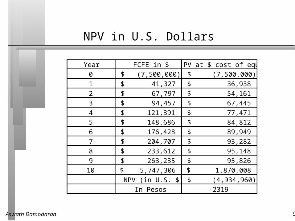
NPV in U.S. Dollars

Year FCFE in $ PV at $ cost of equity0 (7,500,000)$ (7,500,000)$ 1 41,327$ 36,938$ 2 67,797$ 54,161$ 3 94,457$ 67,445$ 4 121,391$ 77,471$ 5 148,686$ 84,812$ 6 176,428$ 89,949$ 7 204,707$ 93,282$ 8 233,612$ 95,148$ 9 263,235$ 95,826$

10 5,747,306$ 1,870,008$ NPV (in U.S. $) (4,934,960)$

In Pesos -2319

Aswath Damodaran 100

The Role of Sensitivity Analysis

Our conclusions on a project are clearly conditioned on a large number of assumptions about revenues, costs and other variables over very long time periods.

To the degree that these assumptions are wrong, our conclusions can also be wrong.

One way to gain confidence in the conclusions is to check to see how sensitive the decision measure (NPV, IRR..) is to changes in key assumptions.


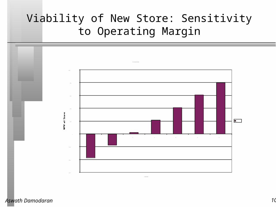
Viability of New Store: Sensitivity to Operating Margin

NPV and Operating Margin

$(6,000)

$(4,000)

$(2,000)

$-

$2,000

$4,000

$6,000

$8,000

$10,000

6% 7% 8% 9% 10% 11% 12%

Operating Margin

NPV


What does sensitivity analysis tell us?

Assume that the manager at The Home Depot who has to decide on whether to take this plant is very conservative. She looks at the sensitivity analysis and decides not to take the project because the NPV would turn negative if the operating margin drops below 8%. Is this the right thing to do?

Yes No

Explain.


Dealing with Inflation

In our analysis, we used nominal dollars and pesos. Would the NPV have been different if we had used real cash flows instead of nominal cash flows?

It would be much lower, since real cash flows are lower than nominal cash flows

It would be much higher It should be unaffected


From Nominal to Real : The Home Depot

To do a real analysis, you need a real cost of equity or capital• Nominal cost of equity for The Home Depot = 9.78%

• Expected Inflation rate = 2%

• Real Cost of Equity = (1.0978/1.02)-1 = 7.59% To estimate cash flows in real terms

• Real Cash flowt = Nominal Cash flowt / (1+ Expected Inflation rate)t


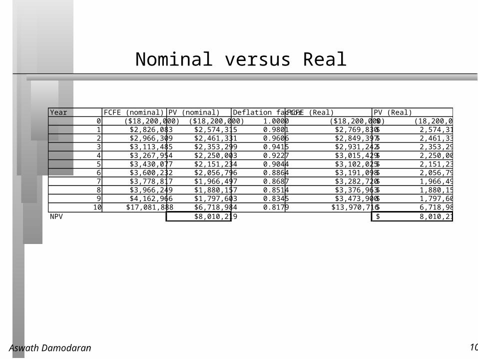
Nominal versus Real

Year FCFE (nominal) PV (nominal) Deflation factor FCFE (Real) PV (Real)0 ($18,200,000) ($18,200,000) 1.0000 ($18,200,000) (18,200,000)$ 1 $2,826,083 $2,574,315 0.9801 $2,769,830 2,574,315$ 2 $2,966,309 $2,461,331 0.9606 $2,849,397 2,461,331$ 3 $3,113,485 $2,353,299 0.9415 $2,931,242 2,353,299$ 4 $3,267,954 $2,250,003 0.9227 $3,015,429 2,250,003$ 5 $3,430,077 $2,151,234 0.9044 $3,102,025 2,151,234$ 6 $3,600,232 $2,056,796 0.8864 $3,191,098 2,056,796$ 7 $3,778,817 $1,966,497 0.8687 $3,282,720 1,966,497$ 8 $3,966,249 $1,880,157 0.8514 $3,376,963 1,880,157$ 9 $4,162,966 $1,797,603 0.8345 $3,473,900 1,797,603$

10 $17,081,888 $6,718,984 0.8179 $13,970,716 6,718,984$ NPV $8,010,219 8,010,219$


Side Costs and Benefits

Most projects considered by any business create side costs and benefits for that business.

The side costs include the costs created by the use of resources that the business already owns (opportunity costs) and lost revenues for other projects that the firm may have.

The benefits that may not be captured in the traditional capital budgeting analysis include project synergies (where cash flow benefits may accrue to other projects) and options embedded in projects (including the options to delay, expand or abandon a project).

The returns on a project should incorporate these costs and benefits.


Opportunity Cost

An opportunity cost arises when a project uses a resource that may already have been paid for by the firm.

When a resource that is already owned by a firm is being considered for use in a project, this resource has to be priced on its next best alternative use, which may be• a sale of the asset, in which case the opportunity cost is the expected

proceeds from the sale, net of any capital gains taxes

• renting or leasing the asset out, in which case the opportunity cost is the expected present value of the after-tax rental or lease revenues.

• use elsewhere in the business, in which case the opportunity cost is the cost of replacing it.


Project Synergies

A project may provide benefits for other projects within the firm. If this is the case, these benefits have to be valued and shown in the initial project analysis.

For instance, the Home Depot, when it considers opening a new restaurant at one of its stores, will have to examine the additional revenues that may accrue to this store from people who come to the restaurant.


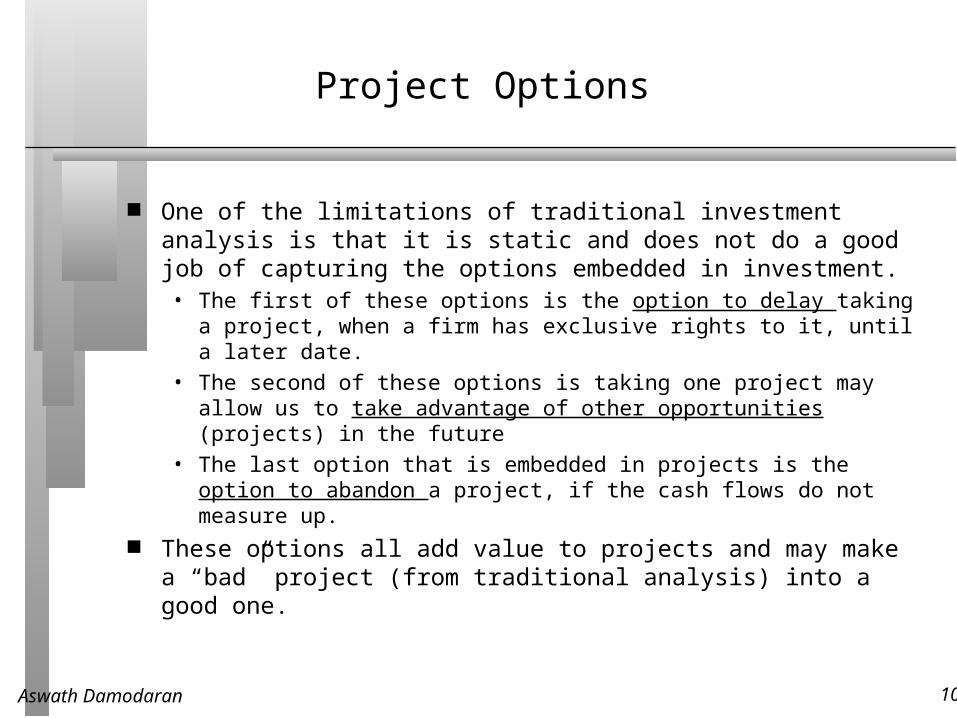
Project Options

One of the limitations of traditional investment analysis is that it is static and does not do a good job of capturing the options embedded in investment.• The first of these options is the option to delay taking a project, when a

firm has exclusive rights to it, until a later date.

• The second of these options is taking one project may allow us to take advantage of other opportunities (projects) in the future

• The last option that is embedded in projects is the option to abandon a project, if the cash flows do not measure up.

These options all add value to projects and may make a “bad” project (from traditional analysis) into a good one.


The Option to Delay

When a firm has exclusive rights to a project or product for a specific period, it can delay taking this project or product until a later date.

A traditional investment analysis just answers the question of whether the project is a “good” one if taken today.

Thus, the fact that a project does not pass muster today (because its NPV is negative, or its IRR is less than its hurdle rate) does not mean that the rights to this project are not valuable.


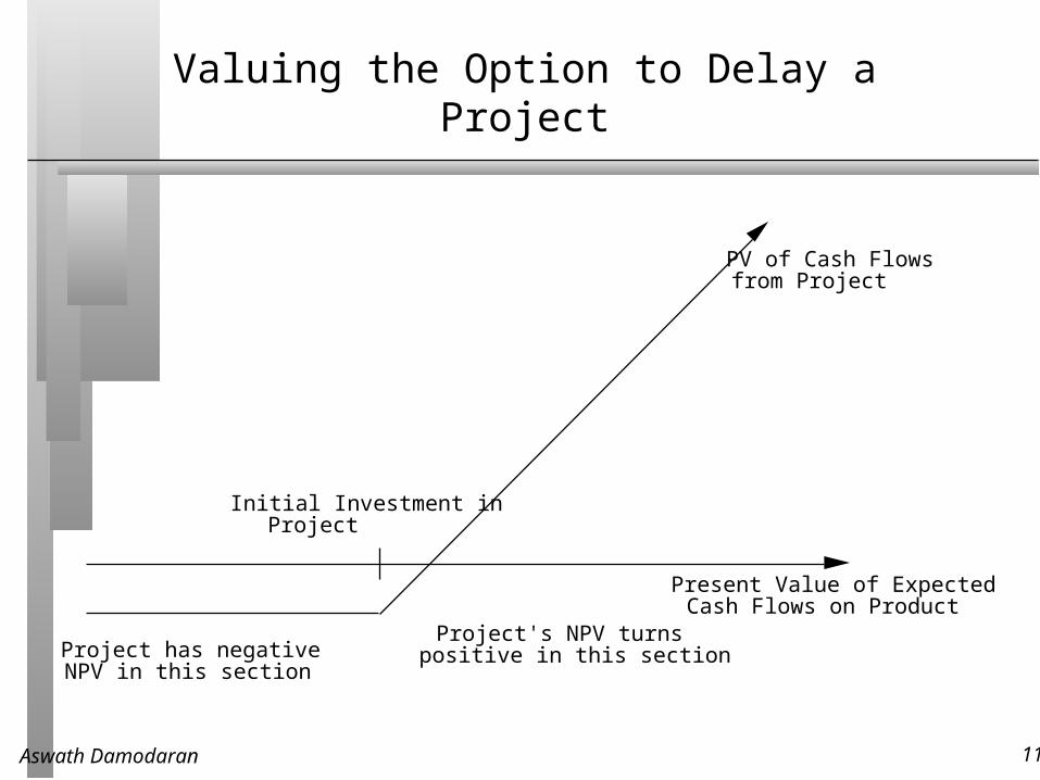
Valuing the Option to Delay a Project

Present Value of Expected Cash Flows on Product

PV of Cash Flows from Project

Initial Investment in Project

Project has negativeNPV in this section

Project's NPV turns positive in this section


Insights for Investment Analyses

Having the exclusive rights to a product or project is valuable, even if the product or project is not viable today.

The value of these rights increases with the volatility of the underlying business.

The cost of acquiring these rights (by buying them or spending money on development - R&D, for instance) has to be weighed off against these benefits.


The Option to Expand/Take Other Projects

Taking a project today may allow a firm to consider and take other valuable projects in the future.

Thus, even though a project may have a negative NPV, it may be a project worth taking if the option it provides the firm (to take other projects in the future) provides a more-than-compensating value.

These are the options that firms often call “strategic options” and use as a rationale for taking on “negative NPV” or even “negative return” projects.


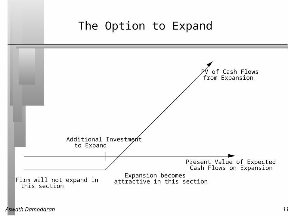
The Option to Expand

Present Value of Expected Cash Flows on Expansion

PV of Cash Flows from Expansion

Additional Investment to Expand

Firm will not expand inthis section

Expansion becomes attractive in this section


An Example of an Expansion Option

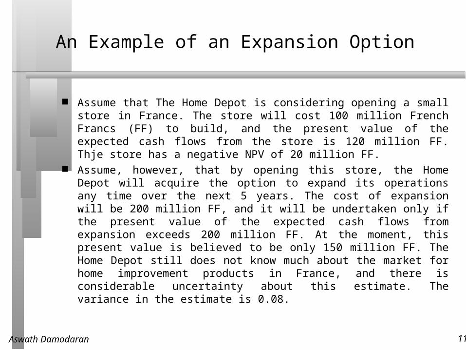
Assume that The Home Depot is considering opening a small store in France. The store will cost 100 million French Francs (FF) to build, and the present value of the expected cash flows from the store is 120 million FF. Thje store has a negative NPV of 20 million FF.

Assume, however, that by opening this store, the Home Depot will acquire the option to expand its operations any time over the next 5 years. The cost of expansion will be 200 million FF, and it will be undertaken only if the present value of the expected cash flows from expansion exceeds 200 million FF. At the moment, this present value is believed to be only 150 million FF. The Home Depot still does not know much about the market for home improvement products in France, and there is considerable uncertainty about this estimate. The variance in the estimate is 0.08.


Valuing the Expansion Option

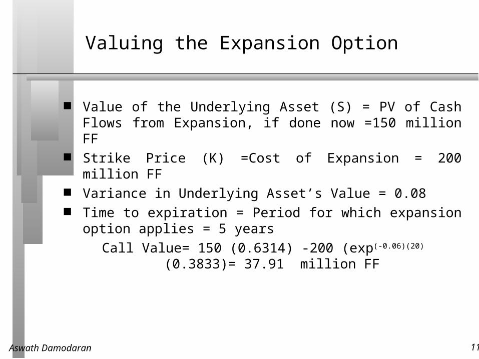
Value of the Underlying Asset (S) = PV of Cash Flows from Expansion, if done now =150 million FF

Strike Price (K) =Cost of Expansion = 200 million FF Variance in Underlying Asset’s Value = 0.08 Time to expiration = Period for which expansion option applies = 5

years

Call Value= 150 (0.6314) -200 (exp(-0.06)(20) (0.3833)= 37.91 million FF


Considering the Project with Expansion Option

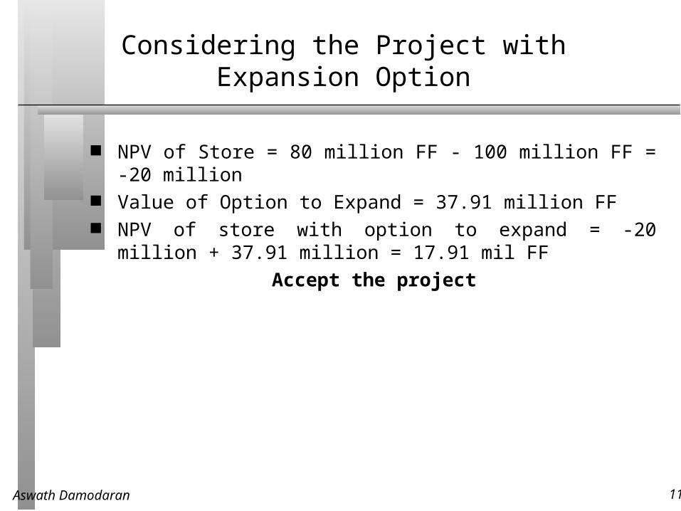
NPV of Store = 80 million FF - 100 million FF = -20 million Value of Option to Expand = 37.91 million FF NPV of store with option to expand = -20 million + 37.91 million =

17.91 mil FF

Accept the project


The Option to Abandon

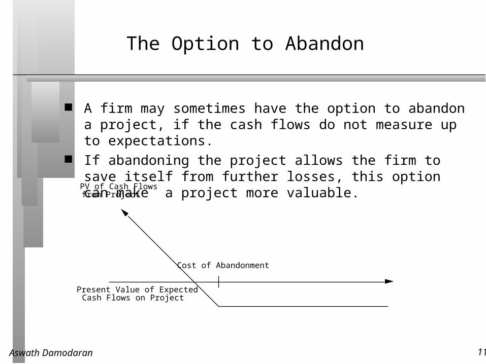
A firm may sometimes have the option to abandon a project, if the cash flows do not measure up to expectations.

If abandoning the project allows the firm to save itself from further losses, this option can make a project more valuable.

Present Value of Expected Cash Flows on Project

PV of Cash Flows from Project

Cost of Abandonment


Valuing the Option to Abandon

Assume that the Home Depot is considering a new store that requires a net initial investment of $ 9.5 million and generates cash flows with a present value of $8.563 million. The net present value of -$937,287 would lead us to reject this project.

To illustrate the effect of the option to abandon, assume that the Home Depot has the option to close the store any time over the next 10 years and sell the land back to the original owner for $ 5 million. In addition, assume that the standard deviation in the present value of the cash flows is 22%.


Project with Option to Abandon

Value of the Underlying Asset (S) = PV of Cash Flows from Project= $ 8,562,713

Strike Price (K) = Salvage Value from Abandonment = $ 5 million Variance in Underlying Asset’s Value = 0.222 = 0.0484 Time to expiration = Life of the Project = 10 years Dividend Yield = 1/Life of the Project = 1/10 = 0.10 (We are

assuming that the project’s present value will drop by roughly 1/n each year into the project)

The riskless rate is 5%.


Should The Home Depot take this project?

Value of Put = 5,000,000 exp(-0.05)(10) (1-0.4977) - -8,562,713 exp(0.10)(10) (1-0.7548) = $ 474,831

The value of this abandonment option has to be added to the net present value of the project of -$ 937,287, yielding a total net present value that remains negative.

NPV without abandonment option = -$937,287

Value of abandonment option = +$474,831

NPV with abandonment option = -$462,456

Notwithstanding the abandonment option, this store should not be opened.


First Principles

Invest in projects that yield a return greater than the minimum acceptable hurdle rate.• The hurdle rate should be higher for riskier projects and reflect the

financing mix used - owners’ funds (equity) or borrowed money (debt)

• Returns on projects should be measured based on cash flows generated and the timing of these cash flows; they should also consider both positive and negative side effects of these projects.

Choose a financing mix that minimizes the hurdle rate and matches the assets being financed.

If there are not enough investments that earn the hurdle rate, return the cash to stockholders.• The form of returns - dividends and stock buybacks - will depend upon

the stockholders’ characteristics.

Documents

Aswath Damodaran1 The Investment Principle Aswath Damodaran Stern School of Business