Asymmetric Effects of Economic Uncertainty on Money Demand

S. M. Woahid Murad International Journal of Business and Economics 20 (2021) 187-199

187

Asymmetric Effects of Economic Uncertainty on Money

Demand Function in Bangladesh: A Nonlinear ARDL

and Cumulative Fourier Causality Approach

S. M. Woahid Murad*

Department of Economics, Noakhali Science and Technology University, Noakhali, Bangladesh

Abstract

This study revisits the demand for money in Bangladesh considering economic

uncertainty and covering 1999:M1 to 2018:M6. We employed a nonlinear ARDL model and

cumulative Fourier causality tests. In contrast to the previous studies, we obtain higher

exchange rate elasticity and lower income elasticity of money demand function. It is found

that people hold less money in the short run when uncertainty increases, albeit it does not

sustain in the long run. On the contrary, demand for money rises in the short run and declines

in the long run when uncertainty decreases. We also find a unidirectional causality from

income and economic uncertainty to money after considering the Fourier causality test.

Therefore, a fiscal policy should be considered along with a monetary policy to tune

Bangladesh’s economy.

Keywords: Money Demand, Output Uncertainty, Nonlinear ARDL, Fourier Causality,

Bangladesh

JEL Classification: C22, E41

* Correspondence to: Department of Economics, Noakhali Science and Technology University,

Noakhali-3814, Bangladesh. Email: [email protected]. The author is grateful to two anonymous

reviewers of this journal for their valuable comments on an earlier draft of this paper. However, the

usual disclaimer would be applied.

mailto:[email protected]


188

1. Introduction

The monetary policy of Bangladesh attempts to stabilize the price level and accelerate

economic growth with job-supportive and eco-friendly strategies. However, stability of the

money demand function is essential for the effectiveness of monetary policy (for instance,

Friedman, 1956).

At the end of the 1970s, the US economy failed to attain the inflation target for three

consecutive years. The quantity theory of money was highly criticized. Therefore, Friedman

(1984) encompassed the volatility of money in his money demand function and explored the

dominant role of monetary uncertainty in determining the demand for money. Later,

Bruggemann and Nautz (1997) reinvestigated Friedman (1984) model in the context of

Germany and found an inverse relationship between monetary uncertainty and demand for

money. On the contrary, Choi and Oh (2003) developed a theoretical framework considering

output uncertainty and monetary uncertainty together in the traditional money demand function.

Using the U.S. data, they reported a negative effect of output uncertainty and a positive effect

of monetary uncertainty on demand for money. It may happen since output uncertainty

generates uncertain job prospects, and, therefore, people allocate their money in less volatile

assets.

Moreover, several studies empirically examined the impact of output volatility on demand

for money, for instance, Hall and Noble (1987), Bahmani-Oskooee and Xi (2011), Bahmani-

Oskooee, Xi, and Wang (2012), Ö zdemir and Saygili (2013), Bahmani-Oskooee,

Satawatananon, and Xi (2015), Bahmani-Oskooee and Arize (2020). However, the effect of

macroeconomic volatility on demand for holding money varies substantially across countries.

Therefore, a country-specific estimation of the money demand function is required to develop

an effective monetary policy of that country.

An extensive number of studies estimated the money demand function for Bangladesh.

For instance, Ahmed (1977), and Murti and Murti (1978) estimated the money demand function

for Bangladesh considering real income and nominal interest rate, while Taslim (1984) chose

expected inflation instead of interest rate, and they obtained a stable money demand function

for Bangladesh. Besides, Ahmed (1999), Siddiki (2000), Hossain (2010) estimated

Bangladesh’s money demand function within an open economy framework. Ahmed (1999)

considered the real exchange rate, while Siddiki (2000), Hossain (2010) regarded it as nominal

exchange rate and nominal effective exchange rate, respectively. All of them found a significant

effect of the exchange rate on demand for money. However, none of the prior empirical studies

considered volatility or uncertainty in estimating the money demand function of Bangladesh.

Consequently, this current study attempts to address the literature gap and examine the

asymmetric effect of economic volatility on the money demand function of Bangladesh.

Moreover, this study also explored the causal relationship among money, income, interest rate,

exchange rate, and economic volatility using cumulative Fourier-frequency.

The rest of the paper’s outline is as follows: Section 2 covers the model’s specification,

data sources, and methodology. Section 3 reports and discusses empirical findings, and finally,

Section 4 provides concluding remarks of this study.

2. Model Specification, Data Sources, and Estimation Methods

As postulated in Keynes (1936), a traditional money demand function expresses demand

for money as a function of income and interest rate. Afterward, Mundell (1963) and Choi and

Oh (2003) augmented the money demand function by adding foreign exchange rate, output


189

uncertainty, respectively. After considering all these improvements together and adding an

error term, the following log-linear empirical model can be specified:

𝑚𝑡 = 𝛽0 + 𝛽1𝑦𝑡 + 𝛽2𝑖𝑡 + 𝛽3𝑠𝑡 + 𝛽4𝑣𝑜𝑙𝑡 + 𝑢𝑡, (1)

where, 𝛽0 = intercept, 𝑚 = real money supply obtained from nominal 𝑀2 deflated by the CPI,

𝑦 = industrial production index (IPI) as a proxy of income, 𝑖 = nominal interest rate obtained

from the money market rate, 𝑠 = real exchange rate of Bangladeshi taka against the US dollar,

𝑣𝑜𝑙 = economic volatility generated from the GARCH effect of the IPI, 𝑡 = time, 𝑢 is an error

term and 𝑢 ≈ 𝑁(0, 𝜎). This study covers monthly data from 1999:M1 to 2018:M6. The starting

and ending period is chosen based on the availability of data of the selected variables. Data is

compiled from the Monthly Economic Trends published by the Bangladesh Bank and the

International Financial Statistics published by the IMF. All of the variables are in the natural

log.

According to the Keynesian and monetarists’ hypotheses, 𝛽1 is expected to be positive,

implying that demand for money increases with income at the cost of foregone interest earnings.

In contrast, the expected sign of 𝛽2 is negative since the interest rate is considered as an

opportunity of holding money. However, the signs of 𝛽3 and 𝛽4 are ambiguous. The coefficient

of the real exchange rate depends on the relative strength of the wealth effect and substitution

effect. During a depreciation of Bangladeshi taka, people are supposed to hold more cash if the

wealth effect outweighs the substitution effect. Finally, the sign of 𝛽4 depends on how people

allocate their money during the uncertain prospect. However, recent empirical studies, for

instance, Bahmani-Oskooee, Halicioglu and Bahmani (2017), Bahmani-Oskooee and Maki-

Nayeri (2019), and Murad, Salim and Kibria (2021), found asymmetric effects of uncertainty

on demand for holding money. For considering asymmetric effects of output uncertainty in

Equation (1), we decompose the uncertainty in cumulative partial sum of positive and negative

values of 𝑣𝑜𝑙 in the following way:

𝑣𝑜𝑙𝑡+ = ∑ ∆𝑣𝑜𝑙𝑖

+ = ∑ 𝑚𝑎𝑥(∆𝑣𝑜𝑙𝑖, 0)𝑡𝑖=1

𝑡𝑖=1 ,

(2) 𝑣𝑜𝑙𝑡− = ∑ ∆𝑣𝑜𝑙𝑖

− = ∑ 𝑚𝑖𝑛(∆𝑣𝑜𝑙, 0)𝑡𝑖=1

𝑡𝑖=1 ,

𝑣𝑜𝑙𝑡 is replaced in Equation (1) by its cumulative partial sums as defined in Equation (2) to examine the asymmetric effect of volatility. To estimate the nonlinear ARDL model, Equation (1) can be restated in the following way:

∆𝑚𝑡 = 𝛼 + ∑ 𝛾𝑖∆𝑚𝑡−𝑖𝑎𝑖=1 + ∑ 𝜂𝑖∆𝑦𝑡−𝑖

𝑏𝑖=1 + ∑ 𝜆𝑖

𝑐𝑖=1 Δ𝑖𝑡−𝑖 + ∑ 𝜑𝑖

𝑑𝑖=1 Δ𝑠𝑡−𝑖 +

∑ 𝜔𝑖+𝑒

𝑖=1 Δ𝑣𝑜𝑙𝑡−𝑖+ + ∑ 𝜔𝑖

−𝑓𝑖=1 Δ𝑣𝑜𝑙𝑡−𝑖

− + 𝜌0𝑚𝑡−1 + 𝜌1𝑦𝑡−1 + 𝜌2𝑖𝑡−1 + 𝜌3𝑠𝑡−1 +𝜌4𝑣𝑜𝑙𝑡−1

+ + 𝜌5𝑣𝑜𝑙𝑡−1− + 휀𝑡,

(3)

where Δ is the first difference operator; 𝛼 is the drift term; 𝑎 to 𝑓 are the optimum lag

lengths selected by the Akaike information criterion (AIC). 𝛾, 𝜂, 𝜆, 𝜑, 𝜔+ and 𝜔− are the

short-run parameters while the estimates of 𝜌1 to 𝜌5 present the long-run effects. The long-run

estimates are normalized on 𝜌0. Finally, 휀𝑡 is the white noise error term.

Before proceeding to estimate the short-run and long-run parameters, one should confirm

that the variables are cointegrated. Pesaran, Shin, and Smith (2001) propose the bounds testing

procedure to identify a cointegrating relationship among the variables. If the calculated 𝐹-

statistic exceeds the critical values of the upper and lower bounds, one can conclude that the

considered variables are cointegrated. Subsequently, Kripfganz and Schneider (2020) develop

critical values for the bounds testing approach through response surface models. Therefore, we


190

have considered both Pesaran, Shin, and Smith (2001) and Kripfganz and Schneider (2020)

critical values to establish a cointegrating relationship among the variables.

A battery of diagnostic tests has been occupied to identify specification bias of the models.

We employ the Breusch-Godfrey LM test, White homoscedasticity test, and Ramsey RESET

test to check the presence of serial correlation, heteroscedasticity, and omitted variable bias

problems, respectively. The skewness and kurtosis tests show the normality of the model.

Finally, the Wald test statistics ensure the short-run and long-run asymmetry.

Furthermore, we incorporate the recently developed Fourier Toda-Yamamoto causality

test with a cumulative frequency of Gormus, Nazlioglu, and Soytas (2019) (hereafter, GNS)

along with Toda and Yamamoto (1995) causality test. These tests help to identify causal

relationships among money, income, interest rate, real exchange rate, and volatility. These

causality tests were incorporated to provide an insight into the Keynesian and monetarists’

debate. More specifically, it will help in concluding the direction of causality between money

and income.

Toda and Yamamoto (1995) postulated Granger causality test is based on the 𝑉𝐴𝑅(𝑝 +𝑑) model, which can be specified as follows

𝑥𝑡 = 𝜃 + ∑ 𝛿𝑖𝑥𝑡−𝑖𝑝+𝑑𝑖=1 + 𝜈𝑡, (4)

where 𝜃 is an intercept vector, 𝑥 is a vector of 𝑘 endogenous variables, 𝛿 is a coefficient

vector, 𝑝 is the lag length and 𝑑 is the maximum order of integration, 𝑡 denotes time, and

finally, 𝜈 is a vector of white noise residuals. Here the null hypothesis is based on zero

restriction on 𝑝 of the 𝑘 th 𝑦 , i.e., 𝐻0: 𝛿1 = ⋯ = 𝛿𝑝 = 0 . The Wald test statistic for this

hypothesis test follows an asymptotic 𝜒2 distribution with 𝑝 degrees of freedom.

To accommodate unknown smooth structural breaks, GNS (2019) utilizes a Fourier series

approximation. Therefore, using Fourier functional form, Equation (4) can be expressed as

𝑥𝑡 = 𝜃0 + 𝜙1sin (2𝜋𝑘𝑡

𝑇) + 𝜙2 cos (

2𝜋𝑘𝑡

𝑇) + ∑ 𝛿𝑖𝑥𝑡−𝑖

𝑝+𝑑𝑖=1 + 𝜈𝑡, (5)

where 𝑘 stands for the approximation frequency, 𝑇 presents the number of observations, 𝜙1

and 𝜙2 measure the amplitude and displacement of the frequency, respectively.

Equation (5) illustrates a Fourier Toda-Yamamoto causality test. However, according to

GNS (2019), the Toda and Yamamoto causality test is suitable for a small sample size (for

example, 𝑇 ≅ 25 ), while a single frequency Fourier Toda-Yamamoto causality test is

appropriate for the sample size between 50 to 100. On the contrary, a cumulative frequency of

the Fourier Toda-Yamamoto causality test yields precise estimations if the number of

observations is around 250. Therefore, we have considered a cumulative frequency of the

Fourier Toda-Yamamoto causality test in our study with the traditional Toda-Yamamoto

causality test.

3. Empirical Findings

Like Pesaran, Shin, and Smith (2001) ARDL bounds testing approach, the nonlinear

ARDL model required all the variables either 𝐼(0) and/or 𝐼(1). Table 1 reports the results of

several unit root tests. Phillips and Perron (1988) test applied the Newey and West estimators

to correct the potential serial correlation problem, while Rodrigues and Taylor (2012) Fourier

GLS test considered nonlinearities and smooth structural breaks in a series. However, both unit


191

root tests ensure that all variables are stationary after taking their first difference. Therefore, it

provides a basis for the nonlinear ARDL test.

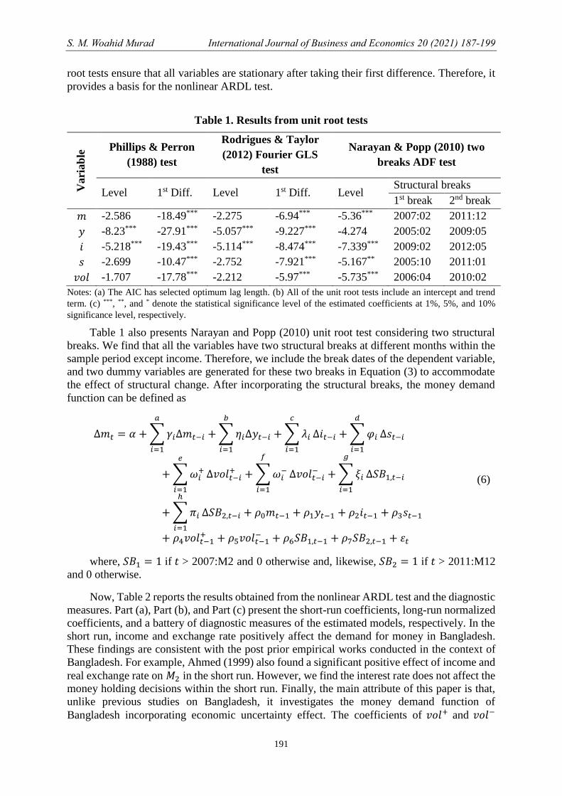
Table 1. Results from unit root tests

Vari

ab

le Phillips & Perron

(1988) test

Rodrigues & Taylor

(2012) Fourier GLS

test

Narayan & Popp (2010) two

breaks ADF test

Level 1st Diff. Level 1st Diff. Level Structural breaks

1st break 2nd break

𝑚 -2.586 -18.49*** -2.275 -6.94*** -5.36*** 2007:02 2011:12

𝑦 -8.23*** -27.91*** -5.057*** -9.227*** -4.274 2005:02 2009:05

𝑖 -5.218*** -19.43*** -5.114*** -8.474*** -7.339*** 2009:02 2012:05

𝑠 -2.699 -10.47*** -2.752 -7.921*** -5.167** 2005:10 2011:01

𝑣𝑜𝑙 -1.707 -17.78*** -2.212 -5.97*** -5.735*** 2006:04 2010:02

Notes: (a) The AIC has selected optimum lag length. (b) All of the unit root tests include an intercept and trend

term. (c) ***, **, and * denote the statistical significance level of the estimated coefficients at 1%, 5%, and 10%

significance level, respectively.

Table 1 also presents Narayan and Popp (2010) unit root test considering two structural

breaks. We find that all the variables have two structural breaks at different months within the

sample period except income. Therefore, we include the break dates of the dependent variable,

and two dummy variables are generated for these two breaks in Equation (3) to accommodate

the effect of structural change. After incorporating the structural breaks, the money demand

function can be defined as

∆𝑚𝑡 = 𝛼 + ∑ 𝛾𝑖∆𝑚𝑡−𝑖

𝑎

𝑖=1

+ ∑ 𝜂𝑖∆𝑦𝑡−𝑖

𝑏

𝑖=1

+ ∑ 𝜆𝑖

𝑐

𝑖=1

Δ𝑖𝑡−𝑖 + ∑ 𝜑𝑖

𝑑

𝑖=1

Δ𝑠𝑡−𝑖

+ ∑ 𝜔𝑖+

𝑒

𝑖=1

Δ𝑣𝑜𝑙𝑡−𝑖+ + ∑ 𝜔𝑖

−

𝑓

𝑖=1

Δ𝑣𝑜𝑙𝑡−𝑖− + ∑ 𝜉𝑖

𝑔

𝑖=1

Δ𝑆𝐵1,𝑡−𝑖

+ ∑ 𝜋𝑖

ℎ

𝑖=1

Δ𝑆𝐵2,𝑡−𝑖 + 𝜌0𝑚𝑡−1 + 𝜌1𝑦𝑡−1 + 𝜌2𝑖𝑡−1 + 𝜌3𝑠𝑡−1

+ 𝜌4𝑣𝑜𝑙𝑡−1+ + 𝜌5𝑣𝑜𝑙𝑡−1

− + 𝜌6𝑆𝐵1,𝑡−1 + 𝜌7𝑆𝐵2,𝑡−1 + 휀𝑡

(6)

where, 𝑆𝐵1 = 1 if 𝑡 > 2007:M2 and 0 otherwise and, likewise, 𝑆𝐵2 = 1 if 𝑡 > 2011:M12

and 0 otherwise.

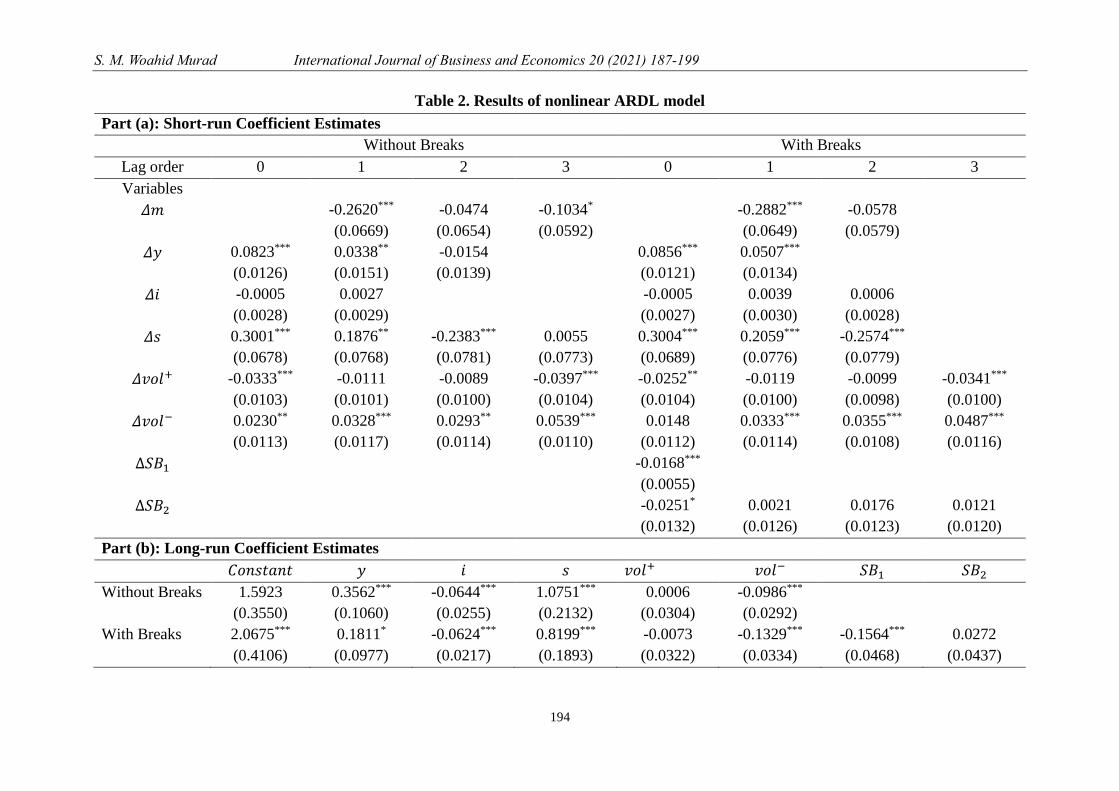
Now, Table 2 reports the results obtained from the nonlinear ARDL test and the diagnostic

measures. Part (a), Part (b), and Part (c) present the short-run coefficients, long-run normalized

coefficients, and a battery of diagnostic measures of the estimated models, respectively. In the

short run, income and exchange rate positively affect the demand for money in Bangladesh.

These findings are consistent with the post prior empirical works conducted in the context of

Bangladesh. For example, Ahmed (1999) also found a significant positive effect of income and

real exchange rate on 𝑀2 in the short run. However, we find the interest rate does not affect the

money holding decisions within the short run. Finally, the main attribute of this paper is that,

unlike previous studies on Bangladesh, it investigates the money demand function of

Bangladesh incorporating economic uncertainty effect. The coefficients of 𝑣𝑜𝑙+ and 𝑣𝑜𝑙−


192

show that people hold less money and probably allocate their money in less risky assets when

volatility increases and, on the contrary, people hold more money when volatility decreases.

Such relation is comparable to Bahmani-Oskooee and Maki-Nayeri (2019). The findings imply

that people’s response to economic uncertainty is counterintuitive to the precautionary effect.

All these findings remain consistent after considering structural breaks. Moreover, structural

changes adversely affect the demand for money.

Part (b) All the long-run estimates are consistent with the theory and empirical studies,

implying a stable money demand function of Bangladesh. Like short-run estimates, the positive

effects of income and exchange rate remain unaltered in the long run. The income elasticity is

less than one, while the exchange rate elasticity is around one. The interest rate effect becomes

significant in the long run, and it has an unfavorable impact on the demand for money.

Specifically, keeping other things equal, people hold about 6% less money if the interest rate

increases by 1%. The long-run coefficients’ signs are consistent with the prior studies, although

their magnitudes differ to some extent. For instance, the long-run income elasticities of broad

money in Islam (2000), and Ahmed and Islam (2005) are 1.60 and 1.89, respectively. In the

case of the USA, Ball (2001) also found that income elasticity was significantly smaller in the

postwar time (1947-94) than the elasticity in the prewar time (1903-45). Fischer (2007) argued

that the income elasticity falls over time because of widening services of financial institutions

(for instance, availability of automatic teller machine or ATM). In contrast to the income

elasticity, the exchange rate elasticity is larger than the previous studies (see Narayan, Narayan,

and Mishra, 2009; Hossain, 2010). Since trade openness, remittance earnings of Bangladesh

increase, the sensitivity of demand for money to the foreign exchange rate also intensifies over

time.

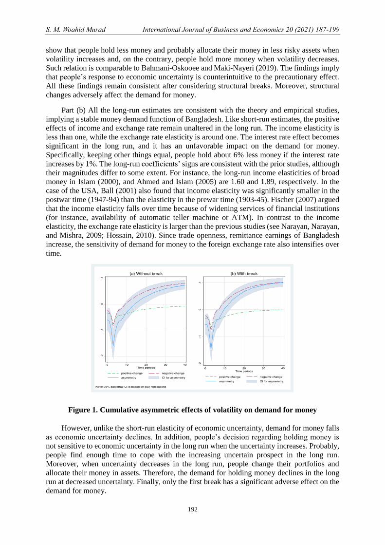
Figure 1. Cumulative asymmetric effects of volatility on demand for money

However, unlike the short-run elasticity of economic uncertainty, demand for money falls

as economic uncertainty declines. In addition, people’s decision regarding holding money is

not sensitive to economic uncertainty in the long run when the uncertainty increases. Probably,

people find enough time to cope with the increasing uncertain prospect in the long run.

Moreover, when uncertainty decreases in the long run, people change their portfolios and

allocate their money in assets. Therefore, the demand for holding money declines in the long

run at decreased uncertainty. Finally, only the first break has a significant adverse effect on the

demand for money.


193

The dynamic asymmetric adjustments of demand for money after positive and negative

shocks of economic uncertainty are also illustrated in Figure 1. According to the dynamic

multiplier, the negative shock has a dominant influence on demand for money.

The calculated 𝐹 and 𝑡 statistics exceed the critical values of Pesaran, Shin, and Smith

(2001) and Kripfganz and Schneider (2020) at 1% and 5% significance levels, respectively.

The ARDL bounds tests confirm that the real cash balance is cointegrated with the considered

variables.


194

Table 2. Results of nonlinear ARDL model

Part (a): Short-run Coefficient Estimates

Without Breaks With Breaks

Lag order 0 1 2 3 0 1 2 3

Variables

𝛥𝑚

-0.2620***

(0.0669)

-0.0474

(0.0654)

-0.1034*

(0.0592)

-0.2882***

(0.0649)

-0.0578

(0.0579)

𝛥𝑦 0.0823***

(0.0126)

0.0338**

(0.0151)

-0.0154

(0.0139)

0.0856***

(0.0121)

0.0507***

(0.0134)

𝛥𝑖 -0.0005

(0.0028)

0.0027

(0.0029)

-0.0005

(0.0027)

0.0039

(0.0030)

0.0006

(0.0028)

𝛥𝑠 0.3001***

(0.0678)

0.1876**

(0.0768)

-0.2383***

(0.0781)

0.0055

(0.0773)

0.3004***

(0.0689)

0.2059***

(0.0776)

-0.2574***

(0.0779)

𝛥𝑣𝑜𝑙+ -0.0333***

(0.0103)

-0.0111

(0.0101)

-0.0089

(0.0100)

-0.0397***

(0.0104)

-0.0252**

(0.0104)

-0.0119

(0.0100)

-0.0099

(0.0098)

-0.0341***

(0.0100)

𝛥𝑣𝑜𝑙− 0.0230**

(0.0113)

0.0328***

(0.0117)

0.0293**

(0.0114)

0.0539***

(0.0110)

0.0148

(0.0112)

0.0333***

(0.0114)

0.0355***

(0.0108)

0.0487***

(0.0116)

∆𝑆𝐵1 -0.0168***

(0.0055)

∆𝑆𝐵2 -0.0251*

(0.0132)

0.0021

(0.0126)

0.0176

(0.0123)

0.0121

(0.0120)

Part (b): Long-run Coefficient Estimates

𝐶𝑜𝑛𝑠𝑡𝑎𝑛𝑡 𝑦 𝑖 𝑠 𝑣𝑜𝑙+ 𝑣𝑜𝑙− 𝑆𝐵1 𝑆𝐵2

Without Breaks 1.5923

(0.3550)

0.3562***

(0.1060)

-0.0644***

(0.0255)

1.0751***

(0.2132)

0.0006

(0.0304)

-0.0986***

(0.0292)

With Breaks 2.0675***

(0.4106)

0.1811*

(0.0977)

-0.0624***

(0.0217)

0.8199***

(0.1893)

-0.0073

(0.0322)

-0.1329***

(0.0334)

-0.1564***

(0.0468)

0.0272

(0.0437)


195

Table 2. Results of nonlinear ARDL model (cont.)

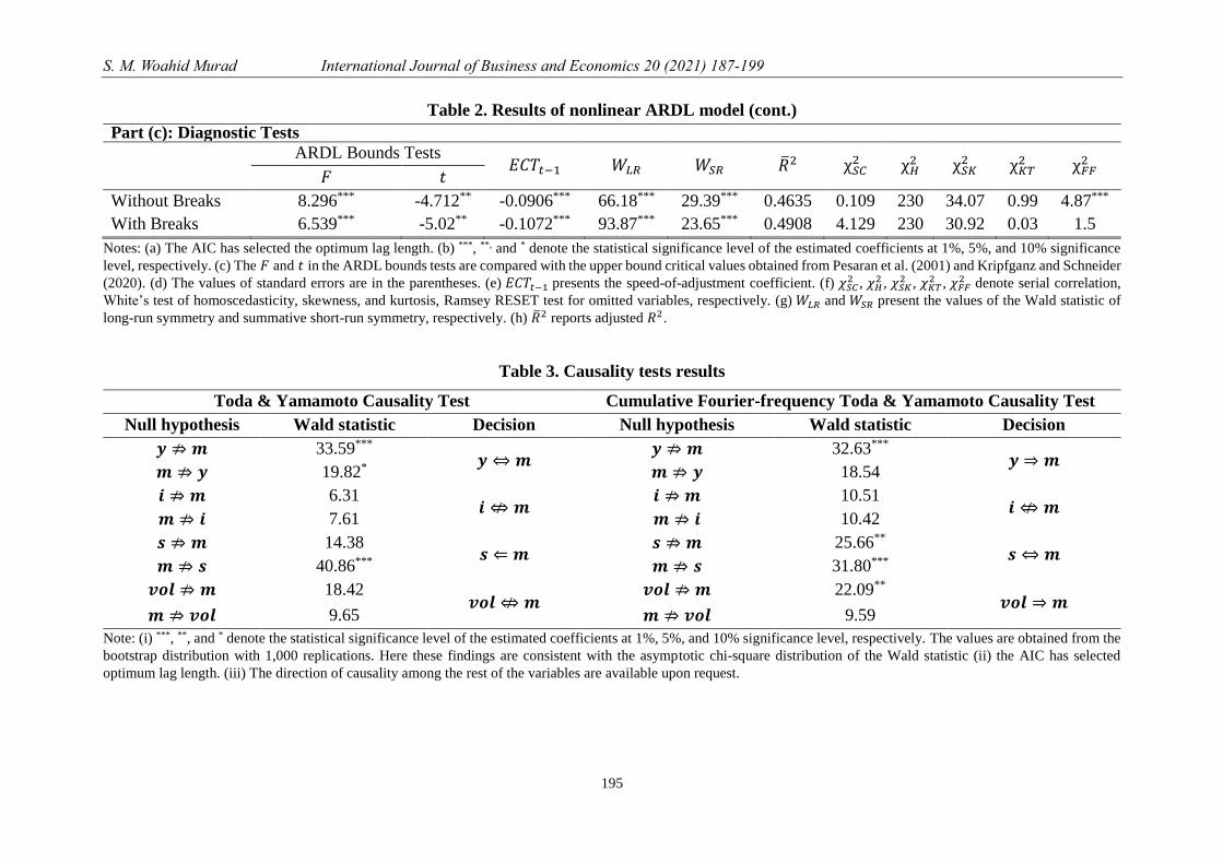
Part (c): Diagnostic Tests

ARDL Bounds Tests

𝐸𝐶𝑇𝑡−1 𝑊𝐿𝑅 𝑊𝑆𝑅 ��2 χ𝑆𝐶2 χ𝐻

2 χ𝑆𝐾2 χ𝐾𝑇

2 χ𝐹𝐹2

𝐹 𝑡

Without Breaks 8.296*** -4.712** -0.0906*** 66.18*** 29.39*** 0.4635 0.109 230 34.07 0.99 4.87***

With Breaks 6.539*** -5.02** -0.1072*** 93.87*** 23.65*** 0.4908 4.129 230 30.92 0.03 1.5

Notes: (a) The AIC has selected the optimum lag length. (b) ***, **, and * denote the statistical significance level of the estimated coefficients at 1%, 5%, and 10% significance

level, respectively. (c) The 𝐹 and 𝑡 in the ARDL bounds tests are compared with the upper bound critical values obtained from Pesaran et al. (2001) and Kripfganz and Schneider

(2020). (d) The values of standard errors are in the parentheses. (e) 𝐸𝐶𝑇𝑡−1 presents the speed-of-adjustment coefficient. (f) 𝜒𝑆𝐶2 , 𝜒𝐻

2 , 𝜒𝑆𝐾2 , 𝜒𝐾𝑇

2 , 𝜒𝐹𝐹2 denote serial correlation,

White’s test of homoscedasticity, skewness, and kurtosis, Ramsey RESET test for omitted variables, respectively. (g) 𝑊𝐿𝑅 and 𝑊𝑆𝑅 present the values of the Wald statistic of

long-run symmetry and summative short-run symmetry, respectively. (h) ��2 reports adjusted 𝑅2.

Table 3. Causality tests results

Toda & Yamamoto Causality Test Cumulative Fourier-frequency Toda & Yamamoto Causality Test

Null hypothesis Wald statistic Decision Null hypothesis Wald statistic Decision

𝒚 ⇏ 𝒎 33.59*** 𝒚 ⇔ 𝒎

𝒚 ⇏ 𝒎 32.63*** 𝒚 ⇒ 𝒎

𝒎 ⇏ 𝒚 19.82* 𝒎 ⇏ 𝒚 18.54

𝒊 ⇏ 𝒎 6.31 𝒊 ⇎ 𝒎

𝒊 ⇏ 𝒎 10.51 𝒊 ⇎ 𝒎

𝒎 ⇏ 𝒊 7.61 𝒎 ⇏ 𝒊 10.42

𝒔 ⇏ 𝒎 14.38 𝒔 ⇐ 𝒎

𝒔 ⇏ 𝒎 25.66** 𝒔 ⇔ 𝒎

𝒎 ⇏ 𝒔 40.86*** 𝒎 ⇏ 𝒔 31.80***

𝒗𝒐𝒍 ⇏ 𝒎 18.42 𝒗𝒐𝒍 ⇎ 𝒎

𝒗𝒐𝒍 ⇏ 𝒎 22.09** 𝒗𝒐𝒍 ⇒ 𝒎

𝒎 ⇏ 𝒗𝒐𝒍 9.65 𝒎 ⇏ 𝒗𝒐𝒍 9.59

Note: (i) ***, **, and * denote the statistical significance level of the estimated coefficients at 1%, 5%, and 10% significance level, respectively. The values are obtained from the

bootstrap distribution with 1,000 replications. Here these findings are consistent with the asymptotic chi-square distribution of the Wald statistic (ii) the AIC has selected

optimum lag length. (iii) The direction of causality among the rest of the variables are available upon request.


196

The error correction terms (𝐸𝐶𝑇𝑡−1) are significant at a 1% significance level and have

expected negative signs. The speed of adjustment is about 10% each month. Consequently, the

adjustment process takes less than one year to restore its long-run equilibrium. The Wald test

statistics support short-run and long-run asymmetric effects of economic uncertainty since their

estimates are significant at a 1% significance level. Except for the Ramsey RESET test, the rest

of the diagnostic measures support that Equation (3) is correctly specified. 𝜒𝐹𝐹2 shows that

either the model commits incorrect functional form or excludes relevant variable(s) from the

model. However, such misspecification disappears as the structural breaks are included in

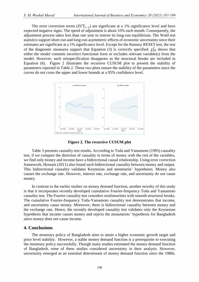
Equation (6). Figure 2 illustrates the recursive CUSUM plot to present the stability of

parameters reported in Table 2. These two plots ensure the stability of the parameters since the

curves do not cross the upper and lower bounds at a 95% confidence level.

Figure 2. The recursive CUSUM plot

Table 3 presents causality test results. According to Toda and Yamamoto (1995) causality

test, if we compare the direction of causality in terms of money with the rest of the variables,

we find only money and income have a bidirectional causal relationship. Using error correction

framework, Hossain (2011) also found such bidirectional causality between money and output.

This bidirectional causality validates Keynesian and monetarist’ hypotheses. Money also

causes the exchange rate. However, interest rate, exchange rate, and uncertainty do not cause

money.

In contrast to the earlier studies on money demand function, another novelty of this study

is that it incorporates recently developed cumulative Fourier-frequency Toda and Yamamoto

causality test. The Fourier causality test considers nonlinearities with smooth structural breaks.

The cumulative Fourier-frequency Toda-Yamamoto causality test demonstrates that income,

and uncertainty cause money. Moreover, there is bidirectional causality between money and

the exchange rate. Hence, the recently developed causality test validates only the Keynesian

hypothesis that income causes money and rejects the monetarists’ hypothesis for Bangladesh

since money does not cause income.

4. Conclusions

The monetary policy of Bangladesh aims to attain a higher economic growth target and

price level stability. However, a stable money demand function is a prerequisite to executing

the monetary policy successfully. Though many studies estimated the money demand function

of Bangladesh, none of these studies considered uncertainty in their analysis. However,

uncertainty emerged as an essential determinant of money demand function since the 1980s.


197

Therefore, we consider output uncertainty in estimating the demand for holding money in this

study, covering monthly data from 1999:M1 to 2018:M6. We employ recently developed time

series econometrics tools.

We find that output and exchange rate have positive and statistically significant effects on

the demand for money in the short and long run. Comparing to the earlier studies, we find that

income elasticity decreases while exchange rate elasticity increases. The favorable exchange

rate effect implies that the wealth effect dominates the substitution effect in liquidity preference.

On the contrary, the demand function is not sensitive to interest rate within the short run.

However, it negatively affects the demand function in the long run. Consequently, the interest

rate is merely a long-run phenomenon in Bangladesh’s money demand function. It implies that

people do not promptly respond to the interest rate.

We find asymmetric effects of income uncertainty on Bangladesh’s money demand

function in the short run and long run. People hold less money and probably invest money in

low volatile assets in the short run when uncertainty increases. However, the significant effect

of increased uncertainty is a short-run phenomenon; it does not sustain in the long run. Unlike

increased uncertainty, liquidity preference induces in the short run and declines in the long run

when uncertainty decreases. The Wald test statistics also support the asymmetric effect, and the

dynamic multiplier illustrates that the negative uncertainty is dominant in determining the

liquidity preference.

Considering the debate between the Keynesian and monetarist schools of thought about

the direction of causality between money and income, we find bidirectional causality when we

disregard nonlinearities and smooth structural breaks. On the contrary, a unidirectional

causality from income to money is found when we allow smooth breaks. Consequently, the

Keynesian hypothesis is robust for Bangladesh.

This study considers only output uncertainty in estimating the money demand function of

Bangladesh. In addition, one can further investigate the money demand function considering

monetary uncertainty (for instance, Friedman, 1984; Hall and Noble, 1987), interest rate

uncertainty (for example, Baba, Hendry and Starr, 1992).

Overall, the demand for broad money in Bangladesh is stable, and uncertainty should be

included in estimating the money demand function since it has both short-run and long-run

impacts. Policymakers can undertake monetary policy to achieve the macroeconomic target.

However, as we find little evidence for monetarist’s hypothesis regarding the direction of

causality from money to income, fiscal policy may be considered along with a monetary policy

to tune the economy.


198

References

Ahmed, N., (1999), “The Demand for Money in Bangladesh During 1975-1997: A

Cointegration Analysis,” Indian Economic Review, 34(2), 171-185.

Ahmed, S., (1977), “Demand for Money in Bangladesh: Some Preliminary Evidences,” The

Bangladesh Development Studies, 5(2), 227-237.

Ahmed, S. and M.E. Islam, (2005), “Demand for Money in Bangladesh: A Cointegration

Analysis,” Bangladesh Development Studies, 31(1-2), 103-120.

Baba, Y., D. F. Hendry, and R. M. Starr, (1992), “The Demand for M1 in the U.S.A., 1960-

1988,” Review of Economic Studies, 59, 25-61.

Bahmani-Oskooee, M. and A.C. Arize, (2020), “On the Asymmetric Effects of Exchange Rate

Volatility on Trade Flows: Evidence from Africa,” Emerging Markets Finance and Trade,

56(4), 913-939.

Bahmani-Oskooee, M., and M. Maki-Nayeri, (2019), “Asymmetric Effects of Policy

Uncertainty on the Demand for Money in the United States,” Journal of Risk and Financial

Management, 12(1).

Bahmani-Oskooee, M., D. Xi and Y. Wang, (2012), “Economic and Monetary Uncertainty and

the Demand for Money in China,” Chinese Economy, 45(6), 26–37.

Bahmani-Oskooee, M., F. Halicioglu and S. Bahmani, (2017), “Do Exchange Rate Changes

Have Symmetric or Asymmetric Effects on the Demand for Money in Turkey?” Applied

Economics, 49(42), 4261-4270.

Bahmani-Oskooee, M., K. Satawatananon and D. Xi, (2015), “Economic Uncertainty,

Monetary Uncertainty, and the Demand for Money in Thailand,” Global Business and

Economics Review, 17(4), 467-476.

Bahmani‐Oskooee, M. and D. Xi, (2011), “Economic Uncertainty, Monetary Uncertainty and

the Demand for Money in Australia,” Australian Economic Papers, 50(4), 115-128.

Ball, L., (2001), “Another Look at Long-run Money Demand,” Journal of Monetary

Economics,” 47, 31–44.

Brüggemann, I., and D. Nautz, (1997), “Money Growth Volatility and the Demand for Money

in Germany: Friedman’s volatility hypothesis revisited,” Review of World Economics,

133(3), 523-537.

Choi, W. G. and S. Oh, (2003), “A Money Demand Function with Output Uncertainty,

Monetary Uncertainty, and Financial Innovations,” Journal of Money, Credit, and Banking,

35(5), 685-709.

Fischer, A. M., (2007), “Measuring Income Elasticity for Swiss Money Demand: What Do the

Cantons Say about Financial Innovation?” European Economic Review, 51(7), 1641-1660.

Friedman, M., (1956), The Quantity Theory of Money - A Restatement. In Studies in the

Quantity Theory of Money, edited by Milton Friedman, 3-21. Chicago: University of

Chicago Press.

Friedman, M., (1984), “Lessons from the 1979-1982 Monetary Policy Experiment,” American

Economic Review, 74(2), 382-387.

Gormus, A., S. Nazlioglu and U. Soytas, (2019), “High-yield Bond and Energy Markets,”

Energy Economics, 69, 101-110.


199

Hall, T. and N. Noble, (1987), “Velocity and the Variability of Money Growth: Evidence from

Granger-Causality Tests: Note,” Journal of Money, Credit and Banking, 19(1), 112-116.

Hossain, A. A., (2010), “Monetary Targeting for Price Stability in Bangladesh: How Stable Is

Its Money Demand Function and the Linkage between Money Supply Growth and

Inflation?” Journal of Asian Economics, 21(6), 564-578

Hossain, M.A., (2011), “Money-Income Causality in Bangladesh: An Error Correction

Approach,” Bangladesh Development Studies, 34(1), 39-58.

Islam, M. A., (2000), “Money demand function for Bangladesh. Bangladesh Development

Studies,” 26(4), 89–111.

Keynes, J. M., (1936), The General Theory of Employment, Interest and Money. London,

Macmillan.

Kripfganz, S. and D. Schneider, (2020), “Response Surface Regressions for Critical Value

Bounds and Approximate p-values in Equilibrium Correction Models,” Oxford Bulletin of

Economics and Statistics, 82(6), 1456-1481.

Mundell, A. R., (1963), “Capital Mobility and Stabilization Policy under Fixed and Flexible

Exchange Rates,” Canadian Journal of Economics and Political Science, 29(4), 475-85.

Murad, S.M.W., R. Salim and M.G. Kibria, (2021), “Asymmetric Effects of Economic Policy

Uncertainty on the Demand for Money in India,” Journal of Quantitative Economics, 19.

Murti, G.V.S.N. and S. Murti, (1978), “The Functional Form of Demand for Money in

Bangladesh,” Bangladesh Development Studies, 6(4), 443-460.

Narayan, P.K. and S. Popp, (2010), “A New Unit Root Test with Two Structural Breaks in

Level and Slope at Unknown Time,” Journal of Applied Statistics, 37(9), 1425-1438.

Narayan, P.K., S. Narayan and V. Mishra, (2009), “Estimating money demand functions for

South Asian countries,” Empirical Economics, 36, 685–696.

Ö zdemir, K. and M. Saygili, (2013), “Economic Uncertainty and Money Demand Stability in

Turkey,” Journal of Economic Studies, 40(3), 314-333.

Pesaran, M. H., Y. Shin and R. J. Smith, (2001), “Bounds Testing Approaches to the Analysis

of Level Relationships,” Journal of Applied Econometrics, 16(3), 289-326.

Phillips, P. C. B., and P. Perron, (1988), “Testing for a Unit Root in Time Series Regression,”

Biometrika, 75, 335–346.

Rodrigues, P. M. and A.M.R. Taylor, (2012), “The Flexible Fourier Form and Local

Generalised Least Squares De‐trended Unit Root Tests,” Oxford Bulletin of Economics and

Statistics, 74(5), 736-759.

Siddiki, J. U, (2000), “Demand for Money in Bangladesh: A Cointegration Analysis,” Applied

Economics, 32(15), 1977-1987.

Taslim, M.A., (1984), “On Rate of Interest and Demand for Money in LDCs: The Case of

Bangladesh,” The Bangladesh Development Studies, 12(3), 19-36.

Toda, H.Y. and T. Yamamoto, (1995), “Statistical Inference in Vector Autoregression with

Possibly Integrated Processes,” Journal of Econometrics, 66(1-2), 225–250.

Documents

Asymmetric Effects of Economic Uncertainty on Money Demand