Asymmetric Information in the Stock Market:Economic News and Co-movement∗

Rui Albuquerque† Clara Vega‡

January 16, 2006

Abstract

We analyze the effect that real-time domestic and foreign news about fundamentalshave on the correlation of stock returns of a small open economy, Portugal, and a largeopen economy, the U.S. We also study the role of public and private information in the priceformation process in the U.S. and Portuguese stock markets. Consistent with our theoreticalmodel, we find that U.S. macroeconomic news and Portuguese earnings news do not affectthe cross-country stock market correlation, whereas Portuguese macroeconomic news lowersthe cross-country stock market correlation. U.S. public information affects Portuguese stockmarket returns, but this effect is diminished when U.S. stock market returns are includedin the regression. This means that part of the co-movement between the U.S. and Portugalis due to the effect that U.S. macroeconomic fundamentals have on the Portuguese stockmarket. Finally, public information news in the U.S. is associated with increased liquidity,while the effect in Portugal depends on the type of news releases.

Keywords: Private information, public news announcements, information spillovers, in-ternational equity returns, contagion.

∗Paper prepared for the conference “Desenvolvimento Económico Português no Espaço Europeu.” We thankAntónio Antunes for providing us with the Portuguese stock market data, Jose Mata for providing us with themacroeconomic news release schedules and the Banco de Portugal for funding this research. The usual disclaimerapplies.

†Boston University School of Management and CEPR. Address at BU: Finance and Economics, 595 Com-monwealth Avenue, Boston, MA 02215. Email: ralbuque@bu.edu. Tel.: 617-353-4614.

‡Board of Governors Federal Reserve System and William E. Simon School of Management. Address: Wash-ington, DC 20551 USA. E-mail: clara.vega@frb.gov. Tel.: 202-452-2379.

1 Introduction

What drives the cross-country correlation of stock returns? This question, central to manytopics in international finance, is deeply associated with another fundamental question: whatis the role of public and private information in the price formation process? Under marketefficiency, information about future stock prices in one market spreads to other markets whereit can also be used to forecast local prices. Cross-country stock return correlations thus arisefrom correlated fundamentals. However, the empirical link between economic fundamentals andcross-country correlations has by and large eluded researchers, leading some to explore contagionas the main driver of stock market correlations. Uncovering the nature of cross-country stockreturn correlations is especially relevant for the development and stability of emerging stockmarkets that are less liquid, more volatile and have a small and fragile investor base: contagionis likely to increase volatility and decrease the investor base, forcing smaller investors out ofthe market.

This paper revisits theoretically and empirically the link between cross-country correlationsand fundamentals and the price discovery process. The standard view in the literature is thatshocks to global factors lead to increases in stock return correlations as they move the valueof firms around the globe in the same direction. Under this view it is then puzzling that thecross-country correlation of returns is the same on U.S. news announcement days and non-announcement days. To the extent that shocks to global factors are shocks to fundamentals, itis also puzzling that U.S. public macroeconomic news affect returns in other countries only ifthe U.S. return is not included in the regression.1

We present a simple model of stock trading, which draws on the work of Kyle (1985) andKing and Wadhwani (1990), that rationalizes the observed, puzzling patterns. In the modelthere is one large, foreign country, and one small, local country. The stock price of the largecountry is driven by a global factor and the stock price of the small country is driven by twofactors, a global factor and a country-specific factor. For simplicity of exposition let the largecountry be the U.S. and the small country be Portugal. Investors in the U.S. are assumednot to respond to news from Portugal,2 but the converse does not apply. Each country isindependently populated with informed investors, noise traders, and a competitive marketmaker. In the model, stock return comovement arises as a result of market efficiency: investorsin Portugal use U.S. returns to infer the private information of U.S. informed investors about theglobal factor. In days with high private information signals about U.S. assets, U.S. net orderflow is positive and so are U.S. returns. Since fundamentals are correlated across countries,this information is good news for the Portuguese stock market and prices rise locally as well.Thus, Portuguese and U.S. stock market returns move together even in the absence of public

1We review the related literature below.2They might recognize its value, but it is assumed that the costs of processing this information (and that

originating from many other small countries) outweight the benefits, and the information is not used in the spiritof Grossman and Stiglitz (1980).

1

announcements.The model predicts that this baseline return comovement should not change in days of U.S.

public news announcements. The effect of Portuguese news on comovement depends on thecontent of the news. If the news are correlated with U.S. valuations (Portuguese macroeconomicnews), then comovement declines on news days, but if the news are country-specific (earningsannouncements) there is no change in this comovement.3 The main assumption for these resultsis the asymmetric response to Portuguese news by investors: U.S. public news releases generateprice discovery in both U.S. and Portuguese markets, whereas Portuguese news releases generateprice discovery in the local market only. Consider first the effects of macroeconomic Portuguesenews announcements. The absence of price discovery in the U.S. market implies that Portugueseinvestors know that trading by U.S. informed investors is not contaminated by the local news.In the context of our model this means that local macroeconomic news can, among otherthings, improve on the information content of U.S. returns leading to a decline in cross-countrycorrelations. Consider now the effect of Portuguese earnings news on comovement. The natureof the news assumes that the mechanism just described is absent and comovement is thereforenot affected. Finally, consider the effects of U.S. news announcements. Price discovery in theU.S. market means that informed U.S. investors ‘subtract’ the public news from their privateinformation and trade only on the remaining portion. Therefore, investors in the Portuguesemarket can no longer use the (same foreign) news to improve on the information content of U.S.returns and cross-country correlations are unchanged. The paper thus provides a theoreticalexplanation for why cross-country correlations of returns do not change after U.S. public newsannouncements and makes additional predictions on how comovement should change based onlocal news.

The model also explains why the U.S. return empirically subsumes the information contentof macroeconomic news releases in the U.S. in driving foreign returns. The reason is that theU.S. return is a sufficient statistic for U.S. public and private information. Finally, the modelpredicts that market liquidity should increase in response to news announcements in the samemarket. The reason is that in a Kyle (1985) model the public news ‘destroys’ some of the valueof the private information. In turn, the market maker is less concerned about adverse selectionand liquidity increases.

We conduct our empirical analysis studying comovement between Portugal and the U.S.We focus on Portuguese stock market data for two main reasons. First, the globalization of theworld economy and in particular the process of European integration means that the Portuguese

3Portuguese firm-specific earnings announcements are not orthogonal to U.S. valuations. However, to em-pirically test our model we need to condition on public announcements that reveal relatively more informationabout country-specific factors than about global factors. The PSI-20 equal weighted and value weighted earningsare not significantly correlated with U.S. GDP growth, while Portuguese GDP growth is significantly correlatedwith U.S. GDP growth. Hence, in our empirical test we interpret Portuguese macroeconomic news as publicannouncements that are correlated with U.S. valuations, while earnings announcements predominantly reveal in-fomation about country-specific factors. In other words, earnings announcements are “nearly” country-specific,in Poterba’s (1990) terminology.

2

stock market is increasingly more vulnerable to external shocks. However, given the relativesizes of the U.S. and Portuguese economies, shocks to the Portuguese economy are not likelyto affect the U.S. This makes it an interesting research laboratory to study how the smallPortuguese stock market responds to economic news at home and abroad (from the U.S.) andallows us to avoid the endogeneity problem associated with the comovement literature. Second,a unique feature of the Portuguese data is that it contains signed trades.4 There is thus no needto rely on artificial algorithms which add measurement error to estimated order flow imbalances.

In testing the hypothesis of our model we use real-time U.S. and Portuguese macroeconomicannouncements and high frequency stock market returns. Such high frequency data allows us toprobe the workings of the marketplace in powerful ways because: (i) we avoid problems relatedto the existence of non-synchronous trading periods between countries (Karolyi and Stulz, 1996);(ii) we measure more accurately the effect that macroeconomic news announcements have onU.S. and Portuguese prices (Andersen et al., 2003) by focusing on episodes where the source ofprice revisions is well identified, thus leading to a high signal-to-noise ratio; (iii) we are ableto test the theoretical assumption that foreign news are first incorporated into foreign stockprices and then they are incorporated into local stock prices; (iv) we measure unanticipatedorder flow which proxies for private information-based trading and are thus able to analyze theeffects of public news conditional on private information.

Consistent with our assertion that the Portuguese stock market is vulnerable to globalshocks, we find that U.S. public macroeconomic news surprises affect the individual componentsof the Portuguese PSI-20 stock market index. As in previous studies, these announcementslose some of their statistical significance when we include the DJ-30 Industrial value weightedindex.5 According to our model, this suggests that part of the comovement between the U.S.and Portugal is due to the effect that U.S. macroeconomic fundamentals have on the Portuguesestock market.

While U.S. macroeconomic news affect Portuguese returns, consistent with previous find-ings, these news do not affect the correlation of stock returns across the two countries. Thesame is true for Portuguese earnings announcements. However, in days of Portuguese macro-economic news there is significantly lower comovement of returns. These last two facts add toour knowledge of comovement of returns as most other studies have focused on news from theU.S. alone. Also, all three facts are consistent with the model developed here.

We also empirically show that U.S. macroeconomic news are first incorporated into U.S.stock market returns and 5 to 15 minutes later they are incorporated into Portuguese stockmarket returns. This empirical evidence supports the assumed timing of the model that Por-tuguese investors incorporate changes in U.S. returns into their trading, and to the best of

4One notable exception is the TORQ database, which contains signed trades for a sample of 144 NYSE stocksfor the three months November, 1990 through January 1991. The advantage of our dataset is that we have nineand a half months of data from January 4, 2002 to October 15, 2002.

5The actual DJ-30 Industrial index is a price weighted measure. In this paper, we construct our own indexusing individual daily stock returns and taking a value weighted average.

3

our knowledge it has not been documented before because previous literature has focused onfrequencies lower than five-minute returns. Interestingly, news on the benchmark interest ratefrom the European Central Bank—the Portuguese Central Bank does not have control over itsown monetary policy—affect U.S. stock market returns and price discovery takes place first inthe U.S. stock market and then in the Portuguese stock market.6 One possible explanationis that price discovery takes place first in the most liquid market, the U.S. stock market (seeHasbrouck (2003)). Another possible explanation is that the opening of the U.S. market coin-cides with the end of the press conference of the ECB and the Reuters release on the ECB’spress conference so the response of the Portuguese stock market is tied to the later fact not theformer.

Finally, public information news in the U.S. increases liquidity in the U.S. market and thesame is true for earnings announcements and liquidity in the Portuguese market. While theseobservations are consistent with our model, we also find that Portuguese macroeconomic newsdecrease liquidity in the Portuguese market. One explanation for this unexpected behavior ofliquidity is that Portuguese macroeconomic news necessitate more analysis to be useful, leadingto the entry into the market of a different class of informed investors (see Kim and Verrecchia(1994)).

We proceed as follows. Next we give a brief literature review. In Section 3, we construct amodel of trading to guide our empirical analysis. In Section 5, we describe the data. In Section6, we present the empirical results and Section 7 concludes. The appendix contains the proofsof the results in the main text.

2 Related Literature

Our paper is most closely related to two areas of research. The first examines internationalasset market linkages and the second highlights the role of order flow in the price formationprocess. In this paper, the two are related because we take the view that both internationalinformation spillovers and order flow are important in the price discovery process. We brieflydiscuss these research areas in turn.

One approach to studying international asset market linkages is to assess the effect of macro-economic news announcements on asset returns around the world. Becker, Finnerty and Fried-man (1995) use high-frequency futures data from 1986 to 1990 and document that U.K. stockmarket returns react to U.S. and U.K. macroeconomic news, while the U.S. stock market onlyreacts to U.S. own news. Wongswan (2005) uses high-frequency data from 1995 to 2000 toshow that there is evidence of transmission of information from the U.S. and Japan to theequity markets in Korea and Thailand. Ehramann and Fratzscher (2003) model the degree ofinterdependence of the U.S. and European interest rate markets by focusing on the reaction of

6Ehramann and Fratzscher (2003) show that ECB monetary policy surprises affect U.S. interest rate markets.Perhaps not surprisingly then we observe that they also affect U.S. stock market returns.

4

these markets to macroeconomic news and monetary policy announcements. They show thatthe connection of the Euro area and the U.S. money markets has steadily increased over time,with the spillover effects from the U.S. to the Euro area being somewhat stronger than in theopposite direction. Gande and Parsley (2005) document that news ratings on sovereign debtin one country affect yields in other countries and tie the spillover effects to country funda-mentals. In line with these papers, we find that the Portuguese stock market reacts to U.S.macroeconomic news, but the U.S. does not react to Portuguese news.

In the context of stock markets some authors argue that the effect highlighted above isto a large extent subsumed in the foreign return itself. King, Sentana and Wadhwani (1995)construct a factor model of 16 national stock market monthly returns and examine the influenceof 10 key macroeconomic variables. They show that the surprise component of these observablevariables contributes little to world stock market variation after conditioning on the commonfactor that is unrelated to fundamentals. Connolly and Wang (2003) analyze the U.S., U.K.and Japan equity markets from 1985 to 1996 and separate the influence of the foreign marketson domestic markets into news about economic fundamentals and the foreign market return.They find that the macro news effect is too small to account for any economically sizeablepart of the return comovement among the three national equity markets. While these authorsinterpret their results as indicative that contagion, not economic fundamentals, explain stockmarket linkages, in our rational asset pricing model, price discovery implies that there is norole for foreign news in explaining local returns once we condition on foreign returns as foreignreturns summarize both private information and public information. In addition, in our paperwe analyze theoretically and empirically how the correlation across markets changes in thepresence of local and foreign news.

In a seminal contribution, Karolyi and Stulz (1996) model the correlation between U.S. andJapanese stock markets and test how much of that correlation is explained by the presence ofU.S. news. Recognizing that different shocks can lead to opposite movements in stock returncorrelations (thus biasing the results to not finding any association), Karolyi and Stulz allowfor international linkages to be driven by global shocks as well as competitive shocks: ‘globalshocks’ affect the value of all firms (domestic and foreign) in the same direction, whereas‘competitive shocks’ increase or decrease the value of firms in one country relative to the firmsin another country.7 In other words, ‘global shocks’ increase cross-country correlations whereas‘competitive shocks’ lower cross-country correlations. Relative to their results, we also findthat ‘global shocks’—identified in our paper and theirs as U.S. news—do not change the cross-country correlation of returns. However, in contrast to their paper, we find that ‘competitiveshocks’—identified by Portuguese macroeconomic news—do affect the correlation of returns. We

7Karolyi and Stulz (1996) use U.S. macro announcements and asset prices (foreign exchange rates, U.S.Treasury bill futures, the Nikkei and Standard and Poor’s 500 index returns) to identify global and competitiveshocks in the U.S. and Japan. They consider U.S. macro announcements, shocks to the indexes and interestrates to be global and shocks to the Yen/Dollar exchange rates to be competitive.

5

also provide a model that can explain these apparently puzzling patterns.8

In our theoretical model there are no contagion effects.9 As in King and Wadhwani (1990),informed investors in one market use returns in other markets to infer additional informationon fundamentals and hence they will sometimes mistakenly interpret a high foreign return asevidence of a high private information signal in the foreign market. However, in contrast to theirpaper, the equilibrium in our model generates a return correlation that equals the correlationin the underlying economic fundamentals: on average investors are inferring just the correctamount of information. Another important difference between the two setups is that we adoptan equilibrium model of strategic informed trading à la Kyle (1985) whereas King andWadhwani(1990) adopt a rational expectations equilibrium. This allows us to study the role of order flowin the price discovery process following local and foreign news and its effects in internationalstock return comovement which had not been previously addressed. Finally, while the literatureon contagion focuses on understanding the mechanisms through which shocks in one countryare transmitted to others in the absence of any correlation in exogenous forcing variables, thefocus of our paper is on how public news in one country spreads to other countries and thesubsequent price discovery process under the premise—that we verify—that fundamentals arecorrelated.

Several recent studies have highlighted the role of order flow in the price formation process(e.g., Brandt and Kavajecz (2004) and Evans and Lyons (2004)), while others have highlightedthe role of public information in the price formation process (e.g., Fleming and Remolona(1997), Balduzzi, Elton and Green (2001), Green (2004), and Andersen, Bollerslev, Dieboldand Vega (2003, 2004)). Typically, however, the role of order flow and public informationis examined in isolation. Some notable exceptions are Green (2004), Pasquariello and Vega(2005), and Evans and Lyons (2004) who examine both the role of public information and orderflow in the bond and foreign exchange markets, respectively. At least two features differentiateour study from theirs. First, asymmetric information may be more severe in the stock marketcontext than in the bond and foreign exchange market; since in the later private information isabout macroeconomic factors, while in the former both macroeconomic and firm specific factorsmatter. Second, we simultaneously investigate cross-country stock market linkages rather thanestimating the effect of order flow and public news on one market in isolation.

8The evidence in Karolyi and Stulz (1996) is especially disappointing in light of the papers that have shownempirically and theoretically the significance of cross-country correlation in economic fundamentals in explainingthe observed size of international return correlations (e.g. Ammer and Mei (1994), Bekaert, Harvey and Ng(2005), Craig, Dravid, and Richardson (1995), and Dumas, Harvey, and Ruiz (2003)). By studying contagioneffects in extreme market movements, Bae, Karolyi, and Stulz (2003) are able to find some evidence in favor ofthe contagion hypothesis, but they also show that modeling international returns with fat tail distributions canrationalize most of the observed extreme events (see also Campbell, Koedijk, and Kofman (2002), Campbell,Forbes, Koedijk, and Kofman (2003), and Longin and Solnik (2001)).

9See Claessens, Dornbusch, and Park (2001) for a comprehensive review of the contagion literature.

6

3 Model

There is a local, small economy and a foreign, large economy.10 Each economy has its ownstock market where a single stock is traded (the market index) and a distinct pool of investors.Investors can also invest in the bond market at a zero interest rate. The local (foreign) stockmarket is composed of n (n∗) informed investors, uninformed investors, and a perfectly compet-itive market maker. All optimizing agents are risk neutral. Time is described by t = 1, 2, ..., Tperiods, where T is the time at which the stock pays a liquidating dividend. Foreign economyprices and quantities are identified with an asterisk ‘∗’.

Stock trading in each period is à la Kyle (1985): investors submit trades given their in-formation sets; the market maker sets prices given the publicly available information and theaggregate order flow; and the market clears. Markets are assumed open 24 hours. At the end ofeach period t the innovation to the underlying value of the asset, vt+1, is realized and becomespublic information. Figure 1 shows the timing of the model.

At the start of period t the underlying liquidation value of the local asset is Vt = V +Pt

τ=1 vτ

known by all investors (there is a similar process for the foreign economy V ∗t ). The asset dividendVT is paid out at the beginning of period T . The variance of the incremental valuation vt is δ.It is assumed that the local asset’s fundamental value is affected by a global factor that drivesthe returns in the foreign, large economy, i.e. E [vtv∗t ] = ψ.11

Before trading, informed investors observe a private information signal st = vt+1+ εt aboutnext period’s incremental valuation, vt+1, where the variance of εt is φ. In some periods,and also before trading takes place, market participants receive local or foreign public newsabout local or foreign asset values, respectively.12 News are modeled by the random variableUt = vt+1 + μt, with the variance of μt equal to κ. This setup guarantees that any private orpublic information received at t is short lived and cannot be used beyond forecasting time t+1valuations. We assume that all variables are normally distributed and have zero mean and withthe exceptions noted above all variables are assumed to be independently distributed.13

Because informed investors submit their orders without knowing the stock price, they choosetrading based on the private and public information in their information set IIt and theirconjecture of the price process Pττ≥t to solve

maxxit

E

"T−1Xt=1

³Pt+1 − Pt

´xit|IIt

#, (1)

with the convention that PT = VT . Uninformed investors trade the random quantity zt in10We have in mind that the U.S. is the foreign economy and a country such as Portugal the small economy.11This assumption is justified by previous literature (e.g., Harvey (1991) and Ferson and Harvey (1993)) and in

the specific case of Portugal-US by noting that Portuguese real GDP growth is significantly positively correlatedwith U.S. real GDP growth.12Whether news come at known dates or not does not affect the equilibrium we study.13The model developed here does not allow for time-variation in stock return correlations. This is not critical

as we also do not model any time variation in the volatility of fundamentals (see Forbes and Rigobon (2002)).

7

period t, where zt has variance ζ. Total order flow in the local stock market is thus ωt =Pni=1 xit+ zt. For simplicity local and foreign informed investors only trade on their respective

markets. This is not restrictive, but simplifies the analysis considerably. It is straightforward,but inconsequential for our qualitative results, to allow the private information of informedinvestors in different markets to be correlated (even perfectly so) which would be the case if,for example, foreign investors also traded on the small economy’s market and vice-versa.

The market maker chooses prices to maximize

E

"TXt=1

(Pt+1 − Pt)ωt|IMt

#. (2)

Being perfectly competitive maximum profits are zero. By market efficiency, the market makers’information set in period t, IMt , includes all available information: the aggregate order flow ωt

and any available public news.

Discussion of Model AssumptionsWe describe the behavior of the different investors and the equilibrium prices in periods with

and without public news announcements. We make two main assumptions. First, investors inthe foreign, large economy are assumed to ignore the public news announced in the local,small economy, but the opposite is not true. The general framework we have in mind is onewhere foreign investors are aware of news from many smaller markets. While these news containinformation regarding valuations in their own market, the costs of having to process all the littlepieces of dispersed information outweigh the benefits (in the spirit of Grossman and Stiglitz(1980)). This assumption leads to what we believe is a realistic asymmetric treatment of news:while news in the large, foreign economy lead to price discovery in both markets, news in thelocal, small economy only lead to price discovery in the local stock market. It is this asymmetrythat is critical to our results. See section 2 above for evidence of this asymmetric effect whenthe foreign economy is the U.S. Also, in our data, U.S. returns do not respond to Portuguesenews.

Second, in the same spirit as King and Wadhwani (1990), informed investors and the marketmaker in the local economy see the period t stock price in the foreign economy P ∗t before theymake their decisions. This second assumption is particularly realistic in our setting with a large,foreign economy and a small, local economy where local investors respond to news announced inthe foreign economy. Casual observation suggests that investors in small markets like Portugalwait to see how investors in larger markets, prominently the U.S., respond to public news intheir own countries before they trade on that information, perhaps trusting foreign investors’better interpretation of the news. Even in the absence of news, large upward or downward pricemovements in the U.S. are analyzed by local investors trying to learn about the nature of theprice change. Confirming our assumption, section 6.1 below shows evidence of delayed marketresponse in Portugal to U.S. news announcements. Finally, we believe that the mechanisms

8

we describe here would still be present in a richer model that does not rely on our timingconvention so long as past price movements contain information that can be useful to forecastfuture local returns.

Implicit in our assumption of distinct investors populating each market is the assumptionof no trading across markets. In contrast to King and Wadhwani (1990) this assumption is un-necessary to our results but again makes the analysis easier. Assuming the private informationsignals of informed investors in different markets to be correlated implicitly allows some of theinformed investors to be the same.

Finally, while the model shares many similar features to King and Wadhwani (1990) (suchas the one discussed in the previous paragraph) we differ in the equilibrium concept. Therea rational expectations equilibrium concept is used. Here investors act strategically on theirprivate information and hence order flow is a noisy measure of that private information. Thisfeature allows us to determine theoretically and empirically the effects of public news controllingfor private information. It also allows us to study liquidity effects around announcements asadditional predictions from our model in contrast to their model of contagion which is silentalong this dimension of trading.

4 Equilibrium

This section describes the equilibrium prices and trades that result in days with and withoutnews. Before we start we note that because private information is short lived the problems (1)and (2) are equivalent to solving the sequence of single period problems

maxxit

Eh³Pt+1 − Pt

´xit|IIt

i, (3)

and0 = E

£(Pt+1 − Pt)ωt|IMt

¤, (4)

respectively. In the foreign market, informed investors and the market maker solve identicalproblems.

4.1 Foreign Stock Market, No Foreign News

Consider first a period t without public news announcements in the foreign economy. Informedforeign investors’ information set is II∗t = V ∗t , s∗t . In a period of no news informed investorsconjecture that the equilibrium price is

P ∗t = V ∗t + λ∗ω∗t .

They also need to conjecture a price for period t + 1 which depends upon the existence, ornot, of public news in the foreign economy: if there are news announcements at t+ 1 the pricedisplays a different liquidity parameter λ∗ and depends on the public news released (see below).

9

In equilibrium, because private information is short lived and uninformative of future payoffsEhP ∗t+1|II∗t

i= V ∗t + E

£v∗t+1|II∗t

¤, independently of the type of news at t + 1. Hence, the

solution to the foreign informed investors’ problem is obtained from

maxx∗it

E

⎡⎣v∗t+1 − λ∗n∗Xj=1

x∗jt|II∗t

⎤⎦x∗it.Similarly, knowing IM∗t = V ∗t , ω∗t, the foreign market maker solves

0 = E£v∗t+1|ω∗t

¤− λ∗ω∗t ,

where λ∗ measures the information content of order flow. It is well known (see Kyle (1985))that the solution to this static problem entails

λ∗ =δ∗

n∗ + 1

sn∗

ζ∗ (δ∗ + φ∗), (5)

and

x∗it =

sζ∗

n∗ (δ∗ + φ∗)s∗t . (6)

From (6), informed investors are more aggressive in exploring their private information whenthey can better use their information monopoly: the signal is very informative (φ∗ is low); thereare fewer of them (n∗ is low); there are many uninformed investors (ζ∗ is large). In contrast, themarket maker, fearing more informed trading, responds by reducing liquidity (i.e., λ∗ increases)when the signal is very informative (φ∗ is low) or there are fewer informed investors (n∗ is low)(see 5).

4.2 Foreign Stock Market, Foreign News

Let t be a period with a public news announcement in the foreign economy, U∗t = v∗t+1 + μ∗t ,with E

£μ∗2t¤= κ∗. Foreign informed investors correctly conjecture that the equilibrium stock

price is,14

P ∗t = V ∗t + λ∗³ω∗t − β∗U∗t

´+ σ∗U∗t .

Note that it is the unexpected part of the order flow, ω∗t − β∗U∗t , that is relevant to themarket maker to learn about informed investors’ private information (with β∗ determined inequilibrium). With this price conjecture, the information set II∗t = V ∗t , s∗t , U∗t , and theequilibrium property that E

hP ∗t+1|II∗t

i= V ∗t + E

£v∗t+1|II∗t

¤, we solve the problem faced by

14The parameter λ∗ here is not equal to that when there are no news. Indeed all equilibrium price parametersused in the model should carry a time subscript to reflect whether news are announced or not in a particularperiod. We omit the time subscript to avoid cluttering the notation.

10

informed investors (see the appendix). The market maker observes the aggregate order flow,i.e., IM∗t = V ∗t , ω∗t , U∗t . The equilibrium price parameters are:

λ∗ =var

³v∗t+1|U∗t

´n∗ + 1

vuut n∗

ζ∗var³s∗t |U∗t

´ , (7)

σ∗ =δ∗

δ∗ + κ∗,

with σ∗ = σ∗+λ∗β∗,15 var³v∗t+1|U∗t

´= δ∗κ∗

δ∗+κ∗ and var³s∗t |U∗t

´= δ∗κ∗+φ∗δ∗+φ∗κ∗

δ∗+κ∗ and the assetdemand is

x∗it =

vuut ζ∗

n∗var³s∗t |U∗t

´ (s∗t − σ∗U∗t ) . (8)

The coefficient σ∗ associated with the public news is given by the ratio of the covariance of thepublic news with the private information st to the variance of the public news and describesthe part of private information that can be inferred from public news.

Adding public information has two conflicting implications for trading by informed investors(see (8) and (6)). On the one hand, the ‘amount’ of private information is reduced to the un-forecastable part of informed investors’ private information, s∗t −E (s∗t |U∗t ) = s∗t − σ∗U∗t , makinginformed investors trade less. On the other hand, the public news reduces the conditional vari-ance of the private information to var

³s∗t |U∗t

´= δ∗κ∗+φ∗δ∗+φ∗κ∗

δ∗+κ∗ from var (s∗t ) = δ∗ + φ∗. Thismakes informed investors more aggressive in acting upon their private information. Both of theforces affecting the order flow of informed investors also affect the liquidity parameter λ∗ in thepricing function in opposing ways. However, it can be show that the former effect is strongerand that:

Proposition 1 In the foreign market liquidity always increases in news days relative to nonews days.

4.3 Local Market, No Local or Foreign News

Investors in the local stock market observe the time t price of the foreign stock asset P ∗t anduse this knowledge to infer the private information of informed investors in that market:

ω∗t = λ∗−1 (P ∗t − V ∗t ) .

15We also get that in the price function,

β∗ = −δ∗ n∗ζ∗

(δ∗κ∗ + φ∗δ∗ + φ∗κ∗) (δ∗ + κ∗).

11

Because stock fundamentals are correlated ω∗t is also informative about the local stock market.With this additional information, the local economy’s informed investors conjecture a pricingfunction for the current period t of

Pt = Vt + λωt + ηω∗t

= Vt + λωt + η¡λ∗−1 (P ∗t − V ∗t )

¢. (9)

This pricing function implies that returns in both markets are correlated, with the conditionalcorrelation given by ηλ∗−1. Cross-country correlation of returns arises because fundamentalasset valuations are correlated and foreign returns carry the private information of foreigninformed investors about their own asset’s valuation. Intuitively, after large price changes inthe foreign market, local investors try to infer whether such move was motivated by informedor uninformed trading and use this information to improve their forecasts of local valuations.

Local informed investors solve (3) knowing EhPt+1|IIt

i= Vt + E

£v∗t+1|IIt

¤, and IIt =

Vt, st, ω∗t . The solution to this problem, described in the appendix, enables us to compute theaggregate order flow. Given the local and foreign aggregate order flow and IMt = Vt, ωt, ω∗t ,the local market maker sets prices to meet the zero profit condition (4). The time t equilibriumis described by:

λ =var (vt+1|ω∗t )

n+ 1

rn

ζvar (st|ω∗t ), (10)

η =ψ

n∗ + 1

sn∗

ζ∗ (δ∗ + φ∗),

where var (vt+1|ω∗t ) = δ − n∗

(n∗+1)(δ∗+φ∗)ψ2 and var (st|ω∗t ) = δ + φ − n∗

(n∗+1)(δ∗+φ∗)ψ2. The

liquidity parameter thus has a similar form and interpretation to those in (5) and (7). Theparameter η describes how much of the foreign order flow can be used to forecast the localasset, i.e. E (st|ω∗t ) = ηω∗t . The equilibrium asset demand is:

xit =

sζ

nvar (st|ω∗t )(st − ηω∗t ) . (11)

As the order flow from the foreign stock market is public information to all investors (viaknowledge of the foreign return), its effects on the asset demand of informed investors areidentical to those discussed above regarding the informed asset demand in the foreign countryin the presence of public news (8).

We can now state the time t price function:

Proposition 2 The time t equilibrium price when there are no public news in either market is

Pt − Vt = λωt +ψ

δ∗(P ∗t − V ∗t ) .

12

The slope coefficient of regressing local returns on foreign returns on no news days is theratio of the covariance of valuations ψ to the variance of the foreign asset value δ∗. On averagethe correlation of stock returns reflects the correlation on fundamentals.

4.4 Local Market with Local News, No Foreign News

Suppose now that period t has a public news announcement in the small, local economy andrecall that local news are assumed not to affect investor behavior in the foreign economy. Newsin the local economy are Ut = vt+1 + μt, with E

£μ2t¤= κ. The market maker is conjectured to

choose the following price function (where again only the unexpected local order flow containsuseful information to the market maker):

Pt = Vt + λωt + ηω∗t + σUt.

The appendix gives the solution to the informed investors’ problem given the information setIIt = Vt, st, Ut, ω

∗t . With the solution to this problem and the uninformed trades we construct

the local aggregate order flow and solve the market maker’s problem of finding the Pt whichensures zero profits, given IMt = Vt, Ut, ωt, ω

∗t . The equilibrium trading at t is characterized

by:

λ =var

³vt+1|ω∗t , Ut

´n+ 1

sn

ζvar³st|ω∗t , Ut

´ ,η =

κ

var³Ut|ω∗t

´ var ¡ev∗t+1¢n∗ + 1

sn∗

ζ∗var (s∗t )

ψ

δ∗,

σ =var (vt+1|ω∗t )var

³Ut|ω∗t

´ .

The equilibrium asset trades of informed investors are given by

xit =

vuut ζ

nvar³s|ω∗, U

´ [st − ηω∗t − σUt] ,

where var³s|ω∗, U

´=h(δκ+ φδ + φκ)− (κ+ φ) n∗

(n∗+1)(δ∗+φ∗)ψ2i/h(δ + κ)− n∗

(n∗+1)(δ∗+φ∗)ψ2i.

Again η and σ are the components of the linear projection Ehst|ω∗t , Ut

iassociated with ω∗t and

Ut, respectively: informed investors trade on the unexpected component of their private infor-mation st−E

hst|ω∗t , Ut

i= st−ηω∗t−σUt. Note that adding ωt does not affect the values of η and

σ because the private information that goes into the local net order flow already ‘subtracts’ theinformation contained in ω∗t , and Ut. The price coefficient η contains three parts. One is an ad-justment for how useful the foreign net order flow is given the local public news (κ/var

³Ut|ω∗t

´).

13

The second accounts for liquidity in the foreign market (recall that λ∗ =var(v∗t+1)n∗+1

qn∗

ζ∗var(s∗t ))

and, finally, the last part measures ex-ante covariation between incremental dividends, ψ/δ∗.We are now ready to give our second result:

Proposition 3 The local equilibrium price when there are public news in the local market is

Pt − Vt = λωt + ηλ∗−1 (P ∗t − V ∗t ) + σUt,

withηλ∗−1 =

κ

var³Ut|ω∗t

´ ψ

δ∗. (12)

The slope ηλ∗−1 increases with the noise in the public news, κ, and ηλ∗−1 → ψδ∗ if κ→∞.

Note that if the local public news are uninformative and κ → ∞, we recover a correlationof stock markets of ηλ∗−1 = ψ

δ∗ . Also, because the slope in the price equation ηλ∗−1 increaseswith the uninformativeness of public information κ, it must be that for any informative pieceof news κ <∞, ηλ∗−1 < ψ

δ∗ . Thus,

Corollary 4 Days with news in the small, local market display lower correlation of returnsbetween countries than days without news.

In days of news in the local market, local prices respond less to foreign prices because someof the information contained in the foreign order flow is now provided via the local public news.This is true unless the public news are uninformative and κ =∞.

The next result indicates the effect of local news on liquidity:

Proposition 5 In the local market liquidity always increases in days of local news relative tono news days.

Recall that public information has two opposing effects. First, it increases the precision ofthe private information of informed investors, which leads to an increase in adverse selectioncosts to the market maker and a higher λ. This effect is outweighed by the fact that publicnews reduces the amount of private information that informed investors trade on (see 8).

4.5 Local Market with Foreign News, No Local News

When there are news in the foreign economy, but not in the local economy, the foreign orderflow incorporates these news. Hence, the local market maker cares not about the total orderflow, but only that component of the order flow that is unrelated to news, w∗t = ω∗t −βU∗t (and

14

similarly for the local order flow). Informed investors conjecture that the time t equilibriumprice function is:

Pt = Vt + λωt + ηw∗t + σU∗t .

The relevant information sets are IIt = Vt, st, U∗t , ω∗t for informed investors and IMt =

Vt, U∗t , ωt, ω∗t for the market maker. The equilibrium parameters λ, η and σ are the coeffi-cients on the linear projection of vt+1 on ωt, w∗t , U

∗t , respectively and are given in the appendix.

The next proposition characterizes the equilibrium pricing rule:

Proposition 6 The local equilibrium price when there are public news in the foreign market is

Pt − Vt = λωt +ψ

δ∗

³P ∗t − V ∗t

´.

The proposition shows that in days of foreign news the return correlation does not changefrom that in days without news, and is higher than that for days with news in the local economy.The intuition for this result is that as news are released in the foreign market, foreign informedinvestors chose to trade on the orthogonal component of their private information (see (8)).Therefore, the public news U∗t are uninformative about the ‘net-private information’ used byforeign investors, s∗t − σ∗U∗t , which is captured in the foreign return: the information contentof U∗t does not affect the information content of the foreign return and the return correlation isunchanged in the presence of foreign news. Furthermore, because of the linearity built in themodel the foreign return is a sufficient statistic for both foreign private and public news. Thismeans that a regression of local returns on local order flow, foreign returns and foreign newsshould produce a zero coefficient on foreign news.

The proposition can explain the evidence in Karolyi and Stulz (1996) that correlationsbetween stock returns in U.S. and Japan do not vary with news announcements in the U.S.,if, as it is reasonable, one takes the Japanese market as a follower to the U.S. market in thepresence of U.S. news. While such lack of connection between fundamentals and internationalreturn correlations has often been viewed as evidence of contagion through the form of investorsentiment or noise trading, in our model it occurs because investors in the ‘follower’ marketknow that they cannot use the U.S. public news to help them filter the private information ofU.S. investors contained in the U.S. return.

Another important result from Proposition 6 is that after controlling for the foreign price,P ∗t − V ∗t , foreign news are no longer relevant to forecast local prices. Foreign prices alreadyinclude the impact of foreign news and local investors’ inference accounts for that as well.Obviously, if we omit the foreign return as an explanatory variable of local prices, foreign newswill have explanatory power, but as the model suggests foreign returns are an all encompassingvariable for foreign private and public information. Hence, Proposition 6 can be used to explainthe results of King, Sentana and Wadhwani (1995), Connolly and Wang (2003) and ours—seebelow—where foreign news have no explanatory power of local returns over and above thatimplied by foreign returns.

15

4.6 Country-Specific News

So far we have treated news in the small, local economy as also being informative of the foreignvaluations. Consider now that valuations in the small economy are given by

vt+1 = v1t+1 + v2t+1,

with E£ev1t+1v∗t+1¤ = ψ and E

£ev2t+1v∗t+1¤ = 0. We maintain the normalization that E £ev2t+1¤ =δ so that E

£ev21t+1¤ = δ1, E£ev22t+1¤ = δ2 and δ = δ1+δ2. We wish to characterize the equilibrium

in the presence of local country-specific news:

Ut = ev2t+1 + μt,

where, abusing notation, E£μ2t¤= κ, and E

hUtv

∗t+1

i= 0. The signal that informed investors

in the local economy get is on the common component, st = v1t+1 + εt. The main result belowis not affected by this assumption.

The market maker is assumed to choose the following price function

Pt = Vt + λωt + ηω∗t + σUt.

The appendix shows the equilibrium price parameters and asset trades of informed investors.

Proposition 7 The local equilibrium price when there are local country-specific public news is

Pt − Vt = λωt +ψ

δ∗

³P ∗t − V ∗t

´+

δ2δ2 + κ

Ut.

Therefore, if all news in the local, small economy are country-specific, then there shouldnot be any change in correlation. The intuition is quite straightforward. The foreign returncontains information on the common valuation component v1t+1, whereas the country-specificnews contain information about v2t+1. As these components are orthogonal, so are the news, andthe information content of the foreign return is not affected. In our empirical implementationwe test this differential treatment of news by looking at macroeconomic news in Portugal andcontrasting its effects with firm-specific news as given by earnings announcements.

Finally we have:

Proposition 8 In the local market liquidity always increases in days of local country-specificnews relative to no news days.

16

5 Data Description

We test the implications of the model presented in the previous section using Portuguese andU.S. stock market data and Portuguese and U.S. earnings and macroeconomic announcements.As mentioned in the Introduction, this choice is motivated not only by the quality and availabil-ity of high frequency Portuguese stock market data, but because Portugal is a small emergingmarket economy vulnerable to U.S. news announcements, while there is relative immunity ofthe U.S. economy to Portuguese shocks. The data are novel in several respects, such as thesimultaneous high frequency data in the U.S. and Portuguese stock markets and the availabilityof signed trades in the Portuguese stock market. Here we describe them in detail.

5.1 Portuguese and U.S. Stock Market Data

We analyze the individual components of the main Portuguese stock market index, the PSI-20 Index, and the individual components of the DJ 30 Industrial Index listed in Table 1Aand Table 1B respectively. Our sample period is determined by the availability of high fre-quency stock market data from Euronext Lisbon.16 This database contains all time-stampedtransactions, signed trades and bid/ask quotes from January 4, 2002 to October 15, 2002. Intotal there are 195 trading days and 2,441,490 orders. This allow us to observe the numberof buyer-initiated and seller-initiated trades, the number of orders placed right after publicannouncements, whether or not orders are cancelled, changed, executed, or if they have simplyexpired. As it is shown in Table 1A, the majority of the orders (between 84 to 96 percent) arelimit orders and the liquidity of the market, measured by the number of transactions, is highlycorrelated with market capitalization. When we analyze daily comovement between the U.S.and Portuguese stocks we only use Portuguese limit orders that were placed and executed onthe same day (see, Antao, Antunes and Martins 2004).

For the U.S. we use Trades and Quotes (TAQ) data, which contains bid quotes, ask quotesand transaction prices from stocks traded in different U.S. stock markets. To calculate the dailynumber of buys and sells we use the Lee and Ready (1991) algorithm for NYSE listed stocksand the Ellis, Michaely and O’Hara (2000) suggested variation of the Lee and Ready algorithmfor Nasdaq listed stocks.17 We only use trades and quotes from the exchange they are mostfrequently traded in, which in our case coincides with the exchange they are listed in.

One of the main problems of using daily returns to measure asset market comovement is theexistence of non-synchronous trading periods around the globe (e.g., Karolyi and Stulz 1996). Ingeneral, studies use closing market prices to estimate daily returns. Since stock markets aroundthe world close at different times, these studies are not measuring contemporaneous stockmarket correlations. In this paper, we avoid this problem by using high frequency data and

16On February 6, 2002 the Bolsa de Valores de Lisboa e Porto (BVLP) changed its name to Euronext Lisbon.17Odders-White (2000), Lee and Radhakrishna (2000) and Ellis, Michaely, and O’Hara (2000) evaluate how

well the Lee and Ready algorithm performs and they find that the algorithm is 81% to 93% accurate, dependingon the sample and stocks studied.

17

estimating daily returns using 11:30 EST prices, which correspond to Portuguese stock marketclosing prices as shown in Table 2. An advantage of using 11:30 EST prices is that the U.S. stockmarket has been open for two hours and most U.S. macroeconomic news announcements arereleased at 8:30 and 10:00 EST. Hence, using prices close to these announcement release timesallows us to measure more accurately the news effect on U.S. and Portuguese prices (Andersenet al. 2003). While we note that our qualitative results do not depend on using 11:30 ESTprices, the results do depend on measuring synchronous returns between the two countries.

In Table 3A and 3B we show descriptive statistics for the Portuguese and U.S. stock marketreturns for trading days common to both countries from January 4, 2002 to October 15, 2002.In total there are 189 trading days. The tables show that the average market capitalization ofthe components of the DJ 30 Index (100 billion dollars) is approximately 50 times larger thanthe average market capitalization of the individual components of the Portuguese PSI-20 (2billion dollars). Liquidity is twenty six times higher, measured by the bid-ask spread divided bythe average daily price in the sample, in the U.S. market compared to the Portuguese market,and return volatility is 35% larger in the Portuguese market than in the U.S. market.

5.2 Macroeconomic and Earnings Data

To estimate news surprises for the U.S. and Portugal, we require data from four differentsources: Bloomberg, International Money Market Services (MMS), Reuters and IBES. We useBloomberg to collect real-time data on the realizations of 9 of the most relevant Portuguesemacroeconomic announcements, including the European Central Bank (ECB) benchmark re-financing interest rate. We use one-month Euribor yield data from Bloomberg to estimatethe ECB interest rate market expectation, following the method described in Kuttner (2001),Cochrane and Piazzesi (2002), Rigobon and Sack (2002), among others, who use the currentmonth federal funds futures contract, one-month Eurodollar deposit rate and three-month Eu-rodollar futures rate, respectively, to estimate the market expectation of the federal funds targetrate. The Portuguese Central Bank does not control the ECB benchmark interest rate, yet itis the Portuguese monetary policy instrument. Hence, we do not consider it a Portuguesemacroeconomic announcement (as we consider the federal funds rate a U.S. macroeconomicannouncement), but we include this variable in all of our estimates. Foreshadowing subsequentresults, the U.S. stock market does not react to any of the Portuguese announcements, exceptfor the ECB announcement.

Since Bloomberg only reports professional forecasts for the Portuguese CPI, we constructour own forecast for the remaining series listed in Table 4A. In untabulated results, we showthat a seasonal random walk describes the data well.18 In other words, the optimal forecast of

18We estimate the optimal forecast of these series using the Bloomberg sample period from July 7, 1997 toSeptember 8, 2005. The in-sample period starts in July 7, 1997 and ends in December 31, 2004 and the out-of-sample period is from January 1, 2005 to September 8, 2005. Since we need historical data to calculate theseoptimal forecasts we are unable to use the following Portuguese macroeconomic announcements which startedto be reported in Bloomberg in 2002 or in later years: Government Budget Deficit, Total Construction Licenses,

18

this month’s or quarter’s announcement is last year’s announcement about the correspondingmonth or quarter, and this is the proxy we use for the market expectation.

We use MMS real-time data on the realizations of 25 of the most relevant U.S. macroeco-nomic announcements. Consistent with our estimate of the ECB interest rate market expecta-tion, we use one-month Eurodollar deposit rate data from Bloomberg to estimate the marketexpectation of the federal funds target rate.19 For the remaining 24 U.S. macroeconomic an-nouncements listed in Table 4B, we use the MMS median forecast, which is better than ourown univariate forecasts.20 Table 4A and Table 4B provide a brief description of the mostsalient characteristics of these U.S. and Portuguese macroeconomic news announcements: thetotal number of observations in our sample, the agency reporting each announcement, and thetime of the announcement release. The only announcement with uncertain release time is theECB’s announcement. The Governing Council of the ECB announces the interest rate level at7:45 EST every month of the year, and the president of the council holds a press conferencethat ends anytime between 8:50 EST and 10:00 EST. Since ECB interest rate announcementsurprises are very few, the market focuses on the president’s statement and the future trajectoryof interest rates rather than on the actual announcement. The evidence in Section 6.1 furthersupports this view.

Finally, we use the individual stock’s earnings announcements to analyze the effect Por-tuguese country specific news have on the US-Portuguese stock market comovement (Section4.6) and to control for non-global U.S. public announcements. We use IBES and Reuters datato measure the U.S. and Portuguese earnings realizations and expectations, respectively. SinceReuters does not collect data for all Portuguese stocks, we use the previous year’s earningswhen the forecast is not available.21

We define announcement surprises as the difference between announcement realizations andtheir corresponding expectations. More specifically, since units of measurement vary acrossvariables, we standardize the resulting surprises by dividing each of them by their samplestandard deviation. The standardized news associated with announcement indicator j at timet is therefore computed as

Sjt =Ajt −Ejtbσj , (13)

where Ajt is the announced value of indicator j, Ejt is the MMS median forecast for U.S.

Consumer Confidence, Labor Costs, Manufacturing Production and New Car Sales.19We could have also used the current month federal funds futures contract, since Gürkaynak, Sack and

Swanson (2002) find that this instrument outperforms the eurodollar deposit rate’s one-month ahead forecastingpower. We note, that our conclusions do not depend on whether we use the eurodollar deposit rate or the currentmonth federal funds futures contract.20For a more detailed description of the MMS data we refer the reader to Andersen, Bollerslev, Diebold, and

Vega (2003).21Reuters collects data from investment bank professional forecasters, e.g. Caixa Valores, Deutsche Bank,

Banco Espíritu Santo, Banco Finantia, Banco Santander Central Hispano, BPI, Lehman Brothers, etc. Reutersdoes not collect data for the following Portuguese stocks: COFINA, IBERSOL, IMPRESA, NB, PARAREDE,PORTUCEL, PTM, SAG, SEMAPA, SONAE and TD.

19

macroeconomic data, the IBES median forecast for U.S. earnings data, the Eurodollar impliedforecast for the federal funds rate, Bloomberg median forecast for Portuguese CPI, last year’sannouncement for the remaining Portuguese macroeconomic announcements, Reuters data forPortuguese earnings, and the Euribor implied forecast for the ECB benchmark interest rate.22

The denominator, bσj , is the sample standard deviation of Ajt − Ejt estimated using the fullsample period of expectations and announcements. Equation (13) facilitates the aggregation ofnews described below and it facilitates meaningful comparisons of responses of different stockprice changes to different pieces of news. Operationally, we estimate the responses by regressingstock price changes on news. Because bσj is constant for any indicator j, the standardizationaffects neither the statistical significance of the response estimates nor the fit of the regressions.In Table 4A and 4B we show the sample mean and standard deviation of each news announce-ment surprise for the United States and Portugal between January 4, 2002 and October 15,2002, respectively. Note that the standardized variables show a standard deviation that is notequal to one, because the standard deviation we use was obtained in the full sample, with thepurpose of more accurately measuring the standard deviation of the surprises in a larger sample.

To keep the analysis parsimonious, we aggregate the macroeconomic announcements intoseven groups as shown in Table 4A and Table 4B: real activity, each of the GDP components(i.e., consumption, investment, government purchases and net exports), prices, and forward-looking announcements. For example, U.S. real activity surprises are defined as the sum of GDPAdvance, GDP Preliminary, GDP Final, Nonfarm Payroll, Retail Sales, Industrial Production,Capacity Utilization, Personal Income and Consumer Credit standardized surprises (accordingto equation (13)); while Portuguese real activity surprises are defined as the sum of GDP, theEmployment Report, Industrial Production and Industrial Sales standardized surprises. Thebenchmark interest rate announcements and the weekly announcements are not aggregatedbecause interest rate announcements do not fall into any of the above described categoriesand weekly announcements are more volatile than quarterly and monthly announcements. Theaggregation does not affect the conclusions of the paper, as we show in Section 6.7, but it issolely done for expositional purposes. Summary statistics for these aggregated macroeconomicsurprises are shown in Table 5 and will be used to calculate the economic significance of theseannouncements.

6 Empirical Analysis

The model of Section 3 generates several implications that we now test. In the database de-scribed in Section 5, we are able to directly observe Portuguese (local) price changes, P por

t −Pport−1,

U.S. (foreign) price changes, Pust − Pus

t−1, Portuguese macroeconomic news, Spport, Portuguesefirm-specific earnings, Speport, U.S. macroeconomic news, Spust, U.S. firm-specific earnings,

22As mentionde before, since Reuters does not collect data for all Portuguese stocks, we use the previous year’searnings when the forecast is not available.

20

Speust, ECB public news surprises, Specbt, local aggregate order flow, ωport , and foreign aggregate

order flow, ωust . With our availability of intraday data we avoid non-synchronous trading biasesby defining price changes from Portuguese market closing time 11:30 EST to closing time thenext day 11:30 EST (see Table 2). In our setting, it is only the unexpected portion of aggregateorder flow that affects the equilibrium prices. Furthermore, ωport and ωust are assumed to dependonly on informed and liquidity trading. Yet, in reality, many additional microstructure imper-fections can cause lagged effects in the observed order flow (see Hasbrouck, 2004). Therefore, toimplement our model, we estimate Ωport and Ωust , the unanticipated portion of aggregate localand foreign order flow. For that purpose, we use the linear autoregressive model of Hasbrouck(1991),

xpori = ax + b(L)rpori + c(L)xpori + vpor(x)i, (14)

xusi = a∗x + b(L)rusi + c(L)xusi + vus(x)i, (15)

where xpori (xusi ) is the transaction by transaction net order flow for local (foreign) asset i(purchases take a +1 and sales take a −1), rpori (rusi ) is the quote revision changes for local(foreign) asset i, and b(L) and c(L) are polynomials in the lag operator. We choose 25 lagsfor all assets because this lag structure is sufficient to eliminate all the serial correlation in thedata. However, the results that follow do not rely on this particular lag structure.

As previously mentioned, we focus on daily horizons, for broader intervals lead to less pow-erful tests of market comovement (Karolyi and Stulz 1996) and the influence of macroeconomicfundamentals (Andersen et al. 2003, and 2005). Therefore, we compute aggregate unanticipated(or “abnormal”) net order flow over each day t, Ωport =

Pnporti=1 vpor(x)it (Ωust =

Pnusti=1 v

us(x)it),where nport (nust ) is the number of transactions taking place on day t in the local (foreign)market. Consistent with the daily return definition we aggregate order flow from 11:30 ESTthe previous day to 11:30 EST today.

6.1 Model’s Timing Assumption

One of the model’s main assumption, in the same spirit as King and Wadhwani (1990), is thatPortuguese informed investors and the market maker observe the period t U.S. stock price Pus

t

before they make their decisions about foreign public news (U.S. and ECB announcements).23

To investigate the plausibility of this assumption, we calculate cumulative 5-minute responsesof U.S. and Portuguese stock market returns to foreign public news in three different scenarios:(i) the Portuguese stock market is open, but the U.S. stock market is not (Figure 2A and 2B),(ii) the Portuguese and U.S. stock markets are both open (Figure 3A and 3B), and (iii) theU.S. stock market is open, but the Portuguese stock market is not (Figure 4A and 4B). Inparticular, we estimate the following contemporaneous stock market response:

23Figure 1 shows the timing of the model.

21

rporit = apor +15X

pus=7

λporspusSpust + λporspecbSpecbt + εit, (16)

rusit = a+15X

pus=7

λspusSpust + λspecbSpecbt + εit, (17)

where rporit = (ln(P porit ) − ln(P por

it−1)) × 100 is the individual stock return for Portuguese firmi = 1, ..., 20, rusit = (ln(Pus

it ) − ln(Pusit−1)) × 100 is the individual stock return for U.S. firm

i = 1, ..., 30, Spust is the standardized news corresponding to announcement pus (pus = 7, ..., 15)listed in Table 5, and Specbt is the standardized ECB benchmark interest rate news surprise madeat time t. We estimate equation (16) and (17) using only those observations (rporit , rusit , Spt) suchthat an announcement was made at time t, where p = pecb, 7, ..., 15.

Focusing first on the response to public announcements when the Portuguese stock marketis open, but the U.S. stock market is not, we estimate the reaction to the 8:30 and 9:15 ESTU.S. macroeconomic announcements and the 7:45 EST ECB announcement. In each panel ofFigure 2A we plot λporsp , the cumulative return response following the announcement. The lefthand side of the x-axis in each plot coincides with the time indicated in the title of the plot.Each tick advances time by 5 minutes. For example, in the top left hand corner plot the firsttick indicates 7:50 EST and the return is measured from just before 7:45 EST to 7:50 EST. Thesecond tick indicates 7:55 EST and the return is measured from just before 7:45 EST to 7:55EST. In Figure 2A the vertical line indicates 9:30 EST when the U.S. market opens.24

The first panel of Figure 2A shows that the Portuguese stock market does not react tothe ECB announcement until 9:30 EST, after the President of the ECB finished deliveringthe monetary policy statement and Reuters puts out a report on the ECB’s press conference,but also as the U.S. stock market opens. For the U.S. real activity, consumption, investmentand price announcements, the Portuguese stock market reacts from 15 minutes before 9:30 (45minutes after the announcement) to 20 minutes after 9:30 (1 hour and 20 minutes after theannouncement). For the remaining 8:30 and 9:15 EST announcements, there is no significantresponse. To the best of our knowledge, this is the first paper that finds direct evidence ofdelayed response to U.S. macroeconomic announcements in foreign markets, which coincideswith the U.S. stock market open.25 This evidence suggests that Portugal reacts more to NewYork’s assessment of U.S. announcements than to the news themselves. In all panels of Figure2A, it is clear that volatility increases around 9:30 EST, consistent with the empirical evidence

24The fact that the GLOBEX market began on the CME trading the S&P 500 futures contract after regulartrading does not show up in our data.25King and Wadhawani (1990) document that volatility in the FTSE-100 index is lower from 8:30 to 9:30 EST

than from 9:45 to 10:15 EST, which they interpret as evidence that the U.K. reacts more strongly to New York’sinterpretation of the news, than to the news themselves. The difference between their results and ours, is that (i)we focus on the conditional mean, not the conditional variance, and (ii) we estimate the stock market responseto news surprises, not the response to announcements.

22

in King and Wadhwani (1990), who show that volatility in the FTSE-100 index is higher from9:45 to 10:15 EST just after New York’s stock market opens. In contrast to their paper, we donot interpret this result as evidence of contagion, but as evidence of price discovery taking placein the U.S. first and then in Portugal. This interpretation is also consistent with Hasbrouck(2003), who shows that price discovery first takes place in the most liquid market, the U.S.stock market, and then in the least liquid market, the Portuguese stock market.

In Figure 2B we show the U.S. response to the same 8:30 and 9:15 EST U.S. macroeconomicannouncements and the 7:45 EST ECB announcement. Since the U.S. stock market is not yetopen, the first interval in all panels on the x-axis captures the U.S. stock market response fromthe previous day’s close to 9:35 EST, the second interval captures the cumulative response fromthe previous day’s close to 9:40 EST, and so on. The last interval captures the response fromthe previous day’s close to 11:30 EST. In the first panel, we can observe that the U.S. marketresponse to ECB announcements is immediate. There is some overshooting, since the immediateeffect of -0.5 is reversed 20 minutes later to +0.1, but settles 30 minutes later to -0.2 (a typicalunanticipated rate hike of 25 basis points in the ECB rate is associated with a decrease ofroughly 0.2 percent in the level of stock market prices, compared with Kuttner and Bernanke’s(2005) estimate of 1 percent for an unanticipated hike of 25 basis points in the Fed fundsrate). For the real activity, consumption, forward-looking and initial unemployment claimsannouncements, the effect is immediate, with a tendency of overshooting, and becoming stablewithin one hour of the announcement’s release. The effect of the investment announcements arefully reversed by the end of the day, the net exports announcement only becomes statisticallysignificant towards 11:30 EST and the price announcements are insignificant.

In Figure 3A and 3B, we report the contemporaneous 5-minute cumulative response to the10:00 EST announcements, when both markets are open. Though these results are not fullysatisfying because the most “important” U.S. announcements are at 8:30 EST rather than 10:00EST, they have the advantage of being generated when both markets are open. The Portuguesestock market significantly reacts to the consumption announcement 15 minutes after they arereleased (panel 1 in Figure 3A), this reaction temporarily reverses itself, and 45 minutes laterit becomes stable. In contrast, the U.S. stock market also reacts 15 minutes later to thisannouncement (panel 1 in Figure 3B), and 40 minutes later it becomes stable. The Portuguesestock market does not react to the investment announcement (panel 2 in Figure 3A), while theU.S. stock market (panel 2 in Figure 3B) has an immediate reaction which becomes insignificantby 11:30 EST. Finally, the Portuguese stock market reacts to forward-looking announcements15 minutes after they are released (panel 3 in Figure 3A), whereas the U.S. stock market(panel 3 in Figure 3B) incorporates the information in these announcements immediately. Thisevidence, though weaker than that presented in Figure 2A and Figure 2B, supports the viewthat Portugal waits for New York’s assessment of U.S. announcements.

Finally, Figure 4A and 4B reports the local and foreign stock market response to U.S.news when the U.S. market is open, but the Portuguese market is not (14:00, 14:15 and 15:00

23

EST macroeconomic announcements). The first panel in Figure 4A shows that the Portuguesereaction to the previous day’s U.S. government budget deficit surprise is incorporated intoPortuguese stock market returns within 20 minutes of the market open in Portugal (at 3:30EST the next day). However, this news becomes statistically insignificant by 11:30 EST, so itdoes not have a “permanent” effect on Portuguese stock market prices. This is not surprising,because the U.S. stock market (panel 1 Figure 4B) does not react strongly to this announcement.In contrast, the federal funds rate surprise is important to both markets. It is incorporatedinto the Portuguese stock price as soon as the market opens (panel 2 Figure 4A), though itexperiences a small reversal in the next 10 minutes, and it becomes stable within two hoursof market open. This quick reaction is in contrast to those in Figure 3A where responses inthe Portuguese market to U.S. announcements were never immediate. Surprisingly, the federalfunds rate affects Portuguese stock market prices more than the ECB interest rate, since atypical unanticipated rate hike of 25 basis points in the federal funds rate is associated with adecrease of roughly 0.8 percent in the level of Portuguese stock market prices, compared witha decrease of 0.2 percent associated with the ECB rate announcement. The U.S. stock market(panel 2 Figure 4B) reacts within 5-minutes of the announcement and it has a permanenteffect; an unanticipated rate hike of 25 basis points in the federal funds rate is associated witha decrease of roughly 2.5 percent in the level of U.S. stock market prices, compared with 1percent estimated by Bernanke and Kuttner (2005) using the NYSE-AMEX-NASDAQ valueweighted index and data from June 1989 to December 2002. Finally, the U.S. consumer creditsurprise is incorporated into Portuguese stock market prices (panel 3 Figure 4A) within onehour and 15 minutes of market open.

Taken together, the empirical evidence presented in Figures 2, 3 and 4 supports the model’stiming assumption that Portuguese investors wait for news to be incorporated in the U.S. beforeacting on them. We next turn to estimate the impact of unanticipated U.S. order flow and U.S.public news surprises on daily U.S. price changes, to test the predictions of the model outlinedin Section 4.2.

6.2 Impact of U.S. News on U.S. Returns

We translate the equilibrium prices in Section 4.2 into the following estimable equation:

rusit = a+ λspeusSipeust + λspecbSpecbt +15X

pus=7

λspusSpust +JX

j=0

λjΩusit−j(1−Dus

t ) +

JXj=0

λpjΩusit−jD

ust +

JXj=1

βjrusit−j(1−Dus

t ) +JXj=1

βpjrusit−jD

ust + εit, (18)

where Dust is an indicator function for U.S. public (earnings or macroeconomic) announcement

release dates, rusit = (ln(Pusit ) − ln(Pus

it−1)) × 100 is the day t individual stock return for firm

24

i = 1, ..., 30, in the DJ 30 Index, Spust is the standardized news corresponding to announcementpus (pus = 7, ..., 15) listed in Table 5, Specbt is the standardized ECB benchmark interest ratenews surprise made at day t, and Ωusit is the daily U.S. unanticipated order flow estimated usingHasbrouck’s (1991) method (equation (15)) . We include the ECB benchmark refinancing in-terest rate and none of the Portuguese macroeconomic news announcements, because we do notexpect the Portuguese macroeconomic announcements to affect the U.S. economy, however theECB Governing Council decision has started to influence the U.S. economy since the advent ofthe European Monetary Union (Ehrmann and Fratzscher, 2003).26 Lagged unanticipated orderflow values and lagged price changes are included in equation (18) to differentiate between ourinformed-trading hypothesis from the equally sensible inventory-model alternative (first formal-ized by Garman, 1976).27 Price changes may react to net order flow imbalances to compensatemarket participants for providing liquidity, even when the order flow has no information con-tent. To assess the relevance of this alternative hypothesis, we follow Hasbrouck (1991) andinclude lagged values of unanticipated order flow and price changes in all of our equations. Asin Hasbrouck (1991), we assume the permanent impact of trades is due to information shocksand the transitory impact is due to non-information (e.g., liquidity) shocks. Hence, positive andsignificant contemporaneous estimates for λ0 and λp0 are driven by transitory inventory con-trol effects when accompanied by a negative and significant impact of lagged unanticipated netorder flow on price changes. In other words, significant contemporaneous order flow effects aretransitory if they are later reversed. On the other hand, positive and significant estimates for λ0and λp0 are driven by permanent information effects (consistent with our model) when accom-panied by positive and significant, or statistically insignificant impact of lagged unanticipatednet order flow on yield changes.

We use a GARCH(1,1)-X model to control for heteroskedasticity in the data. Specifically,we model the conditional variance of εit as follows:

σ2it = ω + βσσ2it−1 + βεε

2it−1 + φTit + ψpeusD

peust + ψpecbD

pecbt +

15Xpus=7

ψpusDpust , (19)

where Tit is the number of transactions on day t and stock i, Dpeust is an indicator function equal

to one when a U.S. earnings announcement is released, Dpecbt is an indicator function equal to

one when the ECB benchmark interest rate is announced and Dpust is equal to one when U.S.

macroeconomic announcement indicator pus is released.In Table 6 we show that news on U.S. macroeconomic fundamentals exert a significant

influence in the U.S. stock market. The sign of the coefficients indicate that an increase in26Consistent with our expectation, the U.S. stock market does not respond to Portuguese macroeconomic

surprises. Previous studies have found similar results with, for example, United Kingdom macro surprises(Becker, Finnerty and Friedman, 1995) and German surprises (Andersen, Bollerslev, Diebold, Vega, 2003).27The order of the lagged polynomial, J , is set to asses the “permanence” of order flow rather than setting it

optimally using the Akaike and Schwarz information criteria. In this study we define the impact of order flowon yield changes as permanent (i.e., driven by information effects) when lasting for at least five trading days.Hence, we set J = 5 in all equations herein.

25

real economic activity during economic recessions is “good news” for the stock market. Whileour data is too short to separate between expansion periods and recession periods, the signsassociated with U.S. macroeconomic news are consistent with Andersen et al. (2005) andBoyd, Jagannathan and Hu (2001) if one takes the period we study in 2002 to be a recession.28

The economic explanation advanced in Andersen et al. (2005) and Boyd, Jagannathan andHu (2001) is that the discount rate effect dominates during economic expansions while thecash flow effect dominates during economic contractions, because the Federal Reserve Bank isless likely to increase interest rates during recessions. This claim is further supported by thestatistical insignificance of the inflationary shocks (PPI and CPI surprises). A one standarddeviation unexpected increase in the federal funds target rate decreases stock market returnsby 0.76 percent, consistent with Bernanke and Kuttner (2005), who find a 1 percent decreasein the value weighted CRSP index. Similarly, a one standard deviation unexpected increase inthe ECB benchmark rate decreases stock market returns by 0.16 percent.

The results in Table 6 provide evidence that strongly supports the informed-trading hypoth-esis and some evidence supporting small inventory control effects. The estimated contempora-neous correlation between unanticipated order flow and price changes (λp0 and λ0) are positiveand significant (at the 1% level). First order lagged unanticipated order flow (λp1 and λ1)is negative and statistically significant at the 1% significance level, however its magnitude isabout 4 times smaller than the contemporaneous coefficient. Furthermore, the third and higherorder (not shown) lagged unanticipated order flow is statistically insignificant at all significancelevels. In other words, we find evidence that the contemporaneous impact of unanticipatedU.S. stock market order flow is reversed the next day, but the magnitude of the reversal issmall enough to be consistent with a small inventory control effect and a larger informationalorder flow effect studied in the model. According to our model, we also expect λ0 − λp0 > 0,holding the inventory effect constant on announcement and non-announcement days and aslong as the private information which agents receive is sufficiently precise. Table 6 shows thatwe fail to reject this null hypothesis at five percent significance level. In other words, liquidityis statistically significantly higher in announcement days versus non-announcement days.

In untabulated results and consistent with Andersen and Bollerslev (1998) we find thatvolatility is higher during announcement days. Previous literature found that daily stock marketvolatility is positively correlated with the number of transactions (e.g., Jones et al., 1994).However, we found that the number of transactions becomes insignificant when including theannouncement dummies. Since the number of transactions is a proxy for investors’ dispersionof beliefs, the results suggest that the announcement dummies might more accurately measure

28According to the NBER the starting date for the closest recession to 2002 in the U.S. is 03/2001 and theend date of the same recession is 11/2001. There is however wide disagreement about the recession’s end dateas explained in Andersen et al. (2005) and the NBER’s website http://www.nber.org/cycles/recessions.html,because employment continued to decline through June 2003. Andersen et al. (2005) define the recession enddate as 12/2002, which would define our sample period as a recessionary period in the U.S. Under this ambiguity itis reasonable to believe that the market did not know whether the recession was over during the 11/2001-12/2002period (note that the end of the 03/2001 recession was declared on July 17, 2003).

26

this dispersion of beliefs.

6.3 Impact of Portuguese Macroeconomic News on Portuguese and U.S.Comovement

We next turn to examine the impact of unanticipated Portuguese order flow and Portuguesepublic news surprises on Portuguese daily price changes and U.S.-Portuguese stock marketcorrelations. Similar to the previous specification, we translate the equilibrium prices into thefollowing estimable equation:

rporit = apor + λporspeporSipeport + λporspecbSpecbt +

4Xppor=2

λporspporSpport +15X

pus=7

λporspusSpust +

JXj=0

λporj Ωporit−j(1−Dpor

t ) +JX

j=0

λporpj Ωporit−jD

port +

JXj=0

βporj rust−j(1−Dport )

+JX

j=0

βporpj rust−jDport +

JXj=1

βporporjrporit−j + εporit , (20)

where Dport is an indicator function for Portuguese macroeconomic announcement release dates,

rporit = (ln(P porit ) − ln(P por

it−1)) × 100 is the day t individual stock return for firm i = 1, ..., 20,in the PSI-20 Index, rust = (ln(Pus

t ) − ln(Pust−1)) × 100 is the daily value weighted DJ 30 In-

dustrial Index return, Sipeport is the standardized news corresponding to Portuguese earningsannouncement for firm i = 1, ..., 20, Spport is the standardized news corresponding to Portugueseannouncement ppor (ppor = 2, 3, 4) listed in Table 5, Specbt is the standardized ECB benchmarkinterest rate news surprise, Spust is the standardized news corresponding to announcement pus(pus = 7, ..., 15) listed in Table 5, and Ωporit is the daily Portuguese unanticipated order flowestimated using Hasbrouck’s (1991) method (equation (14)). We use a similar GARCH(1,1)-X model to control for heteroskedasticity in the data. Specifically, we model the conditionalvariance of εporit as follows:

σpor2it = ωpor + βporσ σpor2it−1 + βporε εpor2it−1 + φporTit + ψporpeporD

peport

+ψporpecb

Dpecbt +

4Xppor=2

ψporpporD

pport +

15Xpus=7

ψporpusD

pust + βporεusr

us2t−1, (21)

where rus2t−1 in equation (21) controls for volatility spill over effects (e.g., Karolyi and Stulz,1996) from the U.S. market to the Portuguese market.

According to the model, we expect that stock return correlations fall on public macro-economic news announcement days, βpor0 − βporp0 > 0. In the first two columns of Table 7we find evidence to strongly support this claim. One standard deviation shock to the valueweighted DJ 30 Industrial index return (1.83%) increases Portuguese returns by 0.46% during

27

non-announcement days and only by 0.15% on announcement days. This difference is statisti-cally and economically significant (.

The signs and significance of the coefficients associated with the Portuguese macroeconomicnews announcements are consistent with the U.S. market results presented above. The only ex-ception is that Portuguese inflationary shocks have a strong negative effect on Portuguese stockmarket returns, while U.S. inflationary shocks had no significant effect on U.S. stock marketreturns during the U.S. recession period. Interestingly, the U.S. macro news announcementsslightly gain statistical significance when we drop the value weighted DJ 30 Industrial Indexreturn from equation (20). This means that part of the comovement between the U.S. andPortugal is due to the effect U.S. macroeconomic fundamentals have on the Portuguese stockmarket.

Consistent with the U.S. market results in Table 6, Table 7 also provides evidence thatstrongly supports the informed-trading hypothesis and to a lesser extent evidence in favor ofsmall inventory effects. The estimated contemporaneous correlation between unanticipatedorder flow and price changes (λporp0 and λpor0 ) are positive and significant (at the 1% level). Firstorder lagged unanticipated order flow (λporp1 and λpor1 ) is negative and statistically significantat the 1% significance level, however its magnitude is 9.7 times smaller on announcement days(λporp1 ) and 4.36 times smaller on non-announcements days (λ

por1 ) than the contemporaneous

coefficient. Furthermore, the third and higher order lagged unanticipated order flow effectsare statistically insignificant at all significance levels for announcement and non-announcementdays (not shown).

Opposite to the U.S. market, liquidity during macroeconomic news announcement daysis statistically significantly lower than liquidity on non-announcement days. One explanationfor this unexpected behavior of liquidity is that Portuguese macroeconomic news necessitatemore analysis to be useful, leading to the entry into the market of a different class of informedinvestors (see Kim and Verrecchia, 1994).

In untabulated results we note that, in contrast with the U.S., Portuguese stock marketvolatility is lower during announcement days of real activity. However, and in contrast withthe evidence for the U.S., daily stock market volatility is strongly positively correlated with thenumber of transactions as in Jones et al. (1994).

6.4 Impact of Portuguese Earnings Announcements on Portuguese and U.S.Comovement

Now, we examine the impact of country specific news (section 4.6) on the U.S.-Portuguese stockmarket correlations. Similar to the previous specification, we replace Dpor

t in equation (20) withDeport , an indicator function for Portuguese earnings announcement release dates. According

to the model, we expect that cross-country return correlations are unchanged with earningsannouncements, βepor0 − βeporp0 = 0. In column 3 and 4 of Table 7 we find evidence to stronglysupport this claim. One standard deviation shock to the value weighted DJ 30 Industrial index

28

return (1.83%) increases Portuguese returns by 0.42% during non-announcement days and onlyby 0.43% on announcement days and this difference is not statistically significant.

Otherwise, the signs and significance of the coefficients associated with the Portuguesemacroeconomic news announcements, earnings news announcements, ECB benchmark interestrates and U.S. macroeconomic news announcements are very similar to those in the previoussection.

6.5 Impact of U.S. News on Portuguese and U.S. Comovement

Finally, we examine the impact of U.S. macroeconomic public news surprises on the U.S.-Portuguese stock market comovement. We replace Dpor

t in equation (20) with Dust , an indicator

function for U.S. macroeconomic announcement release dates. We expect that cross-countryreturn correlations remain unchanged across U.S. macroeconomic announcement days and non-announcement days, i.e., βus0 − βusp0 = 0. In the last two columns of Table 7 we find evidence tostrongly support this claim. In particular, one standard deviation shock to the value weightedDJ 30 Industrial index return increases Portuguese returns by about 0.4% in announcement aswell as non-announcement days.

Consistent with the model the sign of λ0−λp0 > 0 meaning that at announcements liquidityincreases, but this difference is not statistically significant. There appears to be no impact ofU.S. macroeconomic news announcements on Portuguese adverse selection costs at the dailyfrequency. Finally, the results in the last two columns are broadly consistent with those incolumns one through four for Portuguese and U.S. news announcements.

6.6 Robustness Checks

Since some of the macroeconomic announcements listed in Table 4A and Table 4B do not signif-icantly affect stock market returns, our definition of announcement days might bias the resultspresented above towards not finding any change in the cross-country stock market correlationacross days. In other words, we may be comparing non-announcements days with essentiallynon-announcement days (days when insignificant macroeconomic news are released). To explorethis possibility we re-estimate equation (20) using only significant U.S. and Portuguese macro-economic news announcements. For comparison, we report in Table 8 the coefficient estimatesof equation (18), when we don’t aggregate the U.S. announcements. We can observe that only50% of the macroeconomic news announcements listed in Table 4B are statistically significant,hence our previous results could be biased. In the first two columns of Table 9 we report thecoefficient estimates of equation (20) redefining our indicator function for announcement daysto be equal to days when a statistically significant Portuguese macroeconomic announcement isreleased (6 out of the 8 announcements listed in Table 4A are statistically significant). The coef-ficient estimates for the Portuguese-U.S. stock market correlations are qualitatively the same asthose in Table 7 (column 1 and 2). Interestingly, all the U.S. announcements that are significantin Table 9 (column 1, 3, and 5) when the U.S. value weighted return is not included in equation

29

(20) remain significant in Table 8 (with the exception of the business inventories). This meansthat the Portuguese stock market only reacts to those U.S. macroeconomic announcements thataffect the U.S. stock market. As previously shown, many of the U.S. macroeconomic announce-ments become insignificant when the value weighted U.S. return is included in the regression.Similarly, the results in Table 9, column 4 and 6, report that the Portuguese-U.S. stock marketcorrelation is the same during U.S. significant announcement days and non-announcement days(including days when insignificant announcements are released). Hence, our results are robustto different announcement day definitions.

Finally, we test for predictable patterns in the Portuguese-U.S. stock market correlation inthe same spirit as Karolyi and Stulz (1996) and Bae, Karolyi and Stulz (2003). In particular,we replace Dpor

t in equation (20) with DLARGEt , an indicator function equal to one if the U.S.

value weighted DJ 30 index experiences a top 10% jump on day t, and with day-of-the weekindicator functions

nDMondayt ,DTuesday

t ,DWednesdayt ,DThursday

t

o. In the first specification we

test the hypothesis that the Portuguese stock market “overreacts” to any U.S. stock marketshock. In the second specification, we consider the possibility of predictable patterns in thecross-country stock market correlation, that cannot be explained with our model. In Table 10 weshow that, in contrast to Karolyi and Stulz (1996), the Portuguese stock market does not reactsignificantly to large shocks to the U.S. stock market (i.e., βpor0LARGE is insignificant) and thereis no evidence of day-of-the week effects (only the Thursday correlation is slightly significantlylower at 10% significance level). The finding that βpor0LARGE is insignificant is consistent withBekaert, Harvey and Ng (2005) who found that there is no contagion between US and Portugalbased on residuals from an two-factor asset pricing model. We conclude our model explains thetime-varying properties of the U.S.-Portuguese stock market correlation better than day-of-weekand large-return patterns previously found in the literature.

7 Conclusion

The main goal of this paper is to deepen our understanding of cross-country correlations. Tothat end, we theoretically identify and empirically document important public news and orderflow effects in the U.S. and Portuguese stock markets. To guide our analysis, we develop aparsimonious model of speculative trading in the presence of short-lived private and publicinformation about future dividends. We then test its equilibrium implications by studyingthe relation between daily U.S. and Portuguese stock market returns, order flow and real-timemacroeconomic news releases.

Our evidence suggests that cross-country stock market return correlations are unchangedwhen U.S. news is released, however this correlation decreases when Portuguese news is released,so long as the news are not country-specific. In addition, we show that adverse selection costsdecrease in days of news announcements in the U.S. market only. Also, U.S. public informationaffects Portuguese stock market returns, but this effect is diminished when U.S. stock market

30

returns are included in the regression. This means that part of the comovement between theU.S. and Portugal is due to the effect U.S. macroeconomic fundamentals have on the Portuguesestock market. Consistently, we observe that only those macroeconomic announcements thataffect the U.S. stock market affect the Portuguese stock market.

A Appendix

The appendix gives the full details for the results presented in the paper. We start with the large economy

and compute the equilibrium in days of no news. The market maker sets a price P ∗t = V ∗t + λ∗ω∗t , and

the informed investors’ problem is

maxEhP ∗t+1 − P ∗t

ix∗it = maxE

⎡⎣v∗t+1 − λ∗nX

j=1

x∗jt

⎤⎦x∗it,with first order necessary and sufficient condition (with conjecture that x∗jt = x∗it):

0 = E

⎡⎣v∗t+1 − λ∗nX

j=1

x∗jt|s∗t

⎤⎦− λ∗x∗it.

Because ∙v∗t+1s∗t

¸→ N

µ0,

∙δ∗ δ∗

δ∗ + φ∗

¸¶,

we have that E£v∗t+1|s∗t

¤= δ∗

δ∗+φ∗ s∗t and

x∗it =1

λ∗ (n∗ + 1)

δ∗

δ∗ + φ∗s∗t .

The market maker’s problem is

0 = EhP ∗t+1 − P ∗t

iω∗t = E

£v∗t+1|ω∗t

¤− λ∗ω∗t .

With ω∗t =n∗

λ∗(n∗+1)δ∗

δ∗+φ∗ s∗t + z∗t = β∗s∗t + z∗t we obtain:∙v∗t+1ω∗t

¸→ N

µ0,

∙δ∗ β∗δ∗

β∗2 (δ∗ + φ∗) + ζ∗

¸¶.

Therefore E£v∗t+1|ω∗t

¤= β∗δ∗

β∗2(δ∗+φ∗)+ζ∗ω∗t . Replacing in the market maker’s optimality condition we

get

λ∗ =δ∗

n∗ + 1

sn∗

ζ∗ (δ∗ + φ∗),

and

x∗it =

sζ∗

n∗ (δ∗ + φ∗)s∗t .

31

Consider a day of news in the foreign economy. Prices are P ∗t = V ∗t +λ∗ω∗t +σ∗U∗t . The informed

investors’ problem yields:

maxEhP ∗t+1 − P ∗t

ix∗it = maxE

⎡⎣v∗t+1 − λ∗nX

j=1

x∗jt − σ∗U∗t

⎤⎦x∗it,with FONC (with conjecture that x∗jt = x∗it):

0 = E

⎡⎣v∗t+1 − λ∗nX

j=1

x∗jt|s∗t , U∗t

⎤⎦− σ∗U∗t − λxit.

Because ⎡⎣ v∗t+1s∗tU∗t

⎤⎦→ N

⎛⎝0,⎡⎣ δ∗ δ∗ δ∗

δ∗ + φ∗ δ∗

δ∗ + κ∗

⎤⎦⎞⎠ ,

we obtain

x∗it =1

λ∗ (n∗ + 1)

∙δ∗κ∗

∆5s∗t +

µδ∗φ∗

∆5− σ∗

¶U∗t

¸,

with ∆5= δ∗κ∗+φ∗δ∗+φ∗κ∗. The market maker’s problem is to find λ∗ and σ∗ such that:

0 = EhP ∗t+1 − P ∗t

iω∗t = E

£v∗t+1|ω∗t , U∗t

¤− λ∗ω∗t − σ∗U∗t .

Because total order flow is

ω∗t =n∗

λ∗ (n∗ + 1)

δ∗κ∗

∆5| z β0

s∗t +n∗

λ∗ (n∗ + 1)

µδ∗φ∗

∆5− σ∗

¶| z

β1

U∗t + zt,

we get⎡⎣ v∗t+1ω∗tU∗t

⎤⎦→ N

⎛⎝0,⎡⎣ δ∗ (β0 + β1) δ

∗ δ∗

β20 (δ∗ + φ∗) + β21 (δ

∗ + κ∗) + 2β0β1δ∗ + ζ∗ β0δ

∗ + β1 (δ∗ + κ∗)

δ∗ + κ∗

⎤⎦⎞⎠ .

With the expectations E£v∗t+1|ω∗t , U∗t

¤we can then obtain after much algebra:

λ∗2 =n∗

ζ∗ (δ∗ + κ∗) (n∗ + 1)2(δ∗κ∗)2

(δ∗φ∗ + κ∗δ∗ + κ∗φ∗)

σ∗ =δ∗

δ∗ + κ∗.

Proof of Proposition 1. In the foreign market news lead to an increase in liquidity as the

adverse selection is reduced λ∗A < λ∗NA:

λ∗A =δ∗κ∗

n∗ + 1

sn∗

ζ∗ (δ∗ + κ∗)£(δ∗ + κ∗) (φ∗ + δ∗)− δ∗2

¤ < δ∗

n∗ + 1

sn∗

ζ∗ (δ∗ + φ∗)= λ∗NA,

32

because

0 < δ∗κ∗ + (δ∗ + κ∗)φ∗ + φ∗κ∗.

On a day of no news, equilibrium in the small market requires Pt = Vt + λωt + ηω∗t because the

foreign order flow contains useful information for local investors. The informed investors’ problem is

maxEhPt+1 − Pt

ixit = maxE

⎡⎣vt+1 − λnX

j=1

xjt − λzt − ηω∗t

⎤⎦xit,with FONC

λ (n+ 1) xit = E [vt+1|st, ω∗t ]− ηω∗t .

It can be checked that ⎡⎣ vt+1stω∗t

⎤⎦→ N

⎛⎝0,⎡⎣ δ δ β∗ψ

δ + φ β∗ψ(n∗ + 1) ζ∗

⎤⎦⎞⎠ ,

so that E [vt+1|st, ω∗t ] = a0st + a1ω∗t with

a0 =δ (n∗ + 1) ζ∗ − β∗2ψ2

(n∗ + 1) ζ∗ (δ + φ)− β∗2ψ2

a1 =β∗ψφ

(n∗ + 1) ζ∗ (δ + φ)− β∗2ψ2,

and

xit =1

λ (n+ 1)[a0st + (a1 − η) ω∗t ] .

The market maker solves

0 = EhPt+1 − Pt

iωt = E [vt+1|ωt, ω∗t ]− λωt − ηω∗t .

It can be shown that⎡⎣ vt+1ωtω∗t

⎤⎦→ N

⎛⎜⎝0,⎡⎢⎣ δ n

λ(n+1) [a0δ + (a1 − η)β∗ψ] β∗ψ

E£ω2t¤

nλ(n+1) [a0β

∗ψ + (a1 − η) (n∗ + 1) ζ∗]

(n∗ + 1) ζ∗

⎤⎥⎦⎞⎟⎠

with

E£ω2t¤=

µn

λ (n+ 1)

¶2 ha20 (δ + φ) + (a1 − η)2 (n∗ + 1) ζ∗ + 2a0 (a1 − η)β∗ψ

i+ ζ.

Out of which we solve for E [vt+1|ωt, ω∗t ]. Tedious algebra then shows that the market maker’s efficiencycondition is satisfied with

λ2 =1

ζ (n∗ + 1) ζ∗n

(n+ 1)2

£δ (n∗ + 1) ζ∗ − β∗2ψ2

¤2(n∗ + 1) ζ∗ (δ + φ)− β∗2ψ2

η =β∗ψ

(n∗ + 1) ζ∗.

33

Proof of Proposition 2. The equilibrium return regression when there are no public announce-

ments in either economy is

Pt − Vt = λωt +ψ

δ∗(P ∗t − V ∗t )

because ηλ∗−1 = ψδ∗ :

ηλ∗−1 =

qn∗ζ∗

δ∗+φ∗ψ

(n∗ + 1) ζ∗1

δ∗

n∗+1

qn∗

ζ∗(δ∗+φ∗)

=ψ

δ∗.

Consider now a day of news in the small, local economy Ut = vt+1 + μt, with E£μ2t¤= κ. The

market maker is assumed to choose the following price function Pt = Vt + λωt + ηω∗t + σUt. The

informed investors’ problem is

maxEhPt+1 − Pt

ixit = maxE

⎡⎣vt+1 − λnX

j=1

xjt − λzt − ηω∗t − σUt

⎤⎦xit,with FONC

λ (n+ 1) xit = E [vt+1|st, ω∗t , Ut]− ηω∗t − σUt.

To compute expectations we can show that⎡⎢⎢⎣vt+1stω∗tUt

⎤⎥⎥⎦→ N

⎛⎜⎜⎝0,⎡⎢⎢⎣

δ δ β∗ψ δδ + φ β∗ψ δβ∗ψ (n∗ + 1) ζ∗ β∗ψδ β∗ψ δ + κ

⎤⎥⎥⎦⎞⎟⎟⎠

which implies

xit =1

λ (n+ 1)[a0st + (a1 − η)ω∗t + (a2 − σ)Ut]

with (abusing notation)

a0 =κ£δ (n∗ + 1) ζ∗ − β∗2ψ2

¤(δκ+ φδ + φκ) (n∗ + 1) ζ∗ − (φ+ κ)β∗2ψ2

= a2κ

φ,

a1 =β∗ψφκ

(δκ+ φδ + φκ) (n∗ + 1) ζ∗ − (φ+ κ)β∗2ψ2.

The market maker’s problem is

0 = EhPt+1 − Pt

iωt = E [vt+1|ωt, ω∗t , Ut]− λωt − ηω∗t − σUt.

It is easy to show that⎡⎢⎢⎣vt+1ωtω∗tUt

⎤⎥⎥⎦→ N

⎛⎜⎜⎝0,⎡⎢⎢⎣

δ E [vt+1ωt] β∗ψ δE£ω2t¤

E [ωtω∗t ] E [ωtUt]

(n∗ + 1) ζ∗ β∗ψδ + κ

⎤⎥⎥⎦⎞⎟⎟⎠

34

with

E [ωtUt] =n

λ (n+ 1)[a0δ + (a1 − η)β∗ψ + (a2 − σ) (δ + κ)]

E [vt+1ωt] =n

λ (n+ 1)[a0δ + (a1 − η)β∗ψ + (a2 − σ) δ]

E [ωtω∗t ] =

n

λ (n+ 1)[a0β

∗ψ + (a1 − η) (n∗ + 1) ζ∗ + (a2 − σ)β∗ψ]

and

E£ω2t¤=

µn

λ (n+ 1)

¶2 ha20 (δ + φ) + (a1 − η)2 (n∗ + 1) ζ∗ + (a2 − σ)2 (δ + κ) + 2a0 (a1 − η)β∗ψ+

2a0 (a2 − σ) δ + 2 (a1 − η) (a2 − σ)β∗ψ] + ζ.

We can then solve for E [vt+1|ωt, ω∗t , Ut] and, after much algebra, find the parameters that satisfy the

market maker’s zero profit condition:

λ2 =n

(n+ 1)2κ2£δ (n∗ + 1) ζ∗ − β∗2ψ2

¤2(δκ+ φδ + φκ) (n∗ + 1) ζ∗ − (φ+ κ)β∗2ψ2

1

ζ£(n∗ + 1) ζ∗ (δ + κ)− β∗2ψ2

¤η =

κq

ζ∗n∗

(δ∗+φ∗)ψ

(δ + κ) (n∗ + 1) ζ∗ − ζ∗n∗

(δ∗+φ∗)ψ2

σ =δ (n∗ + 1) ζ∗ − β∗2ψ2

(n∗ + 1) ζ∗ (δ + κ)− β∗2ψ2.

Proof of Proposition 3. Price correlation across markets is given by

ηλ∗−1 =κβ∗ψ

(n∗ + 1) ζ∗ (δ + κ)− β∗2ψ2λ∗−1

=κ

(δ + κ)

∙1− Corr

³ω∗t , Ut

´2¸ ψδ∗ = κ

var³Ut|ω∗t

´ ψ

δ∗.

The slope ηλ∗−1

d log¡ηλ∗−1

¢dκ

=var (νt+1|ω∗t )κvar

³Ut|ω∗t

´ > 0.

Noting that as κ→∞, ηλ∗−1 → ψδ∗ and because d log

¡ηλ∗−1

¢/dκ > 0 it must be that ηλ∗−1 < ψ

δ∗

for finite κ.

Proof of Proposition 5. What are the liquidity effects in days of news relative to no news?

Compare

λ2No_A =1

ζ (n∗ + 1) ζ∗n

(n+ 1)2

£δ (n∗ + 1) ζ∗ − β∗2ψ2

¤2(n∗ + 1) ζ∗ (δ + φ)− β∗2ψ2

35

with

λ2A,POR =n

(n+ 1)2κ2£δ (n∗ + 1) ζ∗ − β∗2ψ2

¤2(δκ+ φδ + φκ) (n∗ + 1) ζ∗ − (φ+ κ)β∗2ψ2

1

ζ£(n∗ + 1) ζ∗ (δ + κ)− β∗2ψ2

¤ .If liquidity increases in news days then λ2A,POR < λ2No_A or

κ2<

∙(δκ+ φδ + φκ)− (φ+ κ)

(n∗ + 1)

n∗

δ∗+φ∗ψ2¸ δ + κ− n∗

(n∗+1)(δ∗+φ∗)ψ2

δ + φ− n∗(n∗+1)(δ∗+φ∗)ψ

2 .

The right hand side of this inequality can be written as

κ2+κvar (vt+1|ω∗t )∙1 +

φ

var (st|ω∗t )

¸+φ

var (vt+1|ω∗t )2

var (st|ω∗t ).

Therefore we get that λ2A,POR < λ2No_A.

There is also price discovery in the small country after news in the large economy. The market maker

is assumed to choose the following price function:

Pt = Vt + λωt + η[ω∗t − β∗1U∗t ]| z

w∗t=β∗0s∗t+z

∗t

+ σU∗t .

The informed investors’ problem is

maxEhPt+1 − Pt

ixit = maxE

⎡⎣vt+1 − λnX

j=1

xjt − λzt − ηw∗t − σU∗t

⎤⎦xit,with FONC

λ (n+ 1) xit = E [vt+1|st, w∗t , U∗t ]− ηw∗t − σU∗t .

It is possible to show that⎡⎢⎢⎣vt+1stw∗tU∗t

⎤⎥⎥⎦→ N

⎛⎜⎜⎝0,⎡⎢⎢⎣

δ δ β∗0ψ ψδ δ + φ β∗0ψ ψ

β∗0ψ β∗0ψ E£w∗2t

¤β∗0δ

∗

ψ ψ β∗0δ∗ δ∗+κ∗

⎤⎥⎥⎦⎞⎟⎟⎠

with

E£w∗2t

¤=

ζ∗ (δ∗ + κ∗)n∗

δ∗κ∗ + φ∗κ∗ + φ∗δ∗(δ∗ + φ∗) + ζ∗.

Tedious algebra shows that

xit =1

λ (n+ 1)[a0st + (a1 − η)w∗t + (a2 − σ)U∗t ] ,

36

with

a0 =

£¡δ (δ∗ + κ∗)− ψ2

¢E£w∗2t

¤− δβ∗20 δ∗2 − β∗20 ψ2 (κ∗ − δ∗)

¤(δ + φ)

£(δ∗ + κ∗)E

£w∗2t

¤− β∗20 δ∗2

¤+ ψ2

£(δ∗ − κ∗)β∗20 −E

£w∗2t

¤¤a1 =

φκ∗β∗0ψ

(δ + φ)£(δ∗ + κ∗)E

£w∗2t

¤− β∗20 δ∗2

¤+ψ2

£(δ∗ − κ∗)β∗20 −E

£w∗2t

¤¤a2 =

£−β∗20 δ∗ +E

£w∗2t

¤¤ψφ

(δ + φ)£(δ∗ + κ∗)E

£w∗2t

¤− β∗20 δ∗2

¤+ ψ2

£(δ∗ − κ∗)β∗20 −E

£w∗2t

¤¤ .The market maker’s problem is

0 = EhPt+1 − Pt

iωt= E [vt+1|ωt, w∗t , U∗t ]−λωt−ηw∗t−σU∗t .

The market maker considers⎡⎢⎢⎣vt+1ωtw∗tU∗t

⎤⎥⎥⎦→ N

⎛⎜⎜⎝0,⎡⎢⎢⎣

δ E [vt+1ωt] β∗0ψ ψE£ω2t¤

E [ωtw∗t ] E [ωtU

∗t ]

E£w∗2t

¤β∗0δ

∗

δ∗+κ∗

⎤⎥⎥⎦⎞⎟⎟⎠

where

E [ωtU∗t ] =

n

λ (n+ 1)[a0ψ + (a1 − η)β∗0δ

∗ + (a2 − σ) (δ∗ + κ∗)]

E [vt+1ωt] =n

λ (n+ 1)[a0δ + (a1 − η)β∗0ψ + (a2 − σ)ψ]

E [ωtw∗t ] =

n

λ (n+ 1)

£a0β

∗0ψ + (a1 − η)E

£w∗2t

¤+ (a2 − σ)β∗0δ

∗¤and

E£w2t¤=

µn

λ (n+ 1)

¶2 ha20 (δ + φ) + (a1 − η)2E

£w∗2t

¤+ (a2 − σ)2 (δ∗ + κ∗) + 2a0 (a1 − η)β∗0ψ

+2a0 (a2 − σ)ψ + 2 (a1 − η) (a2 − σ)β∗0δ∗] + ζ.

Computing E [vt+1|ωt, w∗t , U∗t ] we can then solve for the price parameters:

λ2 =

nζ(n+1)2

£β∗20

¡ψ2 (δ∗ − κ∗)− δδ∗2

¢+E

£w∗2t

¤ ¡δ (δ∗ + κ∗)− ψ2

¢¤2£E£w∗2t

¤(δ∗ + κ∗)− β∗20 δ∗2

¤ ££(δ + φ) (δ∗ + κ∗)− ψ2

¤E£w∗2t

¤+ β∗20

£ψ2 (δ∗ − κ∗)− δ∗2 (δ + φ)

¤¤η =

β∗0ψκ∗

E£w∗2t

¤(δ∗ + κ∗)− β∗20 δ∗2

σ =ψ£E£w∗2t

¤− β∗20 δ∗

¤E£w∗2t

¤(δ∗ + κ∗)− β∗20 δ∗2

.

37

Proof of Proposition 6. The regression of returns in the small economy on returns in the

large economy conditional on local order flow and the available public information yields a slope on the

foreign return of

ηλ∗−1 =ψ

E£w∗2t

¤(δ∗ + κ∗)− β∗20 δ∗2

ζ∗ (δ∗ + κ∗) (n∗ + 1)

δ∗=

ψ

δ∗

since β∗0 =q

n∗ζ∗(δ∗+κ∗)δ∗κ∗+φ∗δ∗+φ∗κ∗ . We also need to show that the coefficient on foreign news is zero. To see

this note that

Pt − Vt = λωt + η [ω∗t − β1U∗t ] + σU∗t

= λωt + ηλ∗−1³P ∗t − V ∗t

´−£η¡λ∗−1σ∗ + β∗1

¢− σ

¤U∗t .

But,

ηλ∗−1σ∗ =ψ

δ∗ + κ∗,

and

ηβ∗1 = ηn∗

λ∗ (n∗ + 1)

µδ∗φ∗

δ∗κ∗ + φ∗δ∗ + φ∗κ∗− σ∗

¶= − ψ

δ∗ + κ∗n∗

(n∗ + 1)

δ∗κ∗

δ∗κ∗ + φ∗δ∗ + φ∗κ∗.

Therefore we obtain:

η¡λ∗−1σ∗ + β∗1

¢−σ =

ψ

δ∗ + κ∗δ∗κ∗ + (n∗ + 1)φ∗ (δ∗ + κ∗)

(n∗ + 1) (δ∗κ∗ + φ∗δ∗ + φ∗κ∗)−

ψ£E£w∗2t

¤− β∗20 δ∗

¤E£w∗2t

¤(δ∗ + κ∗)− β∗20 δ∗2

= 0.

Finally, we consider country-specific news in the local, small economy. The price function is Pt =

Vt + λωt + ηω∗t + σUt. Informed investor’s problem is:

maxEhPt+1 − Pt

ixit = maxE

⎡⎣vt+1 − λnX

j=1

xjt − λzt − ηω∗t − σUt

⎤⎦xit,with FONC given by

λ (n+ 1) xit = E [vt+1|st, ω∗t , Ut]− ηω∗t − σUt.

Knowing that ⎡⎢⎢⎣vt+1stω∗tUt

⎤⎥⎥⎦→ N

⎛⎜⎜⎝0,⎡⎢⎢⎣

δ δ1 β∗ψ δ2δ1+φ β∗ψ 0β∗ψ (n∗ + 1) ζ∗ 00 0 δ2+κ

⎤⎥⎥⎦⎞⎟⎟⎠

we can write

xit =1

λ (n+ 1)[a0st + (a1 − η)ω∗t + (a2 − σ)Ut]

38

with

a0 =δ1 (n

∗ + 1) ζ∗ − β∗2ψ2

(n∗ + 1) ζ∗ (δ1 + φ)− β∗2ψ2=

δ1 (n∗ + 1) ζ∗ − β∗2ψ2

β∗ψφa1

a2 =δ2

δ2 + κ.

The market maker’s problem is

0 = EhPt+1 − Pt

iωt = E [vt+1|ωt, ω∗t , Ut]− λωt − ηω∗t − σUt.

and because ⎡⎢⎢⎣vt+1ωtω∗tUt

⎤⎥⎥⎦→ N

⎛⎜⎜⎝0,⎡⎢⎢⎣

δ E [vt+1ωt] β∗ψ δ2E [vt+1ωt] E

£ω2t¤

E [ωtω∗t ] E [ωtUt]

β∗ψ E [ωtω∗t ] (n∗ + 1) ζ∗ 0

δ2 E [ωtUt] 0 δ2+κ

⎤⎥⎥⎦⎞⎟⎟⎠

with

E [ωtUt] =n

λ (n+ 1)(a2 − σ) (δ2 + κ)

E [vt+1ωt] =n

λ (n+ 1)[a0δ1 + (a1 − η)β∗ψ + (a2 − σ) δ2]

E [ωtω∗t ] =

n

λ (n+ 1)[a0β

∗ψ + (a1 − η) (n∗ + 1) ζ∗]

and

E£ω2t¤=

µn

λ (n+ 1)

¶2 ha20 (δ1 + φ) + (a1 − η)2 (n∗ + 1) ζ∗ + (a2 − σ)2 (δ2 + κ) + 2a0 (a1 − η)β∗ψ

i+ζ

we obtain

λ2 =1

ζ (n∗ + 1) ζ∗n

(n+ 1)2

hδ1 (n

∗ + 1) ζ∗ −q

n∗ζ∗

δ∗+φ∗ψ2i2

(n∗ + 1) ζ∗ (δ1 + φ)−q

n∗ζ∗

δ∗+φ∗ψ2,

η =δ∗

n∗ + 1

sn∗

ζ∗ (δ∗ + φ∗)

ψ

δ∗

σ =δ2

δ2 + κ.

Proof of Proposition 7. Regressing prices in the local economy on local order flow, local

country-specific news and foreign returns yields a coefficient on foreign returns of

ηλ∗−1 =ψ

δ∗.

Country-specific news in the local economy do not change conditional correlations.

39

References

[1] Ammer, J., Mei J. (1996), “Measuring International Economic Linkages with Stock MarketData,” Journal of Finance, 51, pp. 1743-1763.

[2] Andersen, T.G., Bollerslev, T. (1998), “Deutsche Mark-Dollar Volatility: Intraday ActivityPatterns, Macroeconomic Announcements, and Longer Run Dependencies,” Journal ofFinance, 53, pp. 219-265.

[3] Andersen, T., Bollerslev, T., Diebold, F., Vega, C. (2003), “Micro Effects of Macro An-nouncements: Real-Time Price Discovery in Foreign Exchange,” American Economic Re-view, 93, pp. 38-62.

[4] Andersen, T., Bollerslev, T., Diebold, F., Vega, C. (2005), “Real-Time Price Discovery inStock, Bond, and Foreign Exchange Markets,” Working Paper, Northwestern University.

[5] Antão, P., Antunes, A., Martins, N. (2004), “Liquidity and Order Flow in the PortugueseStock Market,” Banco de Portugal Economic Bulletin, 10, pp. 115-126.

[6] Bae, K. H., Karolyi, G. A., and Stulz, R. M. (2003), “A New Approach to MeasuringFinancial Contagion,” Review of Financial Studies, 16, pp. 717-763.

[7] Balduzzi, P., Elton, E., Green, C. (2001), “Economic News and Bond Prices: EvidenceFrom the U.S. Treasury Market,” Journal of Financial and Quantitative Analysis, 36, pp.523-543.

[8] Becker, K. G., Finnerty, J. E., Friedman, J. (1995), “Economic News and Equity MarketLinkages between the U.S. and U.K.,” Journal of Banking and Finance, 19, pp. 1191-1210.

[9] Bekaert, G., Harvey, C.R., and Ng, A. (2005), “Market Integration and Contagion,” Jour-nal of Business, 78, pp.39-69.

[10] Bernanke, B. S., and Kuttner, K. N. (2005), “What Explains the Stock Market’s Reactionto Federal Reserve Policy?,” Journal of Finance, 60, pp.1221-1257.

[11] Boyd, J. H., Jagannathan, R. and Hu, J. (2001), “The Stock Market’s Reaction to Unem-ployment News: Why Bad News Is Usually Good For Stocks,” Journal of Finance, 60, pp.649-672.

[12] Brandt, M., Kavajecz, K. (2004), “Price Discovery in the U.S. Treasury Market: TheImpact of Order Flow and Liquidity on the Yield Curve,” Journal of Finance, 59, pp.2623-2654.

[13] Campbell, R., Koedijk, K., and Kofman, P., (2002), “Increased Correlation in Bear Mar-kets,” Financial Analysts Journal, 58, pp. 87-94.

40

[14] Campbell, R., Forbes, C. S., Koedijk, K., and Kofman, P., (2003), “Diversification Melt-down or the Impact of Fat Tails on Conditional Correlation?,” LIFEWorking Paper 03-027.

[15] Claessens, S., Dornbusch, R. , and Park, Y. C., (2001), “Contagion: Why Crises Spreadand How This Can Be Stopped,” in S. Claessens, and K. J. Forbes (ed.), InternationalFinancial Contagion. Kluwer Academic Publishers.

[16] Cochrane, John H. and Monika Piazzesi (2002), “The Fed and Interest Rates: A High-Frequency Identification,” American Economic Review Papers and Proceedings, 92, 90-95.

[17] Connolly, R., Wang, F. A. (2003), “International Equity Market Co-movements: EconomicFundamentals or Contagion?” Pacific-Basin Finance Journal, 11, pp. 23-43.

[18] Craig, A., Dravid, A., and Richardson, M., (1995), “Market Efficiency Around the Clock:Some Supporting Evidence Using Foreign-Based Derivatives,” Journal of Financial Eco-nomics, 39, pp. 161-180.

[19] Dumas, B., Harvey, C.R., Ruiz, P., (2003), “Are Correlations of Stock Returns Justified bySubsequent Changes in National Outputs?,” Journal of International Money and Finance,22, pp. 777-811.

[20] Ehrmann, M., Fratzscher, M. (2003), “Interdependence Between The Euro Area and theU.S.: What Role for EMU?” European Central Bank Working Paper No 200.

[21] Evans, M., Lyons, R. (2002), “Order Flow and Exchange Rate Dynamics,” Journal ofPolitical Economy, 110, pp.170-180.

[22] Evans, M., Lyons, R. (2004), “Exchange Rate Fundamentals and Order Flow,” WorkingPaper, Haas School of Business, University of California at Berkeley.

[23] Ferson, Wayne, and Campbell R. Harvey (1993). “The Risk and Predictability of Interna-tional Equity Returns.” Review of Financial Studies 6, 527-566.

[24] Fleming, M., Remolona, E., (1997), “What Moves the Bond Market?” Economic PolicyReview, Federal Reserve Bank of New York, pp. 31-50.

[25] Gande, A, Parsley, D. C., (2005), “News Spillovers in the Sovereign Debt Market,” Journalof Financial Economics, 75, pp. 691-734.

[26] Garman, Mark B., (1976), “Market Microstructure,” Journal of Financial Economics, 3,pp. 257-275.

[27] Green, C. (2004), “Economic News and the Impact of Trading on Bond Prices,” Journalof Finance, 59, pp. 1201-1233.

41

[28] Grossman, Sanford J., Stiglitz, Joseph E. (1980), “On the Impossibility of InformationallyEfficient Markets,” The American Economic Review 70, pp. 393-408.

[29] Gürkaynak, Refet S., Sack, Brian P., Swanson, Eric (2002) “Market-Based Measures ofMonetary Policy Expectations,” Unpublished manuscript, Board of Governors of the Fed-eral Reserve System.

[30] Harvey, Campbell R. (1991), “The World Price of Covariance Risk,” Journal of Finance46, 111-158.

[31] Hasbrouck, J., (1991), “Measuring The Information Content of Stock Trades,” Journal ofFinance, 46, pp. 179-207.

[32] Hasbrouck, J., (2003), “Intraday Price Formation in U.S. Equity Index Markets,” Journalof Finance, 58, pp. 2375-2399.

[33] Hasbrouck, J., (2004), “Economic and Statistical Perspectives on the Dynamics of Tradein Securities Markets,” Teaching Notes, Stern School of Business, New York University.

[34] Jones, C. M., Kaul, G., Lipson, M. L. (1994), “Transactions, Volume, and Volatility,”Review of Financial Studies, 7, pp. 631-351.

[35] Karolyi, G. Andrew, and Rene M. Stulz (1996), “Why Do Markets Move Together? AnInvestigation of U.S.-Japan Stock Return Co-movements,” The Journal of Finance, 51, pp.951-985.

[36] King, M., Wadhwani S. (1990), “Transmission of Volatility Between Stock Markets,” Re-view of Financial Studies, 3, pp. 5-33.

[37] King, M., Sentana E., Wadhwani S. (1994), “Volatility and the Link Between NationalStock Markets,” Econometrica, 62, pp. 901-33.

[38] Kim. O., Verrecchia, R. (1994), “Market Liquidity and Volume around Earnings Announce-ments,” Journal of Accounting and Economics, 17, pp. 41-67.

[39] Kim. O., Verrecchia, R. (1997), “Pre-Announcement and Event-Period Private Informa-tion,” Journal of Accounting and Economics, 24, pp. 395-419.

[40] Kodres, L. E., Pritsker, M. (2002), “A Rational Expectations Model of Financial Conta-gion,” Journal of Finance, 57, pp. 769-799.

[41] Kuttner, Kenneth N. (2001), “Monetary Policy Surprises and Interest Rates: Evidencefrom the Fed Funds Futures Market,” Journal of Monetary Economics, 47, 523-544.

[42] Kyle, A. S. (1985), “Continuous Trading and Insider Trading,” Econometrica, 53, pp.1315-1335.

42

[43] Longin, F., Solnik, B., (2001), “Extreme Correlation of International Equity Markets,”Journal of Finance, 56, pp. 649-676.

[44] Pasquariello, P. (2004), “Imperfect Competition, Information Heterogeneity, and FinancialContagion,” Working Paper, University of Michigan.

[45] Poterba, James (1990), “Transmission of Volatility Between Stock Markets: Discussion,”Review of Financial Studies, 3, pp. 34-35.

[46] Forbes, K., Rigobon, R., (2002), “No Contagion, Only Interdependence: Measuring StockMarket Co-movements,” Journal of Finance 57, pp 2223-2261.

[47] Rigobon, R., Sack, B. (2002), “The Impact of Monetary Policy on Asset Prices,” Financeand Economics Discussion Series. Board of Governors of the Federal Reserve System.

[48] Stulz, R. (1999), “International Portfolio Flows and Security Markets,” in Feldstein, M.(ed.), International Capital Flows. Chicago: The University of Chicago Press.

[49] Wongswan, J. (2005), “Transmission of Information Across International Equity Markets,”Review of Financial Studies, forthcoming.

43

Table 1A. Individual Stock Components of the PSI-20

This table lists the Portuguese stocks used in our empirical analysis, the ticker symbol, company name, the

exchange they are more frequently traded in, the average number of transactions per day, the average number

of limit orders placed per day and the percentage of orders that are limit orders. The stocks are ordered from

highest market capitalization to smallest market capitalization. The sample period is from January 4, 2002 to

October 15, 2002.

Ticker Symbol Company Name Exchange Transactions Limit PercentPT Portugal Telecom, SGPS - Nom. Euronext Lisbon 1503 2816 0.93

BCP Banco Comercial Português Euronext Lisbon 462 879 0.86

BES Banco Espírito Santo Euronext Lisbon 79 161 0.87

EDP EDP Euronext Lisbon 471 1097 0.84

BRISA Brisa (Priv.) Euronext Lisbon 358 738 0.87

CIMPOR CIMPOR, SGPS Euronext Lisbon 104 297 0.89

BPI BPI, SGPS Euronext Lisbon 189 444 0.93

PTM PT Multimédia, SGPS - Nom. Euronext Lisbon 175 358 0.91

SONAE Sonae, SGPS Euronext Lisbon 193 564 0.94

JM Jerónimo Martins, SGPS Euronext Lisbon 126 337 0.94

PORTUCEL Portucel Euronext Lisbon 64 183 0.91

SEMAPA Semapa, SGPS Euronext Lisbon 27 101 0.91

SNC Sonae.com, SGPS Euronext Lisbon 211 501 0.92

TD Teixeira Duarte, SA Euronext Lisbon 17 67 0.88

SAG SAG - Gest, SGPS Euronext Lisbon 19 73 0.85

NB Novabase, SGPS Euronext Lisbon 40 120 0.87

IMPRESA Impresa, SGPS Euronext Lisbon 184 427 0.93

COFINA Cofina, SGPS Euronext Lisbon 26 88 0.91

IBERSOL Ibersol, SGPS Euronext Lisbon 15 67 0.96

PARAREDE Pararede, SGPS Euronext Lisbon 101 334 0.93

44

Table 1B. Individual Stock Components of the DJ 30 Industrial Index

This table lists the U.S. stocks used in our empirical analysis, the ticker symbol, company name, the exchange

they are more frequently traded in, the average number of transactions per day and the average number of quotes

per day. The stocks are ordered from highest market capitalization to smallest market capitalization. The sample

period is from January 4, 2002 to October 15, 2002.

Ticker Symbol Company Name Exchange Trades QuotesGE General Electric Corporation NYSE 5005 6826

MSFT Microsoft Corp. NASDAQ 68213 76353

XOM Exxon Mobil Corporation NYSE 3427 5570

WMT Wal Mart Stores Inc. NYSE 2768 4828

C Citigroup Inc. NYSE 3889 6244

JNJ Johnson & Johnson NYSE 2375 3425

INTC Intel Corp NASDAQ 65596 72147

IBM International Business Machines Corp. NYSE 3277 8828

KO Coca Cola Co NYSE 2180 3612

MRK Merck CO Inc. NYSE 2393 3711

PG Procter & Gamble Co NYSE 2588 5754

MO Philip Morris Companies Inc. NYSE 2976 4812

SBC S B C Communications Inc. NYSE 2935 4534

HD Home Depot Inc. NYSE 3433 4853

JPM J P Morgan Co NYSE 2949 4832

T AT&T Corp. NYSE 2094 3232

HPQ Hewlett Packard Co NYSE 2537 3703

AXP American Express Company NYSE 2602 4178

MMM Minnesota Mining & Mfg Co (3M Co) NYSE 1782 3841

DD Du Pont De Nemours E I & Co NYSE 1972 3903

DIS Walt Disney Company NYSE 2878 5633

BA Boeing Company NYSE 2178 3990

MCD Mcdonalds Corp NYSE 2174 3450

UTX United Technologies Corp NYSE 1830 3476

GM General Motors Corp NYSE 2318 5284

HON Honeywell International Inc NYSE 1769 3505

AA Alcoa Inc NYSE 1809 3138

IP International Paper Co NYSE 1812 3553

CAT Caterpillar Inc NYSE 1464 3168

EK Eastman Kodak CO NYSE 1222 2519

45

Table 2. Portuguese and U.S. Stock Market Trading Hours

This table presents the Portuguese and U.S. stock market open and close.

Portuguese Portuguese

Market Open Market Close

PST 8:30 ←→ 14:30 ←→ 16:30 ←→ 21:00

U.S. U.S.

Market Open Market Close

EST 3:30 ←→ 9:30 ←→ 11:30 ←→ 16:00

46

Table 3A. PSI-20 Summary Statistics

This table presents daily descriptive statistics for the individual components of the Portuguese PSI-20 stock

market index. The first two columns report the daily mean and standard deviation of firm-specific stock returns

measured as the difference in log prices from 11:30 EST to 11:30 EST. The third column reports the daily

standard deviation of unanticipated order flow estimated using Hasbrouck (1991) VAR model. The last three

columns report the mean percentage spread, market capitalization and order execution time. The percentage

spread is the ask price minus the bid price divided by the average daily price, market capitalization (size) is

measured in millions of euros, and the order execution time is defined as the time it takes for a limit order to be

executed conditional on the order being executed on the same day it is placed.

Ticker Symbol Mean Return Std. Return Std. Order Flow Mean % Spread Mean Size Mean Time

PT -0.2564 2.10 181.87 0.109 8215.563 13.959

BCP -0.3916 1.81 67.07 0.288 5304.910 23.529

BES -0.1602 1.90 13.03 0.300 3750.000 23.123

EDP -0.2171 1.52 66.71 0.467 3298.312 32.208

BRISA 0.0400 1.42 64.25 0.227 2842.007 20.424

CIMPOR -0.0814 1.46 19.43 0.442 1934.312 25.722

BPI -0.1125 1.66 43.83 0.431 1656.800 28.744

PTM -0.1523 1.91 24.63 0.372 1571.596 22.906

SONAE -0.3696 1.99 26.96 1.504 800.000 34.870

JM -0.2341 2.02 18.76 0.522 666.218 27.729

PORTUCEL -0.0020 1.36 11.98 0.783 394.188 38.139

SEMAPA -0.1387 1.39 8.40 1.035 390.497 38.373

SNC -0.4162 2.30 28.71 0.486 355.213 27.987

TD -0.2712 1.22 6.88 1.185 273.000 38.180

SAG -0.0836 0.93 7.33 0.742 222.000 31.298

NB -0.3576 1.42 9.12 0.714 163.885 31.481

IMPRESA -0.2168 2.20 26.45 0.588 136.800 28.044

COFINA -0.0761 1.22 8.64 1.072 116.500 40.170

IBERSOL -0.1118 1.21 4.21 1.351 70.000 34.125

PARAREDE -0.6867 3.90 20.22 3.326 25.018 30.327

47

Table 3B. DJ 30 Industrial Index Summary Statistics

This table presents daily descriptive statistics for the individual components of the U.S. DJ 30 Industrial

index. The first two columns report the daily mean and standard deviation of firm-specific stock returns measured

as the difference in log prices from 11:30 EST to 11:30 EST. The third column reports the daily standard deviation

of unanticipated order flow estimated using Hasbrouck (1991) VAR model. The last two columns report the mean

percentage spread and market capitalization. The percentage spread is the ask price minus the bid price divided

by the average daily price and market capitalization (size) is measured in billions of dollars.

Mean Return Std. Return Std. Order Flow Mean % Spread Mean Size

GE -0.267 2.87 106.44 0.065 309.804

MSFT -0.186 2.41 301.38 0.006 295.425

XOM -0.07 2.06 77.85 0.068 257.870

WMT -0.019 1.97 70.01 0.062 246.777

C -0.236 3.29 74.53 0.084 205.566

JNJ -0.02 2.38 80.53 0.068 176.798

INTC -0.431 3.63 351.17 0.011 156.148

IBM -0.326 2.74 91.77 0.063 145.065

KO 0.052 1.61 69.38 0.059 123.754

MRK -0.128 2.17 70.28 0.063 122.944

PG 0.058 1.42 75.28 0.047 113.952

MO -0.091 2.06 95.75 0.055 103.439

SBC -0.296 3.08 80.45 0.096 102.786

HD -0.242 2.71 88.96 0.077 88.688

JPM -0.361 3.76 77.95 0.108 57.642

T -0.227 3.15 79.33 0.129 57.396

HPQ -0.333 3.10 88.59 0.114 52.534

AXP -0.058 2.97 80.85 0.094 49.408

MMM 0.014 1.77 51.23 0.055 47.732

DD -0.036 2.37 65.76 0.078 44.984

DIS -0.186 2.88 101.11 0.113 40.387

BA -0.13 2.45 77.87 0.099 31.746

MCD -0.219 (2.04) (76.52) 0.095 31.122

UTX -0.068 (2.34) (60.1) 0.079 30.978

GM -0.173 (2.43) (78.49) 0.065 27.539

HON -0.252 (2.95) (68.07) 0.117 25.841

AA -0.267 (2.77) (65.57) 0.100 25.269

IP -0.066 (2.07) (71.9) 0.076 19.143

CAT -0.162 (2.23) (59.35) 0.078 16.530

EK 0.018 (2.40) (52.28) 0.101 9.127

48

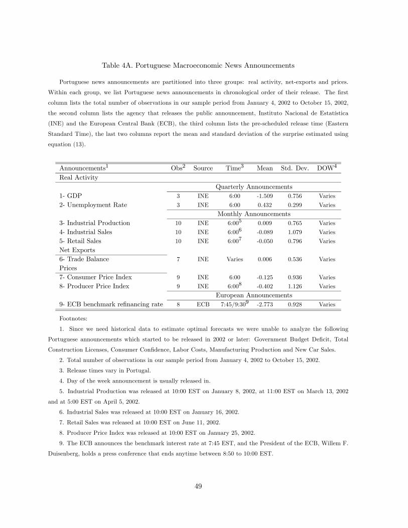
Table 4A. Portuguese Macroeconomic News Announcements

Portuguese news announcements are partitioned into three groups: real activity, net-exports and prices.

Within each group, we list Portuguese news announcements in chronological order of their release. The first

column lists the total number of observations in our sample period from January 4, 2002 to October 15, 2002,

the second column lists the agency that releases the public announcement, Instituto Nacional de Estatística

(INE) and the European Central Bank (ECB), the third column lists the pre-scheduled release time (Eastern

Standard Time), the last two columns report the mean and standard deviation of the surprise estimated using

equation (13).

Announcements1 Obs2 Source Time3 Mean Std. Dev. DOW4

Real ActivityQuarterly Announcements

1- GDP 3 INE 6:00 -1.509 0.756 Varies

2- Unemployment Rate 3 INE 6:00 0.432 0.299 Varies

Monthly Announcements3- Industrial Production 10 INE 6:005 0.009 0.765 Varies

4- Industrial Sales 10 INE 6:006 -0.089 1.079 Varies

5- Retail Sales 10 INE 6:007 -0.050 0.796 Varies

Net Exports6- Trade Balance 7 INE Varies 0.006 0.536 Varies

Prices7- Consumer Price Index 9 INE 6:00 -0.125 0.936 Varies

8- Producer Price Index 9 INE 6:008 -0.402 1.126 Varies

European Announcements9- ECB benchmark refinancing rate 8 ECB 7:45/9:309 -2.773 0.928 Varies

Footnotes:

1. Since we need historical data to estimate optimal forecasts we were unable to analyze the following

Portuguese announcements which started to be released in 2002 or later: Government Budget Deficit, Total

Construction Licenses, Consumer Confidence, Labor Costs, Manufacturing Production and New Car Sales.

2. Total number of observations in our sample period from January 4, 2002 to October 15, 2002.

3. Release times vary in Portugal.

4. Day of the week announcement is usually released in.

5. Industrial Production was released at 10:00 EST on January 8, 2002, at 11:00 EST on March 13, 2002

and at 5:00 EST on April 5, 2002.

6. Industrial Sales was released at 10:00 EST on January 16, 2002.

7. Retail Sales was released at 10:00 EST on June 11, 2002.

8. Producer Price Index was released at 10:00 EST on January 25, 2002.

9. The ECB announces the benchmark interest rate at 7:45 EST, and the President of the ECB, Willem F.

Duisenberg, holds a press conference that ends anytime between 8:50 to 10:00 EST.

49

Table 4B. U.S. Macroeconomic News Announcements

Announcements Obs1 Source2 Time3 Mean Std. Dev. DOW4

Real ActivityQuarterly Announcements

1- GDP Advance 3 BEA 8:30 0.342 1.649 Varies

2- GDP Preliminary 3 BEA 8:30 0.497 1.386 Varies

3- GDP Final 3 BEA 8:30 1.108 0.508 Varies

Monthly Announcements4- Nonfarm Payroll 10 BLS 8:30 -0.069 0.349 Friday5

5- Retail Sales 9 BC 8:30 0.143 0.975 Varies

6- Industrial Production 8 FRB 9:15 0.074 1.010 Varies

7- Capacity Utilization 8 FRB 9:15 0.175 0.856 Varies

8- Personal Income 8 BEA 8:30 0.049 0.680 Varies

9- Consumer Credit 9 FRB 15:00 0.352 2.174 Varies

Consumption10- New Home Sales 9 BC 10:00 0.262 1.038 Varies

11- Personal Consumption Expenditures 8 BEA 8:30 -0.146 0.669 Varies

Investment12- Durable Goods Orders 9 BC 8:30 0.284 1.020 Varies

13- Factory Orders 10 BC 10:00 -0.147 0.726 Varies

14- Construction Spending 7 BC 10:00 -0.188 1.081 Varies

15- Business Inventories 10 BC 8:30 0.171 0.886 Varies

Government Purchases16- Government Budget 9 FMS 14:00 -0.129 0.510 Varies

Net Exports17- Trade Balance 9 BEA 8:30 -0.168 1.118 Varies

Prices18- Producer Price Index 10 BLS 8:30 -0.546 1.076 Varies

19- Consumer Price Index 9 BLS 8:30 -0.377 0.768 Varies

Forward-Looking20- Consumer Confidence Index 9 CB 10:00 0.083 1.062 Tuesday6

21- NAPM Index 8 NAPM 10:00 0.113 1.330 Varies

22- Housing Starts 9 BC 8:30 0.103 0.572 Varies

23- Index of Leading Indicators 9 CB 8:30 0.302 1.126 Varies

Six-Week Announcements24- Target Federal Funds Rate 6 FRB 14:15 -0.525 0.605 Tuesday7

Weekly Announcements25- Initial Unemployment Claims 40 ETA 8:30 0.139 1.045 Thursday

50

Notes to Table 4B

U.S. news announcements are partitioned into seven groups: real activity, each of the GDP components

(consumption, investment, government purchases and net exports), prices, and forward-looking. Within each

group, we list U.S. news announcements in chronological order of their release. The last two columns list the

mean and standard deviation of the surprise estimated using equation (13).

Footnotes:

1. Total number of observations in our sample period from January 4, 2002 to October 15, 2002.

2. Bureau of Labor Statistics (BLS), Bureau of the Census (BC), Bureau of Economic Analysis (BEA),

Federal Reserve Board (FRB), National Association of Purchasing Managers (NAPM), Conference Board (CB),

Financial Management Office (FMO), Employment and Training Administration (ETA).

3. Eastern Standard Time. Daylight savings time starts on the first Sunday of April and ends on the last

Sunday of October.

4. Day of the week announcement is usually released in.

5. Nonfarm Payroll is released the first Friday of the month.

4. The Conference Board’s Consumer Confidence Index is released the last Tuesday of the month.

5. The FOMC has eight scheduled meetings per year. Since March 22, 1994 these meetings are usually

scheduled on Tuesday, except for the first meeting of the year, which is a two-day meeting starting on Tuesday

and ending on Wednesday when the announcement is released to the public.

51

Table 5. Aggregate Portuguese and U.S. Macroeconomic News Announcements

This table reports estimates of the aggregate Portuguese and U.S. News. We aggregate announcements into

seven groups as shown in Table 4A and Table 4B: real activity, each of the GDP components (i.e., consumption,

investment, government purchases and net exports), prices, and forward-looking announcements. The six-week

and weekly announcements are not aggregated. For example, U.S. real activity surprises are defined as the sum

of GDP Advance, GDP Preliminary, GDP Final, Nonfarm Payroll, Retail Sales, Industrial Production, Capacity

Utilization, Personal Income and Consumer Credit standardized surprises (according to equation (13)), while

Portuguese real activity surprises are defined as the sum of GDP, the Employment Report, Industrial Production

and Industrial Sales standardized surprises.

Announcements Obs Mean Std. Dev.Portuguese Announcements

1- Earnings 60 0.094 1.206

2- Real Activity 35 -0.127 0.939

3- Net Exports 7 0.006 0.536

4- Prices 18 -0.264 1.014

European Announcements5- ECB benchmark refinancing rate 8 -2.773 0.928

U.S. Announcements6- Earnings 83 0.891 1.345

7- Real Activity 55 0.257 1.254

8- Consumption 17 0.070 0.882

9- Investment 38 0.027 0.888

10- Government Purchases 9 -0.129 0.510

11- Net Exports 9 -0.168 1.118

12- Prices 19 -0.466 0.921

13- Forward-Looking 36 0.111 0.982

14- Target Federal Funds Rate 6 -0.525 0.605

15- Initial Unemployment Claims 40 0.139 1.045

52

Table 6. Influence of U.S. Macroeconomic Announcements on U.S. Returns

This table reports coefficient estimates of the following equation:

rusit = a+ λspeusSipeust+λspecbSpecbt+15X

pus=7

λspusSpust+JX

j=0

λjΩusit−j(1−Dus

t )+

JXj=0

λpjΩusit−jD

ust +

JXj=1

βjrusit−j(1−Dus

t )+JX

j=1

βpjrusit−jD

ust +εit,

where rusit is the daily stock return for i = 1, ..., 30 DJ 30 individual stocks, Ωusit is the unanticipated order flow (defined

in Section 6), Dust is an indicator function equal to one if a U.S. public announcement (earnings or macroeconomic news)

is released on date t, Sipeust is the standardized earnings news surprise for stock return i, Specbt is the standardized ECB

benchmark refinancing rate news surprise, and Spust is the aggregate standardized U.S. macroeconomic news surprise

for pus = 7, ..., 15 (defined in Section 4.2 and listed in Table 5). The t-statistics are estimated using the GARCH(1,1)-X

model (equation (19)) to correct for heteroskedasticity and autocorrelation. We mark the coefficients and F-statistics

with a “ ∗ ”, “ ∗∗ ”, or “ ∗∗∗ ” to indicate significance at the 10%, 5%, or 1% level, respectively.

Coefficient t-statisticContemporaneous Order Flow

Non-Announcement, λ0 0.0102 19.39∗∗∗

Announcement, λp0 0.0084 23.08∗∗∗

H0: λ0−λp0= 0 (F-statistic) 0.0018 8.59∗∗∗

Lagged Order FlowNon-Announcement, λ1 -0.0029 -5.11∗∗∗

Non-Announcement, λ2 -0.0010 -1.61

Announcement, λp1 -0.0016 -3.86∗∗∗

Announcement, λp2 -0.0011 -2.78∗∗∗

European Announcement, λspecbECB benchmark refinancing rate -0.1703 -3.44∗∗∗

U.S. Announcements, λspeus , λspusEarnings 0.5595 4.58∗∗∗

Real Activity 0.1680 3.38∗∗∗

Consumption 0.8889 7.85∗∗∗

Investment 0.1258 1.77∗

Government Purchases 0.0050 0.02

Net Exports 0.3678 3.46∗∗∗

Prices -0.1570 -1.86∗

Forward-Looking 0.2351 3.20∗∗∗

Target Federal Funds Rate -0.7300 -4.21∗∗∗

Initial Unemployment Claims -0.1010 -2.26∗∗

H0: λpors7 = ... = λpors15 = 0 (F-statistic) 13.42∗∗∗

Adjusted-R2 0.1665

53

Table 7. Influence of News Announcements on US-Portuguese Stock Market Comovement

Portuguese Portuguese U.S.Macroeconomic Ann. Earnings Ann. Macroeconomic Ann.

Contemporaneous Order FlowNon-Announcement, λpor0 0.0182∗∗∗ 0.0186∗∗∗ 0.0193∗∗∗ 0.0141∗∗∗ 0.0235∗∗∗ 0.0165∗∗∗

Announcement, λporp0 0.0240∗∗∗ 0.0244∗∗∗ 0.0097 0.0101∗ 0.0187∗∗∗ 0.0131∗∗∗

H0 : λpor0 − λporp0 = 0, (F-statistic) -0.0058∗∗∗ -0.0058∗∗∗ 0.0096 0.0039 0.0048∗∗ 0.0034∗∗∗

Lagged Order FlowNon-Announcement, λpor1 -0.0038∗∗∗ -0.0048∗∗∗ -0.0036∗∗∗ -0.0033∗∗∗ -0.0060∗∗ -0.0045∗∗∗

Non-Announcement, λpor2 -0.0027∗∗ -0.0020∗ -0.0023∗∗ -0.0015∗∗ -0.0050∗∗ -0.0016

Announcement, λporp1 -0.0051∗ -0.0044 -0.0025 -0.0034 -0.0036∗∗ -0.0033∗∗∗

Announcement, λporp2 -0.0012 -0.0001 -0.0050∗ -0.0022∗ -0.0013 -0.0013∗∗

U.S. Value Weighted ReturnNon-Announcement, βpor0 0.2515∗∗∗ 0.2289∗∗∗ 0.2278∗∗∗

Announcement, βpor0p 0.0867∗∗∗ 0.2367∗ 0.2370∗∗∗

H0 : βpor0 − βpor0p = 0, (F-statistic) 0.1648∗∗∗ -0.0078 -0.0092

Portuguese Announcements, λporspepor , λporsppor

Earnings 0.8201∗∗∗ 0.7349∗∗∗ 0.8411∗∗∗ 0.7701∗∗∗ 0.7741∗∗∗ 0.7558∗∗∗

Real Activity 0.0058 0.1546∗∗∗ 0.0217 0.2623∗∗∗ 0.0215 0.2443∗∗∗

Net Exports 0.5737∗∗∗ 0.4920∗∗∗ 0.5768∗∗∗ 0.4833∗∗∗ 0.6150∗∗∗ 0.4489∗∗∗

Prices -0.2975∗∗∗ -0.2289∗∗∗ -0.3013∗∗∗ -0.1515∗∗∗ -0.3108∗∗∗ -0.1417∗∗∗

H0: λpors2 = λpors3 = λpors4 = 0 (F-statistic) 10.53∗∗∗ 12.58∗∗∗ 11.32∗∗∗ 13.32∗∗∗ 12.82∗∗∗ 11.92∗∗∗

European Announcement, λporspecbECB benchmark refinancing rate -0.0910∗∗ -0.0163 -0.0685∗∗ -0.0560 -0.0765∗∗ -0.0539

U.S. Announcements, λporspusReal Activity 0.0399 -0.0292 0.0399 -0.0225 0.0411 -0.0219

Consumption 0.1967∗ -0.2320∗∗ 0.1935∗ -0.1863∗ 0.1940∗ -0.1827∗

Investment 0.1429∗ 0.0188 0.1372∗ 0.0232 0.1402∗ 0.0278

Government Purchases 0.3094 0.0499 0.2902 0.0457 0.2928 0.0549

Net Exports 0.0431 -0.1774 0.0516 -0.1355 0.0402 -0.1420

Prices -0.0578 0.1256 -0.0385 0.0948 -0.0369 0.0974

Forward-Looking 0.1615∗∗ 0.1132∗ 0.1655∗∗ 0.1331∗∗ 0.1647∗∗ 0.1317∗∗

Target Federal Funds Rate -1.3058∗∗∗ -0.8551∗∗∗ -1.3209∗∗∗ -0.8765∗∗∗ -1.3085∗∗∗ -0.8664∗∗∗

Initial Unemployment Claims -0.1216∗∗ -0.0300 -0.1248∗∗ -0.0429 -0.1177∗∗ -0.0383

H0: λpors7 = ... = λpors15 = 0 (F-statistic) 6.93∗∗∗ 3.30∗∗∗ 6.98∗∗∗ 3.12∗∗∗ 6.86∗∗∗ 3.07∗∗∗

Adjusted-R2 0.1652 0.2270 0.1670 0.2335 0.1621 0.2328

54

Notes to Table 7

This table reports coefficient estimates of the following equation:

rporit = apor+λporspeporSipeport + λporspecbSpecbt +

4Xppor=2

λporspporSpport+15X

pus=7

λporspusSpust+JX

j=0

λporj Ωporit−j(1−Dt)+

JXj=0

λporpj Ωporit−jDt+

JXj=0

βporj rust−j(1−Dt)+JX

j=0

βporpj rust−jDt+JXj=1

βporporjrporit−j+ε

porit ,

where rporit is the daily return for stock i = 1, ..., 20 of the PSI-20 Index, Ωporit is the daily Portuguese unantici-

pated order flow for stock i (defined in Section 6), Dt = Dport ,Depor

t ,Dust is an indicator function equal to one

if a Portuguese macroeconomic announcement, Portuguese earnings announcement, and a U.S. macroeconomic

annoucement is released, respectively, on date t , Specbt is the standardized ECB benchmark refinancing rate

news surprise, Sipeport is the Portuguese standardized earnings news surprise for stock i, and Spust is the aggre-

gate standardized U.S. macroeconomic news surprise for pus = 7, ..., 15 and Spport is the aggregate Portuguese

standardized macroeconomic news surprise for ppor = 2, 3, 4 (both of which are defined in Section 4.2 and listed

in Table 5). The coefficients in column one and two correspond to the equation estimates when Dt = Dport , the

coefficients in column three and four correspond to the equation estimates when Dt = Deport , and the coefficients

in the last two columns correspond to the equation estimates when Dt = Dust . The t-statistics are estimated

using the GARCH(1,1)-X model (equation (21)) to correct for heteroskedasticity and autocorrelation. We mark

the coefficients and F-statistics with a “ ∗ ”, “ ∗∗ ”, or “ ∗∗∗ ” to indicate significance at the 10%, 5%, or 1%

level, respectively.

55

Table 8. Influence of U.S. Disaggregate Macroeconomic Announcements on U.S. Returns

Coefficient t-statisticContemporaneous Order Flow

Non-Announcement, λ0 0.0105 20.65∗∗∗

Announcement, λp0 0.0084 22.25∗∗∗

H0 : λ0 − λp0 = 0 (F-statistic) 0.0021 11.18∗∗∗

European AnnouncementECB benchmark refinancing rate -0.1613 -2.92∗∗∗

U.S. AnnouncementsEarnings 0.4906 3.89∗∗∗

GDP Advance -0.5452 -3.71∗∗∗

GDP Preliminary -0.0370 -0.25

GDP Final 0.1142 0.47

Nonfarm Payroll 0.1573 0.32

Retail Sales -0.0227 -0.18

Industrial Production -0.1628 -0.48

Capacity Utilization 1.1817 3.67∗∗∗

Personal Income 1.2411 4.28∗∗∗

Consumer Credit 0.1778 2.01∗∗

New Home Sales -0.6252 -4.8∗∗∗

Personal Consumption Expenditures 1.9291 10.7∗∗∗

Durable Goods Orders 0.3076 2.51∗∗

Factory Orders 0.0839 0.64

Construction Spending 0.2049 0.57

Business Inventories -0.1039 -0.55

Government Budget 0.1917 0.88

Trade Balance 0.4005 3.61∗∗∗

Producer Price Index 0.0090 0.06

Consumer Price Index -0.1917 -1.33

Consumer Confidence Index 0.0064 0.06

NAPM Index -0.5410 -1.88∗

Housing Starts -1.1441 -6.17∗∗∗

Index of Leading Indicators 0.4112 3.48∗∗∗

Initial Unemployment Claims -0.1128 -2.56∗∗

Target Federal Funds Rate -0.9267 -4.73∗∗∗

Adjusted-R2 0.1763

56

Notes to Table 8

This table reports coefficient estimates of the following equation:

rusit = a+ λspeusSipeust+λspecbSpecbt+25X

pus=1

λspusSpust+JX

j=0

λjΩusit−j(1−Dus

t )+

JXj=0

λpjΩusit−jD

ust +

JXj=1

βjrusit−j(1−Dus

t )+JX

j=1

βpjrusit−jD

ust +εit,

where rusit is the daily stock return for i = 1, ..., 30 DJ 30 individual stocks, Ωusit is the daily U.S. unanticipated

order flow for stock i (defined in Section 6), Dust is an indicator function equal to one if a U.S. public announcement

(earnings or macroeconomic news) is released on date t, Sipeust is the standardized earnings news surprise for stock

return i, Specbt is the standardized ECB benchmark refinancing rate news surprise, and Spust is the disaggregate

standardized U.S. macroeconomic news surprise for pus = 1, ..., 25 (defined in Section 4.2 and listed in Table 4B).

The t-statistics are estimated using the GARCH(1,1)-X model (equation (19)) to correct for heteroskedasticity

and autocorrelation. We mark the coefficients and F-statistics with a “ ∗ ”, “ ∗∗ ”, or “ ∗∗∗ ” to indicate

significance at the 10%, 5%, or 1% level, respectively.

57

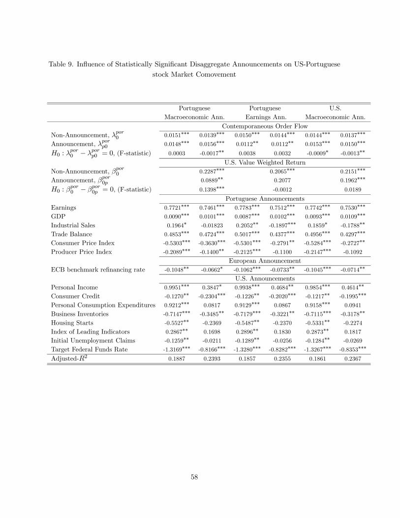
Table 9. Influence of Statistically Significant Disaggregate Announcements on US-Portuguesestock Market Comovement

Portuguese Portuguese U.S.Macroeconomic Ann. Earnings Ann. Macroeconomic Ann.

Contemporaneous Order FlowNon-Announcement, λpor0 0.0151∗∗∗ 0.0139∗∗∗ 0.0150∗∗∗ 0.0144∗∗∗ 0.0144∗∗∗ 0.0137∗∗∗

Announcement, λporp0 0.0148∗∗∗ 0.0156∗∗∗ 0.0112∗∗ 0.0112∗∗ 0.0153∗∗∗ 0.0150∗∗∗

H0 : λpor0 − λporp0 = 0, (F-statistic) 0.0003 -0.0017∗∗ 0.0038 0.0032 -0.0009∗ -0.0013∗∗

U.S. Value Weighted ReturnNon-Announcement, βpor0 0.2287∗∗∗ 0.2065∗∗∗ 0.2151∗∗∗

Announcement, βpor0p 0.0889∗∗ 0.2077 0.1962∗∗∗

H0 : βpor0 − βpor0p = 0, (F-statistic) 0.1398∗∗∗ -0.0012 0.0189

Portuguese AnnouncementsEarnings 0.7721∗∗∗ 0.7461∗∗∗ 0.7783∗∗∗ 0.7512∗∗∗ 0.7742∗∗∗ 0.7530∗∗∗

GDP 0.0090∗∗∗ 0.0101∗∗∗ 0.0087∗∗∗ 0.0102∗∗∗ 0.0093∗∗∗ 0.0109∗∗∗

Industrial Sales 0.1964∗ -0.01823 0.2052∗∗ -0.1897∗∗∗ 0.1859∗ -0.1788∗∗

Trade Balance 0.4853∗∗∗ 0.4724∗∗∗ 0.5017∗∗∗ 0.4377∗∗∗ 0.4956∗∗∗ 0.4297∗∗∗

Consumer Price Index -0.5303∗∗∗ -0.3630∗∗∗ -0.5301∗∗∗ -0.2791∗∗ -0.5284∗∗∗ -0.2727∗∗

Producer Price Index -0.2089∗∗∗ -0.1400∗∗ -0.2125∗∗∗ -0.1100 -0.2147∗∗∗ -0.1092

European AnnouncementECB benchmark refinancing rate -0.1048∗∗ -0.0662∗ -0.1062∗∗∗ -0.0733∗∗ -0.1045∗∗∗ -0.0714∗∗

U.S. AnnouncementsPersonal Income 0.9951∗∗∗ 0.3847∗ 0.9938∗∗∗ 0.4684∗∗ 0.9854∗∗∗ 0.4614∗∗

Consumer Credit -0.1270∗∗ -0.2304∗∗∗ -0.1226∗∗ -0.2020∗∗∗ -0.1217∗∗ -0.1995∗∗∗

Personal Consumption Expenditures 0.9212∗∗∗ 0.0817 0.9129∗∗∗ 0.0867 0.9158∗∗∗ 0.0941

Business Inventories -0.7147∗∗∗ -0.3485∗∗ -0.7179∗∗∗ -0.3221∗∗ -0.7115∗∗∗ -0.3178∗∗

Housing Starts -0.5527∗∗ -0.2369 -0.5487∗∗ -0.2370 -0.5331∗∗ -0.2274

Index of Leading Indicators 0.2867∗∗ 0.1698 0.2896∗∗ 0.1830 0.2873∗∗ 0.1817

Initial Unemployment Claims -0.1259∗∗ -0.0211 -0.1289∗∗ -0.0256 -0.1284∗∗ -0.0269

Target Federal Funds Rate -1.3169∗∗∗ -0.8166∗∗∗ -1.3280∗∗∗ -0.8282∗∗∗ -1.3267∗∗∗ -0.8353∗∗∗

Adjusted-R2 0.1887 0.2393 0.1857 0.2355 0.1861 0.2367

58

Notes to Table 9

This table reports coefficient estimates of the following equation:

rporit = apor+λporspeporSipeport + λporspecbSpecbt +

PporXppor=1

λporspporSpport+PusX

pus=1

λporspusSpust+JX

j=0

λporj Ωporit−j(1−Dt)+

JXj=0

λporpj Ωporit−jDt+

JXj=0

βporj rust−j(1−Dt)+JX

j=0

βporpj rust−jDt+JXj=1

βporporjrporit−j+ε

porit ,

where rporit is the daily return for stock i = 1, ..., 20 of the PSI-20 Index, Ωporit is the daily Portuguese unanticipated

order flow for stock i (defined in Section 6), Dt = Dport ,Depor

t ,Dust is an indicator function equal to one if

a statistically significant Portuguese macroeconomic announcement, Portuguese earnings announcement, and a

statistically significant U.S. macroeconomic annoucement is released, respectively, on date t , Specbt is the stan-

dardized ECB benchmark refinancing rate news surprise, Sipeport is the Portuguese standardized earnings news

surprise for stock i, and Spust is the disaggregate standardized U.S. macroeconomic news surprise for statistically

significant news pus = 1, ...,Pus and Spport is the disaggregate Portuguese standardized macroeconomic news

surprise for statistically significant news ppor = 1, ...,Ppor. The coefficients in column one and two correspond

to the equation estimates when Dt = Dport , the coefficients in column three and four correspond to the equation

estimates when Dt = Deport , and the coefficients in the last two columns correspond to the equation estimates

when Dt = Dust . The t-statistics are estimated using the GARCH(1,1)-X model (equation (21)) to correct for

heteroskedasticity and autocorrelation. We mark the coefficients and F-statistics with a “ ∗ ”, “ ∗∗ ”, or “ ∗∗∗ ”

to indicate significance at the 10%, 5%, or 1% level, respectively.

59

Table 10. Day of the Week Effects and Large U.S. Returns

Coefficient t-statistic Coefficient t-statisticContemporaneous Order Flow

λpor0 0.0136 43.45∗∗∗ 0.0134 40.90∗∗∗

Lagged Order Flowλpor1 -0.0032 -6.70∗∗∗ -0.0030 -5.83∗∗∗

λpor2 -0.0016 -3.24∗∗∗ -0.0014 -2.58∗∗∗

λpor3 -0.0014 -2.62∗∗∗ -0.0016 -2.65∗∗∗

U.S. Value Weighted Returnβpor0 0.2200 10.58∗∗∗ 0.2551 10.44∗∗∗

βpor0LARGE 0.0251 0.99

Monday, βpor0 0.0114 0.30

Tuesday, βpor0 -0.0413 -1.11

Wednesday, βpor0 -0.0170 -0.37

Thursday, βpor0 -0.0647 -1.72∗

Portuguese Announcements, λpore , λporsp

Earnings 0.7457 5.92∗∗∗ 0.7920 7.06∗∗∗

Real Activity 0.2277 4.05∗∗∗ 0.2156 4.17∗∗∗

Net Exports 0.4785 3.87∗∗∗ 0.4859 2.63∗∗∗

Prices -0.1799 -3.26∗∗∗ -0.1258 -2.23∗∗

F-statistic 10.12∗∗∗ 13.43∗∗∗

European Announcement, λusecbECB benchmark refinancing rate -0.0578 -1.72∗ -0.0503 -1.37

U.S. Announcements, λporsp

Real Activity -0.0117 -0.3 -0.0214 -0.54

Consumption -0.1953 -1.81∗ -0.1780 -1.56

Investment 0.0334 0.47 0.0307 0.43

Government Purchases 0.1057 0.41 0.0500 0.19

Net Exports -0.1132 -0.97 -0.1520 -1.26

Prices 0.0803 0.93 0.0869 0.99

Forward-Looking 0.1383 2.07∗∗ 0.1254 1.87∗

Target Federal Funds Rate -0.8698 -4.26∗∗∗ -0.8777 -4.24∗∗∗

Initial Unemployment Claims -0.0350 -0.62 -0.0409 -0.71

F-statistic 2.62∗∗∗ 2.60∗∗∗

Adjusted-R2 0.2334 0.2321

60

Notes to Table 10

This table reports coefficient estimates of the following equation:

rporit = apor+λporspeporSipeport + λporspecbSpecbt +

PporXppor=1

λporspporSpport+PusX

pus=1

λporspusSpust+JX

j=0

λporj Ωporit−j(1−Dt)+

JXj=0

λporpj Ωporit−jDt+

JXj=0

βporj rust−j(1−Dt)+JX

j=0

βporpj rust−jDt+JXj=1

βporporjrporit−j+ε

porit ,

where rporit is the daily return for stock i = 1, ..., 20 of the PSI-20 Index, Ωporit is the daily Portuguese unanticipated

order flow for stock i (defined in Section 6), Dt = DLARGEt , DMonday

t ,DTuesdayt , DWednesday

t ,DThrusdayt

where DLARGEt is an indicator function equal to one if the U.S. value weighted DJ 30 index experiences a top

10% jump on day t, and DMondayt , DTuesday

t ,DWednesdayt ,DThrusday

t are day-of-the week indicator functions,

Specbt is the standardized ECB benchmark refinancing rate news surprise, Sipeport is the Portuguese standardized

earnings news surprise for stock i, and Spust is the aggregate standardized U.S. macroeconomic news surprise

pus = 2, ...,7 and Spport is the aggregate Portuguese standardized macroeconomic news surprise ppor = 2, 3, 4.

The t-statistics are estimated using the GARCH(1,1)-X model (equation (21)) to correct for heteroskedasticity

and autocorrelation. We mark the coefficients and F-statistics with a “ ∗ ”, “ ∗∗ ”, or “ ∗∗∗ ” to indicate

significance at the 10%, 5%, or 1% level, respectively

61

Figure 1. Timeline of Events

Foreign Economy Local Economy

Market makers observe

Public news U∗t arrives, aggregate order flow Public news Ut and P∗t arrives, Market makers observe

t informed traders learn s∗t ω∗t =Pn

i=1 x∗it + z∗t informed traders learn st ωt =

Pni=1 xit + zt t+ 1

←→ ←→Orders are placed: x∗it, z

∗t Price is chosen P ∗t . Orders are placed: xit, zt Price is chosen Pt.

62

Figure 2A. Portugues Response to 7:45 ECB announcement, 8:30 and 9:15 EST U.S.Macroeconomic Announcements

We plot λporsp (equation (16)), the cumulative Portuguese response to 8:30 and 9:15 EST U.S. macroeconomic

announcements, and the 7:45 EST ECB announcement. The left hand side of the x-axis in each plot coincides

with the time indicated in the title of the plot. Each tick advances time by 5 minutes. For example, in the top

left hand corner plot the first tick indicates 7:50 EST and the return is measured from just before 7:45 EST to

7:50 EST. The second tick indicates 7:55 EST and the return is measured from just before 7:45 EST to 7:55

EST. The vertical line corresponds to 9:30 EST when the U.S. stock market opens. The last tick captures the

response from the time indicated in the title of the plot to 11:30 EST.

-0.4

-0.2

0.0

0.2

0.4

5 10 15 20 25 30 35 40 45

Res

pons

e

Time

ECB Benchmark Rate 7:45

-0.4

-0.2

0.0

0.2

0.4

5 10 15 20 25 30 35

Res

pons

e

Time

Real Activity 8:30

-0.4

-0.2

0.0

0.2

0.4

5 10 15 20 25 30 35R

espo

nse

Time

Consumption 8:30

-0.4

-0.2

0.0

0.2

0.4

5 10 15 20 25 30 35

Res

pons

e

Time

Investment 8:30

-0.4

-0.2

0.0

0.2

0.4

5 10 15 20 25 30 35

Res

pons

e

Time

Net Exports 8:30

-0.4

-0.2

0.0

0.2

0.4

5 10 15 20 25 30 35

Res

pons

e

Time

Prices 8:30

-0.4

-0.2

0.0

0.2

0.4

5 10 15 20 25 30 35

Res

pons

e

Time

Forward-Looking 8:30

-0.4

-0.2

0.0

0.2

0.4

5 10 15 20 25 30 35

Res

pons

e

Time

Initial Unemployment Claims 8:30

-0.4

-0.2

0.0

0.2

0.4

5 10 15 20 25

Res

pons

e

Time

Real Activity 9:15

63

Figure 2B. U.S. Response to 7:45 ECB announcement, 8:30 and 9:15 EST U.S.Macroeconomic Announcements

We plot λsp (equation (16)), the cumulative U.S. response to 8:30 and 9:15 EST U.S. macroeconomic

announcements, and the 7:45 EST ECB announcement. Since the U.S. stock market is not yet open, the first

tick in all panels on the x-axis captures the U.S. stock market response from the previous day’s close to 9:35

EST, the second tick captures the cumulative response from the previous day’s close to 9:40 EST, and so on.

The last tick captures the response from the previous day’s close to 11:30 EST.

-0.8-0.6-0.4-0.20.00.20.40.60.8

5 10 15 20

Res

pons

e

Time

ECB Benchmark Rate 7:45

-0.8-0.6-0.4-0.20.00.20.40.60.8

5 10 15 20

Res

pons

e

Time

Real Activity 8:30

-0.5

0.0

0.5

1.0

1.5

2.0

5 10 15 20

Res

pons

eTime

Consumption 8:30

-0.8-0.6-0.4-0.20.00.20.40.60.8

5 10 15 20

Res

pons

e

Time

Investment 8:30

-0.8-0.6-0.4-0.20.00.20.40.60.8

5 10 15 20

Res

pons

e

Time

Net Exports 8:30

-0.8-0.6-0.4-0.20.00.20.40.60.8

5 10 15 20

Res

pons

e

Time

Prices 8:30

-0.8-0.6-0.4-0.20.00.20.40.60.8

5 10 15 20

Res

pons

e

Time

Forward-Looking 8:30

-0.8-0.6-0.4-0.20.00.20.40.60.8

5 10 15 20

Res

pons

e

Time

Initial Unemployment Claims 8:30

-0.8-0.6-0.4-0.20.00.20.40.60.8

5 10 15 20

Res

pons

e

Time

Real Activity 9:15

64

Figure 3A. Portuguese Response to 10:00 EST U.S. Macroeconomic Announcements

We plot λporsp (equation (16)), the cumulative Portuguese response to 10:00 EST U.S. macroeconomic an-

nouncements. The first tick in all panels on the x-axis captures the U.S. stock market response from 10:00 to

10:05 EST, the second tick captures the cumulative response from 10:00 to 10:10 EST, and so on. The last tick

captures the response from 10:00 to 11:30 EST.

-0.2

-0.1

0.0

0.1

0.2

0.3

0.4

0.5

2 4 6 8 10 12 14 16 18

Res

pons

e

Time

Consumption 10:00

-0.2

-0.1

0.0

0.1

0.2

0.3

0.4

0.5

2 4 6 8 10 12 14 16 18

Res

pons

e

Time

Investment 10:00

-0.05

0.00

0.05

0.10

0.15

2 4 6 8 10 12 14 16 18

Res

pons

e

Time

Forward-Looking 10:00

65

Figure 3B. U.S. Response to 10:00 EST U.S. Macroeconomic Announcements

We plot λsp (equation (16)), the cumulative U.S. response to 10:00 EST U.S. macroeconomic announcements.

The first tick in all panels on the x-axis captures the U.S. stock market response from 10:00 to 10:05 EST, the

second tick captures the cumulative response from 10:00 to 10:10 EST, and so on. The last tick captures the

response from 10:00 to 11:30 EST.

-0.2

-0.1

0.0

0.1

0.2

0.3

0.4

0.5

2 4 6 8 10 12 14 16 18

Res

pons

e

Time

Consumption 10:00

-0.2

-0.1

0.0

0.1

0.2

0.3

0.4

0.5

2 4 6 8 10 12 14 16 18

Res

pons

e

Time

Investment 10:00

-0.2

-0.1

0.0

0.1

0.2

0.3

0.4

0.5

2 4 6 8 10 12 14 16 18

Res

pons

e

Time

Forward-Looking 10:00

66

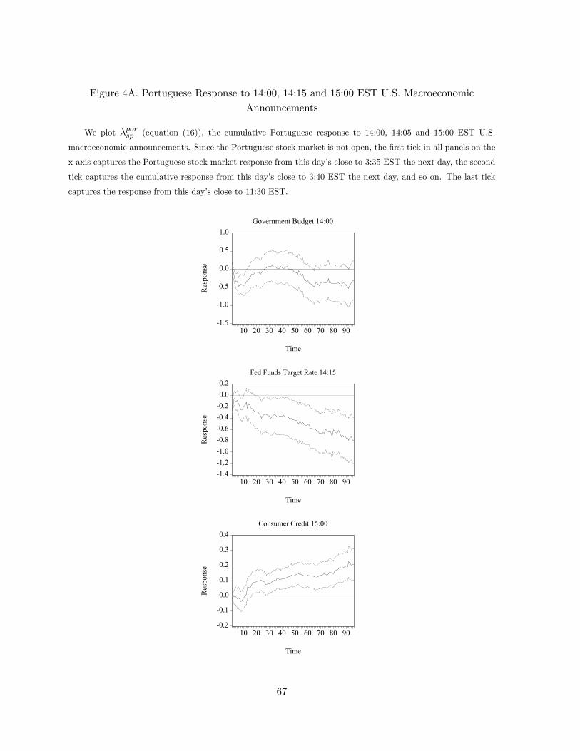
Figure 4A. Portuguese Response to 14:00, 14:15 and 15:00 EST U.S. MacroeconomicAnnouncements

We plot λporsp (equation (16)), the cumulative Portuguese response to 14:00, 14:05 and 15:00 EST U.S.

macroeconomic announcements. Since the Portuguese stock market is not open, the first tick in all panels on the

x-axis captures the Portuguese stock market response from this day’s close to 3:35 EST the next day, the second

tick captures the cumulative response from this day’s close to 3:40 EST the next day, and so on. The last tick

captures the response from this day’s close to 11:30 EST.

-1.5

-1.0

-0.5

0.0

0.5

1.0

10 20 30 40 50 60 70 80 90

Res

pons

e

Time

Government Budget 14:00

-1.4-1.2-1.0-0.8-0.6-0.4-0.20.00.2

10 20 30 40 50 60 70 80 90

Res

pons

e

Time

Fed Funds Target Rate 14:15

-0.2

-0.1

0.0

0.1

0.2

0.3

0.4

10 20 30 40 50 60 70 80 90

Res

pons

e

Time

Consumer Credit 15:00

67

Figure 4B. U.S. Response to 14:00, 14:15 and 15:00 EST U.S. Macroeconomic Announcements

We plot λsp (equation (16)), the cumulative U.S. response to 14:00, 14:15 and 15:00 EST U.S. macroeconomic

announcements. The left hand side of the x-axis in each plot coincides with the time indicated in the title of

the plot. Each tick advances time by 5 minutes. For example, in the top plot the first tick indicates 14:00 EST

and the return is measured from just before 14:00 EST to 14:05 EST. The second tick indicates 14:10 EST and

the return is measured from just before 14:00 EST to 14:10 EST, and so on. The last tick captures the response

from the time indicated in the title of the plot to 11:30 EST.

-1.5

-1.0

-0.5

0.0

0.5

1.0

5 10 15 20 25 30 35 40 45

Res

pons

e

Time

Government Budget 14:00

-4

-3

-2

-1

0

1

5 10 15 20 25 30 35 40 45

Res

pons

e

Time

Fed Funds Target Rate 14:15

-0.2

-0.1

0.0

0.1

0.2

0.3

0.4

5 10 15 20 25 30 35

Res

pons

e

Time

Consumer Credit 15:00

68