Asymmetry of information flow between volatilities across ...rgencay/jarticles/qf-hmm.pdf · Asymmetry of information flow between volatilities across time ... model regimes of volatilities

Quantitative Finance, Vol. 10, No. 8, October 2010, 895–915

Asymmetry of information flow between volatilities

across time scales

RAMAZAN GENCAY*y, NIKOLA GRADOJEVICz, FARUK SELCUKxk andBRANDON WHITCHER{

yDepartment of Economics, Simon Fraser University, 8888 University Drive, Burnaby,British Columbia V5A 1S6, Canada

zFaculty of Business Administration, Lakehead University, 955 Oliver Road,Thunder Bay, ON P7B 5E1, Canada

xDepartment of Economics, Bilkent University, Bilkent, Ankara 06533, Turkey{GlaxoSmithKline Clinical Imaging Centre, Hammersmith Hospital, London, UK

(Received 30 July 2007; in final form 29 October 2009)

Conventional time series analysis, focusing exclusively on a time series at a given scale, lacksthe ability to explain the nature of the data-generating process. A process equation thatsuccessfully explains daily price changes, for example, is unable to characterize the nature ofhourly price changes. On the other hand, statistical properties of monthly price changes areoften not fully covered by a model based on daily price changes. In this paper, wesimultaneously model regimes of volatilities at multiple time scales through wavelet-domainhidden Markov models. We establish an important stylized property of volatility acrossdifferent time scales. We call this property asymmetric vertical dependence. It is asymmetric inthe sense that a low volatility state (regime) at a long time horizon is most likely followed bylow volatility states at shorter time horizons. On the other hand, a high volatility state at longtime horizons does not necessarily imply a high volatility state at shorter time horizons. Ouranalysis provides evidence that volatility is a mixture of high and low volatility regimes,resulting in a distribution that is non-Gaussian. This result has important implicationsregarding the scaling behavior of volatility, and, consequently, the calculation of risk atdifferent time scales.

Keywords: Advanced econometrics; Anomalies in prices; Applied econometrics;Applied finance

1. Introduction

The fundamental properties of volatility dynamics are

volatility clustering (conditional heteroscedasticity) and

long memory (slowly decaying autocorrelation). Both

properties might be labeled as horizontal dependency when

viewing volatility in the time domain.$ In this paper, we

establish a third important stylized property of volatility

from a time-frequency point of view—the asymmetric

dependence of volatility across different time horizons.

Specifically, low volatility at a long time horizon is most

likely followed by low volatility at shorter time horizons.

On the other hand, high volatility at long time horizons

does not necessarily imply a high volatility at shorter time

horizons. We call this property asymmetric vertical

dependence.The motivation behind the vertical dependence in

volatility is the existence of traders with different time

horizons. At the outer layer of the trading mechanism are

the fundamentalist traders who trade on longer time

horizons. At lower layers, there are short-term traders

with a time horizon of a few days and day traders who*Corresponding author. Email: [email protected]

kDr. Selcuk passed away after this manuscript had been completed.$Clustering and long memory properties were first noted by Mandelbrot (1963, 1971). These findings remained dormant until Engle(1982) and Bollerslev (1986) proposed the ARCH and GARCH processes for volatility clustering. In the early 1990s, acomprehensive study of the long-memory properties of financial time series began.

Quantitative FinanceISSN 1469–7688 print/ISSN 1469–7696 online � 2010 Taylor & Francis

http://www.informaworld.comDOI: 10.1080/14697680903460143

Downloaded By: [Gencay, Ramazan] At: 05:36 15 September 2010

may carry positions only overnight. At the next level

down are the intraday traders who carry out trades only

during the day but do not carry overnight positions. At

the heart of trading mechanisms are the market makers

operating at the shortest time horizon (highest fre-

quency). Each of these types of traders may have their

own trading tools consistent with their trading horizon

and may possess a homogeneous appearance within their

own class. Overall, it is the combination of these activities

for all time scales that generates market prices. Therefore,

market activity would not exhibit homogeneous behavior,

but the underlying dynamics would be heterogeneous

with each trading class at each time scale dynamically

interacting across all trading classes at different time

scales.y In such a heterogeneous market, a low-frequency

shock to the system penetrates through all layers of

the entire market reaching the market makers. The

high-frequency shocks, however, would be short lived

and may have no impact outside their boundaries.Short-term traders constantly watch the market to

re-evaluate their current positions and execute transac-

tions at a high frequency. Long-term traders may look

at the market only once a day or less frequently. A

quick price increase followed by a quick decrease of the

same size, for example, is a major event for an intraday

trader but a non-event for central banks and long-term

investors.z Long-term traders are interested only in

large price movements and these normally happen only

over long time intervals. Therefore, long-term traders

with open positions have no need to watch the market

at every instance.x In other words, they judge the

market, its prices, and also its volatility with a coarse

time grid. A coarse time grid reflects the view of a

long-term trader and a fine time grid that of a

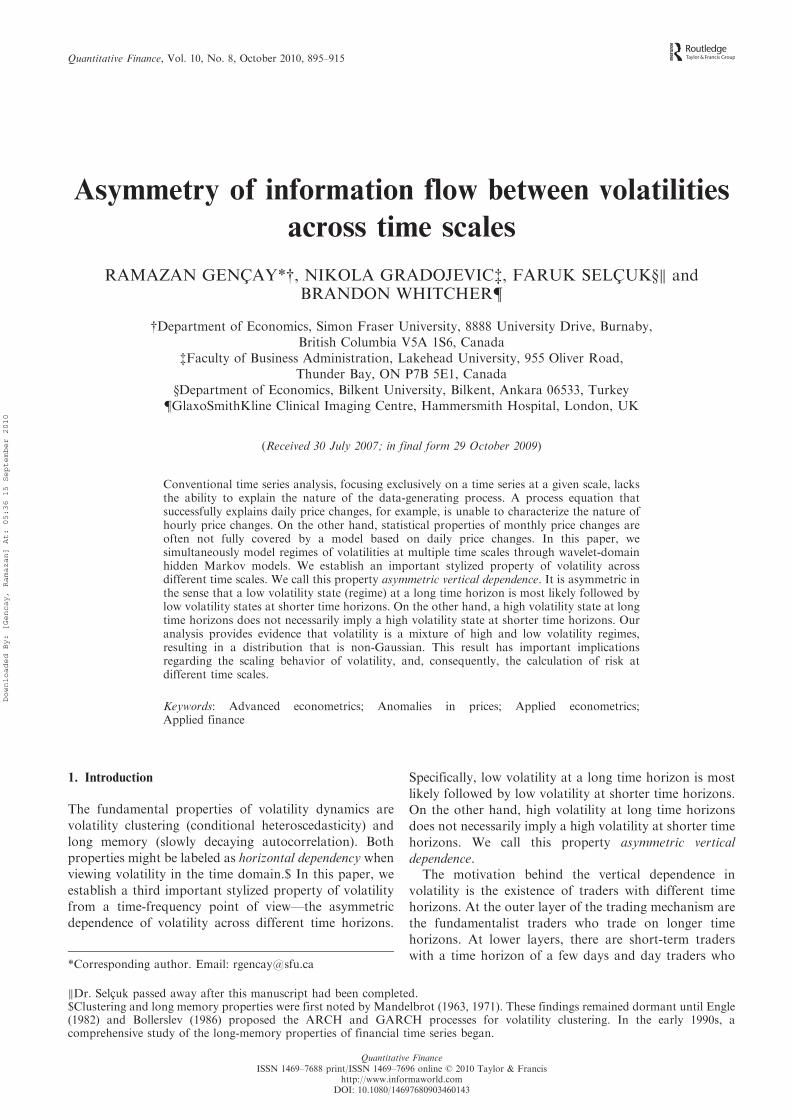
short-term trader.To explore the behavior of volatilities of different time

resolutions, Dacorogna et al. (2001) defined two types of

volatility, the ‘coarse’ volatility, vc, and the ‘fine’ volatil-

ity, vf, as illustrated in figure 1. The coarse volatility, vc(t),

captures the view and actions of long-term traders while

the fine volatility, vf(t), captures the view and actions of

short-term traders.�

It has been shown by Muller et al. (1997) and

Dacorogna et al. (2001) that there is asymmetry where

the coarse volatility predicts fine volatility better than the

other way around.? These findings have been confirmed

by Zumbach (2007) and discussed by Borland et al.

(2008).k In a related paper, Calvet and Fisher (2002)

capture volatility persistence across time scales and long

memory using the multifractal model of asset returns. The

analysis of high-frequency foreign exchange and stock

markets reveals volatility clustering at all time scales, as

well as evidence of multifractality in the moment-scaling

behavior of the data. In the same vein, Ghysels et al.

(2006) study the predictability of return volatility at

different frequencies by employing mixed data sampling

regressions. Their main findings suggest that absolute

returns are more successful predictors of future return

volatility than squared returns. More recently, Weber

et al. (2007) show that the memory in the volatility is

related to the Omori processes present on different time

scales.One of the goals of this paper is to investigate the

propagation properties of this heterogeneity-driven asym-

metry by studying the statistical properties of the flow

of information from low- to high-frequency scales.$

Low-frequency scales (fundamentalist-type traders)

are associated with traders who trade infrequently.

Figure 1. The coarse volatility, vc(t), captures the view andactions of long-term traders while the fine volatility, vf (t),captures the view and actions of short-term traders. The twovolatilities are calculated at the same time points where returns(rj) are measured and are synchronized.

yThe term ‘time scale’ may be viewed as a ‘resolution’. At high time scales (low frequencies, long term) there is a coarse resolution ofa time series, while at low time scales (high frequency, short term), there exists a high resolution. Moving from low time scales tohigh time scales (from short term to long term) leads to a more coarse characterization of the time series due to averaging.zSmall, short-term price moves may sometimes have a certain influence on the timing of long-term traders’ transactions but not ontheir investment decisions.xThey have other means to limit the risk of rare large price movements by stop-loss limits or options.�The two volatilities are calculated at the same time points where returns (rj) are measured and are synchronized.?The HARCH model of Muller et al. (1997) belongs to the ARCH family but differs from ARCH-type processes in a unique way ofconsidering the volatilities of returns measured over different interval sizes. The HARCH model has the ability to capture theasymmetry in the interaction between volatilities measured at different frequencies such that a coarsely defined volatility predicts afine volatility better than the other way around.kNotable contributions also include Zumbach and Lynch (2001) and Zumbach (2004). The present paper complements and extendsthis literature by investigating the link between both high and low volatilities across time scales. We not only provide evidence of‘vertical dependence’ in volatility, but also differentiate between the multiscale effects related to high and low volatilities.$The flow of dependence, from lower resolution (low-frequency content) to higher resolution (higher-frequency content) can berelaxed such that an analysis from higher-frequency to low-frequency content can be allowed. Durand and Goncalves (2001)comment that the directions of the directed acyclic graph (DAG) for the model of Crouse et al. (1998) is not necessary according to apaper by Smyth et al. (1996). In this paper, one can drop all directions in the graph and the conditional independence statementswould still be valid.

896 R. Gencay et al.


Therefore, the framework that we study focuses on the

impact of the actions of the long-term traders on

short-term traders who trade more frequently. Once theregime structure (state) is identified from low to high

frequency, this has implications for the flow of informa-

tion across time scales. In particular, a high-volatility

regime persists longer at longer (lower-frequency) trading

horizons relative to short (high-frequency) horizons.

Alternatively, the duration of regimes tends to be longerfor low-frequency trading horizons, whereas

high-frequency horizons have short-lived regime dura-

tions with frequent regime switching. This is not surpris-

ing since the impact of a change in long-term dynamics

would be short lived at higher frequencies.yIndeed, our findings indicate that a low volatility at a

low frequency implies a low volatility at higher frequen-cies. For example, if a low volatility is observed at a

weekly scale, it is more likely that there is also a low

volatility at a one day scale. However, a high volatility

at a low frequency does not necessarily imply a high

volatility at higher frequencies. This is because the market

‘calms down’ at higher frequencies much earlier than it

does at lower frequencies.Our modeling framework is based on wavelet-domain

hidden Markov models (HMMs). The wavelet HMMs are

distinct from traditional HMMs already used in time

series analysis.z Traditional HMMs capture the temporal

dependence within a given time scale, whereas wavelet

HMMs capture dependencies in the two-dimensional

time-frequency plane. In our analysis, we classifyhigh-frequency data into time horizons (scales) that are

consistent with the time scales in which traders operate.

Each time scale is characterized with a two-state regime of

high and low volatility. By connecting the state variables

vertically across scales, we obtain a graph with

tree-structured dependencies between state variablesacross different time scales. An implication of our

findings is that composition of states across adjacent

scales varies in time. Hence, simple aggregation of a daily

volatility to obtain a monthly volatility, for instance, may

not necessarily follow linear aggregation but may involve

nonlinearities through state switching.A simple way to think about wavelet multiscale analysis

is the following example: The day ends and one makes the

analysis of the day at various time intervals. For instance,

a trader may argue that the day overall was quiet with

minimal volatility except that there was high volatility

within a 10-min window in the morning trading around

10:00 a.m. Such a statement requires the trader to observe

the entire day and make references to specific time

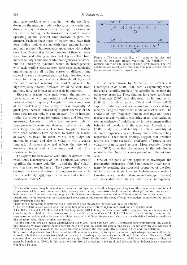
intervals in that trading day. Figure 2 illustrates this point

with an example from the New York Stock Exchange.

On January 3, 2001, the Dow Jones Industrial Average

(DJIA) increased from 10,646 (previous day closing

value) to 10,946 (closing value that day). The 2.82%

daily increase was relatively large and the market on this

day can be classified as ‘volatile’. However, a closer

inspection of 5-min DJIA values shows that the market

was not volatile during the entire trading session in that

day. If we look at the data from an hourly scale, the high

volatility took place at the beginning of the trading

session (first hour) and between 1:00 and 2:00 p.m. Other

than these two hours, the market was not volatile on an

hourly scale. Similarly, high volatility was only present for

certain intervals of the intraday scales this particular day.

A successful method to describe the market dynamics at

different scales (monthly, daily, hourly, etc.) must be able

to separate each time-scale component from the observed

data.x Although it is not common in economics and

finance, wavelet methodology has been proved to be

an excellent tool to reach this goal in several

scientific areas.

09:35 11:35 01:35 03:35−0.5

0

0.5

1

1.5

2

2.5

3

Jan−03−2001, 5−Min Intervals

DJI

A v

olat

ility

(ab

solu

te lo

g re

turn

), p

erce

nt

Figure 2. The Dow Jones Industrial Average (DJIA) volatilityduring January 3, 2001. On this day, the DJIA increased from10,646 (previous day closing value) to 10,946 (closing value thatday). The 2.82% daily increase was relatively large and themarket on this day can be classified as ‘volatile’. However, aclose inspection of 5-min DJIA values shows that the marketwas not volatile during the entire trading session.

yGencay et al. (2002, 2003) indicate that the foreign exchange returns may possess a multi-frequency conditional mean andconditional heteroskedasticity. The traditional heteroskedastic models fail to capture the entire dynamics by only capturing a slice ofthis dynamics at a given frequency. Therefore, a more realistic processes for foreign exchange returns should give consideration tothe scaling behavior of returns at different frequencies.zIn the economics and finance literature, the persistence of mean and volatility dynamics and nonlinearities through regimeswitching at a given data frequency (horizontal persistence) have been examined extensively within the context of Markov switchingmodels. The introduction of Markov switching models to the economics and finance literature is due to Hamilton (1989). Maheuand McCurdy (2002) is a recent study of high-frequency volatility using a Markov switching model.xOne apparent question regarding the wavelet methodology is whether comparisons of volatilities are fair, and whether there is anissue of the use of future information, as low-frequency volatility uses more information on the time-domain relative tohigh-frequency volatility. The usage of future information is not a concern, purely because of the fact that this study is an historicalanalysis describing market dynamics at different scales.

Asymmetry of information flow between volatilities 897


Wavelet coefficients decompose the information fromthe original time series into pieces associated with bothtime and scales. Since the wavelet coefficients capture thevariation of volatility at a given scale and interval of time,we model the wavelet coefficients directly. The waveletcoefficients can be viewed as differences between weightedaverages where the weights are determined by a givenwavelet filter. If the concern is the total variation of thedata at various time scales, it is essential to work withwavelet coefficients. For the current analysis, the impor-tant issue in a given scale is ‘how large a waveletcoefficient is’. If it is relatively large (relative to theaverage in this time scale), then it implies there was asudden change in average volatility at that scale, meaningthe system had switched to a ‘high-volatility state’. On theother hand, if the wavelet coefficient is small, it implies nolarge change in volatility (relative to the average in thattime scale) and that a ‘low-volatility state’ prevails.y

The outline of this paper is as follows. Section 2introduces the discrete wavelet transform in terms oforthonormal matrices and digital filters. Multiresolutionanalysis, the additive decomposition of a time series basedon the discrete wavelet transformation, is also introduced.Section 3 explores how the additive decomposition ofhigh-frequency foreign exchange (FX) rates, throughmultiresolution analysis, accurately and efficiently iso-lates features in high-frequency U.S. Dollar–DeutscheMark (USD–DEM) series. The primary model in thispaper, the wavelet-based hidden Markov model, isexplained in section 4 with emphasis on the hiddenMarkov tree formulation that allows for dependenciesbetween wavelet coefficients across scales. Section 5examines the wavelet hidden Markov tree modeling ofhigh-frequency USD–DEM FX rates. In the study of thestock markets, we use a unique high-frequency stockmarket data set, namely the Dow Jones IndustrialAverage (DJIA) Index which includes the September 11,2001 crisis. We discuss the methodology presented herealong with future directions in section 6.

2. Wavelet methodology

The discrete wavelet transform (DWT) is a mathematicaltool that projects a time series onto a collection oforthonormal basis functions (wavelets) to produce a set ofwavelet coefficients. These coefficients capture informa-tion from the time series at different frequencies at distincttimes. The DWT has the advantage of time resolution byusing basis functions that are local in time, unlike thediscrete Fourier transform whose sinusoids are infiniteand hence cannot produce coefficients that vary overtime. The DWT achieves this through a sequence offiltering and downsampling steps applied to a dyadiclength vector of observations (N¼ 2 J for some positiveinteger J ) that yields N wavelet coefficients. The wavelet

coefficients decompose the information from the originaltime series into pieces associated with both time andfrequency. The DWT has proven to be useful in capturingdynamics of financial and economic time series; see, forexample, an excellent survey by Ramsey (2002) onwavelets in economics and finance. An in-depth intro-duction to the DWT with applications may be found inGencay et al. (2001b). Here we provide only the essentialinformation in order to establish notation and interpretresults from models based on the DWT.

2.1. Wavelet filters

Unlike the Fourier transform, which uses sine and cosinefunctions to project the data on, the wavelet transformutilizes a wavelet function that oscillates on a shortinterval of time. The Haar wavelet is a simple example ofa wavelet function that may be used to obtain a multiscaledecomposition of a time series. The Haar wavelet filtercoefficient vector, of length L¼ 2, is given byh ¼ ðh0, h1Þ ¼ ð1=

ffiffiffi2p

,�1=ffiffiffi2pÞ. Three basic properties

characterize a wavelet filter:Xl

hl ¼ 0,Xl

h2l ¼ 1,Xl

hlhlþ2n ¼ 0,

for all integers n 6¼ 0: ð1Þ

That is, the wavelet filter sums to zero, has unit energy,zand is orthogonal to its even shifts. These properties areeasily verified for the Haar wavelet filter. The firstproperty guarantees that h is associated with a differenceoperator and thus identifies changes in the data. Thesecond ensures that the coefficients from the wavelettransform preserve energy. In other words, the coeffi-cients from the wavelet transform are properly normal-ized and, therefore, will have the same overall variance asthe data. This would ensure that no extra information hasbeen added through the wavelet transform nor has anyinformation been excluded. The third property guaranteesthat the set of functions derived from h will form anorthonormal basis for the detail space and allows us toperform a multiresolution analysis on a finite energysignal. The complementary filter to h is the Haar scalingfilter g ¼ ð g0, g1Þ ¼ ð1=

ffiffiffi2p

, 1=ffiffiffi2pÞ, which possesses the

following attributes:Xl

gl ¼ffiffiffi2p

,Xl

g2l ¼ 1,Xl

glglþ2n ¼ 0,

for all integers n 6¼ 0,

and satisfies the quadrature mirror relationshipgl¼ (�1)lþ1hL�1�l for l¼ 0, . . . ,L� 1. The scaling filterfollows the same orthonormality properties of the waveletfilter, unit energy and orthogonality to even shifts, butinstead of differencing consecutive blocks of observationsthe scaling filter averages them. Thus, g may be viewed asa local averaging operator.

yThe wavelet coefficients are normalized to a unit time scale for all time scales so that comparisons are carried out in the same unittime scale.zEnergy is defined to be the sum of squares.



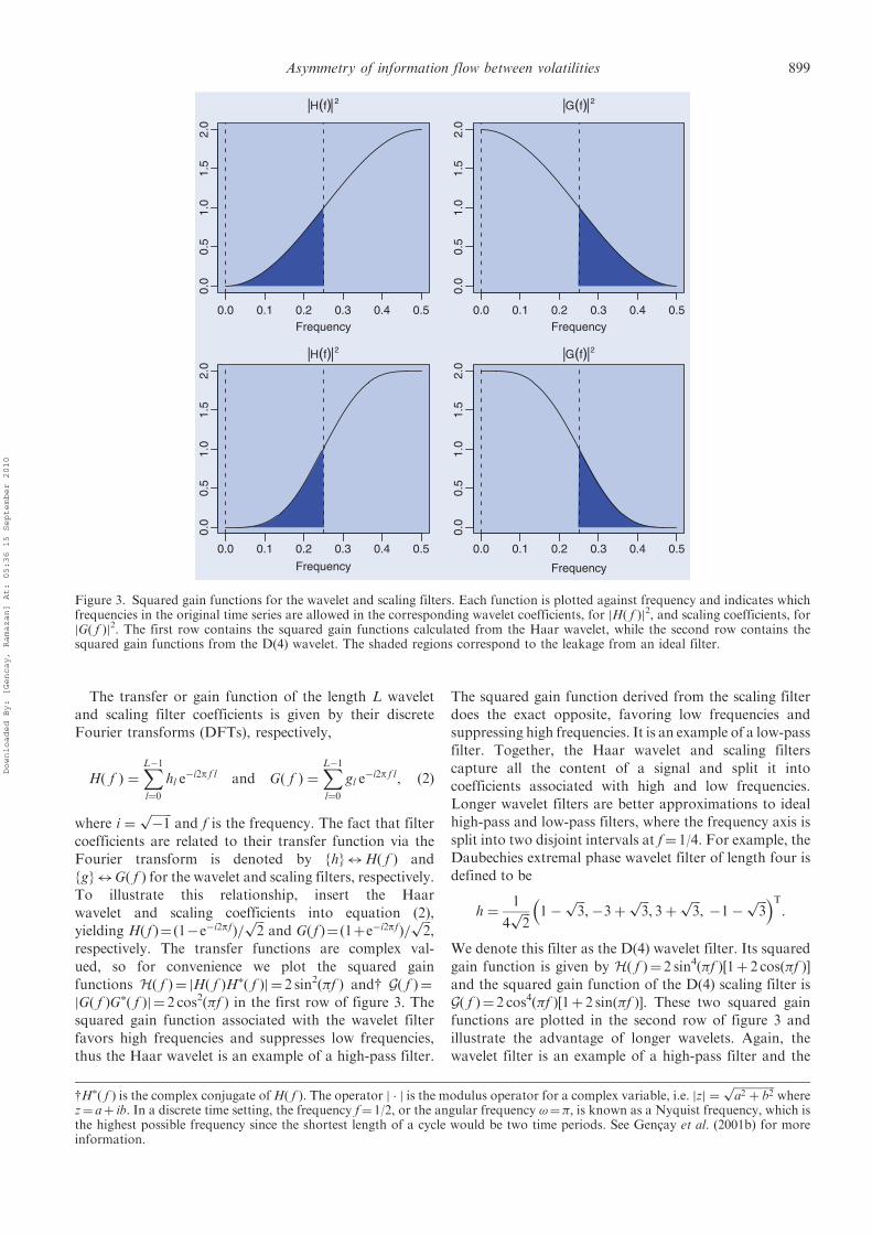
The transfer or gain function of the length L wavelet

and scaling filter coefficients is given by their discrete

Fourier transforms (DFTs), respectively,

Hð f Þ ¼XL�1l¼0

hl e�i2p f l and Gð f Þ ¼

XL�1l¼0

gl e�i2p f l, ð2Þ

where i ¼ffiffiffiffiffiffiffi�1p

and f is the frequency. The fact that filter

coefficients are related to their transfer function via the

Fourier transform is denoted by {h}$H( f ) and

{g}$G( f ) for the wavelet and scaling filters, respectively.

To illustrate this relationship, insert the Haar

wavelet and scaling coefficients into equation (2),

yielding Hð f Þ¼ð1�e�i2pfÞ=ffiffiffi2p

and Gð f Þ¼ð1þe�i2pfÞ=ffiffiffi2p

,

respectively. The transfer functions are complex val-

ued, so for convenience we plot the squared gain

functions H( f )¼ jH( f )H�( f )j ¼ 2 sin2(�f ) andy G( f )¼

jG( f )G�( f )j ¼ 2 cos2(�f ) in the first row of figure 3. The

squared gain function associated with the wavelet filter

favors high frequencies and suppresses low frequencies,

thus the Haar wavelet is an example of a high-pass filter.

The squared gain function derived from the scaling filter

does the exact opposite, favoring low frequencies and

suppressing high frequencies. It is an example of a low-pass

filter. Together, the Haar wavelet and scaling filters

capture all the content of a signal and split it into

coefficients associated with high and low frequencies.

Longer wavelet filters are better approximations to ideal

high-pass and low-pass filters, where the frequency axis is

split into two disjoint intervals at f¼ 1/4. For example, the

Daubechies extremal phase wavelet filter of length four is

defined to be

h ¼1

4ffiffiffi2p 1�

ffiffiffi3p

,�3þffiffiffi3p

, 3þffiffiffi3p

, �1�ffiffiffi3p� �T

:

We denote this filter as the D(4) wavelet filter. Its squared

gain function is given by H( f )¼ 2 sin4(�f )[1þ 2 cos(�f )]and the squared gain function of the D(4) scaling filter is

G( f )¼ 2 cos4(�f )[1þ 2 sin(�f )]. These two squared gain

functions are plotted in the second row of figure 3 and

illustrate the advantage of longer wavelets. Again, the

wavelet filter is an example of a high-pass filter and the

0.0 0.1 0.2 0.3 0.4 0.5

0.0

0.5

1.0

1.5

2.0

H(f) 2

Frequency0.0 0.1 0.2 0.3 0.4 0.5

0.0

0.5

1.0

1.5

2.0

G(f) 2

Frequency

0.0 0.1 0.2 0.3 0.4 0.5

0.0

0.5

1.0

1.5

2.0

H(f) 2

Frequency

0.0 0.1 0.2 0.3 0.4 0.5

0.0

0.5

1.0

1.5

2.0

G(f) 2

Frequency

Figure 3. Squared gain functions for the wavelet and scaling filters. Each function is plotted against frequency and indicates whichfrequencies in the original time series are allowed in the corresponding wavelet coefficients, for jH( f )j2, and scaling coefficients, forjG( f )j2. The first row contains the squared gain functions calculated from the Haar wavelet, while the second row contains thesquared gain functions from the D(4) wavelet. The shaded regions correspond to the leakage from an ideal filter.

yH�( f ) is the complex conjugate ofH( f ). The operator j � j is the modulus operator for a complex variable, i.e. jzj ¼ffiffiffiffiffiffiffiffiffiffiffiffiffiffiffia2 þ b2p

wherez¼ aþ ib. In a discrete time setting, the frequency f¼ 1/2, or the angular frequency !¼�, is known as a Nyquist frequency, which isthe highest possible frequency since the shortest length of a cycle would be two time periods. See Gencay et al. (2001b) for moreinformation.



scaling filter is an example of a low-pass filter but thedifferentiation between frequencies above and belowf¼ 1/4 is much improved over the Haar wavelet andscaling filters. This is seen by the steeper ascent (descent)of the squared gain functions for the wavelet (scaling)filters and the longer plateaus at each end of thefrequency interval. Additional information regardingwavelet filters, including the Haar and longer compactlysupported orthogonal wavelets, and their properties maybe found in, for example, Mallat (1998) and Gencay et al.(2001b).

2.2. The discrete wavelet transform

In this section we introduce notation and concepts inorder to compute the discrete wavelet transform (DWT)of a finite-length vector of observations. There are avariety of ways to express the basic DWT. We proceed byintroducing the DWT as a simple matrix operation. Let Xbe a dyadic length vector (N¼ 2 J) of observations. Thelength N vector of discrete wavelet coefficients W isobtained via W¼WX, whereW is an N�N orthonormalmatrix defining the DWT. The vector of waveletcoefficients may be organized into Jþ 1 vectors

W ¼ ðW1,W2, . . . ,WJ,VJÞT, ð3Þ

where Wj is a length N/2 j vector of wavelet coefficientsassociated with changes on a scale of length �j¼ 2 j�1, VJ

is a length N/2 J vector of scaling coefficients associatedwith averages on a scale of length 2 J

¼ 2�J, and WT is thematrix transpose of the vector W. Wavelet coefficients areobtained by projecting the wavelet filter onto the vector ofobservations. Since Daubechies wavelets may be consid-ered as generalized differences (Gencay et al. 2001b,section 4.3), we prefer to characterize the waveletcoefficients this way. For example, a unit scaleDaubechies wavelet filter is a generalized difference oflength one; that is, the wavelet filter is essentially takingthe difference between two consecutive observations. Wecall this the wavelet scale of length �1¼ 20¼ 1. A scaletwo Daubechies wavelet filter is a generalized differenceof length two; that is, the wavelet filter first averagesconsecutive pairs of observations and then takes thedifference of these averages. We call this the wavelet scaleof length �2¼ 21¼ 2. The scale length increases by powersof two as a function of scale.

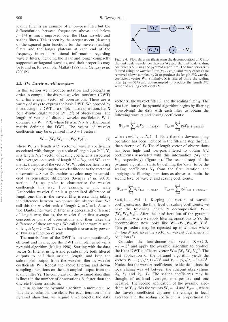
The matrix form of the DWT is not computationallyefficient and in practice the DWT is implemented via apyramid algorithm (Mallat 1998). Starting with the datavector X, filter it using h and g, subsample both filteredoutputs to half their original length, and keep thesubsampled output from the wavelet filter as waveletcoefficients W1. Repeat the above filtering and down-sampling operations on the subsampled output from thescaling filter V1. The complexity of the pyramid algorithmis linear in the number of observations N, faster than thediscrete Fourier transform.

Let us go into the pyramid algorithm in more detail sothat the calculations are clear. For each iteration of thepyramid algorithm, we require three objects: the data

vector X, the wavelet filter h, and the scaling filter g. Thefirst iteration of the pyramid algorithm begins by filtering(convolving) the data with each filter to obtain thefollowing wavelet and scaling coefficients:

W1,t ¼XL�1l¼0

hlX2tþ1�lmodN, V1,t ¼XL�1l¼0

glX2tþ1�lmodN,

where t¼ 0, 1, . . . ,N/2� 1. Note that the downsamplingoperation has been included in the filtering step throughthe subscript of Xt. The N length vector of observationshas been high- and low-pass filtered to obtain N/2coefficients associated with this information (W1 andV1, respectively) (figure 4). The second step of thepyramid algorithm starts by defining the ‘data’ to be thescaling coefficients V1 from the first iteration andapplying the filtering operations as above to obtain thesecond level of wavelet and scaling coefficients:

W2,t ¼XL�1l¼0

hlV1,2tþ1�lmodN, V2,t ¼XL�1l¼0

glV1,2tþ1�lmodN,

t¼ 0, 1, . . . ,N/4� 1. Keeping all vectors of waveletcoefficients, and the final level of scaling coefficients, wehave the following length N decomposition: W¼

(W1,W2,V2)T. After the third iteration of the pyramid

algorithm, where we apply filtering operations to V2, thedecomposition now looks like W¼ (W1,W2,W3,V3)

T.This procedure may be repeated up to J times whereJ¼ log2N and gives the vector of wavelet coefficients inequation (3).

Consider the four-dimensional vector X¼ (2, 3,�2,�1)T and apply the pyramid algorithm to producethe Haar DWT coefficient vector W¼ (W1,W2,V2)

T. Thefirst application of the pyramid algorithm yields thevectors W1 ¼ ð1=

ffiffiffi2p

, 1=ffiffiffi2pÞT and V1 ¼ ð5=

ffiffiffi2p

, �3=ffiffiffi2pÞT.

Notice that the wavelet coefficients are identical, since thelocal change was þ1 between the adjacent observationsX0, X1 and X2, X3. The scaling coefficients may bethought of as local averages, one positive and onenegative. The second application of the pyramid algo-rithm to V1 yields the vectors W2¼�4 and V2¼ 1, wherethe wavelet coefficient captures the change in localaverages and the scaling coefficient is proportional to

Figure 4. Flow diagram illustrating the decomposition of X intothe unit scale wavelet coefficients W1 and the unit scale scalingcoefficients V1 using the pyramid algorithm. The time series X isfiltered using the wavelet filter {h}$H( f ) and every other valueremoved (downsampled by 2) to produce the length N/2 waveletcoefficient vector W1. Similarly, X is filtered using the scalingfilter {g}$G( f ) and downsampled to produce the length N/2vector of scaling coefficients V1.



the sample mean. Thus, the vector of Haar DWTcoefficients for X is

W ¼1ffiffiffi2p ,

1ffiffiffi2p , �4, 1

� �T

: ð4Þ

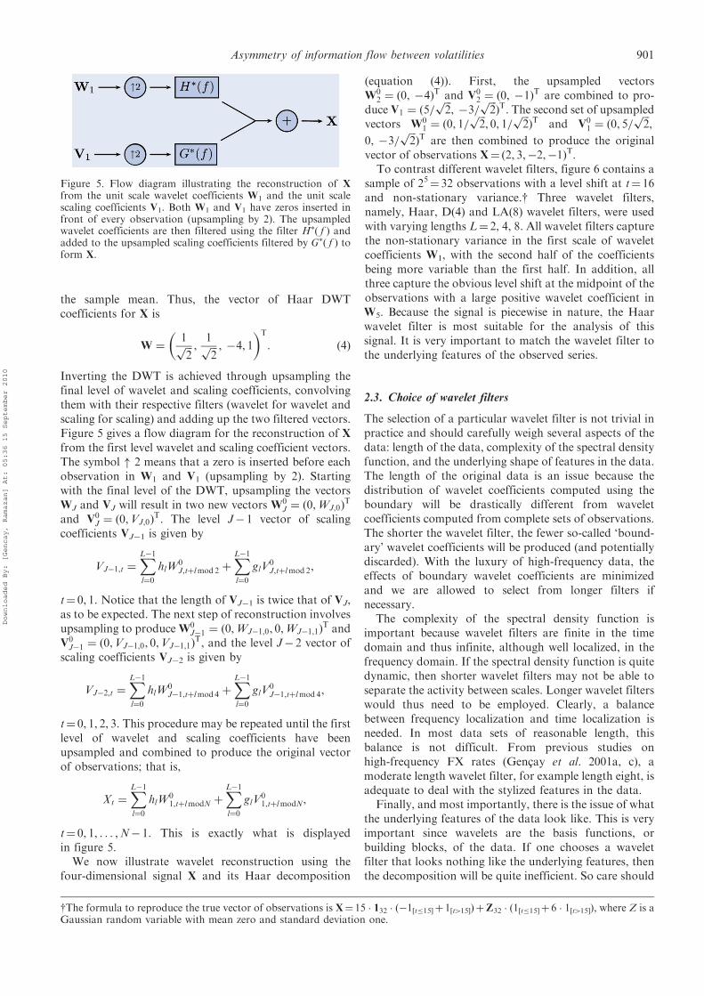
Inverting the DWT is achieved through upsampling thefinal level of wavelet and scaling coefficients, convolvingthem with their respective filters (wavelet for wavelet andscaling for scaling) and adding up the two filtered vectors.Figure 5 gives a flow diagram for the reconstruction of Xfrom the first level wavelet and scaling coefficient vectors.The symbol " 2 means that a zero is inserted before eachobservation in W1 and V1 (upsampling by 2). Startingwith the final level of the DWT, upsampling the vectorsWJ and VJ will result in two new vectors W0

J ¼ ð0,WJ,0ÞT

and V0J ¼ ð0,VJ,0Þ

T. The level J� 1 vector of scalingcoefficients VJ�1 is given by

VJ�1,t ¼XL�1l¼0

hlW0J,tþlmod 2 þ

XL�1l¼0

glV0J,tþlmod 2,

t¼ 0, 1. Notice that the length of VJ�1 is twice that of VJ,as to be expected. The next step of reconstruction involvesupsampling to produceW0

J�1 ¼ ð0,WJ�1,0, 0,WJ�1,1ÞT and

V0J�1 ¼ ð0,VJ�1,0, 0,VJ�1,1Þ

T, and the level J� 2 vector ofscaling coefficients VJ�2 is given by

VJ�2,t ¼XL�1l¼0

hlW0J�1,tþlmod 4 þ

XL�1l¼0

glV0J�1,tþlmod 4,

t¼ 0, 1, 2, 3. This procedure may be repeated until the firstlevel of wavelet and scaling coefficients have beenupsampled and combined to produce the original vectorof observations; that is,

Xt ¼XL�1l¼0

hlW01,tþlmodN þ

XL�1l¼0

glV01,tþlmodN,

t¼ 0, 1, . . . ,N� 1. This is exactly what is displayedin figure 5.

We now illustrate wavelet reconstruction using thefour-dimensional signal X and its Haar decomposition

(equation (4)). First, the upsampled vectorsW0

2 ¼ ð0, �4ÞT and V0

2 ¼ ð0, �1ÞT are combined to pro-

duce V1 ¼ ð5=ffiffiffi2p

, �3=ffiffiffi2pÞT. The second set of upsampled

vectors W01 ¼ ð0, 1=

ffiffiffi2p

, 0, 1=ffiffiffi2pÞT and V0

1 ¼ ð0, 5=ffiffiffi2p

,

0, �3=ffiffiffi2pÞT are then combined to produce the original

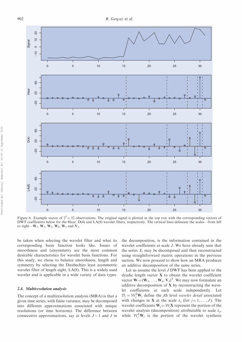
vector of observations X¼ (2, 3,�2,�1)T.To contrast different wavelet filters, figure 6 contains a

sample of 25¼ 32 observations with a level shift at t¼ 16and non-stationary variance.y Three wavelet filters,namely, Haar, D(4) and LA(8) wavelet filters, were usedwith varying lengths L¼ 2, 4, 8. All wavelet filters capturethe non-stationary variance in the first scale of waveletcoefficients W1, with the second half of the coefficientsbeing more variable than the first half. In addition, allthree capture the obvious level shift at the midpoint of theobservations with a large positive wavelet coefficient inW5. Because the signal is piecewise in nature, the Haarwavelet filter is most suitable for the analysis of thissignal. It is very important to match the wavelet filter tothe underlying features of the observed series.

2.3. Choice of wavelet filters

The selection of a particular wavelet filter is not trivial inpractice and should carefully weigh several aspects of thedata: length of the data, complexity of the spectral densityfunction, and the underlying shape of features in the data.The length of the original data is an issue because thedistribution of wavelet coefficients computed using theboundary will be drastically different from waveletcoefficients computed from complete sets of observations.The shorter the wavelet filter, the fewer so-called ‘bound-ary’ wavelet coefficients will be produced (and potentiallydiscarded). With the luxury of high-frequency data, theeffects of boundary wavelet coefficients are minimizedand we are allowed to select from longer filters ifnecessary.

The complexity of the spectral density function isimportant because wavelet filters are finite in the timedomain and thus infinite, although well localized, in thefrequency domain. If the spectral density function is quitedynamic, then shorter wavelet filters may not be able toseparate the activity between scales. Longer wavelet filterswould thus need to be employed. Clearly, a balancebetween frequency localization and time localization isneeded. In most data sets of reasonable length, thisbalance is not difficult. From previous studies onhigh-frequency FX rates (Gencay et al. 2001a, c), amoderate length wavelet filter, for example length eight, isadequate to deal with the stylized features in the data.

Finally, and most importantly, there is the issue of whatthe underlying features of the data look like. This is veryimportant since wavelets are the basis functions, orbuilding blocks, of the data. If one chooses a waveletfilter that looks nothing like the underlying features, thenthe decomposition will be quite inefficient. So care should

yThe formula to reproduce the true vector of observations is X¼ 15 � 132 � (�1[t�15]þ 1[t415])þZ32 � (1[t�15]þ 6 � 1[t415]), where Z is aGaussian random variable with mean zero and standard deviation one.

Figure 5. Flow diagram illustrating the reconstruction of X

from the unit scale wavelet coefficients W1 and the unit scalescaling coefficients V1. Both W1 and V1 have zeros inserted infront of every observation (upsampling by 2). The upsampledwavelet coefficients are then filtered using the filter H�( f ) andadded to the upsampled scaling coefficients filtered by G�( f ) toform X.



be taken when selecting the wavelet filter and what itscorresponding basis function looks like. Issues ofsmoothness and (a)symmetry are the most commondesirable characteristics for wavelet basis functions. Forthis study, we chose to balance smoothness, length andsymmetry by selecting the Daubechies least asymmetricwavelet filter of length eight, LA(8). This is a widely usedwavelet and is applicable in a wide variety of data types.

2.4. Multiresolution analysis

The concept of a multiresolution analysis (MRA) is that agiven time series, with finite variance, may be decomposedinto different approximations associated with uniqueresolutions (or time horizons). The difference betweenconsecutive approximations, say at levels J� 1 and J in

the decomposition, is the information contained in the

wavelet coefficients at scale J. We have already seen that

the series Xt may be decomposed and then reconstructed

using straightforward matrix operations in the previous

section. We now proceed to show how an MRA produces

an additive decomposition of the same series.Let us assume the level J DWT has been applied to the

dyadic length vector X to obtain the wavelet coefficient

vector W¼ (W1, . . . ,WJ, VJ)T. We may now formulate an

additive decomposition of X by reconstructing the wave-

let coefficients at each scale independently. Let

Dj ¼ WTj Wj define the jth level wavelet detail associated

with changes in X at the scale �j (for j¼ 1, . . . , J ). The

wavelet coefficientsWj¼W jX represent the portion of the

wavelet analysis (decomposition) attributable to scale �j,

while WTj Wj is the portion of the wavelet synthesis

0 5 10 15 20 25 30

−10

010

20

Sig

nal

0 5 10 15 20 25 30

−20

2060

Haa

r

0 5 10 15 20 25 30

−20

2060

D(4

)

0 5 10 15 20 25 30

−20

2060

LA(8

)

Figure 6. Example vector of 25¼ 32 observations. The original signal is plotted in the top row with the corresponding vectors ofDWT coefficients below for the Haar, D(4) and LA(8) wavelet filters, respectively. The vertical lines delineate the scales—from leftto right—W1, W2, W3, W4, W5 and V5.



(reconstruction) attributable to scale �j. For a length

N¼ 2 J vector of observations, the vector SJ ¼ VTJVJ is

equal to the sample mean of the observations.A multiresolution analysis (MRA) may now be

defined via

Xt ¼XJj¼1

Dj, t þ SJ, t ¼ 0, . . . ,N� 1: ð5Þ

That is, each observation Xt is a linear combination of

wavelet detail coefficients at time t. Let Sj ¼PJþ1

k¼j Dk

define the jth level wavelet smooth (for 1� j� J ). Whereasthe wavelet detail Dj is associated with variations at aparticular scale, Sj is a cumulative sum of these variationsand will be smoother and smoother as j increases. In fact,

X� Sj ¼Pj

k¼1Dk so that only lower-scale details(high-frequency features) from the original seriesremain. The jth level wavelet rough characterizes theremaining lower-scale details through

Rj ¼Xjk¼1

Dk, 1 � j � J:

The wavelet rough Rj is what remains after removingthe wavelet smooth from the vector of observations.

For smaller j the wavelet rough is less smooth. A vector ofobservations may thus be decomposed through a waveletsmooth and rough via Xt¼Sj,tþRj,t, for all j, t, which isequivalent to equation (5). The wavelet details are thedifferences between either adjacent wavelet smooths oradjacent wavelet roughs.

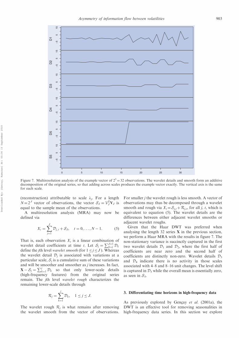
Given that the Haar DWT was preferred whenanalysing the length 32 series X in the previous section,we perform a Haar MRA with the results in figure 7. Thenon-stationary variance is succinctly captured in the firsttwo wavelet details D1 and D2, where the first half ofcoefficients are near zero and the second half ofcoefficients are distinctly non-zero. Wavelet details D3

and D4 indicate there is no activity in those scalesassociated with 4–8 and 8–16 unit changes. The level shiftis captured in D5 while the overall mean is essentially zero,as seen in S5.

3. Differentiating time horizons in high-frequency data

As previously explored by Gencay et al. (2001a), theDWT is an effective tool for removing seasonalities inhigh-frequency data series. In this section we explore

−5

515

D1

−5

515

D2

−5

515

D3

−5

515

D4

−5

515

D5

−5

515

S5

0 5 10 15 20 25 30

Figure 7. Multiresolution analysis of the example vector of 25¼ 32 observations. The wavelet details and smooth form an additivedecomposition of the original series, so that adding across scales produces the example vector exactly. The vertical axis is the samefor each scale.



the ability of a multi-scale decomposition (specificallythe MRA described in section 2.4) to reproduce thecorrelation structure of realized volatility found atdifferent sampling rates of high-frequency data. Themulti-scale decomposition of realized volatility is ademonstration that modeling high-frequency realizedvolatility in the wavelet domain captures the features ata variety of sampling rates simultaneously, whereascurrent methodology only models one fixed samplingfrequency.

3.1. Actual realized volatility

We follow Andersen et al. (2001) and Dacorogna et al.(2001) to define realized volatility (or actual realizedvolatility) via

�2t,� ¼X��1k¼0

r2tþk=�, ð6Þ

where rtþk/�¼ ptþk/�� ptþ(k�1)/� are continuously com-pounded returns sampled � times per day. The raw 5-minreturn series was obtained from Olsen & Associatesspanning January 1, 1987, through December 31, 1998,and excludes weekends (defined to be Friday 21:05 GMTuntil Sunday 21:00 GMT). This results in a series of901,152 high-frequency return observations, or 3129 daysof data. Hence, the sampling rate � will vary depending onthe level of aggregation needed to calculate realizedvolatility at coarser levels of time. For example, �¼ 288for daily realized volatility but we will also consider20-min and hourly realized volatility with �¼ 4 and�¼ 12, respectively.

Looking at the definition of realized volatility moreclosely, there are two operations in equation (6). First, afilter of length � is applied to the squared returns witheach value of the filter being one. For dyadic lengths, thisfilter mimics the Haar scaling filter. Then a downsamplingoperation is performed that picks every �th value from thesmoothed return series. Hence, aggregation is related tothe Haar DWT through its use of filtering and down-sampling but it utilizes a non-orthogonal filter.

3.2. Wavelet realized volatility

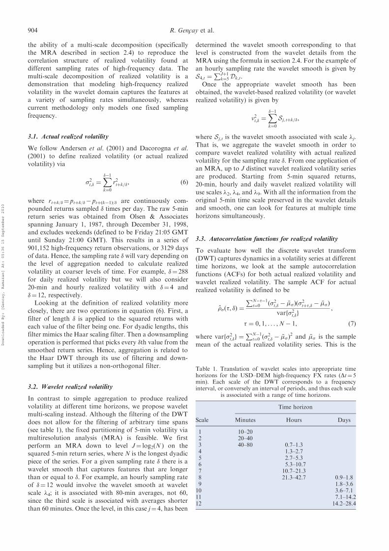
In contrast to simple aggregation to produce realizedvolatility at different time horizons, we propose waveletmulti-scaling instead. Although the filtering of the DWTdoes not allow for the filtering of arbitrary time spans(see table 1), the fixed partitioning of 5-min volatility viamultiresolution analysis (MRA) is feasible. We firstperform an MRA down to level J¼ log2(N ) on thesquared 5-min return series, where N is the longest dyadicpiece of the series. For a given sampling rate � there is awavelet smooth that captures features that are longerthan or equal to �. For example, an hourly sampling rateof �¼ 12 would involve the wavelet smooth at waveletscale �4; it is associated with 80-min averages, not 60,since the third scale is associated with averages shorterthan 60 minutes. Once the level, in this case j¼ 4, has been

determined the wavelet smooth corresponding to thatlevel is constructed from the wavelet details from theMRA using the formula in section 2.4. For the example ofan hourly sampling rate the wavelet smooth is given byS4,t ¼

PJþ1k¼5Dk,t.

Once the appropriate wavelet smooth has beenobtained, the wavelet-based realized volatility (or waveletrealized volatility) is given by

�2t,� ¼X��1k¼0

Sj, tþk=�,

where Sj,t is the wavelet smooth associated with scale �j.That is, we aggregate the wavelet smooth in order tocompare wavelet realized volatility with actual realizedvolatility for the sampling rate �. From one application ofan MRA, up to J distinct wavelet realized volatility seriesare produced. Starting from 5-min squared returns,20-min, hourly and daily wavelet realized volatility willuse scales �2, �4, and �9. With all the information from theoriginal 5-min time scale preserved in the wavelet detailsand smooth, one can look for features at multiple timehorizons simultaneously.

3.3. Autocorrelation functions for realized volatility

To evaluate how well the discrete wavelet transform(DWT) captures dynamics in a volatility series at differenttime horizons, we look at the sample autocorrelationfunctions (ACFs) for both actual realized volatility andwavelet realized volatility. The sample ACF for actualrealized volatility is defined to be

��ð�, �Þ ¼

PN��1t¼0 ð�2t,� � ��Þð�

2tþ�,� � ��Þ

varf�2t,�g,

� ¼ 0, 1, . . . ,N� 1, ð7Þ

where varf�2t,�g ¼PN�1

t¼0 ð�2t,� � ��Þ

2 and �� is the samplemean of the actual realized volatility series. This is the

Table 1. Translation of wavelet scales into appropriate timehorizons for the USD–DEM high-frequency FX rates (Dt¼ 5min). Each scale of the DWT corresponds to a frequencyinterval, or conversely an interval of periods, and thus each scale

is associated with a range of time horizons.

Time horizon

Scale Minutes Hours Days

1 10–202 20–403 40–80 0.7–1.34 1.3–2.75 2.7–5.36 5.3–10.77 10.7–21.38 21.3–42.7 0.9–1.89 1.8–3.610 3.6–7.111 7.1–14.212 14.2–28.4



usual definition of the covariance for the actual realized

volatility series at lag � divided by the variance

(covariance at lag 0) of the actual realized volatility

series. The sample ACF ��ð�, �Þ estimates the true ACF of

actual realized volatility at a given sampling rate.The sample ACF for wavelet realized volatility is

defined similarly via

��ð�, �Þ ¼

PN��1t¼0 ð�2t,� � ��Þð�

2tþ�,� � ��Þ

varf�2t,�g þ varf�2t,�ðRj Þg,

� ¼ 0, 1, . . . ,N� 1, ð8Þ

where varf�2t,�g ¼PN�1

t¼0 ð�2t,� � ��Þ

2 and �� is the sample

mean of the wavelet realized volatility series. The second

term in the denominator of equation (8) is the remainder

of the variance in the MRA coefficients not accounted for

by the wavelet smooth Sj. Recall, the wavelet rough is

computed via Rj ¼Pj

k¼1Dk and is then aggregated to

form �2t,�ðRj Þ ¼P��1

k¼0Rj, tþk=�. Finally, the variance of the

wavelet realized volatility based on the wavelet rough is

given by varf�2t,�ðRj Þg ¼PN�1

t¼0 ½�2t,�ðRj Þ � ��ðRj Þ�

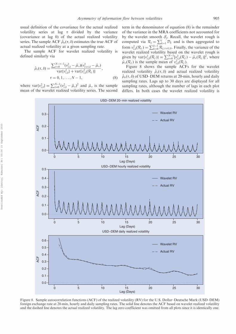
2, where��ðRj Þ is the sample mean of �2t,�ðRj Þ.Figure 8 shows the sample ACFs for the wavelet

realized volatility ��ð�, �Þ and actual realized volatility

��ð�, �Þ of USD–DEM returns at 20-min, hourly and daily

sampling rates. Lags up to 30 days are displayed for all

sampling rates, although the number of lags in each plot

differs. In both cases the wavelet realized volatility is

302520151050

302520151050

302520151050

0.0

0.1

0.2

0.3

Lag (Days)

AC

F

USD−DEM 20−min realized volatility

Wavelet RV

Actual RV

0.0

0.1

0.2

0.3

0.4

0.5

Lag (Days)

AC

F

USD−DEM hourly realized volatility

Wavelet RV

Actual RV

0.0

0.1

0.2

0.3

0.4

0.5

0.6

Lag (Days)

AC

F

USD−DEM daily realized volatility

Wavelet RV

Actual RV

Figure 8. Sample autocorrelation functions (ACF) of the realized volatility (RV) for the U.S. Dollar–Deutsche Mark (USD–DEM)foreign exchange rate at 20-min, hourly and daily sampling rates. The solid line denotes the ACF based on wavelet realized volatilityand the dashed line denotes the actual realized volatility. The lag zero coefficient was omitted from all plots since it is identically one.



virtually indistinguishable from the actual realized vola-tility at all lags except the first. For daily realizedvolatility, the wavelet-based version exhibits less variationfrom lag to lag due to the fact that the high-frequencycontent was removed via the MRA.

4. Wavelet-based hidden Markov Trees

4.1. Introduction

Modeling in the wavelet domain usually ignores thecorrelation between wavelet coefficients, falling back onthe assumption that the DWT is a whitening transform.Indeed, for a wide range of naturally occurring time seriesthe wavelet coefficients may be treated as uncorrelatedand Gaussian. These assumptions are not valid in thecontext of analysing high-frequency FX rates. First, sincethe quantity of interest is volatility there is no opportunityto assume a Gaussian distribution for the observed series.Second, the unknown and potentially complex correlationstructure in the series most likely does not produceapproximately uncorrelated wavelet coefficients. We pro-pose to borrow a probabilistic model from signalprocessing and apply it to the wavelet decomposition ofa high-frequency volatility series. By taking advantageof the tree-based structure of the DWT, we provide anefficient representation and estimation technique of theunderlying joint distribution of the wavelet coefficients.Through this representation the multi-scale decomposi-tion of the volatility series is classified into a state of highor low volatility.

In the context of signal processing applications, Crouseet al. (1998) proposed a variety of hidden Markov modelsfor wavelet decompositions of one- and two-dimensionaldata sets (time series and images). The assumption ofuncorrelated wavelet coefficients was replaced by thepossibility of allowing correlation between scales of the

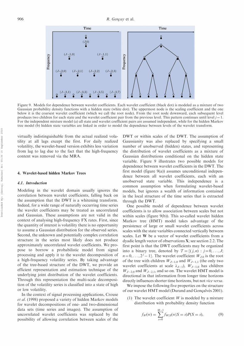
DWT or within scales of the DWT. The assumption ofGaussianity was also replaced by specifying a smallnumber of unobserved (hidden) states, and representingthe distribution of wavelet coefficients as a mixture ofGaussian distributions conditional on the hidden statevariable. Figure 9 illustrates two possible models fordependence between wavelet coefficients in the DWT. Thefirst model (figure 9(a)) assumes unconditional indepen-dence between all wavelet coefficients, each with anunobserved state variable. This independence is acommon assumption when formulating wavelet-basedmodels, but ignores a wealth of information containedin the local structure of the time series that is extractedthrough the DWT.

One possible model of dependence between waveletcoefficients is to allow association between scales but notwithin scales (figure 9(b)). This so-called wavelet hiddenMarkov tree (HMT) model takes advantage of thepersistence of large or small wavelet coefficients acrossscales with the state variables connected vertically betweenscales. Let W be a vector of wavelet coefficients from adyadic length vector of observationsX; see section 2.2. Thefirst point is that the DWT coefficients may be organizedinto a binary tree, denoted by T ¼ {( j, n) : j¼ 0, . . . , J;n¼ 0, . . . , 2 j

� 1}. The wavelet coefficient WJ,0 is the rootof the tree with children WJ�1,0 and WJ�1,1 (the only twowavelet coefficients at scale �J�1), WJ�1,0 has childrenWJ�2,0 andWJ�2,1, and so on. The wavelet HMT model isdirectional in that information from longer time horizonsdirectly influences shorter time horizons, but not vice versa.

We impose the following five properties on the structureof our wavelet HMTmodel (Durand andGoncalves 2001).

(1) The wavelet coefficient W is modeled by a mixturedistribution with probability density function

fWðwÞ ¼XM�1s¼0

fWjSðwjS ¼ sÞPðS ¼ sÞ, ð9Þ

Figure 9. Models for dependence between wavelet coefficients. Each wavelet coefficient (black dot) is modeled as a mixture of twoGaussian probability density functions with a hidden state (white dot). The uppermost node is the scaling coefficient and the onebelow it is the coarsest wavelet coefficient (which we call the root node). From the root node downward, each subsequent levelproduces two children for each state and the wavelet coefficient pair from the previous level. This pattern continues until level j¼ 1.For the independent mixture model (a) all state and wavelet coefficient pairs are assumed independent, while for the hidden Markovtree model (b) hidden state variables are linked in order to model the dependence between levels of the wavelet transform.



where S is a discrete random variable (the hidden

state) with M possible values.(2) Let S¼ (S1, . . . ,SJ,SVJ

)T define the state vector

associated with the vector of wavelet coefficients

W, indexed in the same way. Thus, the state vector

may be organized as a binary tree rooted at SJ,0

and read from right to left. Since we are using two

indices, one for the scale and one for the location

within scale, the parent of Sj,n is given explicitly by

Sjþ1,bn/2c for j¼ 2, . . . , J.y The children of Sj,n are

given explicitly by Sj�1,2n and Sj�1,2nþ1. The

notation for state variables in the binary tree is

illustrated in figure 9(a) using only the subscripts.

The root is SJ,0, the next level down from left to

right is SJ�1,0 and SJ�1,1; the next level down is

SJ�2,0, SJ�2,1, SJ�2,2 and SJ�2,3; and so on.

Dependence between scales in the state variables

is illustrated in figure 9(b) and uses an identical

labeling scheme.(3) The state variable Sj,n is independent of all other

states given its parent and children, i.e.

PðSj, njfSa,bga 6¼j, b6¼nÞ ¼ PðSj, njSjþ1,bn=2c,Sj�1,2n,Sj�1,2nþ1Þ:

(4) The joint probability distribution of the wavelet

coefficient vector W is independent given the state

vector S, i.e.

fWjSðWÞ ¼Yð j, nÞ2T

fWj,njSðwj, nÞ:

(5) The wavelet coefficient Wj,n is independent of all

other states given its own state, i.e.

fWj,njSðwj, nÞ ¼ fWj,njSj, nðwj, nÞ, for all ð j, nÞ 2 T :

The last two properties are known as conditional

independence properties. We assume the mixture distri-

bution for W is based on Gaussian probability density

functions (PDFs) with mean s and variance �2s ,

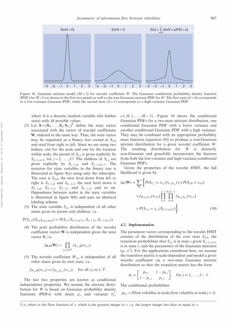
s2 {0, 1, . . . ,M� 1}. Figure 10 shows the conditionalGaussian PDFs for a two-state mixture distribution, oneconditional Gaussian PDF with a lower variance andanother conditional Gaussian PDF with a high variance.They may be combined with an appropriate probabilitymass function (equation (9)) to produce a non-Gaussianmixture distribution for a given wavelet coefficient W.The resulting distribution for W is distinctlynon-Gaussian and gracefully incorporates the featuresfrom both the low-variance and high-variance conditionalGaussian PDFs.

Given the properties of the wavelet HMT, the fulllikelihood is given by

fWðWÞ ¼XS

�PðSVJ

¼ sVJÞ fVJjSVJ

ðvJÞPðSJ,0 ¼ sJ,0Þ

�fWJ,0jSJ,0ðwJ,0Þ

YJ�1j¼1

YN=2j�1n¼0

fWj,njSj, nðwj, nÞ

�PðSj, n ¼ sj, njSjþ1,bn=2cÞ

�: ð10Þ

4.2. Implementation

The parameter vector corresponding to the wavelet HMTconsists of the distribution of the root state SJ,0, thetransition probabilities that Sj,n is in state s given Sj�1,bn/2c

is in state r, and the parameters of the Gaussian mixtures(, �2). For the applications considered here, we assumethe transition matrix is scale-dependent and model a givenwavelet coefficient via a two-state Gaussian mixturedistribution so that the transition matrix has the form

Aj ¼p0, j 1� p0, j

1� p1, j p1, j

, for j ¼ 1, . . . , J� 1.

The conditional probabilities

p0, j¼Pðlow volatility at scale jjlow volatility at scale jþ1Þ

f(w|S = 0) f(w|S = 1) f(w) =s=0

1f(w|S = s)P(S = s)

−3 −2 −1 0 1 2 3 −3 −2 −1 0 1 2 3 −3 −2 −1 0 1 2 3

S

Figure 10. Gaussian mixture model (M¼ 2) for wavelet coefficient W. The Gaussian conditional probability density function(PDF) forW jS are shown in the first two panels as well as the non-Gaussian mixture PDF forW. The first state (S¼ 0) correspondsto a low-variance Gaussian PDF, while the second state (S¼ 1) corresponds to a high-variance Gaussian PDF.

ybxc refers to the floor function of x, which is the greatest integer in x, i.e. the largest integer less than or equal to x.



and

p1, j ¼ Pðhigh volatility at scale j

jhigh volatility at scale jþ 1Þ

reflect the persistence of large and small waveletcoefficients from long time horizons to shorter timehorizons, respectively. We expect the transition probabil-ity from low to high volatility (1� p0, j) to be quite small,and therefore p0, j� 1 for most scales. The main parameterof interest is pi, j. Given a high volatility state at scale jþ 1,how likely is a high volatility state to persist to scale j?The complete parameter vector for the wavelet HMTmodel is explicitly given by

¼ ð p0,1, p1,1, . . . , p0, J, p1, J,0,1,

�20,1, . . . ,0, J, �20, J1,1, �

21,1, . . . ,1, J, �

21, JÞ,

and includes all transition probabilities and parametersassociated with the Gaussian PDFs. The DWT ensuresthat the expected value of all wavelet coefficients will bezero when using a wavelet filter of sufficient length. Wethus make the assumption that s, j¼ 0 for all s and j.

Maximum likelihood estimation of the parametervector cannot be performed directly on equation (10).An adaptation of the Expected Maximization (EM)algorithm is applied to this problem where the modelparameters and distribution of the hidden states S areestimated jointly, given the observed wavelet coefficientsW. For the estimation step, an upward-downward algo-rithm for calculating the log-likelihood of the waveletHMT was developed by Crouse et al. (1998). Theupward-downward algorithm is similar to the well-knownforward-backward algorithm for hidden Markov chains(Baum 1972).y

The wavelet HMT model is such that dependencebetween wavelet coefficients is allowed only betweenscales. That is, if one pictures a binary tree associatingwavelet coefficients (figure 9(b)), there are no linksbetween adjacent wavelet coefficients within scales—only between and then only from coarse to fine resolutionin time. The intuition behind this dependence structure isthat if there exists a large wavelet coefficient at a giventime horizon (implying a local oscillation with a largeamplitude), then at least one of the wavelet coefficientscomputed using the same data at a shorter time horizonwill also be large. That being said, the transitionprobabilities and parameters of the corresponding mix-ture distribution are estimated using all wavelet coeffi-cients across time. In this respect, the model uses allavailable information for parameter estimation, since allwavelet coefficients are used.

However, one should keep in mind that each waveletcoefficient carries only local information. Once theparameter estimates have been obtained for the waveletHMT model, the wavelet coefficients may be classified

into one of the M states in the mixture distribution usingthe Vitterbi algorithm; see, for example, Rabiner (1989)and references therein. Let �j,n be the sequence of statesand wavelet coefficients for Wj,n on the hidden Markovtree. The Vitterbi algorithm recursively calculates thesequence of states with highest probability from top tobottom using the transition probabilities from the waveletHMT model. Because of the conditional dependencestructure of the model, the Vitterbi algorithm onlyoperates on the states from a small set of waveletcoefficients—the parent and children relative to Wj,n.Note, wavelet coefficients are associated with either highor low volatility since the mean is identically zero for bothGaussian PDFs.

The exact location of volatility bursts in the waveletdomain relies on how the phase information was treatedin the original decomposition. Wavelet coefficientsobtained from most implementations of the DWT willexhibit some translation in time. This is accounted forbefore classification.z

5. Wavelet HMT models for high-frequency data

5.1. USD-DEM volatility

Our variable of interest is the realized volatility at thehigh-frequency 5-min sampling rate. The 5-min foreignexchange (FX) return is defined as

rt,5 ¼ logPt � logPt�1,

where Pt is the FX price at time t. The FX volatility isdefined by squaring 5-min return r2t,5. We estimated atwo-state wavelet HMT model on a span ofN¼ 219¼ 524,288 observations, from January 4, 1987 toDecember 27, 1993. This is the largest dyadic-lengthvector that is less than or equal to the available samplesize of just under 1 million FX rates. For reference, table 1translates wavelet scales ( j¼ 1, . . . , 12) into time horizonsthat span anywhere from several minutes to a month. Weperformed a second analysis on the last N¼ 524,288 (fromJanuary 9, 1992 to December 31, 1998) observations tocheck if the wavelet HMT model produces stableestimates for different, but not disjoint, time spans.

Table 2 provides the conditional probabilities for thescale-dependent transition matrix Aj, j¼ 1, . . . , 12. Thefirst thing we notice is the strong vertical dependencyin low-volatility states. The probability of observing alow-volatility state at time scale j, given that there isa low-volatility state at time scale jþ 1, is almost one at alltime scales, p0,j� 1 for j¼ 1, . . . , 12. For example, giventhat a low-volatility state is observed at a 4–7 day time scale(wavelet scale 10), the probability of observing alow-volatility state at 2–4 days (wavelet scale 9) is 0.96.Similarly, if a low-volatility state is experienced at a

yAn alternative implementation of the upward-downward algorithm from Crouse et al. (1998) may be found in Durand andGoncalves (2001).zThere are approximate phase shifts available for all Daubechies wavelet families in Percival and Walden (2000). Once the DWT hasbeen applied, one must circularly shift each vector of wavelet coefficients by an integer amount.



3–5 hour time scale (wavelet scale 5), the probability of

observing a low-volatility state at 1–3 hours (wavelet scale

4) is 0.99.y Technically, this means that given a wavelet

coefficient associated with low volatility, there is very little

chance that it will produce a wavelet coefficient associated

with high volatility at the lower scale. Hence, the condi-

tional probabilities for low-volatility state to low-volatility

state are almost one. Naturally, the probability of

changing states (from low volatility at time scale j to high

volatility at time scale j� 1) is almost zero, as presented in

table 2. We conclude that vertical dependency in

low-volatility states is an extremely strong one.The vertical dependency among high-volatility states is

not as strong as it is in low-volatility states, especially at

lower time scales. This means that a high-volatility state

(regime) at a given time scale will not guarantee that

wavelet coefficients at the lower time scale will be

associated with high volatility. For example, given a

high-volatility regime at a 4–7 day time scale (wavelet

scale 10), the probability of being a high-volatility regime

at 2–4 days (wavelet scale 9) is 0.78. Similarly, if a

high-volatility regime prevails at a 3–5 hour time scale

(wavelet scale 5), the probability of being in a

high-volatility regime at 1–3 hours (wavelet scale 4) is

0.55. The reason behind this property is that markets calm

down at low time scales (higher frequencies) long before

they do at high time scales (lower frequencies). The

vertical dependency amongst the high-volatility states

implies that the probability of changing states from high

volatility at time scale j to low volatility at time scale j� 1

is relatively high. In particular, the probability of

changing from a high-volatility regime to a low-volatility

regime is approximately 0.50 for time scales of approx-

imately 12 hours or less.These findings establish an important new stylized

property of foreign exchange volatility. In addition to the

well-known horizontal dependence (conditional hetero-scedasticity or volatility clustering and long memory),foreign exchange volatility exhibits strong vertical depen-dence (persistence across different time scales).Furthermore, the vertical dependence of foreign exchangevolatility is asymmetric in the sense that low-to-low-volatility states exhibit a strong dependence while high-to-high-volatility states possess much less dependence.

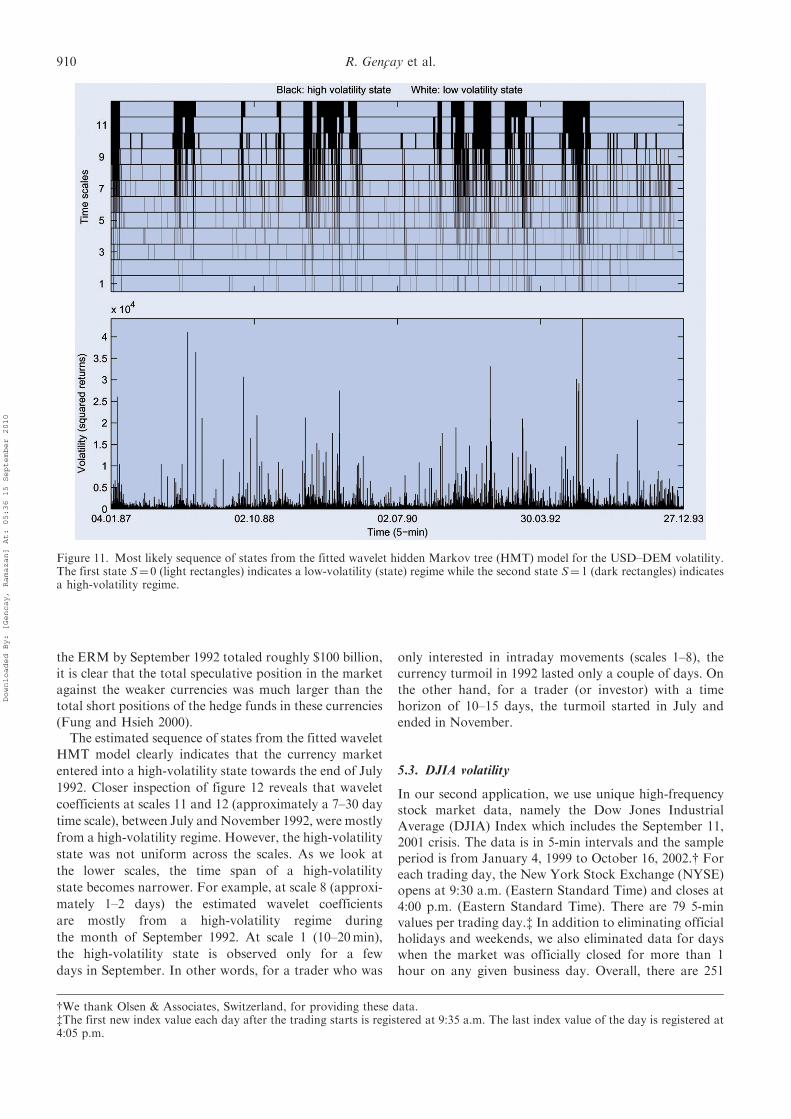
Figure 11 displays the estimates of a sequence of states,with low volatility (light rectangles) or high volatility(dark rectangles), from the wavelet HMT model esti-mated using the first N¼ 219¼ 524,288 5-min volatilities.zA visual inspection of the figure shows the verticaldependency in the foreign exchange volatility. Startingfrom wavelet scale 12 (14–28 day time scale), if thecurrent state is one of low volatility (light rectangle) thenwe again observe a low-volatility state at shorter timescales. However, given a high-volatility state (darkrectangle), we observe high-volatility states less frequentlyat shorter time scales. Notice that dark rectangles becomenarrower as one moves from a long time scale (lowfrequency) to shorter time scales (high frequencies) for agiven period of time. The following section gives anintuitive interpretation of different time scale volatilitystates by zooming in on the second half of 1992 infigure 11.

5.2. Currency turmoil in 1992 at different time scales

International foreign exchange markets experienced oneof their largest turmoils in 1992. The events leading tocurrency turmoil in European economies and interna-tional foreign exchange markets can be tracked back tothe German unification. German authorities decided tofinance the cost of unification through borrowing,causing an increase in German interest rates. Othercurrencies of the European economies were forced toincrease their interest rates to protect the value of theircurrencies against the Deutsche Mark (DM). Speculatorswere already attacking the weaker currencies by bettingthat they could not sustain the parity with the DM. Theincrease in interest rates caused further speculation. ThePortuguese Escudo (PE), Spanish Peseta (SP), Italian Lira(IL), and British Pound (BP) all fell in value against theDM. On September 15, 1992, the BP and IL left theEuropean exchange rate mechanism (ERM) and the PEand the SP were forced to devalue but stayed in the ERM.

George Soros, manager of the Quantum Fund, wasreported to have held a $10 billion USD short position onthe BP and to have made $1 billion for his fund as a resultof the BP’s September devaluation. Some other hedgefunds were also speculating against the BP. Overall, hedgefunds are estimated to have held short positions on theBP, totaling $11.7 billion in excess of 25% of thegovernment’s official reserves in 1992 ($40 billion).Considering the fact that central bank interventions in

Table 2. Conditional probabilities p0, j and p1, j from the scale-dependent transition matrices Aj in the wavelet hidden Markovtree (HMT) model for USD–DEM volatility. The quantityunder the heading Low-to-low, for example, is the probability oflow volatility at scale j given there was low volatility at scalejþ 1. Similarly, the quantity under the heading Low-to-high isthe probability of high volatility at scale j given there was low

volatility at scale jþ 1.

Scale Low-to-low Low-to-high High-to-high High-to-low

11 0.995 0.005 0.981 0.01910 0.865 0.135 0.996 0.0349 0.972 0.028 0.703 0.2978 0.960 0.040 0.782 0.2187 0.950 0.050 0.736 0.2646 0.986 0.014 0.478 0.5225 0.977 0.023 0.554 0.4464 0.985 0.015 0.452 0.5483 0.990 0.010 0.547 0.4532 0.995 0.005 0.505 0.4951 0.988 0.012 0.490 0.510

yTranslations of wavelet scales into appropriate time scales are approximate here. For an exact translation, see table 1.zA second analysis was performed on the last N¼ 219¼ 524,288 (from January 9, 1992 to December 31, 1998) observations from the5-min volatility series of USD–DEM FX rates. The main findings are similar to the first data set.



the ERM by September 1992 totaled roughly $100 billion,

it is clear that the total speculative position in the market

against the weaker currencies was much larger than the

total short positions of the hedge funds in these currencies

(Fung and Hsieh 2000).The estimated sequence of states from the fitted wavelet

HMT model clearly indicates that the currency market

entered into a high-volatility state towards the end of July

1992. Closer inspection of figure 12 reveals that wavelet

coefficients at scales 11 and 12 (approximately a 7–30 day

time scale), between July and November 1992, were mostly

from a high-volatility regime. However, the high-volatility

state was not uniform across the scales. As we look at

the lower scales, the time span of a high-volatility

state becomes narrower. For example, at scale 8 (approxi-

mately 1–2 days) the estimated wavelet coefficients

are mostly from a high-volatility regime during

the month of September 1992. At scale 1 (10–20min),

the high-volatility state is observed only for a few

days in September. In other words, for a trader who was

only interested in intraday movements (scales 1–8), the

currency turmoil in 1992 lasted only a couple of days. On

the other hand, for a trader (or investor) with a time

horizon of 10–15 days, the turmoil started in July and

ended in November.

5.3. DJIA volatility

In our second application, we use unique high-frequencystock market data, namely the Dow Jones IndustrialAverage (DJIA) Index which includes the September 11,2001 crisis. The data is in 5-min intervals and the sampleperiod is from January 4, 1999 to October 16, 2002.y Foreach trading day, the New York Stock Exchange (NYSE)opens at 9:30 a.m. (Eastern Standard Time) and closes at4:00 p.m. (Eastern Standard Time). There are 79 5-minvalues per trading day.z In addition to eliminating officialholidays and weekends, we also eliminated data for dayswhen the market was officially closed for more than 1hour on any given business day. Overall, there are 251

Figure 11. Most likely sequence of states from the fitted wavelet hidden Markov tree (HMT) model for the USD–DEM volatility.The first state S¼ 0 (light rectangles) indicates a low-volatility (state) regime while the second state S¼ 1 (dark rectangles) indicatesa high-volatility regime.

yWe thank Olsen & Associates, Switzerland, for providing these data.zThe first new index value each day after the trading starts is registered at 9:35 a.m. The last index value of the day is registered at4:05 p.m.



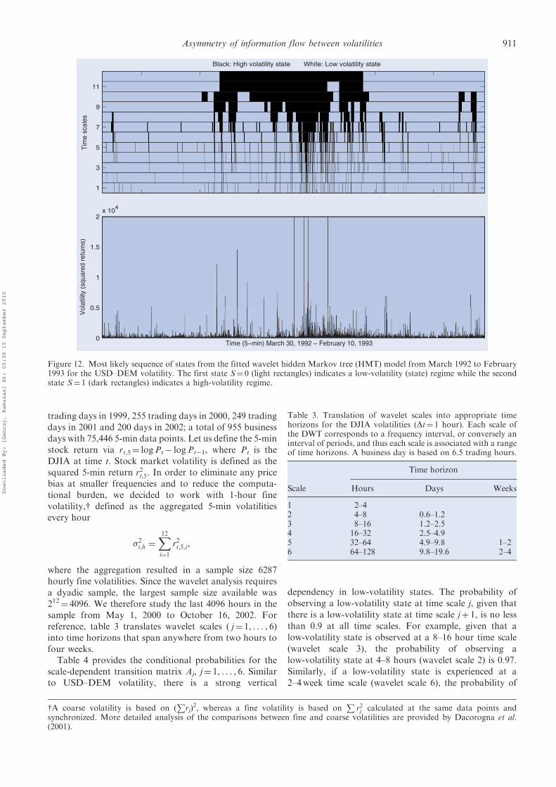
trading days in 1999, 255 trading days in 2000, 249 tradingdays in 2001 and 200 days in 2002; a total of 955 businessdays with 75,446 5-min data points. Let us define the 5-minstock return via rt,5¼ logPt� logPt�1, where Pt is theDJIA at time t. Stock market volatility is defined as thesquared 5-min return r2t,5. In order to eliminate any pricebias at smaller frequencies and to reduce the computa-tional burden, we decided to work with 1-hour finevolatility,y defined as the aggregated 5-min volatilitiesevery hour

�2t,h ¼X12i¼1

r2t,5,i,

where the aggregation resulted in a sample size 6287hourly fine volatilities. Since the wavelet analysis requiresa dyadic sample, the largest sample size available was212¼ 4096. We therefore study the last 4096 hours in thesample from May 1, 2000 to October 16, 2002. Forreference, table 3 translates wavelet scales ( j¼ 1, . . . , 6)into time horizons that span anywhere from two hours tofour weeks.

Table 4 provides the conditional probabilities for thescale-dependent transition matrix Aj, j¼ 1, . . . , 6. Similarto USD–DEM volatility, there is a strong vertical

dependency in low-volatility states. The probability ofobserving a low-volatility state at time scale j, given thatthere is a low-volatility state at time scale jþ 1, is no lessthan 0.9 at all time scales. For example, given that a

low-volatility state is observed at a 8–16 hour time scale(wavelet scale 3), the probability of observing alow-volatility state at 4–8 hours (wavelet scale 2) is 0.97.Similarly, if a low-volatility state is experienced at a

2–4week time scale (wavelet scale 6), the probability of

Black: High volatility state White: Low volatility state

Tim

e sc

ales

11

9

7

5

3

1

0

0.5

1

1.5

2x 104

Vol

atili

ty (

squa

red

retu

rns)

Time (5−min) March 30, 1992 − February 10, 1993

Figure 12. Most likely sequence of states from the fitted wavelet hidden Markov tree (HMT) model from March 1992 to February1993 for the USD–DEM volatility. The first state S¼ 0 (light rectangles) indicates a low-volatility (state) regime while the secondstate S¼ 1 (dark rectangles) indicates a high-volatility regime.

Table 3. Translation of wavelet scales into appropriate timehorizons for the DJIA volatilities (Dt¼ 1 hour). Each scale ofthe DWT corresponds to a frequency interval, or conversely aninterval of periods, and thus each scale is associated with a rangeof time horizons. A business day is based on 6.5 trading hours.

Time horizon

Scale Hours Days Weeks

1 2–42 4–8 0.6–1.23 8–16 1.2–2.54 16–32 2.5–4.95 32–64 4.9–9.8 1–26 64–128 9.8–19.6 2–4

yA coarse volatility is based on (P

rj)2, whereas a fine volatility is based on

Pr2j calculated at the same data points and

synchronized. More detailed analysis of the comparisons between fine and coarse volatilities are provided by Dacorogna et al.(2001).



observing a low-volatility state at 1–2 weeks (wavelet scale

5) is 0.90.y Technically, this means that given a waveletcoefficient associated with low volatility, there is very

little chance that it will produce a wavelet coefficient

associated with high volatility at the lower scale. Hence,

the conditional probabilities for low-to-low volatilitystates are 0.90 and larger. Naturally, the probability of

changing states (from low volatility at time scale j to high

volatility at time scale j� 1) is not greater than 0.10, as

presented in table 4. We conclude that vertical depen-

dency in low-volatility states is quite strong. Thesefindings are in line with those previously discussed for

FX volatility.The vertical dependency among high-volatility states is

not as strong as it is in low-volatility states, especially atlower time scales. This means that a high-volatility state

(regime) at a given time scale will not guarantee that

wavelet coefficients at the lower time scale will be

associated with high volatility. For example, given ahigh-volatility regime at a 8–16 hour time scale (wavelet

scale 3), the probability of being in a high-volatility

regime at 4–8 hours (wavelet scale 2) is 0.25. Similarly, if

a high-volatility regime prevails at a 2–4 week time scale

(wavelet scale 6), the probability of being in ahigh-volatility regime at 1–2 weeks (wavelet scale 5) is

just 0.17. The conditional probabilities for the

scale-dependent transition matrix of the stock market

volatility indicates that low-volatility stability is strongin the stock market. Contrary to the FX market, the

probability of changing states from a high to a low state is

much higher in the stock market, especially at higher

scales. For example, given a high-volatility state at a2–4week time scale (wavelet scale 6), the probability of

observing a low-volatility state at 1–2 weeks (wavelet scale

5) is 0.82. This indicates that switching to a low-volatility

state is more likely across scales in the stock market ascompared to the FX market(s).

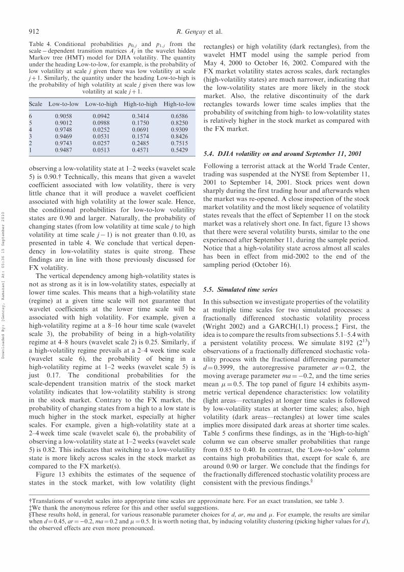
Figure 13 exhibits the estimates of the sequence of

states in the stock market, with low volatility (light

rectangles) or high volatility (dark rectangles), from thewavelet HMT model using the sample period fromMay 4, 2000 to October 16, 2002. Compared with theFX market volatility states across scales, dark rectangles(high-volatility states) are much narrower, indicating thatthe low-volatility states are more likely in the stockmarket. Also, the relative discontinuity of the darkrectangles towards lower time scales implies that theprobability of switching from high- to low-volatility statesis relatively higher in the stock market as compared withthe FX market.

5.4. DJIA volatility on and around September 11, 2001

Following a terrorist attack at the World Trade Center,trading was suspended at the NYSE from September 11,2001 to September 14, 2001. Stock prices went downsharply during the first trading hour and afterwards whenthe market was re-opened. A close inspection of the stockmarket volatility and the most likely sequence of volatilitystates reveals that the effect of September 11 on the stockmarket was a relatively short one. In fact, figure 13 showsthat there were several volatility bursts, similar to the oneexperienced after September 11, during the sample period.Notice that a high-volatility state across almost all scaleshas been in effect from mid-2002 to the end of thesampling period (October 16).

5.5. Simulated time series

In this subsection we investigate properties of the volatilityat multiple time scales for two simulated processes: afractionally differenced stochastic volatility process(Wright 2002) and a GARCH(1,1) process.z First, theidea is to compare the results from subsections 5.1–5.4 witha persistent volatility process. We simulate 8192 (213)observations of a fractionally differenced stochastic vola-tility process with the fractional differencing parameterd¼ 0.3999, the autoregressive parameter ar¼ 0.2, themoving average parameter ma¼�0.2, and the time seriesmean ¼ 0.5. The top panel of figure 14 exhibits asym-metric vertical dependence characteristics: low volatility(light areas—rectangles) at longer time scales is followedby low-volatility states at shorter time scales; also, highvolatility (dark areas—rectangles) at lower time scalesimplies more dissipated dark areas at shorter time scales.Table 5 confirms these findings, as in the ‘High-to-high’column we can observe smaller probabilities that rangefrom 0.85 to 0.40. In contrast, the ‘Low-to-low’ columncontains high probabilities that, except for scale 6, arearound 0.90 or larger. We conclude that the findings forthe fractionally differenced stochastic volatility process areconsistent with the previous findings.x

Table 4. Conditional probabilities p0, j and p1, j from thescale� dependent transition matrices Aj in the wavelet hiddenMarkov tree (HMT) model for DJIA volatility. The quantityunder the heading Low-to-low, for example, is the probability oflow volatility at scale j given there was low volatility at scalejþ 1. Similarly, the quantity under the heading Low-to-high isthe probability of high volatility at scale j given there was low


Scale Low-to-low Low-to-high High-to-high High-to-low

6 0.9058 0.0942 0.3414 0.65865 0.9012 0.0988 0.1750 0.82504 0.9748 0.0252 0.0691 0.93093 0.9469 0.0531 0.1574 0.84262 0.9743 0.0257 0.2485 0.75151 0.9487 0.0513 0.4571 0.5429

yTranslations of wavelet scales into appropriate time scales are approximate here. For an exact translation, see table 3.zWe thank the anonymous referee for this and other useful suggestions.xThese results hold, in general, for various reasonable parameter choices for d, ar, ma and . For example, the results are similarwhen d¼ 0.45, ar¼�0.2, ma¼ 0.2 and ¼ 0.5. It is worth noting that, by inducing volatility clustering (picking higher values for d ),the observed effects are even more pronounced.



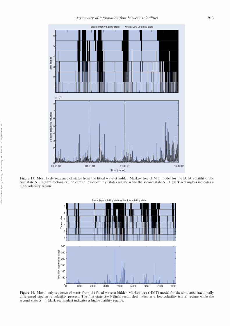
Black: High volatility state White: Low volatility state

Tim

e sc

ales

6

5

4

3

2

1

01.01.00 01.01.01 11.09.01 16.10.020

1

2

3

4

5

6

7

8

x 104

Time (hours)

Vol

atili

ty (

squa

red

retu

rns)

Figure 13. Most likely sequence of states from the fitted wavelet hidden Markov tree (HMT) model for the DJIA volatility. Thefirst state S¼ 0 (light rectangles) indicates a low-volatility (state) regime while the second state S¼ 1 (dark rectangles) indicates ahigh-volatility regime.

Black: high volatility state white: low volatility state

Tim

e sc

ales

6

5

4

3

2

1

0 1000 2000 3000 4000 5000 6000 7000 80000

50

100

150

200

250

300

Vol

atili

ty (

squa

red

retu

rns)

Figure 14. Most likely sequence of states from the fitted wavelet hidden Markov tree (HMT) model for the simulated fractionallydifferenced stochastic volatility process. The first state S¼ 0 (light rectangles) indicates a low-volatility (state) regime while thesecond state S¼ 1 (dark rectangles) indicates a high-volatility regime.



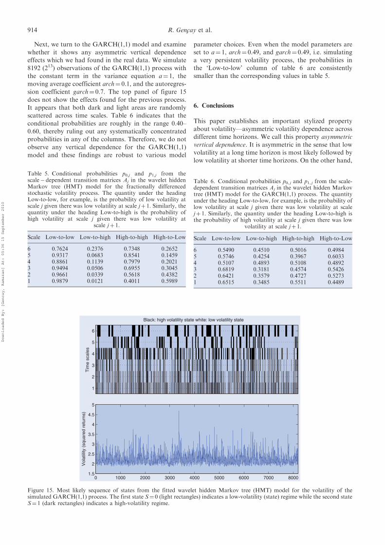
Next, we turn to the GARCH(1,1) model and examine

whether it shows any asymmetric vertical dependence

effects which we had found in the real data. We simulate

8192 (213) observations of the GARCH(1,1) process with

the constant term in the variance equation a¼ 1, the

moving average coefficient arch¼ 0.1, and the autoregres-

sion coefficient garch¼ 0.7. The top panel of figure 15

does not show the effects found for the previous process.

It appears that both dark and light areas are randomly

scattered across time scales. Table 6 indicates that the

conditional probabilities are roughly in the range 0.40–

0.60, thereby ruling out any systematically concentrated

probabilities in any of the columns. Therefore, we do not

observe any vertical dependence for the GARCH(1,1)

model and these findings are robust to various model

parameter choices. Even when the model parameters areset to a¼ 1, arch¼ 0.49, and garch¼ 0.49, i.e. simulating

a very persistent volatility process, the probabilities inthe ‘Low-to-low’ column of table 6 are consistently

smaller than the corresponding values in table 5.

6. Conclusions

This paper establishes an important stylized propertyabout volatility—asymmetric volatility dependence across

different time horizons. We call this property asymmetricvertical dependence. It is asymmetric in the sense that low

volatility at a long time horizon is most likely followed bylow volatility at shorter time horizons. On the other hand,

Table 5. Conditional probabilities p0,j and p1,j from thescale� dependent transition matrices Aj in the wavelet hiddenMarkov tree (HMT) model for the fractionally differencedstochastic volatility process. The quantity under the headingLow-to-low, for example, is the probability of low volatility atscale j given there was low volatility at scale jþ 1. Similarly, thequantity under the heading Low-to-high is the probability ofhigh volatility at scale j given there was low volatility at

scale jþ 1.

Scale Low-to-low Low-to-high High-to-high High-to-Low

6 0.7624 0.2376 0.7348 0.26525 0.9317 0.0683 0.8541 0.14594 0.8861 0.1139 0.7979 0.20213 0.9494 0.0506 0.6955 0.30452 0.9661 0.0339 0.5618 0.43821 0.9879 0.0121 0.4011 0.5989

Black: high volatility state white: low volatility state

Tim

e sc

ales

6

5

4

3

2

1

0 1000 2000 3000 4000 5000 6000 7000 80001.5

2

2.5

3

3.5

4

4.5

5

Vol

atili

ty (

squa

red

retu

rns)

Figure 15. Most likely sequence of states from the fitted wavelet hidden Markov tree (HMT) model for the volatility of thesimulated GARCH(1,1) process. The first state S¼ 0 (light rectangles) indicates a low-volatility (state) regime while the second stateS¼ 1 (dark rectangles) indicates a high-volatility regime.

Table 6. Conditional probabilities p0, j and p1, j from the scale-dependent transition matrices Aj in the wavelet hidden Markovtree (HMT) model for the GARCH(1,1) process. The quantityunder the heading Low-to-low, for example, is the probability oflow volatility at scale j given there was low volatility at scalejþ 1. Similarly, the quantity under the heading Low-to-high isthe probability of high volatility at scale j given there was low


Scale Low-to-low Low-to-high High-to-high High-to-Low

6 0.5490 0.4510 0.5016 0.49845 0.5746 0.4254 0.3967 0.60334 0.5107 0.4893 0.5108 0.48923 0.6819 0.3181 0.4574 0.54262 0.6421 0.3579 0.4727 0.52731 0.6515 0.3485 0.5511 0.4489



high volatility at long time horizons does not necessarilyimply high volatility at shorter time horizons.

Our analysis provides evidence that volatility may bemodeled as a mixture of high- and low-volatility regimes,resulting in a mixture distribution that is non-Gaussian.This result has important implications regarding thescaling behavior of volatility, and also for the calculationof risk at different time horizons. Our approach, usingwavelet-based hidden Markov models for time seriesanalysis, shows great promise in succinctly capturing thenon-Gaussian features found in high-frequency FX ratesby simultaneously modeling multiple time horizons.Although we focused our attention on the wavelethidden Markov tree (HMT) model, another possiblemodel is to allow dependence within and between scalesthrough hidden Markov chains and hidden Markov trees.In addition to taking advantage of the persistence acrossscales, this would allow us to explicitly model volatilityclustering in time.

Acknowledgements

Ramo Gencay gratefully acknowledges financial supportfrom the Natural Sciences and Engineering ResearchCouncil of Canada, the Social Sciences and HumanitiesResearch Council of Canada. We are grateful to OlsenGroup (www.olsen.ch), Switzerland, for providing thedata, and Dr. Richard Baraniuk for providing some of thewavelet software used in this paper. The software and dataused in this paper are available at www.sfu.ca/rgencay.

References

Andersen, T.G., Bollerslev, T., Diebold, F.X. and Labys, P.,The distribution of realized exchange rate volatility. J. Am.Statist. Assoc., 2001, 96, 42–55.

Baum, L., An inequality and associated maximization techniquein statistical estimation of probabilistic functions of Markovprocesses. Inequalities, 1972, 3, 1–8.

Bollerslev, T., Generalized autoregressive conditional hetero-skedasticity. J. Econometr., 1986, 31, 307–327.

Borland, L., Bouchaud, J.-P., Muzy, J.-F. and Zumbach, G.,The dynamics of financial markets—Mandelbrot’s multi-fractal cascades, and beyond. Working Paper, 2008 (Science &Finance (CFM) working paper archive (500061)).

Calvet, L. and Fisher, A., Multifractality in asset returns: theoryand evidence. Rev. Econ. Statist., 2002, 84, 381–406.

Crouse, M.S., Nowak, R.D. and Baraniuk, R.G., Wavelet-basedstatistical signal processing using hidden Markov models.IEEE Trans. Signal Process., 1998, 46, 886–902.

Dacorogna, M., Gencay, R., Muller, U., Pictet, O. andOlsen, R., An Introduction to High-Frequency Finance, 2001(Academic Press: San Diego).

Durand, J.-B. and Goncalves, P., Statistical inference for hiddenMarkov tree models and application to wavelet trees.Technical Report 4248, Statistical Inference for Industryand Health, INRIA, 2001.

Engle, R.F., Autoregressive conditional heteroskedasticity withestimates of the variance of U.K. inflation. Econometrica,1982, 50, 987–1008.

Fung, W. and Hsieh, D.A., Measuring the market impact ofhedge funds. J. Empir. Finance, 2000, 7, 1–36.

Gencay, R., Ballocchi, G., Dacorogna, M., Olsen, R.B. andPictet, O.V., Real-time trading models and the statisticalproperties of foreign exchange rates. Int. Econ. Rev., 2002, 43,463–491.

Gencay, R., Dacorogna, M., Olsen, R.B. and Pictet, O.V., Real-time foreign exchange trading models and market behavior.J. Econ. Dynam. Control, 2003, 27, 909–935.

Gencay, R., Selcuk, F. and Whitcher, B., Differentiatingintraday seasonalities through wavelet multi-scaling. PhysicaA, 2001a, 289, 543–556.

Gencay, R., Selcuk, F. and Whitcher, B., An Introduction toWavelets and Other Filtering Methods in Finance andEconomics, 2001b (Academic Press: San Diego).

Gencay, R., Selcuk, F. and Whitcher, B., Scalingproperties of foreign exchange volatility. Physica A, 2001c,289, 89–106.

Ghysels, E., Santa-Clara, P. and Valkanov, R., Predictingvolatility: how to get the most out of returns data sampled atdifferent frequencies. J. Econometr., 2006, 131, 59–95.

Hamilton, J.D., A new approach to the economic analysis ofnonstationary time series and the business cycle.Econometrica, 1989, 57, 357–384.

Maheu, J.M. and McCurdy, T.H., Nonlinear features of realizedFX volatility. Rev. Econ. Statist., 2002, 84, 1–24.

Mallat, S., AWavelet Tour of Signal Processing, 1998 (AcademicPress: San Diego).

Mandelbrot, B.B., The variation of certain speculative prices.J. Business, 1963, 36, 394–419.

Mandelbrot, B.B., When can price be arbitraged efficiently?A limit to the validity of the random walk and martingalemodel. Rev. Econ. Statist., 1971, 53, 225–236.

Muller, U.A., Dacorogna, M.M., Dave, R.D., Olsen, R.B.,Pictet, O.V. and von Weizsacker, J.E., Volatilities of differenttime resolutions – analyzing the dynamics of marketcomponents. J. Empir. Finance, 1997, 4, 213–239.

Percival, D.B. and Walden, A.T., Wavelet Methods for TimeSeries Analysis, 2000 (Cambridge University Press:Cambridge).

Rabiner, L.R., A tutorial on hidden Markov models andselected applications in speech recognition. Proc. IEEE, 1989,77, 257–286.

Ramsey, J.B., Wavelets in economics and finance: past andfuture. Stud. Nonlinear Dynam. Econ., 2002, 6, Article 1.

Smyth, P., Heckerman, D. and Jordan, M.I., Probabilisticindependence networks for hidden Markov probabilitymodels. Neural Comput., 1996, 9, 227–269.

Weber, P., Wang, F., Vodenska-Chitkushev, I., Havlin, S. andStanley, H.E., Relation between volatility correlations infinancial markets and Omori processes occurring on all scales.Phys. Rev. E, 2007, 76, 1–8.

Wright, J.H., Log-periodogram estimation of long memoryvolatility dependencies with conditionally heavy tailedreturns. Econometr. Rev., 2002, 21, 397–417.

Zumbach, G., Volatility processes and volatility forecast withlong memory. Quant. Finance, 2004, 4, 70–86.

Zumbach, G., Time reversal invariance in finance. Workingpaper, 2007. Available online at: SSRN: http://ssrn.com/abstract=1004992

Zumbach, G. and Lynch, P., Heterogeneous volatility cascade infinancial markets. Physica A, 2001, 298, 521–529.



Documents

Asymmetry of information flow between volatilities across ...rgencay/jarticles/qf-hmm.pdf · Asymmetry of information flow between volatilities across time ... model regimes of volatilities