Asymptotic distribution of entry times in a cellular

automaton with annihilating particles

Petr Kurka, Enrico Formenti, Alberto Dennunzio

To cite this version:

Petr Kurka, Enrico Formenti, Alberto Dennunzio. Asymptotic distribution of entry timesin a cellular automaton with annihilating particles. Fates, Nazim and Goles, Eric and Maass,Alejandro and Rapaport, Ivan. 17th International Workshop on Celular Automata and DiscreteComplex Systems, 2011, Santiago, Chile. Discrete Mathematics and Theoretical ComputerScience, AP, pp.47-58, 2012, DMTCS Proceedings. <hal-01196143>

HAL Id: hal-01196143

https://hal.inria.fr/hal-01196143

Submitted on 9 Sep 2015

HAL is a multi-disciplinary open accessarchive for the deposit and dissemination of sci-entific research documents, whether they are pub-lished or not. The documents may come fromteaching and research institutions in France orabroad, or from public or private research centers.

L’archive ouverte pluridisciplinaire HAL, estdestinee au depot et a la diffusion de documentsscientifiques de niveau recherche, publies ou non,emanant des etablissements d’enseignement et derecherche francais ou etrangers, des laboratoirespublics ou prives.

brought to you by COREView metadata, citation and similar papers at core.ac.uk

provided by HAL-UNICE

AUTOMATA 2011, Santiago, Chile DMTCS proc. AP, 2012, 47–58

Asymptotic distribution of entry times in acellular automaton with annihilating particles

Petr Kurka1† Enrico Formenti2‡¶ Alberto Dennunzio23§¶

1Center for Theoretical Study, Academy of Sciences and Charles University in Prague, Czechia2Laboratoire I3S, Universite Nice Sophia Antipolis, France3Dipartimento di Informatica, Sistemistica e Comunicazione, Universita degli Studi di Milano–Bicocca, Italy

This work considers a cellular automaton (CA) with two particles: a stationary particle 1 and left-going one 1. Whena 1 encounters a 1, both particles annihilate. We derive asymptotic distribution of appearence of particles at a givensite when the CA is initialized with the Bernoulli measure with the probabilities of both particles equal to 1/2.

Keywords: Cellular Automata, Particle Systems, Entry Times, Return Times

1 IntroductionCellular automata are a simple formal model for complex systems. They consist of an infinite numberof identical finite automata arranged over a regular lattice (here Z). Each automaton updates its stateaccording to its own state and the one of a fixed set of neighboring automata according to a local rule. Allupdates are synchronous.

The simplicity of the model contrasts with the great variety of different dynamical behaviors. Indeed,exactly this rich variety of behaviors and the ease of being simulated on computers made CA fortune.Actually, they are used in almost all scientific disciplines ranging from Mathematics to Computer Scienceand Natural Sciences. In particular, in Biology, Physics and Economics, they can be used as a discretecounterpart (in the sense of time) of interacting particle systems (IPS).

The advantage of modeling IPS by CA is that one can have information not only about limit distributionsand particle densities but also on their spatial distribution.

On the other hand, as we have already mentioned, the dynamical behavior of CA is complex and notfully understood and IPS can help to understand the dynamics of some CA whenever it can be describedin terms of particles or signals that move in a neutral background and interact on encounters. The generalconcept of a signal or particle (in the context of CA) has been elaborated in Formenti and Kurka (2007).

†Email: kurka@cts.cuni.cz. This research was supported by the Research Program CTS MSM 0021620845‡Email: enrico.formenti@unice.fr§Email: dennunzio@disco.unimib.it¶Supported by the French National Research Agency project EMC (ANR-09-BLAN-0164)

1365–8050 c© 2012 Discrete Mathematics and Theoretical Computer Science (DMTCS), Nancy, France

48 Petr Kurka, Enrico Formenti, Alberto Dennunzio

The simplest kind of particles interaction is the annihilation. The classical example is “Just gliders”studied in Gilman (1987). This system consists of a left-going particle 1 and a right-going particle 1which annihilate on encounters. If the system starts in a Bernoulli measure with equal probabilities ofboth particles, then at a specified site both kinds of particles keep appearing with probability one, althoughtheir appearance is more and more rare as it has been shown by Kurka and Maass (2002). Other peculiarparticle systems and related CA models have been studied, see for example Fisch (1990).

In the present paper we address the question of how the time of appearance of a particle dependson the age of the system. We work with a simpler system called asymmetric gliders consisting of onestationary and one left-going particles annihilating on encounters. We show that the appearance of left-going particles time scales linearly with the age of the system and we derive the limit scaled distribution.

The paper is organized as follows. Section 2 and 3 introduce the symmetric and asymmetric glidersCA, respectively. Results are in Section 3. Since the proofs of the main results require several technicallemmata and specific notations, we grouped them in Section 4. The final section draws some conclusionsand give some ideas for future work.

2 Symmetric glidersLet A be a finite alphabet. A 1D CA configuration is a function from Z to A. The 1D CA configurationset AZ is usually equipped with the metric d defined as follows

∀c, c′ ∈ AZ, d(c, c′) = 2−n, where n = min{i ≥ 0 : ci 6= c′i or c′−i 6= c′−i

}.

If A is finite, AZ is a compact, totally disconnected and perfect topological space (i.e., AZ is a Cantorspace). For any pair i, j ∈ Z, with i ≤ j, and any configuration x ∈ AZ we denote by x[i,j] the wordxi · · ·xj ∈ Aj−i+1, i.e., the portion of c inside the interval [i, j]. In the previous notation, [i, j] can bereplaced by [i, j) with the obvious meaning. A cylinder of block u ∈ Ak and position i ∈ Z is the set[u]i = {x ∈ AZ : x[i,i+k−1] = u}. Cylinders are clopen sets w.r.t. the metric d and they form a basis forthe topology induced by d.

A 1D CA is a structure 〈1, A, r, f〉, where A is the alphabet, r ∈ N is the radius and f : A2r+1 → A isthe local rule of the automaton. The local rule f induces a global rule F : AZ → AZ defined as follows,

∀c ∈ AZ, ∀i ∈ Z, F (c)i = f(ci−r, . . . , ci, . . . , ci+r) .

In Gilman (1987), Gilman introduced a CA called Just Gliders (or Symmetric Gliders) which is formallydefined as 〈1,

{1, 0, 1

}, 1, g〉 where g :

{1, 0, 1

}3 → {1, 0, 1

}is such that

∀(x, y, z) ∈{

1, 0, 1}3, g(x, y, z) =

1 if x = 1, y ≥ 0 and y + z ≥ 01 if z = 1, y ≤ 0 and x+ y ≤ 00 otherwise .

In this context a symbol 1 (resp. 1) is interpreted as a right-going (resp. left-going) particle and 0 isthe neutral background. Figure 1 shows an example of evolution of Just Gliders from a random initialconfiguration.

Asymptotic distribution of entry times in cellular automata 49

Fig. 1: Symmetric gliders.

Consider a Bernoulli measure on{

1, 0, 1}Z

, i.e., a sequence of independent identically distributedrandom variables X = (Xi)i∈Z over

{1, 0, 1

}such that ∀i ∈ Z,P[Xi = 1] = P[Xi = 1] = p, P[Xi =

0] = 1 − 2p = q. Then, for any CA global rule F and any n ∈ N, Fn(X)0 is also a random variablewhose distribution depends on the initial distribution of X .

Definition 1 (Entry time) For a ∈{

1, 0, 1}

, the entry time into [a]0 (appearance of a particle a) aftertime n at position 0 is

T an (X) = min

{k ≥ 0 : Fn+k(X)0 = a

}.

Since F commutes with σ, the entry times at any position s ∈ Z have the same distribution as T an .

In Gilman (1987), the following result has been proven.

Theorem 1 Let F be the global function of Just Gliders CA. If P[Xi = 1] > P[Xi = 1] then

P[∀n ∈ N,∃k ∈ N s.t. Fn+k(X)0 = 1] = P[∀n ∈ N, T 1n(X) <∞] = 0 .

Then Kurka and Maass (2002) proved the following

Theorem 2 Let F be the global function of Just Gliders CA. If P[Xi = 1] = P[Xi = 1] then

1. P[∀n ∈ N,∃k ∈ N s.t. Fn+k(X)0 6= 0] = 1;

2. P[∀n ∈ N, T an (X) <∞] = 1 for a ∈

{1, 1}

;

3. ∀n ∈ N, P[T an (X) <∞] = 1 for a ∈

{1, 1}

;

4. limn→∞ P[Fn(X)0 = 0] = 1.

3 Asymmetric glidersIn this paper we consider a similar CA that we call Asymmetric Gliders, 〈1,

{1, 0, 1

}, 1, f〉 and f :{

1, 0, 1}3 → {

1, 0, 1}

is defined as follows

∀(x, y, z) ∈{

1, 0, 1}3, f(x, y, z) =

1 if y = 1 and z 6= 11 if y 6= 1 and z = 10 otherwise .

50 Petr Kurka, Enrico Formenti, Alberto Dennunzio

Fig. 2: Asymmetric gliders.

The symbol 1 can be interpreted as a stationary particle, 1 is a left-going particle and 0 is the neutralbackground. It is clear from the definition of f that a particle 1 and a 1 annihilate when they meet (Figure2). In the sequel, the symbols of A are weighted naturally, namely, 0 with 0, 1 with 1 and 1 with −1.Thus, for example, 1 + 1 = 0 and 1 + 1 = −2 and so on.

Again, we consider a Bernoulli measure on{

1, 0, 1}Z

, i.e., a sequence of independent identically dis-tributed random variables X = (Xi)i∈Z over

{1, 0, 1

}such that ∀i ∈ Z,P[Xi = 1] = P[Xi = 1] = p,

P[Xi = 0] = 1 − 2p = q. Then, for any CA global rule F and any n ∈ N, Fn(X)0 is also a randomvariable whose distribution depends on the initial distribution of X .

Proposition 1 Let F be the global function of Asymmetric Gliders CA. If ∀i ∈ Z, P[Xi = 1] = P[Xi =1] ≤ 1/2 then

1. limn→∞ P[Fn(X)0 = 0] = 1;

2. limn→∞ P[T 0n(X) = 0] = 1;

3. limn→∞ P[T 1n(X) =∞] = 1.

Proof: The following relations between Fn(X)0 and the random variables Xi hold

Fn(X)0 = 1 ⇔ ∀k ≤ n,k∑

i=0

Xi > 0

Fn(X)0 = 1 ⇔ ∀k ≤ n,n∑

i=k

Xi < 0

Fn(X)0 = 0 ⇔ ∃k ≤ n,k∑

i=0

Xi ≤ 0 and ∃k ≤ n,n∑

i=k

Xi ≥ 0

Since∑n

i=0Xi is a recurrent Markov chain, we get

limn→∞

P[Fn(X)0 = 1] = limn→∞

P[Fn(X)0 = 1] = 0

Asymptotic distribution of entry times in cellular automata 51

Therefore, it follows that limn→∞ P[Fn(X)0 = 0] = 1, limn→∞ P[T 0n(X) = 0] = 1, and also

limn→∞ P[T 1n(X) =∞] = 1. 2

As a consequence of Proposition 1 as n → ∞, T 0n(X) → 0 and T 1

n(X) → ∞ in probability. More-over, since for any n ∈ N the set of events such that T 1

n(X) = ∞ is contained in the one such thatlimn→∞ T 1

n(X) = ∞, it holds that P[limn→∞ T 1n(X) = ∞] ≥ limn→∞ P[T 1

n(X) = ∞] = 1, and,hence, T 1

n(X)→∞ almost surely.

Proposition 2 Let F be the global function of Asymmetric Gliders CA. If ∀i ∈ Z, P[Xi = 1] = P[Xi =1] = 1/2 then

1. ∀x, limn→∞ P[T 1n(X) > x] = 1;

2. ∀n ∈ N, E(T 1n) =∞.

Theorem 3 Let F be the global function of Asymmetric Gliders CA. If ∀i ∈ Z, P[Xi = 1] = P[Xi =1] = 1/2 then

limn→∞

P

[T 1n(X)

n≤ x

]=

2

πarctan

√x .

In the general case with p ≤ 1/2 we have Var(X) = 2p so the time scales by√

2p. Hence, we cangive the following.

Conjecture 1 Let F be the global function of Asymmetric Gliders CA. If ∀i ∈ Z, P[Xi = 1] = P[Xi =1] ≤ 1/2 then

limn→∞

P

[T 1n(X)

n≤ x

]=

2

πarctan

√2px .

4 Proof of main resultsNotation. For the sake of simplicity, from now on T 1

n is denoted Tn whenever no misunderstanding ispossible.

First of all, we should precise the definition of what we mean by annihilation of particles 1 and 1.

Definition 2 (Annihilation) A particle 1 at the position n is annihilated with the particle 1 at positionn+ k, if F k−1(X)n = 1 and F k−1(X)n+1 = 1.

Denote by Yn the number of particles 1 in the interval [0, n) which are not annihilated with any particle1 in the interval [0, n). Then, Y0 = 0 and Yn+1 = max{0, Yn + Xn}, so Y is a Markov chain whosetransition probabilities are in Figure 3.

For the probabilities Pn,m = P[Yn = m] we have P0,0 = 1 and Pn,m = 0 for m > n. The balanceequations for the Markov chain Y give

Pn+1,0 = (1− p) · Pn,0 + p · Pn,1 (1)Pn+1,m = p · Pn,m−1 + (1− 2p) · Pn,m + p · Pn,m+1 for m > 0 (2)

52 Petr Kurka, Enrico Formenti, Alberto Dennunzio

0 1 2 . . .

1-p

p

p

1-2p

p

p

1-2p

p

p

Fig. 3: The Markov chain Y above defined.

For a fixed n ≥ 0 consider the stochastic process Z such that Z0 = Yn and Zm+1 = Zm + Xn+m. IfZ0, . . . Zm are all nonnegative, thenZm is the number of particles 1 in [0, n+m) which are not annihilatedwith any particle 1 in [0, n+m). For m ≥ l define the entry times for Z as follows

Sm,l = min{t > 0 : Zt = l|Z0 = m}

and the associated probabilities

Qm,k = P[Sm+l,l = k] = P[Sm,0 = k] .

Remark that for m2 > m1 > m0 we have Sm2,m0 = Sm2,m1 + Sm1,m0 , so Sm,0 is the sum of mindependent random variables which have all the same distribution as S1,0. Thus Q0,1 = q, Q0,2 = 2p2,Q1,1 = p,Qm,1 = 0 form > 1,Q1,2 = p(1−2p) = pq,Q2,2 = p2 andQm,k = 0 form > k. Accordingto the equilibrium equation of the Markov chain Z one finds

Q0,k+1 = 2p ·Q1,k for m = 0 (3)Q1,k+1 = q ·Q1,k + p ·Q2,k for m = 1 (4)Qm,k+1 = p ·Qm−1,k + q ·Qm,k + p ·Qm+1,k for m > 1 (5)

0 1 . . .-1. . .

1-2p

p

p

1-2p

p

pp

p

1-2p

p

p

Fig. 4: The Markov chain Z above introduced.

Remark that Tn = k iff Zk+1 = −1 and Zj ≥ 0 for all j ≤ k. Thus, if Z0 = m, then Tn = kiff Sm,−1 = k + 1. So, for the entry time Tn and the related probabilities P[Tn = k|Z0 = m] andRn,k := P[Tn = k], we have

Tn = χ[Yn=m] · Sm,−1

P[Tn = k|Z0 = m] = P[Sm,−1 = k + 1] = Qm+1,k+1

Rn,k = P[Tn = k] =

min(n,k+1)∑m=0

Pn,m ·Qm+1,k+1

Asymptotic distribution of entry times in cellular automata 53

When ∀i ∈ Z, P[Xi = 1] = P[Xi = 1] = 1/2 and P[Xi = 0] = 0 from the definitions of theprobabilities P and Q we obtain the following matrices.

P =

0 1 2 3 4 · · ·0 1 0 0 0 0 · · ·1 1

212 0 0 0 · · ·

2 24

14

14 0 0 · · ·

3 38

38

18

18 0 · · ·

4 616

416

416

116

116 · · ·

......

......

......

. . .

Q =

1 2 3 4 5 6 7 · · ·0 0 1

2 0 18 0 1

16 0 · · ·1 1

2 0 18 0 1

16 0 5128 · · ·

2 0 14 0 1

8 0 564 0 · · ·

3 0 0 18 0 3

32 0 9128 · · ·

4 0 0 0 116 0 1

16 0 · · ·...

......

......

......

.... . .

Next lemmata will give closed formulas for P and Q.

Lemma 1 If ∀i ∈ Z, P[Xi = 1] = P[Xi = 1] = 1/2 then for all n,m ∈ N with m ≤ n, the followingequalities hold on the probabilities Pn,m:

P2n,2m+2 = P2n,2m+1 =

(2n

n+m+ 1

)· 2−2n (6)

P2n+1,2m = P2n+1,2m+1 =

(2n+ 1

n+m+ 1

)· 2−2n−1 (7)

Pn,m =

(n

dn+m2 e

)· 2−n (8)

Proof: We have P0,0 = 1. By induction, assume that equalities (6) and (7) are true for some valuen and for all m ≤ n. Since from equations (1) and (2), Pn+1,0 = (Pn,0 + Pn,1)/2 and Pn+1,m =(Pn,m−1 + Pn,m+1)/2, it follows that (6) and (7) are true for n + 1 and for all m ≤ n + 1. Thus, (6)and (7) hold, and, as a consequence, equality (8) too. 2

According to Renyi (1970), the following relation holds for the Qm,k

Q1,2k−1 = Q0,2k =1

k · 22k−1

(2k − 2k − 1

)= (−1)k−1 ·

(1/2k

)(9)

Lemma 2 If ∀i ∈ Z, P[Xi = 1] = P[Xi = 1] = 1/2 then for all m with 0 < m ≤ k the followingequalities on the quantities Qm,k hold.

Qm,k = 0, if mod2(k +m) = 1 (10)

while

Q2m,2k =m

k

(2k

k −m

)· 2−2k (11)

Q2m+1,2k+1 =2m+ 1

2k + 1

(2k + 1k −m

)· 2−2k−1 (12)

Qm,k =m

k

(k

(k −m)/2

)· 2−k, (13)

if mod2(k +m) = 0, where mod2(m) is m mod 2.

54 Petr Kurka, Enrico Formenti, Alberto Dennunzio

Proof: Since q = 0, if mod2(k + m) = 1 Equality (10) follows from the definition of Qm,k. Using thatQ2,k = 2 ·Q1,k+1, Qm+1,k = 2 ·Qm,k+1 −Qm−1,k (for m ≥ 1), and Equation (9), Equalities from (11)to (13), are true for Q1,k and Q2,k. The thesis is obtained by proceeding by finite induction on m. 2

Using the expressions found in Lemmata 1 and 2 and substituting them in the definition of Rn,k =P[Tn = k], one can easily find the following.

R2n,2k = 2−2n−2k−1min(n,k)∑

m=0

(2n

n+m

)(2k + 1k −m

)2m+ 1

2k + 1

R2n,2k+1 = 2−2n−2k−2min(n,k)∑

m=0

(2n

n+m+ 1

)(2k + 2k −m

)m+ 1

k + 1

R2n+1,2k = 2−2n−2k−2min(n,k)∑

m=0

(2n+ 1

n+m+ 1

)(2k + 1k −m

)2m+ 1

2k + 1

R2n+1,2k+1 = 2−2n−2k−3min(n,k)∑

m=0

(2n+ 1

n+m+ 1

)(2k + 2k −m

)m+ 1

k + 1

which can be summed up as follows

Rn,k = 2−n−k−1min(bn2 c,b

k2 c)∑

m=0

(n

bn2 c+m+ `n,k

)(k + 1bk2 c −m

)2m+ 1 + mod2(k)

k + 1

where `n,k = max{mod2(n),mod2(k)}.Finally, we will use the following approximation formula of binomial distribution by the normal distri-

bution.

Theorem 4 (Renyi (1970)) Let kn be a sequence of positive integers such that |2kn − n| < a√n for

some constant a. Then (nkn

)=

2n+1 · e−(2kn−n)2/2n√

2πn(1 +O(1/n))

and the constant in the remainder O(1/n) depends only on a.

Proof of Proposition 2:

1. Using the approximation given by Theorem 4 one finds

limn→∞

Pn,m = limn→∞

2e−m2/2n

√2πn

= 0

and hence

limn→∞

P[Tn ≤ `] = limn→∞

∑k=0

min(n,k)∑m=0

Pn,m ·Qm+1,k+1 = 0

Asymptotic distribution of entry times in cellular automata 55

2. To prove E(Tn) = ∞ we prove first that E(Sm,1) = ∞ for each m. Again, using Theorem 4, onefinds

Qm,k =m

k·(

kdk−m2 e

)· 2−k ≈ m

k· 2k+1 e

−m2

2k

√2πk

· 2−k =2m · e−m2

2k

k√

2πk(14)

whenever m <√k and mod2(k +m) = 0. For each ` we then have

E(Sm,0) =

∞∑k=1

k ·Qm,k ≥∞∑k=`

2m · e−m2

2k

√2πk

=∞ . (15)

Since E(Tn) is a finite linear combination of E(S0,−1), . . . ,E(Sn,−1), we get E(Tn) =∞ as well.

2

Proof of Theorem 3: Recall that the characteristic function of a discrete distribution with P[X = n] = pnis ϕ(t) =

∑∞n=0 pne

int, where i is the imaginary unit. Since by Lemma 2Qm,k = 0 if mod2(k+m) = 1,for the characteristic function ϕ of S1,0 we obtain

ϕ(t) = Q1,1eit +Q1,3e

3it +Q1,5e5it + · · ·

which, by using Equation (9), turns into

ϕ(t) =

(1/21

)eit −

(1/22

)e3it +

(1/23

)e5it − · · ·

= e−it[1−

(1−

(1/21

)e2it +

(1/22

)e4it − · · ·

)]= e−it(1−

√1− e2it) .

Thus, finally we get

limn→∞

ϕ

(t

n2

)n

= limn→∞

(1−√

1− e2it/n2)n = limn→∞

(1−√−2it

n

)n

= e−√−2it

which is the characteristic function of a random variable with distribution function

G(x) = 2(1− Φ(1/√x))

and density

g(x) = G′(x) =1√

2πx3· e−1/2x ,

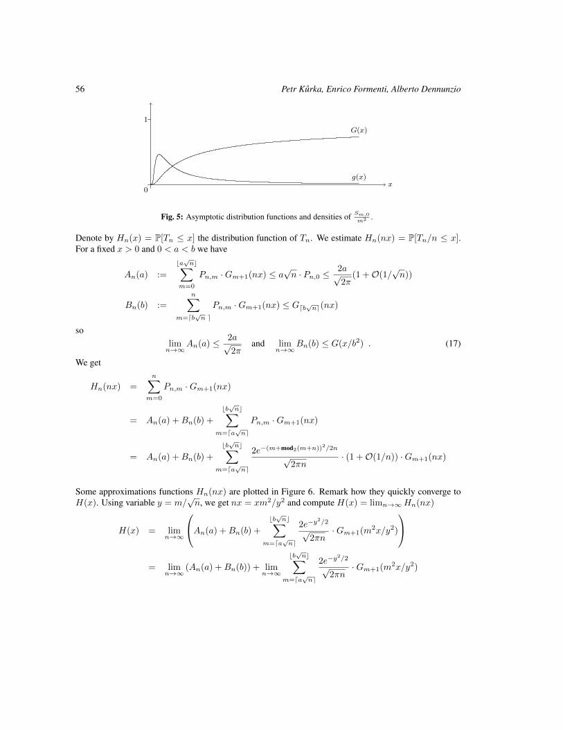
where Φ(x) is the normal distribution function. Figure 5 plots both G(x) and g(x).Recall that E(Sm,0) = ∞ (see Equation 15). Denote by Gm(x) = P[Sm,0 ≤ x] the distribution

function of Sm,0. Since the characteristic function of Sm,0 is ϕm(t) = ϕ(t)m, we get

limm→∞

Gm+1(m2x) = limm→∞

P[Sm,−1

m2< x

]= G(x) = 2(1− Φ(1/

√x)) (16)

56 Petr Kurka, Enrico Formenti, Alberto Dennunzio

1

0x

g(x)

G(x)

Fig. 5: Asymptotic distribution functions and densities of Sm,0

m2 .

Denote by Hn(x) = P[Tn ≤ x] the distribution function of Tn. We estimate Hn(nx) = P[Tn/n ≤ x].For a fixed x > 0 and 0 < a < b we have

An(a) :=

ba√nc∑

m=0

Pn,m ·Gm+1(nx) ≤ a√n · Pn,0 ≤

2a√2π

(1 +O(1/√n))

Bn(b) :=

n∑m=db

√n e

Pn,m ·Gm+1(nx) ≤ Gdb√ne(nx)

solimn→∞

An(a) ≤ 2a√2π

and limn→∞

Bn(b) ≤ G(x/b2) . (17)

We get

Hn(nx) =

n∑m=0

Pn,m ·Gm+1(nx)

= An(a) +Bn(b) +

bb√nc∑

m=da√ne

Pn,m ·Gm+1(nx)

= An(a) +Bn(b) +

bb√nc∑

m=da√ne

2e−(m+mod2(m+n))2/2n

√2πn

· (1 +O(1/n)) ·Gm+1(nx)

Some approximations functions Hn(nx) are plotted in Figure 6. Remark how they quickly converge toH(x). Using variable y = m/

√n, we get nx = xm2/y2 and compute H(x) = limn→∞Hn(nx)

H(x) = limn→∞

An(a) +Bn(b) +

bb√nc∑

m=da√ne

2e−y2/2

√2πn

·Gm+1(m2x/y2)

= lim

n→∞(An(a) +Bn(b)) + lim

n→∞

bb√nc∑

m=da√ne

2e−y2/2

√2πn

·Gm+1(m2x/y2)

Asymptotic distribution of entry times in cellular automata 57

1

0x

H(x)

h(x)

H2(2x)

H10(10x)

Fig. 6: Asymptotic distribution functions and densities of Tnn

.

and, by using 16, we obtain (recall that y = m/√n ∈ [a, b])

H(x) = limn→∞

(An(a) +Bn(b)) +

√2

π

b∑y=a

e−y2/2 ·Gm+1(m2x/y2)

Since lima→0

limn→∞

An(a) = 0 and limb→∞

limn→∞

Bn(b) = 0 (see Inequalities in 17), we have

H(x) =

√2

π· lima→0

limb→∞

b∑y=a

e−y2/2 ·Gm+1(m2x/y2)

=

√2

π

∫ ∞0

e−y2/2 ·G(x/y2) dy

which gives for the density

h(x) = H′(x) =

√2

π·∫ ∞0

e−y2/2 · g(x/y2) · y−2 dy

=1

π√x3

∫ ∞0

y · e−y2

2 (1+ 1x ) dy =

1

π√x(x+ 1)

and hence

H(x) =

∫h(x)dx =

2

πarctan

√x

2

58 Petr Kurka, Enrico Formenti, Alberto Dennunzio

5 ConclusionsIn this paper we set up some formal tools that have help to study and to exactly derive the distribution ofentry time for CA viewed a particle system consisting of a stationary particle and a left-going particle.

The program is to develop formal tools in order to be able to study more complex situations starting bythe symmetric case for example. Another interesting case would consider particles with speed differentfrom 1 or 0 allowing in this way more complex interactions between particles other than annihilation.

ReferencesR. Fisch. The one-dimensional cyclic cellular automaton: A system with deterministic dynamics which

emulates an interacting particle system with stochastic dynamics. Journal of Theoretical Probability,3:311–338, 1990.

E. Formenti and P. Kurka. Subshifts attractors in cellular automata. Nonlinearity, 20:105–117, 2007.

R. H. Gilman. Classes of cellular automata. Ergodic Theory and Dynamical Systems, 7:105–118, 1987.

P. Kurka and A. Maass. Stability of subshifts in cellular automata. Fundamenta Informaticae, 52(1-3):143–155, 2002.

A. Renyi. Probability Theory. Elsevier, 1970.