Asymptotic Efﬁciency of Semiparametric Two-step GMM

[10:55 10/7/2014 rdu011.tex] RESTUD: The Review of Economic Studies Page: 919 919–943

Review of Economic Studies (2014) 81, 919–943 doi:10.1093/restud/rdu011© The Author 2014. Published by Oxford University Press on behalf of The Review of Economic Studies Limited.Advance access publication 14 April 2014

Asymptotic Efficiency ofSemiparametric Two-step

GMMDANIEL ACKERBERG

University of Michigan

XIAOHONG CHENYale University

JINYONG HAHNUCLA

and

ZHIPENG LIAOUCLA

First version received December 2012; final version accepted February 2014 (Eds.)

Many structural economics models are semiparametric ones in which the unknown nuisancefunctions are identified via non-parametric conditional moment restrictions with possibly non-nestedor overlapping conditioning sets, and the finite dimensional parameters of interest are over-identifiedvia unconditional moment restrictions involving the nuisance functions. In this article we characterize thesemiparametric efficiency bound for this class of models. We show that semiparametric two-step optimallyweighted GMM estimators achieve the efficiency bound, where the nuisance functions could be estimatedvia any consistent non-parametric methods in the first step. Regardless of whether the efficiency boundhas a closed form expression or not, we provide easy-to-compute sieve-based optimal weight matricesthat lead to asymptotically efficient two-step GMM estimators.

Key words: Overlapping information sets, Semiparametric efficiency, Two-step GMM.

JEL Codes: C14, C31, C32

1. INTRODUCTION

We consider the semiparametric efficiency bound and efficient estimation of a finite dimensionalparameter of interest θo that is (possibly over-) identified by the unconditional moment restrictions

E[g(Z;θo,h1,o(·),...,hL,o(·))]=0, (1)

where the nuisance functions ho(·)=(h1,o(·),...,hL,o(·)) are identified by the conditional momentrestrictions

E[ρ�

(Z,h�,o(X�)

)∣∣X�

]=0 almost surely X�, �=1,...,L. (2)

919

Downloaded from https://academic.oup.com/restud/article-abstract/81/3/919/1605570by UCLA Biomedical Library Serials useron 01 July 2018


920 REVIEW OF ECONOMIC STUDIES

Here, Z =(Y ′,X ′)′ are random vectors, X is the union of distinct elements of X�, �=1,...,L.The unknown functions h�,o(·), �=1,...,L, are distinct from each other; while h�,o(·) enters(2) through h�,o(X�) only, it may enter (1) through its values at all support points of X�. Thisclass of models is flexible enough to allow for models of semiparametric mean and quantiletreatment effects, missing data, sample selection, default, entry, censoring, some models withsemiparametric control function approach and many more.

Given a random sample {Zi}ni=1 of Z , we can exploit the conditional moment restrictions (2),

and estimate h�,o by any non-parametric estimator h� for �=1,...,L. We can then estimate θo in (1)by setting the sample analogue n−1∑n

i=1g(Zi;θ,h

)of E [g(Z;θ,ho)] as close to zero as possible.

This intuitive strategy is called a semiparametric two-step GMM procedure.1 Alternatively, onecould compute an optimally weighted GMM estimator jointly using moment restrictions (1) and(a finite yet increasing number of unconditional moments implied by) (2).

The two-step procedure often has significant computational advantages over the jointestimation procedure, which explains its popularity among empirical researchers estimatingcomplicated structural models. Examples are the recent literatures on estimating productionfunctions (e.g. Olley and Pakes, 1996) and dynamic models (e.g. Hotz and Miller, 1993). Inboth cases, the joint approach would require a large-dimensional non-linear search over h and θ

simultaneously. In contrast, the two-step approach can be computed with two sequential estimationprocedures, the first-step estimating h, and the second-step estimating θ . Generally speaking, thelatter is easier computationally, both in terms of computational time and in terms of reliability.Moreover, in many cases h can be conveniently specified such that the first step of the two-step approach is either analytically computable (e.g. least squares) or the solution to a globallyconcave optimization problem (e.g. a logit model). This can further decrease computational timeand increase reliability (e.g. with a globally concave optimization problem, the global maximumis the only local maximum).

However, the two-step procedure may also have disadvantages relative to the joint procedure.Any inference based on a semiparametric two-step GMM estimator θn is a “limited information”inference in the sense that the information contained in moment conditions (1) and (2) arenot simultaneously considered. Intuitively, the joint approach might be more efficient than asemiparametric two-step GMM estimator, but to the best of our knowledge, formal semiparametricefficiency results are so far only established for the cases where the non-parametric first stage (2)takes the form of sequential moment restrictions.2 We pose a natural question whether the “limitedinformation” estimation strategy in fact exhausts all the information in model (1) and (2). Sucha question was posed earlier in a finite dimensional GMM context by Crepon et al. (1997), whonoted that the limited information strategy in fact achieves full efficiency as long as the first stepestimator is exactly identified. Newey and Powell (1999) considered optimality of the second stepestimator conditional on a given first-step non-parametric estimator, and noted in some examplesthat the efficient second step estimator is fully efficient when the first step non-parametric estimator

1. The root-n asymptotic normality of a semiparametric two-step GMM estimator θn (of θo) and the consistentestimation of the asymptotic variance of θn have been studied in the existing literature. See, e.g. Andrews (1994), Newey(1994), Pakes and Olley (1995), Chen et al. (2003), Ackerberg et al. (2012) and the references therein.

2. See Chamberlain (1992) and Ai and Chen (2012), e.g. for the semiparametric efficiency bound and efficientestimation of such sequential moment restriction models. Even in the sequential moment restriction case, our approachand estimator has an advantage over Ai and Chen’s (2012) two-step efficient estimator. Their efficient estimator takes afairly complicated form involving a filtering/orthogonalization procedure in which additional non-parametric components(conditional covariances) are estimated. Our estimator does not require estimating these additional components and isvery similar to two-step approaches typically used in the parametric literature. On the other hand, unlike Ai and Chen(2012), our efficiency results require that the non-parametric objects are exactly identified.



ACKERBERG ET AL. SEMIPARAMETRIC EFFICIENCY 921

is exactly identified. We build on these papers, and show that Newey and Powell’s (1999) insightholds in general.

We derive the semiparametric efficiency bound for θo in the model (1) and (2). The efficiencybound is calculated by establishing the bound for θo in a transformed model

E[g(Z;θo,h1,o(·),...,hL,o(·))]=0

where(h1,o,...,hL,o

)are known, and relating the bound there to the asymptotic variance of the two

step estimator. The transformed model is such that it is orthogonal to the non-parametric moment(2).3 As noted above, we find that when θo is estimated in the second step by GMM using theunconditional moment (1) with an optimal weight matrix that reflects the noise in estimatingthe nuisance functions ho, the resulting semiparametric two-step GMM estimators achieve thesemiparametric efficiency bound for θo. The semiparametric efficiency bound for θo may not havea closed form expression in general, and hence it may be difficult to compute a feasible optimalweight matrix based on any non-parametric first step. However, when the nuisance functions areestimated via a simple sieve M procedure in the first step, we provide easy-to-compute optimalweight matrices that lead to asymptotically efficient two-step GMM estimators.

Our result leads to a convenient practical implication that the two-step GMM estimator mayreduce computational burden without sacrificing efficiency.As long as practitioners use the weightmatrix reflecting the noise of estimating ho, the “limited information” inference exhausts all theinformation in the model. Besides the practical implication, we believe that our result is of interestfrom a theoretical perspective as well; we allow the conditioning variables X�, �=1,...,L, to benested, overlapping, or non-nested (different from each other and have arbitrary overlaps). To thebest of our knowledge, our paper is the first to compute the efficiency bound for θo when the setsof non-parametric conditional moment restrictions (2) could be non-nested or overlapping. Weillustrate how such non-nested conditional moment models often arise in the literatures based onOlley and Pakes (1996) and Hotz and Miller (1993). In a brief Monte-Carlo study based on Olleyand Pakes, we compare the small sample properties of an efficient joint estimator, an efficienttwo-step estimator based on our methodology, and a slightly simpler “naive” two-step estimatorthat is not necessarily efficient. We find that the small sample properties of the efficient two-stepestimator are similar to the efficient joint estimator, and superior to a naive two-step estimator.

The rest of the article is organized as follows. Section 2 establishes the semiparametricefficiency bound for θo. Readers who would like to avoid technical details can jump directlyto Section 3, where the main result of Section 2 is rephrased in a more intuitive way and someof its practical implications are discussed. Section 4 presents examples and Monte Carlo results,and Section 5 provides a short summary. Additional proofs and technical derivations are gatheredin the Appendix.

2. SEMIPARAMETRIC EFFICIENCY BOUND

In this section, we derive the semiparametric efficiency bound for θo when the unknownparameters αo =(θo,ho)∈�×H are identified by the sets of moment restrictions (1) and (2). Wefirst introduce some notation and definitions used in this article. E(·) and Var(·) are computedwith respect to the true unknown distribution Fo of Z . Let � be a compact set in Rdθ thatcontains an open ball centering at θo ∈ int(�). For �=1,...,L, we assume that the nuisancefunction space H� is a linear subspace of the space of square integrable functions with respect

3. The exact nature of the transformed model will be discussed later in Section 2.1.




to X�. The moment functions g(·) and ρ�(·) are respectively dg ×1 and d�×1 vector valued,

with dg ≥dθ and d� =dim(h�(x�)) for �=1,...,L. Let ∂E[g(Z,θo,ho)]∂θ ′ be the dg ×dθ matrix valued

ordinary (partial) derivative of the function E [g(Z,θ,h)] with respect to θ evaluated at (θo,ho).Let ∂E[g(Z,θo,ho)]

∂h�[v�] be the dg ×1 vector valued pathwise derivative of E [g(Z,θ,h)] with respect

to h�, evaluated at (θo,ho), in the direction v� ∈H�−{h�,o}

∂E [g(Z,θo,ho)]

∂h�[v�]=

∂E[g(Z,θo,h�,o +τv�,h−�,o

)]∂τ

∣∣∣∣∣τ=0

(3)

where h−�,o = (h1,o,...,h�−1,o,h�+1,o,...,hL,o). Let m�(X�,h�)=E[ρ�

(Z,h�,o(X�)

)∣∣X�

]. In this

article, because any h� ∈H� and v� ∈V� are restricted to be measurable functions of X�, andbecause the conditional moment function m�(X�,h�) depends on h� only through h�(X�), the

pathwise derivative ∂m�(X�,h�,o)∂h�

[v�] takes a simple form ∂m�(X�,h�,o(X�)+τv�(X�))∂τ |τ=0. To stress this

fact, we let ∂m�(x�,h�,o(x�))∂h′

�

be a d�×d� matrix-valued (ordinary derivative) function such that

∂m�(X�,h�,o(X�))

∂h′�

v�(X�)= ∂m�(X�,h�,o +τv�)

∂τ

∣∣∣∣τ=0

for all v� ∈V�, (4)

where v�(X�) is a d�×1 vector-valued function of X�. For any v�, v� ∈H�−{h�,o}, we define thefollowing inner product

〈v�,v�〉� =E

[v�(X�)′

(∂m�(X�,h�,o(X�))

∂h′�

)′ ∂m�(X�,h�,o(X�))

∂h′�

v�(X�)

]. (5)

Finally, we say that ∂E[g(Z,θo,ho)]∂h�

[·] is a bounded (or regular) linear functional on V� if∂E[gj(Z,θo,ho)]

∂h�[·] is a bounded linear functional on V� for all j=1,...,dg, i.e.

max1≤j≤dg

supv �=0,v∈V�

∣∣∣ ∂E[gj(Z,θo,ho)]∂h�

[v]∣∣∣2

〈v,v〉�<∞.

We impose the following basic regularity condition:

Condition 1. (i) the data {Zi}ni=1 is a random sample drawn from the unknown Fo(·); (ii) (θo,ho)

satisfies model (1) - (2), ∂E[g(Z,θo,ho)]∂θ ′ has full (column) rank dθ ; (iii) ∂m�(X�,h�,o(X�))

∂h′�

is invertible

almost surely - X� for �=1,...,L; (iv) ∂E[g(Z,θo,ho)]∂h�

[·] is a bounded linear functional on V� for�=1,...,L.

Under Conditions 1(ii) and (iii), the unknown θo could be over identified by the unconditionalmoment restrictions (1) if ho were known, but the unknown function ho is “exactly” identifiedby the conditional moment restrictions (2).

Our main efficiency bound result is contained in the following theorem. We need to definean object v∗

� (X�) for this purpose. By Condition 1(iv) and the Riesz representation theorem, wehave: for each j=1,...,dg, there is a unique u∗

�,j ∈V� such that

∂E[gj (Z,θo,ho)

]∂h�

[v�]=⟨u∗�,j,v�

⟩�=E

[(∂m�(X�,h�,o)

∂h�[u∗

�,j])′(∂m�(X�,h�,o)

∂h�[v�]

)](6)




for all v� ∈V�. (See Ai and Chen (2003, 2007) for use of Riesz representation in a related context.)Let

v∗� (X�)≡

⎡⎢⎣ v∗�,1(X�)

′...

v∗�,dg

(X�)′

⎤⎥⎦=

⎡⎢⎢⎢⎣(

∂m�(X�,h�,o)∂h�

[u∗�,1]

)′

...(∂m�(X�,h�,o)

∂h�[u∗

�,dg])′

⎤⎥⎥⎥⎦, (7)

which is a dg ×d� matrix valued function. Having defined v∗� (X�), we are able to state our main

theorem.

Theorem 1. Let Condition 1 hold. Define

g(Z,θ,h)=g(Z,θ,h)−L∑

�=1

v∗� (X�)ρ�(Z,h�(X�)) (8)

with v∗� (·) (�=1,...,L) defined in equation (7). If Var (g(Z,θo,ho)) is non-singular, then the

semiparametric information bound for θo is(∂E[g(Z,θo,ho)]

∂θ ′)′

[Var (g(Z,θo,ho))]−1(

∂E[g(Z,θo,ho)]∂θ ′

). (9)

Proof Proof, along with discussion, is presented in Subsection 2.1. ‖This semiparametric efficiency bound result is very general. In addition to allow for non-

overlapping or arbitrarily overlapped conditional moment restrictions, to allow for over identifiedGMM restrictions, it also allows for moment functions g(Z,θ,h) and ρ�(Z,h�(X�)),�=1,...,Lto be pointwise non-smooth with respect to parameters. This efficiency bound is derived usinga new technique based on an orthogonality argument. The orthogonalization has an interestingrelationship to adjustment of the influence function for estimation of the unknown ho(), whichare discussed in Subsection 2.1.

2.1. Proof of Theorem 1

We first develop a semiparametric information bound under an extra zero derivativerestriction (10).

Lemma 1. Let Condition 1 hold and Var(g(Z,θo,ho)) be non-singular. If for all �=1,...,L, therestriction

∂E [g(Z,θo,ho)]

∂h�[v�]=0 for all v� ∈V� (10)

is satisfied, then the semiparametric information bound for θo is(∂E[g(Z,θo,ho)]

∂θ ′)′

[Var(g(Z,θo,ho))]−1(

∂E[g(Z,θo,ho)]∂θ ′

). (11)

Proof Proof in Appendix. ‖Lemma 1 shows that when the effects of estimating unknown ho on the moment conditions

E [g(Z,θo,ho)]=0 are ruled out, the semiparametric efficiency bound of θo only relies onE [g(Z,θo,ho)]=0 with assuming ho to be known.




We now argue that the implication of Lemma 1 is not limited to the case where the zeroderivative condition (10) is satisfied. This is because we can always transform the model suchthat the moment condition E [g(Z,θo,ho)]=0 is equivalent to E [g(Z,θo,ho)]=0 under (2) andmoreover

∂E [g(Z,θo,ho)]

∂h�[v�]=0 for all v� ∈V�, �=1,...,L, (12)

where the pathwise derivative ∂E [g(Z,θo,ho)]∂h�

[v�] of g(Z,θ,h) is defined similarly to that inequation (3).

To prove Theorem 1, we present a systematic method of transforming the model (1) suchthat the zero derivative restriction (12) is always satisfied by the transformed moment g(Z,θ,h)

defined in equation (8). Equations (6)–(7) imply that v∗� (·) (�=1,...,L) can be equivalently defined

as solution to

∂E[gj (Z,θo,ho)

]∂h�

[v�]=E

[v∗�,j (X�)

′(

∂m�(X�,h�,o)

∂h�[v�]

)]for all v� ∈V� (13)

for each j=1,...,dg. We also have for each j=1,...,dg,

∂E[v∗�,j (X�)

′ρ�

(Z,h�,o(X�)

)]∂h�

[v�]=∂E[v∗�,j (X�)

′ρ�(Z,h�,o(X�)+τv�(X�))]

∂τ

∣∣∣∣∣∣τ=0

=∂E[v∗�,j (X�)

′m�(X�,h�,o(X�)+τv�(X�))]

∂τ

∣∣∣∣∣∣τ=0

=E

[v∗�,j (X�)

′(

∂m�(X�,h�,o)

∂h�[v�]

)],

where the last equal sign holds under the assumption allowing for interchanging the expectationand differentiation.

By definition of g(Z,θ,h)=g(Z,θ,h)−∑L�=1v∗

� (X�)ρ�(Z,h�(X�)) in equation (8), we havefor all j=1,...,dg,

∂E[gj (Z,θo,ho)

]∂h�

[v�]=∂E[gj (Z,θo,ho)

]∂h�

[v�]−E

[v∗�,j (X�)

′(

∂m�(X�,h�,o)

∂h�[v�]

)]=0 for all v� ∈V� by equation (13),

which implies that

∂E [g(Z,θo,ho)]

∂h�[v�]=0 for all v� ∈V�, �=1,...,L. (14)

We also have:∂E [g(Z,θo,ho)]

∂θ ′ = ∂E[g(Z,θo,ho)]∂θ ′ . (15)

Under the conditional moment restrictions (2), the original unconditional moment conditionE [g(Z,θo,ho)]=0 and the transformed moment condition E [g(Z,θo,ho)]=0 are equivalent;

E [g(Z,θo,ho)]=0 if and only if E [g(Z,θo,ho)]=0. (16)

From equations (14), (15), and (16), Lemma 1 is applicable with the transformed momentE [g(Z,θo,ho)]=0 and hence Theorem 1 holds.




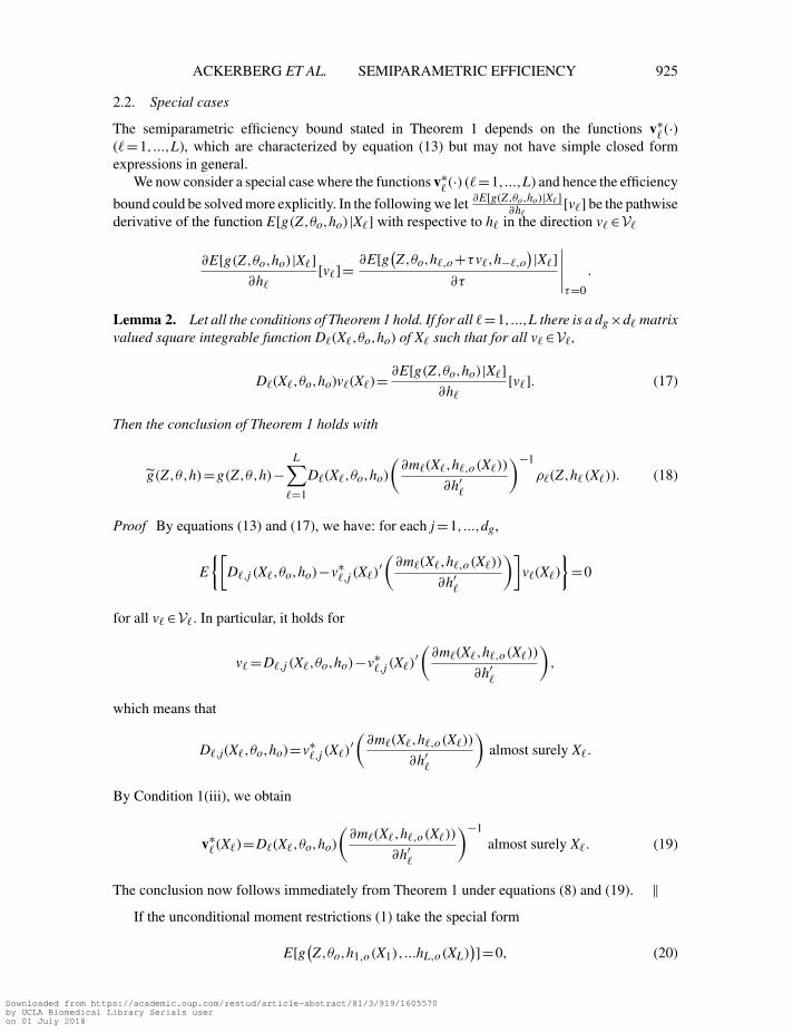
2.2. Special cases

The semiparametric efficiency bound stated in Theorem 1 depends on the functions v∗� (·)

(�=1,...,L), which are characterized by equation (13) but may not have simple closed formexpressions in general.

We now consider a special case where the functions v∗� (·) (�=1,...,L) and hence the efficiency

bound could be solved more explicitly. In the following we let ∂E[g(Z,θo,ho)|X�]∂h�

[v�] be the pathwisederivative of the function E[g(Z,θo,ho)|X�] with respective to h� in the direction v� ∈V�

∂E[g(Z,θo,ho)|X�]∂h�

[v�]=∂E[g(Z,θo,h�,o +τv�,h−�,o

)|X�]∂τ

∣∣∣∣∣τ=0

.

Lemma 2. Let all the conditions of Theorem 1 hold. If for all �=1,...,L there is a dg ×d� matrixvalued square integrable function D�(X�,θo,ho) of X� such that for all v� ∈V�,

D�(X�,θo,ho)v�(X�)= ∂E[g(Z,θo,ho)|X�]∂h�

[v�]. (17)

Then the conclusion of Theorem 1 holds with

g(Z,θ,h)=g(Z,θ,h)−L∑

�=1

D�(X�,θo,ho)

(∂m�(X�,h�,o(X�))

∂h′�

)−1

ρ�(Z,h�(X�)). (18)

Proof By equations (13) and (17), we have: for each j=1,...,dg,

E

{[D�,j (X�,θo,ho)−v∗

�,j (X�)′(

∂m�(X�,h�,o(X�))

∂h′�

)]v�(X�)

}=0

for all v� ∈V�. In particular, it holds for

v� =D�,j (X�,θo,ho)−v∗�,j (X�)

′(

∂m�(X�,h�,o(X�))

∂h′�

),

which means that

D�,j(X�,θo,ho)=v∗�,j (X�)

′(

∂m�(X�,h�,o(X�))

∂h′�

)almost surely X�.

By Condition 1(iii), we obtain

v∗� (X�)=D�(X�,θo,ho)

(∂m�(X�,h�,o(X�))

∂h′�

)−1

almost surely X�. (19)

The conclusion now follows immediately from Theorem 1 under equations (8) and (19). ‖If the unconditional moment restrictions (1) take the special form

E[g(Z,θo,h1,o(X1),...hL,o(XL))]=0, (20)




i.e. if the moment function g depends on ho(·) only through(h1,o(X1),...hL,o(XL)

), then

equation (17) is trivially satisfied with

D�(X�,θo,ho)= ∂E[g(Z,θo,h�,o(X�),h−�,o(X−�

))|X�]∂h′

�

, �=1,...,L,

which could be viewed as an ordinary partial derivative defined similarly as that in equation (4).We next give two examples when the unconditional moment restrictions (1) is of the specialform (20).

Example 1 (Non-parametric Regression) For �=1,...,L, the unknown function h�,o is

identified by the conditional mean restriction: E[

Y�−h�,o(X�)∣∣X�

]=0. Then: ∂m�(X�,h�,o(X�))∂h′

�

=−1 and

g(Z,θ,h)=g(Z,θ,h)+L∑

�=1

∂E[g(Z,θo,ho)|X�]∂h′

�

(Y�−h�(X�)).

Suppose further that (i) L=2, (ii) Z =(Z1,Z2,Z ′3,Z

′4,Z

′5,Z

′6

)such that Z1 and Z2 are scalars, and

(iii) g=(g′1,g

′2

)with

g1(Z,θ,h)=Z5 ×(Z1 −q1(Z3,h1(X1);θ))

g2(Z,θ,h)=Z6 ×(Z2 −q2(Z4,h2(X2);θ))

for some parametrically specified scalar-valued functions q1 and q2. (The models discussed inSection 4 follows a similar structure.) We then have g= (g′

1 ,g′2

)with

g1(Z,θ,h)=Z5 ×(Z1 −q1(Z3,h1(X1);θ))−Z5 × ∂E[q1(Z3,h1,o(X1);θo

)|X1]∂h1

(Y1 −h1(X1))

g2(Z,θ,h)=Z6 ×(Z2 −q2(Z4,h2(X2);θ))−Z6 × ∂E[q2(Z4,h2,o(X2);θo

)|X2]∂h2

(Y2 −h2(X2)).

Example 2 (Non-parametric Quantile Regression) For �=1,...,L, the unknown functionh�,o is identified by the conditional quantile restriction: E

[τ −I{Y� ≤h�,o(X�)}

∣∣X�

]=0.

Denote U� =Y�−h�,o(X�). Let fU� ( ·|X�) be the conditional density of U� given X�. Then:∂m�(X�,h�,o(X�))

∂h′�

=−fU� (0|X�) and

g(Z,θ,h)=g(Z,θ,h)+L∑

�=1

∂E[g(Z,θo,ho)|X�]∂h′

�

(τ −I{Y� ≤h�(X�)})fU� (0|X�)

.

3. DISCUSSION

3.1. Intuition

In order to gain an intuition underlying our result, consider a simple model

E [g(Z;θo,βo)]=0, (21)

where the finite dimensional parameter βo can be identified by

E [ρ(Z;βo)]=0 (22)




We assume that the nuisance parameter βo is exactly identified4 by (22) in the sense that dim(ρ)=dim(β). We also assume that even if βo were known, the finite-dimensional parameter of interestθo is possibly overidentified by (21) in the sense dim(g)≥dim(θ). Note that if the distributionof X has known, finite support, then the semiparametric moment conditions in (1) and (2) can bewritten in (21) and (22).

The information bound for θo can be obtained by the inverse of the upper-left block of(∂E [ϕ(Z;θo,βo)]

∂ (θ ′,β ′)

)′E[ϕ(Z;θo,βo)ϕ(Z;θo,βo)

′]−1(

∂E [ϕ(Z;θo,βo)]

∂ (θ ′,β ′)

),

where we define ϕ by stacking ρ and g vertically, i.e. ϕ′ =(ρ′,g′).Assume further that

∂E [g(Z;θo,βo)]

∂β ′ =0. (23)

Under the regularity condition that ∂E [ρ(Z;βo)]/

∂β ′ is non-singular, it is straightforward toshow that the asymptotic variance bound of θ is equal to the inverse of(

∂E [g(Z;θo,βo)]

∂θ ′)′

E[g(Z;θo,βo)g(Z;θo,βo)

′]−1(

∂E [g(Z;θo,βo)]

∂θ ′)

. (24)

Now, if the assumption (23) is violated, we can consider the following transformation:

g(Z;θ,β)=g(Z;θ,β)−v∗ρ(Z;βo) (25)

such that∂E [g(Z;θo,βo)]

∂β ′ =0 (26)

i.e.

v∗ =(

∂E [g(Z;θo,βo)]

∂β ′)(

∂E [ρ(Z;βo)]

∂β ′)−1

The asymptotic variance of the optimal GMM estimator for the moments

E [g(Z;θo,βo)]=0

E [ρ(Z;βo)]=0

which is obtained by a non-singular transformation of the model (21) and (22), is identical to theoriginal model, but satisfies the zero derivative restriction (26). Therefore, we can conclude thatthe asymptotic variance bound of θ is in general equal to the inverse of(

∂E [g(Z;θo,βo)]

∂θ ′)′

E[g(Z;θo,βo)g(Z;θo,βo)

′]−1(

∂E [g(Z;θo,βo)]

∂θ ′)

=(

∂E [g(Z;θo,βo)]

∂θ

)′E[g(Z;θo,βo)g(Z;θo,βo)

′]−1(

∂E [g(Z;θo,βo)]

∂θ

),

whether the zero derivative restriction (23) is satisfied or not.

4. The discussion in this subsection reflects an anonymous referee’s insight. It also reflects Whitney Newey’sinsight that he kindly shared with us in a private communication.




The v∗ in (25) can also be given the following interpretation. Let β denote a method ofmoments estimator solving the sample counterpart of the exactly identified model (22). Standardarguments can be used to show that

1√n

n∑i=1

g(Zi;θo,β

)= 1√

n

n∑i=1

g(Zi;θo,βo)−(

∂E [g(Z;θo,βo)]

∂β ′)(

∂E [ρ(Z;βo)]

∂β ′)−1 1√

n

n∑i=1

ρ(Zi;βo)+op(1)

= 1√n

n∑i=1

(g(Zi;θo,βo)−v∗ρ(Zi;βo)

)+op(1)

In other words, the v∗ can be understood to be a part of the adjustment of the influence functionof 1√

n

∑ni=1g

(Zi;θo,β

)to reflect the noise of estimating β.

The preceding discussion allows us to provide an alternative interpretation toE[g(Z;θo,βo)g(Z;θo,βo)

′], which is used later in Section 3.3. Suppose that θo is known andthat we define a “parameter” ξo by the moment equation

E [g(Z,θo,βo)−ξo]=0.

A natural estimator of ξo is ξ that sets the sample moment condition 1n

∑ni=1(g(Zi,θo,β

)− ξ)

equal to zero. Note that the asymptotic variance of ξ is equal to that of 1√n

∑ni=1g

(Zi;θo,β

),

which in turn is equal to E[g(Z;θo,βo)g(Z;θo,βo)

′] according to the discussion above.

3.2. Practical implication of Theorem 1

Suppose that ho were known, then we would estimate θo in (1) by Hansen’s (1982) optimallyweighted GMM

minθ∈�

[n−1/2

n∑i=1

g(Zi,θ,ho)

]′W−1

n

[n−1/2

n∑i=1

g(Zi,θ,ho)

]

with Wn =Var [g(Z;θo,ho)]+op(1). Because Var [g(Z;θo,ho)]=Avar(n−1/2∑n

i=1g(Zi,θo,ho)),

the asymptotic variance of such an infeasible GMM estimator would be equal to the inverse of(∂E[g(Z,θo,ho)]

∂θ ′)′(

Avar

(n−1/2

n∑i=1

g(Zi,θo,ho)

))−1(∂E[g(Z,θo,ho)]

∂θ ′)

.

Now ho is in fact unknown, we may consider a feasible version of the preceding GMM estimatorby replacing ho by any consistent non-parametric estimator h and using a weight matrix such thatits probability limit is the inverse of Avar

(n−1/2∑n

i=1g(Zi,θo ,h)); the asymptotic variance of

such a feasible GMM estimator would be the inverse of(∂E[g(Z,θo,ho)]

∂θ ′)′(

Avar

(n−1/2

n∑i=1

g(Zi,θo ,h

)))−1(∂E[g(Z,θo,ho)]

∂θ ′)

. (27)

This feasible GMM estimator was discussed by Newey (1994), Ackerberg et al. (2012), amongothers. Recall our motivation of the paper that it is not obvious (to us at least) whether the feasible




GMM estimator exploits all the information in model (1) and (2), because it does not seem touse, e.g. the (conditional) covariance of the moments between (1) and (2).

A practical implication of our Theorem 1 is that (27) is indeed the semiparametric informationbound for model (1) and (2), and therefore, the feasible GMM estimator discussed above isactually semiparametrically efficient. In order to understand this implication, we need to relateVar (g(Z,θo,ho)) in the middle of (9) in Theorem 1 to the Avar

(n−1/2∑n

i=1g(Zi,θo ,h

))in the

middle of (27):

Proposition 1. For the model (1)–(2), suppose that Condition 1 (i) and (iv) are satisfied. Wethen have

Var (g(Z,θo,ho))=Avar

(n−1/2

n∑i=1

g(Zi,θo ,h

)), (28)

where g is defined in (8) and h is any consistent non-parametric estimator of ho satisfying (2).

Proof We derive the adjustment to the influence function following Newey (1994, pp. 1360–1361). For simplicity, we will assume that L=1 and that h is a scalar, noting that generalizationcan be done in an additive way as discussed in Newey (1994, p. 1357). For a path {Fτ (z)}of the distribution of random variable Z , let hτ to be the function indexed by τ such thatEτ [ρ(Z,hτ (X))|X]=0, where Eτ [ ·|X] denotes the conditional expectation taken under Fτ (z)with the corresponding score S(Z). It follows that

Eτ [w(X)ρ(Z,hτ (X))]=0 (29)

for any square integrable w(X). Differentiating (29) with respect to τ , we obtain

∂

∂τEτ [w(X)ρ(Z,ho(X))]+ ∂

∂τE [w(X)m(X,hτ )]=0. (30)

We can recall the definition of v∗(X), and write

∂

∂τE [g(Z,θo,hτ )]=E

[v∗(X)

(∂

∂τm(X,hτ )

)]= ∂

∂τE[v∗(X)m(X,hτ )

], (31)

which together with (30) implies that

∂

∂τE [g(Z,θo,hτ )]=− ∂

∂τEτ

[v∗(X)ρ(Z,ho(X))

]=Eτ

[−v∗(X)ρ(Z,ho(X))S(Z)]. (32)

It follows that the adjustment term (α in Newey’s notation) is equal to −v∗(X)ρ(Z,ho(X)), andthe influence function of n−1/2∑n

i=1g(Zi,θo ,h

)is equal to

g(Z,θo,ho)−v∗(X)ρ(Z,ho(X))= g(Z,θo,ho).

Next, we note that the Avar(n−1/2∑n

i=1g(Zi,θo ,h

))is invariant to the choice of any consistent

nonparametric estimator h of ho, which follows from Newey’s (1994, Proposition 1) observationthat the asymptotic variance of a semiparametric

√n-consistent estimator is independent of the

types of first step consistent non-parametric estimators. ‖

Remark 1. Note that n−1∑ni=1g

(Zi,θ ,h

)g(Zi,θ ,h

)′usually converges in probability to

Var(g(Z,θo,ho)), which is often different from Avar(n−1/2∑n

i=1g(Zi,θo ,h

)).




3.3. Implementation

The general expression of the information bound of θo in (27) indicates that under suitableregularity conditions, the second step GMM estimator θn that solves

minθ∈�

[n− 1

2

n∑i=1

g(Zi,θ ,h

)]′W−1

n

[n− 1

2

n∑i=1

g(Zi,θ ,h

)], (33)

is semiparametric efficient as long as the weighting matrix Wn satisfies

Wn =Avar

(n−1/2

n∑i=1

g(Zi,θo ,h

))+op(1) (34)

for any consistent non-parametric estimator h of ho.For efficient semiparametric estimation of θo, the crucial step is therefore to consistently

estimate the asymptotic variance of n−1/2∑ni=1g

(Zi,θo ,h

). We describe how this objective

can be achieved using a simple algorithm described in Ackerberg et al. (2012).5 For simplicityof illustration, we assume that for �=1,...,L, the unknown function h�,o is identified by theconditional mean restriction: E

[Y�−h�,o(X�)

∣∣X�

]=0, i.e. we use Example 1.We imagine a researcher, who “pretends” that h�(X�)=p�,1(X�)β(�),1 +···+

p�,K�(X�)β(�),K�

=pK�

� (x�,i)′β(�) =h�

(X�,β(�)

).6 Our researcher equates h with β, and

perceives the latter to be a simple M-estimator solving the moment equation E [ρ(Z;βo)]=0,where

ρ(Z;β)=⎡⎢⎣ pK1

1 (X1)(Y1 −h1

(X1,β(1)

))...

pKLL (XL)

(YL −hL

(XL,β(L)

))⎤⎥⎦. (35)

The researcher then perceives the problem to be a parametric problem characterized by (21) and(22) with ρ(Z;β) defined above in (35).

Using Ackerberg et al. (2012), it can be seen that the following algorithm produces a feasibleestimator of Avar

(n−1/2∑n

i=1g(Zi,θo ,h

)):

1. Estimate β by an M-estimator (e.g. OLS) solving the moment equation E [ρ(Z;βo)]=0,which is equivalent to solving

minβ(�)

n∑i=1

(Y�,i −h�

(X�,i,β(�)

))2�=1,...,L.

2. Using an arbitrary weight matrix, minimize the sample moment 1n

∑ni=1g

(Zi,θ,β

)over

θ to obtain a preliminary estimator θ of θo. Note that our researcher uses a parametricspecification of h, so without loss of generality, we can write g(Z,θ,h)=g(Z,θ,β).

5. Ackerberg et al. (2012) obtain a convenient estimator of standard errors regardless of efficiency issues, but theydo not discuss efficient estimation of θo.

6. The functions p�,1 (X�),p�,2 (X�),... are such that h� (X�) can be well approximated by their linear combination,and K� =K�,n is a function of n to be theoretically correct, although it is perceived to be fixed for our fictitious researcher.




3. Let the “parameter” ξo be defined by the moment

E [g(Z,θo,βo)−ξo]=0.

Pretend that θ =θo and “estimate” ξo with the ξ that sets the sample moment condition1n

∑ni=1(g(Zi,θ,β

)− ξ)

equal to zero. Note that this estimation problem is exactlyidentified. In fact, it is just the mean of the moment conditions evaluated at (θ,β).

4. Again consider θ to be fixed. Note that (β,ξ ) from Steps 1 and 3 can be thought of as anexactly identified “parametric” estimator of (βo,ξo) using the moments

E [ρ(Z;βo)]=0,

E[g(Z,θ,βo

)−ξo]=0.

Use the standard parametric GMM asymptotic variance formula7 to estimate the varianceof (β,ξ ). Denote by Wn the portion of this variance matrix corresponding to ξ . Wn is aconsistent estimator of Avar

(n−1/2∑n

i=1g(Zi,θo ,h

)).

5. Our second-step efficient estimator for θo is simply the solution to

minθ

(1

n

n∑i=1

g(Zi,θ,β

))′W−1

n

(1

n

n∑i=1

g(Zi,θ,β

)).

The components of the above procedure are all very familiar from the parametric GMMliterature, and the procedure is not much harder than a “naive” two-step approach that computesWn by assessing the variance of the second-step moments assuming that (θ,β) are fixed. The“artificial” parameter ξo is just a tool to obtain an estimate of the variance of the second-stepmoments that includes the variance contribution of β (h). In our Monte-Carlo example, wecompare this efficient two-step procedure to both a naive two-step estimator that is not necessarilyefficient and the efficient joint estimator.

Remark 2. Step 4 does require using the standard GMM asymptotic variance formula, which asusual requires computing the derivative of the moments. If analytic derivatives are not possibleor feasible and one prefers not to do numeric differentiation,8 an alternative way to computeAvar

(n−1/2∑n

i=1g(Zi,θo ,h

))in Step 4 is the bootstrap.9 We have to be careful in using the

bootstrap, though. Weak convergence does not imply that the bootstrap variance converges to theasymptotic variance. See Ghosh et al. (1984) or Wu (1986). Hence, if the bootstrap is to be used,a practitioner may want to avoid using the standard bootstrap variance. Alternative methods thathave been shown to produce a consistent estimator of the variance include versions of truncationas suggested in Shao (1992) or Gonçalves and White (2005), and a percentile method as inMachado and Parente (2005).

3.4. Comparison with Chamberlain (1992) and Ai and Chen (2012)

Chamberlain (1992) derived the efficiency bound of θo for the sequential moment restrictions

E[ρt (Y ,X;θo)|X(t)

]=0 with {1}⊆X(0) ⊂X(1) ⊂···⊂X(L)

7. See Newey (1984), Murphy and Topel (1985), Section II of Ackerberg et al. (2012), or standard textbooks suchas Wooldridge (2002, Chapter 12.4). Note that even though (β,ξ ) have been estimated in two steps, the model is exactlyidentified so it is equivalent to joint estimation and thus the standard GMM asymptotic variance formula is used.

8. See, e.g. Hong et al. (2010) for suggestions and caveats regarding numeric differentiation9. See Armstrong et al. (2012), who established the weak convergence of the bootstrap in this case.




for t =0,1,...,L. Ai and Chen (2012) extended the result such that ρt function may depend on anuisance function ho(·). In order to derive the efficiency bound, they proceed by “orthogonalizing”the moments by working with forward filtering as in Hayashi and Sims (1983):

εL (Z,α)=ρL (Z,α),

εs(Z,α)=ρs(Z,α)−L∑

t=s+1

s,t

(X(t)

)εt (Z,α),

where α=(θ,h) and

s,t

(X(t)

)=E

[ρs(Z,αo)εt (Z,αo)

′∣∣X(t)](

�t

(X(t)

))−1,

�t

(X(t)

)=E

[εt (Z,αo)εt (Z,αo)

′∣∣X(t)].

Their efficient estimator is based on forming counterparts of εs(Z,α), which requiresnonparametric estimation of the ’s and �’s.

We can see that our orthogonalization is quite different thanAi and Chen (2012). Theirs is withrespect to covariances of the moments, whereas our orthogonalization is with respect to derivativesof the moments. Perhaps more important from an applied perspective, our orthogonalization isjust a proof technique that can be bypassed in practice by exploiting the algorithm in Section3.3. In contrast, the procedure of Ai and Chen (2012) requires nonparametric implementationof orthogonalization for estimation. As noted in the introduction, our orthogonalization is alsoavailable when the first-step conditioning variables are non-nested. On the other hand, our resultsare limited to the situation where the h is exactly identified, whereas the results in Ai and Chen(2012) do not have such limitation.

4. EXAMPLES AND MONTE CARLO RESULTS

We now illustrate the usefulness of our results and estimators by showing how they can be appliedto two recent methodological literatures that are based on two-step semiparametric techniques.In both examples, our results imply that two-step methods do not need to sacrifice efficiencyrelative to joint estimation. We then do a brief Monte-Carlo study.

4.1. Example 1: Two-Step Estimation of Dynamic Models

Hotz and Miller (1993) initiated a large literature that uses two-step semiparametric estimatorsto estimate single agent dynamic programming problems and dynamic games. The main benefitof the semiparametric approach is to avoid the computational burden associated with solvingdynamic programming problems. With these approaches, one can estimate structural parameterswithout ever having to explicitly solve agents’ dynamic programming problems.

In this literature, two-step estimators are typically preferred to estimators that jointly use allthe moment conditions because of a different computational issue. With a two-step approach,the non-parametric parts of the problem can often be estimated in the first step using analyticestimators (e.g. least squares) or estimators with a globally concave objective function (e.g.logit). This can not only save time but also alleviates concern regarding the reliability of anon-linear search over a large (i.e. asymptotically increasing) set of parameters representing thenon-parametric parts of the problem.




One might worry that such two-step approaches have an efficiency cost, but our resultsshow that this may not be the case. We illustrate this with a simple finite horizon, single agent,dynamic binary choice model. This might be appropriate, e.g. for a model of retirement or fertilitydecisions. One could also apply our results to problems with multiple agents, infinite horizons, andmultinomial choice. However, since our first step relies on estimating conditional expectations,the results do not directly apply to problems with continuous choices (e.g. Bajari et al., 2007).

Suppose that the per-period utility function for agent i making choice yit ∈{0,1} in periodt =1,...,T is given by

U ={

U0(xit;θ )+εi0t if yit =0U1(xit;θ )+εi1t if yit =1

.

The vector xit includes the state variables of the problem (e.g. work experience, number ofchildren, wealth) that are observed by the econometrician. εit ={εi0t,εi1t} represent state variablesthat are not observed by the econometrician. U0 and U1 are known up to the finite dimensionalstructural parameters θ . The majority of the empirical literature thus far has assumed that εit areindependent of xit and i.i.d. over time10, e.g. Type 1 Extreme Value random variables.

Assuming the evolution of the state variable xit is first-order Markov, the optimal policyfunction in this problem is

yit =yt (xit,εit).

The function is indexed by t because of the finite horizon. One can also consider a “conditionalchoice probability”

E [yit |xit]=ht (xit)=∫

yt (xit,εit)p(εit)dεit

which is the probability of making choice 1 in time t given state xit (prior to the agent’s realizationof εit).

The key result of Hotz and Miller (1993) is that under certain conditions, one can rewrite thedynamic programming Bellman equation in terms of conditional choice probabilities, i.e.

ht (xit)=gt(xit,ht+1(·);θ) (36)

where the gt’s are known, (relatively) easily computable, functions.11 This representation ispossible because there is a one-to-one mapping between value functions and conditional choiceprobabilities.

Estimation can then proceed with the following two-step procedure. In the first step, onenon-parametrically estimates the T conditional choice probabilities using

E [yi1 −h1(xi1) | xi1]=0, (37)

.

.

E [yiT −hT (xiT ) | xiT ]=0.

10. see, e.g. Pakes et al. (2007), Pesendorfer and Schmidt-Dengler (2008), Ryan (2012), Collard-Wexler (2012),Fang and Wang (2012). Only recently has the literature considered allowing correlation in unobservables over time, e.g.

Aguirregabiria and Mira (2007), Kasahara and Shimotsu (2009), Hu et al. (2010), and Arcidiacono and Miller (2011),and it is challenging.

11. For the particularly simple form in the text, one needs one of the choices to lead to a terminal state. Hotz et al.(1994) consider finite horizon models without this condition—in that case, all future h’s enter the right hand side. In aninfinite horizon problem, the equation also has a very simple form, since the h function does not depend on time (see,e.g. Aguirregabiria and Mira, 2002)




In the simplest case, the ht functions might be represented by a linear sieve, in which case thefirst step can be performed using simple least squares.12 Note that this set of first stage momentsfalls directly into our framework of non-nested first-step conditioning sets.

In the second step, one can estimate the structural parameters θ using the following momentconditions implied by (36)

E[(

yit −gt(xit ,ht+1(·);θ))⊗r(xit)

]=0 (38)

where the unknown functions ht+1 have been replaced with their estimates from the first step,ht+1. This does not require explicitly solving the agents’dynamic programming problems. Whilethe gt function needs to be computed, this is relatively simple.13

In this context, our results imply that as long as one uses an appropriate weight matrix for thesecond step (e.g. the procedure described in Section 3.3), this two-step procedure does not sacrificeasymptotic efficiency relative to a joint procedure that considers both sets of moments (37) and(38) simultaneously. Again, this is important because the joint procedure requires a non-linearsearch over the entire parameter space (θ,h1,...,hT ), which is likely both more computationallydemanding and less reliable than the two-step approach (which requires a non-linear search overjust θ in the case where linear sieves are used in the first stage14).

4.2. Example 2: two-step estimation of production functions

We next show how our results can be applied to a version of the Olley and Pakes (1996) two-step methodology for estimating production functions. Consider a panel of firms indexed byi producing output yit using inputs xit across time t. The model can be described with threeequations. First is the production function

Production Function: yit =F(xit;θ1)+ωit +εit . (39)

The production function contains two scalar econometric unobservables, ωit and εit . ωit is firmi’s “productivity” shock in period t, and will be permitted to be correlated with input choices xit .In contrast, εit is noise in output (e.g. measurement error) that is assumed to be mean independentof the firm’s information set at t, Iit .

The second equation describes how productivity ωit evolves over time. Specifically, ωit isassumed to follow a first-order Markov process from the firm’s perspective, i.e.

Productivity Evolution: E[ωit |Iit−1

]=μ(ωit−1;θ2). (40)

The last equation describes how some other variable iit is chosen by the firm at t, i.e.

Proxy Choice: iit = i(xit,ωit). (41)

This precise definition of this “proxy” variable iit differs across different formulations of theseestimators. For example, in Olley and Pakes (1996), iit is the firm’s current investment towards

12. Alternatively, one could use a sieve logit or probit.13. See Hotz and Miller (1993) for details. Note that our efficiency result is conditional on a given set

of moments (38), i.e. we do not consider the optimal choice of instrument function r(xit)—for this seePesendorfer and Schmidt-Dengler (2008) in a finite dimensional parameter context.

14. In the case where sieve logits are used in the first stage, the first step would require solving T globally concaveoptimization problems, and the second step would be a non-linear search over θ . Again, this is generally quicker andmore reliable than a non-linear search over the full (θ,h1,...,hT ) space. Moreover, even if the first step does not have aglobal concave objective function, it will generally be easier computationally to estimate the parameters in two steps.




future physical capital. In Levinsohn and Petrin (2003), iit is the firm’s choice of an intermediateinput, e.g. electricity or material input.

In the current formulation, we treat the functions F and μ parametrically, i.e. known up tothe finite dimensional parameters θ1 and θ2. In contrast, the optimal proxy choice function i istreated non-parametrically. This seems somewhat natural since both F and μ can be consideredeconomic primitives of the model, while the i function is not an economic primitive (e.g. in Olleyand Pakes it is the solution to a complicated dynamic investment problem). That said, we shouldnote that this differs slightly from most of the existing empirical literature, which treat both i andμ non-parametrically, and only F parametrically.15

The two key assumptions regarding the Proxy Choice equation are that (i) i(xit,ωit) is strictlymonotonic in ωit , and (ii) ωit is the only econometric unobservable in i(xit,ωit). This implies thattwo firms with the same xit and iit have the same ωit . To make these assumptions more plausible,most empirical researchers using this methodology have allowed the proxy choice equation tovary across t.

iit = it(xit,ωit). (42)

This allows for the general economic environment (e.g. input prices, costs of investment, industrylevel demand, industry structure) firms are operating in to change over time. It also means thattwo firms with the same xit and iit do not necessarily have the same ωit (if they are operating indifferent time periods).16

We also make the assumption that xit ∈ Iit−1 - this is a “timing” assumption that the inputsused in production at time t were decided upon (i.e. committed to) at time t−1.17 This is oftenpartially relaxed in the literature, e.g. in OP and LP, the labour input is not decided until t. Insome case our results can apply to this more general model, but we do not elaborate here to keepthings simple.18

To derive the first-step estimating equation, substitute the inverted (42) into (39), obtaining:

yit =F(xit;θ1)+i−1t (xit,iit)+εit

=ht(xit,iit)+εit .

Note that since xit enters this equation both parametrically (through F), and non-parametrically(through i−1

t ), θ1 and i−1t cannot be separately identified at this stage. Hence, the first step

involves non-parametrically estimating the “composite” functions ht . Common practice in the

15. We need μ to be parametric to fit the model into a two-step procedure in which the second step only requiresestimating a finite dimensional set of parameters. In practice, as long as the parametric μ is specified flexibly, the differenceshould be minor. But strictly speaking, our results only apply when μ is assumed parametric.

16. One can also allow the production function F to depend on t - our results would generalize to this model aswell.

17. This assumption helps provide identification because although xit is correlated with ωit , it implies that xit is notcorrelated with the innovation in ωit , i.e. ωit −E [ωit |Iit−1].

18. Briefly, whether our efficiency result holds depends on whether the structural parameters related to the“variable” inputs can be identified using only the first-step moment condition. If they are, as in the first-step momentof Olley and Pakes (1996), Levinsohn and Petrin (2003), and Wooldridge (2009), our efficiency results does not hold. Ifthey are not, as in the first-step moment of Ackerberg et al. (2006), then our efficiency result does hold.




applied literature is to use the moment conditions

E [εi1 |xi1,ii1 ]=E [yi1 −h1(xi1,ii1)|xi1,ii1 ]=0 (43)

.

.

E [εiT |xiT ,iiT ]=E [yiT −hT (xiT ,iiT )|xiT ,iiT ]=0

and simple kernel or polynomial series regressions of yit on (xit, iit) to estimate each of the ht’sseparately. Thus, this again falls into our framework of non-nested conditioning sets.

For the second step estimating equation, take the conditional expectation of (39) given Iit−1,substitute in (40), and then substitute in the inverted (42), i.e.

E[yit |Iit−1

] =E[F(xit;θ1)+ωit +εit |Iit−1

]=F(xit;θ1)+E

[ωit |Iit−1

]+0

=F(xit;θ1)+μ(ωit−1;θ2)

=F(xit;θ1)+μ(i−1t−1(xit−1,iit−1);θ2)

=F(xit;θ1)+μ(ht−1(xit−1,iit−1)−F(xit−1;θ1);θ2).

The finite dimensional parameters θ1 and θ2 are then estimated using the moment condition:

E[(

yit −F(xit;θ1)−μ(ht−1(xit−1,iit−1)−F(xit−1;θ1);θ2))⊗r(Iit−1)

]=0 (44)

where the unknown functions ht have been replaced with their estimates from the first step, ht .Note that since we started by assuming E [εit |Iit]=0 (and Iit includes past i’s and x’s), the first

step moments (43) likely do not exhaust all the information in the model. But our results showthat if, as typically done in practice, one only uses this limited set of first-step moments19, thetwo-step procedure (with appropriate second-step weight matrix) does not sacrifice asymptoticefficiency relative to a joint procedure. Again, this is important because the joint procedure wouldrequires non-linear optimization over both θ and the ht’s simultaneously, which is considerablymore computationally burdensome (and prone to error) than the two-step approach, which inmost cases only requires non-linear optimization over θ .

4.3. Small Monte Carlo experiment

We perform a brief Monte-Carlo experiment in the context of the above production functionexample to examine the performance of the various estimators in a small sample context. Weconsider the following Cobb–Douglas production function in logs

yit =θ0 +θ1kit +ωit +εit

where θ0 =0 and θ1 =1. Firms accumulate capital according to (note that uppercase variables arenot logged)

Kit =δKit−1 +κit Iit−1

19. Presumably applied researchers do this because of the ease of running simple kernel or series regressions. Itwould be more complicated to enforce all the moment conditions (i.e. w.r.t. the full Iit) to estimate the ht functions.




TABLE 1Monte Carlo results

Naive Efficient two-step Joint

Truth Mean S.D. Mean S.D. Mean S.D.

Exact polynomial approximation (1000 reps)θ0 0 −0.0010 0.0522 −0.0009 0.0484 −0.0006 0.0484θ1 1 1.0002 0.0202 1.0004 0.0186 1.0002 0.0187θ2 0.7 0.6972 0.0361 0.6974 0.0314 0.6999 0.0316

Non-exact polynomial approximation (1000 reps)θ0 0 0.0143 0.0659 −0.0216 0.0565 −0.0146 0.0563θ1 1 0.9930 0.0259 1.0089 0.0222 1.0058 0.0220θ2 0.7 0.7245 0.0433 0.7098 0.0344 0.7243 0.0351

where δ=0.9 and κit is a lognormal shock to the capital accumulation process. Firms investmentdecisions are assumed to follow

iit =γ0 +γ1kit +γ2ωit (45)

where γ0 =0, γ1 =−0.1, and γ2 =1. This investment process is admittedly ad hoc but veryconvenient since it (i) allows us to do the Monte-Carlos without having to solve firms’ dynamicprogramming problems, and (ii) allows us to run a specification where the non-parametricapproximation is exact. We consider 1000 firms, and assume we observe two periods of fulldata for each firm (plus a lag - period 0). We do a 1000 period run-in prior to the observed data,so the data can be thought of as coming from the steady-state distribution given the specifiedinvestment process.

The productivity shock ωit is assumed to follow a normal AR(1) process with depreciationparameter θ2 =0.7. The variance of the innovation term in the AR(1) is set such that σω =0.1.The measurement error in output, εit is normal and i.i.d. over i and t. We vary σε across the threerelevant periods in the data - σε0 =0.2, σε1 =0.05 and σε2 =0.1. This is important because inour simple model, this heterogeneity in σε generates an efficiency advantage of joint estimationrelative to naive two-step estimation. Intuitively, the heterogeneity in σε means that the differenth’s are estimated with different precision, which is accounted for in joint estimation (and ourprocedure), but not in the “naive” two-step approach. The lognormal capital accumulation shockκit is assumed to be i.i.d. over i and t and where the variance of the underlying normal is 1.20

Following the discussion in the prior subsection, we use iit as the “proxy” variable. This leadsto the first-step moment conditions

E [εi0 |ki0,ii0 ]=E [yi0 −h0(ki0,ii0)|ki0,ii0 ]=0, (46)

E [εi1 |ki1,ii1 ]=E [yi1 −h1(ki1,ii1)|ki1,ii1 ]=0.

We model h0 and h1 as second-order polynomials in the two arguments. Because (45) is linear, thenon-parametric approximation is exact in this case (and while we still estimate the second-orderterms, they are irrelevant). We also consider a case where we replace kit and iit with Kit and Iit

20. The relatively low variance of ω and ε and relatively high variance of κ (which generates more variation inobserved kit) helps lower the variance of all the estimators. Relatedly, it also makes the objective function more concave,which helps the reliability of the numeric optimization algorithm. This is particularly important to have confidence in theresults of joint estimation procedure because that requires a non-linear search over 15 parameters.




(non-logged variables) in (46) and assume the h’s are linear. Since ωit is not linear in Kit and Iit ,in this case the polynomial approximation is not exact. The second-step moment conditions are

E[(

yi1 −θ0 −θ1ki1 −θ2(h0(ki0,ii0)−θ0 −θ1ki0))⊗[1,ki0,ki1,ii0]

]=0, (47)

E[(

yi2 −θ0 −θ1ki2 −θ2(h1(ki1,ii1)−θ0 −θ1ki1))⊗[1,ki1,ki2,ii1]

]=0.

Results are in Table 1. We estimate the model three ways—efficient joint estimation of bothsets of moments (“Joint”), our proposed two-step efficient estimator from Section 3.3 (“EfficientTwo-Step”), and a naive two-step estimator that does not consider the effect of h in constructing thesecond-step weight matrix (“Naive”).21 Confirming our theoretical results, the efficient two-stepestimator performs almost identically to the joint estimator, and both have a smaller small samplevariance than the naive two-step estimator. This is true regardless of whether the polynomialapproximation subsumes the true specification.

5. SUMMARY

This article studies the efficiency issue of a general two-step GMM estimation procedure, wherethe “exactly identified” unknown nuisance functions are estimated first and the finite dimensionalparameters of interest are estimated by GMM with the first-step non-parametric estimators. Wecalculate the semiparametric efficiency bound for these models, and show that semiparametrictwo-step optimally weighted GMM estimators achieve the efficiency bound, where the nuisancefunctions could be estimated via any consistent nonparametric methods in the first step. Regardlessof whether the efficiency bound has a closed form expression or not, we provide easy-to-compute sieve based optimal weight matrices that lead to asymptotically efficient two-step GMMestimators.

It is not yet clear whether or how the results would generalize to the case where the first-step non-parametric estimator takes the form of a non-parametric instrumental variables (NPIV)estimator. This is an important challenge that we leave as a future research agenda.

APPENDIX

A. PROOF OF THE MAIN RESULTS IN SECTION 2

Let Fo(·) be the unknown true probability distribution of Z . For �=1,...,L with a fixed finite L, let F�,o(·|x�) be theunknown true conditional probability distribution of Z−� given X� =x�, where Z−� denotes the components of Z not inthe conditioning variable X�, and hence Z = (Z ′−�,X

′�)′. The model (1)–(2) can be rewritten∫

g(z,θo,h1,o(·),...,hL,o(·))dFo(z)=0, (A.1)∫

ρ�

(z−�,x�,h�,o(x�)

)dF�,o(z−�|x�)=0 for almost all x�, �=1,...,L. (A.2)

We note that although the unknown functions h�,o(·), �=1,...,L enter the conditional moment restrictions (2) (i.e. (A.2))through h�,o(X�) only, they could enter the unconditional moment restrictions (1) (i.e. (A.1)) in a very flexible way.We assume that the infinite dimensional nuisance functions ho(·)= (h1,o(·),...,hL,o(·))∈H=H1 ×···×HL are identifiedby the conditional moment restrictions (A.2), and that if ho(·) were known, the finite dimensional parameter θo ∈� is(possibly) over identified by the unconditional moment restrictions (A.1).

21. In all three cases, we need an initial consistent estimate of (θ,h) to form weight matrices. For all three cases,we use a h from the first-step polynomial OLS regression, and a θ obtained by minimizing the second-step momentswith a weight matrix given by Var([ξ0i,ξ0iki0,ξ0iki1,ξ0i ii0,ξ1i,ξ1iki1,ξ1iki2,ξ1i ii1])−1 where ξ0i and ξ1i are i.i.d. standardnormals.




Proof of Lemma 1. For the ease of notation and without loss of generality, we assume in this proof that L=2. We assumethat the regularity condition as in Newey (1990), Definition A.1) is satisfied.

Let fo(z) to be the true density of Z with respect to a sigma finite dominating measure μ(z), and fo(z−�|x�) be the trueconditional density of Z−� given X� =x� (�=1,2). Here F denotes a class of candidate density function of Z with fo ∈F .Define a class of density functions Fα that satisfy the conditional and unconditional moment conditions:

Fα ={

f ∈F :∫

ρ1 (z−1,h1(x1))f (z−1|x1)dμ(z−1)=0,∫ρ2 (z−2,h2(x2))f (z−2|x2)dμ(z−2)=0,∫

g(z,θ,h1,h2)f (z)dμ(z)=0

}. (A.3)

We will consider a class of densities of Z indexed by (θ,h1,h2,η), where η denotes the parameter that determines thefeatures of the distribution of Z other than the restriction above. More precisely, let G denote a class of real-valuedmeasurable function of Z such that

Fα ={ f ( z|θ,h1,h2,η) :η∈G} (A.4)

for any α= (θ,h1,h2)∈�×H1 ×H2. Let Vθ ×V1 ×V2 ×Vη denote the completion (with respect to the L2-norm) of�×H1 ×H2 ×G−{(θo,h1,o,h2,o,ηo)} where ηo satisfies

f(

z|θo,h1,o,h2,o,ηo)= fo(z).

We will consider the parametric family f(

z|θo +θ,h1,o +τ1v1,h2,o +τ2v2,ηo +τηvη

)in Fα . The scores in the direction

of θ , τ1, τ2, τη of this family are such that

sθ (Z)=cθ,1 ( Z−1|X1)+dθ,1 (X1)

=cθ,2 ( Z−2|X2)+dθ,2 (X2),

sh1 (Z)[v1]=ch1,1 ( Z−1|X1)[v1]+dh1,1 (X1)[v1]

=ch1,2 ( Z−2|X2)[v1]+dh1,2 (X2)[v1],

sh2 (Z)[v2]=ch2,1 ( Z−1|X1)[v2]+dh2,1 (X1)[v2]

=ch2,2 ( Z−2|X2)[v2]+dh2,2 (X2)[v2],

sη (Z)[vη

]=cη,1 ( Z−1|X1)[vη

]+dη,1 (X1)[vη

]=cη,2 ( Z−2|X2)

[vη

]+dη,2 (X2)[vη

],

with

E[

cθ,1 (Z−1,X1)∣∣X1

]=0, (A.5)

E[dθ,1 (X1)

]=0, (A.6)

E[

cθ,2 (Z−2,X2)∣∣X2

]=0, (A.7)

E[dθ,2 (X2)

]=0, (A.8)

E[

ch1,1 ( Z−1|X1)[v1]∣∣X1

]=0, (A.9)

E[dh1,1 (X1)[v1]

]=0, (A.10)

E[

ch2,1 ( Z−1|X1)[v1]∣∣X1

]=0, (A.11)

E[dh2,1 (X1)[v1]

]=0, (A.12)

E[

ch2,2 ( Z−2|X2)[v2]∣∣X2

]=0, (A.13)

E[dh2,2 (X2)[v2]

]=0, (A.14)

E[

ch1,2 ( Z−2|X2)[v2]∣∣X2

]=0, (A.15)

E[dh1,2 (X2)[v2]

]=0, (A.16)




and

E[

cη,1 (Z−1,X1)[vη

]∣∣X1]=0, (A.17)

E[dη,1 (X1)

[vη

]]=0, (A.18)

E[

cη,2 (Z−2,X2)[vη

]∣∣X2]=0, (A.19)

E[dη,2 (X2)

[vη

]]=0. (A.20)

Here, ch1 ( Z−1|X1)[v1] and dh1 (X1)[v1] denote the conditional score of Z−1 given X1 and the marginal score of X1,obtained by differentiating the log-likelihood with respect to τ1, for example. Note that sθ (Z) is a dθ ×1 vector offunctions. Below, we will write ch1 (Z)[v1]≡ch1 ( Z−1|X1)[v1], e.g. for simplicity of notations.

Differentiating the moment restrictions in (A.3), we obtain the non-parametric tangent space T as the completion ofthe set consisting of sh1 (Z)[v1]+sh2 (Z)[v2]+sη (Z)

[vη

], where s’s satisfy (A.5)–(A.20) as well as

E[ρ1(Z,h1,o

)cθ,1 (Z)′

∣∣X1]=0, (A.21)

∂m1(X1,h1,o (X1))

∂h′1

v1 (X1)+E[ρ1(Z,h1,o

)ch1,1 (Z)[v1]

∣∣X1]=0, (A.22)

E[ρ1(Z,h1,o

)ch2,1 (Z)[v2]

∣∣X1]=0, (A.23)

E[ρ1(Z,h1,o)cη,1 (Z)

[vη

]∣∣X1]=0, (A.24)

E[ρ2(Z,h2,o)cθ,2 (Z)′

∣∣X2]=0, (A.25)

E[ρ2(Z,h2,o)ch1,2 (Z)[v1]

∣∣X2]=0, (A.26)

∂m2(X2,h2,o (X2))

∂h′2

v2 (X2)+E[ρ2(Z,h2,o)ch2,2 (Z)[v2]

∣∣X2]=0, (A.27)

E[ρ2(Z,h2,o)cη,2 (Z)

[vη

]∣∣X2]=0, (A.28)

and

∂E[g(Z,θo,h1,o,h2,o

)]∂θ ′ +E

[g(Z,θo,h1,o,h2,o

)sθ (Z)′

]=0, (A.29)

E[g(Z,θo,h1,o,h2,o)sh1 (Z)[v1]]=0, (A.30)

E[g(Z,θo,h1,o,h2,o

)sh2 (Z)[v2]

]=0, (A.31)

E[g(Z,θo,h1,o,h2,o

)sη (Z)

[vη

]]=0, (A.32)

for any (v1,v2,vη)∈V1 ×V2 ×Vη , where ∂m�(X�,h�,o(X�))∂h′

�

and v� (X�) are d� ×d� matrix of functions and d� ×1 vector of

functions respectively. Note that (14) is used in (A.30) and (A.31).The residual of the projection of sθ on T , sθ (Z)−proj[ sθ (Z)|T ] will give the semiparametric score S∗

θ (Z) and thesemiparametric information bound of θo will be E[S∗

θ (Z)S∗θ (Z)′]. See Bickel et al. (1993) and Newey (1990). We show

that the residual of the projection of sθ on T is equal to

S∗θ (Z)=−

(∂E[g(Z)]

∂θ ′

)′{E[g(Z)g(Z)′

]}−1g(Z) (A.33)

where g(Z)=g(Z,θo,h1,o,h2,o

).

We now define �∗1 (X1) and �∗

2 (X2) as solutions to

0=E[ρ1(Z,h1,o)

{cθ,1 (Z)′ −S∗

θ (Z)′ −ch1,1 (Z)[�∗

1

]−ch2,1 (Z)[�∗

2

]}∣∣X1]

(A.34)

and0=E

[ρ2(Z,h2,o)

{cθ,2 (Z)′ −S∗

θ (Z)′ −ch1,2 (Z)[�∗

1

]−ch2,2 (Z)[�∗

2

]}∣∣X2]. (A.35)

Note that for �=1,2, �∗� (X�) is a d� ×dθ matrix of functions and

ch�,� (Z)[�∗

�

]=[ch�,� (Z)[�∗

�,1

],...,ch�,� (Z)

[�∗

�,dθ

]]is a 1×dθ vector of functions, where �∗

�,j (X�) denotes the j-th row of �∗� (X�) for j=1,...,dθ .




We argue that such �∗1 (X1) and �∗

2 (X2) exist as unique objects almost surely for the following reason. Lettingv1 =�∗

1,j (X1) in (A.22) and v2 =�∗2,j (X2) in (A.23) for j=1,...,dθ , we get

∂m1(X1,h1,o (X1))

∂h′1

�∗1 (X1)+E

[ρ1(Z,h1,o

)ch1,1 (Z)

[�∗

1

]∣∣X1]=0 (A.36)

andE[ρ1(Z,h1,o

)ch2,1 (Z)

[�∗

2

]∣∣X1]=0. (A.37)

Using (A.21), (A.33), (A.36), and (A.37), we note that

E[ρ1(Z,h1,o)cθ,1 (Z)′

∣∣X1]−E

[ρ1(Z,h1,o)S∗

θ (Z)′∣∣X1

]−E

[ρ1(Z,h1,o)ch1,1 (Z)

[�∗

1

]∣∣X1]−E

[ρ1(Z,h1,o)ch2,1 (Z)

[�∗

2

]∣∣X1]

=0+(

∂E[g(Z)]∂θ ′

)′{E[g(Z)g(Z)′

]}−1E[

g(Z)ρ1(Z,h1,o)′∣∣X1

]+(

∂m1(X1,h1,o (X1))

∂h′1

�∗1 (X1)

)′+0,

so we rewrite (A.34) as

0=E[ρ1(Z,h1,o

)g(Z)′

∣∣X1]{

E[g(Z)g(Z)′

]}−1 ∂E[g(Z)]∂θ ′ + ∂m1(X1,h1,o (X1))

∂h′1

�∗1 (X1),

which can be solved for �∗1 (X1) as long as ∂m1

(X1,h1,o (X1)

)/∂h′

1 is invertible almost surely. Similarly, we can solvefor �∗

2 (X2) as long as ∂m2(X2,h2,o (X2)

)/∂h′

2 is invertible almost surely.Now let

δ′ =sθ (Z)′ −S∗θ (Z)′ −sh1 (Z)

[�∗

1

]−sh2 (Z)[�∗

2

].

We will show that δ satisfies the properties (A.17)–(A.20), (A.24), (A.28), and (A.32) of the sη (Z)[vη

]for some vη .

• By construction, we have E [δ]=0. Taking

dη,1 (X1)[vη

]=E [ δ|X1]

=dθ,1 (X1)−(dh1,1 (X1)

[�∗

1

])′ −(dh2,1 (X1)[�∗

2

])′+E

[cθ,1 (Z)−S∗

θ (Z)−(ch1,1 (Z)[�∗

1

])′ −(ch2,1 (Z)[�∗

2

])′∣∣∣X1

]=dθ,1 (X1)−

(dh1,1 (X1)

[�∗

1

])′ −(dh2,1 (X1)[�∗

2

])′ −E[

S∗θ (Z)

∣∣X1],

and

cη,1 (Z)[vη

]=δ− dη,1 (X1)[vη

]=cθ,1 (X1)−

(ch1,1 (Z)

[�∗

1

])′ −(ch2,1 (Z)[�∗

2

])′ −S∗θ (Z)+E

[S∗

θ (Z)∣∣X1

],

we can see that properties (A.17) and (A.18) are satisfied for

δ= cη,1 (Z)[vη

]+ dη,1 (X1)[vη

].

With cη,2 (Z)[vη

]and dη,2 (X2)

[vη

]similarly defined, we can see that properties (A.19) and (A.20) are also satisfied.

• Equations (A.34) implies that

E[ρ1(Z,h1,o )cη,1 (z)

[vη

]′∣∣∣X1

]=E

[ρ1(Z,h1,o)

{cθ,1 (Z)′ −S∗

θ (Z)′ −ch1,1 (Z)[�∗

1

]−ch2,1 (Z)[�∗

2

]}∣∣X1]

+E[ρ1(Z,h1,o)

∣∣X1]E[

S∗θ (Z)′

∣∣X1]

=0.

which implies that the property (A.24) is satisfied by δ. Likewise, (A.28) are satisfied by δ.




• Using (A.29)–(A.31), we obtain

E[δg(Z)′

]=E[sθ (Z)g(Z)′

]−E[S∗

θ (Z)g(Z)′]

=−(

∂E[g(Z)]∂θ ′

)′+(

∂E[g(Z)]∂θ ′

)′{E[g(Z)g(Z)′]}−1{

E[g(Z)g(Z)′]}=0, (A.38)

which shows that the property (A.32) is satisfied.

These observations lead us to conclude that

sh1 (Z)[�∗

1

]+sh2 (Z)[�∗

2

]+δ∈T . (A.39)

Because S∗θ (Z) is proportional to g(Z), we can deduce from (A.30) to (A.32) that S∗

θ (Z)⊥T . Along with (A.39), thisimplies that S∗

θ (Z) is the residual of the projection of sθ on T . Thus the semiparametric information bound of θo is

E[S∗θ (Z)S∗

θ (Z)′]=(

∂E[g(Z)]∂θ ′

)′{E[g(Z)g(Z)′]}−1

(∂E[g(Z)]

∂θ ′

). (A.40)

‖

Acknowledgments. We acknowledge helpful comments from R. Blundell, T. Christensen, A. Gandhi, W. Newey,A. Pakes, D. Pouzo, J. Powell, E. Renault and participants in May 2012 Cemmap Masterclass on Semi-nonparametricModels and Methods in London, inAugust 2012 NBER-NSF CEME Conference on The Econometrics of Dynamic Gamesat NYU, in November 2012 Info-metrics & Nonparametric Inference at UC Riverside and econometrics workshops atBoston University, UC-Berkeley, UC-Davis, USC and University of Washington. Any errors are the responsibility of theauthors.

Supplementary Data

Replication files for the simulations of Section 4.3 are included in Supplementary data, which are available at Review ofEconomic Studies online.

REFERENCES

ACKERBERG, D., CAVES, K. and FRAZER, G. (2006), “Structural Identification of Production Functions” (mimeo,UCLA).

ACKERBERG, D., CHEN, X. and HAHN, J. (2012), “A Practical Asymptotic Variance Estimator for Two-StepSemiparametric Estimators”, Review of Economics and Statistics, 94, 481–498.

AGUIRREGABIRIA, V. and MIRA, P. (2002), “Swapping the Nested Fixed Point Algorithm: A Class of Estimators forDiscrete Markov Decision Models”, Econometrica, 70, 1519–1543.

AGUIRREGABIRIA, V., and MIRA, P. (2007), “Sequential Estimation of Dynamic Discrete Games”, Econometrica, 75,1–53.

AI, C. and CHEN, X. (2003), “Efficient Estimation of Conditional Moment Restrictions Models Containing UnknownFunctions”, Econometrica, 71, 1795–1843.

AI, C. and CHEN, X. (2007), “Estimation of Possibly Misspecified Semiparametric Conditional Moment RestrictionModels with Different Conditioning Variables”, Journal of Econometrics, 141, 5–43.

AI, C. and CHEN, X. (2012), “The Semiparametric Efficiency Bound for Models of Sequential Moment RestrictionsContaining Unknown Functions”, Journal of Econometrics, 170, 442–457.

ANDREWS, D. (1994), “Asymptotics for Semi-parametric Econometric Models via Stochastic Equicontinuity”,Econometrica, 62, 43–72.

ARCIDIACONO, P. and MILLER, R. (2011), “Conditional Choice Probability Estimation of Dynamic Discrete ChoiceModels with Unobserved Heterogeneity”, Econometrica, 79, 1823–1868.

ARMSTRONG, T. B., BERTANHA, M. and HONG, H. (2012), “A Fast Resample Method for Parametric andSemiparametric Models” (Unpublished working paper).

BAJARI, P., BENKARD, L. and LEVIN, J. (2007), “Estimating Dynamic Models of Imperfect Competition”,Econometrica, 75, 1331–1370.

BICKEL, P. J., KLAASSEN, C. A. J., RITOV, Y. and WELLNER, J. A. (1993), Efficient and Adaptive Inference inSemiparametric Models (Baltimore: Johns Hopkins University Press).

CHAMBERLAIN, G. (1992), “Comment: Sequential Moment Restrictions in Panel Data”, Journal of Business andEconomic Statistics, 10, 20–26.

CHEN, X., LINTON, O. and VAN KEILEGOM, I. (2003), “Estimation of Semiparametric Models when the CriterionFunction is not Smooth”, Econometrica, 71, 1591–1608.


http://restud.oxfordjournals.org/lookup/suppl/doi:10.1093/restud/rdu011/-/DC1



COLLARD-WEXLER, A. (2012), “Demand Fluctuations in the Ready-Mix Concrete Industry” Econometrica(forthcoming).

CREPON, B., KRAMARZ, F. and TROGNON, A. (1997), “Parameters of Interest, Nuisance Parameters, andOrthogonality Conditions: An Application to Autoregressive Error Component Models”, Journal of Econometrics, 82,135–156.

FANG, H. and WANG, Y. (2012), “Estimating Dynamic Discrete Choice Models with Hyperbolic Discounting with anApplication to Mammorgraphy Decisions” (Working paper, University of Pennsylvania).

GHOSH, M., PARR, W.C. and SINGH, K. (1984), “A Note on Bootstrapping the Sample Median”, Annals of Statistics,12, 1130–1135.

GONÇALVES, S. and WHITE, H. (2005), “Bootstrap Standard Error Estimates for Linear Regression”, Journal ofAmerican Statistical Association, 100, 970–979.

HAYASHI, F. and SIMS, C. (1983), “Nearly Efficient Estimation of Time Series Models with Predetermined, but notExogenous Instruments”, Econometrica, 51, 783–798.

HONG, H., MAHAJAN, A. and NEKIPELOV, D. (2010), “Extremum Estimation and Numerical Derivatives” (mimeo,Stanford University).

HOTZ, J. and MILLER, R. (1993), “Conditional Choice Probabilities and the Estimation of Dynamic Models”, Reviewof Economic Studies, 60, 497–529.

HOTZ, J., MILLER, R., SANDERS, S. and SMITH, J. (1994), “A Simulation Estimator for Dynamic Models of DiscreteChoice”, Review of Economic Studies, 61, 265–289.

Hu, Y., Shum, M., and Tan, W. (2010), “ASimple Estimator for Dynamic Models with Serially Correlated Unobservables”(Unpublished working paper).

HANSEN, L. P. (1982), “Large Sample Properties of Generalized Method of Moments Estimators”, Econometrica, 50,1029–1054.

KASAHARA, H. and SHIMOTSU, K. (2009), “Nonparametric Identification and Estimation of Finite Mixture Modelsof Dynamic Discrete Choices”, Econometrica, 77, 135–175.

LEVINSOHN, J. and PETRIN, A. (2003), “Estimating Production Functions using Inputs to Control for Unobservables”,Review of Economic Studies, 70, 317–341.

MACHADO, J.A. F., and PARENTE, P. (2005), “Bootstrap Estimation of Covariance Matrices via the Percentile Method”,Econometrics Journal, 8, 70–78.

MURPHY, K. M. and TOPEL, R. H. (1985), “Estimation and Inference in Two-Step Econometric Models”, Journal ofBusiness and Economic Statistics, 3, 370–379.

NEWEY, W. K. (1984), “AMethod of Moments Interpretation of Sequential Estimators”, Economics Letters, 14, 201–206.NEWEY, W. K. (1990), “Semiparametric Efficiency Bounds”, Journal of Applied Econometrics, 5, 99–135.NEWEY, W. K. (1994), “The Asymptotic Variance of Semiparametric Estimators”, Econometrica, 62, 1349–1382.NEWEY, W. K. and POWELL, J. L. (1999), “Two-step Estimation, Optimal Moment Conditions, and Sample Selection

Models” (Working paper, MIT).OLLEY, G. and PAKES, A. (1996), “The Dynamics of Productivity in the Telecommunications Equipment Industry”,

Econometrica, 64, 1263–1297.PAKES, A. and OLLEY, G. (1995), “A Limit Theorem for a Smooth Class of Semiparametric Estimators”, Journal of

Econometrics, 65, 295–332.PAKES, A., OSTROVSKY, M. and BERRY, S. (2007), “Simple Estimators for the Parameters of Discrete Dynamic

Games, with Entry/Exit Examples”, RAND Journal of Economics, 38, 373–399.PESENDORFER, M. and SCHMIDT-DENGLER, P. (2008), “Asymptotic Least Squares Estimators for Dynamic Games”,

Review of Economic Studies, 75, 901–928.RYAN, S. (2012), “The Costs of Environmental Regulation in a Concentrated Industry”, Econometrica, 80, 1019–1061.SHAO, J. (1992), “Bootstrap Variance Estimators with Truncation”, Statistics & Probability Letters, 15, 95–101.WOOLDRIDGE, J. M. (2002), Econometric Analysis of Cross Section and Panel Data (Cambridge: MIT Press).WOOLDRIDGE, J. M. (2009), “On Estimating Firm-Level Production Functions Using Proxy Variables to Control

for.Unobservables”, Economics Letters, 104, 112–114.WU, C. F. J. (1986), “Jackknife, Bootstrap and Other Resampling Methods in Regression Analysis”, Annals of Statistics,

14, 1261–1295.


Documents

Asymptotic Efﬁciency of Semiparametric Two-step GMM