Asymptotic Expansion Method for SingularPerturbation Problem

Thesis submitted in partial fulfillment of the requirements

for the degree of

Master of Science

by

Gayatri Satapathy

Under the guidance of

Prof. Jugal Mohapatra

Department of MathematicsNational Institute of Technology

Rourkela-769008

India

June, 2012

ii

Declaration

I hereby certify that the work which is being presented in the thesis entitled “Asymptotic

Expansion Method for Singular Perturbation Problem” in partial fulfillment of the re-

quirement for the award of the degree of Master of Science, submitted in the Department

of Mathematics, National Institute of Technology, Rourkela is a review work carried out

under the supervision of Dr. Jugal Mohapatra. The matter embodied in this thesis has

not been submitted by me for the award of any other degree.

(Gayatri Satapathy)

Roll No-410MA2107

This is to certify that the above statement made by the candidate is true to the best of

my knowledge.

Dr. Jugal MohapatraAssistant Professor

Place: NIT Rourkela Department of MathematicsDate: June 2012 NIT Rourkela-769008

India

iv

Acknowledgement

It is of great pleasure and proud privilege to express my deep sense of gratitude to my

supervisor Prof. Jugal Mohapatra. I am grateful for his indispensable encouragement

and guidance throughout the period of my project work. Without his active guidance, it

would have not been possible to complete the work.

I acknowledge my sincere gratitude to the Head, all faculty members, all non-teaching

staffs of the Department of Mathematics and the authorities of NIT Rourkela.

I also, thank to all my friends for their kind support, co-operation and help in various ways

during my tenure at NIT Rourkela. I express my sincere thank with gratitude to my par-

ents and other family members for their extended support, blessings and encouragement.

Finally, I bow down before the almighty who has made everything possible.

Place: NIT Rourkela

Date: June 2012 (Gayatri Satapathy)

Roll No-410MA2107

vi

Abstract

The main purpose of this thesis is to address the application of perturbation expansion

techniques for the solution perturbed problems, precisely differential equations. When

a large or small parameter ‘ε’ known as the perturbation parameter occurs in a mathe-

matical model, then the model problem is known as a perturbed problem. Asymptotic

expansion technique is a method to get the approximate solution using asymptotic series

for model perturbed problems. The asymptotic series may not and often do not converge

but in a truncated form of only two or three terms, provide a useful approximation to the

original problem. Though the perturbed differential equations can be solved numerically

by using various numerical schemes, but the asymptotic techniques provide an awareness

of the solution before one compute the numerical solution. Here, perturbation expansion

for some model algebraic and differential equations are considered and the results are

compared with the exact solution.

viii

Contents

1 Motivation 1

1.1 Introduction . . . . . . . . . . . . . . . . . . . . . . . . . . . . . . . . . . . 1

1.2 Mathematical model . . . . . . . . . . . . . . . . . . . . . . . . . . . . . . 2

1.3 Asymptotic expansion . . . . . . . . . . . . . . . . . . . . . . . . . . . . . 4

1.3.1 Order symbols . . . . . . . . . . . . . . . . . . . . . . . . . . . . . . 5

1.3.2 Asymptotic expansion . . . . . . . . . . . . . . . . . . . . . . . . . 5

2 Perturbation Techniques 7

2.1 Regularly perturbed problem . . . . . . . . . . . . . . . . . . . . . . . . . 7

2.2 Singularly perturbed problem . . . . . . . . . . . . . . . . . . . . . . . . . 10

2.3 Matched asymptotic expansion . . . . . . . . . . . . . . . . . . . . . . . . 13

3 Conclusion and Future work 17

3.1 Conclusion . . . . . . . . . . . . . . . . . . . . . . . . . . . . . . . . . . . . 17

3.2 Future work . . . . . . . . . . . . . . . . . . . . . . . . . . . . . . . . . . . 18

Bibliography 19

1

2

Chapter 1

Motivation

1.1 Introduction

The study of perturbation problem is important as they arises in several branches of engi-

neering and applied mathematics. The word “ perturbation” means a small disturbance

in a physical system. Mathematically, “perturbation method” is a method for obtain-

ing approximate solution to complex equations (algebraic or differential) for which exact

solution is not easy to find. Mainly, such problems which contain at least one small pa-

rameter ε known as perturbation parameter. We generally denote ε for the effect of small

disturbance in physical system and ε is significantly less than unity.

Mathematicians and engineers study the behavior of the analytical solution of per-

turbed problems through asymptotic expansion technique which combines a straightfor-

ward perturbation expansion using an asymptotic series in the small parameter ε as ε

goes to zero. Below, we have discussed the outline of perturbation expansion and the way

it works.

Consider a differential equation

f(x, y,dy

dx, ε) = 0 (1.1)

with initial or boundary conditions, where x is independent variable, y is dependent

1

2

variable and ε ¿ 1 is the small parameter.

Define an asymptotic series,

y = y0 + εy1 + ε2y2 + · · · , (1.2)

where y0, y1, y2, · · · are sufficiently smooth functions. To get the value of y0, y1, y2, · · ·we have to substitute (1.2) in (1.1) after doing the term by term differentiation. After

substitution, we may get a sequence of problems and solving for first few terms, we will get

y0, y1, y2, · · · . Such solutions obtained form an asymptotic series is called an asymptotic

solution.

Numerical analysis and asymptotic analysis are the two principal approaches for solving

perturbation problem. The numerical analysis tries to provide quantitative information

about a particular problem, whereas the asymptotic analysis tries to gain insight into the

qualitative behavior of a family of problems. Asymptotic methods treat comparatively

restricted class of problems and require the problem solver to have some understanding of

the behavior of the solution. Since the mid-1960s, singular perturbations have flourished,

the subject is now commonly a part of graduate students training in applied mathematics

and in many fields of engineering. Numerous good textbooks have appeared in this area,

some of them are Bush [1], Holmes [2], Kevorkian and Cole [3], Logan [4], Murdock [5],

Nayfeh [6], Malley [7].

The main purpose of this work is to describe the application of perturbation expansion

techniques to the solution of differential equations. As perturbation problems are arising

in many areas, let us discuss a mathematical model for the motion of a projectile in

vertically upward direction where, the force caused by air resistance is very small compared

to gravity.

1.2 Mathematical model

Consider a particle of mass M which is projected vertically upward with an initial speed

Y0. Let Y denote the speed at some general time T . If air resistance is neglected then

Chapter1: Introduction 3

the only force acting on the particle is gravity, −Mg.( where g is the acceleration due to

gravity and the minus sign occurs because the upward direction)

According to Newton’s second law the motion of the projectile, i.e.,

MdY

dT= −Mg. (1.3)

Integrating (1.3), we obtain the solution Y = C − gT . The constant of integration is

determined from the initial condition Y (0) = Y0, so that

Y = Y0 − gT. (1.4)

On defining the non-dimensional velocity v, and time t, by v = Y/Y0 and t = gT/Y0, the

given equation becomes

dv

dt= −1, v(0) = 1, (1.5)

with the solution v(t) = 1− t.

Taking account of the air resistance, and is included in the Newton’s second law as a

force dependent on the velocity in a linear way, we obtain the following linear equation

MdY

dT= −Mg − CY, (1.6)

where the drag constant C is the dimensions of mass/time. In the non-dimensional

variables, it becomes

dv

dt= −1−

(CY0

Mg

)v. (1.7)

Let us denote the dimensionless drag constant by ε, then the given equation is,

dv

dt= −1− εv,

v(0) = 1,(1.8)

where ε > 0 is a “small” parameter as the disturbances are very small. The damping

constant C in (1.6) is small, since C has the dimensions of mass/time and a small quantity

in units of kilograms per second.

4

1.3 Asymptotic expansion

In the previous section, we have shown the existence of perturbed problem given in (1.8)

in nature. Now in this section, we discuss some definitions related perturbation and some

basic terminology on asymptotic expansion.

Definition 1.3.1. The problem which does not contain any small parameter is known as

unperturbed problem.

Example 1.3.2.d2y

dx2+ 2

dy

dx+ y = 2x2 − 8x + 4, y(0) = 3,

dy

dx(0) = 3.

Definition 1.3.3. The problem which contains a small parameter is known as perturbed

problem.

Example 1.3.4.dy

dx+ y = εy2, y(0) = 1.

Depending upon the nature of perturbation, a perturbed problem can be divided into

two categories. They are

1. Regularly perturbed

2. Singularly perturbed

Definition 1.3.5. The perturbation problem is said to be regular in nature, when the

order (degree) of the perturbed and the unperturbed problem are same, when we set ε = 0.

Generally, the parameter presented at lower order terms. The following is an example of

regularly perturbed problem.

Example 1.3.6.d2y

dx2+ y = εy2, y(0) = 1,

dy

dx(0) = −1.

Definition 1.3.7. The perturbed problem is said to be singularly perturbed, when the order

(degree) of the problem is reduced when we set ε = 0. Generally, the parameter presented

at higher order terms and the lower order terms starts to dominate. Sometime the above

statement is considered as the definition of singularly perturbation problem. The following

is an example of singularly perturbed problem.

Example 1.3.8. εd2y

dx2+

dy

dx= 2x + 1, y(0) = 1, y(1) = 4.

Chapter1: Introduction 5

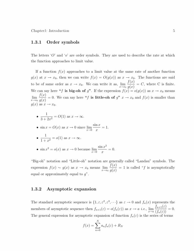
1.3.1 Order symbols

The letters ‘O’ and ‘o’ are order symbols. They are used to describe the rate at which

the function approaches to limit value.

If a function f(x) approaches to a limit value at the same rate of another function

g(x) at x → x0, then we can write f(x) = O(g(x)) as x → x0. The functions are said

to be of same order as x → x0. We can write it as, limx→x0

f(x)

g(x)= C, where C is finite.

We can say here “f is big-oh of g”. If the expression f(x) = o(g(x)) as x → x0 means

limx→x0

f(x)

g(x)= 0. We can say here “f is little-oh of g” x → x0 and f(x) is smaller than

g(x) as x → x0.

• 1

3 + 2x2= O(1) as x →∞.

• sin x = O(x) as x → 0 since limx→0

sin x

x= 1.

• 1

1 + x2= o(1) as x →∞.

• sin x2 = o(x) as x → 0 because limx→0

sin x2

x= 0.

“Big-oh” notation and “Little-oh” notation are generally called “Landau” symbols. The

expression f(x) ∼ g(x) as x → x0 means limx→x0

f(x)

g(x)= 1 is called “f is asymptotically

equal or approximately equal to g”.

1.3.2 Asymptotic expansion

The standard asymptotic sequence is {1, ε, ε2, ε3, · · ·} as ε → 0 and fn(x) represents the

members of asymptotic sequence then fn+1(ε) = o(fn(ε)) as x → a i.e., limx→a

fn+1(ε)

(fn(ε))= 0.

The general expression for asymptotic expansion of function fn(ε) is the series of terms

f(x) =N∑

n=0

anfn(ε) + RN

6

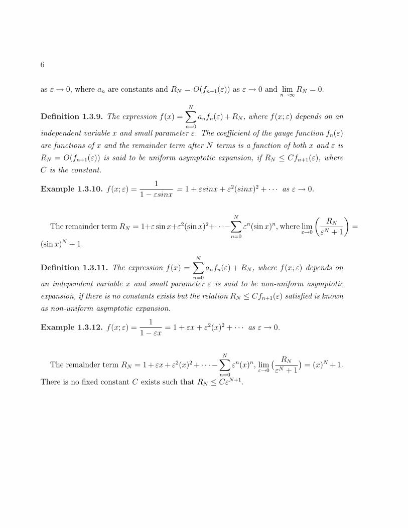
as ε → 0, where an are constants and RN = O(fn+1(ε)) as ε → 0 and limn→∞

RN = 0.

Definition 1.3.9. The expression f(x) =N∑

n=0

anfn(ε)+RN , where f(x; ε) depends on an

independent variable x and small parameter ε. The coefficient of the gauge function fn(ε)

are functions of x and the remainder term after N terms is a function of both x and ε is

RN = O(fn+1(ε)) is said to be uniform asymptotic expansion, if RN ≤ Cfn+1(ε), where

C is the constant.

Example 1.3.10. f(x; ε) =1

1− εsinx= 1 + εsinx + ε2(sinx)2 + · · · as ε → 0.

The remainder term RN = 1+ε sin x+ε2(sin x)2+· · ·−N∑

n=0

εn(sin x)n, where limε→0

(RN

εN + 1

)=

(sin x)N + 1.

Definition 1.3.11. The expression f(x) =N∑

n=0

anfn(ε) + RN , where f(x; ε) depends on

an independent variable x and small parameter ε is said to be non-uniform asymptotic

expansion, if there is no constants exists but the relation RN ≤ Cfn+1(ε) satisfied is known

as non-uniform asymptotic expansion.

Example 1.3.12. f(x; ε) =1

1− εx= 1 + εx + ε2(x)2 + · · · as ε → 0.

The remainder term RN = 1+ εx+ ε2(x)2 + · · ·−N∑

n=0

εn(x)n, limε→0

( RN

εN + 1

)= (x)N +1.

There is no fixed constant C exists such that RN ≤ CεN+1.

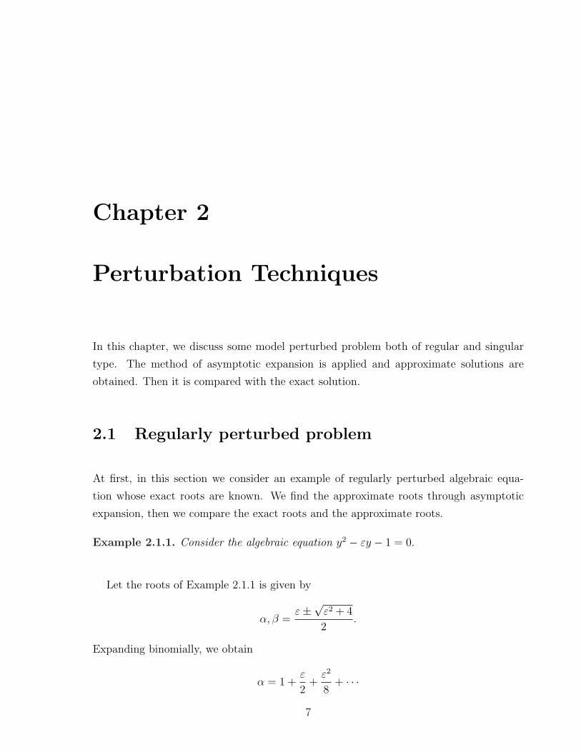
Chapter 2

Perturbation Techniques

In this chapter, we discuss some model perturbed problem both of regular and singular

type. The method of asymptotic expansion is applied and approximate solutions are

obtained. Then it is compared with the exact solution.

2.1 Regularly perturbed problem

At first, in this section we consider an example of regularly perturbed algebraic equa-

tion whose exact roots are known. We find the approximate roots through asymptotic

expansion, then we compare the exact roots and the approximate roots.

Example 2.1.1. Consider the algebraic equation y2 − εy − 1 = 0.

Let the roots of Example 2.1.1 is given by

α, β =ε±√ε2 + 4

2.

Expanding binomially, we obtain

α = 1 +ε

2+

ε2

8+ · · ·

7

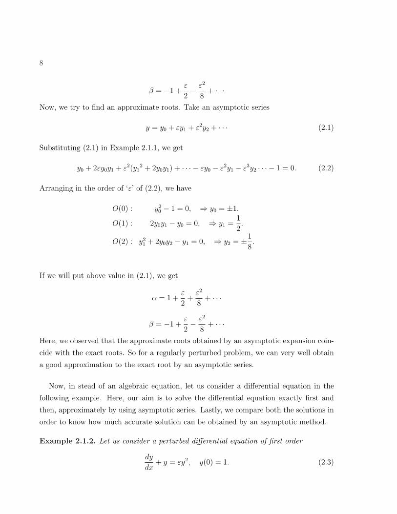
8

β = −1 +ε

2− ε2

8+ · · ·

Now, we try to find an approximate roots. Take an asymptotic series

y = y0 + εy1 + ε2y2 + · · · (2.1)

Substituting (2.1) in Example 2.1.1, we get

y0 + 2εy0y1 + ε2(y12 + 2y0y1) + · · · − εy0 − ε2y1 − ε3y2 · · · − 1 = 0. (2.2)

Arranging in the order of ‘ε’ of (2.2), we have

O(0) : y20 − 1 = 0, ⇒ y0 = ±1.

O(1) : 2y0y1 − y0 = 0, ⇒ y1 =1

2.

O(2) : y21 + 2y0y2 − y1 = 0, ⇒ y2 = ±1

8.

If we will put above value in (2.1), we get

α = 1 +ε

2+

ε2

8+ · · ·

β = −1 +ε

2− ε2

8+ · · ·

Here, we observed that the approximate roots obtained by an asymptotic expansion coin-

cide with the exact roots. So for a regularly perturbed problem, we can very well obtain

a good approximation to the exact root by an asymptotic series.

Now, in stead of an algebraic equation, let us consider a differential equation in the

following example. Here, our aim is to solve the differential equation exactly first and

then, approximately by using asymptotic series. Lastly, we compare both the solutions in

order to know how much accurate solution can be obtained by an asymptotic method.

Example 2.1.2. Let us consider a perturbed differential equation of first order

dy

dx+ y = εy2, y(0) = 1. (2.3)

Perturbation Expansion 9

Solving exactly, we havedy

dx+ y = εy2 =⇒ dy

dx= εy2 − y =⇒

∫1

y(εy − 1)dy =

∫dx.

Now using partial fraction

1

y(εy − 1)=

A

y+

B

(εy − 1)=⇒ 1

y(εy − 1)=

y(Aε + B)− A

y(εy − 1). (2.4)

Comparing both the sides, we get A = −1 and B = ε. Putting the value of A and B in

(2.4) and integrating, we obtainεy − 1

y= Cex. (2.5)

Applying initial condition, we getεy − 1

y= (ε− 1)ex. Simplifying, we have

y = e−x + ε(e−x − e−2x) + ε2(e−x − e−2x + e−3x) + · · · (2.6)

which is the exact solution of (2.3).

Now, we wish to find an approximate solution. Let us take an asymptotic series depends

on independent variable x and small parameter ε is given by

y = y0 + εy1 + ε2y2 + · · · (2.7)

Substituting (2.7) in (2.3), we get

dy0

dx+ ε

dy1

dx+ ε2dy2

dx+ · · ·+ y0 + εy1 + ε2y2 + · · · = ε(y0 + εy1 + ε2y2 + · · · )2. (2.8)

and initial condition can be written as

y0 + εy1 + ε2y2 + · · · = 1 + 0ε + 0ε2 · · · (2.9)

Arranging in the order of ‘ε’ of (2.8), we get the following system of differential equations:

O(1) :dy0

dx+ y0 = 0, y0(0) = 1. (2.10)

O(ε) :dy1

dx+ y1 = y2

0, y1(0) = 0. (2.11)

O(ε2) :dy2

dx+ y2 = 2y0y1, y2(0) = 0. (2.12)

Solving (2.10), we obtain y0 = C1e−x. Using the initial condition y0(0) = 1, we get

y0 = e−x. Solving (2.11), we obtain y1 = C2e−x − e−2x and using the initial condition

10

y1(0) = 0, we get y1 = e−x − e−2x.

Solving (2.12), we obtain y2 = C3e−x − 2e−2x + e−3x and using the initial condition

y2(0) = 0, we get y2 = e−x − 2e−2x + e−3x.

Substituting the value of y0, y1, y2 in (2.7), we have

y = e−x + ε(e−x − e−2x) + ε2(e−x − 2e−2x + e−3x) + · · · (2.13)

Here, we observed from the above example that the exact solution of (2.3) given by (2.6)

and approximate solution given by (2.13) are very well matching. The problem (2.3) is a

regularly perturbed differential equation. Also, if we put ε = 0, the (2.3) becomes

dy

dx+ y = 0. (2.14)

Comparing (2.3) and (2.14), one can easily observe that the order of the perturbed dif-

ferential equation and unperturbed differential equation are same.

2.2 Singularly perturbed problem

In the previous section, we have discussed an algebraic and one differential equation

involving ε and both are of regularly perturbed type. Now in this section, we consider

an algebraic equation and differential equation involving small parameter, both are of

singularly perturbed nature. We will solve these problems through the above procedure

to get the behavior singular perturbation.

Example 2.2.1. Let us consider an algebraic equation

εx2 − x + 1 = 0. (2.15)

The roots of (2.15) is given by

α, β =1±√1− 4ε

2ε.

α =1

ε− 1− ε− · · ·

Perturbation Expansion 11

β = 1 + ε + ε2 + · · ·which are the two exact roots of (2.15). Let us consider an asymptotic series

x = x0 + εx1 + ε2x2 + · · · (2.16)

Substituting (2.16) in (2.15), we get

ε(x0 + εx1 + ε2x2 + · · · )2 − (x0 + εx1 + ε2x2 + · · · ) + 1 = 0. (2.17)

Arranging in the order of ε of (2.17), we get the following system of equations:

O(0) : −x0 + 1 = 0, ⇒ x0 = 1.

O(1) : x20 − x1 = 0, ⇒ x1 = 1.

O(2) : 2x0x1 − x2 = 0, ⇒ x2 = 2.

Now putting the value of x0, x1, x2 in the (2.16), we get

x = 1 + ε + 2ε + 2ε2 + · · · , (2.18)

which matches to the solved root β up to two terms of the asymptotic expansion. So,

we can get only one approximate root through asymptotic expansion. The other root α

can not be approximated. So for singularly perturbed problem, we can not get a good

approximation to the exact roots by one term asymptotic series.

Now, in stead of an algebraic equation, let us consider differential equations in the

following examples. Here, our aim is to solve the differential equation exactly and then,

approximately by using asymptotic series. Finally, we compare both the solutions in order

to know how much accurate solutions can be obtained by the asymptotic method.

Example 2.2.2. Consider a differential equation

εd2y

dx2+

dy

dx− y = 0, y(0) = 0, y(1) = 1. (2.19)

Solving exactly and applying the boundary conditions, we obtain

y =em1x − em2x

em1 − em2

12

which is the solution of (2.19), where m1,2 =−1±√1 + 4ε

2ε.

Let us take an asymptotic series

y = y0 + εy1 + ε2y2 + · · · (2.20)

Substituting (2.20) in (2.19), we get

ε(d2y0

dx2+ ε

d2y1

dx2+ ε2d2y2

dx2+ · · · )+ (

dy0

dx+ ε

dy1

dx+ ε2dy2

dx+ · · · )+ (y0 + εy1 + ε2y2 + · · · ) = 0.

(2.21)

Arranging in the order of ε of (2.21), we get the following system of differential equations:

O(0) :dy0

dx− y0 = 0, y0(0) = 0, y0(1) = 1. (2.22)

O(1) :dy1

dx+ y1 = −d2y0

dx2, y1(0) = 0, y1(1) = 0. (2.23)

Solving (2.22), we obtain

y0(x) = Cex. (2.24)

From the condition y0(0) = 0 and y0(1) = 1, we get y0(x) = 0 and y0 = ex−1 respectively.

Now the function y0(x) = 0 does not satisfy the condition at x = 1 and the function

y0 = e(x−1) does not satisfy the condition at x = 0 i.e., the solution fails to satisfy one of

the boundary condition. Again, we take ε = 0 in differential equation then, we get a first

order differential equationdy

dx+ y = 0. (2.25)

Where the order of perturbed differential equation (2.19) and the unperturbed differential

equation (2.25) are different. We conclude here by comparing both the solution that, we

cannot get a good approximation to the exact solution by one term asymptotic series.

Example 2.2.3. Let us consider the boundary value problem

εd2y

dx2+ (1 + ε)

dy

dx+ y = 0, y(0) = 0, y(1) = 1. (2.26)

Solving exactly, we get y = c3e−x+c4e

−xε using boundary condition. Applying boundary

condition, we get

y =e−x − e

−xε

e−1 − e−1ε

Perturbation Expansion 13

which the solution of (2.26).

Let us take an asymptotic series,

y = y0 + εy1 + ε2y2 + · · · (2.27)

Substituting (2.27) in (2.26), we get

ε(d2y0

dx2+ ε

d2y1

dx2+ ε2d2y2

dx2+ · · · ) + (

dy0

dx+ ε

dy1

dx+ · · · (2.28)

ε2dy2

dx+ · · · ) + (ε

dy0

dx+ ε2dy1

dx+ ε3dy2

dx+ · · · ) + (y0 + εy1 + ε2y2 + · · · ) = 0.

Arranging in the order of ε of (2.28), we get the following system of differential equation:

O(0) :dy0

dx+ y0 = 0, y0(0) = 0, y0(1) = 1. (2.29)

O(1) :dy1

dx+ y1 = −d2y0

dx2− dy0

dx, y1(0) = 0, y1(1) = 0. (2.30)

Solving (2.29), we have

y0(x) = Cex. (2.31)

Here, with one arbitrary constant both the boundary conditions cannot be satisfied. We

conclude here that we cannot get a good approximation to the exact solution for a singu-

larly perturbed problem by one term asymptotic expansion.

From the above examples, it is observed that the asymptotic expansion technique gives

approximate solution which matches well to the exact solution for problem of regularly

perturbed type. But at the same time, perturbation expansion does not provide a good

approximation for singularly perturbed problems. In order to obtain a fitted approxima-

tion for singularly perturbed problems, one can use the method of matched asymptotic

expansion which is discussed in the next section.

2.3 Matched asymptotic expansion

The method of matched asymptotic expansion was introduced by Ludwig Prandtl’s bound-

ary layer theory, in 1905. Mathematically, boundary layer occurs when small parameter is

14

multiplying with highest derivative of differential equation which is of singularly perturbed

in nature. Depending upon the presence of boundary layer, the domain of the problem

can be divided into two regions, first one is the outer region away from the boundary

layer where the solution behaves smoothly and second one is the inner region where the

gradient of the solution changes rapidly.

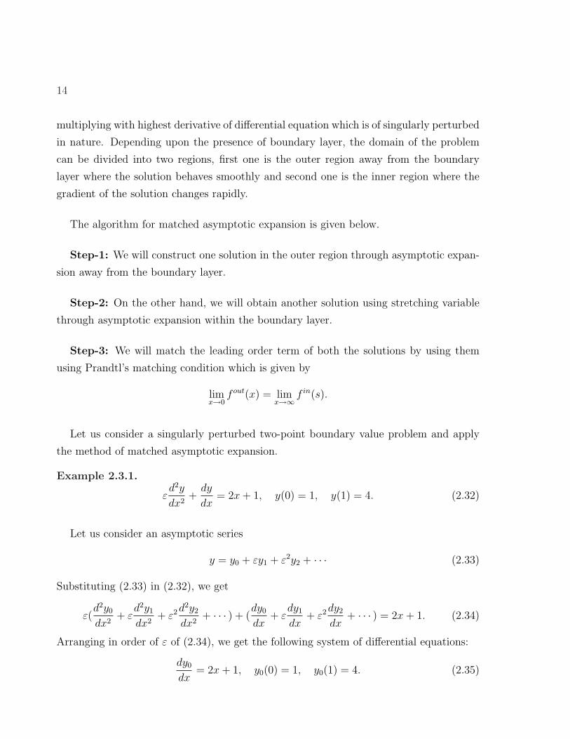
The algorithm for matched asymptotic expansion is given below.

Step-1: We will construct one solution in the outer region through asymptotic expan-

sion away from the boundary layer.

Step-2: On the other hand, we will obtain another solution using stretching variable

through asymptotic expansion within the boundary layer.

Step-3: We will match the leading order term of both the solutions by using them

using Prandtl’s matching condition which is given by

limx→0

f out(x) = limx→∞

f in(s).

Let us consider a singularly perturbed two-point boundary value problem and apply

the method of matched asymptotic expansion.

Example 2.3.1.

εd2y

dx2+

dy

dx= 2x + 1, y(0) = 1, y(1) = 4. (2.32)

Let us consider an asymptotic series

y = y0 + εy1 + ε2y2 + · · · (2.33)

Substituting (2.33) in (2.32), we get

ε(d2y0

dx2+ ε

d2y1

dx2+ ε2d2y2

dx2+ · · · ) + (

dy0

dx+ ε

dy1

dx+ ε2dy2

dx+ · · · ) = 2x + 1. (2.34)

Arranging in order of ε of (2.34), we get the following system of differential equations:

dy0

dx= 2x + 1, y0(0) = 1, y0(1) = 4. (2.35)

Perturbation Expansion 15

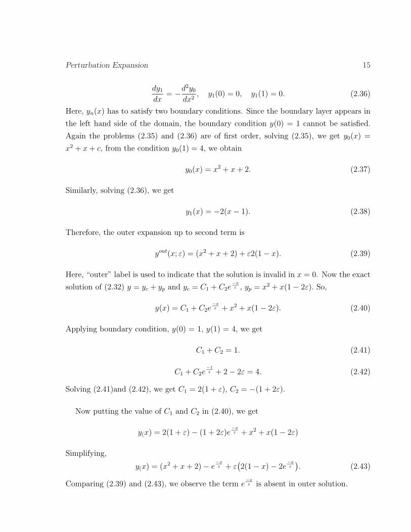
dy1

dx= −d2y0

dx2, y1(0) = 0, y1(1) = 0. (2.36)

Here, yn(x) has to satisfy two boundary conditions. Since the boundary layer appears in

the left hand side of the domain, the boundary condition y(0) = 1 cannot be satisfied.

Again the problems (2.35) and (2.36) are of first order, solving (2.35), we get y0(x) =

x2 + x + c, from the condition y0(1) = 4, we obtain

y0(x) = x2 + x + 2. (2.37)

Similarly, solving (2.36), we get

y1(x) = −2(x− 1). (2.38)

Therefore, the outer expansion up to second term is

yout(x; ε) = (x2 + x + 2) + ε2(1− x). (2.39)

Here, “outer” label is used to indicate that the solution is invalid in x = 0. Now the exact

solution of (2.32) y = yc + yp and yc = C1 + C2e−xε , yp = x2 + x(1− 2ε). So,

y(x) = C1 + C2e−xε + x2 + x(1− 2ε). (2.40)

Applying boundary condition, y(0) = 1, y(1) = 4, we get

C1 + C2 = 1. (2.41)

C1 + C2e−1ε + 2− 2ε = 4. (2.42)

Solving (2.41)and (2.42), we get C1 = 2(1 + ε), C2 = −(1 + 2ε).

Now putting the value of C1 and C2 in (2.40), we get

y(x) = 2(1 + ε)− (1 + 2ε)e−xε + x2 + x(1− 2ε)

Simplifying,

y(x) = (x2 + x + 2)− e−xε + ε

(2(1− x)− 2e

−xε

). (2.43)

Comparing (2.39) and (2.43), we observe the term e−xε is absent in outer solution.

16

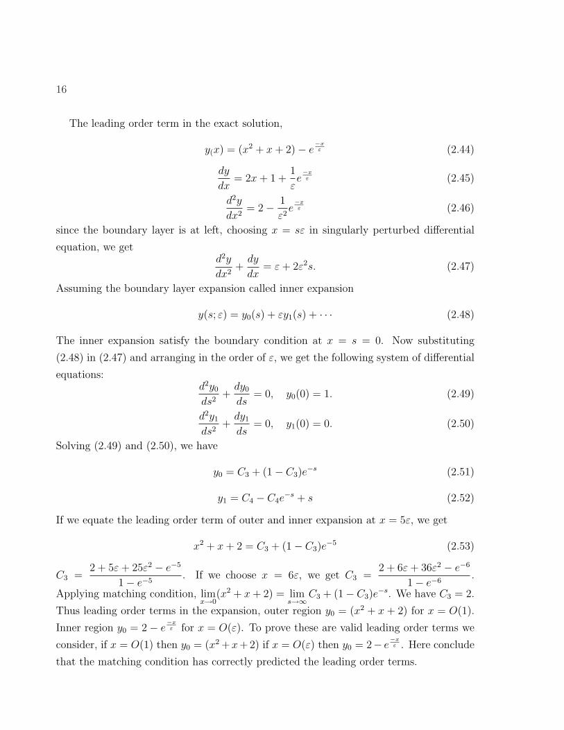
The leading order term in the exact solution,

y(x) = (x2 + x + 2)− e−xε (2.44)

dy

dx= 2x + 1 +

1

εe−xε (2.45)

d2y

dx2= 2− 1

ε2e−xε (2.46)

since the boundary layer is at left, choosing x = sε in singularly perturbed differential

equation, we getd2y

dx2+

dy

dx= ε + 2ε2s. (2.47)

Assuming the boundary layer expansion called inner expansion

y(s; ε) = y0(s) + εy1(s) + · · · (2.48)

The inner expansion satisfy the boundary condition at x = s = 0. Now substituting

(2.48) in (2.47) and arranging in the order of ε, we get the following system of differential

equations:d2y0

ds2+

dy0

ds= 0, y0(0) = 1. (2.49)

d2y1

ds2+

dy1

ds= 0, y1(0) = 0. (2.50)

Solving (2.49) and (2.50), we have

y0 = C3 + (1− C3)e−s (2.51)

y1 = C4 − C4e−s + s (2.52)

If we equate the leading order term of outer and inner expansion at x = 5ε, we get

x2 + x + 2 = C3 + (1− C3)e−5 (2.53)

C3 =2 + 5ε + 25ε2 − e−5

1− e−5. If we choose x = 6ε, we get C3 =

2 + 6ε + 36ε2 − e−6

1− e−6.

Applying matching condition, limx→0

(x2 + x + 2) = lims→∞

C3 + (1− C3)e−s. We have C3 = 2.

Thus leading order terms in the expansion, outer region y0 = (x2 + x + 2) for x = O(1).

Inner region y0 = 2− e−xε for x = O(ε). To prove these are valid leading order terms we

consider, if x = O(1) then y0 = (x2 +x+2) if x = O(ε) then y0 = 2− e−xε . Here conclude

that the matching condition has correctly predicted the leading order terms.

Chapter 3

Conclusion and Future work

3.1 Conclusion

In this thesis, we have discussed the application of asymptotic expansion method for some

model problems involving small parameter ε. In Chapter 1, we have defined some basic

terminologies, definition of regular and singular perturbation, Landau symbols, uniform

and non-uniform asymptotic expansions. In Chapter 2, at first we have applied the method

of asymptotic expansion for some model algebraic equations and differential equations

containing ε. Then, we have applied the same method on some model singularly perturbed

problems. We have observed that the asymptotic expansion method gives very good

result for regularly perturbed problems where as one term asymptotic expansion does not

work well for singularly perturbed problems. To get a good approximation for singularly

perturbed problems, the method of matched asymptotic expansion is discussed in the last

section of Chapter 2 and we conclude that through matched asymptotic expansion, one

can obtain a good approximation for singularly perturbed problems.

17

18

3.2 Future work

The work of the thesis can be extended in various directions. Some of the future works

to be carried out are listed below.

1. The problems considered here are linear one dimensional problems. One can also

extend the idea of asymptotic expansion discussed here to problems in higher dimen-

sion. It can also be extended for non-linear differential equation which is difficult

to solve exactly.

2. The solution obtained through asymptotic expansion gives us an awareness of the

exact solution before solving the problem analytically or numerically. So, one can

get some idea about the solution of perturbation problems through asymptotic ex-

pansion before solving it.

Bibliography

[1] A.B. Bush. Perturbation Methods for Engineers and Scientists. CRC Press, Boca

Raton, 1992.

[2] M.H. Holmes. Introduction to Perturbation Methods. Springer Verlag, Heidelbers,

1995.

[3] J. Kevorkian and J.D. Cole. Perturbation Methods in Applied Mathematics. Springer

Verlag, Heidelbers, 1981.

[4] J.D. Logan. Applied Mathematics. John Wiley and Sons, New York, 2006.

[5] J.A. Murdock. Perturbation Theory and Methods. John Wiley and Sons, New York,

1991.

[6] A.H. Nayfeh. Introduction to Perturbation Techniques. John Wiley and Sons, New

York, 1993.

[7] R.E. O’Malley. Singular Perturbation Methods for Ordinary Differential Equations.

Springer Verlag, Heidelbers, 1991.

19