Embed Size (px)
Citation preview
Asymptotic Expansions of Empirical Likelihood in Time
Series LIU, Li
A Thesis Submitted in Partial Fulfilment of the Requirements for the Degree of
Master of Philosophy in
Statistics June 2009
P ( 1 5 F E B J l l _ _ i
mVllNlVf,lsiTY"一J磨I
Thesis/Assessment Committee
Professor LEUNG PUI LAM (Chair)
Professor CHAN NGAI HANG (Thesis Supervisor)
Professor GU MING GAO (Committee Member)
Professor KENICHIRO TAMAKI (External Examiner)
THE CHINESE UNIVERSITY OF HONG KONG G R A D U A T E SCHOOL
The undersigned certify that we have read a thesis, entitled "Asymptotic Expansion of Empirical Likelihood in Time Series" submitted to the Graduate School by LIU, Li in partial fulfilment of the requirements for the degree of Master of Philosophy in Statistics. We recommend that it be accepted.
Prof. Ngai-Han Chan Supervisor
Prof. Ming Gao Gu
Prof. Pui Lam Leung
Prof. Kenichiro Tamaki External Examiner
i

DECLARATION
No portion of the work referred to in this thesis has been submitted in support of an application for another degree or qualification of this or any other university or other institution of learning.
ii

ACKNOWLEDGEMENT
I would like to thank my supervisor, Prof. Chan Ngai Hang, for his invalu-able guidance and helpful assistance, without which the completion of this thesis would not have been possible. I am also sincerely grateful for his teaching, en-couragement, and patience throughout the researching and writing of this thesis, which helped me to overcome so many obstacles. I also acknowledge my fellow classmates and the staff at the Department of Statistics for their kind assistance.
I thank Prof. Tamaki for his valuable help and for his patient and detailed replies to my questions. I am also grateful to Mr. Yau Chun Yip for his helpful advices and for spending time with me to discuss my research.
iii
Abstract of thesis entitled: . Asymptotic Expansions of Empirical Likelihood in Time Series Submitted by Liu Li for the degree of Master of Philosophy in Statistics at The Chinese University of Hong Kong in May 2009.
A B S T R A C T
This thesis considers asymptotic expansions of empirical likelihood (EL) in time series. The validity of the formal Edgeworth expansion for the EL ratio sta-tistic in the short-memory case is established and through lengthy and onerous calculations a closed form of Edgeworth expansion for the statistic is deduced. It is demonstrated that the coverage error of the EL confidence region for time series is of the order 0 ( l / n ) , where n is the sample size. It is further shown that the coverage error can be reduced to o(l /n) by using a Bartlett correction. A simulation study is presented to illustrate the Bartlett correction for EL in the short-memory case.
iv

摘要
本論文研究時間序列經驗似然的漸進分佈。首先,在短記憶時
間序列情況下,我們證明了經驗似然比統計量的埃奇沃思展開的正確
性。緊接着,經過大量的推導計算,我們得到了經驗似然比統計量的
埃奇沃思展開的表達式。根據這個表達式可以證明時間序列經驗似然
的置信區間的誤差階為 0 ( l / n),其中 n代録樣本量。我們進一步證
明,通過巴特萊特糾正,時間序列經驗似然的置信區間的誤差階可以
被減小至 o ( l / n ) �最后,我們通過實驗論證了在短記憶時間序列的情
況下,時間序列經驗似然服從巴特萊特糾正。
V

Contents
1 Introduction 1 1.1 Empirical Likelihood 1 1.2 Empirical Likelihood for Dependent Data 4
1.2.1 Spectral Method 5 1.2.2 Blockwise Method g
1.3 Edgeworth Expansions and Bartlett Correction 9 1.3.1 Coverage Errors 10 1.3.2 Edgeworth Expansions 11 1.3.3 Bartlett Correction 13
2 Bartlett Correction for EL 2.1 Empirical Likelihood in Time Series 16 2.2 Stochastic Expansions of EL in Time Series 19 2.3 Edgeworth Expansions of EL in Time Series 22
2.3.1 Validity of the Formal Edgeworth Expansions 22 2.3.2 Cumulant Calculations 24
2.4 Main Results
3 Simulations 32 3.1 Confidence Region 33 3.2 Coverage Error of Confidence Regions 35
vi

4 Conclusion and Future Work 38
Bibliography 41
.—-
vii
List of Figures 3.1 95% empirical likelihood confidence region (solid line), Bartlett
corrected empirical likelihood confidence region (dotted line) and the true value of parameters (cross point) 37
viii
Chapter 1
Introduction
1.1 Empirical Likelihood Empirical likelihood (EL), as discussed by Owen (1988’ 1990), is a nonparametric
approach of statistical inference that allows data analysts to use a likelihood
method without having to assume that the data come from a known distribution.
It thus combines the reliability of the nonparametric method and the effectiveness
of the likelihood approach.
Let be independent observations from a distribution Fq with a
mean /i and a nonsingular covariance matrix. The EL function L{F) can be
defined as: n n
L(F) = n inXi) — F(x~)) = Hp,. (1.1) t=l i=l
where Pi 二 - F ( X i - ) . Equation (1.1) is maximized by the empirical
cumulative distribution function (ECDF) (Owen, 2001’ Theorem 2.1), which is
1
defined as:
Fn{x) = -J2l{Xi<x), 1=1
where I{X < x) is the indicator function. Analogous to the parametric likelihood
method, the EL ratio can be written as
R{F) = L(F)/max{L(F)} = L(F) /L(F . ) n 打 1 打
= ( 1 2 ) z=l i=l i=l Note that Xi are not required to be distinct here or anywhere else.
Consider a p-dimensional parameter 9 associated with Fq and a vector-valued
function m{X, 9) G iT. Suppose that
E(m(X,6l)) = 0.
To conduct inference for 0 using the EL approach, the profile EL ratio function
for 0 is defined as: n n n
R{0) = s u p i H ^ P i b i > 0 , J 2 p i = l , J2p im{Xi , e ) = 0}, t=l t=l i=zl which means maximizing (1.2) subject to the restrictions
n ( 1 ) =
. i=l n
(2) [ P i = l’ i=l
(3) Pi > 0.
As noted by Qin and Lawless (1994), for a given 9, the maximum exists, provided
that 0 is interior to the convex hull of the points m{Xi,0), ...,m(Xn,0). This
2
maximum can be found by using a Lagrange multiplier argument. Let n n n
H(vu …’Pn,i,7) = ^lognpi + t ( l - Y ^ P i ) -i=l i i
where t and 7 = (71’...’7s)了 are Lagrange multipliers. Taking derivatives with
respect to pi gives
8H 1
_ = = (1.3)
since pi > 0, this gives 1 -印i - nj^Pim(Xi, 7) = 0. (1.4)
Summing (1.4) from i 二 1 to n and using restrictions (1) and (2) leads to t = n.
Substituting t = n into (1.3) gives
— i 1
灼 = G . 1 + 7"M不’約. ( 1 . 5 )
From (1.5) and restriction (1), the following equation are obtained as the solution
to 7 :
+ (1.6) Z—1
Let De = { j : I + 7了m(Xi’ 没)> 1/n}’ De is convex and closed for fixed 6 and
is bounded if 0 is interior to the convex hull of the points m(Xi, 9), 9).
As is positive definite,
a i ^ p mjXue)
3
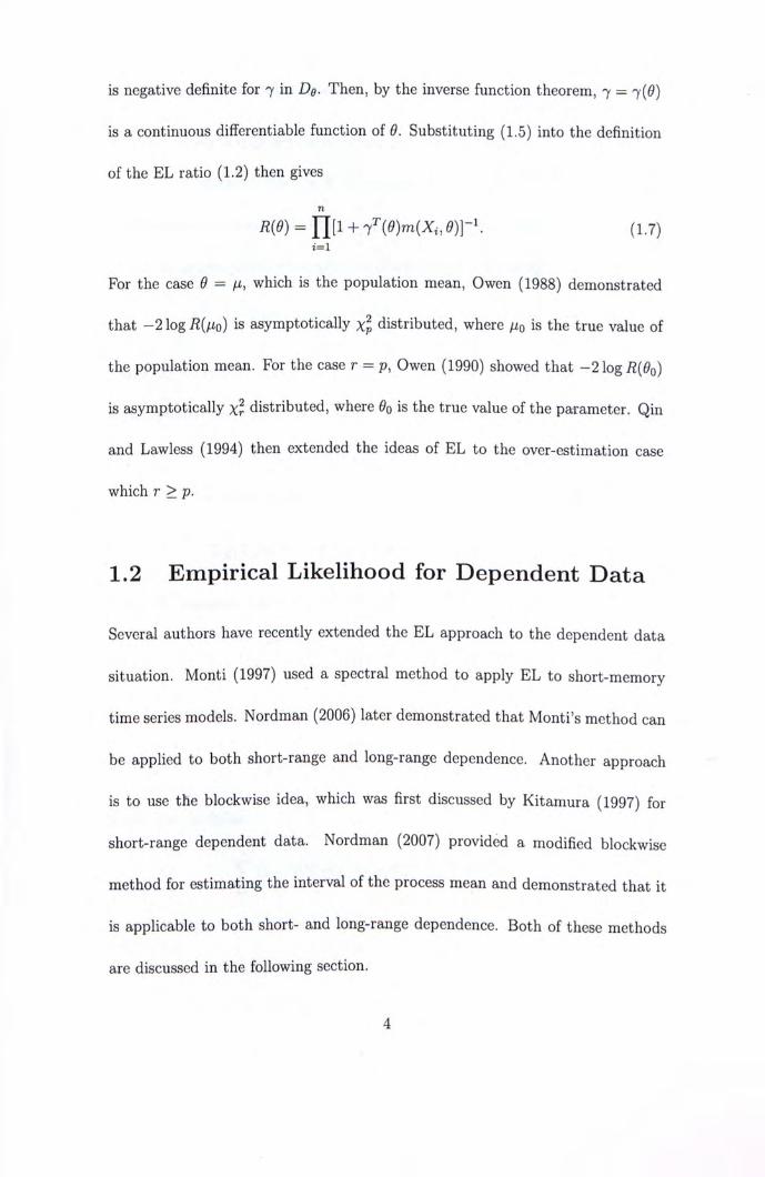
is negative definite for 7 in Dg. Then, by the inverse function theorem, 7 = 7(0)
is a continuous differentiable function of 9. Substituting (1,5) into the definition
of the EL ratio (1.2) then gives n
R{e) = l l [ l + j^(9)m{X,,9)]- \ (1.7) i=l
For the case 9 = fi, which is the population mean, Owen (1988) demonstrated
that -21ogi?("o) is asymptotically Xp distributed, where "0 is the true value of
the population mean. For the case r = p, Owen (1990) showed that - 2 log R{9Q)
is asymptotically xl distributed, where Oq is the true value of the parameter. Qin
and Lawless (1994) then extended the ideas of EL to the over-estimation case
which r >p.
1.2 Empirical Likelihood for Dependent Data Several authors have recently extended the EL approach to the dependent data
situation. Monti (1997) used a spectral method to apply EL to short-memory
time series models. Nordman (2006) later demonstrated that Monti's method can
be applied to both short-range and long-range dependence. Another approach
is to use the blockwise idea, which was first discussed by Kitamura (1997) for
short-range dependent data. Nordman (2007) provided a modified blockwise
method for estimating the interval of the process mean and demonstrated that it
is applicable to both short- and long-range dependence. Both of these methods
are discussed in the following section.
4
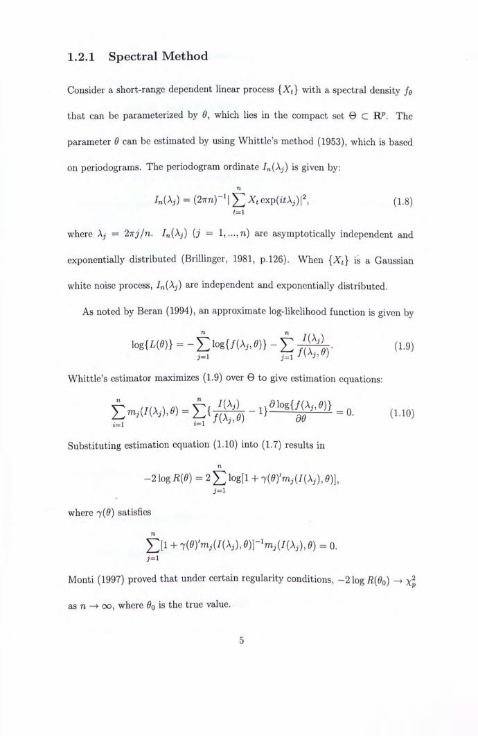
1.2.1 Spectral Method
Consider a short-range dependent linear process { X J with a spectral density fe
that can be parameterized by 9, which lies in the compact set 0 C R^. The
parameter 9 can be estimated by using Whittle's method (1953), which is based
on periodograms. The periodogram ordinate /^(Aj) is given by: n
IniXj) = {27rn)-'\Y,Xtexp{itXj)\ ' , (1.8) t=i
where Xj = 2iTj/n. /„(Aj) {j = l’...’n) are asymptotically independent and
exponentially distributed (Brillinger, 1981’ p.l26). When {Xt} is a Gaussian
white noise process, Ini^j) are independent and exponentially distributed.
As noted by Beran (1994), an approximate log-likelihood function is given by
\og{L(e)} = (1.9) j=i j=i 八 〜 ’ "J
Whittle's estimator maximizes (1.9) over 6 to give estimation equations:
’一 = (1.10)
Substituting estimation equation (1.10) into (1.7) results in n
一2 log R(6) = 2 ^ log[l + 6)],
where j{9) satisfies n
+ l{Oymj{I{\j), 9) = 0. j=i Monti (1997) proved that under certain regularity conditions, 一21ogi?(0o) — Xp
as n —> oo, where 9Q is the true value.
5
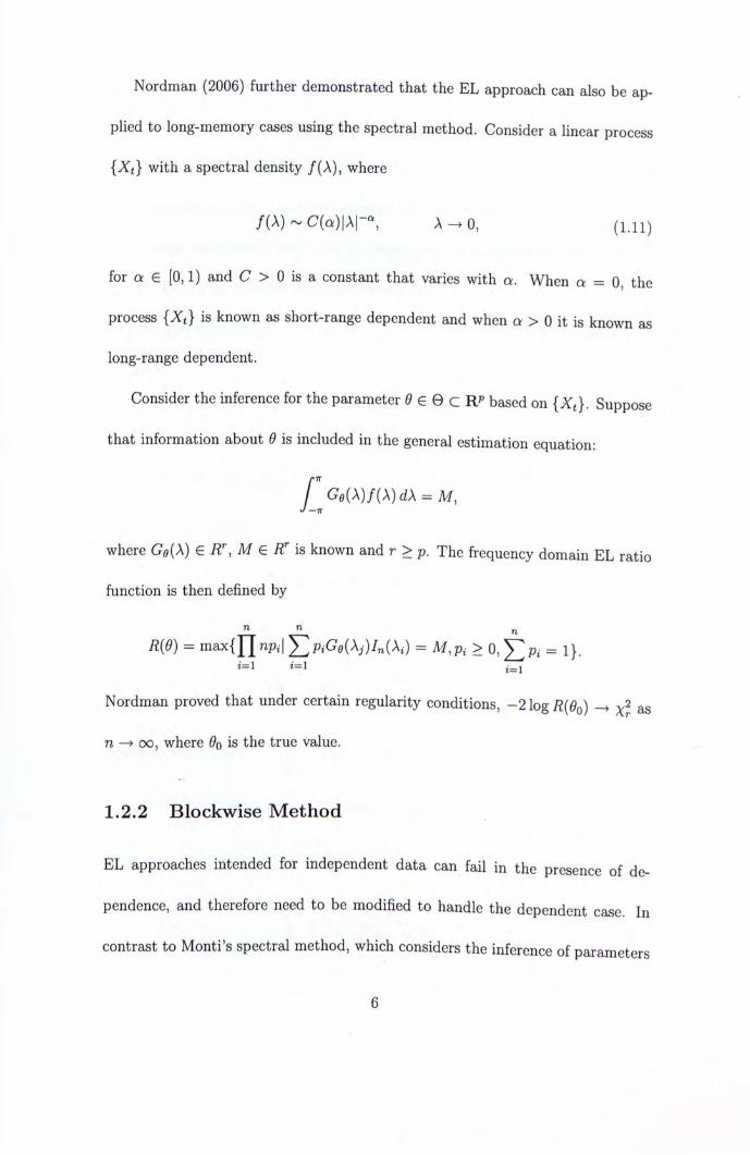
Nordman (2006) further demonstrated that the EL approach can also be ap-
plied to long-memory cases using the spectral method. Consider a linear process
{ X J with a spectral density /(A), where
/ ( A ) � C V ) | A | - � A —0’ (1.11)
for a e [0,1) and C > 0 is a constant that varies with a. When a = 0’ the
process { X J is known as short-range dependent and when a > 0 it is known as
long-range dependent.
Consider the inference for the parameter 0 e 6 C Rp based on { ^ J . Suppose
that information about 6 is included in the general estimation equation:
[Ge{X)f{\)d\ = M, J —TT
where Ge[\) e R\ M E /T is known and r > p. The frequency domain EL ratio function is then defined by
n RW = max{J][npi| Y^PiGe{Xj)In{Xi) = M,pi > 0’ f p * = 1}.
i = l 1=1 i = i
Nordman proved that under certain regularity conditions, - 2 log R{eQ) ;朋
n — 00, where is the true value.
1.2.2 Blockwise Method
EL approaches intended for independent data can fail in the presence of de-
pendence, and therefore need to be modified to handle the dependent case. In
contrast to Monti's spectral method, which considers the inference of parameters
6
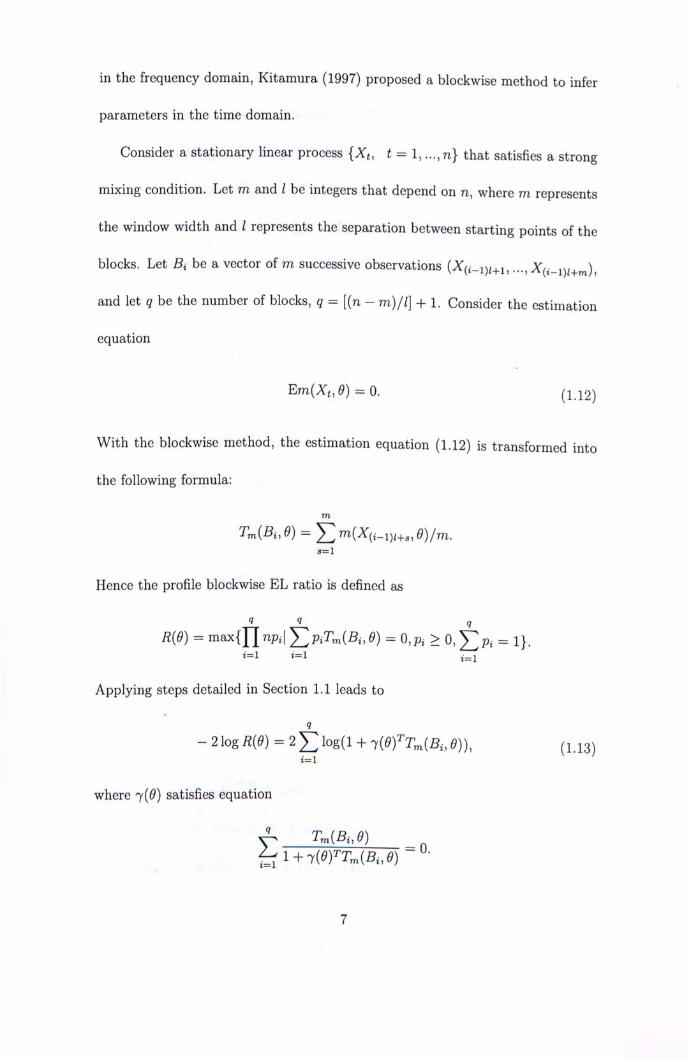
in the frequency domain, Kitamura (1997) proposed a blockwise method to infer
parameters in the time domain.
Consider a stationary linear process {Xt, t = l , . . . ,n} that satisfies a strong
mixing condition. Let m and I be integers that depend on n, where m represents
the window width and I represents the separation between starting points of the
blocks. Let Bi be a vector of m successive observations iXa i�,丄i ; r , . …、
\ 一•U【十1 ’ ...’ "• »"(t-l)i+my,
and let q be the number of blocks, q = [{n - m)/l] + 1. Consider the estimation
equation Em{Xt,e) = 0. (1.12)
With the blockwise method, the estimation equation (1.12) is transformed into
the following formula: m
S=1
Hence the profile blockwise EL ratio is defined as 9 9 q
m = m^x{ l \np i \ ^p iTr r , {B , ,9 ) = = 1}. i=i i=i i=i
Applying steps detailed in Section 1.1 leads to
- 2 log _ = 2 [ log(l + m ' ^ T m i B , , e ) l (1.13) i=l
where ^(6) satisfies equation
亡 Tm[Bi, 6)
7
Kitamura (1997) proved that under certain regularity conditions, log R{9)
is asymptotically chi-squared distributed, where An = q~^{n/m).
As an illustration, consider the inference of the process mean /i, in which the
estimation equation m{Xt, /u) = JQ - /i = 0 is used and the blockwise estimation
equation becomes Tm{Buii) = J27=i i^ii-i)i+s 一 Substituting this block-
wise estimation equation into (1.13) gives the log EL ratio for the process mean,
that is: q m
-2\ogR(fi) = 2 5 ] l o g [ l + 7 � • — ")]. (1.14) i = l s = l “
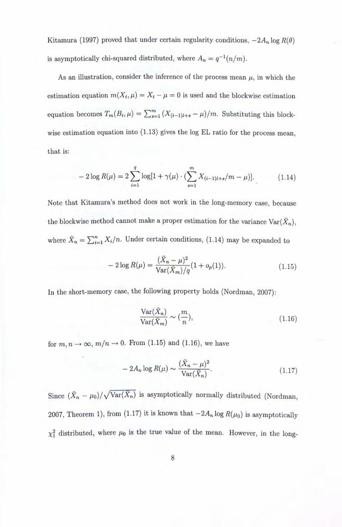
Note that Kitamura's method does not work in the long-memory case, because
the blockwise method cannot make a proper estimation for the variance Var(X„),
where Xn = I X i 不/几.Under certain conditions, (1.14) may be expanded to
- 21 遍 + 僅 _
In the short-memory case, the following property holds (Nordman, 2007):
Var(Xn) m (1.16)
for m ,n —> cxD, m/n — 0. From (1.15) and (1.16), we have
一 • 卜 ( 1 . 1 7 )
Since {Xn — "o) / \ /Var(Xi) is asymptotically normally distributed (Nordman,
2007’ Theorem 1), from (1.17) it is known that log/?(/io) is asymptotically
x j distributed, where /io is the true value of the mean. However, in the long-
8
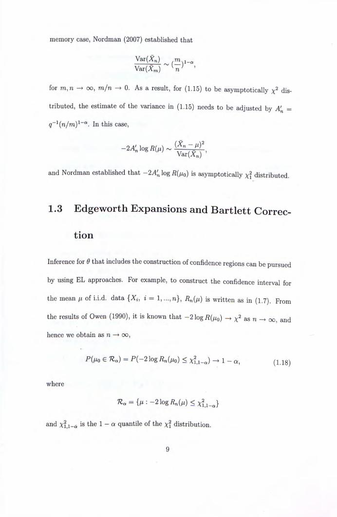
memory case, Nordman (2007) established that
V a r ( X ) 凸 i - a V a r ( X ^ ) � ’
for m,n oo, m/n — 0. As a result, for (1.15) to be asymptotically dis-
tributed, the estimate of the variance in (1.15) needs to be adjusted by A'=
q—乂n/mY—a. In this case,
and Nordman established that logi?(/xo) is asymptotically xf distributed.
1.3 Edgeworth Expansions and Bartlett Correc-tion
Inference for 0 that includes the construction of confidence regions can be pursued
by using EL approaches. For example, to construct the confidence interval for
the mean “ of i.i.d. data {Xi, i = l’...’n}’ is written as in (1.7). From
the results of Owen (1990), it is known that -21ogi?(/io) as n oo and
hence we obtain as n oo,
Pif^o e = P(-21ogi?„(/xo) < xh-J — 1 - a , (1.18)
where
and Xi,i-a is the 1 - a quantile of the Xi distribution.
9
Since - 2 log R n M is only asymptotically x j distributed, there is some cov-
erage error in the confidence interval for fi‘ In the following, the order of the
coverage error is discussed and Bartlett correction is proposed to reduce the cov-
erage error.
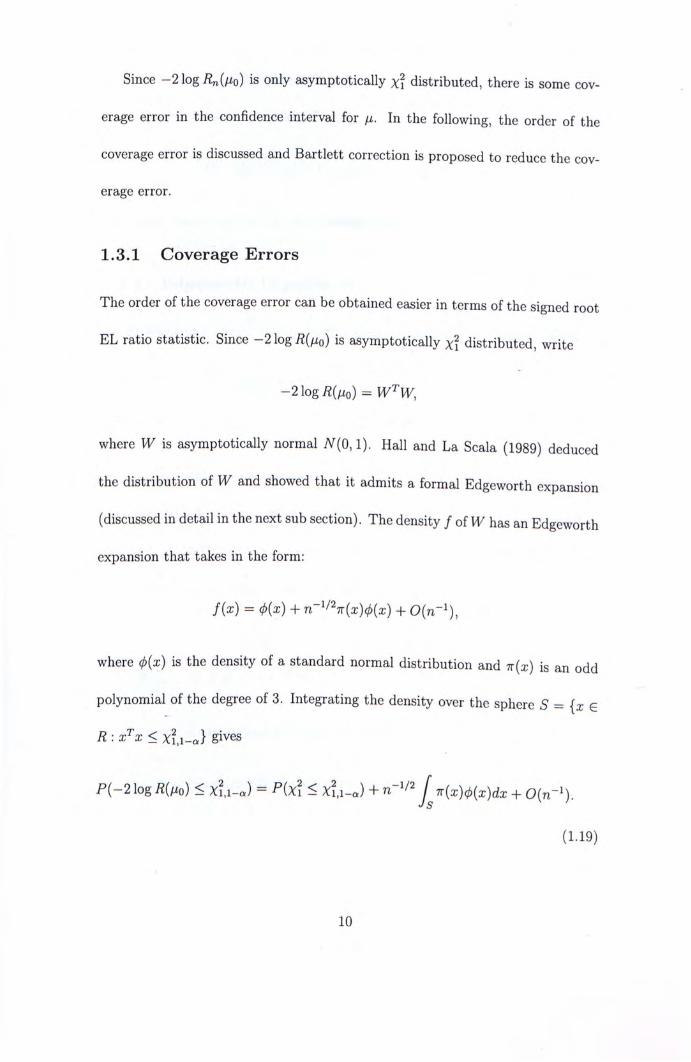
1.3.1 Coverage Errors
The order of the coverage error can be obtained easier in terms of the signed root
EL ratio statistic. Since —2 log i?(/io) is asymptotically Xi distributed, write
- 2 1 o g / ? ( " o ) = W ^ W ,
where is asymptotically normal iV(0’ 1). Hall and La Scala (1989) deduced
the distribution of W and showed that it admits a formal Edgeworth expansion
(discussed in detail in the next sub section). The density f oiW has an Edgeworth
expansion that takes in the form:
/(rr) = cj>(x) + n-'/'7T{x)cl>{x) + 0(71-1)’
where <p{x) is the density of a standard normal distribution and 7r(a:) is an odd
polynomial of the degree of 3. Integrating the density over the sphere S = {x e
R - . x ^ x < x?’i_cJ gives
P(-2\ogR(^lo) < xh-a) = P{x\ < X?’i-J + J^n{x)cf>{x)dx + 0(n—”.
(1.19)
10
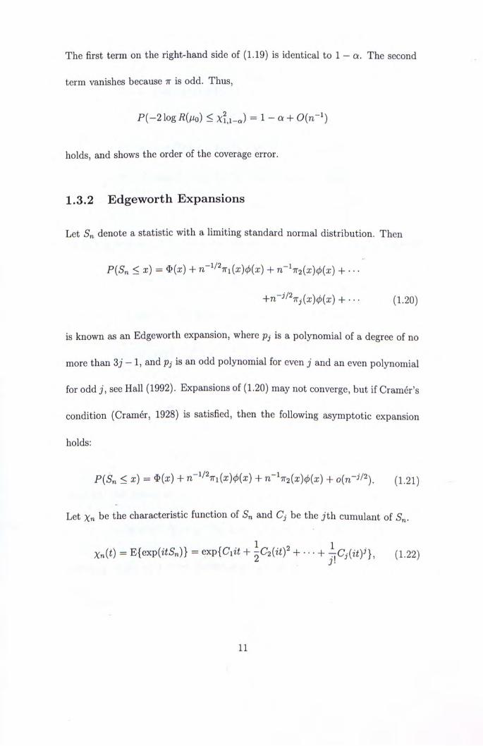
The first term on the right-hand side of (1.19) is identical to 1 - a. The second
term vanishes because tt is odd. Thus,
尸(一2 log Rifio) < X?,i-a) = 1 - c + 0(n—i)
holds, and shows the order of the coverage error.
1.3.2 Edgeworth Expansions
Let Sn denote a statistic with a limiting standard normal distribution. Then
P(Sn S 工)二 少(2;) + n-^'\i(x)(t){x) + n-^TT2{x)(j){x) + …
+ (1.20)
is known as an Edgeworth expansion, where 巧 is a polynomial of a degree of no
more than 3j - 1, and Pj is an odd polynomial for even j and an even polynomial
for odd ;, see Hall (1992). Expansions of (1.20) may not converge, but if Cramer's
condition (Cramer, 1928) is satisfied, then the following asymptotic expansion
holds:
P{Sn <x) = $ ( 工 ) + + n-'n2{x)(f>{x) + oipT”�. ( 1 . 2 1 )
Let Xn be the characteristic function of Sn and Cj be the j t h cumulant of Sn.
Xn(t) = E{exp{itSn)} = exp{Ciit + ^Czlzt)" + … + (1.22)
11
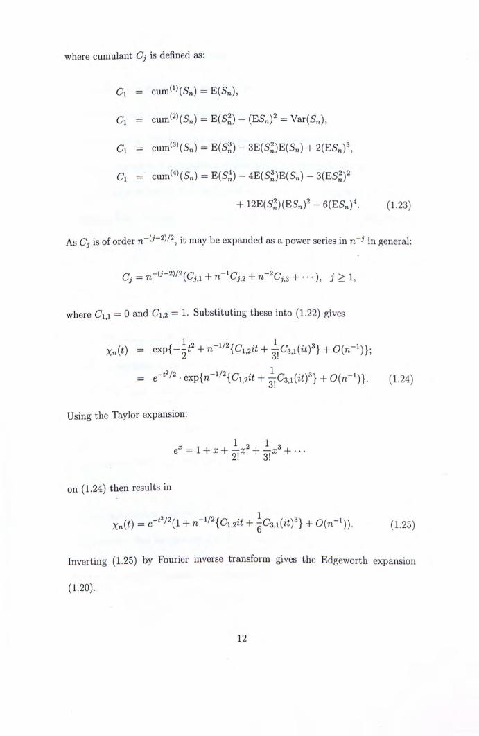
where cumulant Cj is defined as:
Ci = cum �(SVO = E(民)’
二 c u m � = 二) — =
Ci = cum � = E ( « S � - 3 E 0 S = ) E 0 S „ ) + 2(E<S„)3,
Ci = cum^'HSn) = - 4E(5^)E(5„) -
+ l2E{Sl){ESn) ' -6{ESn) ' . (1.23)
As Cj is of order ”—(••一2)/2’ it may be expanded as a power series in n—j in general:
Cj = + + + •..)’ j > h
where Ci,i = 0 and Ci,2 = 1. Substituting these into (1.22) gives
Xn(t) = exp{-^t2 + n-"2{(7i’2i< + ^3,iW3} + 0(n-i)};
= = e 部 • exp{n—i/2{Ci’2it + + O(n-i)}. (1.24)
Using the Taylor expansion:
e � 1 + + ‘ 2 + 去工3 + ….
on (1.24) then results in
X r ^ � 二 e - � 2 ( 1 + + + 0(71"^)). (1.25)
Inverting (1.25) by Fourier inverse transform gives the Edgeworth expansion
( 1 . 2 0 ) .
12
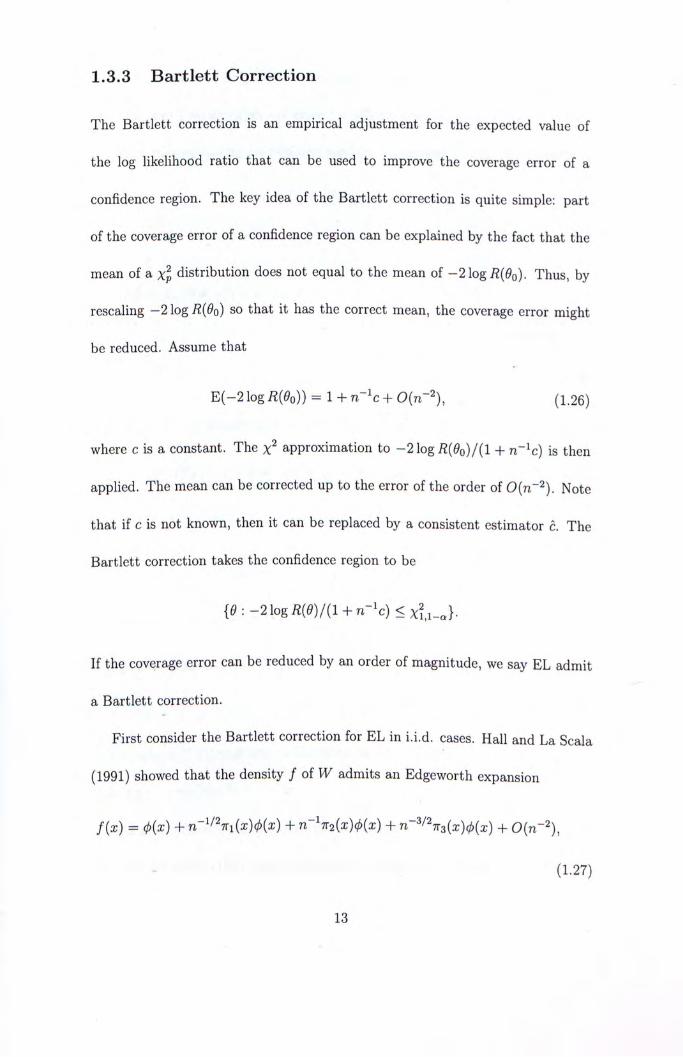
1.3.3 Bartlett Correction
The Bartlett correction is an empirical adjustment for the expected value of
the log likelihood ratio that can be used to improve the coverage error of a
confidence region. The key idea of the Bartlett correction is quite simple: part
of the coverage error of a confidence region can be explained by the fact that the
mean of a Xp distribution does not equal to the mean of —21og/?(0o). Thus, by
rescaling -21og/?(^o) so that it has the correct mean, the coverage error might
be reduced. Assume that
E ( - 2 log R{eo)) = 1 + n_ic + 0(71—2)’ (1.26)
w h e r e c is a c o n s t a n t . T h e a p p r o x i m a t i o n t o - 2 log + n ' ^ c ) is t h e n
applied. The mean can be corrected up to the error of the order of 0{n~^). Note
that if c is not known, then it can be replaced by a consistent estimator c. The
Bartlett correction takes the confidence region to be
If the coverage error can be reduced by an order of magnitude, we say EL admit
a Bartlett correction.
First consider the Bartlett correction for EL in i.i.d. cases. Hall and La Scala
(1991) showed that the density f oiW admits an Edgeworth expansion
f{x) = (f){x) + + n-'n2{x)(f)(x) + + •(n—?)’
(1.27)
13
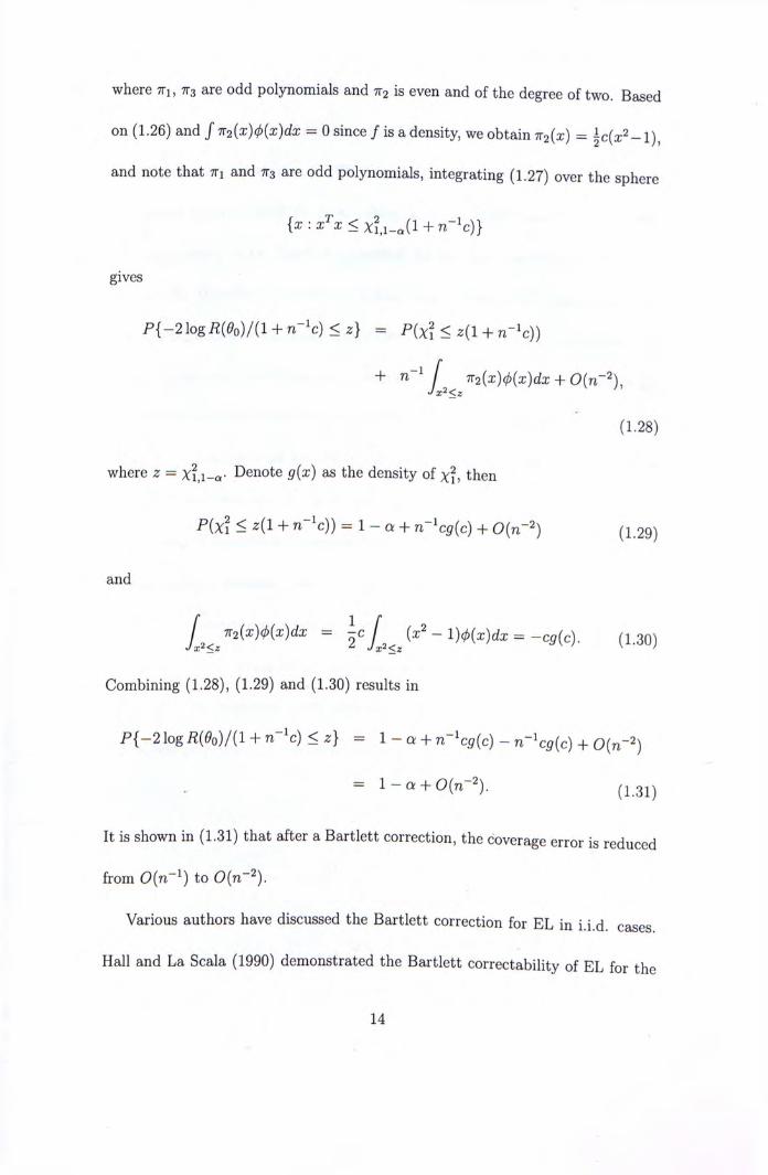
where tti, tts are odd polynomials and tt? is even and of the degree of two. Based
on (1.26) and f 7r2{x)(f){x)dx = 0 since / is a density, we obtain n2{x) = 一 i)’
and note that tti and tts are odd polynomials, integrating (1.27) over the sphere
{ 工 : +
gives
P{-2\ogR{9o)/{l + n-'c)<z} = S + n—ic))
(1 .28)
where z = x?’i_a. Denote g(x) as the density of x?’ then
P{x\ < z{l + n-^c)) = l - c v + n-^cg{c) + 0(71—2) (1.29)
and
J^^^ n2ix)(l)(x)dx = IcJ^^^ -'^)(p{x)dx =-cg{c). (1.30)
Combining (1.28), (1.29) and (1.30) results in
P{-2\ogR{9o)/il + n-'c)<z} = I - c^ + n-'cg{c) - n-'cg{c) + 0{n-')
• = 1 … 0 ( n - 2 ) . (1.31)
It is shown in (1.31) that after a Bartlett correction, the coverage error is reduced from O(n-i) to 0{n-^).
Various authors have discussed the Bartlett correction for EL in i i d cases
Hall and La Scala (1990) demonstrated the Bartlett correctability of EL for the
14
population mean, and DiCiccio, Hall, and Romano (1991) proved that EL applied
to the smooth functions of means is Bartlett correctable. Zhang (1996) showed
that the Bartlett correction for EL is applicable for 0 e R defined through the
estimation function m{X, 6) G R. Chen and Cui (2007) recently established
the applicability of the Bartlett correction for EL with over-identified moment
restrictions. However, this thesis is the first work to theoretically demonstrate the
Bartlett correction for EL in dependent cases. From the Bartlett correction for EL
in i.i.d. cases, it is known that for dependent cases the Edgeworth expansion of EL
ratio statistics must be derived first. In the following, the asymptotic expansions
of EL for dependent data are discussed, and then the Bartlett correctability of
EL in the short-memory case is demonstrated.
The rest of this thesis is organized as follows: Section 2.1 details some of the
background and necessary assumptions for the main results. Stochastic expan-
sions of EL ratio statistics are discussed in Section 2.2. Section 2.3 establishes
the validity of the formal Edgeworth expansion for the EL ratio statistic and cal-
culations of the cumulants of the statistic. The main results are given in Section
2.4. Chapter 3 provides simulation studies of the coverage error after Bartlett
correction..
15
Chapter 2
Bartlett Correction for EL
In this chapter, it is proved that EL in time series admits a Bartlett correction.
First, the EL method for time series is reviewed and the regularity conditions for
the Bartlett correction of EL presented. Stochastic expansions of the EL ratio
statistic are then explored and the Edgeworth expansion of the EL ratio statistic
is deduced. Once the cumulants of the EL ratio statistic have been calculated
and the validity of the formal Edgeworth expansion demonstrated, a closed form
of Edgeworth expansion is derived. Finally, two theorems about the Bartlett
correction of EL for time series are presented.
2.1 Empirical Likelihood in Time Series The following conditions are used in this chapter.
Assumption
16
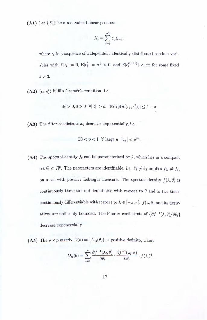
( A l ) Let {Xt} be a real-valued linear process: oo
不 = a j C t - j , j=o
where et is a sequence of independent identically distributed random vari-
ables with E[et] = 0’ E[e?] = > 0, and < oo for some fixed
s > 3.
(A2) (ei’e?) fulfills Cramer's condition, i.e.
36>0,d>0 V||t|| >d \Eexp{it'{ei,el))\ <1-6.
(A3) The filter coefficients a^ decrease exponentially, i.e.
30 < p < 1 V large u la^J < pi"!.
(A4) The spectral density fe can be parameterized by 6, which lies in a compact
set 6 C BP. The parameters are identifiable, i.e. Oi + implies fe^ + JQ^
on a set with positive Lebesgue measure. The spectral density f{X,6) is
continuously three times differentiable with respect to 6 and is two times
continuously differentiable with respect to A € [- t t , tt]. /(A, 9) and its deriv-
atives are uniformly bounded. The Fourier coefficients of 9)/d6i}
decrease exponentially.
(A5) The pxp matrix D{9) = is positive definite, where
^ d ^ ' f i ^ i ) .
17
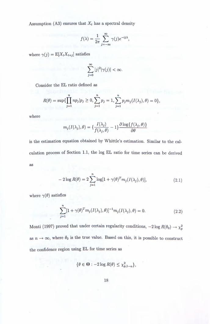
Assumption (A3) ensures that Xt has a spectral density
/ ( A ) =去 E j=—oo
where j { j ) 二 Epi^t^i^t+j] satisfies oo
E 丨 遍 ) 丨 < 沉 . 3=0
Consider the EL ratio defined as n n n
m = s u p i H ^ P i h > = = 0}, j=i j=i
where
is the estimation equation obtained by Whittle's estimation. Similar to the cal-
culation process of Section 1.1,the log EL ratio for time series can be derived
as n
一 2 log _ = 2 log[l + 7 ⑷ 了 0 ) ] ’ ( 2 . 1 )
i=i where 7(0) satisfies
n + e) = 0. (2.2)
Monti (1997) proved that under certain regularity conditions, -21og/?(0o) -> Xp
as n oo, where Gq is the true value. Based on this, it is possible to construct
the confidence region using EL for time series as
18

where xg’i_a is the 1 - a quantile of a x l distribution.
In the following sections, the coverage error of EL confidence regions for time
series is discussed and the Bartlett correctability of EL for time series is demon-
strated. As mentioned in Section 1.3, the Edgeworth expansion of the EL ratio
statistic must be obtained first.
2.2 Stochastic Expansions of EL in Time Series To derive the Edgeworth expansion of the EL ratio statistic, it is necessary to first
calculate the cumulants of the statistic. However, as the log EL ratio (2.1) con-
tains 7(0), which is not available, it is necessary to deduce a stochastic expansion
of 7(0) based on restriction (2.2).
To simplify the expansion, the following notations are defined:
� = 1 1 “
V j=l 1 “
a ( e ) 二 从 抓 • ) ’ 叫 .
V j=i Applying the Taylor expansion:
l-\-x
to restriction (2.2) gives
- r r i j i l M . X [1 - j'^rrijinXj), 6) + 約广 + ...] = 0.
19
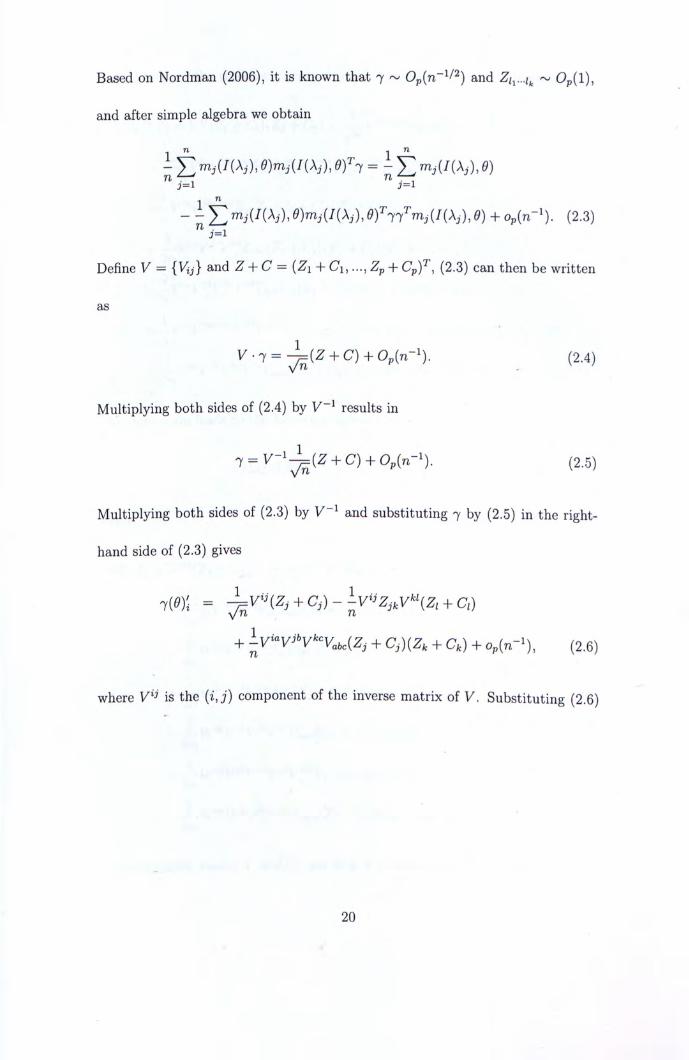
Based on Nordman (2006), it is known that 7 � O p ( n - " 2 ) and Zip..“ ~ Op(l),
and after simple algebra we obtain
- E 爪 j ( 队 e f - y mj{I{Xjl 0)
1 “ - + Op(n-^). (2.3)
Tt J=1 Define V = {Vij} and Z + C = (Zi + C i , Z p + C p f � ( 2 . 3 ) can then be written
as «
V = + + (2.4)
Multiplying both sides of (2.4) by results in
7 = + + (2.5)
Multiplying both sides of (2.3) by V ^ and substituting 7 by (2.5) in the right-
hand side of (2.3) gives
二 + c , ) - + Q)
+ + + C,) + Op(n-I), (2.6) f L
where V'^ is the { i j ) component of the inverse matrix of V. Substituting (2.6)
20
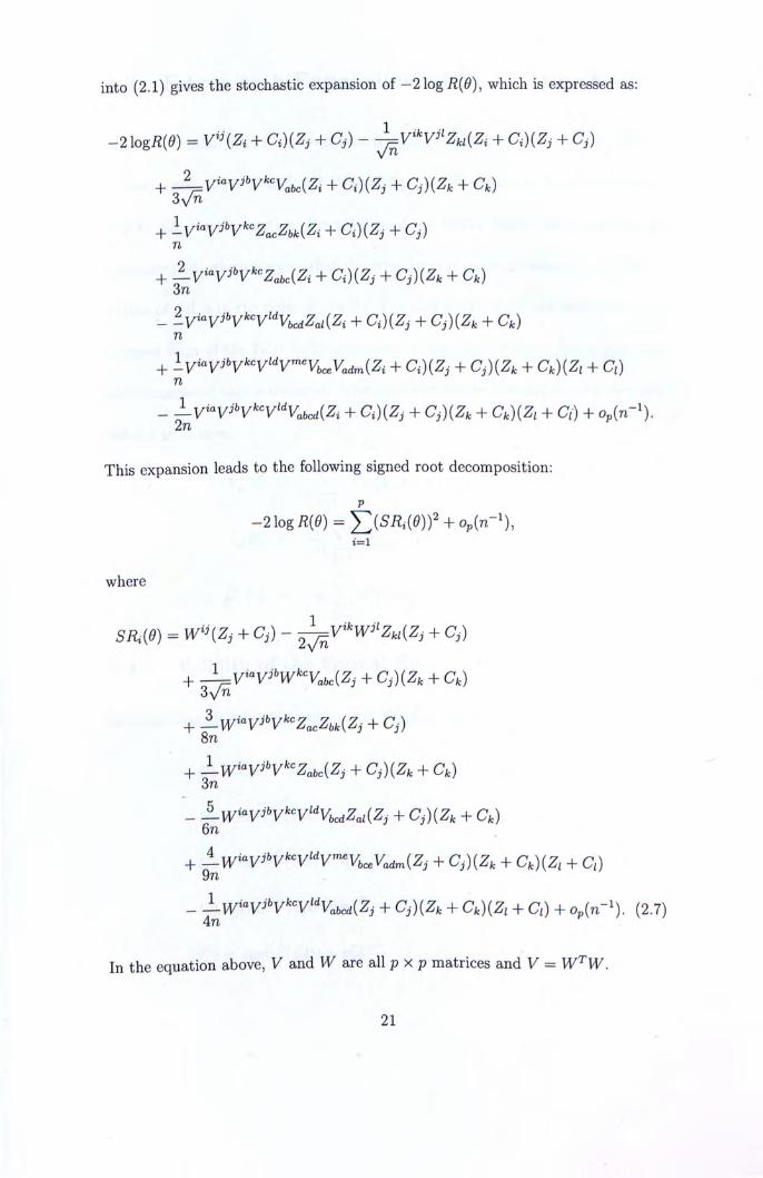
into (2.1) gives the stochastic expansion of - 2 log R{6), which is expressed as:
-2 logR(e) = + Ci){Zj + Cj) - + Ci)(Z^ + Cj)
+ + Q){Zj + + CO 3y/n + -V'^V^'V'^ZacZtkiZi + Q){Zj + Cj) n + 知 c 么“ Zi + Ci)(Zj + Cj){Zk + Ck) 3n - + C舰 + Cj){Z, + Ck) n + 〒 广 VW W Z i + Ci)(Zj + Cj)(Zk + C,){Zi + Ci) n - 丄 — • t / � � w 么 + Ci){Zj + Cj)iZ, + C,){Zi + Ci) + Op(n-I). 2n
This expansion leads to the following signed root decomposition:
i=l
where
Sim = + Ci) - + C,) + + Cj)[Z, + Ck) 3 v n + + C J ) 8n + + Cj){Z, + Ck) 3n _ + Cj)(Zk + Cfc) 6n + + + Ck){Zi + Q) 9n - + Cj){Zk + Ck){Zi + Ci) + op(n-i). (2.7) 4n
In the e q u a t i o n above, V and W are all p x p matrices and V = W'^W.
21
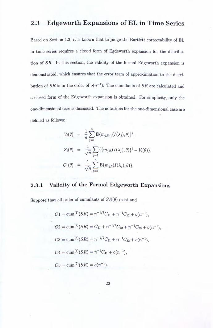
2.3 Edgeworth Expansions of EL in Time Series Based on Section 1.3, it is known that to judge the Bartlett correctability of EL
in time series requires a closed form of Egdeworth expansion for the distribu-
tion of SR. In this section, the validity of the formal Edgeworth expansion is
demonstrated, which ensures that the error term of approximation to the distri-
bution of SR is in the order of The cumulants of SR are calculated and
a closed form of the Edgeworth expansion is obtained. For simplicity, only the
one-dimensional case is discussed. The notations for the one-dimensional case are
defined as follows:
ViW =
V j=i
2.3.1 Validity of the Formal Edgeworth Expansions
Suppose that all order of cumulants of SR(9) exist and
CI = cum(i)(57?) = n 部 Cu + n-^Cn + 0(71—1),
C2 == cum(2)(57^) = C21 + n 部 Chi + n-^Css + 0(71—1)’
C3 = cum ⑶卿=71-1/2(731 + n-^C32 +
C4 = cum ⑷卿 = n - i O i i + 。 (几 ] )’
(:75 二 c u m(5)_ = 1).
22
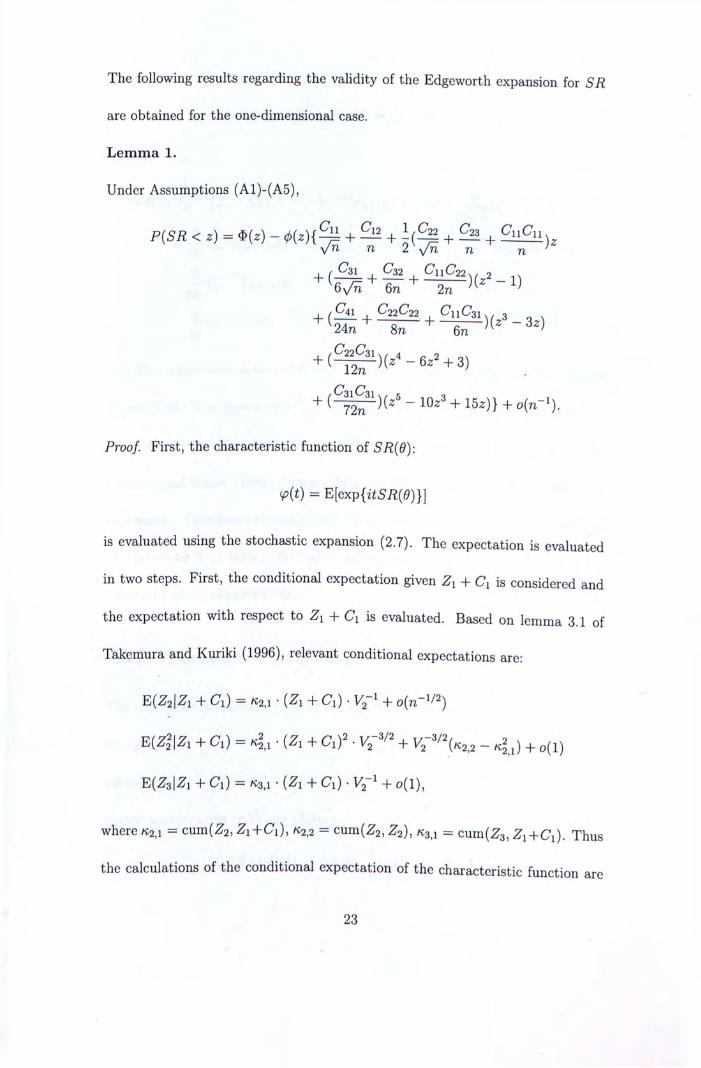
The following results regarding the validity of the Edgeworth expansion for SR
are obtained for the one-dimensional case.
Lemma 1.
Under Assumptions (A1)-(A5),
P(SR <z) = Hz) - + ^ + + ^ + Vn n n n ‘ I ( 31 C32 CuC22\, 2 IX
+ + 誓 + 孕
+ ( 發 ( 厂 6 ? + 3 ) .
+ 一 衞 3 + 1 5 … +
Proof. First, the characteristic function of SR{6):
^(t) = E[exp{itSR{e)}]
is evaluated using the stochastic expansion (2.7). The expectation is evaluated
in two steps. First, the conditional expectation given + C: is considered and
the expectation with respect to Zi + Ci is evaluated. Based on lemma 3.1 of
Takemura and Kuriki (1996), relevant conditional expectations are:
E(Z2|Zi + Ci) = «:2,1 • (Zi + C i ) . 1/2-1 + o(n-i/2)
+ Ci) = • (Zi + . ( 3 / 2 + - + o(l)
E(Z3|Zi + Ci) = K3’1 . (Zi + Ci) . 1/2-1 + 0(1),
where K2,i = cum(Z2’ ^ i+Ci ) , «;2,2 = cum(Z2, ^2), «3’1 = c u m(而’ Zi + Ci). Thus
the calculations of the conditional expectation of the characteristic function are
23
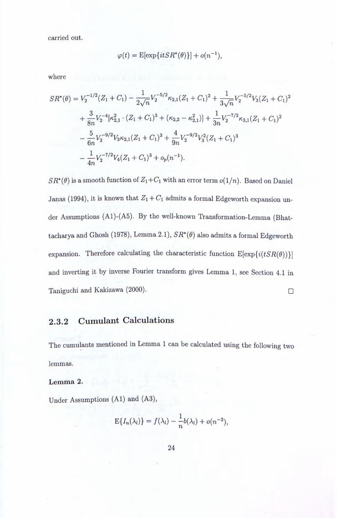
carried out. �=Elexp{itSR*{e)}] + o(n-i)’
where
SR%e) = + CO - ^ v i ' / ^ ^ A Z i + c,)' + + Ci)^
+ . + + K 2 - 4 i ) l + 去 V 7 " � i ( z i + c,)'
一^7/2柳1+。1)3 + 咖-1). 4n SR*{6) is a smooth function of Zi+Ci with an error term o(l /n) . Based on Daniel
J anas (1994), it is known that Zi + Ci admits a formal Edgeworth expansion un-
der Assumptions (A1)-(A5). By the well-known Transformation-Lemma (Bhat-
tacharya and Ghosh (1978), Lemma 2.1), SR*(e) also admits a formal Edgeworth
expansion.
Therefore calculating the characteristic function E[exp{i{tSR{9))}]
and inverting it by inverse Fourier transform gives Lemma 1’ see Section 4.1 in
Taniguchi and Kakizawa (2000). 口 2.3.2 Cumulant Calculations
The cumulants mentioned in Lemma 1 can be calculated using the following two
lemmas.
Lemma 2.
Under Assumptions (Al) and (A3),
E{IniXi)} = f{Xi)-h{Xi) + o{n-^), 71/
24
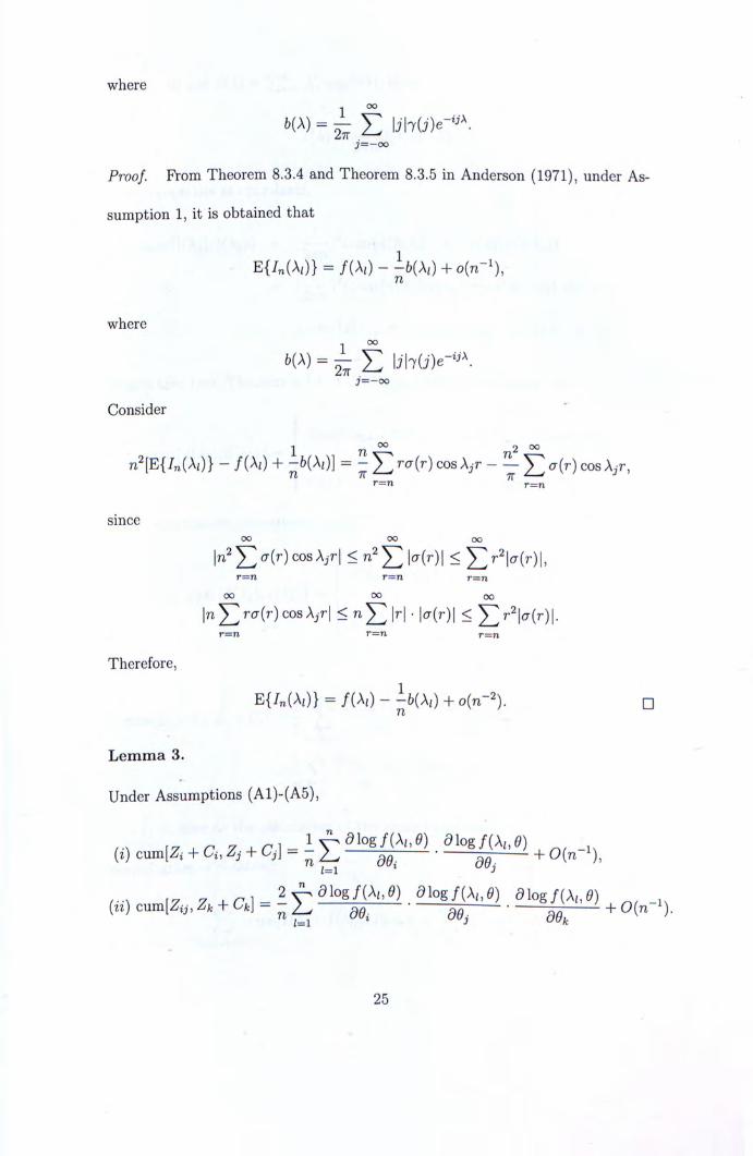
where 1 °°
bW = ^ E b•丨7We-, j = - o o
Proof. From Theorem 8.3.4 and Theorem 8.3.5 in Anderson (1971),under As-sumption 1, it is obtained that
n
where 1 °°
bW = ^ E b . l 7 � e -j=—oo
Consider “
1 Tl ^ 2 � n'[E{In{Xi)} 一 /(AO + -b{Xi)] = Mr) cos V — ^ E cos V ’
71 TT 71" ' “ r=Ti r = n since
oo oo oo |n2 [ • ) cos A , | S n2 ;^ |a(r) | < £ r ' \ a { r ) l
r=n r=n r—n oo oo oo
| n 5 > a ( r ) c o s A , | S |r| . |a(r) | < 5 > 2 | a ( r ) | . r=n r=n r = n
Therefore, E{In{Xi)} = f{Xi)-h{Xi) + o{n-'). •
71/ Lemma 3.
Under Assumptions (A1)-(A5),
� c — z , + a , z , + c , 二 1 E ^ ^ ^ . ^ ^ +
, . . � f 7 r 4 r 1 2 f ^ a i o g / ( A , ’約 d\ogf{\,,e) a log/(A, ’ 的 … ,
25
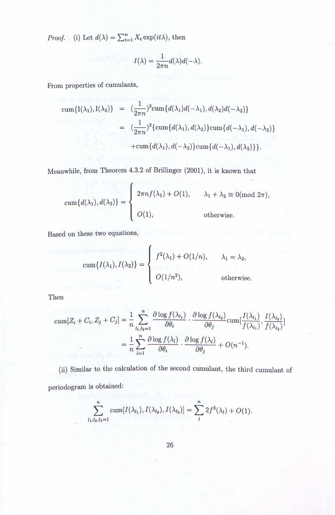
Proof, (i) Let d{X) = ^t exp(itA), then
/(A) = ^ d { X ) d { - X ) .
From properties of cumulants,
cum{I(Ai),I(A2)} = (^)^cum{d(Ai)d(-Ai) ,d(A2)d(-A2)}
= ( i ) 2 { c u m { d ( A i ) , d(A2)}cum{d(-Ai), d(-入 2)} znn
+cum{d(Ai), d(-A2)}cum{d(-Ai), d{\2)}}.
Meanwhile, from Theorem 4.3.2 of Brillinger (2001), it is known that
2nnf (入 1) + 0(1), 入1 + 入2 三 O(mod 27r), cum{d(Ai),d(A2)}= < 0(1), otherwise.
� Based on these two equations,
/2(Ai) + 0 ( l / n ) , Ai = A2, cum{/(Ai),/(A2)}= <
0 ( l /n^ ) , otherwise. �
Then
口 … 1 ^ log/(A/J a l o g / � J { K ) / � 1 cum[么 + C“ Z, + C , ] = - E 飞 — ]
i ^ a i o g / ( A O a l o g / � , � £ = 1 •‘
(ii) Similar to the calculation of the second cumulant, the third cumulant of
periodogram is obtained: 亡 cum[ / (Aj , / (A^J , / ( � ) ] = ^ 2 f ( A 0 + 0(1).
il’W3 = l ‘
26
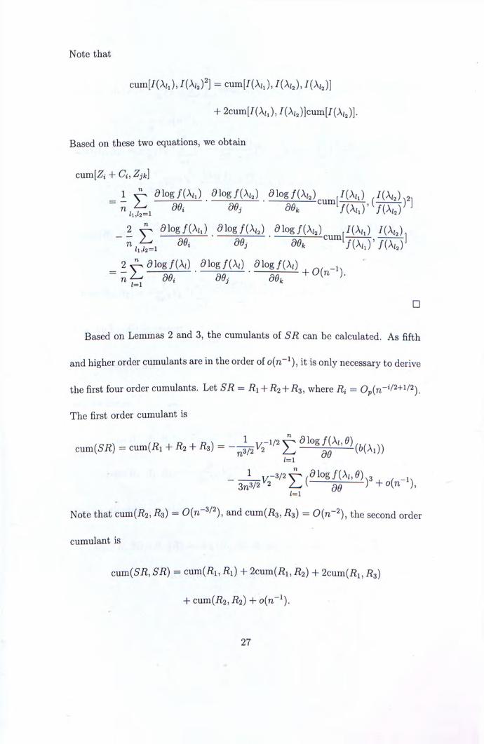
Note that
+ 2 c u m [ / ( A i J , / ( A i J ] c u m [ / ( A i J ] .
Based on these two equations, we obtain
cum[Zi + Ci, Zjk] 二 1 亡 ^ log / (A, ) . ^ log / (A , ) / (A,) / ( A �
_ 2 y - … o g / ( A“) a log/(A,2) a log/(A,2) f / � I{X.)
_ 2 ^ a i o g / ( A , ) a l o g / � <9 log/(AO 1 • ~ n ^ de, + ).
•
Based on Lemmas 2 and 3, the cumulants of SR can be calculated. As fifth
and higher order cumulants are in the order of it is only necessary to derive
the first four order cumulants. Let SR = + where Ri = Op(n-"2+i/2)
The first order cumulant is
c u m 卿 = + + i^s) = - ‘ 1 ^ / 2 亡 1=1 OU
- v - 3 / 2 .^log /(Ai, 6) 3n3/2 h L ( QQ )3 + o(n-i), /=1 Note that cum(/?2, Rz) = 0(n-3/2)’ and cum(i?3, Rz) = 0(n-2), the second order
cumulant is
cnm{SR, SR) = cum(Ri,Ri) + 2cum(i?i’ + 2cum(i?i, i^g)
+ cum(i?2’ 丑 2) + o(n""i).
27
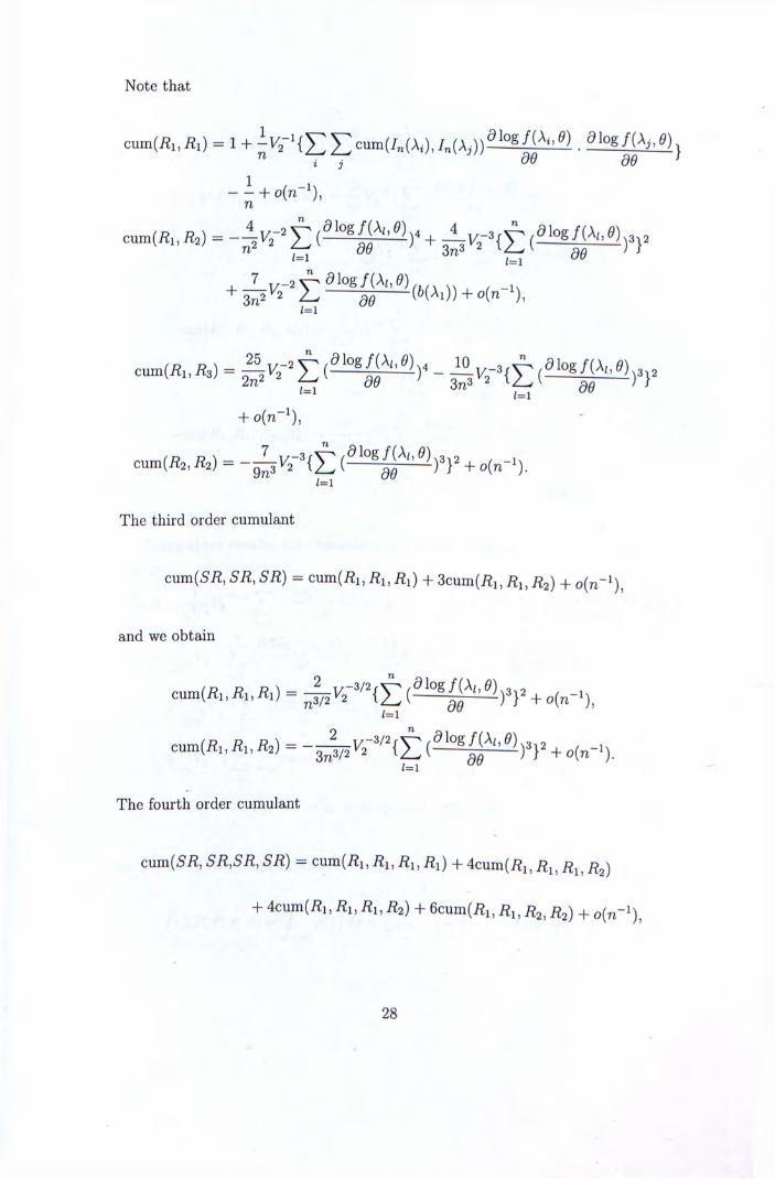
Note that
cum(/?i’/?i) = 1 + ^Vi'iY: E 4(A,)) ^ I M . ^ i M x 几 i i do de !
-1),
c 一 1 ’ = — > 2-2 E + ( ^ 1 ^ ) 3 ) 2
1=1
C一 l ’ i ^ 3 ) 二 — S u e /=1
+ o(n-”’ •
cum(i^2’ = - ^ V f ^ f E i'-^^^rr + � ( n - i ) . 1=1
The third order cumulant
cum{SR, SR, SR) = cum(i?i, R^, R^) + 3cum(i?i, i^i, R2) +
and we obtain
_ ( 凡 ’ 历 ’ 凡 ) = + + 一 1),
The fourth order cumulant
cum(S7?’ SR,SR, SR) 二 cum(/?i, RuRi,Ri) + 4cum(/?i’ i?�’ j^i,
+ icum{RuRu Ru R2) + 6 c u m ( / ? i , R 2 ) + o(n—
28
and
cum(瓜,Ri, R u R . ) = > 2 - 2 E 严 + 。 ( 几 - 1 ) ,
孔 1=1 o" cuHRuRuRuR.) = 严
1=1
1=1
+ ~ ^ ~ ) + + ). 1=1
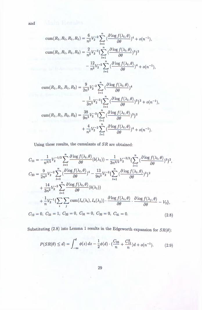
Using these results, the cumulants of SR are obtained:
Cu - E ^ 圖 - ‘ 們 : f : ( ^ ^ m "‘ 1=1 i=i ^ 9 1广 2 .dlog f{Xi,e), 一 3 r V . S O o g / ^ C23 二 乙 L -QQ ) ^ ))
1 = 1 Z = 1
^ i j
C12 二 0’ C21 = 1, C22 = 0, Cai = 0, C32 = 0, C41 = 0. (2.8)
Substituting (2.8) into Lemma 1 results in the Edgeworth expansion for SR(0}:
P(SR(0} <d)= f (p{z) dz - \ m . + 还)d + o(n-i). (2.9) J-00 ^ 71
29

2.4 Main Results Based on the validity of the formal Edgeworth expansion and cumulant calcula-tions, a theorem about the coverage error of the EL confidence region for time series can be elaborated. Theorem 1. If Assumptions (Al)-(A5) hold, then
P{-2 log R{9) <dc^) = l - a + O(n-i)’
where da from a Xi table such that
P { x l <dc,) = l - a . .. (2.10)
Proof. Since the distribution function of SR{e) admits an Edgeworth expansion
(2.9), then
P{-2\ogR{e)<da) = P(SR(0)2 s d。)+ o(n-i)
= H z ) + o(n-') J-孤 n n ^ ‘
= l _ a + 0(n-i). •
Theorem 1 indicates that the EL confidence region for time series models has
a coverage error of the order of The Bartlett correction can be applied
to improve the accuracy of the chi-squared approximation from order to
order Based on the cumulants of SR{B), it can be shown that
E[-2\og R(9)] = E[SR{ef + o(n-i)] = � ]
+ (cum � [ 5 7 ? � ] +
= 1 +三+ o(n-i)’ n
30

where
c = C23 + Cfi’ (2.11) C23 and Cii are given in (2.8). Theorem 2. If Assumptions (Al)-(A5) hold, then
P(-2logR{0) < cUl + c/n)) = 1 — a + 0(71"^),
where c is the Bartlett correction factor given by (2.11), d^ is defined in (2.10).
Proof. Applying the Edgeworth expansion (2.9) results in
P(-21og_ < dM + = P(SR(Of < dM + -)) + • - ” Th
=Pixl < da(l + - + + o(n-i)
= + n-icx/^(27r 广 1 � - ‘ / 2 一 + o[n-')
= 1 - a + o(n~^). 口
Theorem 2 establishes that the Bartlett correction reduced the coverage error
from O(n-i) to o(n-^). However, as the true value of c is not known in practice,
it should be estimated from the sample which is discussed in the next
chapter.
31
Chapter 3
Simulations
In this chapter, several Monte Carlo experiments are performed to demonstrate
the Bartlett correctability of EL for time series models. A simple ARMA(1,1)
model is used in the experiments. All programs are written in MATLAB
The ARMA(1,1) process Xt with the parameter 6 and 0 can be expressed as:
Xt = (f>Xt-i + Zt- eZt-u Zt �WN(0,CT2)’ (3 1)
where cr is assumed to be known.
In the ARMA(1,1) model simulation, Xt is simulated iteratively with equation
(3.1) for t 二 1,."’3T. This series is then selected from 2T + 1 to 3T as the
ARMA(1,1) model for the experiments.
32
3.1 Confidence Region Recall from Monti (1997) that the EL ratio statistic - 2 log R{e) is asymptotically
distributed as Xp, where 6 belongs to the parameter space 0 with a dimension
p. Consequently, an approximate 1 - a confidence region with an asymptotic
coverage level a is given by
where Xp,i-a is the 1 - o; quantile of a Xp distribution. In practice, the confidence
region is constructed by calculating - 2 log R{9) at different mesh points over the
parameter space and comparing the results with the threshold value Xp i-a
Estimation of Bartlett Correction Factor To obtain the confidence region after the Bartlett correction, it is necessary to
estimate the value of the Bartlett correction factor c from the sample X i , . . . ,
Similar to the bootstrap method for time series models mentioned by Monti
(1997),c is estimated as the following procedure. Let
where On is the consistent estimator of 9. Let F^ be the empirical distribution
function that attaches mass to each yj. A bootstrap sample -^yn)
can be obtained by resampling from Fn with replacement (see Franke and Hardle,
1992). A sample of periodogram ordinates
/ � A i ) ’ , ( A 2 ) ’ . " ’ / U 0 ’
33
can then be obtained, where for each j,
, ⑷ = / ( A 力 叫
Each set of {/^(Ai),广(A2)’ …’广(\z)} provides a replication - 2 log R\9r,) of
-2\og R{6) at On- The resampling method is repeated B times and the Bartlett
correction is then
1 B 1 + (3.2) 6 = 1
From (3.2) the value of c can be estimated. Consequently, the confidence region
is corrected as:
71/
Example 1 In this example, the construction of confidence regions is demonstrated and
the EL confidence regions and Bartlett corrected EL confidence regions are com-
pared.
Consider the ARMA(1,1) case with ^ = 0.8 , 0 = 0.2 and a series length
T = 1000. Zt is standard normal. An ARMA(1’1) series { X J is simulated and
-2\og R(9) is calculated at different points over the parameter space (0,0) e
{[0,1] X [0,0.5]} to produce a contour plot using the threshold value x!’o.95 for
the construction of a 95% confidence region.
For the Bartlett corrected confidence region, c is estimated from the sample
series Xt by using equation (3.2) with B = 500 iterations in the resampling
34
procedure of the Bartlett correction. Another contour plot is then produced
using the threshold value xlo.95(l + c) to construct the 95% confidence region.
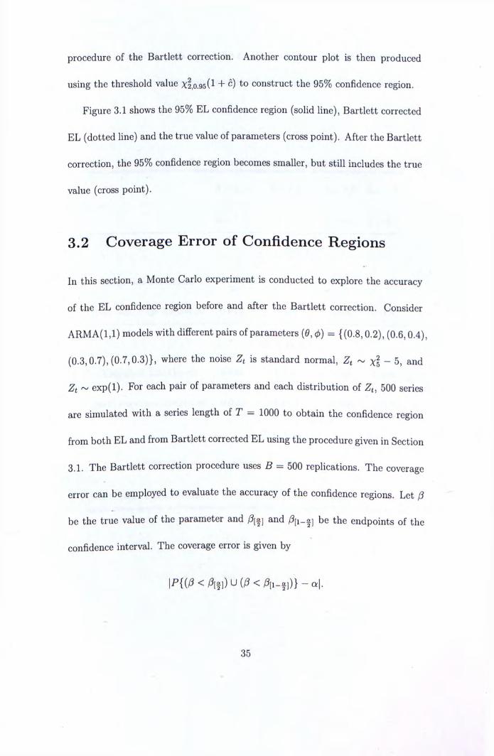
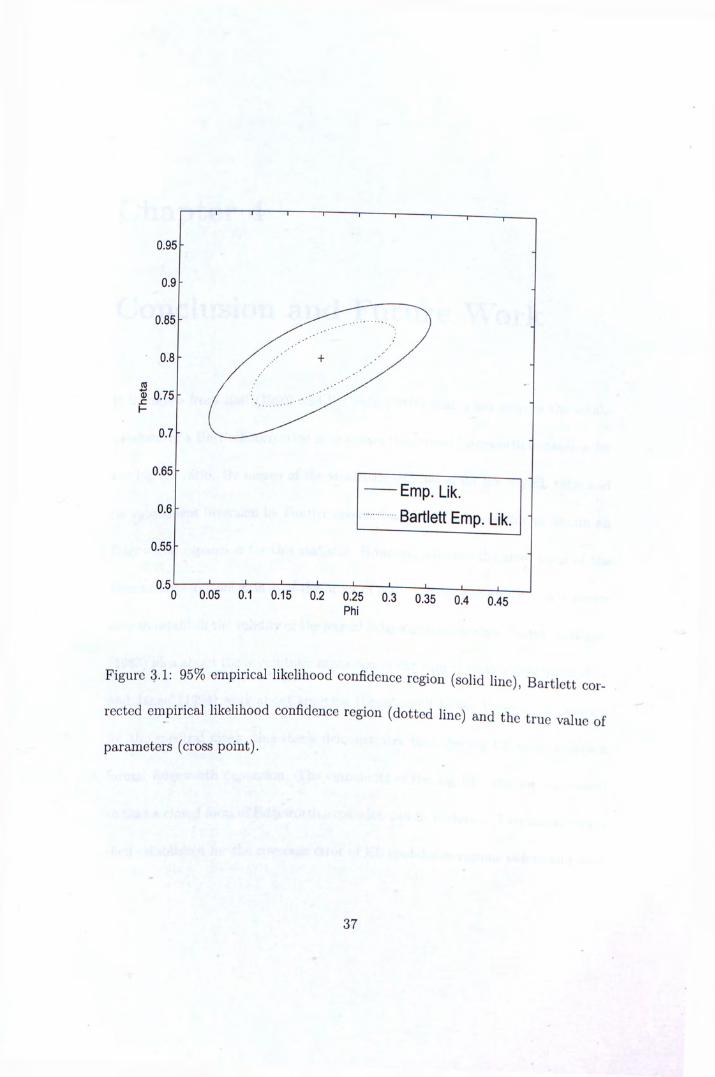
Figure 3.1 shows the 95% EL confidence region (solid line), Bartlett correctcd
EL (dotted line) and the true value of parameters (cross point). After the Bartlett
co r r ec t i on , the 95% confidence region becomes smaller, but still includes the true
value (cross point).
3.2 Coverage Error of Confidence Regions In this section, a Monte Carlo experiment is conducted to explore the accuracy
of the EL confidence region before and after the Bartlett correction. Consider
ARMA(1’1) models with different pairs of parameters (0’ 0) = {(0.8,0.2), (0.6’ 0.4),
(0.3’ 0.7), (0.7’ 0.3)}’ where the noise Zt is standard normal, Zt � x ! - 5, and
Zt � e x p ( l ) . For each pair of parameters and each distribution of Z^ 500 series
are simulated with a series length of T = 1000 to obtain the confidence region
from both EL and from Bartlett corrected EL using the procedure given in Section
3.1. The Bartlett correction procedure uses B = 500 replications. The coverage
error can be employed to evaluate the accuracy of the confidence regions. Let (3
be the true value of the parameter and [晉]and be the endpoints of the
confidence interval. The coverage error is given by
35

Table 3.1 shows the results when the confidence level is 0.95 and illustrated the
Bartlett correction successfully reduces the coverage error of EL confidence re-
gions.
Table 3.1: Coverage errors of confidence regions for ARM A (1,1) models
“0.8 ^ = 0.6 e = 0.7 9 = 0.3
0 = 0.2 0 = 0.4 0 = 0.3 0 = 0.7
Zt � i V ( 0 , 1 )
Empirical Likelihood 0.048 0.046 0.048 0 048
Bart, crnpirical likelihood 0.018 0.004 0.006 0 008
Zt � X s — 5
Empirical Likelihood 0.048 0.046 0.046 0.044
Bart, empirical likelihood 0.020 0.016 0.000 0 008
Z j t � e x p �
Empirical Likelihood 0.040 0.050 0.042 0.046
Bart, empirical likelihood 0.006 0.020 0.000 • 000
36
r 1 I I -r 1 -I 1 -1 0.95 - -
0.9 • -
I 0.75- / : . � . . . . … ^ ^ ^ ^ -0.7 - V _ _ _ .
0.65 Emp. Lik.
0.6 • Bartlett Emp. L i k . " 0.55 - -
0.51 ‘ ‘ ‘ ‘ ‘ 1 1 — — - i 1 0 0.05 0.1 0.15 0.2 0.25 0.3 0.35 0.4 0 45
Phi
Figure 3.1: 95% empirical likelihood corifidencc region (solid line), Bartlett cor-rected empirical likelihood confidencc region (dotted line) and the true value of parameters (cross point).
37
Chapter 4
Conclusion and Future Work
It is known from Hall (1990) and DiCiccio (1991) that a key step in the estab-
lishment of a Bartlett correction is to obtain the formal Edgeworth expansion for
the log EL ratio. By means of the stochastic expansion for the log EL ratio and
its subsequent inversion by Fourier inverse transform, it is possible to obtain an
Edgeworth expansion for this statistic. However, whether the error term of the
Fourier inverse transform is of the order of is not known, then it is neces-
sary to establish the validity of the formal Edgeworth expansion. Based on Hipps'
(1983) idea about the asymptotic expansion of the sum of weakly dependent data
and Janas' (1994) work about applying Hipps,result to the Whittle's estimation
for the spectral mean, this thesis demonstrates that the log EL ratio admits a
formal Edgeworth expansion. The cumulants of the log EL ratio are calculated
so that a closed form of Edgeworth expansion can be deduced. Two theorems are
then established for the coverage error of EL confidence regions before and after
38
Bartlett correction, which comprise the main results of this thesis.
Finite sample simulations are conducted and the construction of confidence
regions using the log EL ratio is demonstrated. A bootstrap procedure is pro-
posed to obtain the Bartlett correction factor for the statistic and a Monto Carlo
simulation is conducted to explore the coverage error of EL confidence regions be-
fore and after Bartlett correction. It is shown that the Bartlett correction greatly
reduces the coverage error of EL confidence regions.
The results are obtained only for the short-memory and one-dimensional cases
and the stochastic expansion of —2 log R{6) is deduced for p-dimensional cases.
‘ F u t u r e work could extend the results to p-dimensional cases by obtaining the
Edgeworth expansion for p-dimensional cases. Although the validity of the formal
Edgeworth expansion can be proved in a manner similar to that used for the one-
dimensional case, the calculations of cumulants are likely to be formidable.
The extension of this work to the long-memory case is likely to be much more
difficult to pursue than the extension to p-dimensional cases. Although simulation
results suggest that EL for the long-memory case is Bartlett correctable, especially
when a is small, this still needs to be established theoretically. A particular
d i f f i cu l ty .wi th this will be demonstrating the validity of the formal Edgeworth
expans ion . To the best of the author's knowledge, there are few papers that
discuss the Edgeworth expansion for long-range dependent data. Determining the
orders of the cumulants is also likely to be difficult. For example, the expected
periodogram in the short-memory case has an asymptotic expansion, and it is
39
known that its order decay to zero. Unfortunately, the corresponding order in
the long-memory case is not known, and requires exploration in the future.
To conclude, this thesis establishes the validity of the formal Edgeworth ex-
pansion for the log EL ratio in the short-memory case. After onerous calculation,
the cumulants and a closed form of Edgeworth expansion for this statistic are
obtained. It is demonstrated that the coverage error in the chi-square approx-
imation to the distribution of the log EL ratio is of the order of 0(n"^). It
is then shown that the coverage error can be reduced to o(n—i) by applying a
Bartlett correction. The Bartlett correction of EL for the short-memory case is
also illustrated in a simulation study.
40
Bibliography
[1] Anderson, T.W. (1971). The Statistical Analysis of Time Series. New York:
John Wiley & Sons.
[2] Bhattacharya, R.N. and Ghosh, J.K. (1978). On the validity of the formal
Edgeworth expansion. Ann. Statist. 6,434—451.
[3] Brillinger, D.R. (2001). Time series: Data Analysis and Theory, 2nd Ed.
San Francisco : Holden-Day.
[4] Chan, N.H. (2002). Time series: Application to Finance. New York: John
Wiley k Sons.
[5] Chen, S.X. and Cui, H. (2007). On the second properties of empirical likeli-
hood with moment restrictions. Journal of Econometrics 141, 492-516.
[6] Cramer, H. (1928). On the composition of elementary errors. Skand. Aktua-
rietidskr. 11, 13-74, 141-180.
[7] Diciccio, T.’ Hall, P. and Romano,J. (1991). Empirical likelihood is Bartlett-
correctable. Ann. Statist 19, 1053-1061.
41
[8] Franke, J. and Hardle, W. (1992). On boostrapping kernal spectral estimates.
Ann. Statist. 20, 121-145.
[9] Gotze, F. and Hipp, C. (1983). Asymptotic expansions for sums of weakly
dependent random vectors. Probability Theory and Related Fields 64, 211-
239.
[10] Hall, P. and La Scala, B. (1990). Methodology and algorithms of empirical
likelihood. Intemat. Statist. Rev. 58, 109-127.
[11] Hall, P. (1992). The Bootstrap and Edgeworth Expansion. New York
:Springer-Verlag.
[12] J anas, D. (1994). Edgeworth expansion for spectral mean estimates with
application to whittle estimates . Ann. Inst. Statist. Math. 46, 667-682.
|13j Kitamura, Y. (1997). Empirical likelihood methods with weakly dependent
processes. Ann. Statist. 25, 2084-2102.
[14] Monti, A.C. (1997). Empirical likelihood confidence regions in time series
models. Biometrika 84,395-405.
[15] Nordman, D.J. and Lahiri, S.N. (2006). A frequency domain empirical like-
lihood for short- and long-range dependence. Ann. Statist. 34, 3019-3050.
42

[16] Nordman, D.J. , Sibbertsen, P. and Lahiri, S.N. (2007). Empirical likeli-
hood confidence intervals for the mean of a long-range dependent processes.
Journal of Time Series Analysis 28, 576-599.
[17] Owen, A.B. (1988). Empirical likelihood ratio confidence intervals for a single
functional. Biometrika 75, 237-249.
[18] Owen, A.B. (1990). Empirical likelihood ratio confidence regions. Ann. Sta-
tist. 18, 90-120.
[19] Owen, A.B. (2001). Empirical Likelihood. New York: Chapman k Hall .
[20] Qin, J. and Lawless, J. (1994). Empirical likelihood and general estimating
equations. Ann. Statist. 22, 300-325.
[21] Takemura, A. and Kuriki, S. (1996). A proof of independent bartlett cor-
rectability of nested likelihood ratio tests. Ann. Inst. Statist. Math. 48’ 603-
620.
[22] Tamaki, K. (2008). Power properties of empirical likelihood for stationary
processes. Technical report, Waseda University.
[23] Tanikuchi, M. and Kakizawa, Y. (2000). Asymptotic Theory of Statistical
Inference for Time Series. New York :Springer-Verlag.
[24] Whittle, P. (1953). Estimation and information in stationary time series.
Archiv. Math. 2, 423-434.
43
[25] Zhang, B. (1996). On the accuracy of empirical likelihood confidence intervals
for M-Funtionals. Journal of Nonparametric Statistics 6’ 311-321.
44


C U H K L i b r a r i e s
0 0 4 6 5 9 8 5 5