Asymptotic spreading for generalheterogeneous Fisher-KPP type equations

Henri Berestycki a and Gregoire Nadin b

a Ecole des Hautes en Sciences Sociales, PSL research university, CNRS,

CAMS, 190-198 avenue de France, F-75013 Paris, France

b CNRS, UMR 7598, Laboratoire Jacques-Louis Lions, F-75005 Paris, France

February 10, 2016

Abstract

In this article, we establish spreading properties for heterogeneous Fisher-KPPreaction-diffusion equations:

∂tu−N∑

i,j=1

ai,j(t, x)∂iju−N∑i=1

qi(t, x)∂iu = f(t, x, u), (1)

for initial data with compact support, where the nonlinearity f admits 0 as an unstablesteady state and 1 as a globally attractive one. Here, the coefficients ai,j , qi, f are onlyassumed to be uniformly elliptic, continuous and bounded in (t, x). We constructtwo non-empty star-shaped compact sets S ⊂ S ⊂ RN such that for all compact setK ⊂ int(S) (resp. all closed set F ⊂ RN\S), one has limt→+∞ supx∈tK |u(t, x)− 1| = 0(resp. limt→+∞ supx∈tF |u(t, x)| = 0).

The characterization of these sets involve two new notions of generalized principaleigenvalues for linear parabolic operators in unbounded domains. It gives in particularan exact asymptotic speed of propagation for almost periodic, asymptotically almostperiodic, uniquely ergodic and radially periodic equations (where S = S) and explicitbounds on the location of the transition between 0 and 1 in spatially homogeneousequations. In dimension N , if the coefficients converge in radial segments, then S = Sand this set is characterized using some geometric optics minimization problem, whichmay give rise to non-convex expansion sets.

Key-words: Propagation and spreading properties, Heterogeneous reaction-diffusion equa-tions, Principal eigenvalues, Linear parabolic operator, Hamilton-Jacobi equations, Homog-enization, Almost periodicity, Unique ergodicity.

AMS classification. Primary: 35B40, 35B27, 35K57. Secondary: 35B50, 35K10, 35P05,47B65, 49L25.

1

The research leading to these results has received funding from the European ResearchCouncil under the European Union’s Seventh Framework Programme (FP/2007-2013) /ERC Grant Agreement n.321186 - ReaDi -Reaction-Diffusion Equations, Propagation andModelling held by Henri Berestycki.

1 Introduction and statement of the results

This paper is devoted to the large time behaviour of the solutions of the Cauchy problem:∂tu−

∑Ni,j=1 ai,j(t, x)∂iju−

∑Ni=1 qi(t, x)∂iu = f(t, x, u) in (0,∞)× RN ,

u(0, x) = u0(x) for all x ∈ RN .(2)

where the coefficients (ai,j)i,j, (qi)i and f are only assumed to be uniformly continuous,bounded in (t, x) and the matrix field (ai,j)i,j is uniformly elliptic. In the sequel we will often

use the Einstein convention: the sums∑N

i,j=1 and∑N

i=1 will be implicit. The reaction termf is supposed to be monostable and of KPP type, meaning that it admits two steady states0 and 1, 0 being unstable and 1 being globally attractive, and that it is below its tangent atthe unstable steady state 0. This will be made more precise later in a general framework.A typical example of such nonlinearity is f(t, x, s) = b(t, x)s(1 − s) with b bounded andinfR×RN b > 0. Lastly, we consider compactly supported initial data u0 with 0 ≤ u0 ≤ 1.

This equation arises in many contexts of biology, physics and population ecology (forthe original motivation in population genetics, see [4, 30, 44]). The goal of this paper is tostudy spreading properties for this problem. That is, we want to characterize two non-emptycompact sets S ⊂ S ⊂ RN as sharply as possible so that

for all compact set K ⊂ intS, limt→+∞

supx∈tK |u(t, x)− 1|

= 0,for all closed set F ⊂ RN\S, limt→+∞

supx∈tF |u(t, x)|

= 0.

(3)

1.1 Setting of the problem

The main purpose of the present paper is to prove spreading properties in general hetero-geneous media. Heterogeneity can arise for different reasons, owing to the geometry or tothe coefficients in the equation. Regarding geometry, the first author together with Hameland Nadirashvili [15] have studied spreading properties for the homogeneous equation ingeneral unbounded domains (these include spirals, complementaries of infinite combs, cusps,etc.) with Neumann boundary conditions. In these geometries, linear spreading speeds donot always exist. Furthermore, several examples are constructed in [15] where the spreadingspeed is either infinite or null.

The present paper deals with heterogeneous media for problems set in RN but in whichthe terms in the equation are allowed to depend on space and time in a fairly general fashion.As in [15], given any compactly supported initial datum u0 and the corresponding solution

2

u of (2), we introduce two speeds:

w∗(e) := sup w ≥ 0, for all w′ ∈ [0, w], limt→+∞ u(t, x+ w′te) = 1 loc. x ∈ RN,

w∗(e) := inf w ≥ 0, for all w′ ≥ w, limt→+∞ u(t, x+ w′te) = 0 loc. x ∈ RN.(4)

We could reformulate the goal of this paper in the following way: we want to get accurate es-timates on w∗(e) and w∗(e) and to try to identify classes of equations for which w∗(e) = w∗(e)(and is independent of u0). This last equality does not always hold, which justifies the in-troduction of two speeds rather than a single one. Indeed, Garnier, Giletti and the secondauthor [35] exhibited an example of space heterogeneous equation in dimension 1 for whichthere exists a range of speeds w such that the ω−limit set of t 7→ u(t, wt) is [0, 1]. In thiscase the location of the transition between 0 and 1 oscillates within the interval (w∗t, w

∗t)at large time t.

Together with Hamel, the authors have proved in a previous paper [12] that under anatural positivity assumption, but otherwise in a general framework, there is at least apositive linear spreading speed, which means with the above definition that w∗(e) > 0for any e ∈ SN−1. More precisely, we proved1 in [12] that if q(t, x) = ∇ · A(t, x), whereA(t, x) =

(ai,j(t, x)

)i,j

(hence we assume a divergence form operator), and f ′u(t, x, 0) > 0

uniformly when |x| is large, the following inequality holds:

w∗(e) ≥ w0 := 2√

lim inf|x|→+∞

inft∈R+

γ(t, x)f ′u(t, x, 0), (5)

where γ(t, x) is the smallest eigenvalue of the matrix A(t, x). We also established upperestimates on w∗(e), which ensure that supe∈SN−1 w∗(e) < +∞, under mild hypotheses on A,q and f .

We point out a corollary of this result. Assume that q ≡ 0 and

f(t, x, s) = (b0 − b(x))s(1− s)

with b0 > 0, b ≥ 0 and b = b(x) as well as A(x) − IN are smooth compactly supportedperturbations of the homogeneous equation. Then the result of [12] gives w∗(e) ≥ w0 = 2

√b0.

It is also easy to check that w∗(e) ≤ 2√b0 since f(t, x, s) ≤ b0s(1− s). Thus, in this case

w∗(e) = w∗(e) = 2√b0.

This result was also derived by Kong and Shen in [45], who considered other types of dis-persion rules as well. This simple observation shows that, in a sense, only what happens atinfinity plays a role in the computation of w∗(e) and w∗(e).

On the other hand, when the coefficients are space-time periodic, the expansion set couldbe characterized through periodic principal eigenvalues [12, 33, 81]. We will recall theseresults in details in Section 3.2 below and show that it could be recovered as corollaries of

1Actually, the result we obtained in [12] is a little more accurate and the hypotheses are somewhat moregeneral, we refer the reader to [12] for the precise assumptions.

3

our main result. In this framework, estimate (5) is not optimal in general: one needs to takeinto account the whole structure of equation (2) through the periodic principal eigenvaluesof the linearized equation in the neighbourhood of u = 0 to get an accurate result.

Summarizing the indications from periodic and compactly supported heterogeneities, toestimate w∗(e) and w∗(e), we see that we need to take into account:

• the behaviour of the operator when |t| → +∞ and |x| → +∞, and

• some notion of “principal eigenvalue” of the linearized parabolic operator near u = 0.

Therefore, we are led to extend the notion of principal eigenvalues to linear parabolicoperators in unbounded domains. We will define these generalized principal eigenvaluesthrough the existence of sub or supersolutions of the linear equation (see the definitionsin Section 1.3 below). This definition is similar, but different from, the definition of thegeneralized principal eigenvalue of an elliptic operator introduced by Berestycki, Nirenbergand Varadhan [19] for bounded domains and extended to unbounded ones by Berestycki,Hamel and Rossi [17]. Some important properties of classical principal eigenvalues are notsatisfied by generalized principal eigenvalues and thus the classical techniques that havebeen used to prove spreading properties in periodic media in [12, 32, 33, 81] are no longeravailable here. This is why we use homogenization techniques. In Section 5, we describe thelink between homogenization problems and asymptotic spreading.

1.2 Notations and hypotheses

We will use the following notations in the whole paper. We denote the Euclidian norm inRN by | · |, that is, for all x ∈ RN , |x|2 :=

∑Ni=1 x

2i . The set C(R × RN) is the set of the

continuous functions over R×RN equipped with the topology of locally uniform convergence.For all δ ∈ (0, 1), the set Cδ/2,δloc (R × RN) is the set of functions g such that for all compactset K ⊂ R× RN , there exists a constant C = C(g,K) > 0 such that

∀(t, x) ∈ K, (s, y) ∈ K, |g(s, y)− g(t, x)| ≤ C(|s− t|δ/2 + |y − x|δ).

We shall require some regularity assumptions on f, A, q throughout the paper. First, weassume that A, q and f(·, ·, s) are uniformly continuous and uniformly bounded with respectto (t, x) ∈ R×RN , uniformly with respect to s ∈ [0, 1]. The function f : R×RN × [0, 1]→ Ris assumed to be of class C

δ2,δ

loc (R × RN) in (t, x), locally in s, for a given 0 < δ < 1. Wealso assume that f is locally Lipschitz-continuous in s and of class C1+γ in s for s ∈ [0, β]uniformly with respect to (t, x) ∈ R × RN with β > 0 and 0 < γ < 1. We assume that forall (t, x) ∈ R× RN :

f(t, x, 0) = f(t, x, 1) = 0 and inf(t,x)∈R×RN

f(t, x, s) > 0 if s ∈ (0, 1), (6)

and that f is of KPP type, that is,

f(t, x, s) ≤ f ′u(t, x, 0)s for all (t, x, s) ∈ R× RN × [0, 1]. (7)

4

The matrix field A = (ai,j)i,j : R × RN → SN(R) belongs to Cδ2,δ

loc (R × RN). We assumefurthermore that A is a uniformly elliptic and continuous matrix field: there exist somepositive constants γ and Γ such that for all ξ ∈ RN , (t, x) ∈ R× RN , one has:

γ|ξ|2 ≤∑

1≤i,j≤N ai,j(t, x)ξiξj ≤ Γ|ξ|2. (8)

The drift term q : R × RN → RN is in Cδ2,δ

loc (R × RN) and we assume that it is not toolarge at infinity, in the following sense:

supR>0

inft>R,|x|>R

(4f ′u(t, x, 0) min

e∈SN−1(eA(t, x)e)− |q(t, x) +∇ · A(t, x)|2

)> 0. (9)

It has been proved in [17, 12] that this hypothesis, together with (6), implies that anysolution u of (2) associated with a non-null initial datum u0 such that 0 ≤ u0 ≤ 1 satisfieslimt→+∞ u(t, x) = 1 locally in x ∈ RN .

In order to sum up the heuristical meaning of these hypotheses:

• we consider smooth coefficients and the diffusion term is elliptic (8),

• hypotheses (6) and (9) mean that 0 and 1 are two steady states and that 1 is globallyattractive (and thus 0 is unstable),

• the nonlinearity is of KPP-type (7): it is below its tangent at u = 0.

A typical equation satisfying our hypotheses is:

∂tu = ∇ ·(A(t, x)∇u

)+ c(t, x)u(1− u) in (0,∞)× RN ,

where A is an elliptic matrix field and c, A and ∇A are uniformly positive, bounded anduniformly continuous with respect to (t, x).

Lastly, let us mention the case where one considers two time global heterogeneous so-lutions of (2), p− = p−(t, x) and p+ = p+(t, x) instead of 0 and 1. Then as soon asinf(t,x)∈R×RN

(p+ − p−

)(t, x) > 0 and p+ − p− is bounded, one could perform the change

of variables u(t, x) =(u(t, x) − p−(t, x)

)/(p+(t, x) − p−(t, x)

)in order to turn (2) into an

equation with steady states 0 and 1. Thus there is no loss of generality in assuming p− ≡ 0and p+ ≡ 1 as soon as inf(t,x)∈R×RN

(p+ − p−

)(t, x) > 0 and p+ − p− is bounded.

1.3 The main tool: generalized principal eigenvalues

In this Section we define the notion of generalized principal eigenvalues that will be neededin the statement of spreading properties. Consider the parabolic operator defined for allφ ∈ C1,2(R× RN) by

Lφ = −∂tφ+ ai,j(t, x)∂ijφ+ qi(t, x)∂iφ+ f ′u(t, x, 0)φ,= −∂tφ+ tr(A(t, x)∇2φ) + q(t, x) · ∇φ+ f ′u(t, x, 0)φ.

5

Definition 1.1 The generalized principal eigenvalues associated with operator L in asmooth open set Q ⊂ R× RN are:

λ1(L, Q) := supλ | ∃φ ∈ C1,2(Q) ∩W 1,∞(Q), infQφ > 0 and Lφ ≥ λφ in Q. (10)

λ1(L, Q) := infλ | ∃φ ∈ C1,2(Q) ∩W 1,∞(Q), infQφ > 0 and Lφ ≤ λφ in Q. (11)

Actually, this definition is the first instance where generalized principal eigenvalues aredefined for linear parabolic operators with general space-time heterogeneous coefficients.

For elliptic operators, similar quantities have been introduced by Berestycki, Nirenbergand Varadhan [19] for bounded domains with a non-smooth boundary and by Berestycki,Hamel and Rossi in [17] in unbounded domains (see also [22]). These quantities are involvedin the statement of many properties of parabolic and elliptic equations in unbounded do-mains, such as maximum principles, existence and uniqueness results. The main differencewith [17, 19, 22] is that here we both impose infQ φ > 0 and φ ∈ W 1,∞(Q). As alreadyobserved in [18, 22], the conditions we require on the test-functions in the definitions of gen-eralized principal eigenvalues are very important and might give very different quantities.

In our previous work [18] dealing with dimension 1, we required different conditions on thetest-functions. Namely, we just imposed limx→+∞

1x

lnφ(x) = 0 instead of the boundedness

and the uniform positivity of φ. This milder condition enabled us to prove that λ1 = λ1

almost surely when the coefficients are random stationary ergodic in x ∈ R. In the presentpaper, we explain after the statement of Proposition 6.1 below what was the difficulty we werenot able to overcome in order to consider such mild conditions on the test-functions. Indeed,we had to require the test-functions φ involved in the definitions of the generalized principaleigenvalues to be bounded and uniformly positive, and we cannot hope to prove that the twogeneralized principal eigenvalues are equal in multidimensional random stationary ergodicmedia under such conditions on the test-functions. The expected asymptotic behaviour fortest-functions in such media is the subexponential, but unbounded, growth.

We will prove in Section 6 several properties of these generalized principal eigenvalues.If the operator L admits a classical eigenvalue associated with an eigenfunction lying in theappropriate class of test-functions, that is, if there exist λ ∈ R and φ ∈ C1,2(Q) ∩W 1,∞(Q),with infQ φ > 0, such that Lφ = λφ over Q, where Q is an open set containing balls ofarbitrary radii, then λ1(L, Q) = λ1(L, Q) = λ. In other words, if there exists a classicaleigenvalue, then the two generalized eigenvalues equal this classical eigenvalue. This ensuresthat our generalization is meaningful. We will also prove that when the coefficients are almostperiodic in (t, x), then λ1 = λ1, although almost periodic operators do not always admit aclassical eigenvalue. When the coefficients do not depend on space, it is possible to computeexplicitly these quantities. Lastly, we give, in a general framework, some comparison andcontinuity results for λ1 and λ1.

1.4 Statement of the main result

We are now in position to state spreading properties for fully general heterogeneous coef-ficients, only satisfying boundedness and uniform continuity assumptions (see Section 1.2).

6

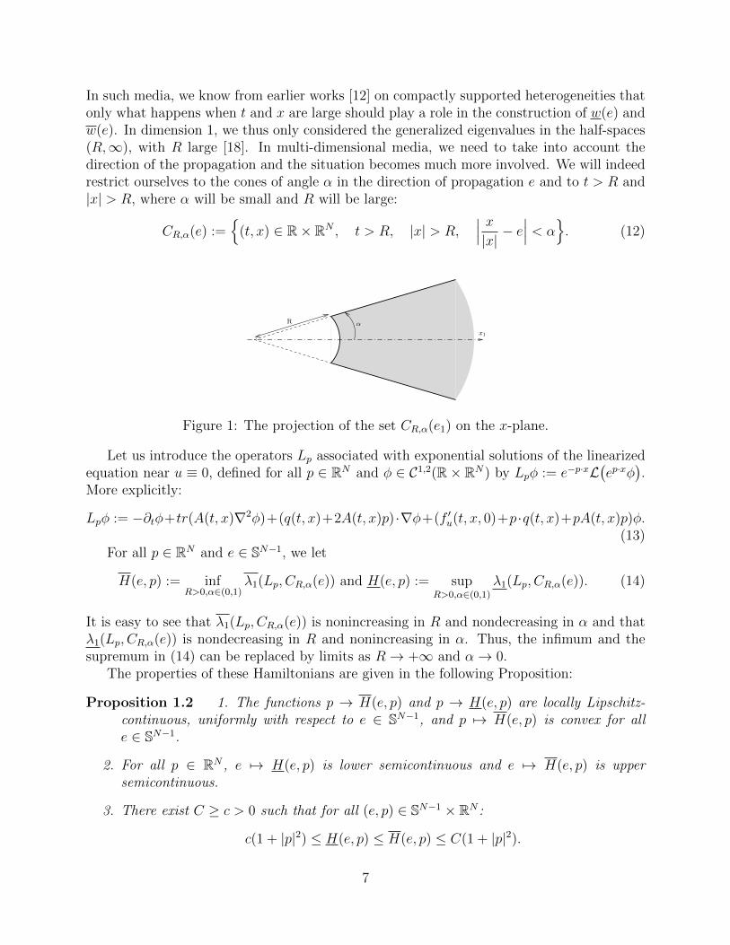
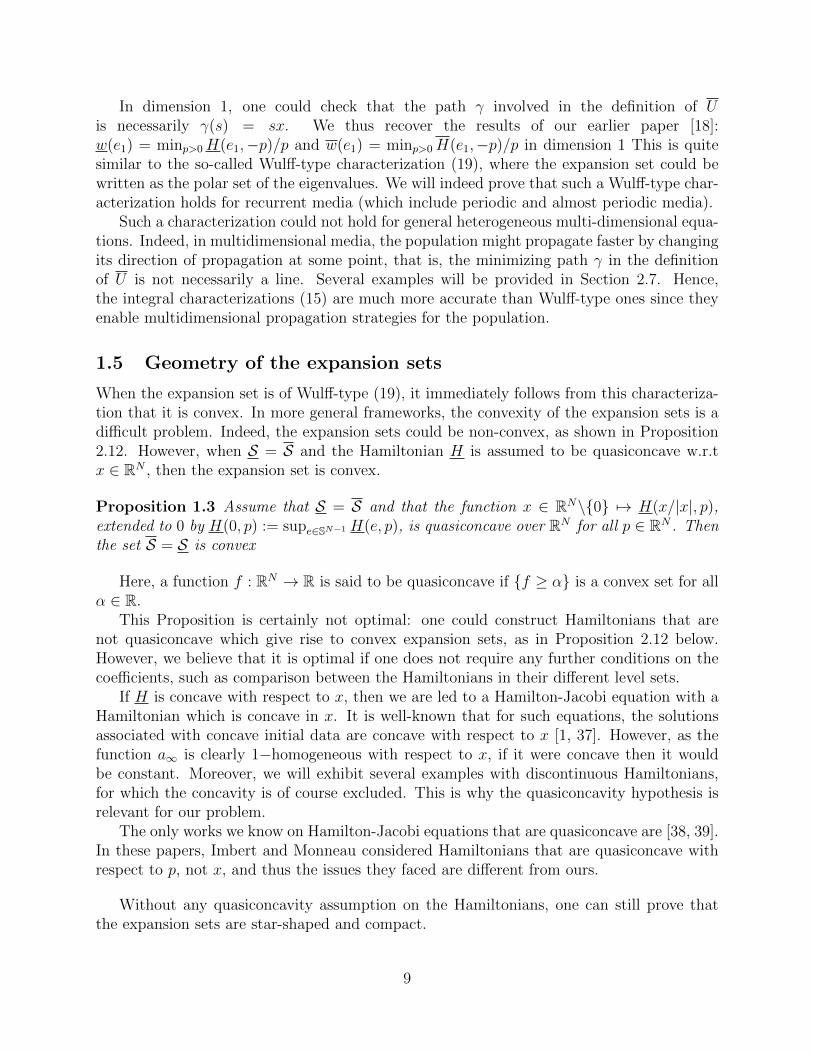
In such media, we know from earlier works [12] on compactly supported heterogeneities thatonly what happens when t and x are large should play a role in the construction of w(e) andw(e). In dimension 1, we thus only considered the generalized eigenvalues in the half-spaces(R,∞), with R large [18]. In multi-dimensional media, we need to take into account thedirection of the propagation and the situation becomes much more involved. We will indeedrestrict ourselves to the cones of angle α in the direction of propagation e and to t > R and|x| > R, where α will be small and R will be large:

CR,α(e) :=

(t, x) ∈ R× RN , t > R, |x| > R,∣∣∣ x|x| − e∣∣∣ < α

. (12)

R α

x1

Figure 1: The projection of the set CR,α(e1) on the x-plane.

Let us introduce the operators Lp associated with exponential solutions of the linearizedequation near u ≡ 0, defined for all p ∈ RN and φ ∈ C1,2(R× RN) by Lpφ := e−p·xL

(ep·xφ

).

More explicitly:

Lpφ := −∂tφ+tr(A(t, x)∇2φ)+(q(t, x)+2A(t, x)p) ·∇φ+(f ′u(t, x, 0)+p ·q(t, x)+pA(t, x)p)φ.(13)

For all p ∈ RN and e ∈ SN−1, we let

H(e, p) := infR>0,α∈(0,1)

λ1(Lp, CR,α(e)) and H(e, p) := supR>0,α∈(0,1)

λ1(Lp, CR,α(e)). (14)

It is easy to see that λ1(Lp, CR,α(e)) is nonincreasing in R and nondecreasing in α and thatλ1(Lp, CR,α(e)) is nondecreasing in R and nonincreasing in α. Thus, the infimum and thesupremum in (14) can be replaced by limits as R→ +∞ and α→ 0.

The properties of these Hamiltonians are given in the following Proposition:

Proposition 1.2 1. The functions p → H(e, p) and p → H(e, p) are locally Lipschitz-continuous, uniformly with respect to e ∈ SN−1, and p 7→ H(e, p) is convex for alle ∈ SN−1.

2. For all p ∈ RN , e 7→ H(e, p) is lower semicontinuous and e 7→ H(e, p) is uppersemicontinuous.

3. There exist C ≥ c > 0 such that for all (e, p) ∈ SN−1 × RN :

c(1 + |p|2) ≤ H(e, p) ≤ H(e, p) ≤ C(1 + |p|2).

7

We underline that the Hamiltonians H and H are not continuous with respect to e ingeneral (see the example of Proposition 2.10 below). This is the source of serious difficulties.

Using these Hamiltonians, we will now define two functions from which we derive theexpansion sets. Define the convex conjugates with respect to p:

H?(e, q) := supp∈RN

(p · q −H(e, p)

)and H

?(e, q) := sup

p∈RN

(p · q −H(e, p)

),

which are well-defined thanks to Proposition 1.2. Let

U(x) := inf maxt∈[0,1]

∫ 1

tH?(γ(s)|γ(s)| ,−γ

′(s))ds, γ ∈ H1([0, 1]), γ(0) = 0, γ(1) = x,

∀s ∈ (0, 1), γ(s) 6= 0

U(x) := inf maxt∈[0,1]

∫ 1

tH?( γ(s)|γ(s)|),−γ

′(s))ds, γ ∈ H1([0, 1]), γ(0) = 0, γ(1) = x,

∀s ∈ (0, 1), γ(s) 6= 0.

(15)We will show in Lemma 7.7 below that U is indeed a minimum, in other words, for all

x, there exists an admissible path γ from 0 to x minimizing the maximum over t ∈ [0, 1] ofthe integral.

We define our expansion sets in general heterogeneous media as

S := clU = 0 and S := U = 0. (16)

The reader might distinguish here representations formulas for the solutions of Hamilton-Jacobi equations. Indeed, the sets S and S are related to the zero sets of the solutions ofsuch equations. Such representations formulas are well-known for Hamilton-Jacobi equationswith continuous coefficients (see for example [28, 54]). This link will be described in Section7 below. We will make use of these formulas in order to derive properties of the expansionsets.

We are now in position to state our main result.

Theorem 1 Take u0 a measurable and compactly supported function such that 0 ≤ u0 ≤ 1and u0 6≡ 0 and let u the solution of the associated Cauchy problem (2). One has

for all compact set K ⊂ intS, limt→+∞

supx∈tK |u(t, x)− 1|

= 0,for all closed set F ⊂ RN\S, limt→+∞

supx∈tF |u(t, x)|

= 0.

(17)

In order to state this result in terms of speeds, define for all e ∈ SN−1:

w(e) = supw > 0, we ∈ S and w(e) = supw > 0, we ∈ S. (18)

Then it follows from Theorem 1 that

w(e) ≤ w∗(e) ≤ w∗(e) ≤ w(e).

8

In dimension 1, one could check that the path γ involved in the definition of Uis necessarily γ(s) = sx. We thus recover the results of our earlier paper [18]:w(e1) = minp>0H(e1,−p)/p and w(e1) = minp>0H(e1,−p)/p in dimension 1 This is quitesimilar to the so-called Wulff-type characterization (19), where the expansion set could bewritten as the polar set of the eigenvalues. We will indeed prove that such a Wulff-type char-acterization holds for recurrent media (which include periodic and almost periodic media).

Such a characterization could not hold for general heterogeneous multi-dimensional equa-tions. Indeed, in multidimensional media, the population might propagate faster by changingits direction of propagation at some point, that is, the minimizing path γ in the definitionof U is not necessarily a line. Several examples will be provided in Section 2.7. Hence,the integral characterizations (15) are much more accurate than Wulff-type ones since theyenable multidimensional propagation strategies for the population.

1.5 Geometry of the expansion sets

When the expansion set is of Wulff-type (19), it immediately follows from this characteriza-tion that it is convex. In more general frameworks, the convexity of the expansion sets is adifficult problem. Indeed, the expansion sets could be non-convex, as shown in Proposition2.12. However, when S = S and the Hamiltonian H is assumed to be quasiconcave w.r.tx ∈ RN , then the expansion set is convex.

Proposition 1.3 Assume that S = S and that the function x ∈ RN\0 7→ H(x/|x|, p),extended to 0 by H(0, p) := supe∈SN−1 H(e, p), is quasiconcave over RN for all p ∈ RN . Thenthe set S = S is convex

Here, a function f : RN → R is said to be quasiconcave if f ≥ α is a convex set for allα ∈ R.

This Proposition is certainly not optimal: one could construct Hamiltonians that arenot quasiconcave which give rise to convex expansion sets, as in Proposition 2.12 below.However, we believe that it is optimal if one does not require any further conditions on thecoefficients, such as comparison between the Hamiltonians in their different level sets.

If H is concave with respect to x, then we are led to a Hamilton-Jacobi equation with aHamiltonian which is concave in x. It is well-known that for such equations, the solutionsassociated with concave initial data are concave with respect to x [1, 37]. However, as thefunction a∞ is clearly 1−homogeneous with respect to x, if it were concave then it wouldbe constant. Moreover, we will exhibit several examples with discontinuous Hamiltonians,for which the concavity is of course excluded. This is why the quasiconcavity hypothesis isrelevant for our problem.

The only works we know on Hamilton-Jacobi equations that are quasiconcave are [38, 39].In these papers, Imbert and Monneau considered Hamiltonians that are quasiconcave withrespect to p, not x, and thus the issues they faced are different from ours.

Without any quasiconcavity assumption on the Hamiltonians, one can still prove thatthe expansion sets are star-shaped and compact.

9

Proposition 1.4 The sets S and S are compact, star-shaped with respect to 0, and containan open ball centered at 0.

2 Applications

2.1 Recurrent media

When the coefficients are recurrent, our definition of expansion sets simplifies to a Wulff-type construction, as in periodic media. However, in some situations exact spreading speedsmight not exist and S 6= S.

Definition 2.1 A uniformly continuous and bounded function g : R × RN → R is recur-rent with respect to (t, x) ∈ R × RN if for any sequence (tn, xn)n∈N in R × RN such thatg∗(t, x) = limn→+∞ g(tn + t, xn +x) exists locally uniformly in (t, x) ∈ R×RN , there exists asequence (sn, yn)n∈N in R×RN such that limn→+∞ g

∗(t−sn, x−yn) = g(t, x) locally uniformlyin (t, x) ∈ R× RN .

The heuristic meaning of this definition is that the patterns of the heterogeneities repeatat infinity. It is easy to check that homogeneous, periodic and almost periodic functionsare recurrent. We thus expect similar phenomena as in periodic media to arise, even ifthe recurrence property is much milder than periodicity. Indeed, some functions might berecurrent without being almost periodic, such as the function (see [80])

g(x) =sin t+ sin

√2t

|1 + eit + ei√

2t|.

Proposition 2.2 Assume that A, q and f ′u(·, ·, 0) are recurrent with respect to (t, x) ∈ R×RN .Then

S = x, ∀p ∈ RN , λ1(L−p,R×RN) ≥ p·x and S = x, ∀p ∈ RN , λ1(L−p,R×RN) ≥ p·x.(19)

Note that such a Wulff-type characterization of the expansion sets immediately impliesfor all e ∈ SN−1:

w(e) := minp·e>0

λ1(L−p,R× RN)

p · eand w(e) := min

p·e>0

λ1(L−p,R× RN)

p · e, (20)

that is:

∀w ∈[0, w(e)

), lim

t→+∞u(t, x+ wte) = 1 and ∀w > w(e), lim

t→+∞u(t, x+ wte) = 0,

locally uniformly with respect to x ∈ RN . Hence, this result exactly means that the transitionbetween 0 and 1, that is, the level sets of u(t, ·) are contained in

[w(e)t, w(e)t

]along direction

e at sufficiently large time t. Such a characterization of the spreading speeds is very close tothe one holding in periodic media (see (33) below).

10

We have constructed the two expansion sets S and S as precisely as possible. However,these two sets might be different, that is, there does not necessarily exist an exact spreadingspeed in recurrent media. For instance, in Example 2 below we exhibit a situation wherethe advection term is recurrent with respect to time and for which there exists a range ofspeeds (w∗, w

∗) such that for all w ∈ (w∗, w∗), if u is defined as in Theorem 2.2, then for all

e ∈ SN−1, the ω-limit set of the function t 7→ u(t, wte) is the full interval [0, 1]. From thisone sees that one cannot expect to describe the invasion by a single expansion set, hence theintroduction here of two expansion sets S and S.

2.2 Almost periodic media

An important class of recurrent coefficients is that of almost periodic functions, for whichwe will show that S = S. We will use Bochner’s definition of almost periodic functions:

Definition 2.3 [23] A function g : R × RN → R is almost periodic with respect to(t, x) ∈ R × RN if from any sequence (tn, xn)n∈N in R × RN one can extract a subsequence(tnk , xnk)k∈N such that g(tnk + t, xnk + x) converges uniformly in (t, x) ∈ R× RN .

Theorem 2 Assume that A, q and f ′u(·, ·, 0) are almost periodic with respect to (t, x) ∈ R×RN .Then S = S and

w(e) = w(e) = minp·e>0

λ1(L−p,R× RN)

p · e= min

p·e>0

λ1(L−p,R× RN)

p · e. (21)

This Theorem is an immediate corollary of Theorem 2.2 and the following result, whichis new and of independent interest. We will thus leave the proof of Theorem 2 to the reader.

Theorem 3 Assume that A, q and c are almost periodic, where c ∈ Cδ/2,δloc (R × RN) is agiven uniformly continuous function. Let L = −∂t + tr(A∇2) + q · ∇ + c. Then one hasλ1(L,R× RN) = λ1(L,R× RN).

This result is derived through exactly the same arguments as in the proof of Theorem2.4 of our earlier one-dimensional paper [18]. We will thus omit its proof.

Let us also mention here the works of Shen, who proved these spreading properties in theparticular case q ≡ 0, A = A(x) is periodic in x and f is limit periodic in t and periodic inx (Theorem 4.1 in [75]).

2.3 Asymptotically almost periodic media

If A ≡ IN , q ≡ 0 and f ′u(x, 0) = f0 + g(t, x), where g is a compactly supportedand continuous function, then the same arguments as in Section II.D.3 of [18] showthat λ1(Lp, CR,α) = λ1(Lp, CR,α) = |p|2 + f0 for all α when R is large enough. Hence

H(e, p) = H(e, p) = |p|2 + f0 and

∀e ∈ SN−1, w(e) = w(e) = w∗(e) = w∗(e) = 2√f0.

11

This is consistent with the result we derived from [12] in the Introduction, and even slightlymore general since we make no negativity assumption on b.

This result can indeed be generalized to the case where the coefficients converge to almostperiodic functions at infinity thanks to Theorem 1.

Proposition 2.4 Assume that there exist space-time almost periodic functions A∗, q∗ andc∗ such that

limR→+∞

supt≥R,|x|≥R

(|A(t, x)− A∗(t, x)|+ |q(t, x)− q∗(t, x)|+ |f ′u(t, x, 0)− c∗(t, x)|) = 0. (22)

Then H(e, p) = H(e, p) = λ1(L∗p,R× RN) for all p ∈ RN and

w(e) = w(e) = minp·e>0

λ1(L∗−p,R× RN)

p · e= min

p·e>0

λ1(L∗−p,R× RN)

p · e. (23)

where L∗ = −∂t + tr(A∗(t, x)∇2) + q∗(t, x) · ∇+ c∗(t, x) and L∗pφ = e−p·xL∗(ep·xφ).

The proof of this Proposition is similar to that of Proposition 2.6 of our previous work[18]. We will thus omit its proof.

2.4 Uniquely ergodic media

We now consider uniquely ergodic coefficients.

Definition 2.5 A uniformly continuous and bounded function f : RN → Rm is calleduniquely ergodic if there exists a unique invariant probability measure P on its hullHf := clτaf, a ∈ RN, where the closure is understood with respect to the locally uni-form convergence, and where the invariance is understood with respect to the translationsτaf(x) := f(x+ a) for all x ∈ RN .

Periodic, almost periodic and compactly supported functions are particular sub classesof the uniquely ergodic one. The Penrose tiling provides an example of a uniquely ergodicfunction which is not almost periodic [68] (see [56] for other examples).

The notion of unique ergodicity is commonly used in dynamical system theory since itprovides a uniformity convergence in the Birkhoff ergodic theorem. This yields the followingequivalent characterization (which is proved for example in Proposition 2.7 of [56]).

Proposition 2.6 Let f : RN → Rm a uniformly continuous and bounded function. Thefollowing assertions are equivalent:

• f is uniquely ergodic

• for any continuous function Ψ : Hf → R, the following limit exists uniformly withrespect to a ∈ RN :

limR→+∞

1

|BR(a)|

∫BR(a)

Ψ(τyf)dy.

12

Indeed, this limit is equal to P(Ψ).

The interest for reaction-diffusion equations with uniquely ergodic coefficients has raisedsince the 2000’s, when the case of periodic ones was completely understood. Shen hasinvestigated the existence of generalized transition wave solutions of Fisher-KPP equationswith time uniquely ergodic coefficients [76] (see also [60]). Matano conjectured the existenceof generalized transition waves (see Section 3.4 below and [9, 55]) and of spreading propertiesin Fisher-KPP equations with space uniquely ergodic coefficients in several conferences.

In the present paper, we show the existence of spreading properties for Fisher-KPPequations with space uniquely ergodic coefficients.

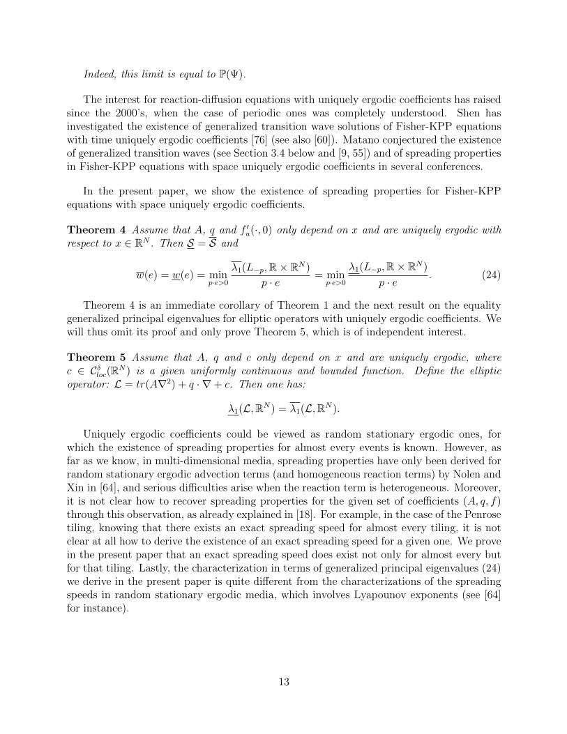
Theorem 4 Assume that A, q and f ′u(·, 0) only depend on x and are uniquely ergodic withrespect to x ∈ RN . Then S = S and

w(e) = w(e) = minp·e>0

λ1(L−p,R× RN)

p · e= min

p·e>0

λ1(L−p,R× RN)

p · e. (24)

Theorem 4 is an immediate corollary of Theorem 1 and the next result on the equalitygeneralized principal eigenvalues for elliptic operators with uniquely ergodic coefficients. Wewill thus omit its proof and only prove Theorem 5, which is of independent interest.

Theorem 5 Assume that A, q and c only depend on x and are uniquely ergodic, wherec ∈ Cδloc(RN) is a given uniformly continuous and bounded function. Define the ellipticoperator: L = tr(A∇2) + q · ∇+ c. Then one has:

λ1(L,RN) = λ1(L,RN).

Uniquely ergodic coefficients could be viewed as random stationary ergodic ones, forwhich the existence of spreading properties for almost every events is known. However, asfar as we know, in multi-dimensional media, spreading properties have only been derived forrandom stationary ergodic advection terms (and homogeneous reaction terms) by Nolen andXin in [64], and serious difficulties arise when the reaction term is heterogeneous. Moreover,it is not clear how to recover spreading properties for the given set of coefficients (A, q, f)through this observation, as already explained in [18]. For example, in the case of the Penrosetiling, knowing that there exists an exact spreading speed for almost every tiling, it is notclear at all how to derive the existence of an exact spreading speed for a given one. We provein the present paper that an exact spreading speed does exist not only for almost every butfor that tiling. Lastly, the characterization in terms of generalized principal eigenvalues (24)we derive in the present paper is quite different from the characterizations of the spreadingspeeds in random stationary ergodic media, which involves Lyapounov exponents (see [64]for instance).

13

2.5 Radially periodic media

We now consider coefficients that are periodic with respect to the radial coordinate r = |x|.As far as we know, this class of heterogeneity has never been investigated before.

Proposition 2.7 Assume that one can write

A(t, x) = aper(|x|)IN , q(t, x) = 0 and f ′u(t, x, 0) = cper(|x|)

where aper and cper are periodic with respect to r = |x|: there exists L > 0 such that for allr ∈ (0,∞):

aper(r + L) = aper(r) and cper(r + L) = cper(r).

For all p ∈ R, let:

Lperp φ := aper(r)φ′′ + 2paper(r)φ

′ +(p2aper(r) + cper(r)

)φ

and λper1 (Lperp ) the periodic principal eigenvalue associated with this operator.Then w(e) and w(e) do not depend on e and

w(e) = w(e) = minp>0

λper1 (Lper−p )

p.

The proof of this result is non-trivial since classical eigenvalues do not exist in thisframework. Hence, one more time the notions of generalized principal eigenvalues will beuseful. Moreover, the fact that only the heterogeneity of the coefficients in the truncatedcones CR,α(e) matters in the computation of these eigenvalues will also be needed.

2.6 Space independent media

When the coefficients only depend on t, the formulas for w(e) and w(e) are simpler. Forexample, if the coefficients are periodic in t, then the spreading speed is that associatedwith the average coefficients over the period. Our aim is to extend this property to generaltime-heterogeneous coefficients.

Proposition 2.8 Assume that A = IN , q ≡ 0 and f ′u(·, 0) do not depend on x. Then for alle ∈ SN−1,

w(e) = lim inft→+∞

infs>0

2

√1

t

∫ s+t

s

f ′u(s′, 0)ds′ (25)

w(e) = lim supt→+∞

sups>0

2

√1

t

∫ s+t

s

f ′u(s′, 0)ds′. (26)

The reader might easily check that the proof is also available when only q or A dependson t.

The existence of generalized transition waves in such media has been proved, under similarhypotheses as in the present paper, by the second author and Rossi [60]. The speed of these

14

fronts are determined through some upper and lower means of the coefficients that are verysimilar to the averaging involved in the definitions of w(e) and w(e).

When the coefficients are periodic in T , we recover that w(e) = w(e) is the spreadingspeed associated with the averaged reaction term. For general time-heterogeneous coeffi-cients, it is not always true that w(e) = w(e). This is because one can consider several waysof averaging. Indeed, our result is not optimal and it might be due to our choice of averaging(see Section 4 below).

However, when the coefficients admits a uniform mean value over R, then a variant ofour result gives w(e) = w(e) for all e. We can thus handle uniquely ergodic coefficients forexample. No such result exists in the literature as far as we know.

Proposition 2.9 Assume that A, q and f do not depend on x and that there exists〈A〉 ∈ SN(R), 〈q〉 ∈ RN and 〈c〉 ∈ R such that

limt→+∞

1

t

∫ a+t

a

A(s)ds = 〈A〉, limt→+∞

1

t

∫ a+t

a

q(s)ds = 〈q〉 and limt→+∞

1

t

∫ a+t

a

f ′u(s, 0)ds = 〈c〉

(27)uniformly with respect to a > 0. Then for all e ∈ SN−1,

w∗(e) = w∗(e) = w(e) = w(e) = 2√e〈A〉e〈c〉 − 〈q〉.

2.7 Directionally homogeneous media

We investigate in this Section the case where the coefficients converge in radial segmentsof R2. These types of heterogeneities give rise to very rich phenomena, such as non-convexexpansion sets.

We start with the case where the diffusion term converges in the half-spaces x1 < 0and x1 > 0

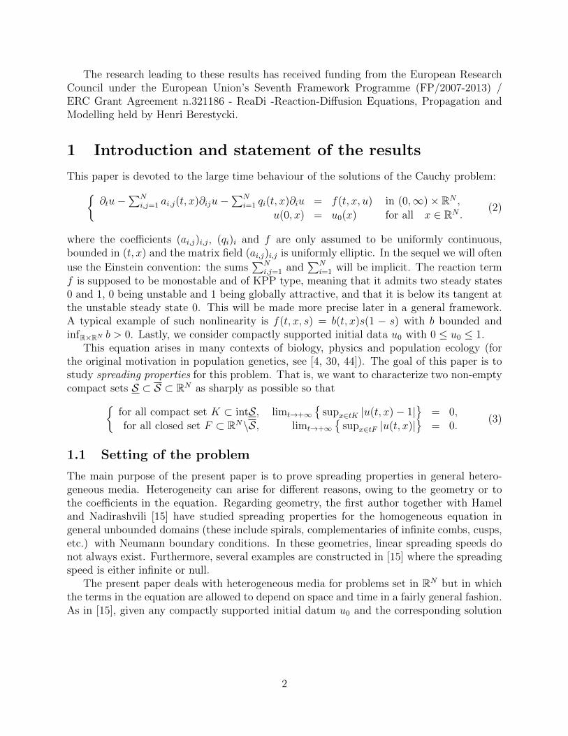
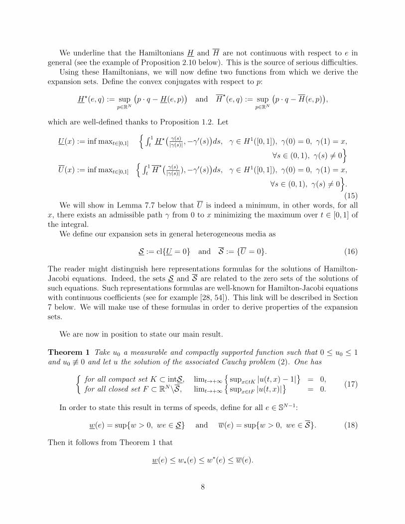
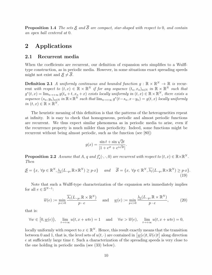
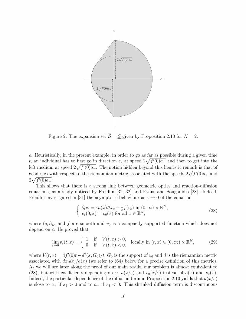
Proposition 2.10 Assume that N = 2, q ≡ 0, f does not depend on (t, x) andA(x1, x2) = a(x1)I2 is a smooth function such that limx1→±∞ a(x1) = a±, with a+ > a− > 0.Then S = S and this set is the convex envelope of

x ∈ R2, |x| ≤ 2√f ′(0)a+, x1 ≥ 0 ∪ x ∈ R2, |x| ≤ 2

√f ′(0)a−, x1 ≤ 0.

It is easy to compute that

H(e, p) = H(e, p) =

a+p

2 + f ′(0) if e1 > 0,a−p

2 + f ′(0) if e1 < 0.

Thus, when e1 < 0 and e1 6= −1, the spreading speed w∗(e) = w∗(e) is not equal to

v(e) = minp·e>0

H(e,−p)p · e

= 2√f ′(0)a−

and the expansion set is not obtained through a Wulff-type construction like (19). In otherwords, the spreading speed in direction e does not only depend on what happens in direction

15

2√f ′(0)a−

2√f ′(0)a+

Figure 2: The expansion set S = S given by Proposition 2.10 for N = 2.

e. Heuristically, in the present example, in order to go as far as possible during a given timet, an individual has to first go in direction e2 at speed 2

√f ′(0)a+ and then to get into the

left medium at speed 2√f ′(0)a−. The notion hidden beyond this heuristic remark is that of

geodesics with respect to the riemannian metric associated with the speeds 2√f ′(0)a+ and

2√f ′(0)a−.This shows that there is a strong link between geometric optics and reaction-diffusion

equations, as already noticed by Freidlin [31, 32] and Evans and Souganidis [28]. Indeed,Freidlin investigated in [31] the asymptotic behaviour as ε→ 0 of the equation

∂tvε = εa(x)∆vε + 1εf(vε) in (0,∞)× RN ,

vε(0, x) = v0(x) for all x ∈ RN ,(28)

where (aij)i,j and f are smooth and v0 is a compactly supported function which does notdepend on ε. He proved that

limε→0

vε(t, x) =

1 if V (t, x) > 0,0 if V (t, x) < 0,

locally in (t, x) ∈ (0,∞)× RN , (29)

where V (t, x) = 4f ′(0)t−d2(x,G0)/t, G0 is the support of v0 and d is the riemannian metricassociated with dxidxj/a(x) (we refer to (64) below for a precise definition of this metric).As we will see later along the proof of our main result, our problem is almost equivalent to(28), but with coefficients depending on ε: a(x/ε) and v0(x/ε) instead of a(x) and v0(x).Indeed, the particular dependence of the diffusion term in Proposition 2.10 yields that a(x/ε)is close to a+ if x1 > 0 and to a− if x1 < 0. This shrinked diffusion term is discontinuous

16

and, more important, the rescaled initial datum v0(x/ε) becomes very singular when ε→ 0,unlike the smooth one in Freidlin’s problem (28). Thus we could not directly apply Freidlin’sresult. However, we will find at an intermediate step a characterization of the expansion setwhich is close to Freidlin’s (29), which is not surprising. We will then explicitly compute thegeodesics, which makes another difference with earlier papers on the link between geometricoptics and Hamilton-Jacobi equations. Computing these geodesics, we will recover someSnell-Descartes law (see the Remark below the proof of Proposition 2.10).

In order to prove Theorem 1, we will determine the limit of the function uε(t, x) = u(t/ε, x/ε),where u satisfies (2) (see below). The function uε satisfies an equation similar to (28) exceptthat the initial datum vε(x) = u0(x/ε) depends on ε and that a(x) is replaced by a(x/ε).But the definition of a in Proposition 2.10 yields that a(x/ε) − a(x) → 0 as x1 → ±∞.Hence, if a is very close to a step function x 7→ a+1x1>0 + a−1x1<0, then uε and vε might beclose for all ε > 0 and one could try to prove Proposition 2.10 using the same arguments asin [31].

However, there are several important differences between [31] and our approach. First,we use here a direct and general approach: Theorem 1 holds even when a(x) and a(x/ε)are not close (for example for periodic or almost periodic functions a). Next, the explicitcomputation of the riemannian metric associated with dxidxj/a(x) when a is a step functionis completely new as far as we know.

Next, let consider the same framework but with f depending on x1 instead of a.

Proposition 2.11 Assume that N = 2, q ≡ 0, A = I2 and f(t, x, s) = c(x1)s(1− s), wherec is a smooth function such that limx1→±∞ c(x1) = µ±, with µ+ > µ− > 0.

Then S = S and this set is the convex envelope of

x ∈ R2, |x| ≤ 2√µ+, x1 ≥ 0 ∪ x ∈ R2, |x| ≤ 2

√µ−, x1 ≤ 0.

Surprisingly, the functions U and U are quite different from the ones arising along theproof of Proposition 2.10. However, their level-sets S = U = 0 and S = clU = 0 arevery similar to that of Proposition 2.10 and we find the same type of picture as Figure 2.7.

If A(t, x) = a(x1)IN and if there exist two periodic functions x1 7→ a+(x1) andx1 7→ a−(x1) such that a(x1) − a±(x1) → 0 as x1 → ±∞, then it does not seem possi-ble to write the expansion set as the convex hull of two half-circles as in Proposition 2.10holds in general. Indeed, the proof of Proposition 2.10 relies on the particular structure ofthe Hamiltons H(e, p) and H(e, p), which are quadratic polynoms with respect to p for all e.

We also mention here the recent work of Roquejoffre, Rossi and the first author [20] on acoupled reaction-diffusion modeling the diffusion of a species along a line. Computing theirexpansion set, the authors faced similar problems but found a picture quite different fromFigure 2.7.

If a converges to a− in a smaller part of R2 than a half-space, then the expansion set isnot as in Proposition 2.10.

17

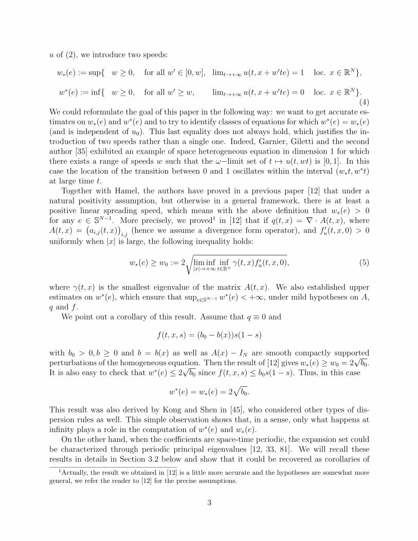
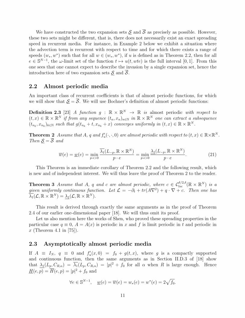
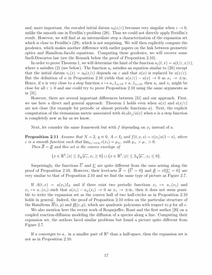
Proposition 2.12 Assume that N = 2, q ≡ 0, f does not depend on (t, x) andA(x) = a(x)I2 is a smooth function such that

limx1→+∞

a(x1, αx1) =

a+ if |α| < r0

a− if |α| > r0

where a+ > a− > 0 and 0 < r0 < r :=√

a−a+−a− Then S = S and this set is:

|x| < 2

√f ′(0)a+, |x2| ≥ r0x1

∪x1 <

1− r0r

r0 + r|x2|+

2√f ′(0)a+(1 + r2

0)

1 + r0/r, |x2| ≤ r0x1

.

This expansion set is non-convex if r0r < 1, as displayed in the Figure illustrating Propo-sition 2.12.

2√f ′(0)a+

2√f ′(0)a+(1 + r2

0)

1 + r0/rarctan r0

Figure 3: The non-convex expansion set S = S given by Proposition 2.12.

This is the first time, as far as we know, that a reaction-diffusion giving rise to a non-convex expansion set is exhibited. Indeed, for all the classes of heterogeneities previouslyinvestigated in the literature, the expansion sets were characterized through a Wulff-typeconstruction (35), which is clearly convex. Thus the investigation of more general types ofheterogeneities was needed in order to find non-convex expansion sets.

As a conclusion, if N = 2, q ≡ 0, f does not depend on (t, x) and A(x) = a(x)IN , where aconverges to some limit function a∞(x) in a finite number of radial segments, then Proposition11.1 below yields that S = S. Hence, if in addition a∞ is assumed to be quasiconcave, thenthe reader can check that Proposition 1.3 yields that S is convex. However, this result isnot optimal since, for example, under the assumptions of Proposition 2.12, one would obtainthe function a∞(x) = a+ if |x2| > r0x1, a∞(x) = a+ if |x2| < r0x1, which is not quasiconcavesince r0 > 0, however the expansion set is convex if r0r ≥ 1.

18

3 Earlier works in the homogeneous, periodic and ran-

dom stationary ergodic cases

We recall in this Section some earlier works and show that in homogeneous and periodicframeworks, these results could be recovered through Theorem 1. As we have already de-scribed in details how to carry out such a verification in dimension 1 (see Sections II.D.1and 3 in [18]), we leave the proofs to the reader in the present article. We also mention thecase of random stationary ergodic coefficients, for which the existence of an exact spreadingspeed has been proved in various particular contexts in earlier works, but for which it is notclear whether our method is close from an optimal result or not in multi-dimensional media.

3.1 Homogeneous equation

Let first recall some well-known results in the case where the coefficients do not depend on(t, x). In this case, equation (2) is indeed the the classical homogeneous equation

∂tu−∆u = f(u), (30)

where f(0) = f(1) = 0 and f(s) > 0 if s ∈ (0, 1), which has been widely studied. Whenlim infs→0+ f(s)/s1+2/N > 0, a classical result due to Aronson and Weinberger [4] yields thatthere exists w∗ > 0 such that the solution u of the Cauchy problem associated with a givennon-null compactly supported initial datum satisfies

lim inft→+∞

inf|x|≤wt

u(t, x) = 1 if 0 ≤ w < w∗,

limt→+∞

sup|x|≥wt

u(t, x) = 0 if w > w∗.(31)

In other words S = S = x, |x| ≤ w∗. Moreover, w∗ is also characterized as the minimalspeed of travelling fronts solutions, defined in [4, 44], and this speed is exactly w∗ = 2

√f ′(0)

for KPP nonlinearities, that is, for nonlinearities f satisfying f(s) ≤ f ′(0)s for all s ≥ 0 (see[4]).

When the nonlinearity is of KPP type, these results could be derived from Theorem 1and Proposition 2.2. Indeed, homogeneous coefficients are obviously recurrent and one hasλ1(Lp,RN) = λ1(Lp,RN) = f ′(0) + |p|2. Hence, (19) reads S = S = x, |x| ≤ w∗.

3.2 Periodic media

Let us consider the case where all the coefficients ai,j, qi and f are space-time periodiccoefficients. A function h = h(t, x) is called space-time periodic if there exist some positiveconstants T, L1, ..., LN so that

h(t, x) = h(t, x+ Liεi) = h(t+ T, x)

for all (t, x) ∈ R × RN , where (εi)i is a given orthonormal basis of RN . The periodsT, L1, ..., LN will be fixed in the sequel. Periodicity is understood to mean the same pe-riod(s) for all the terms.

19

The spreading properties in space periodic media have first been proved using probabilis-tic tools by Freidlin and Gartner [33] in 1979 and Freidlin [32] in 1984, when the coefficientsonly depend on x. These properties have been extended to space-time periodic media byWeinberger in 2002 [81], using a rather elaborate discrete formalism. Two alternative proofsof spreading properties in multidimensional space-time periodic media have been given bythe authors of the present paper, together with Hamel, in [12] (see also [59, 62]). Thesemethods both use accurate properties of the periodic principal eigenvalues associated withthe linearized equation at 0. Lastly, Majda and Souganidis [54] proved some homogenizationresults that are very close, but different, from spreading properties in the space-time periodicsetting (we make this connection clear in Section 5).

In periodic media, the asymptotic spreading speed depends on the direction of propaga-tion. Thus, the property proved in [12, 32, 33, 81] is the existence of an asymptotic directionalspreading speed w∗(e) > 0 in each direction e ∈ SN−1, so that for all initial datum u0 6≡ 0,0 ≤ u0 ≤ 1 with compact support, one has lim inf

t→+∞u(t, x+ wte) = 1 if 0 ≤ w < w∗(e),

limt→+∞

u(t, x+ wte) = 0 if w > w∗(e),(32)

locally in x ∈ RN . It is possible to characterize w∗(e) in terms of periodic principal eigen-values in the KPP case, that is, when f(t, x, s) ≤ f ′u(t, x, 0)s for all (t, x, s) ∈ R×RN ×R+.Namely, let L the parabolic operator associated with the linearized equation near 0:

Lφ := −∂tφ+ ai,j(t, x)∂ijφ+ qi(t, x)∂iφ+ f ′u(t, x, 0)φ,

and let Lpφ := e−p·xL(ep·xφ) for all p ∈ RN . We know from the Krein-Rutman theory thatthe operator Lp admits a unique periodic principal eigenvalue kperp , that is, an eigenvalueassociated with a periodic and positive eigenfunction. Then the characterization proved byFreidlin and Gartner [32, 33] in the space periodic framework and extended to space-timeperiodic frameworks in [12, 81] reads

w∗(e) = minp·e>0

kper−pp · e

. (33)

This quantity can also be written using the minimal speed of existence of pulsating travellingfronts (defined and investigated in [8, 14, 16, 29, 59, 62, 81]), which is indeed the appropriatecharacterization when f is not of KPP type [81].

Lastly, Weinberger [81] proved that the convergence (32) is uniform in all directions,meaning that

for all compact set K ⊂ intS, limt→+∞

supx∈tK |u(t, x)− 1|

= 0,for all closed set F ⊂ RN\S, limt→+∞

supx∈tF |u(t, x)|

= 0,

(34)

withS = x, ∀p ∈ RN , kper−p ≥ p · x. (35)

20

Of course, as for all e ∈ SN−1 and w > 0, we ∈ S if and only if w < w∗(e), we recover (32)as a corollary of (34). This set is the polar set of A = p/kper−p , p ∈ RN and, by analogywith crystallography2, the set S is sometimes called the Wulff shape of equation (2).

In this framework, the same type of arguments as in our previous one-dimensional paper[18] yield that λ1(Lp,RN) = λ1(Lp,RN) = kperp . Hence, as periodicity implies recurrency,Proposition 2.2 leads to (35).

3.3 Random stationary ergodic framework

The first proof of the existence of an exact spreading speed in random stationary ergodicmedia goes back to the pioneering papers of Freidlin and Gartner [33] and Freidlin [32], whoconsidered time-independent reaction terms in dimension 1 using large deviation techniques.In multi-dimensional media, the existence of an exact spreading speed has been proved byNolen and Xin for space-time heterogeneous advection terms and homogeneous reactionterms [64, 65, 66]. As they claimed in [64], their approach should work when the diffusionterm is also space-time random stationary ergodic.

In these cases, the exact asymptotic spreading speed is characterized through some Lya-pounov exponents associated with the underlying Brownian process. Similar quantities ap-pear in related problems such as homogenization of reaction-diffusion equations (see [52] andthe references therein). The connections between these various approaches will be discussedin details in Section 5.

In our earlier paper [18], we have exhibited an alternative definition in dimension 1,close from an alternative one-dimensional characterization due to Freidlin [32] but involvinggeneralized principal eigenvalues, and we have proved the existence of an exact spreadingspeed for random stationary ergodic diffusion and reaction terms. We used in our earlierone-dimensional paper [18] a different definitions for the generalized principal eigenvalues.Namely, in [18] we only asked the test-functions defining the generalized principal eigenvaluesin Definition 1.1 to satisfy a sub-exponential growth at infinity lim|x|→+∞

1|x| lnφ(x) = 0,

which is of course less restrictive than asking φ ∈ L∞ and inf φ > 0. This relaxed definitionenabled us to construct exact eigenfunctions associated with our generalized eigenvalues inthe random stationary ergodic framework, from which the existence of an exact spreadingspeed followed. Unfortunately, in the present paper we were not able to construct exacteigenfunctions with sub-exponential growth at infinity in dimension N , since the method weused in [18] relied on one-dimensional arguments.

The introduction of a “metric problem” formulation by Armstrong and co-authors [2, 3]allowed for a new approach in homogenization theory. This “metric problem” provides anexact corrector in RN\B1. Our point of view bear some similarities with this approach inthat our approximate correctors are only required to satisfy the equation in truncated conesCR,α(e). The methods developed in [2, 3] might provide a path towards the construction ofexact correctors. We leave these possible extensions as open problems.

We underline that all these earlier papers made some stationarity hypothesis on the ran-dom heterogeneity, which means that the statistical properties of the medium do not depend

2In [82], Wulff proved that for a given crystal volume, the set that minimizes the surface energy isW = x, x · e ≤ σ(e) for all e ∈ SN−1, where σ is the surface tension.

21

on time and space. Many classes of deterministic coefficients could indeed be turned into arandom stationary ergodic setting so that the orginal deterministic media is a given event.This a well-known fact for periodic, almost periodic (see [67]) and uniquely ergodic deter-ministic coefficients. In such setting, one could thus derive spreading properties for almostevery event. However, it is not always clear whether these spreading properties hold for theoriginal deterministic equation or not. Indeed, if the deterministic coefficients have a com-pactly supported heterogeneity (see below for a precise definition), then this approach givesa trivial result: the homogeneous equation associated with translations at infinity verifies aspreading property. But it does not give any result concerning the original heterogeneousequation. Hence, even if one can transform deterministic heterogeneous equations into ran-dom stationary ergodic ones, it might be difficult to check that this probabilistic setting isuseful to prove spreading properties for the original deterministic equation.

3.4 The link between travelling waves and spreading properties

Let us conclude this Introduction with a few words about travelling waves. We have re-called above that in homogeneous and periodic media, there is an explicit link between theasymptotic spreading speed and the minimal speed of existence of travelling waves. Forexample, these two quantities are equal in dimension 1. This is why most of the papersaddress propagation problems using both notions indistinctly.

In general heterogeneous media, the first author and Hamel [9, 10] and Matano [55]have introduced two generalizations of the notion of travelling wave. Several recent papers[9, 10, 11, 57, 58, 63, 74, 85] investigate the existence, uniqueness and stability of such wavesin the case when the nonlinearity is bistable or of ignition type and in dimension 1. Inhigher dimensions, for the same types of nonlinearities, Zlatos has found new existence andnon existence results (see [86] and references therein).

When the nonlinearity is monostable and time-heterogenous, the existence of generalizedtransition waves has been proved by the second author and Rossi [60]. It is not true ingeneral that such waves exist for space-heterogeneous monostable equations. In fact, Nolen,Roquejoffre, Ryzhik and Zlatos [61] construct a counter-example for a compactly supportedheterogeneity. Zlatos further provided conditions in this framework ensuring the existenceof generalized transition waves [84].

Hence, for some classes of heterogeneities, there exists an exact asymptotic spreadingspeed but generalized transition waves do not exist. This emphasizes that one needs to becareful and to distinguish between the two approaches in general heterogeneous media.

4 Further examples and discussion

In order to conclude the statement of the results, we discuss their optimality analyzing indetail various examples.

22

4.1 An example of recurrent media which does not admit an exactspreading speed

We have described in Section 2.1 how the results simplify when the coefficients are recurrent.Then we applied these results to various classes of recurrent media, such as homogeneous,periodic and almost periodic ones, for which we have proved that w(e) = w(e), showingthat there exists an exact asymptotic spreading speed in every directions. It could thusbe tempting to conjecture that any equation with recurrent coefficients admits an exactasymptotic spreading speed in every directions. We will indeed construct a counter-exampleto this conjecture.

The next Proposition gives a generic way to construct examples for which w∗(e) < w∗(e).We recall here that another such example was provided by the second author, together withGarnier and Giletti [35], for an equation with a non-recurrent reaction term depending on x(but not on t). Proposition 4.1 is proved in Section 10 below.

Proposition 4.1 Consider a uniformly continuous and bounded function ω ∈ Cδloc(R) andlet

ω = lim supT→+∞

1

T

∫ T

0

ω(t)dt and ω = lim infT→+∞

1

T

∫ T

0

ω(t)dt.

Let e ∈ SN−1, consider a bounded, nonnegative, mesurable and compactly supported functionu0 6≡ 0 and let u the solution of the Cauchy problem

∂tu−∆u− ω(t)e · ∇u = u(1− u) in (0,∞)× RN ,u(0, x) = u0(x) in RN .

(36)

Then if ω − ω < 4, one has

w∗(e) = 2 + ω and w∗(e) = 2 + ω.

Moreover, if w ∈ (w∗(e), w∗(e)), then for all s ∈ [0, 1], there exists a sequence tn → +∞

such that u(tn, wtne)→ s as n→ +∞.

Example 1. Let first construct an explicit example of non-recurrent coefficients forwhich w∗(e) < w∗(e). Consider the same equation as in Proposition 4.1 with

ω(t) =

ω2 if t ∈ [sn + 1, tn],ω1 if t ∈ [tn + 1, sn+1],

where (sn)n≥1 and (tn)n≥1 are two sequences of R+ such that tn− sn = n and sn+1− tn = n,0 < ω1 < ω2 < 4 + ω1, ω is smooth and ω(t) ∈ [ω1, ω2] for all t ∈ R. Then it follows fromProposition 4.1 that w∗(e) = 2 + ω1 and w∗(e) = 2 + ω2. Moreover, one easily computesusing the Remark below Proposition 2.8 that w(e) = 2 + ω1 and w(e) = 2 + ω2. Thus, inthis case, w∗(e) < w∗(e) but our result is optimal since w(e) = w∗(e) and w(e) = w∗(e).

Example 2. Let now construct a similar example but with recurrent coefficients. Ithas long been known that recurrent functions do not necessarily admit a mean value, but

23

there does not exist many explicit examples in the literature. One was exhibited by Lewinand Lewitan in 1939 [49]. Let ω such a function: ω is uniformly continuous, bounded anddepends recurrently on t, and one has

lim infT→+∞

1

T

∫ T

0

ω(t)dt < lim supT→+∞

1

T

∫ T

0

ω(t)dt.

Under the same hypotheses as in Proposition 4.1, one then immediatley gets w∗(e) < w∗(e),that is, equation (36) does not admit an exact spreading speed in direction e, despite it hasrecurrent coefficients.

In these Examples, as in [35], the spreading is not linear: the level lines of u(t, ·) do notmove with a given speed but oscillate between two speeds. Hence, instead of consideringthe limit of t 7→ u(t, wte) with w ∈ R+, one should try to localize the level sets of u(t, ·)by computing the limit of t 7→ u

(t, e∫ t

0w(s)ds

), with w ∈ C0(R+,R+). We introduced with

Hamel some notions that are useful when one tries to identify such “nonlinear” spreadingproperties in [12]. The method we present in this paper only fits to the investigation of“linear” spreading properties. We hope to be able to prove the existence of spreading surfaces(see [12]) involving generalized principal eigenvalues in a forthcoming work.

4.2 A time-heterogeneous example where our construction is notoptimal

In the next example, Proposition 4.1 shows that w∗(e) = w∗(e), that is, there exists an exactspreading speed, but the speeds we construct through Theorem 1 are not equal: w(e) < w(e).Thus, Theorem 1 do not give optimal bounds on the level sets of u(t, ·) in this case.

Example 3. Consider the same ω as in Example 1 but with sn+1 − tn = n2. Then onone hand, Proposition 4.1 gives

w∗(e) = w∗(e) = 2 + ω1 since1

t

∫ t

0

ω(s)ds→ ω1 as t→ +∞.

On the other hand, one can easily prove that

lim supt→+∞

sups>0

1

t

∫ s+t

s

ω = ω2 and lim inft→+∞

infs>0

1

t

∫ s+t

s

ω = ω1.

The Remark below Proposition 2.8 gives

w(e) = 2 + ω1 = w∗(e) and w(e) = 2 + ω2 > w∗(e).

4.3 A multi-dimensional example where our construction is notoptimal

We conclude with an example showing that our construction of w(e) might not be optimalin dimension N . In this example a direct approach, through sub and supersolutions, givesmore accurate results.

24

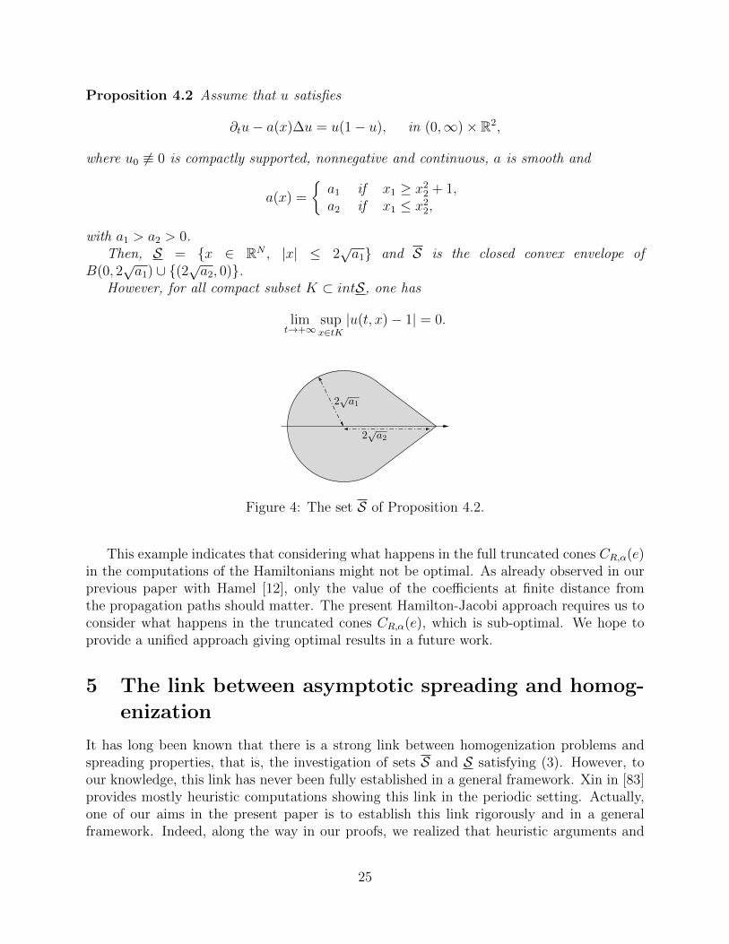
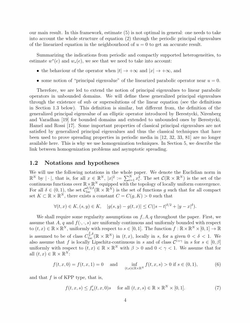
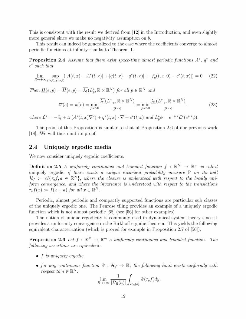
Proposition 4.2 Assume that u satisfies

∂tu− a(x)∆u = u(1− u), in (0,∞)× R2,

where u0 6≡ 0 is compactly supported, nonnegative and continuous, a is smooth and

a(x) =

a1 if x1 ≥ x2

2 + 1,a2 if x1 ≤ x2

2,

with a1 > a2 > 0.Then, S = x ∈ RN , |x| ≤ 2

√a1 and S is the closed convex envelope of

B(0, 2√a1) ∪ (2√a2, 0).

However, for all compact subset K ⊂ intS, one has

limt→+∞

supx∈tK|u(t, x)− 1| = 0.

2√a1

2√a2

Figure 4: The set S of Proposition 4.2.

This example indicates that considering what happens in the full truncated cones CR,α(e)in the computations of the Hamiltonians might not be optimal. As already observed in ourprevious paper with Hamel [12], only the value of the coefficients at finite distance fromthe propagation paths should matter. The present Hamilton-Jacobi approach requires us toconsider what happens in the truncated cones CR,α(e), which is sub-optimal. We hope toprovide a unified approach giving optimal results in a future work.

5 The link between asymptotic spreading and homog-

enization

It has long been known that there is a strong link between homogenization problems andspreading properties, that is, the investigation of sets S and S satisfying (3). However, toour knowledge, this link has never been fully established in a general framework. Xin in [83]provides mostly heuristic computations showing this link in the periodic setting. Actually,one of our aims in the present paper is to establish this link rigorously and in a generalframework. Indeed, along the way in our proofs, we realized that heuristic arguments and

25

homogenization methods need to be supplemented in order to derive the actual spreadingproperties for reaction-diffusion equations.

Let us now describe this more precisely. Consider a solution u of the nonlinear reaction-diffusion equation (2). In order to locate its level sets, following the homogenization ap-proach, one lets Zε(t, x) := ε lnu(t/ε, x/ε). The aim is then to compute its limit when itexists. This function satisfies

∂tZε − ε∑N

i,j=1 ai,j(t/ε, x/ε)∂ijZε −H(t/ε, x/ε,∇Zε)= 1

vεf(t/ε, x/ε, vε)− f ′u(t/ε, x/ε, 0) in (0,∞)× RN ,

Zε(0, x) =

ε lnu0(x/ε) if u0(x/ε) 6= 0,−∞ otherwise,

withH(s, y, p) := pA(s, y)p+ q(s, y) · p+ f ′u(s, y, 0).

If one replaces the initial datum by a function which does not depend on ε and if theright-hand side cancels, that is, if f = f(t, x, u) is linear with respect to u, then this equationreduces to the following typical equation considered in the homogenization literature:

∂tZε − κεai,j(t/ε, x/ε)∂i,jZε −H(t/ε, x/ε,∇Zε) = 0 in (0,∞)× RN ,Zε(0, x) = Z0(x) otherwise,

(37)

with κ = 1 here. Such problems are usually investigated in the framework whereZ0 ∈ Cb(RN), κ ≥ 0 and H is continuous in (t, x, p), convex in p and H(t, x, p)/|p| → +∞ as|p| → +∞ uniformly in (t, x) ∈ R× RN (see for instance [52]).

Consider first the case when H is periodic in x and does not depend on t. The heuristicsthat give the characterization of the effective Hamiltonian Hhom are the following (we referto [52] for a complete review on this topic). First, one looks for an approximation of theform

Zε(t, x) ' Z(t, x) + εY (t, x, x/ε),

where Y is periodic in x/ε. Then, in order to separate the two scales x and x/ε, a straight-forward computation shows that Y has to satisfy an equation of the form

−κ∆yY +H(y,∇xZ +∇yY ) = Hhom(∇xZ)

for some function Hhom. In other words, choosing (t, x) and letting p = ∇xZ(t, x) andvp(y) = Y (t, x, y), one needs to find for all p ∈ RN a solution

(vp, H

hom(p)), with vp periodic,

of−κ∆yvp +H(y, p+∇yvp) = Hhom(p) in RN . (38)

This equation is called the cell problem associated with (37) and vp is called an exact correctorassociated with this cell problem. If H(y, p) = |p|2+c(y) and κ = 1, which is the Hamiltonianthat comes from a linear elliptic equation equation, using the WKB change of variableφp = e−vp , we see that the existence of an exact corrector is equivalent to the existence of aperiodic solution (φp, H

hom(p)) of

∆yφp + 2p · ∇φp + (|p|2 + c(y))φp = Hhom(p)φp in RN . (39)

26

In other words, as φp > 0, in this case Hhom(p) is the periodic principal eigenvalue associatedwith the operator Lp = ∆ + 2p · ∇ + (|p|2 + c(y)). Indeed, it is always possible to find asolution (vp, H

hom(p)) of the more general cell problem (38) when the Hamiltonian H(y, p)is periodic in y. Then, a classical machinery yields that limε→0 Zε(t, x) = Z(t, x) locally in(t, x), where Z is the unique solution of the homogenized equation

∂tZ −Hhom(∇Z) = 0 in (0,∞)× RN ,Z(0, x) = Z0(x) otherwise.

(40)

When H is almost periodic, it is not always true that there exists a principal eigenvalue,and thus an exact corrector, associated with Lp. This problem was solved by Ishii [43] whenκ = 0 and by Lions and Souganidis [51] for fully nonlinear almost periodic equations. Theyintroduced the notion of approximate correctors. Namely, they proved the existence of aconstant Hhom(p) such that for all δ > 0, there exist two bounded functions vδp and vp,δ thatsatisfy in RN :

−κ∆yvp,δ+H(y, p+∇yvp,δ) ≤ Hhom(p)+δ and −κ∆yvδp+H(y, p+∇yv

δp) ≥ Hhom(p)−δ.

(41)The existence of approximate correctors is sufficient in order to homogenize equation (37),as proved in [43, 51]. Now, if H(y, p) = |p|2 + c(y) and κ = 1, letting φp,δ = exp(−vp,δ) andφδp = exp(−vδp), the existence of approximate correctors is equivalent to the existence of φp,δand φδp such that

Lpφp,δ ≥ (Hhom(p)− δ)φp,δ and Lpφδp ≤ (Hhom(p) + δ)φδp in RN ,

where φp,δ and φδp are bounded and have a positive infimum. In other words, in terms of thegeneralized principal eigenvalues we have defined here, there exist approximate correctors ifand only if

λ1(Lp,R× RN) = λ1(Lp,R× RN).

Ishii [43] and Lions and Souganidis [51] obtained such approximate correctors in thespace almost periodic framework using Evan’s perturbed test function method, that wasfirst introduced in a periodic framework [27]. We also made use of this method to prove theequality of the two generalized principal eigenvalues in space-time almost periodic media in[18].

When H is random stationary ergodic with respect to x, it has been proved independentlyby Lions and Souganidis [52] and by Kosygina, Rezakhanlou and Varadhan [46] that it ispossible to homogenize (37), that is, Zε(t, x) → Z(t, x) as ε → 0 locally uniformly in (t, x)almost surely and the limit Z satisfies a deterministic equation of the form (40). Thisresult has been extended to space-time random stationary ergodic equations by Kosyginaand Varadhan [47] (see also [70] when κ = 0).

It is not always true that there exist approximate correctors in random stationary er-godic media. Lions and Souganidis [52] proved that there exists a global subsolution v of−κ∆v + H(x, p + ∇v) ≤ Hhom(p) in RN almost surely, where ∇v is a random stationaryergodic function with mean 0. It is well-known that such a function needs not necessarilybe bounded nor stationary anymore but that it is sub-linear at infinity: v(x)/|x| → 0 as

27

|x| → +∞ almost surely. Hence, one needs to extend the notion of approximate correctorsto sublinear functions at infinity. Moreover, even with this extended notion, it is not alwaystrue that there exists an upper approximate corrector. Indeed, Lions and Souganidis pro-vided a counter-example in [50]. This is why they proposed a new notion of correctors (seeProposition 7.3 in [52]), which is tailored for homogenization problems of random stationaryergodic equations.

However, in dimension 1, for second order linear elliptic equations, we have proved in ourearlier paper [18] that there exists an approximate corrector almost surely (see also [26] fora similar result concerning 1D first order nonlinear Hamilton-Jacobi equations). We thusderived the equality of the two generalized principal eigenvalues, providing we relax theirdefinitions in order to only require a sublinear growth at infinity of the test-functions, and theexistence of an exact asymptotic spreading speed. We were not able to extend this result tomulti-dimensional equations and leave such a generalization as an important open problem.

As far as we know, homogenization results for (37) have never been investigated whenthe dependence of H with respect to x is general. Indeed, it is not possible to prove thatthe family (Zε)ε>0 converges in general (see Proposition 4.1 above for example). The recentpapers [46, 47, 52, 70] addressing this question focused on random stationary ergodic Hamil-tonians H, but not all deterministic equations could be transformed into a relevant randomstationary ergodic one, as already described in Section 3.3.

Thus, it is only possible to obtain bounds on the spreading speeds w∗(e) and w∗(e) fora general heterogeneous equation. Of course, we aim at constructing bounds as preciselyas possible. In particular we identify some classes of equations where our bounds givew∗(e) = w∗(e). Indeed, we show that this identity holds when the coefficients are periodic,almost periodic, asymptotically almost periodic and radially periodic. In these cases, thenotions of generalized principal eigenvalues and approximate correctors are exactly the samesince then we show that λ1(L,R×RN) = λ1(L,R×RN). But for other types of media, thetwo notions may differ.

Second, trying to find optimal bounds on the spreading speeds, we prove in the presentpaper that only what happens in the truncated cones CR,α(e) enters into account in thecomputations of the propagation sets S and S which give our bounds on the spreading speeds.These types of properties cannot be obtained using former homogenization techniques sincethe approximate correctors are global over R×RN and do not take into account the directionof propagation. This enables us to handle the case of directionally homogeneous coefficients.Indeed, this very simple example lead us to a striking phenomenon: the expansion set weconstruct is not obtained through a Wulff-type construction like (35). Indeed, it is evenpossible to construct non-convex expansion sets as we have observed above (see the discussionfollowing Proposition 2.12).

6 Properties of the generalized principal eigenvalues

The aim of this Section is to state some basic properties of the generalized principal eigen-values and to prove Proposition 1.2. In all the Section, we let an operator L defined for all

28

φ ∈ C1,2(R× RN) by

Lφ = −∂tφ+ ai,j(t, x)∂ijφ+ qi(t, x)∂iφ+ c(t, x)φ,

where A and q satisfy the hypotheses of Section 1.2 and c ∈ Cδ/2,δloc (R× RN) ∩ L∞(R× RN)is a given uniformly continuous function. Recall that, for all p ∈ RN ,

Lpφ = e−p·xL(ep·xφ) = −∂tφ+ tr(A(t, x)∇2φ) + 2pA(t, x)∇φ+ q(t, x) · ∇φ+(pA(t, x)p+ q(t, x) · p+ c(t, x))φ.

(42)

Therefore, by proving some properties for λ1(L, Q) and λ1(L, Q) with general A, q and c, we

immediately derive properties regarding λ1(Lp, Q) and λ1(Lp, Q).

6.1 Comparison between λ1 and λ1

We begin with an inequality between λ1 and λ1.

Proposition 6.1 Consider an open set Q ⊂ R × RN that contains balls of arbitrary radii.Then

λ1(L, Q) ≥ λ1(L, Q).

Remark: By “Q contains balls of arbitrary radii”, we mean that for all R > 0, there exists(tR, xR) ∈ R× RN such that (t, x) ∈ R× RN , |t− tR| < R, |x− xR| < R ⊂ Q. When thisproperty is not satisfied, for example when Q is bounded, then the inequality of Proposition6.1 may fail (see Proposition 6.5 below).

This is where we need a stronger hypothesis on the behaviour of the test-functions at in-finity than in [18]. In this previous paper investigating space heterogeneous one-dimensionalFisher-KPP equations, we defined the generalized principal eigenvalues by requiring the test-functions to be positive and smooth enough over (R,∞) and sub-exponential at infinity (thatis, limx→+∞

1x

lnφ(x) = 0). The tricky part in the proof of the comparison between the twogeneralized principal eigenvalues was that we do not prescribe any given behaviour at theboundary x = R. However, we managed to overcome this difficulty through one-dimensionalarguments.

In the present paper, the boundary of CR,α(e) is quite larger and we do not know if such acomparison holds. We thus impose a stronger hypothesis on the test-functions: boundednessand uniform positivity. By proving some comparison between the eigenvalues over Q andover R× RN , we will be able to assume that Q = R× RN , which has no boundary.

We first need to prove Proposition 6.1 when Q = R× RN in a general framework, whenthe coefficients are only assumed to be continuous and bounded, and we indeed prove amore accurate inequality. Such a comparison was proved in [22] for elliptic operators withspace heterogeneous coefficients. We extend it here to parabolic operator with space-timeheterogeneous coefficients.

29

Lemma 6.2 Assume that A, q and c are continuous and uniformly bounded over R × RN .Then

supλ | ∃φ ∈ W 1,∞(R× RN) and Lφ ≥ λφ in R× RN≤ infλ | ∃φ ∈ C(R× RN), infR×RN φ > 0 and Lφ ≤ λφ in R× RN,

where the inequalities hold in the sense of viscosity solutions. As a consequence,λ1(L,R× RN) ≥ λ1(L,R× RN).

Proof. Define

µ1(L,R× RN) = supλ | ∃φ ∈ W 1,∞(R× RN) and Lφ ≥ λφ in R× RNµ1(L,R× RN) = infλ | ∃ψ ∈ C(R× RN), infR×RN ψ > 0 and Lψ ≤ λψ in R× RN.

Assume that µ1(L,R× RN) < µ1(L,R× RN). Take µ′, µ′′ such that

µ1(L,R× RN) > µ′ > µ′′ > µ1(L,R× RN).

There exist φ, ψ ∈ C(R × RN) such that φ ∈ W 1,∞(R × RN), infR×RN ψ > 0, Lφ ≥ µ′φ andLψ ≤ µ′′ψ in R×RN in the sense of viscosity solutions. Let γ := infR×RN

ψφ

and z := ψ−γφ.The function z is nonnegative and infR×RN z = 0. Moreover, it satisfies

Lz ≤ µ′′ψ − γµ′φ = µ′z + (µ′′ − µ′)ψ in R× RN .

Let ε = (µ′ − µ′′) infR×RN ψ > 0, then

−(L − µ′)z ≥ ε in R× RN in the sense of viscosity solutions.

It now follows from the strong maximum principle for parabolic operators in unboundeddomains proved in Lemma 3.4 of [12] that infR×RN z > 0, which contradicts the definition ofz. Thus,

µ1(L,R× RN) ≥ µ1(L,R× RN).

Obviously, λ1(L,R× RN) ≤ µ1(L,R× RN) and µ1(L,R× RN) ≤ λ1(L,R× RN).

Proof of Proposition 6.1. Assume that λ1(L, Q) > λ1(L, Q) and take

λ1(L, Q) > λ′ > λ′′ > λ1(L, Q).

There exists φ ∈ C1,2(Q) × W 1,∞(Q) such that infQ φ > 0 and Lφ ≥ λ′φ in Q. Take(tR, xR)R>0 as in the Remark below Proposition 6.1 and let φR(t, x) = φ(t+ tR, x+xR). Thefamily (φR)R is equicontinuous and uniformly bounded since φ ∈ W 1,∞(Q). By the Ascolitheorem, there exist a sequence Rn → +∞ as n → +∞ and φ∞ ∈ W 1,∞(R × RN) suchthat φRn → φ∞ as n → +∞ locally uniformly in R × RN . One has infR×RN φ∞ ≥ infQ φand supR×RN φ∞ ≤ supQ φ. Similarly, as the coefficients A, q and c are uniformly continuousand bounded, one can assume, up to extraction, that there exist A∞, q∞ and c∞ such thatA(t+tRn , x+xRn)→ A∞(t, x), q(t+tRn , x+xRn)→ q∞(t, x) and c(t+tRn , x+xRn)→ c∞(t, x)as n→ +∞ locally uniformly in R× RN . Define

L∗ = −∂t + tr(A∞(t, x)∇2) + q∞(t, x) · ∇+ c∞(t, x).

30

Then the stability theorem for Hamilton-Jacobi equations (see Remark 6.2 in [24]) givesL∗φ∞ ≥ λ′φ∞ in R× RN in the sense of viscosity solutions.

Similarly, as λ′′ > λ1(L, Q), one can construct a function ψ∞ ∈ W 1,∞(R×RN) such thatinfR×RN ψ∞ > 0 and, up to one more extraction, L∗ψ∞ ≤ λ′′ψ∞ in R × RN in the sense ofviscosity solutions.

The definitions of µ1(L∗,R× RN) and µ1(L∗,R× RN) in Lemma 6.2 above yield

µ1(L∗,R× RN) ≥ λ′ and µ1(L∗,R× RN) ≤ λ′′.

But Lemma 6.2 gives µ1(L∗,R× RN) ≤ µ1(L∗,R× RN), which contradicts λ′′ < λ′.

6.2 Continuity with respect to the coefficients and properties ofH and H

We will require in the sequel the continuity of the generalized principal eigenvalues associatedwith Lp with respect to p. This smoothness will indeed be derived from the continuity of theeigenvalues associated with L with respect to the first order term q and the zero order termc. The uniform Lipschitz-continuity with respect to c is easy to derive from the maximumprinciple. The continuity in q is indeed trickier and is stated in the next Proposition. It isan open problem to prove the continuity with respect to the diffusion term A.

Proposition 6.3 Consider two operators L and L′ defined for all φ ∈ C1,2 by

Lφ = −∂tφ+ ai,j(t, x)∂ijφ+ qi(t, x)∂iφ+ c(t, x)φ,L′φ = −∂tφ+ ai,j(t, x)∂ijφ+ ri(t, x)∂iφ+ d(t, x)φ,

where c, d ∈ Cδ/2,δloc (R× RN) ∩ L∞(R× RN) and A, q and r satisfy the hypotheses of Section1.2. Then, for all open set Q ⊂ R× RN ,

|λ1(L′, Q)− λ1(L, Q)| ≤ C‖q − r‖∞ + ‖c− d‖∞ + 14γ‖q − r‖2

∞and |λ1(L′, Q)− λ1(L, Q)| ≤ C‖q − r‖∞ + ‖c− d‖∞ + 1

4γ‖q − r‖2

∞,

where γ is given by (8) and C = 1√γ

max√‖c‖∞,

√‖d‖∞

.

Proof. This could be proved exactly as Proposition 3.3 in [18]. Obviously the dimensionN and the different behaviour of the test-functions at infinity do not play a key-role in thisearlier proof.

Proof of Proposition 1.2. The convexity and the upper and lower bounds on H and Hfollow from exactly the same arguments as that of Proposition 2.3 in [18], using Proposition6.1 and Hypothesis 9. The local Lipschitz-continuity with respect to p, with a constantindependent of e, also immediately follows from Proposition 6.3 and (42).

Let now check the upper semicontinuity of H (the proof for H being similar, we will omitit). Let e ∈ SN−1, p ∈ RN , α > 0 and R > 0. Consider some e′ ∈ SN−1 close to e. Thegeometry of CR,α(e) yields that for |e′ − e| < α, CR,α′(e

′) ⊂ CR,α(e), with α′ = α − |e − e|.

31

Hence, a test-function φ associated with λ1(Lp, CR,α(e)) through (10) is admissible as atest-function for λ1(Lp, CR,α′(e

′)), and it easily follows from the definition of λ that

λ1(Lp, CR,α(e)) ≤ λ1(Lp, CR,α′(e′)) ≤ H(e′, p) if |e− e′| < α.

The definition of H yields that for all ε > 0, there exist α0 > 0 and R0 > 0 suchthat H(e, p) ≤ λ1(Lp, CR,α(e)) + ε for all α ∈ (0, α0] and R ≥ R0. We conclude thatH(e, p) ≤ H(e′, p) + ε if |e− e′| < α0, which concludes the proof.

6.3 Comparisons with other notions of eigenvalues

We conclude this Section with some comparisons with other notions of principal eigenvalues.These results help to understand the notion of generalized principal eigenvalue and to com-pare our results with earlier works. First, when the coefficients are periodic, then λ1 = λ1

equals the classical notion of periodic principal eigenvalue. More generally, when there existsan exact eigenfunction which is W 1,∞(R× RN) and uniformly positive, then the associatedeigenvalue equals the generalized principal eigenvalues.

Proposition 6.4 Consider an open set Q ⊂ R × RN that contains balls of arbitrary radii.Assume that there exist λ ∈ R and φ ∈ C1,2(Q) such that infQ φ > 0, φ ∈ W 1,∞(Q) andLφ = λφ in Q. Then

λ = λ1(L, Q) = λ1(L, Q).

In particular, if the coefficients are space-time periodic, using the same notations as in Sec-tion 3.2, one has

kper0 = λ1(L,R× RN) = λ1(L,R× RN).

Remark. The converse assertion is not necessarily true: it may happen that λ1 = λ1 whilethere exists no classical eigenvalue. For example, the two generalized principal eigenvaluesare equal if the coefficients are almost periodic in (t, x) (see Theorem 3 below) but it iswell-known that almost periodic operators do not admit classical eigenvalues in general [69].

Proof. Using φ as a test-function in the definitions (10) of λ1(L, Q) and (11) of λ1(L, Q),

one gets λ1(L, Q) ≥ λ and λ1(L, Q) ≤ λ. As λ1(L, Q) ≤ λ1(L, Q) from Proposition 6.1, thisgives the conclusion.

If the coefficients are periodic, then there exists a space-time periodic principal eigenfunc-tion φ such that Lφ = kper0 (L)φ and φ > 0. As φ is periodic, it is bounded and infR×RN φ > 0.Thus kper0 (L) = λ1(L,R× RN) = λ1(L,R× RN).

When the coefficients do not depend on t and Q = R× ω, with ω bounded and smooth,then λ1(L,R × ω) is infinite and λ1(L,R × ω) is the classical Dirichlet principal eigenvalueλD(L, ω), defined by the existence of some φD ∈ C2(ω) ∩ C0(ω) such that

LφD = λD(L, ω)φD in ω,φD > 0 in ω,φD = 0 over ∂ω.

(43)

Hence, λ1(L,R× ω) ≤ λ1(L,R× ω) is not true anymore if ω is bounded and smooth.

32

Proposition 6.5 Assume that A, q and c do not depend on t and that Q = R× ω, with ωbounded and smooth. Then

λ1(L,R× ω) = λD(L, ω) and λ1(L,R× ω) = +∞.

Proof. For all ε > 0, we define ωε = x ∈ RN , d(x, ω) < ε and χε the principal eigen-function associated with λε = λD(L, ωε). It is well-known (see [19] for example) thatλε λD(L, ω).

On one hand, as infω χε > 0 for all ε > 0, one can take χε as a test-function inthe definition of λ1(L,R × ω), which gives λ1(L,R × ω) ≤ λε for all ε > 0. Thus,λ1(L,R× ω) ≤ λD(L, ω).

On the other hand, assume that this inequality is strict and take λ′ such that

λ1(L,R× ω) < λ′ < λD(L, ω).

There exists ψ ∈ C1,2(R × ω) ∩W 1,∞(R × ω) such that infR×ω ψ > 0 and Lψ ≤ λ′ψ. Let

κ = inf(t,x)∈R×ωψ(t,x)φD(x)

<∞ and z = ψ − κφD. Then infR×ω z = 0 and

Lz ≤ (λ′ − λD)ψ + λD(L, ω)z.

Thus, there exists ε > 0 such that −(L − λD(L, ω))z ≥ ε. Lemma 3.4 of [12] then givesinfR×ω z > 0, which is the required contradiction. Hence λ1(L,R× ω) ≥ λD(L, ω).

Lastly, for all κ ∈ R, let ψκ(t, x) := eκx1 . As ω is bounded, infR×ω ψκ > 0. A straight-forward computation gives infR×ω

Lψκψκ→ +∞ as κ → +∞. Thus λ1(L,R × ω) = +∞.

Other notions of generalized principal eigenvalues exist in the litterature. In particular,one can get rid of the conditions infQ φ > 0 and φ ∈ W 1,∞(Q) in the definition of λ1 andλ1. This gives an other quantity, called λ1 in [17, 19, 22]. This is the most known notionof generalized eigenvalue. This notion is not well-fitted to our problem since it does notmeasure the exponential growth of the test-functions.

7 Proof of the spreading property

7.1 The WKB change of variables

We will now reformulate our problem by using the link between asymptotic spreading andhomogenization described in Section 5. Define vε(t, x) := u(t/ε, x/ε). In order to investigatethe behaviour of this function as ε→ 0, let introduce the WKB change of variables

Zε = ε ln vε. (44)

The first step of our proof relies on the classical half-limits method, developed in [6, 7, 42, 54].Define

Z∗(t, x) := lim inf(s,y)→(t,x),ε→0

Zε(y, s) and Z∗(t, x) := lim sup(s,y)→(t,x),ε→0

Zε(y, s) (45)

33

and let show that these functions are respectively super and subsolutions of some Hamilton-Jacobi equations.

Of course the general heterogeneity of the coefficients generates many new difficulties.As Zε satisfies an equation with oscillating coefficients depending on (t/ε, x/ε), we need toidentify approximate correctors, which will indeed be constructed through general principaleigenvalues. We refer to our previous one-dimensional work [18] (Section B) for a reviewon these difficulties and on the ways to overcome them. Moreover, we have to deal withdimension N in the present paper, unlike in [18]. The main change it induces is that wecannot always explicitly solve the upcoming Hamilton-Jacobi equations satisfied by Z∗ andZ∗, unlike in dimension 1. This is why integral minimization problems will come up inthe definitions of the expansion sets. This is not only a technical difficulty: this reflects,somehow, new multi-dimensional strategies of propagation for the population u, as observedin Propositions 2.10, 2.11 and 2.12.

Lemma 7.1 The family (Zε)ε>0 satisfies the following properties:

1. For all compact set Q ⊂ (0,∞)×RN , there exist a constant C = C(Q) and ε0 = ε0(Q)such that |Zε(t, x)| ≤ C for all 0 < ε < ε0 and (t, x) ∈ Q.

2. For all t > 0, one has Z∗(t, 0) = Z∗(t, 0) = 0.

3. Z∗ is lower semicontinous and Z∗ is upper semicontinuous.

Remark. Note that assertion 1. yields that Z∗ and Z∗ are well-defined on (0,∞)× RN .

Proof. This Lemma is proved exactly as Lemma 4.1 of [18], using Theorem 1.5 of [12] toprove 2., and the Harnack inequality to prove 1., which both hold in dimension N . Assertion3. is straightforward.

Similarly, the extension to dimension N of the following lemma, which gives the linkbetween the sign of Z∗, Z

∗ and the convergence of vε as ε→ 0, is straightforward.

Lemma 7.2 The following convergence holds as ε→ 0:

vε(t, x)→

10

locally uniformly in

intZ∗ = 0,Z∗ < 0. (46)

Proof. The reader can easily check that the dimension is not involved in the arguments ofthe proof of Lemma 4.2 in [18].

7.2 The equations on Z∗ and Z∗

We will now pass to the limit ε→ 0 in the equation satisfied by Zε:∂tZε − εtr(A(t/ε, x/ε)∇2Zε)−∇ZεA(t/ε, x/ε)∇Zε − q(t/ε, x/ε) · ∇Zε= 1

vεf(t/ε, x/ε, vε) in (0,∞)× RN ,

Zε(0, x) = ε lnu0(x/ε) if x ∈ ε int(Suppu0),limt→0+ Zε(t, x) = −∞ if x /∈ ε int(Suppu0).

(47)

34

Proposition 7.3 The functions Z∗ and Z∗ are discontinuous viscosity solutions ofmax∂tZ∗ −H( x

|x| ,∇Z∗), Z∗ ≥ 0 in (0,∞)× RN\0,max∂tZ∗ −H( x

|x| ,∇Z∗), Z∗ ≤ 0 in (0,∞)× RN\0,

Z∗(t, 0) = Z∗(t, 0) = 0 for all t > 0,limt→0+ Z∗(t, x) = limt→0+ Z

∗(t, x) = 0 if x = 0, −∞ if x 6= 0, unif. with respect to |x|.(48)

The initial condition at t = 0 means that for all r > 0, one has

limt→0+

sup|x|=r

Z∗(t, x) = limt→0+

sup|x|=r

Z∗(t, x) = −∞.

The proof will follow the same lines as that of Proposition 4.3 in [18] (which was itselfinspired by [28, 54]). We underline that in [18], we were only dealing with Z∗, since w wasconstructed through direct arguments (see Section IV.A in [18]). Here we expect a moreinvolved characterization of S (16) and thus a direct proof as in [18] is unlikely. We thushave to work on Z∗. Indeed, the derivation of the equations on Z∗ and Z∗ are not similar,due in particular to the singular initial datum, and we thus need to provide some extra-arguments with respect to [18]. Moreover, we need to check that only what happens in thetruncated cones CR,α(e) needs to be taken into account, which is a new difficulty comparedwith our previous one-dimensional paper [18].

Proof.1. We already know that Z∗(t, x) ≤ 0 for all (t, x). Fix T > 0 and a smooth test function

χ and assume that Z∗−χ admits a strict maximum at some point (t0, x0) ∈ (0, T ]×(RN\0)over the ball Br := (t, x) ∈ (0, T ] × (RN\0), |t − t0| + |x − x0| ≤ r. Define e = x0/|x0|and p = ∇χ(t0, x0).

Take R > 0 and α ∈ (0, 1). Consider a function ψ ∈ C1,2(CR,α(e)

)∩W 1,∞(CR,α(e)

)such

that infCR,α(e) ψ > 0 and(Lp−λ1

(Lp, CR,α(e)

))ψ ≤ µψ. Let w = lnψ, this function satisfies

over CR,α(e):

∂tw−ai,j(∂ijw+(∂iw+pi)(∂jw+pj)

)−qi(∂iw+pi) ≥ f ′u(t, x, 0)−λ1(Lp, CR,α(e))−µ. (49)

Moreover, one has εw(t/ε, x/ε)→ 0 as ε→ 0 locally in (t, x) ∈ CR,α(e) since w is bounded.Take a sequence (εn)n such that limn→+∞ εn = 0. Using the same arguments as in [18],

one can prove that the definition of Z∗ yields the existence of two sequences (tn)n and (xn)nsuch that

Zεn(tn, xn)→ Z∗(t0, x0),(tn, xn)→ (t0, x0) as n→ +∞,Zεn − χ− εnw(·/εn, ·/εn) reaches a local maximum at (tn, xn).

(50)

As t0 6= 0 and x0 6= 0, one has tn/εn → +∞ and |xn|/εn → +∞. Moreover, xn|xn| − e→ 0 as

n→ +∞.

35

2. Take n large enough so that (tn/εn, xn/εn) ∈ CR,α(e). As Zεn −(χ + εnw( ·

εn, ·εn

))

reaches a local maximum in (tn, xn), we get:

∂tχ+ ∂tw − ∂tZεn − εntr(A(∇2χ+ ε−1n ∇2w −∇2Zεn))

−(∇χ+∇w −∇Zεn)A(∇χ+∇w +∇Zεn)− q · (∇χ+∇w −∇Zεn) ≤ 0,(51)

where the derivatives of χ and Zεn are evaluated at (tn, xn), A, q and the derivatives of w areevaluated at (tn/εn, xn/εn). Using our KPP hypothesis (7) and the equation (47) satisfiedby Zε, we get

∂tχ+ ∂tw − tr(A(εn∇2χ+∇2w))− (∇χ+∇w)A(∇χ+∇w)− q · (∇χ+∇w)≤ f ′u(tn/εn, xn/εn, 0),

where the derivatives of χ are evaluated at (tn, xn) and A, q and the derivatives of w areevaluated at (tn/εn, xn/εn). Using (49) and the ellipticity property (8), this gives

∂tχ− λ1(Lp, CR,α(e))≤ µ+ εntr(A∇2χ) + q · (∇χ− p) + Γ|∇χ− p|2 + 2Γ|∇χ− p||∇w + p|,

where we remind to the reader that p = ∇χ(t0, x0). Letting n→ +∞ and µ→ 0, this leadsto ∂tχ(t0, x0)− λ1(Lp, CR,α(e)) ≤ 0.

Finally, letting R→ +∞ and α→ 0, the stability theorem for Hamilton-Jacobi equations(see for example Remark 6.2 in [24]) yields that:

max∂tZ∗ −H(e,∇Z∗), Z∗ ≤ 0 in (0,∞)× (RN\0) (52)

in the sense of viscosity solutions.

3. We next verify that the initial condition is satisfied. We first claim that if ρ ∈ C∞(RN)is such that ρ(x) = 0 if x = 0 and ρ(x) > 0 if x 6= 0, then

min∂tZ

∗ −H( x|x|,∇Z∗

), Z∗ + ρ

≤ 0 in 0 × (RN\0). (53)

In order to prove this variational inequality, consider some smooth test function χsuch that Z∗ − χ admits a strict local maximum at some point (0, x0). If x0 = 0, thenlimt→0+ Z

∗(t, x0) + ρ(x0) = 0 is clearly true by Lemma 7.1.Assume that x0 6= 0 and that limt→0+ Z

∗(t, x0) > −ρ(x0). We need to prove that

∂tχ(0, x0)−H( x0

|x0|,∇χ(0, x0)

)≤ 0.

This can be done as previously by noting that since Zεn(0, x) = −∞ for all x near x0 whenεn is small enough, the points (tn, xn) above lie in (0,∞)×RN . Then the maximum principleargument leading to (51) is valid and (53) follows.

4. Clearly Zε(0, 0) = ε lnu0(0) converges to 0 as ε goes to 0 and thus limt→0+ Z∗(t, 0) = 0.

Assume now that there exists r > 0 such that lim supt→0+ sup|x|=r Z∗(t, x) > −∞. Take δ > 0

and defineχδ(t, x) = δ−1(|x| − r)2 + λt,

36

where λ will be fixed later. As Z∗ is upper semicontinuous and bounded from above, weknow that Z∗ − χδ admits a maximum at a point (tδ, xδ) ∈ [0,∞) × RN and that xδ 6= 0when δ is sufficiently small.

Assume that tδ > 0. Then we know from (52) that

∂tχδ(tδ, xδ)−H

( xδ|xδ|

,∇χδ(tδ, xδ))

= λ−H( xδ|xδ|

, 2δ−1(|xδ| − r)xδ|xδ|

)≤ 0.

On the other hand, one has for all x so that |x| = r,

lim supt→0+

Z∗(t, x) = lim supt→0+

(Z∗(t, x)− χδ(t, x)

)≤ (Z∗ − χδ)(tδ, xδ) ≤ −δ−1(|xδ| − r)2. (54)

Thus we get from Proposition 1.2 that

λ ≤ H( xδ|xδ|

, 2δ−1(|xδ|−r)xδ|xδ|

)≤ C(1+4δ−2(|xδ|−r)2) ≤ C(1−4δ−1 lim sup

t→0+Z∗(t, x)). (55)

This contradicts lim supt→0+ sup|x|=r Z∗(t, x) > −∞ by taking λ > 0 large enough. Thus

tδ = 0.Consider a smooth radial function ρ = ρ(|x|) so that ρ(0) = 0 and ρ(r) > 0 if r > 0. If

limt→0+ sup|x|=r Z∗(t, x) > −ρ(r), then we know from (54) that one can find δ small enough

so that Z∗(0, xδ) > −ρ(xδ). But then (53) would lead to (55) and give a contradiction.Thus limt→0+ sup|x|=r Z

∗(t, x) ≤ −ρ(r). But as ρ is arbitrary in r > 0, this gives acontradiction.

5. The equation on Z∗ could be derived from the same arguments as in the proof ofProposition 4.3 in [18], the arguments above ensuring that only what happens in CR,α(e) isinvolved and thus that the corrector H(e, p) naturally emerges in the inequation on Z∗.

7.3 Estimates on Z∗ and Z∗ through some integral minimizationproblem

We first obtain comparisons with the solutions of Hamilton-Jacobi equations with continuousHamiltonians H.

Proposition 7.4 Assume that H = H(x, p) is a Lipschitz-continuous function overRN×RN , convex in p, such that H

(x|x| , p

)≤ H(x, p) ≤ C(1+|p|2) for all (x, p) ∈ (RN\0)×RN

and for some given C > 0. Then

−Z∗(t, x) ≥ inf maxa∈[0,t]

∫ a

0

H?(γ(s), γ′(s)

)ds, γ(0) = x, γ(t) = 0

. (56)

The two difficulties here are the unboundedness of the domain RN and the singular initialdatum. For all t > 0, the functions Z(t, ·) and Z(t, ·) stay unbounded and thus one cannotdirectly apply classical doubling of variables method. We will thus compare the solutions withsolutions of problems in bounded domains with smooth initial data, for which comparisonresults have been proved by Evans and Souganidis in [28].

37

Proof. We use the same approach as in Lemma 3.1 of [28] to prove this result. Hence wewill just sketch the proof and focus on the differences with [28].

Consider a smooth function η such that η(0) = 0 and 0 > η(x) ≥ −1 for all x 6= 0. LetZk the solution of

max∂tZk −H(x,∇Zk), Zk = 0 in (0,∞)× RN ,Zk(0, x) = kη(x) for all x ∈ RN ,

(57)

which is a bounded and uniformly continuous function. Clearly, Z∗ is a subsolution ofequation (57).

Let uεk the solution of the Cauchy problem (2) with initial datum uεk(0, x) = u0(x)+ekη(εx)/ε.The parabolic maximum principle yields u(t, x) ≤ uεk(t, x) for all (t, x) ∈ (0,∞) × RN andthus Zε(t, x) ≤ ε lnuεk(t/ε, x/ε). We could thus pass to the upper half-limit in this inequality:Z∗(t, x) ≤ Y ∗k (t, x), where

Y ∗k (t, x) := lim sup(s,y)→(t,x),ε→0

ε lnuεk(t/ε, x/ε). (58)

The same arguments as in the proof of Proposition 7.3 yield that Y ∗k satisfiesmax∂tY ∗k −H(x,∇Y ∗k ), Y ∗k ≤ 0 in (0,∞)× (RN\0,Y ∗k (t, 0) = 0 for all t > 0,Y ∗k (0, x) = kη(x) for all x ∈ RN .

(59)

As H ≤ H, Y ∗k is a subsolution of (57). Moreover, as η ≥ −1, one has uεk(0, x) ≥ e−k/ε andthus uεk(t, x) ≥ e−k/ε for all (t, x) ∈ [0,∞)×RN for ε > 0 small enough since the positivity off (6) implies that constants are subsolutions of (2). This eventually implies Y ∗k (t, x) ≥ −kfor all (t, x) ∈ [0,∞)×RN . Hence, as Y ∗k and Zk are bounded, we can adapt the doubling ofvariables argument of Theorem B.1 of [28] in order to obtain the comparison Y ∗k ≤ Zk. Wehave thus proved Z∗(t, x) ≤ Zk(t, x) for all (t, x) ∈ [0,∞)×RN . The representation formulaproved in Theorem D.1 of [28] yields

−Zk(t, x) = supθ∈Θ

inf∫ t∧θ[γ(·)]

0

H?(γ(s), γ′(s)

)ds− 1θ[γ(·)]≥tkη

(γ(t)

), γ(0) = x

,

where Θ is the set of all stopping times (see [28]) and γ ∈ H1(0, t). In fact, the argumentsof Lemma 2.4 in [34] yield that one can replace this expression by

−Z∗(t, x) ≥ −Zk(t, x) = inf maxa∈[0,t]

∫ a

0

H?(γ(s), γ′(s)

)ds−1a=tkη

(γ(t)

), γ(0) = x

. (60)

Let now pass to the limit k → +∞. The right hand-side in (60) is clearly nondecreasingsince η ≤ 0. Take a sequence (γk)k in H1(0, t) such that γk(0) = x for all k and

−Z∗(t, x) ≥ maxa∈[0,t]

∫ a

0

H?(γk(s), γ

′k(s)

)ds− 1a=tkη

(γk(t)

)− 1/k.

38

As H(x, p) ≤ C(1 + |p|2) for all x, p ∈ RN , one has H?(x, q) ≥ |q|24C− C, and we get

∀a < t,∫ a

0|γ′k(s)|2ds ≤ 4C

(Ct − Z∗(t, x) + 1/k

). Hence, as γk(0) = x for all k, (γk)k is

bounded in H1(0, t) and we can assume that this sequence converges weakly to a functionγ such that γ(0) = x. It follows from the estimates above that kη

(γk(t)

)is bounded from

below by a constant independent of k, which implies that γ(t) = 0. We could thus pass tothe limit in (60) and obtain (56).

Proposition 7.5 Assume that H = H(x, p) is a Lipschitz-continuous function over RN×RN

such that H(x|x| , p

)≥ H(x, p) ≥ c(1 + |p|2) for all (x, p) ∈ (RN\0) × RN and for some

given c > 0. Then

−Z∗(t, x) ≤ inf maxa∈[0,t]

∫ t

a

H?(γ(s), γ′(s)

)ds, γ(0) = x, γ(t) = 0

. (61)

Proof. Take T > 0 and k large enough so that 1/k < T . The same arguments as in thesecond part of the proof of Lemma 2.1 in [28] yield that Z∗ is Lipschitz-continuous over(1/k, T )×Bk, where Bk is the open ball of center 0, since the estimates in [28] only dependon L∞ and ellipticity bounds on the coefficients. Let mk := min(t,x)∈(1/k,T )×Bk and Mk theLipschitz constant of Z∗ on (1/k, T )×Bk.

Consider the equation:max∂tZ −H(x,∇Z), Z = 0 in (1/k, T )×Bk,Z(t, x) = minmk,−Mkk for all t ∈ (1/k, T ), x ∈ ∂Bk,Z(1/k, x) = −Mk|x| for all x ∈ Bk.

(62)

We know (see [25]) that this equation admits a unique bounded Lipschitz-continuous solutionZk. Moreover, as H is above its convex envelope, Zk is a supersolution of the equationassociated with the convex envelope of H instead of H. Hence, Theorem D.2 of [28] applies:

Zk(t, x) ≥ − supθ∈Θ inf∫ (t−1/k)∧θ[γ(·)]∧tγ

0H?(γ(s), γ′(s)

)ds

−1(t−1/k)∧θ[γ(·)]≥tγZ∗(t− tγ, γ(tγ))

−1tγ∧θ[γ(·)]≥t−1/kZ∗(1/k, γ(t− 1/k)), γ(0) = x,

where tγ := infs ≥ 0, γ(s) ∈ ∂Bk is the exit time from Bk. Moreover, asH(x|x| , p

)≥ H(x, p) for all (x, p) and due to our choice of mk and Mk, Z∗ is a superso-

lution of (62) and thus Z∗ ≥ Zk.Considering only paths γ such that γ(t− 1/k) = 0 and |γ(s)| < k for all s ∈ (0, t− 1/k),

with k large enough so that |x| < k, as Z∗(t, 0) = 0 for all t > 0, we get

Zk(t, x) ≥ − supθ∈Θ

inf∫ (t−1/k)∧θ[γ(·)]

0

H?(γ(s), γ′(s)

)ds, γ(0) = x, γ(t−1/k) = 0, |γ| < k

.

The alternative formulation derived from [34] reads

Z∗(t, x) ≥ Zk(t, x) ≥ − inf maxa∈[0,t−1/k]

∫ a

0

H?(γ(s), γ′(s)

)ds, γ(0) = x, γ(t−1/k) = 0, |γ| < k

.

39

For a given path γ ∈ H1(0, t) such that γ(0) = x and γ(t) = 0, taking k large enough sothat ‖γ‖∞ < k and defining γk(s) := γ

(st

t−1/k

), we get

Z∗(t, x) ≥ − maxa∈[0,t−1/k]

∫ a

0

H?(γk(s), γ

′k(s)

)ds = −t− 1/k

tmaxa∈[0,t]

∫ a

0

H?(γ(s),

t

t− 1/kγ′(s)

)ds.

We conclude by letting k → +∞.

Proposition 7.6 For all x 6= 0, one has

Z∗(1, x) ≤ − inf

maxt∈[0,1]

∫ 1

tH?(γ(s),−γ′(s)

), γ ∈ H1([0, 1]), γ(0) = 0, γ(1) = x

= −U(x),

Z∗(1, x) ≥ − inf

maxt∈[0,1]

∫ 1

tH?(γ(s),−γ′(s)

), γ ∈ H1([0, 1]), γ(0) = 0, γ(1) = x

= −U(x),

(63)where we recall to the reader that U and U were introduced in (15).

Proof. We will extend in the sequel the Hamiltonians H and H by 1−homogeneity: forall x 6= 0 and p ∈ RN , H(x, p) := H(x/|x|, p) and H(x, p) := H(x/|x|, p). We also defineH(0, p) := 2C(1 + |p|2) and H(0, p) := c/2(1 + |p|2), where c and C are given by Proposition1.2, so that H (resp. H) is upper (resp. lower) semicontinuous over RN .

1. For all n, consider the sup-convolution of H:

Hn(x, p) := supx′∈RN

H(x′, p)− n|x′ − x|2

.

The semicontinuity of H in x, its continuity and convexity in p, and its coercivity yields thatHn is well-defined, convex in p and locally Lipschitz-continuous in (x, p). Hence, Proposition7.4 applies and gives (up to the change of variables s = 1− s and γ(s) = γ(1− s)):

Z∗(1, x) ≤ −Un(x) := sup mint∈[0,1]

∫ 1

t

−H?

n

(γ(s),−γ′(s)

)ds, γ(0) = 0, γ(1) = x

(64)

where H?

n is the convex conjugate of Hn and γ ∈ H1(0, 1).

2. We now take x ∈ RN and let n → +∞. For all n, let γn an admissible test-functionsuch that

−Un(x) ≤ mint∈[0,1]

∫ 1

t

−H?

n

(γn(s),−γ′n(s))

)ds+

1

n. (65)

We know from Proposition 1.2 that

∀(x, p) ∈ RN × RN , c(1 + |p|2) ≤ H(x, p) ≤ C(1 + |p|2),

from which we easily derive the same estimate for Hn, and thus

|q|2

4C− C ≤ H

?

n(x, q) ≤ |q|2

4c− c

40

for all (x, q) ∈ RN × RN . Together with (65), this leads to

mint∈[0,1]

∫ 1

t

(C − |γ

′n(s)|2

4C

)ds ≥ −Un(x)− 1

n≥ c− |x|

2

4c− 1

n.

In particular, taking t = 0, (γ′n) is bounded in L2([0, 1]). As γn(0) = 0 and γn(1) = x forall n, we get that (γn)n is bounded in H1(0, 1) and thus one can assume that it convergesweakly in H1([0, 1]) and locally uniformly to a function γ. It is a well-known property ofsup-convolutions that, as limn→+∞ γn(s) = γ(s), one has for all p ∈ RN and s ∈ [0, 1]:

lim supn→+∞

Hn

(γn(s), p

)≤ H

(γ(s), p

).

On the other hand, for all s ∈ [0, 1], take p(s) ∈ RN such that

−H?(γ(s),−γ′(s)

)= inf

p∈RN

(H(γ(s), p

)+ p · γ′(s)

)= H

(γ(s), p(s)

)+ p(s) · γ′(s).

It follows from Proposition 1.2 that

−H?(γ(s),−γ′(s)

)≥ p(s) · γ′(s) + c

(1 + |p(s)|2

)≥ − c

2|p(s)|2 − |γ

′(s)|2

2c+ c(1 + |p(s)|2

)and thus as γ′ ∈ L2(0, 1) this implies that p ∈ L2(0, 1). We thus get

limn→+∞

∫ 1

t

γ′n(s) · p(s)ds =

∫ 1

t

γ(s)p(s)ds

for all t ∈ [0, 1]. Hence, one has∫ 1

t

(H(γ(s), p(s)

)+ p(s) · γ′(s)

)ds

≥∫ 1

tlim supn→+∞

(Hn

(γn(s), p(s)

)+ p(s) · γ′n(s)

)ds

≥ lim supn→+∞∫ 1

t

(Hn

(γn(s), p(s)

)+ p(s) · γ′n(s)

)ds by Fatou’s lemma

≥ lim supn→+∞∫ 1

t−H?

n

(γn(s),−γ′n(s)

)ds by definition of H

?

n

≥ lim supn→+∞mint∈[0,1]

∫ 1

t−H?

n

(γn(s),−γ′n(s)

)ds

≥ lim supn→+∞−Un(x) ≥ Z∗(1, x) by (64) and (65).

As t ∈ [0, 1] is arbitrary and γ is admissible, one gets

Z∗(1, x) ≤ − lim infn→+∞ Un(x)

≤ − inf maxt∈[0,1]

∫ 1

tH?(γ(s),−γ′(s)

)ds, γ(0) = 0, γ(1) = x, γ ∈ H1(0, 1)

= −U(x).

41

3. It is left to prove that one can assume that the test-functions satisfy γ(s) 6= 0 for alls ∈ (0, 1]. Consider a test-function γ ∈ H1(0, 1) such that γ(0) = 0 and γ(1) = x. Assumethat there exists s0 ∈ (0, 1) such that γ(s0) = 0. We can assume that γ(s) 6= 0 in (s0, 1]. Let

γ(s) := γ(s0 + (1− s0)s

).

This function is an admissible path from 0 to x, such that γ(s) 6= 0 for all s ∈ (0, 1). For allt ∈ [0, 1], one has∫ 1

t

−H?(γ(s),−γ′(s)

)ds =

∫ 1

s0+(1−s0)t

−H?(γ(τ),−(1− s0)γ′(τ)

) dτ

1− s0

On the other hand, as H?

is convex, one has for all τ ∈ (0, 1) and s0 ∈ (0, 1):

−H?(γ(τ),−(1− s0)γ′(τ)

)+H

?(γ(τ), 0

)1− s0

≥ −H?(γ(τ),−γ′(τ)

)+H

?(γ(τ), 0

).

It follows that:∫ 1

t

−H?(γ(s),−γ′(s)

)ds ≥

∫ 1

s0+(1−s0)t

−H?(γ(τ),−γ′(τ)

)dτ+

s0

1− s0

∫ 1

s0+(1−s0)t

−H?(γ(τ), 0

)dτ.

But Proposition 1.2 yields

−H?(γ(τ), 0

)= inf

p∈RNH(γ(τ), p

)≥ c > 0,

which leads to ∫ 1

t

−H?(γ(s),−γ′(s)

)ds >

∫ 1

s0+(1−s0)t

−H?(γ(τ),−γ′(τ)

)dτ

for all t ∈ [0, 1]. Hence,

mint∈[0,1]

∫ 1

t

−H?(γ(s),−γ′(s)

)ds > min

t′∈[0,1]

∫ 1

t′−H?(

γ(τ),−γ′(τ))dτ.

Thus in order to maximize this quantity, replacing γ by γ, one can always assume thatγ(s) 6= 0 for all s ∈ (0, s0). The proof for the test-functions associated with H is similar.

4. Next, consider the inf-convolution of H:

Hn(x, p) := infx′∈RN

(H(x′, p) + n|x′ − x|2

).

This function is well-defined since H(x, p) ≥ c(1+ |p|2) for all (x, p) ∈ RN ×RN and thus theset over which we take the supremum is non-empty. Moreover, for all x ∈ RN , if pn → p asn→ +∞, one has lim infn→+∞Hn(x, pn) ≥ (H?)?(x, p) since the double convex-conjugate ofH is the largest convex function below H.

42

As Hn is Lipschitz-continuous and Hn ≤ H, Proposition 7.5 yields

Z∗(1, x) ≥ −Un(x) := sup mint∈[0,1]

∫ 1

t

−H?n

(γ(s),−γ′(s)

)ds, γ ∈ H1([0, 1]), γ(0) = 0, γ(1) = x

.

(66)Let γ an arbitrary admissible test-function and tn ∈ [0, 1] such that

mint∈[0,1]

∫ 1

t

−H?n

(γ(s),−γ′(s)

)ds =

∫ 1

tn

−H?n

(γ(s),−γ′(s)

)ds.

We can assume, up to extraction, that (tn)n converges to t∞ ∈ [0, 1].For all n and for all s ∈ [0, 1], let pn(s) ∈ RN such that

−H?n

(γ(s),−γ′(s)

)= inf

p∈RN

(p · γ′(s) +Hn

(γ(s), p

))= pn(s) · γ′(s) +Hn

(γ(s), pn(s)

).

With the same arguments as above, we could prove that (pn)n is bounded uniformly inL2([0, 1]), we can thus assume that it converges to a limit p∞ ∈ L2([0, 1]) for the weaktopology. Mazur’s theorem yields that there exists a family (pn)n of convex combination ofthe (pn)n, that we write

pn =Nn∑i=1

λni pkni , ∀i ∈ [1, Nn], kni ≥ n, λni ≥ 0,Nn∑i=1

λni = 1,

and which converges to p∞ almost everywhere and strongly in L2([0, 1]). One has∫ 1

t∞(H?)?

(γ(s), p∞(s)

)ds ≤

∫ 1

t∞lim infn→+∞Hn

(γ(s), pn(s)

)ds

≤ lim infn→+∞∫ 1

tnHn

(γ(s), pn(s)

)ds by Fatou’s lemma

≤ lim infn→+∞∫ 1

tn

∑Nni=1 λ

niHn

(γ(s), pkni (s)

)ds by convexity of Hn

≤ lim infn→+∞∑Nn

i=1 λni

∫ 1

tkin

Hkni

(γ(s), pkni (s)

)ds as kin ≥ n and Hn

≤∑Nn

i=1 λni lim supn→+∞

∫ 1

tkni

Hkni

(γ(s), pkni (s)

)ds

≤ lim supn→+∞∫ 1

tnHn

(γ(s), pn(s)

)ds.

43

Gathering all the previous inequalities, we eventually get

Z∗(1, x) ≥ − lim infn→+∞ Un(x)

≥ lim supn→+∞mint∈[0,1]

∫ 1

t−H?

n

(γ(s),−γ′(s)

)ds

= lim supn→+∞∫ 1

tn

(pn · γ′ +Hn(γ, pn)

)≥

∫ 1

t∞

(p∞ · γ′ + (H?)?(γ, p∞)

)≥

∫ 1

t∞−H?

(γ,−γ′

)≥ mint∈[0,1]

∫ 1

t−H?

(γ,−γ′

)We have thus proved that

Z∗(1, x) ≥ − lim infn→+∞ Un(x)

≥ − inf maxt∈[0,1]

−∫ 1

tH?(γ(s),−γ′(s)

), γ ∈ H1([0, 1]), γ(0) = 0, γ(1) = x

= −U(x),

and we show that one can assume γ(s) 6= 0 for all s ∈ (0, 1) as above.

It is easy to check that similar arguments as in the previous proof yield that U is indeeda minimum. That is, considering a minimizing sequence of admissible paths (γn)n, one canextract a converging subsequence which minimizes the associated maximum of integrals overt ∈ [0, 1]. We thus leave the complete proof of this result to the reader.

Lemma 7.7 For all x 6= 0, the infimum defining U is indeed a minimum:

U(x) = min

maxt∈[0,1]

∫ 1

t

H?(γ(s),−γ′(s)

), γ ∈ H1([0, 1]), γ(0) = 0, γ(1) = x

.

As H is not upper semicontinuous in general, we do not expect such a result to hold forU .

7.4 Conclusion of the proof of Theorem 1

Proof of Theorem 1. Gathering Lemma 7.2, Proposition 7.6 and the definition of vε, weimmediately get that

u(1/ε, x/ε)→

0 if x ∈ U > 01 if x ∈ intU = 0 as ε→ 0 loc. unif. x ∈ RN .

Consider u, K and F as in the statement of the Theorem. As K ⊂ intS = intU = 0, theprevious convergence immediately implies:

supx∈tK|u(t, x)− 1| = sup

x∈K|v1/t(1, x)− 1| = 1− inf

x∈Ku(1/t, x)→ 0 as t→ +∞.

44

Similarly, if F is a compact set, then the local convergence above and the fact thatF ⊂ RN\U = 0 = U > 0 yields

supx∈tF|u(t, x)| = sup

x∈F|u(1/t, x)| → 0 as t→ +∞.

Consider a closed set F ⊂ RN\S. We have proved in [12], together with Hamel, thatthere exists a speed w∗ > 0 such that

max|x|≥w∗t

u(t, x)→ 0 as t→ +∞.

Define F1 = F ∩ |x| ≤ w∗ and F2 = F ∩ |x| ≥ w∗. We know thatlimt→+∞maxx∈F2 u(t, x) = 0. On the other hand, as F is closed, F1 is compact and thuslimt→+∞maxx∈tF1 u(t, x) = 0. Thus

limt→+∞

maxx∈tF

u(t, x) = 0.

7.5 The recurrent case

Let now check that the two definitions (19) and (16) of the expansion sets S and S areequivalent when the coefficients are recurrent.

Proof of Proposition 2.2. Let α > 0, R > 0, p ∈ RN and e ∈ SN−1. Takeφ ∈ W 1,∞(CR,α(e)) and λ′ such that infCR,α(e) φ > 0 and Lpφ ≥ λφ in CR,α(e). Defineφn(t, x) = φ(t+ n, x+ ne) for all n. The sequence (φn)n>R is equicontinuous and uniformlybounded since φ ∈ W 1,∞(CR,α(e)). We can assume that this sequence converges locallyuniformly as n → +∞ to a function φ∞ ∈ W 1,∞(R × RN) such that infR×RN φ∞ > 0.Similarly, one can assume, up to extraction, that there exist A∞, q∞ and c∞ such thatA(t+ n, x+ ne)→ A∞(t, x), q(t+ n, x+ ne)→ q∞(t, x) and f ′u(t+ n, x+ ne, 0)→ c∞(t, x)as n→ +∞ locally uniformly in R× RN . Define

L∗p = −∂t + tr(A∞∇2) + (2pA∞ + q∞) · ∇+ (pA∞p+ q∞ · p+ c∞).

Then L∗pφ∞ ≥ λφ∞ in R × RN , which give λ ≤ λ1(L∗p,R × RN), and thus lettingλ→ λ1(Lp, CR,α(e)), one gets

λ1(Lp, CR,α(e)) ≤ λ1(L∗p,R× RN).

Next, as A, q and f ′u(·, ·, 0) are recurrent with respect to (t, x), there exists a se-quence (sn, yn) such that A∞(t − sn, x − yn) → A(t, x), q∞(t − sn, x − yn) → q(t, x) andc∞(t − sn, x − yn) → f ′u(t, x, 0) as n → +∞ locally uniformly in R × RN . Hence, the samearguments as above give

λ1(L∗p,R× RN) ≤ λ1(Lp,R× RN).

45

As λ1(Lp, CR,α(e)) ≥ λ1(Lp,R×RN) by (10), one eventually gets λ1(Lp, CR,α(e)) = λ1(Lp,R×RN)for all R > 0, α > 0 and e ∈ SN−1. This leads to

H(e, p) = λ1(Lp,R× RN).

Similarly, one can prove that H(e, p) = λ1(Lp,R × RN). In other words, H = H(p) andH = H(p) do not depend on e.

It follows from the Jensen inequality that for all γ ∈ H1([0, 1]), with γ(0) = 0 andγ(1) = x:∫ 1

0

H?(γ(s),−γ′(s)

)ds =

∫ 1

0

H?(− γ′(s)

)ds ≥ H?

(−∫ 1

0

γ′(s)ds)

= H?(−x).

Hence, on one hand, taking t = 0 and t = 1 leads to:

inf maxt∈[0,1]

∫ 1

tH?(− γ′(s)

), γ ∈ H1([0, 1]), γ(0) = 0, γ(1) = x

≥ max

0, inf

∫ 1

0H?(− γ′(s)

), γ ∈ H1([0, 1]), γ(0) = 0, γ(1) = x

≥ max0, H?(−x).

On the other hand, taking γ(s) = sx, one gets:

inf maxt∈[0,1]

∫ 1

t

H?(−γ′(s)

), γ ∈ H1([0, 1]), γ(0) = 0, γ(1) = x

≤ max

t∈[0,1]

∫ 1

t

H?(−x) = max0, H?(−x).

We thus conclude that

S = x ∈ RN , H?(−x) ≥ 0 = x ∈ RN , ∃p ∈ RN | − p · x+ λ1(L−p,R× RN) ≤ 0

from which the conclusion immediately follows. The identification of S is similar.

7.6 Geometry of the expansion sets

Proposition 7.8 Under the assumptions and notations of Proposition 7.5, assuming inaddition that x 7→ H(x, p) is quasiconcave for all p ∈ RN , then the function Zk is concavewith respect to (t, x) ∈ (1/k,∞)×Bk.

Proof. Take an arbitrary T > 1/k. We use the same approach as in [1], but we need tocheck that the quasiconcavity of the Hamiltonian is sufficient in order to get the concavity ofthe function. Let Zk the concave envelope of Zk, that is, the smallest concave function w.r.t(t, x) above Zk in (1/k, T ) × Bk. We need to prove that Zk ≤ Zk in order to conclude. We

will prove that Zk is a subsolution of (62), which is enough in order to derive the conclusion

since (62) admits a comparison principle (see [25]). First note that Zk ≤ 0 is obvious sinceZk ≤ 0.

Let (t, x) ∈ (1/k, T ) × Bk and consider a smooth function χ such that Zk − χ admitsa strict local maximum (t, x). As in [1], we know that there exist l ≤ N + 2, t1, ..., tl in(1/k, T ), x1, ..., xl in Bk and λ1, ..., λl in [0, 1] such that

t =l∑

i=1

λiti, x =l∑

i=1

λixi,l∑

i=1

λi = 1 and Zk(t, x) =∑

1≤i≤l

λiZk(ti, xi).

46

It is then standard that for all i = 1, ..., l,

(si, yi) 7→ λiZk(si, yi)− χ(∑j 6=i

λjtj + λisi,∑j 6=i

λjxj + λiyi)

reaches a local maximum at (ti, xi). It follows from (62) that for all i = 1, ..., l:

∂tχ(t, x)−H(xi,∇χ(t, x)

)≤ 0.

We now check that the quasiconcavity is sufficient in order to conclude:

∂tχ(t, x)−H(x,∇χ(t, x)

)= ∂tχ(t, x)−H

(∑1≤i≤l λixi,∇χ(t, x)

)≤ ∂tχ(t, x)− inf1≤i≤lH

(xi,∇χ(t, x)

)(by quasiconcavity)

≤ 0.

Next, if t = 1/k, then necessarily t1 = ... = tl = 1/k. As Zk(1/k, x) = −Mk|x| is concaveover Bk, one gets:

Zk(1/k, x) ≤ Zk(1/k, x) =∑

1≤i≤l

λiZk(1/k, xi) ≤ Zk(1/k, x).

Similarly, if |x| = k, then x1 = ... = xl by strict convexity of the ball Bk and thus

Zk(t, x) = minmk,−Ck|k|, which is concave, from which we get Zk = Zk in (1/k, T )×∂Bk.

We have thus proved that Zk is a subsolution of (62) and thus Zk ≤ Zk, leading to

Zk ≡ Zk. Hence Zk is concave with respect to (t, x).

Proof of Proposition 1.3. The inf-convolution of H:

Hn(x, p) := infx′∈RN

(H(x′, p) + n|x− x′|2

)= inf

X∈RN

(H(x+X, p) + n|X|2

).

is clearly quasiconcave in x as the infimum of a family of quasiconcave functions is quasicon-cave.

For all n and k, we let Zk,n the function constructed in Proposition 7.5 with HamiltonianH = Hn, which is concave over (1/k,∞)×Bk by Proposition 7.8. We also define

Un(x) := inf maxt∈[0,1]

∫ 1

t

−H?n

(γ(s),−γ′(s)

)ds, γ ∈ H1([0, 1]), γ(0) = 0, γ(1) = x

,

Un(x) := inf maxt∈[0,1]

∫ 1

t

−H?

n

(γ(s),−γ′(s)

)ds, γ ∈ H1([0, 1]), γ(0) = 0, γ(1) = x

,

so that, we know from the proofs of Propositions 7.5 and 7.6 that for all x ∈ RN :

Zk,n(1, x) ≤ Z∗(1, x) ≤ Z∗(1, x) ≤ −U(x),

Zk,n(1, x) ≥ −Un(x) when k is large enough,

lim infn→+∞

Un(x) ≤ U(x), lim infn→+∞

Un(x) ≥ U(x).

47

Let V (x) := − lim supn→+∞ lim infk→+∞ Zk,n(1, x). This function is convex and one hasU ≤ V ≤ U .

Take now x0, x1 such that U(x0) = U(x1) = 0 and τ ∈ [0, 1]. One gets:

U((1−τ)x0+τx1) ≤ V ((1−τ)x0+τx1) ≤ (1−τ)V (x0)+τV (x1) ≤ (1−τ)U(x0)+τU(x1) = 0.

Moreover, this inequality holds for all x0, x1 ∈ clU = 0 by continuity of the convex functionV . As U ≥ 0, this implies

(1− τ)x0 + τx1 ∈ S = S = U = 0 = clU = 0.

Hence, this set is convex.

Proof of Proposition 1.4. Let σ ∈ [0, 1], x ∈ S, that is, U(x) = 0, and takeγ ∈ H1(0, 1) such that γ(0) = 0, γ(1) = x and γ(s) 6= 0 for all s ∈ (0, 1). We recallthat H

?(e, 0) = − infp∈RN H(e, p) ≤ −c for all e ∈ SN−1. Consider the path

γσ(s) :=

σγ(s/σ) if s ∈ [0, σ],σx if s ∈ [σ, 1].

As it connects 0 to σx, we could use it as a test-function in the definition of U :

maxt∈[0,1]

∫ 1

tH?( γσ(s)|γσ(s)| ,−γ

′σ(s)

)ds

=(

maxt∈[0,σ]

∫ 1

tH?( γσ(s)|γσ(s)| ,−γ

′σ(s)

)ds)

+since H

?(x/|x|, 0) < 0

=(

maxt∈[0,σ]

∫ σtH?( γ(s/σ)|γ(s/σ)| ,−γ

′(s/σ))ds+ (1− σ)H

?(x/|x|, 0)

)+

by definition of γσ

=(σmaxt∈[0,1]

∫ 1

tH?( γ(τ)|γ(τ)| ,−γ

′(τ))dτ + (1− σ)H

?(x/|x|, 0)

)+

letting τ := s/σ

=(

(1− σ)H?(x/|x|, 0)

)+

= 0 by definition of γ.

Hence, U(σx) = 0, that is, S is star-shaped. The star-shapedness of S is proved similarly.Next, as c(1 + |p|2) ≤ H(e, p) ≤ H(e, p) ≤ C(1 + |p|2) for all (e, p) ∈ SN−1 × RN by

Proposition 1.2, one has −H?(e, q) ≤ C − |q|2/4C for all (e, q) and thus, as in the proof

of Proposition 2.2, Jensen inequality yields U(x) ≤ C − |x|2/4C. Hence, S ⊂ |x| ≤ 2C.Similarly, U(x) ≥ c− |x|2/4c and |x| ≤ 2c ⊂ S.

8 The uniquely ergodic case

Proof of Theorem 5. As in the proof of Theorem 2.4 in [18], we let uε the unique boundedsolution of

ai,j(x)∂i,juε + ai,j(x)∂iuε∂juε + qi(x)∂iuε + c(x) = εuε in RN (67)

48

and the conclusion follows as in [18] if we manage to prove that (εuε)ε>0 converges uniformlyover RN to a constant λ ∈ R.

First, let Ω := H(A,q,c) and, for all ω = (B, r, d) ∈ Ω = H(A,q,c), A(x, ω) := B(x),q(x, ω) := r(x), and c(x, ω) := d(x). This turns our problem into a random stationaryergodic one. Indeed, the stationarity immediately follows from the invariance of the measureP with respect to translations. If M is a measurable subset of Ω such that τxM = M for allx ∈ RN , then P(A) := P(A∩M)/P(M) would provide another invariant probability measureon Ω, unless P(M) = 0 or P(M) = 1. Hence, P is ergodic with respect to the translations(τx)x∈RN .

Under these hypotheses, Lions and Souganidis proved in [53] that there exists a constantλ ∈ R such that

limε→0

P(ω ∈ Ω, |εuε(0, ω)− λ| > δ

)= 0 for all δ > 0.

Let Aδ := ω ∈ Ω, |εuε(0, ω)−λ| ≤ δ and εδ > 0 such that P(Aδ) ≥ 1− δ for all ε ∈ (0, εδ).Let δ ∈ (0, 1/3) and ε ∈ (0, εδ). There exists a continuous function Ψ : Ω = H(A,q,c) → R

such that ‖Ψ − 1Aδ‖L∞(Ω) < δ. Proposition 2.6 yields that the following limit exists for allω ∈ Ω:

limR→+∞

1

|BR(a)|

∫BR(a)

Ψ(τyω)dy = P(Ψ) uniformly with respect to a ∈ RN .

Hence:

limR→+∞

1

|BR(a)|

∫BR(a)

1Aδ(τyω)dy > P(Ψ)−δ ≥ P(Aδ)−2δ ≥ 1−3δ > 0 uniformly w.r.t a ∈ RN .

This implies in particular that there exists R > 0 such that, for all a ∈ RN , there existsy ∈ BR(a) such that τyω ∈ Aδ. Applying this property to ω = (A, q, c), we obtain inparticular that for all x ∈ RN , there exists y ∈ BR(x) such that |εuε(y) − λ| ≤ δ. But wealso know that there exists a constant C, independent of ε, such that |∇uε(z)| ≤ C for allz ∈ RN . Hence:

|εuε(x)− λ| ≤ |εuε(y)− λ|+ εC|x− y| ≤ δ + εCR.

Decreasing εδ if necessary, this implies that for all ε > 0 small enough, one has|εuε(x)− λ| ≤ 2δ for all x ∈ RN , from which the conclusion follows.

9 The radially periodic case

The proof of Proposition 2.7 of course relies on the radial change of variables. This givesrise to some extra-terms which are indeed neglectible asymptotically, precisely because ourconstruction only takes into account the values of the coefficients in the truncated conesCR,α(e). We can thus construct approximated eigenvalues. This gives one more example

49

where considering the generalized principal eigenvalues over the full space RN would havegiven sub-optimal expansion sets.

Proof of Proposition 2.7. We will use the larger family of periodic operators for allp ∈ RN and e ∈ SN−1:

Lpere,pϕ := aper(r)ϕ′′ + 2p · e aper(r)ϕ′ +

(|p|2aper(r) + cper(r)

)ϕ.

Let ϕ the periodic principal eigenfunction associated with Lpere,−p and λper1 (Le,−p) the associated

eigenvalue: ϕ = ϕ(r) is positive, L−periodic and one has Lpere,−pϕ = λper1 (Le,−p)ϕ. Take

e ∈ SN−1, α > 0, R > 0 and define φ(x) = ϕ(|x|). Then φ ∈ C2(CR,α(e)

)and for all p ∈ RN ,

coming back to our original operator L−p defined by (13), one has over CR,α(e):

L−pφ = aper(|x|)∆φ− 2aper(|x|)p · ∇φ+(|p|2aper(|x|) + cper(|x|)

)φ

= aper(r)ϕ′′ + aper(r)

N−1rϕ′ − 2aper(r)p · erϕ′ +

(|p|2aper(r) + cper(r)

)ϕ

= Lpere,−pϕ+ aper(r)N−1rϕ′ + 2aper(r)p · (e− er)ϕ′

= λper1 (Lpere,−p)ϕ+ aper(r)ϕ′

ϕ

((N−1)r

+ 2p · (e− er))ϕ

=(λper1 (Lpere,−p) + o(1/R) + o(α)

)ϕ

since r = |x| > R, |e − er| = |e − x|x| | < α and ϕ′/ϕ is bounded independently of R and

α. Hence, taking ϕ as a test-function in the definition of λ1 and λ1 and letting R → +∞,

α→ 0, one gets H(e, p) = H(e, p) = λper1 (Lpere,−p) for all p ∈ RN and e ∈ SN−1.

Next, noticing that Lpere,p φ ≤ Lpere,(p·e)eφ+ maxR aper(|p|2 − (p · e)2

)φ for all φ, one gets

H(e, p) = H(e, p) = λper1 (Lpere,−p) ≤ λper1 (Lpere,−(p·e)e) + maxR

aper(|p|2 − (p · e)2

).

An easy computation yields

H?(e, q) = H?(e, q) ≥ k?(q · e) +

|q − (q · e)e|2

4 maxR aper≥ k?(q · e)

where p 7→ k(p) is the convex function k(p) := λper1 (Lperp ) (as defined in the statement of theProposition). Moreover, one can easily check that

H?(e, (q · e)e

)= H?

(e, (q · e)e

)= k?(q · e).

It follows that for any admissible path γ connecting 0 to a given x ∈ RN , one has

maxt∈[0,1]

∫ 1

tH?(γ(s),−γ′(s)

)ds ≥ maxt∈[0,1]

∫ 1

tk?(− γ(s) · γ′(s)

|γ(s)|)ds

≥ maxt∈[0,1](1− t)k?(−∫ 1

t

γ(s) · γ′(s)|γ(s)|

)(by Holder inequality)

≥ max

0, k?(−|x|)

(taking t = 0 or 1 ).

50

Hence,

infγ

maxt∈[0,1]

∫ 1

t

H?(γ(s),−γ′(s)

)≥(k?(−|x|)

)+.

The reverse inequality is obtained with γ(s) = sx. The conclusion follows from classicalarguments.

10 The space-independent case

The aim of this Section is to prove Propositions 2.8 and 4.1.

10.1 Proof of Proposition 2.8 and its corollaries

We first compute the two generalized principal eigenvalues when the coefficients do notdepend on x.

Proposition 10.1 Consider an operator Lφ = −∂tφ + tr(A(t)∇2φ) + q(t) · ∇φ + c(t)φ,

where A and q are functions of t that satisfy the hypotheses of Section 1.2 and c ∈ Cδ/2loc (R)is uniformly continuous and bounded. Consider ω ⊂ RN an open set that contains balls ofarbitrary radii and R ∈ R. Then

λ1

(L, (R,∞)× ω

)= lim inf

t→+∞infs>R

1

t

∫ s+t

s

c and λ1

(L, (R,∞)× ω

)= lim sup

t→+∞sups>R

1

t

∫ s+t

s

c.

In order to prove this Proposition, we first prove that we can restrict ourselves to test-functions that only depend on t in the definition of λ1 and λ1:

Lemma 10.2 Under the same hypotheses as in Proposition 10.1, one has

λ1

(L, (R,∞)× ω

)= supλ ∈ R,∃φ ∈ W 1,∞(R,∞) ∩ C1(R,∞), inf(R,∞) φ > 0,−φ′ + c(t)φ ≥ λφ in (R,∞),

λ1

(L, (R,∞)× ω

)= infλ ∈ R,∃φ ∈ W 1,∞(R,∞) ∩ C1(R,∞), inf(R,∞) φ > 0,−φ′ + c(t)φ ≤ λφ in (R,∞).

(68)

Proof. Define

µ1 = supλ ∈ R,∃φ ∈ W 1,∞(R,∞) ∩ C1(R,∞), inf(R,∞)

φ > 0,−φ′ + c(t)φ ≥ λφ for all t > R.

(69)Clearly, µ1 ≤ λ1. Consider λ ∈ R such that there exists φ ∈ C1,2

((R,∞)×ω

)with inf φ > 0,

φ ∈ W 1,∞((R,∞) × ω)

and Lφ ≥ λφ. For all n ∈ N, we know that there exists a ball ofradius n in ω. Let xn its center. We define

φn(t) =1

|B(xn, n)|

∫B(xn,n)

φ(t, x)dx.

51

Clearly, inf(R,∞) φn ≥ inf(R,∞)×ω φ > 0 for all n and ‖φn‖W 1,∞(R,∞) ≤ ‖φ‖W 1,∞

((R,∞)×ω

).The Ascoli theorem yields that we can assume, up to extraction, the existence of a contin-uous function φ∞ such that φn → φ∞ locally uniformly in (R,∞) as n → +∞. One hasinf(R,∞) φ∞ ≥ inf(R,∞)×ω φ > 0 and ‖φ∞‖W 1,∞(R,∞) ≤ ‖φ‖

W 1,∞(

(R,∞)×ω).

On the other hand, integrating Lφ ≥ λφ over B(xn, n) ⊂ ω, one gets

−φ′n(t) +1

|B(xn, n)|

∫∂B(xn,n)

ν · (A(t)∇φ)dσ+1

|B(xn, n)|

∫∂B(xn,n)

q(t) · νφdσ+ c(t)φn ≥ λφn,

for all t > R, where ν is the outward unit normal to B(xn, n). Letting n→ +∞, we obtain

−φ′∞(t) + c(t)φ∞ ≥ λφ∞ almost everywhere in (R,∞)

since φ ∈ W 1,∞((R,∞)× ω).

We just need to check that we can assume the test-function to be smooth in order toconclude. Consider a convolution kernel K, that is, a smooth nonnegative function such that∫RK = 1. Set Kσ(t) = 1

σK(t/σ). Take ε > 0 and let σ small enough so that ‖Kσ?c−c‖∞ ≤ ε.

Define lnψ := Kσ ? lnφ∞. Then ψ ∈ W 1,∞(R,∞) ∩ C1(R,∞), inf(R,∞) ψ > 0 and for allt > R:

−ψ′(t)

ψ(t)= Kσ ?

−φ′∞φ∞

≥ λ−Kσ ? c(t) ≥ λ− ε− c(t).

Thus, µ1 ≥ λ− ε. As this is true for all ε > 0 and λ < λ1, one finally gets µ1 ≥ λ1 and thusµ1 = λ1. The other equality is obtained similarly.

Proof of Proposition 10.1.1. Consider first some λ such that there exists φ ∈ W 1,∞(R,∞) ∩ C1(R,∞) with

inf(R,∞) φ > 0 and −φ′ + c(t)φ ≥ λφ for all t > R. Dividing by φ and integrating between sand s+ t for s > R and t > 0, one gets

lnφ(s+ t)− lnφ(s) ≤∫ s+t

s

c− λt.

Hence

λ+1

t

(ln inf

(R,∞)φ− ln sup

(R,∞)

φ)≤ inf

s>R

1

t

∫ s+t

s

c.

Taking the liminf when t→ +∞, one gets

λ ≤ lim inft→+∞

infs>R

1

t

∫ s+t

s

c.

Thus λ1

(L, (R,∞)× ω

)≤ lim inft→+∞ infs>R

1t

∫ s+ts

c using Lemma 10.2.

2. Next, consider any small ε > 0 and let λ := lim inft→+∞ infs>R1t

∫ s+ts

c−2ε < sup(R,∞) c.In order to prove that λ1 ≥ λ, we need to construct an appropriate test-function φ. Up tosome decreasing of ε, we can define φ the solution of the Cauchy problem

φ′ = (c(t)− λ)φ− φ2 in (R,∞),φ(R) = φ0,

(70)

52

with φ0 an arbitrary initial datum in(ε, sup(R,∞) c − λ

). Clearly, −φ′ + c(t)φ ≥ λφ for all

t > R and asφ′ ≤ ( sup

(R,∞)

c− λ)φ− φ2,

one has 0 ≤ φ ≤ sup(R,∞) c − λ. Hence, φ ∈ W 1,∞((R,∞)). It is left to prove that

inf(R,∞) φ > 0 in order to conclude that λ1 ≥ λ.

3. The definition of λ yields that

there exists T > 0 such that for all t > T and s > R, one has1

t

∫ s+t

s

c ≥ λ+ ε. (71)

Moreover, it clearly follows from (70) that φ′/φ is bounded over (R,∞) by some constantM > 0 (which depends on c and λ), which means that lnφ is Lipschitz-continuous.

We will now prove that φ(s) ≥ φ(R)e−MT for all s > R and some M > 0. Assume thatthere exists s > R such that φ(s) < ε and let

sε := supt < s, φ(t) ≥ ε and Tε := supt > sε, φ(t) ≤ ε ∈ (s,∞].

As φ(R) = φ0 > ε, one has sε > R. Then φ(t) ≤ ε for all t ∈ (sε, Tε) and thusφ′(t) ≥ (c(t) − λ − ε)φ(t) for all t ∈ (sε, Tε). Moreover, φ(sε) = ε, which gives for allt ∈ (0, Tε − sε):

φ(sε + t) ≥ ε exp(∫ sε+t

sε

c(s′)ds′ − (λ+ ε)t). (72)

If t > T , then (71) gives φ(sε + t) ≥ ε. Thus, Tε ≤ T + sε. On the other hand, as lnφ isLipschitz-continuous for some constant M , one gets

φ(sε + t) ≥ φ(sε)e−Mt ≥ εe−MT for all t ∈ (0, Tε − sε).

Finally, this gives φ(s) ≥ εe−MT for all s > R.

4. Taking φ as a test-function in the definition of λ1, we obtain

λ1 ≥ λ = lim inft→+∞

infs>R

1

t

∫ s+t

s

c− 2ε.

As this is true for all ε > 0, we conclude that λ1 ≥ lim inft→+∞ infs>R1t

∫ s+ts

c. Step 1. gives

the reverse inequality. The proof for λ1 is similar.

Let us mention that, as soon as Lemma 10.2 is known, one could prove Proposition 10.1in a different way by using Lemma 3.2 in [60].

Proof of Proposition 2.8. Using the same notations as in the Proposition, we notice thatProposition 10.1 implies

H(e, p) = limR→+∞,α→0

λ1(Lp, CR,α(e)) = limR→+∞

lim inft→+∞

infs>R

1

t

∫ s+t

s

(|p|2 + f ′u(s′, 0))ds′.

53

Let bfc = limR→+∞ lim inft→+∞ infs>R1t

∫ s+ts

f ′u(s′, 0)ds′. Then,

w(e) = minp·e>0

H(e,−p)p · e

= minp·e>0

p2 + bfcp · e

= 2√bfc.

The computation of w(e) is similar.

Proof of Proposition 2.9. We immediately get from Proposition 10.1 that

H(e, p) = H(e, p) = p〈A〉p− 〈q〉p+ 〈c〉.

The conclusion follows.

10.2 Proof of Proposition 4.1

Proof of Proposition 4.1. The proof relies on the change of variable

v(t, x) = u(t, x+ e

∫ t

0

ω(s)ds).

This function satisfies ∂tv −∆v = v(1− v) in R× RN ,v(0, x) = u0(x) in RN .

(73)

Thus min|x|≤wt v(t, x)→ 1 if 0 < w < 2 and max|x|≥wt v(t, x)→ 0 if w > 2, leading to

w∗(e) ≥ ω + 2 and w∗(e) ≤ ω + 2.

Now if ω + 2 > ω and w ∈(2 + ω, 2 + ω

), there exist two sequences (tn)n and (t′n)n such

that

ω = limn→+∞

1

tn

∫ tn

0

ω(t)dt and ω = limn→+∞

1

t′n

∫ t′n

0

ω(t)dt.

One also has u(tn, wtne) = v(tn, tne(w− 1

tn

∫ tn0ω(s)ds)

). But as −2 < w−ω (since 4 ≥ ω−ω)

and 2 > w − ω, there exists some small positive ε such that

−2 + ε < w − 1

tn

∫ tn

0

ω(s)ds < 2− ε

for n sufficiently large. Hence, one gets

u(tn, wtne) ≥ min|x|≤(2−ε)tn

u(tn, x)→ 1 as n→ +∞.

Similarly, one can prove that u(t′n, wt′ne)→ 0 as n→ +∞.

Define the ω-limit set as t→ +∞ of the function t 7→ u(t, wte):

Ω = s ∈ [0, 1],∃(tn)n, tn → +∞, u(tn, wtne)→ s.

As the function t 7→ u(t, cte) is continuous, this set is connected. Moreover, 0 and 1 bothbelong to Ω. Hence Ω = [0, 1], which concludes the proof.

54

11 The directionally homogeneous case

We will start this section by addressing the issue of existence of exact asymptotic spreadingspeeds for directionally homogeneous coefficients in R2. That is, when the coefficients areclose to constants in radial sectors of R2 for sufficiently large |x|, we want to derive conditionsensuring that S = S. Indeed, when there only exists a finite number of such segments, suchan equality holds.

It is well-known that discontinuous coefficients in Hamilton-Jacobi equations could causea lack of uniqueness for the solutions. Indeed, comparison principles may fail (see [77] forsuch a counter-example). It is thus natural to try to identify conditions on the Hamiltoniansensuring uniqueness, but there are not many works on this topic (see [7, 77, 79] and thereferences therein). Another type of problems is to introduce additional properties on thesolutions ensuring uniqueness (see for example [5, 36]), which is not relevant in the presentframework since Z∗ and Z∗ are obtained as limits for which we do not have such properties.None of these references was directly applicable to our present framework since we treathere a highly nonlinear equation involving convex conjugates. We thus needed to adapt themethod developed in [77].

Proposition 11.1 Assume that N = 2 and let identify S1 and R/Z. Assume that there exist0 = e0 < e1 < ... < er < 1, and a family of functions H1, ..., Hr, such that for all p ∈ RN ,for all i ∈ [0, r − 1]:

∀e ∈ (ei, ei+1), H(e, p) = H(e, p) = Hi(p).

Assume furthermore that for all i ∈ [0, r], one has either Hi(p) ≥ Hi+1(p) for all p ∈ RN orHi(p) ≤ Hi+1(p) for all p ∈ RN , where Hr+1 := H0 by convention. Then S = S.

Proof. Consider an admissible path γ, that is, a function of H1([0, 1],R2) such that γ(0) = 0,γ(1) = x and γ(s) 6= 0 for all s ∈ (0, 1). We can construct a finite sequence of closed,nonempty, consecutive intervals (Ik)k∈[1,K] of [0, 1], which possibly intersect only at theirextrema, whose union is [0, 1] and such that for all k:

• either there exists j ∈ [1, n] such that ej < γ(s)/|γ(s)| < ej+1 for all s in the interiorof Ik,

• or there exists j ∈ [1, n] such that γ(s)/|γ(s)| = ej for all s ∈ Ik.

We do not modify the path γ in the intervals belonging to the first class. Consider an intervalIk = [tk, tk+1] such that φ(s)/|φ(s)| = ej for some j in Ik.

By hypothesis, one has

H(e, p) = H(e, p) =

Hj−1(p) if e ∈ (ej−1, ej),Hj(p) if e ∈ (ej, ej+1),

where we let e−1 := er if needed, remembering that we have identified S1 and R/Z.Our hypotheses yield that one can assume Hj−1(p) ≤ Hj(p) for all p, which implies−H?

j−1(q) ≤ −H?j (q) for all q.

55

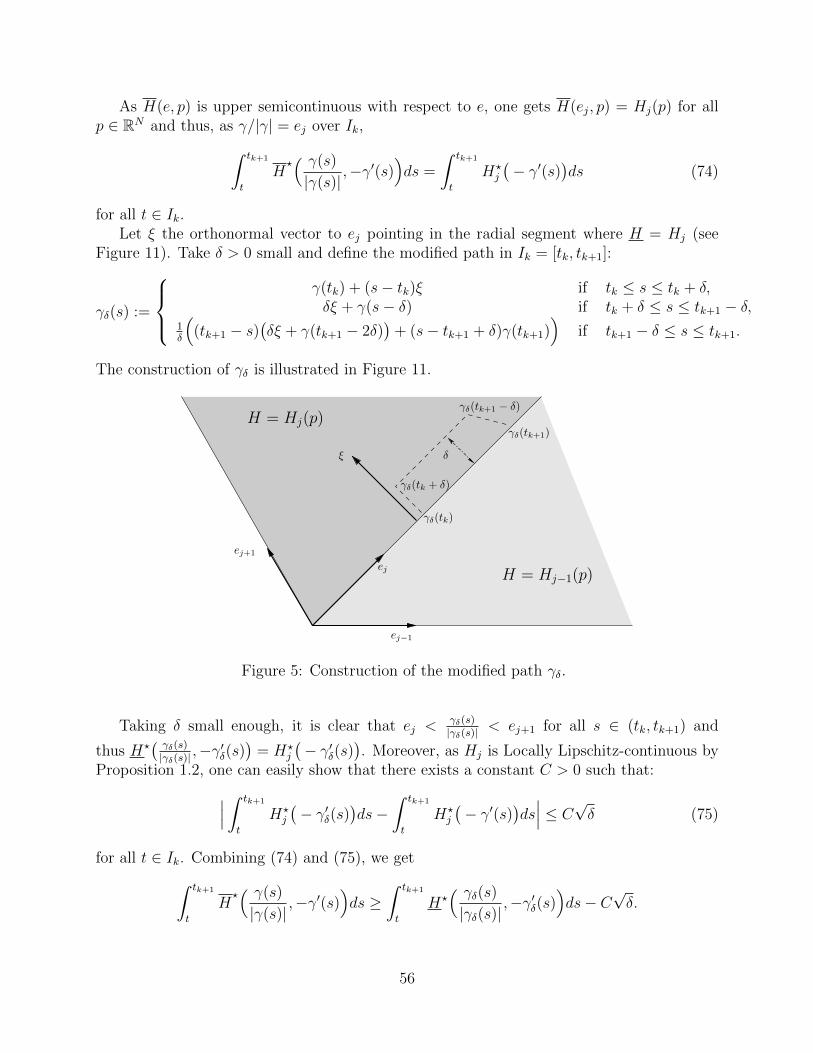
As H(e, p) is upper semicontinuous with respect to e, one gets H(ej, p) = Hj(p) for allp ∈ RN and thus, as γ/|γ| = ej over Ik,∫ tk+1

t

H?( γ(s)

|γ(s)|,−γ′(s)

)ds =

∫ tk+1

t

H?j

(− γ′(s)

)ds (74)

for all t ∈ Ik.Let ξ the orthonormal vector to ej pointing in the radial segment where H = Hj (see

Figure 11). Take δ > 0 small and define the modified path in Ik = [tk, tk+1]:

γδ(s) :=

γ(tk) + (s− tk)ξ if tk ≤ s ≤ tk + δ,δξ + γ(s− δ) if tk + δ ≤ s ≤ tk+1 − δ,

1δ

((tk+1 − s)

(δξ + γ(tk+1 − 2δ)

)+ (s− tk+1 + δ)γ(tk+1)

)if tk+1 − δ ≤ s ≤ tk+1.

The construction of γδ is illustrated in Figure 11.

H = Hj−1(p)

H = Hj(p)

γδ(tk)

ej+1

ej−1

ej

ξ

γδ(tk+1)

γδ(tk+1 − δ)

δ

γδ(tk + δ)

Figure 5: Construction of the modified path γδ.

Taking δ small enough, it is clear that ej <γδ(s)|γδ(s)|

< ej+1 for all s ∈ (tk, tk+1) and

thus H?( γδ(s)|γδ(s)|

,−γ′δ(s))

= H?j

(− γ′δ(s)

). Moreover, as Hj is Locally Lipschitz-continuous by

Proposition 1.2, one can easily show that there exists a constant C > 0 such that:∣∣∣ ∫ tk+1

t

H?j

(− γ′δ(s)

)ds−

∫ tk+1

t

H?j

(− γ′(s)

)ds∣∣∣ ≤ C

√δ (75)

for all t ∈ Ik. Combining (74) and (75), we get∫ tk+1

t

H?( γ(s)

|γ(s)|,−γ′(s)

)ds ≥

∫ tk+1

t

H?( γδ(s)|γδ(s)|

,−γ′δ(s))ds− C

√δ.

56

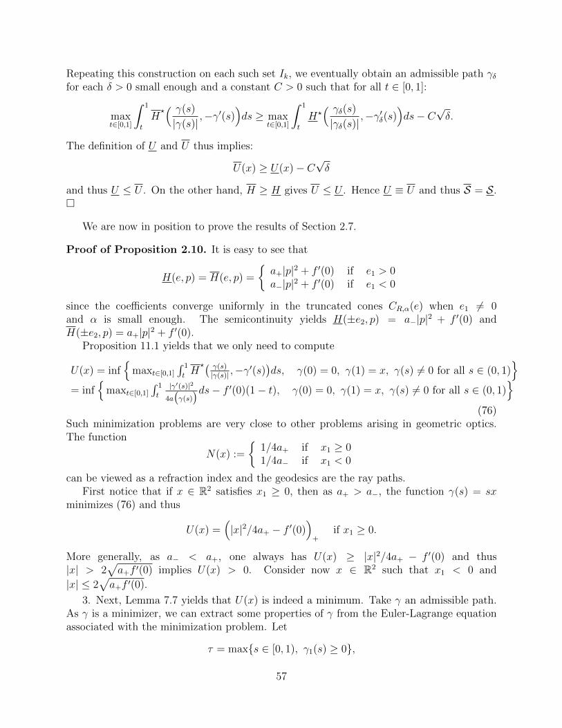
Repeating this construction on each such set Ik, we eventually obtain an admissible path γδfor each δ > 0 small enough and a constant C > 0 such that for all t ∈ [0, 1]:

maxt∈[0,1]

∫ 1

t

H?( γ(s)

|γ(s)|,−γ′(s)

)ds ≥ max

t∈[0,1]

∫ 1

t

H?( γδ(s)|γδ(s)|

,−γ′δ(s))ds− C

√δ.

The definition of U and U thus implies:

U(x) ≥ U(x)− C√δ

and thus U ≤ U . On the other hand, H ≥ H gives U ≤ U . Hence U ≡ U and thus S = S.

We are now in position to prove the results of Section 2.7.

Proof of Proposition 2.10. It is easy to see that

H(e, p) = H(e, p) =

a+|p|2 + f ′(0) if e1 > 0a−|p|2 + f ′(0) if e1 < 0

since the coefficients converge uniformly in the truncated cones CR,α(e) when e1 6= 0and α is small enough. The semicontinuity yields H(±e2, p) = a−|p|2 + f ′(0) andH(±e2, p) = a+|p|2 + f ′(0).

Proposition 11.1 yields that we only need to compute

U(x) = inf

maxt∈[0,1]

∫ 1

tH?( γ(s)|γ(s)| ,−γ

′(s))ds, γ(0) = 0, γ(1) = x, γ(s) 6= 0 for all s ∈ (0, 1)

= inf

maxt∈[0,1]

∫ 1

t|γ′(s)|2

4a(γ(s))ds− f ′(0)(1− t), γ(0) = 0, γ(1) = x, γ(s) 6= 0 for all s ∈ (0, 1)

(76)

Such minimization problems are very close to other problems arising in geometric optics.The function

N(x) :=

1/4a+ if x1 ≥ 01/4a− if x1 < 0

can be viewed as a refraction index and the geodesics are the ray paths.First notice that if x ∈ R2 satisfies x1 ≥ 0, then as a+ > a−, the function γ(s) = sx

minimizes (76) and thus

U(x) =(|x|2/4a+ − f ′(0)

)+

if x1 ≥ 0.

More generally, as a− < a+, one always has U(x) ≥ |x|2/4a+ − f ′(0) and thus|x| > 2

√a+f ′(0) implies U(x) > 0. Consider now x ∈ R2 such that x1 < 0 and

|x| ≤ 2√a+f ′(0).

3. Next, Lemma 7.7 yields that U(x) is indeed a minimum. Take γ an admissible path.As γ is a minimizer, we can extract some properties of γ from the Euler-Lagrange equationassociated with the minimization problem. Let

τ = maxs ∈ [0, 1), γ1(s) ≥ 0,

57

where γ1(s) is the first coordinate of γ(s). As γ is continuous, γ(0) = 0 and γ1(1) = x1 < 0,this maximum is well-defined. One has γ1(τ) = 0 and γ1(s) < 0 for all s ∈ (τ, 1].

Next, assume that τ > 0 and define

γ(s) =

sτγ(τ) if s ∈ [0, τ ],

s−τ1−τ x+ s−τ

1−τ γ(τ) if s ∈ (τ, 1].

One can take γ as a test-function in (76), which gives

U(x) ≤ maxt∈[0,1]

( ∫ 1

tN(γ(s))|γ′(s)|2ds− f ′(0)(1− t)

)= max

0,

|x− γ(τ)|2

4a−(1− τ)− f ′(0)(1− τ),

|γ(τ)|2

4a+τ+|x− γ(τ)|2

4a−(1− τ)− f ′(0)

(77)

On the other hand, the Cauchy-Schwarz inequality yields

|γ(τ)|2 =∣∣∣ ∫ τ

0

γ′(s)ds∣∣∣2 ≤ τ

∫ τ

0

|γ′(s)|2ds and

|x− γ(τ)|2

4a−(1− τ)=

1

4a−(1− τ)

∣∣∣ ∫ 1

τ

γ′∣∣∣2 ≤ 1

4a−

∫ 1

τ

|γ′|2

and these inequalities are equalities if and only if γ′ is constant in (0, τ) and (τ, 1). Hence,the definition of U(x) yields that (77) is smaller than U(x) and thus γ′ is constant in (0, τ)and in (τ, 1).

If τ = 0 then γ(s) = sx and thus U(x) = |x|24a−− f ′(0) in this case.

4. Assume that τ > 0 and let y = γ(τ). We know that y1 = γ1(τ) = 0. We assumethat x2 ≥ 0, the case x2 < 0 can be treated similarly. It is then easy to check that y2 ≥ 0,otherwise ϕ(s) = sx is a better minimizer of (76), which is impossible. Similarly, one canprove that τ > 0 implies x2 6= 0 and y2 6= 0.

For all σ ∈ (0, 1) and z ∈ R, we define

ϕσ,z(s) =

sze2

σif s ∈ [0, σ],

(s− σ)x

(1− σ)+

(1− s)ze2

(1− σ)if s ∈ [σ, 1],

(78)

where e2 is the unit vector associated with the second coordinate axis. We have proved inthe previous step that γ = ϕτ,y2 . But as any function of the form (78) is an appropriatetest-function for the minimization problem (76), we get

U(x) = min

max

0,|x− ze2|2

4a−(1− σ)−f ′(0)(1−σ),

z2

4a+σ+|x− ze2|2

4a−(1− σ)−f ′(0)

, σ ∈ (0, 1), z ∈ R

(79)

and this minimum is reached when σ = τ and z = y2.Take x ∈ R2 such that U(x) > 0. Assume first that |y| < 2

√f ′(0)a+τ . Then

U(x) =|x− y|2

4a−(1− τ)− f ′(0)(1− τ)

58

and z = y2, σ = τ is a local minimizer of

(z, τ) 7→ |x− ze2|2

4a−(1− σ)− f ′(0)(1− σ),

which is a contradiction since this function is increasing with respect to σ. Hence|y| ≥ 2

√f ′(0)a+τ .

Next, assume that |y| = 2√f ′(0)a+τ . Then τ is a minimizer of

σ ∈ (0, 1) 7→|x− 2

√a+f ′(0)σ|2

4a−(1− σ)− f ′(0)(1− σ).

Derivating this function and computing, one obtains:

|x− 2√a+f ′(0)|2 = 4f ′(0)(1− τ)2(a+ − a−),

which gives, after some more computations:

U(x) =

√a+f ′(0)

(x2 − 2

√a+f ′(0)

)4a−

.

This yields a contradiction since x2 < |x| ≤ 2√a+f ′(0) and thus U(x) < 0.

Lastly, if |y| > 2√f ′(0)a+τ , then as (τ, y2) is a critical point for the right-hand side, one

has y2

2

a+τ 2=

|x− y|2

a−(1− τ)2,

y2

a+τ=

x2 − y2

a−(1− τ).

(80)

Taking the square of the second line of (80) and multiplying by a+, one gets

a+(x2 − y2)2 = a−|x− y|2. (81)

In other words, x2 − y2 = r|x1|, where

r :=

√a−

a+ − a−

and, as y2 > 0, one gets x2 > r|x1|. Using the second line of (80) to compute τ , one gets

τ =(

1 +a+

a−× |x1|rx2 − r|x1|

)−1

. (82)

Eventually, a straightforward computation gives

U(x) =y2

2

4a+τ 2− f ′(0) =

1

4a+

(x2 +

|x1|r

)2

− f ′(0).

59

y

0

x2 = rx1

Figure 6: This figure represents the geodesics of the minimization problem (76). The darkerarea corresponds to the case x1 > 0 and the lighter one to the case x1 < 0 and |x1| ≥ r|x2|.The large arrows represent the ray paths in each of these areas.

Similarly, one can prove that if x2 < 0, then −x2 > r|x1| and

U(x) =y2

2

4a+τ− f ′(0) =

1

4a+

(− x2 +

|x1|r

)2

− f ′(0).

5. There only remains to identify the condition τ > 0 in order to conclude. We havealready checked that τ > 0 implies |x2| > r|x1|. On the other hand, if |x2| > r|x1|, thenletting

σ =(

1 +a+

a−× |x1|r|x2| − r|x1|

)−1

and z =

x2 − r|x1| if x2 > 0x2 + r|x1| if x2 < 0

,

the same computations as above gives∫ 1

0

N(ϕσ,z(s))|ϕ′σ,y2(s)|2ds =

1

4a+

(|x2|+

|x1|r

)2.

On the other hand, we know that if τ = 0, then γ(s) = sx and U(x) = |x|24a−− f ′(0). But the

condition x2 > rx1 then yields

U(x)+f ′(0) =|x1|2 + |x2|2

4a−=

1

4a+

( 1

r2+1)|x|2 =

1

4a+

(x2

r−x1

)2

+1

a+

(x2+

x1

r

)2

>1

4a+

(x2+

x1

r

)2.

Hence, γ is not a minimizer of (76), which is a contradiction. We derive a similar contradic-tion if −x2 > r|x1|. We conclude that τ > 0 if and only if |x2| > r|x1|.

Gathering all these facts, we have proved that

U(x) + f ′(0) =

|x|2/4a− if x1 < 0 and |x1| ≤ r|x2|,|x|2/4a+ if x1 ≥ 0,

14a+

(|x2|+ |x1|

r

)2if x1 < 0 and |x1| > r|x2|.

60

Eventually, U(x) = 0 is the equation of two circles of radii 2√a+f ′(0) for x1 ≥ 0 and

2√a−f ′(0) for x1 < 0 and |x1| ≤ r|x2|. For x1 < 0 and x2 > r|x1| or x2 < −r|x1|, it is the

equation of a line, which is the frontier of the convex hull of the two half-circles. This endsthe proof.

Remark: Note that the population leaves the set x1 ≥ 0 with an angle π/2 and enters

x1 < 0 with an angle θ given by tan θ =x2 − y2

|x1|= r =

√a−

a+ − a−, which also reads

sin θ = cos θ × tan θ =tan θ√

1 + tan2 θ=

√a−a+

.

Hence, θ is characterized by 1√a−

sin θ = 1√a+

sin π/2, which is the classical Snell-Descartes law

for geometric optics, with refraction indexes 1√a±

, which is consistent with the local speeds

2√f ′(0)a± in each half-space. It is the first time, as as we know, that such a characterization

is identified in a reaction-diffusion setting.

Proof of Proposition 2.11. As H(e, p) = H(e, p) for all e 6= e2 and p ∈ RN , byProposition 11.1 we only need to characterize the set U > 0, where

U(x) := min maxt∈[0,1]

∫ 1

t

(14|γ′(s)|2 − µ

(γ(s)

))ds, γ ∈ H1([0, 1]), γ(0) = 0, γ(1) = x,

γ(s) 6= 0 for all s ∈ (0, 1),

(83)where µ(x) = µ+ if x1 ≥ 0, µ(x) = µ− if x1 < 0. If x1 ≥ 0, then γ(s) = sx minimizes (83)

and U(x) =( |x|2

4− µ+

)+

. Otherwise, the same arguments as above yield that there exists

a minimizer γ = ϕτ,y2 of (83) defined by (78), with τ ∈ [0, 1)and y = γ(τ), y1 = 0, and themaximum with respect to t ∈ [0, 1] is reached when t = 0, τ or 1.

If τ = 0, then U(x) =( |x|2

4− µ−

)+

. We will now compute U(x) when τ > 0 andcharacterize this situation. Assume that x2 ≥ 0, the case x2 < 0 being treated similarly. Ifx2 = 0, then it is easy to check that γ(s) = sx minimizes (83), which contradicts τ > 0.Putting γ = γσ,z and t = 0, σ or 1 in (83) gives

U(x) = minσ∈(0,1),z∈R

max

0,|x− ze2|2

4(1− σ)− µ−(1− σ),

|z|2

4σ− µ+σ +

|x− ze2|2

4(1− σ)− µ−(1− σ)

where σ = τ and z = y2 minimizes this quantity.

Let x ∈ R2 such that U(x) > 0 and |x| ≤ 2√µ+. Assume first that |y| > 2

√µ+τ . Then

U(x) = minσ∈(0,1),z∈R

( |z|24σ− µ+σ +

|x− ze2|2

4(1− σ)− µ−(1− σ)

)and this minimum is reached when σ = τ and z = y2. As y is a critical point of this functionto minimize, one has:

y2

τ=x2 − y2

1− τ, leading to y2 = τx2.

61

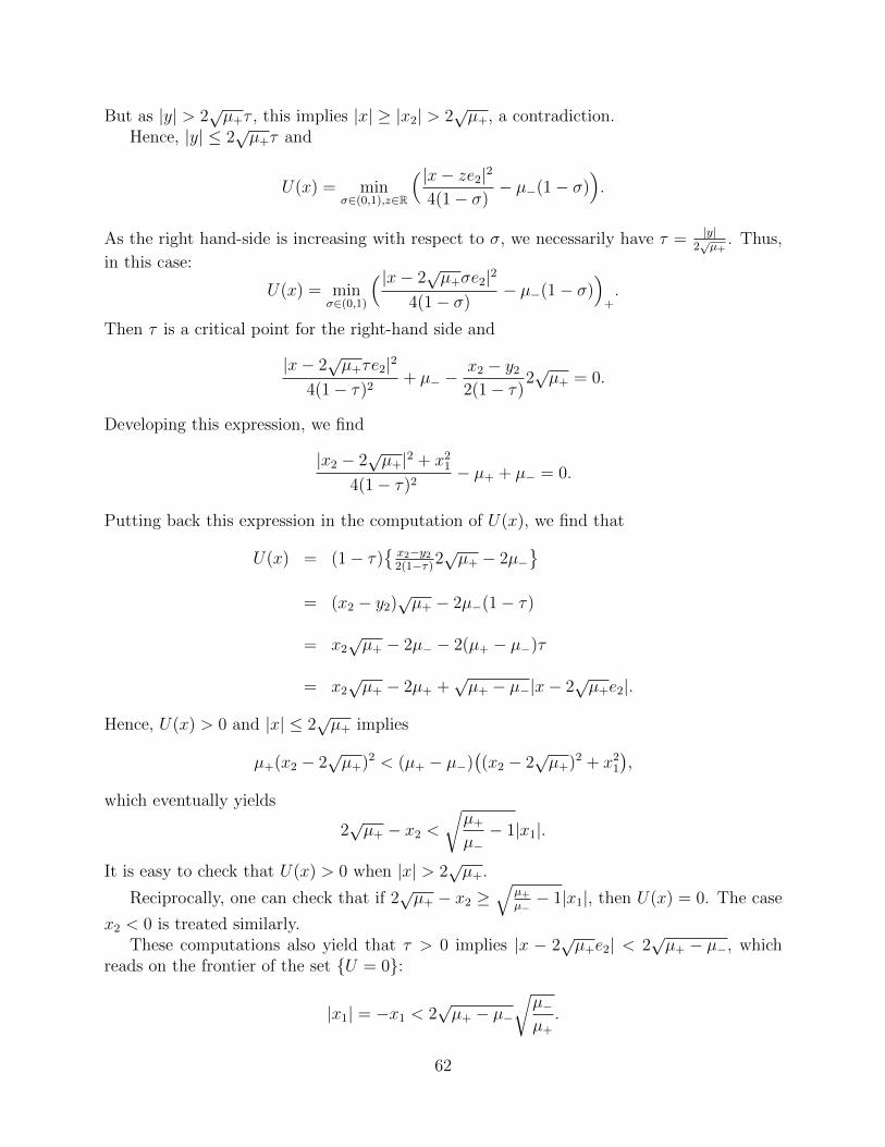
But as |y| > 2√µ+τ , this implies |x| ≥ |x2| > 2

õ+, a contradiction.

Hence, |y| ≤ 2√µ+τ and

U(x) = minσ∈(0,1),z∈R

( |x− ze2|2

4(1− σ)− µ−(1− σ)

).

As the right hand-side is increasing with respect to σ, we necessarily have τ = |y|2√µ+

. Thus,

in this case:

U(x) = minσ∈(0,1)

( |x− 2√µ+σe2|2

4(1− σ)− µ−(1− σ)

)+.

Then τ is a critical point for the right-hand side and

|x− 2√µ+τe2|2

4(1− τ)2+ µ− −

x2 − y2

2(1− τ)2√µ+ = 0.

Developing this expression, we find

|x2 − 2√µ+|2 + x2

1

4(1− τ)2− µ+ + µ− = 0.

Putting back this expression in the computation of U(x), we find that

U(x) = (1− τ)x2−y22(1−τ)

2√µ+ − 2µ−

= (x2 − y2)

√µ+ − 2µ−(1− τ)

= x2√µ+ − 2µ− − 2(µ+ − µ−)τ

= x2√µ+ − 2µ+ +

√µ+ − µ−|x− 2

õ+e2|.

Hence, U(x) > 0 and |x| ≤ 2√µ+ implies

µ+(x2 − 2√µ+)2 < (µ+ − µ−)

((x2 − 2

õ+)2 + x2

1

),

which eventually yields

2√µ+ − x2 <

õ+

µ−− 1|x1|.

It is easy to check that U(x) > 0 when |x| > 2õ+.

Reciprocally, one can check that if 2√µ+ − x2 ≥

√µ+µ−− 1|x1|, then U(x) = 0. The case

x2 < 0 is treated similarly.These computations also yield that τ > 0 implies |x − 2

õ+e2| < 2

√µ+ − µ−, which

reads on the frontier of the set U = 0:

|x1| = −x1 < 2√µ+ − µ−

√µ−µ+

.

62

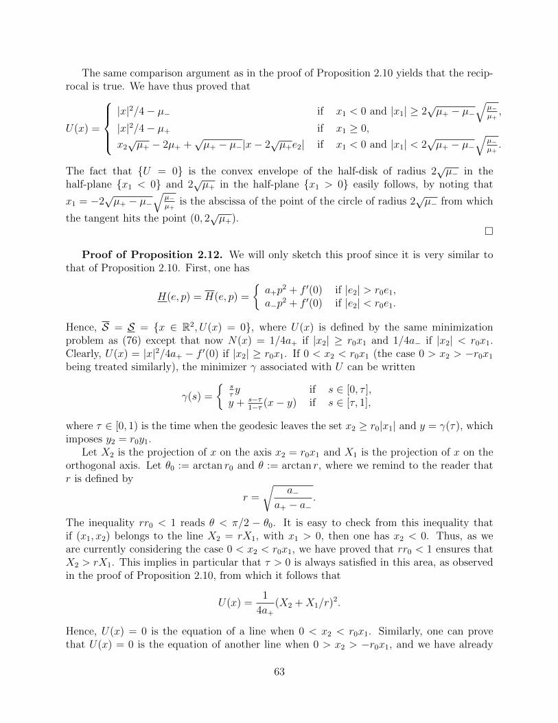
The same comparison argument as in the proof of Proposition 2.10 yields that the recip-rocal is true. We have thus proved that

U(x) =

|x|2/4− µ− if x1 < 0 and |x1| ≥ 2

√µ+ − µ−

√µ−µ+,

|x|2/4− µ+ if x1 ≥ 0,

x2√µ+ − 2µ+ +

√µ+ − µ−|x− 2

õ+e2| if x1 < 0 and |x1| < 2

√µ+ − µ−

√µ−µ+.

The fact that U = 0 is the convex envelope of the half-disk of radius 2√µ− in the

half-plane x1 < 0 and 2õ+ in the half-plane x1 > 0 easily follows, by noting that

x1 = −2√µ+ − µ−

√µ−µ+

is the abscissa of the point of the circle of radius 2√µ− from which

the tangent hits the point (0, 2õ+).

Proof of Proposition 2.12. We will only sketch this proof since it is very similar tothat of Proposition 2.10. First, one has

H(e, p) = H(e, p) =

a+p

2 + f ′(0) if |e2| > r0e1,a−p

2 + f ′(0) if |e2| < r0e1.

Hence, S = S = x ∈ R2, U(x) = 0, where U(x) is defined by the same minimizationproblem as (76) except that now N(x) = 1/4a+ if |x2| ≥ r0x1 and 1/4a− if |x2| < r0x1.Clearly, U(x) = |x|2/4a+ − f ′(0) if |x2| ≥ r0x1. If 0 < x2 < r0x1 (the case 0 > x2 > −r0x1

being treated similarly), the minimizer γ associated with U can be written

γ(s) =

sτy if s ∈ [0, τ ],y + s−τ

1−τ (x− y) if s ∈ [τ, 1],

where τ ∈ [0, 1) is the time when the geodesic leaves the set x2 ≥ r0|x1| and y = γ(τ), whichimposes y2 = r0y1.

Let X2 is the projection of x on the axis x2 = r0x1 and X1 is the projection of x on theorthogonal axis. Let θ0 := arctan r0 and θ := arctan r, where we remind to the reader thatr is defined by

r =

√a−

a+ − a−.

The inequality rr0 < 1 reads θ < π/2 − θ0. It is easy to check from this inequality thatif (x1, x2) belongs to the line X2 = rX1, with x1 > 0, then one has x2 < 0. Thus, as weare currently considering the case 0 < x2 < r0x1, we have proved that rr0 < 1 ensures thatX2 > rX1. This implies in particular that τ > 0 is always satisfied in this area, as observedin the proof of Proposition 2.10, from which it follows that

U(x) =1

4a+

(X2 +X1/r)2.

Hence, U(x) = 0 is the equation of a line when 0 < x2 < r0x1. Similarly, one can provethat U(x) = 0 is the equation of another line when 0 > x2 > −r0x1, and we have already

63

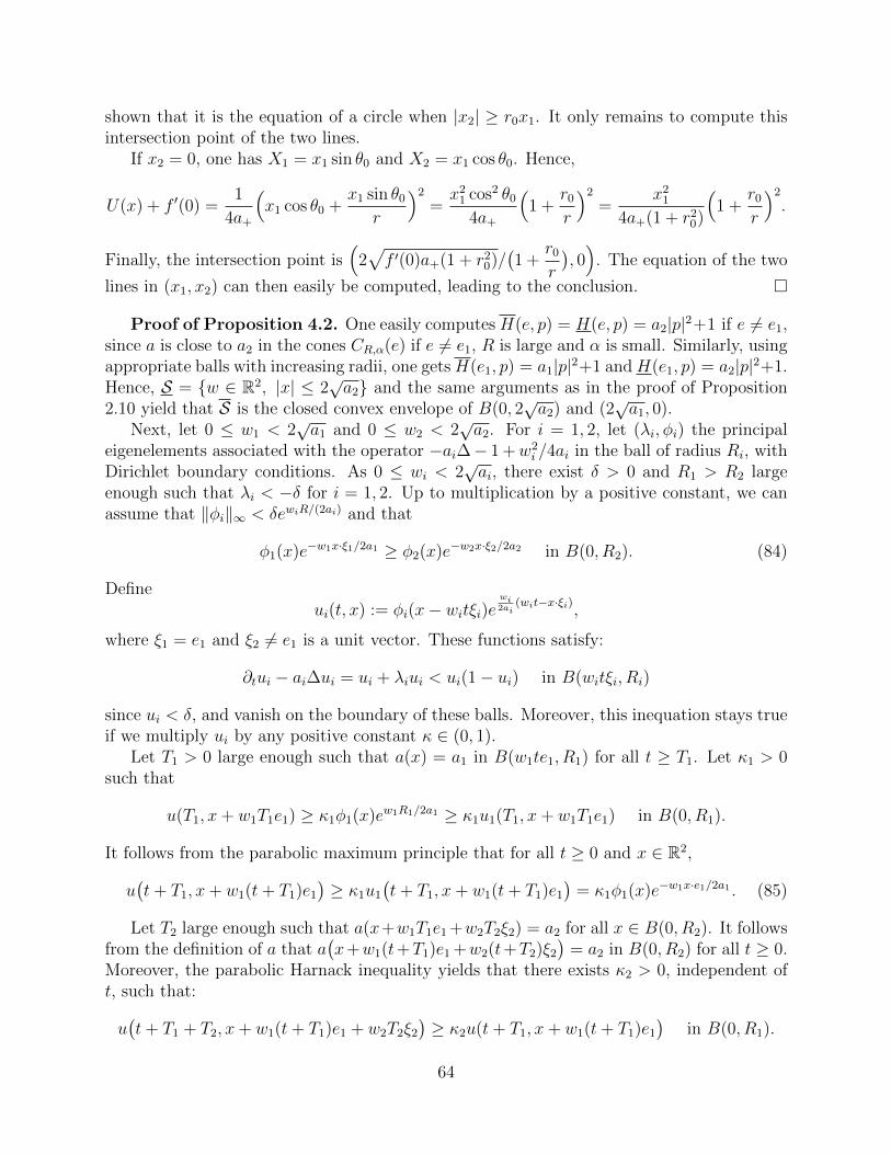
shown that it is the equation of a circle when |x2| ≥ r0x1. It only remains to compute thisintersection point of the two lines.

If x2 = 0, one has X1 = x1 sin θ0 and X2 = x1 cos θ0. Hence,

U(x) + f ′(0) =1

4a+

(x1 cos θ0 +

x1 sin θ0

r

)2

=x2

1 cos2 θ0

4a+

(1 +

r0

r

)2

=x2

1

4a+(1 + r20)

(1 +

r0

r

)2

.

Finally, the intersection point is(

2√f ′(0)a+(1 + r2

0)/(1 +

r0

r

), 0)

. The equation of the two

lines in (x1, x2) can then easily be computed, leading to the conclusion.

Proof of Proposition 4.2. One easily computes H(e, p) = H(e, p) = a2|p|2+1 if e 6= e1,since a is close to a2 in the cones CR,α(e) if e 6= e1, R is large and α is small. Similarly, usingappropriate balls with increasing radii, one gets H(e1, p) = a1|p|2+1 and H(e1, p) = a2|p|2+1.Hence, S = w ∈ R2, |x| ≤ 2

√a2 and the same arguments as in the proof of Proposition

2.10 yield that S is the closed convex envelope of B(0, 2√a2) and (2

√a1, 0).

Next, let 0 ≤ w1 < 2√a1 and 0 ≤ w2 < 2

√a2. For i = 1, 2, let (λi, φi) the principal

eigenelements associated with the operator −ai∆− 1 +w2i /4ai in the ball of radius Ri, with

Dirichlet boundary conditions. As 0 ≤ wi < 2√ai, there exist δ > 0 and R1 > R2 large

enough such that λi < −δ for i = 1, 2. Up to multiplication by a positive constant, we canassume that ‖φi‖∞ < δewiR/(2ai) and that

φ1(x)e−w1x·ξ1/2a1 ≥ φ2(x)e−w2x·ξ2/2a2 in B(0, R2). (84)

Defineui(t, x) := φi(x− witξi)e

wi2ai

(wit−x·ξi),

where ξ1 = e1 and ξ2 6= e1 is a unit vector. These functions satisfy:

∂tui − ai∆ui = ui + λiui < ui(1− ui) in B(witξi, Ri)

since ui < δ, and vanish on the boundary of these balls. Moreover, this inequation stays trueif we multiply ui by any positive constant κ ∈ (0, 1).

Let T1 > 0 large enough such that a(x) = a1 in B(w1te1, R1) for all t ≥ T1. Let κ1 > 0such that

u(T1, x+ w1T1e1) ≥ κ1φ1(x)ew1R1/2a1 ≥ κ1u1(T1, x+ w1T1e1) in B(0, R1).

It follows from the parabolic maximum principle that for all t ≥ 0 and x ∈ R2,

u(t+ T1, x+ w1(t+ T1)e1

)≥ κ1u1

(t+ T1, x+ w1(t+ T1)e1

)= κ1φ1(x)e−w1x·e1/2a1 . (85)

Let T2 large enough such that a(x+w1T1e1 +w2T2ξ2) = a2 for all x ∈ B(0, R2). It followsfrom the definition of a that a

(x+w1(t+T1)e1 +w2(t+T2)ξ2

)= a2 in B(0, R2) for all t ≥ 0.

Moreover, the parabolic Harnack inequality yields that there exists κ2 > 0, independent oft, such that:

u(t+ T1 + T2, x+ w1(t+ T1)e1 + w2T2ξ2

)≥ κ2u(t+ T1, x+ w1(t+ T1)e1

)in B(0, R1).

64

This implies

u(t+ T1 + T2, x+ w1(t+ T1)e1 + w2T2ξ2

)≥ κ1κ2φ1(x)e−w1x·e1/2a1 ≥ κ1κ2u2(T2, x+ w2T2ξ2

),

by (84). The parabolic maximum principle gives, for all s ≥ 0, t ≥ 0:

u(s+ t+ T1 + T2, x+ w1(t+ T1)e1 + w2(s+ T2)ξ2

)≥ κ1κ2u2(s+ T2, x+ w2(s+ T2)ξ2

)= κ1κ2φ2(x)e

− wi2ai

x·ξi .(86)

Consider now a given w in the interior of the closed convex envelope of B(0, 2√a2) and

(2√a1, 0). We could write w = (1− τ)w1e1 + τw2ξ2, where τ ∈ (0, 1), w1 ∈ [0, 2√a1) and

w2ξ2 ∈ B(0, 2√a2), that is, 0 ≤ w2 < 2

√a2 and |ξ2| = 1.

We now apply the above results. First, if ξ2 = e1, then inequality (85) immediatelyimplies

lim inft→+∞

u(t, (1− τ)w1e1t+ τw2e1t

)= lim inf

t→+∞u(t, tw) ≥ κ1φ1(0) > 0.

Next, if ξ2 6= e1, replacing t + T1 by (1− τ)t and s + T2 by τt in (86), which is possible if tis large enough since τ ∈ (0, 1), one gets

u(t, (1− τ)w1e1t+ τw2ξ2t

)= u(t, tw) ≥ κ1κ2φ2(0).

Moreover, the reader could check that these estimates hold locally uniformly with respect toτ, ξ2, w1, w2, that is, locally uniformly with respect to w. It follows that

lim inft→+∞

u(t, tw) > 0,

and thus our hypotheses on f (6) and classical arguments (see for example Theorem 1.6 andProposition 1.8 of [12]) yield

lim inft→+∞

u(t, tw

)= 1.

Moreover, as this convergence is locally uniform around any w in the interior of the closedconvex envelope of B(0, 2

√a2) and (2√a1, 0), it is also uniform in any of its compact

subset, which concludes the proof.

References

[1] O. Alvarez, J.-M. Lasry, P.-L. Lions. Convex viscosity solutions and state constraints. J.Math. Pures Appl., 76(3):265?288, 1997.

[2] S. Armstrong, and P. E. Souganidis. Stochastic homogenization of Hamilton-Jacobiand degenerate Bellman equations in unbounded environments. J. Math. Pures Appl.97(5):460-504, 2012.

[3] S. Armstrong, and H. V. Tran. Viscosity solutions of general viscous Hamilton-Jacobiequations. Math. Ann., 361(3-4):647–687, 2015.

65

[4] D.G. Aronson, and H.F. Weinberger. Multidimensional nonlinear diffusions arising inpopulation genetics. Adv. Math., 30:33–76, 1978.

[5] G Barles, and E. Chasseigne. (Almost) Everything You Always Wanted to Know AboutDeterministic Control Problems in Stratified Domains, preprint, 2015.

[6] G. Barles, and B. Perthame. Exit time problems in optimal control and vanishing vis-cosity method. SIAM J. Control Optim., 26(5):1133–1148, 1988.

[7] G. Barles, and B. Perthame. Discontinuous solutions of deterministic optimal stoppingtime problems. RAIRO Model. Math. Anal. Numer., 21(4):557–579, 1987.

[8] H. Berestycki, and F. Hamel. Front propagation in periodic excitable media. Comm.Pure Appl. Math., 55:949–1032, 2002.

[9] H. Berestycki, and F. Hamel. Generalized travelling waves for reaction-diffusion equa-tions. Perspectives in Nonlinear Partial Differential Equations. In honor of H. Brezis,Contemp. Math. 446, Amer. Math. Soc., pages 101–123, 2007.

[10] H. Berestycki, and F. Hamel. Generalized transition waves and their properties. Com-munications on Pure and Applied Mathematics, 65(5):592–648, 2012.

[11] H. Berestycki, F. Hamel, and H. Matano. Bistable travelling waves around an obstacle.Comm. Pure Appl. Math., 62:729-788, 2009.

[12] H. Berestycki, F. Hamel, and G. Nadin. Asymptotic spreading in heterogeneous diffusiveexcitable media. J. Func. Anal., 255(9):2146–2189, 2008.

[13] H. Berestycki, F. Hamel, and N. Nadirashvili. Propagation speed for reaction-diffusionequations in general domains. C.R. Acad. Sci. Paris Ser. I, 339:163–168, 2004.

[14] H. Berestycki, F. Hamel, and N. Nadirashvili. The speed of propagation for KPP typeproblems. I - Periodic framework. J. European Math. Soc. 7:173–213, 2005.

[15] H. Berestycki, F. Hamel, and N. Nadirashvili. The speed of propagation for KPP typeproblems. II - General domains. J. Amer. Math. Soc. 23:1-34, 2010.

[16] H. Berestycki, F. Hamel, and L.Roques. Analysis of the periodically fragmented envi-ronment model : II - biological invasions and pulsating travelling fronts. J. Math. PuresAppl., 84:1101–1146, 2005.

[17] H. Berestycki, F. Hamel, and L. Rossi. Liouville-type results for semilinear ellipticequations in unbounded domains. Ann. Mat. Pura Appl., 186 (4):469–507, 2007.

[18] H. Berestycki, and G. Nadin. Spreading speeds for one-dimensional monostable reaction-diffusion equations. J. Math. Phys., 53(11), 2012.

[19] H. Berestycki, L. Nirenberg, and S. R. S. Varadhan. The principal eigenvalue andmaximum principle for second order elliptic operators in general domains. Comm. PureAppl. Math., 47:47–92, 1994.

66

[20] H. Berestycki, J.-M. Roquejoffre, and L. Rossi. The shape of expansion induced by aline with fast diffusion in Fisher-KPP equations, em preprint.

[21] H. Berestycki, and L. Rossi. On the principal eigenvalue of elliptic operators in RN andapplications. J. European Math. Soc., 8:195–215, 2006.

[22] H. Berestycki, and L. Rossi. Generalizations and properties of the principal eigenvalueof elliptic operators in unbounded domains preprint.

[23] S. Bochner. Beitrage zur theorie der fastperiodischen funktionen. Math. Ann., 96:119–147, 1926.

[24] M. G. Crandall, H. Ishii and P.-L. Lions. User’s guide to viscosity solutions of secondorder partial differential equations. Bull. Amer. Math. Soc., 27:1–67, 1992.

[25] M. G. Crandall, and P.-L. Lions. Viscosity Solutions of Hamilton-Jacobi Equations.Trans. Amer. Math. Soc., 277(1):1–42, 1983.

[26] A. Davini, and A. Siconolfi. Exact and approximate correctors for stochastic Hamilto-nians: the 1–dimensional case. Math. Annal., 345(4):749–782, 2009.

[27] L.C. Evans. Periodic homogenization of certain fully nonlinear partial differential equa-tions. Proc. Roy. Soc. Edinburgh Sect. A, 120:245–265, 1992.

[28] L. C. Evans, and P. E. Souganidis. A PDE approach to geometric optics for certainsemilinear parabolic equations. Indiana Univ. Math., 38(1):141–172, 1989.

[29] J. Fang, and X.-Q. Zhao. Bistable Traveling Waves for Monotone Semiflows with Ap-plications. Journal of European Math. Soc., in press.

[30] R. A. Fisher. The advance of advantageous genes. Ann. Eugenics, 7:335–369, 1937.

[31] M. Freidlin. Limit Theorems for Large Deviations and Reaction-Diffusion Equations.Ann. Probab., 13(3):639–675, 1985.

[32] M. Freidlin. On wave front propagation in periodic media. In: Stochastic analysis andapplications, ed. M. Pinsky, Advances in Probability and related topics, 7:147–166, 1984.

[33] M. Freidlin, and J. Gartner. On the propagation of concentration waves in periodic andrandom media. Sov. Math. Dokl., 20:1282–1286, 1979

[34] M. Freidlin, and T.-Y. Lee. Wave front propagation and large deviations for diffusion-transmutation process. Probab. Theory Relat. Fields, 106:39–70, 1996.

[35] J. Garnier, T. Giletti, and G. Nadin. Maximal and minimal spreading speeds for re-action diffusion equations in nonperiodic slowly varying media. J. Dynam. DifferentialEquations, 24(3):521–538, 2012.

[36] Y. Giga, P. Gorka, and P. Rybka. A comparison principle for Hamilton-Jacobi equationswith discontinuous Hamiltonians. Proc. Amer. Math. Soc., 139(5):1777–1785, 2011.

67

[37] C. Imbert. Convexity of solutions and C1,1 estimates for fully nonlinear elliptic equa-tions. J. Math. Pures et Appl., 85(6):791–807, 2006.

[38] C. Imbert, and R. Monneau. Flux-limited solutions for quasi-convex Hamilton-Jacobiequations on networks. Preprint, 2014.

[39] C. Imbert, and R. Monneau. Quasi-convex Hamilton-Jacobi equations posed on junc-tions: the multi-dimensional case. Preprint, 2014.

[40] H. Ishii. Hamilton-Jacobi equations with discontinuous Hamiltonians on arbitrary opensets, Bull. Fac. Sci. Engrg. Chuo Univ., 28:33–77, 1985.

[41] H. Ishii. Perron’s method for Hamilton-Jacobi equations, Duke Math. J., 55(2):369–384,1987.

[42] H. Ishii. A boundary value problem of the Dirichlet type for Hamilton-Jacobi equations.Ann. Scuola Norm. Sup. Pisa Cl. Sci., 16(1):105–135, 1989.

[43] H. Ishii. Homogenization of the Cauchy problem for Hamilton-Jacobi equations. Stochas-tic analysis, control, optimization and applications, 305–324, Systems Control Found.Appl., Birkhauuser Boston, Boston, MA, 1999.

[44] A.N. Kolmogorov, I.G. Petrovsky, and N.S. Piskunov. Etude de l equation de la diffusionavec croissance de la quantite de matiere et son application a un probleme biologique.Bulletin Universite d’Etat a Moscou (Bjul. Moskowskogo Gos. Univ.), 1–26, 1937.

[45] L. Kong, and W. Shen. Positive Stationary Solutions and Spreading Speeds of KPPEquations in Locally Spatially Inhomogeneous Media. Methods and Applications of Anal-ysis, 18:427-456, 2011.

[46] E. Kosygina, F. Rezakhanlou and S.R.S. Varadhan. Stochastic homogenization ofHamilton-Jacobi-Bellman Equations. Communications on Pure and Applied Mathemat-ics, 59(10):1489–1521, 2006.

[47] E. Kosygina, and S.R.S. Varadhan. Homogenization of Hamilton-Jacobi-Bellman equa-tions with respect to time-space shifts in a stationary ergodic medium. Communicationson Pure and Applied Mathematics, 61(6):816–847, 2008.

[48] B.M. Levitan. Almost periodic functions and differential equations. Cambridge Univer-sity Press, 1982.

[49] B. Lewin, and B. Lewitan. On the Fourier series of generalized almost periodic functions.Comptes-rendus (Doklady) de l’Academie des Sciences de l’URSS, 22(9):539–542, 1939.

[50] P.-L. Lions, and P. E. Souganidis. Correctors for the homogenization theory of Hamilton-Jacobi equations. Comm Pure Applied Math., LVI:1501–1524, 2003.

68

[51] P.-L. Lions, and P. E. Souganidis. Homogenization of degenerate second-order PDEin periodic and almost periodic environments and applications. Ann. Inst. H. Poincare,Anal. Non Lineaire, 22(5):667-677, 2005.

[52] P.-L. Lions, and P. E. Souganidis. Homogenization of “viscous” Hamilton-Jacobi equa-tions in stationary ergodic media. Comm. Partial Differential Equations, 30(1-3):335–375,2005.

[53] R.-L. Lions, and P. E. Souganidis. Stochastic homogenization of Hamilton-Jacobiand ”viscous”-Hamilton-Jacobi equations with convex nonlinearities?revisited. Commun.Math. Sci. 8(2):627–637, 2010.

[54] A. J. Majda, and P. E. Souganidis. Large-scale front dynamics for turbulent reaction-diffusion equations with separated velocity scales. Nonlinearity, 7(1):1–30, 1994.

[55] H. Matano. Traveling waves in spatially random media. RIMS Kokyuroku, 1337:1–9,2003.

[56] H. Matano, and M. Nara. Large time behavior of disturbed planar fronts in the Allen-Cahn equation. J. Differential Equations, 251(12): 3522–3557, 2011.

[57] A. Mellet, J. Nolen, J.-M. Roquejoffre, and L. Ryzhik. Stability of generalized transitionsfronts. Comm. Partial Differential Equations, 34:521–552, 2009.

[58] A. Mellet, J.-M. Roquejoffre, and Y. Sire. Generalized fronts for one-dimensionnalreaction-diffusion equations. Discrete Contin. Dyn. Syst., 26(1):303–312, 2009.

[59] G. Nadin. Traveling fronts in space-time periodic media. J. Math. Pures Appl., 92:232–262, 2009.

[60] G. Nadin, and L. Rossi. Propagation phenomena for time heterogeneous KPP reaction-diffusion equations. J. Math. Pures Appl. (9), 98(6):633–653, 2012.

[61] J. Nolen, J.-M. Roquejoffre, L. Ryzhik and A. Zlatos. Existence and non-existence ofFisher-KPP transition fronts. Archive for Rational Mechanics and Analysis, 203(1):217–246, 2012.

[62] J. Nolen, M. Rudd, and J. Xin. Existence of KPP fronts in spatially-temporally periodicadvection and variational principle for propagation speeds. Dynamics of PDE, 2(1):1–24,2005.

[63] J. Nolen, and L. Ryzhik. Traveling waves in a one-dimensional heterogeneous medium.Ann. Inst. H. Poincare Anal. Non Lineaire, 26(3):1021–1047, 2009.

[64] J. Nolen, and J. Xin. Asymptotic Spreading of KPP Reactive Fronts in IncompressibleSpace-Time Random Flows. Ann. de l’Inst. Henri Poincare – Analyse Non Lineaire,26(3):815–839, 2008.

69

[65] J. Nolen, and J. Xin. KPP Fronts in 1D Random Drift. Discrete and ContinuousDynamical Systems B, 11(2), 2009

[66] J. Nolen, and J. Xin. Variational Principle of KPP Front Speeds in Temporally RandomShear Flows with Applications. Communications in Mathematical Physics, 269:493–532,2007.

[67] G. C. Papanicolaou, and S.R.S. Varadhan. Boundary value problems with rapidlyoscillating random coefficients. Proceedings of Conference on Random Fields, Eszter-gom, Hungary, 1979, published in Seria Colloquia Mathematica Societatis Janos Bolyai,27:835–873, North Holland, 1981.

[68] E. A. Robinson. The dynamical properties of Penrose tilings. Trans AMS, 348:4447–4464, 1996.

[69] L. Rossi. Liouville type results for periodic and almost periodic linear operators. Ann.I. H. Poincar AN, 26:24812502, 2009.

[70] R. Schwab. Stochastic Homogenization of Hamilton-Jacobi Equations in StationaryErgodic Spatio-Temporal Media. to appear in Indiana Univ. Math. J..

[71] W. Shen. Travelling waves in time almost periodic structures governed by bistablenonlinearities. I. Stability and uniqueness. J. Differential Equations, 159(1):1–54, 1999.

[72] W. Shen. Travelling waves in time almost periodic structures governed by bistablenonlinearities. II. Existence. J. Differential Equations, 159(1):55–101, 1999.

[73] W. Shen. Traveling waves in diffusive random media. J. Dynam. Differential Equations,16(4):1011–1060, 2004.

[74] W. Shen. Traveling waves in time dependent bistable equations. Differential IntegralEquations, 19(3):241–278, 2006.

[75] W. Shen. Variational principle for spatial spreading speeds and generalized propagatingspeeds in time almost periodic and space periodic KPP models. to appear in Trans. ofthe AMS, 2009.

[76] W. Shen. Existence, uniqueness, and stability of generalized traveling waves in timedependent monostable equations. J. Dynam. Differential Equations, 23(1):1–44, 2011.

[77] P. Soravia. Boundary value problems for Hamilton-Jacobi equations with discontinuousLagrangian. Indiana Univ. Math. J., 51(2):451–477, 2002.

[78] P. E. Souganidis. Stochastic homogenization of Hamilton-Jacobi equations and someapplications. Asymptot. Anal., 20 (1):1–11, 1999.

[79] A. Tourin. A comparison theorem for a piecewise Lipschitz continuous Hamiltonianand application to Shape-from-Shading problems. Numerische Mathematik, 62(1):75–85,1992.

70

[80] W. A. Veech. On a Theorem of Bochner. Ann. Math., 86, 1967.

[81] H. Weinberger. On spreading speed and travelling waves for growth and migrationmodels in a periodic habitat. J. Math. Biol., 45:511–548, 2002.

[82] G. Wulff. Zur Frage der Geschwindigkeit des Wachstums und der Auflosung der Krys-tallflagen. Z. Kryst. Mineral, 34:449, 1901.

[83] J. Xin. Front propagation in heterogeneous media. SIAM Rev., 42:161–230, 2000.

[84] A. Zlatos. Transition fronts in inhomogeneous Fisher-KPP reaction-diffusion equations.J. Math. Pures Appl., 98:89–102, 2012.

[85] A. Zlatos. Generalized traveling waves in disordered media: existence, uniqueness, andstability. Arch. Ration. Mech. Anal., 208(2):447–480, 2013.

[86] A. Zlatos. Propagation of reactions in inhomogeneous media, preprint.

71