Embed Size (px)
Citation preview

Asymptotic Convergence Properties of EM-Type
Algorithms
1
Alfred O. Hero
�
and Je�rey A. Fessler
��
�
Dept. of Electrical Engineering and Computer Science and
��
Division of Nuclear Medicine
The University of Michigan, Ann Arbor, MI 48109
ABSTRACT
We analyze the asymptotic convergence properties of a general class of EM-type algorithms for es-
timating an unknown parameter via alternating estimation and maximization. As examples, this
class includes ML-EM, penalized ML-EM, Green's OSL-EM, and many other approximate EM al-
gorithms. A theorem is given which provides conditions for monotone convergence with respect
to a given norm and speci�es an asymptotic rate of convergence for an algorithm in this class.
By investigating di�erent parameterizations, the condition for monotone convergence can be used
to establish norms under which the distance between successive iterates and the limit point of the
EM-type algorithm approaches zero monotonically. We apply these results to a modi�ed ML-EM
algorithm with stochastic complete/incomplete data mapping and establish global monotone conver-
gence for a linear Gaussian observation model. We then establish that in the �nal iterations the
unpenalized and quadratically penalized ML-EM algorithms for PET image reconstruction converge
monotonically relative to two di�erent norms on the logarithm of the images.
I. INTRODUCTION
The maximum-likelihood (ML) expectation-maximization (EM) algorithm is a popular iterative
method for �nding the maximum likelihood estimate
^
� of a parameter � when the likelihood func-
tion is too di�cult to maximize directly [4, 23, 17, 18, 19, 5, 22]. The penalized ML-EM algorithm
is a variant of the ML-EM algorithm which can be used for �nding MAP estimates of a random
parameter [10, 11, 12]. To apply the penalized or unpenalized ML-EM algorithm requires formu-
lation of the estimation problem in terms of the actual data sample, called the incomplete data,
and a hypothetical data set, called the complete data. To be able to easily implement the ML-EM
algorithm the complete data must be chosen in such a way that: the complete data log-likelihood
function is easily estimated from the incomplete data via conditional expectation (E); and the com-
plete data log-likelihood function is easily maximized (M). Three types of convergence results are
of practical importance: conditions under which the sequence of estimates converges globally to a
1
This research was supported in part by the National Science Foundation under grant BCS-9024370 and a DOE
Alexander Hollaender Postdoctoral Fellowship.
1

�xed point, norms under which the convergence is monotone; and the asymptotic convergence rate
of the algorithm. A number of authors [24, 16, 3] have derived global convergence results for a wide
range of exact ML-EM algorithms by using an information divergence approach. These authors
establish monotone convergence of ML-EM algorithms in the information divergence measure. This
guarantees that successive iterates of the EM algorithm monotonically increase likelihood. While
increasing likelihood is an attractive property, it does not guarantee monotone convergence in terms
of Cauchy convergence: successive iterates of the EM algorithm reduce the distance to the ML esti-
mate in some norm. In addition, for some implementations the region of convergence may only be a
small subset of the entire parameter space so that global convergence may not hold. Furthermore,
in some cases the ML-EM algorithm can only be implemented by making simplifying approxima-
tions in the conditional expectation step (E) or the maximization step (M). While these algorithms
have an alternating estimation-maximization structure similar to the exact ML-EM algorithm, the
information divergence approach developed to establish global convergence of the exact ML-EM
algorithm may not be e�ective. In this paper we develop a generally applicable approach to conver-
gence analysis which allows us to study monotone convergence and asymptotic convergence rates
for algorithms which can be implemented via alternating estimation-maximization.
We de�ne an EM-type algorithm as any iterative algorithm of the form �
i+1
= argmax
�
Q(�; �
i
),
i = 1; 2; : : : where � 2 � � IR
p
. This general iterative algorithm specializes to popular EM-type
algorithms including: penalized and penalized ML-EM algorithms [4, 11], generalized ML-EM
with stochastic complete-incomplete data mapping [6], one-step-late (OSL) penalized ML-EM [9],
majorization methods [?], and approximate ML-EM algorithms such as the linear and quadratic
approximations introduced in [2, 1]. Let �
�
be a �xed point of the EM-type algorithm which occurs
on the interior of � and assume that Q is a smooth function of both arguments. We give an
implicit relation between successive di�erences ��
i+1
def
= �
i+1
� �
�
and ��
i
def
= �
i
� �
�
of the form
��
i+1
= M
�1
1
M
2
��
i+1
where M
1
and M
2
are p � p matrices associated with the 2p � 2p Hessian
matrix of Q(�
i+1
; �
i
). Using this implicit relation we derive conditions for monotone convergence
and show that the asymptotic rate of convergence is the maximum magnitude eigenvalue of the
curvature matrix [r
20
Q(�
�
; �
�
)]
�1
r
11
Q(�
�
; �
�
) where r
20
Q and r
11
Q are p � p matrices of mixed
derivatives at the point (�
�
; �
�
). For ML-EM this curvature matrix is monotonically increasing in
the conditional Fisher information matrix associated with the complete data.
We provide several illustrations of our convergence results. First we consider a generalized
version of the standard ML-EM algorithm which permits the complete data to be speci�ed in such
a way that it is related to the incomplete data via a possibly random transformation. This algorithm
is of interest since the conventional convergence analysis of the EM algorithm is inapplicable due to
the presence of additive noise in the mapping from the complete data to the incomplete data. Then
we give general forms for the asymptotic convergence rates for the linearized EM algorithm [2], the
unpenalized and penalized ML-EM algorithms, the OSL penalized ML-EM algorithm [9], and the
majorization method [?]. For the latter algorithms the asymptotic convergence rates are of similar
form to those obtained by Green [9] for the standard case of deterministic complete/incomplete
data mapping. Afterwards we consider ML-EM and penalized ML-EM for two important practical
2
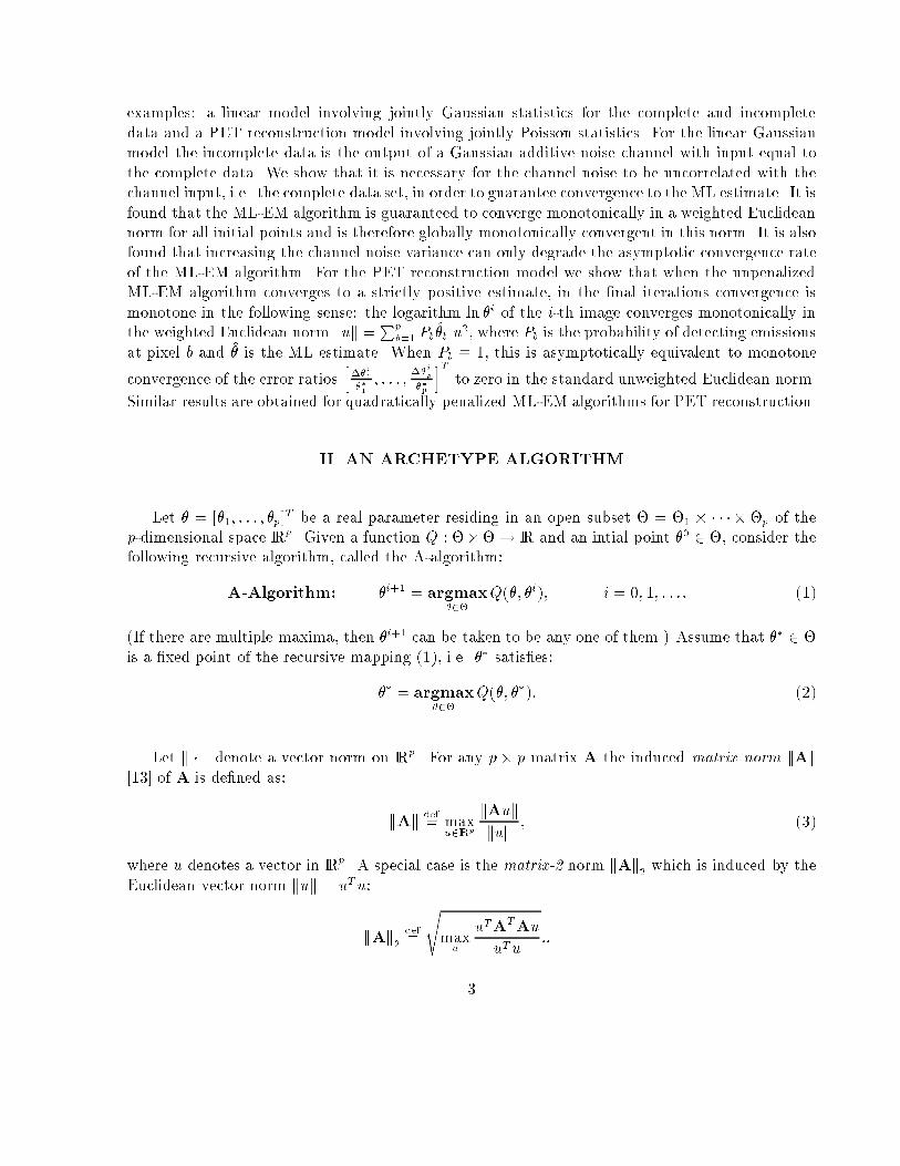
examples: a linear model involving jointly Gaussian statistics for the complete and incomplete
data and a PET reconstruction model involving jointly Poisson statistics. For the linear Gaussian
model the incomplete data is the output of a Gaussian additive noise channel with input equal to
the complete data. We show that it is necessary for the channel noise to be uncorrelated with the
channel input, i.e. the complete data set, in order to guarantee convergence to the ML estimate. It is
found that the ML-EM algorithm is guaranteed to converge monotonically in a weighted Euclidean
norm for all initial points and is therefore globally monotonically convergent in this norm. It is also
found that increasing the channel noise variance can only degrade the asymptotic convergence rate
of the ML-EM algorithm. For the PET reconstruction model we show that when the unpenalized
ML-EM algorithm converges to a strictly positive estimate, in the �nal iterations convergence is
monotone in the following sense: the logarithm ln �
i
of the i-th image converges monotonically in
the weighted Euclidean norm kuk =
P
p
b=1
P
b
^
�
b
u
2
, where P
b
is the probability of detecting emissions
at pixel b and
^
� is the ML estimate. When P
b
� 1, this is asymptotically equivalent to monotone
convergence of the error ratios
h
��
i
1
�
�
1
; : : : ;
��
i
p
�
�
p
i
T
to zero in the standard unweighted Euclidean norm.
Similar results are obtained for quadratically penalized ML-EM algorithms for PET reconstruction.
II. AN ARCHETYPE ALGORITHM
Let � = [�
1
; : : : ; �
p
]
T
be a real parameter residing in an open subset � = �
1
� � � � � �
p
of the
p-dimensional space IR
p
. Given a function Q : ���! IR and an intial point �
0
2 �, consider the
following recursive algorithm, called the A-algorithm:
A-Algorithm: �
i+1
= argmax
�2�
Q(�; �
i
); i = 0; 1; : : : : (1)
(If there are multiple maxima, then �
i+1
can be taken to be any one of them.) Assume that �
�
2 �
is a �xed point of the recursive mapping (1), i.e. �
�
satis�es:
�
�
= argmax
�2�
Q(�; �
�
): (2)
Let k � k denote a vector norm on IR
p
. For any p � p matrix A the induced matrix norm jjjAjjj
[13] of A is de�ned as:
jjjAjjj
def
= max
u2IR
p
kAuk
kuk
; (3)
where u denotes a vector in IR
p
. A special case is the matrix-2 norm jjjAjjj
2
which is induced by the
Euclidean vector norm kuk = u
T
u:
jjjAjjj
2
def
=
s
max
u
u
T
A
T
Au
u
T
u
::
3

jjjAjjj
2
2
is the maximum eigenvalue of A
T
A. We say that a sequence u
i
, i = 1; 2; : : :, converges
monotonically to a point u
�
in the norm k � k if:
ku
i+1
� u
�
k < ku
i
� u
�
k; i = 1; 2; : : : : (4)
Consider the general linear iteration of the form
v
i+1
= Av
i
; i = 1; 2; : : :
with jjjAjjj < 1. Then, since kv
i+1
k � jjjAjjj � kv
i
k < kv
i
k, the sequence fv
i
g converges monotonically
to zero and the asymptotic rate of convergence is speci�ed by the root convergence factor �(A)
which is de�ned as the largest magnitude eigenvalue of A [20]. Observe that �(A) is identical to
jjjAjjj
2
if A is real symmetric non-negative de�nite.
Assume that the function Q(�; �) is twice continuously di�erentiable in both arguments � and
� over �; � 2 �. We de�ne the Hessian matrix of Q over � � � as the following block partioned
2p� 2p matrix:
r
2
Q(�; �) =
"
r
20
Q(�; �) r
11
Q(�; �)
r
11
Q(�; �) r
02
Q(�; �)
#
; (5)
where r
20
Q(�; �) = r
�
r
T
�
Q(�; �), r
02
Q(�; �) = r
�
r
T
�
Q(�; �), and r
11
Q(�; �) = r
�
r
T
�
Q(�; �) are
p � p matrices of partial derivatives
@
2
@�
i
@�
j
Q(�; �),
@
2
@�
i
@�
j
Q(�; �), and
@
2
@�
i
@�
j
Q(�; �), i; j = 1; : : : ; p,
respectively.
A region of monotone convergence relative to the vector norm k � k of the A-algorithm (1) is
de�ned as any open ball B(�
�
; �) = f� : k� � �
�
k � �g centered at � = �
�
with radius � > 0 such
that if the initial point �
0
is in this region then k�
i
� �
�
k, i = 1; 2; : : :, converges monotonically to
zero. Note that as de�ned, the shape in IR
p
of the region of monotone convergence depends on the
norm used. For the Euclidean norm kuk = u
T
u the region of monotone convergence is a spherically
shaped region in �. For a general positive de�nite matrix B the induced norm kuk = u
T
Bu makes
this region an ellipsoid in �. Since all norms are equivalent for the case of a �nite dimensional
parameter space, monotone convergence in a given norm implies convergence, however possibly
non-monotone, in any other norm.
De�ne the p�pmatrices obtained by averagingr
20
Q(u; u) andr
11
Q(u; u) over the line segments
u 2
~
��
�
and u 2
~
��
�
:
(6)
A
1
(�; �) = �
Z
1
0
r
20
Q(t� + (1� t)�
�
; t� + (1� t)�
�
)dt
A
2
(�; �) =
Z
1
0
r
11
Q(t� + (1� t)�
�
; t� + (1� t)�
�
)dt:
4

For t
k
2 [0; 1], k = 1; : : : ; p, de�ne the p � p matrices obtained by taking each of the p rows
of r
20
Q(�; �) and r
11
Q(�; �) and replacing � and � with points �(t
k
)
def
= t
k
� + (1 � t
k
)�
�
and
�(t
k
)
def
= t
k
� + (1� t
k
)�
�
:
(7)
A
1
(�; �) = �
2
6
6
4
r
�
@
�
1
Q(�; �(t
1
))j
�=�(t
1
)
.
.
.
r
�
@
�
p
Q(�; �(t
p
))j
�=�(t
p
)
3
7
7
5
A
2
(�; �) =
2
6
6
4
r
�
@
�
1
Q(�; �)j
�=�(t
1
);�=�(t
1
)
.
.
.
r
�
@
�
p
Q(�; �)j
�=�(t
p
);�=�(t
p
)
3
7
7
5
:
De�nition 1 For M
1
and M
2
de�ned as either A
1
and A
1
in (6) or as A
1
and A
2
in (7), de�ne
R
+
� � as the largest open ball B(�
�
; �) = f� : k� � �
�
k � �g such that for each � 2 B(�
�
; �):
M
1
(�; �) > 0; for all � 2 � (8)
and for some 0 � �
2
< 1
�
�
�
�
�
�
�
�
�
�
�
�
h
M
1
(�; �)
i
�1
�M
2
(�; �)
�
�
�
�
�
�
�
�
�
�
�
�
� �
2
; for all � 2 �. (9)
The following convergence theorem establishes that, if R
+
is not empty, the region in De�nition
1 is a region of monotone convergence in the norm k � k for an algorithm of the form (1).
Theorem 1 Let �
�
2 � be a �xed point of the A algorithm (1) �
i+1
= argmax
�2�
Q(�; �
i
), i =
0; 1; : : :. Assume: i) for all � 2 �, the maximum max
�
Q(�; �) is achieved on the interior of the set
�; ii) Q(�; �) is twice continuously di�erentiable in � 2 � and � 2 �. Let the point �
0
initialize
the A algorithm.
1. If the positive de�niteness conditions (8) is satis�ed, then the sucessive di�erences ��
i
=
�
i
� �
�
of the A algorithm obey the recursion:
��
i+1
= [M
1
(�
i+1
; �
i
)]
�1
M
2
(�
i+1
; �
i
) ���
i
; i = 0; 1; : : : ; (10)
2. If �
0
2 R
+
for a norm k � k, then k��
i
k converges monotonically to zero with at least linear
rate, and
5

3. ��
i
asymptotically converges to zero with root convergence factor
�
�
�
�r
20
Q(�
�
; �
�
)
�
�1
r
11
Q(�
�
; �
�
)
�
< 1:
Proof of Theorem 1:
De�ne �� = � � �
�
and ��
i
= �
i
� �
�
. Convergence will be established by showing that
k��
i+1
k < k��
i
k. De�ne the 2p� 1 vectors � =
h
�
�
i
i
, �
�
=
h
�
�
�
�
i
and �� = �� �
�
. By assumption ii
we can use the Taylor formula with remainder [21, Eq. B.1.4] to expand Q
10
(�)
def
= [r
10
Q(�; �
i
)]
T
about the point � = �
�
=
h
�
�
�
�
i
:
Q
10
(�) = Q
10
(�
�
) +
Z
1
0
r
�
Q
10
(t� + (1� t)�
�
)dt ��:
Now since by assumption i, �
�
= argmax
�2�
Q(�; �
�
) occurs in the interior of �: Q
10
(�
�
) =
r
10
Q(�
�
; �
�
) = 0, a row vector of zeros. Therefore:
Q
10
(�) =
Z
1
0
r
�
Q
10
(t� + (1� t)�
�
) ��dt: (11)
>From de�nition (6):
Z
1
0
rQ
10
(t� + (1� t)�
�
)dt =
h
�A
1
(�; �
i
)
.
.
. A
2
(�; �
i
)
i
;
we have from (11)
r
10
Q(�; �
i
) = �A
1
(�; �
i
)�� + A
2
(�; �
i
)��
i
: (12)
On the other hand, consider the k-th element of the left hand side of the (11) and de�ne �(t) =
t� + (1� t)�
�
. From the mean value theorem:
Z
1
0
�
r
�
@
@�
k
Q(�(t); �
i
(t))�� +r
�
i
@
@�
k
Q(�(t); �
i
(t))��
i
�
dt
= r
�
@
@�
k
Q(�(t
k
); �
i
(t
k
))�� +r
�
i
@
@�
k
Q(�(t
k
); �
i
(t
k
))��
i
= �[A
1
]
k�
(�; �
i
)�� + [A
2
]
k�
(�; �
i
)��
i
where t
k
is some point in [0; 1], which in general depends on �, �
i
, and �
�
, and [A
1
]
k�
, [A
2
]
k�
denote
the k-th rows of the matrices A
1
, A
2
de�ned in (7). Therefore (11) is equivalent to
r
10
Q(�; �
i
) = �A
1
(�; �
i
)�� + A
2
(�; �
i
)��
i
: (13)
6

Combining (12) and (13) we obtain the general relation:
r
10
Q(�; �
i
) = �M
1
(�; �
i
)�� +M
2
(�; �
i
)��
i
: (14)
where M
1
and M
2
are either A
1
and A
2
or A
1
and A
2
. Now, we know �
i+1
= argmax
�
Q(�; �
i
) lies
in the interior of �, r
10
Q(�
i+1
; �
i
) = 0. Therefore from Eq. (14):
�M
1
(�
i+1
; �
i
)��
i+1
+M
2
(�
i+1
; �
i
)��
i
= 0: (15)
Now if the positivity condition (8) holds for � = �
i
then M
1
(�; �
i
) is invertible for all � and it follows
from Eq. (15) that:
��
i+1
= [M
1
(�
i+1
; �
i
)]
�1
M
2
(�
i+1
; �
i
) ���
i
; (16)
Furthermore, by properties of matrix norms [7]:
k��
i+1
k �
�
�
�
�
�
�
M
1
(�
i+1
; �
i
)]
�1
M
2
(�
i+1
; �
i
)
�
�
�
�
�
�
� k��
i
k
� sup
�2�
�
�
�
�
�
�
[M
1
(�; �
i
)]
�1
M
2
(�; �
i
)
�
�
�
�
�
�
� k��
i
k: (17)
Therefore, if �
i
2 R
+
, by condition (9) sup
�2�
jjj[M
1
(�; �
i
)]
�1
M
2
(�; �
i
)jjj � �
2
< 1 so that:
k��
i+1
k � �
2
� k��
i
k:
Since R
+
is an open ball centered at �
�
which contains �
i
, this implies that �
i+1
2 R
+
. By induction
on i we conclude that k�
i
� �
�
k converges monotonically to zero with at least linear convergence
rate.
Next we establish the asymptotic convergence rate stated in the theorem. By continuity of the
derivatives of Q(�; �
i
) and the result (17) we obtain:
M
1
(�
i+1
; �
i
) = �r
20
Q(�
�
; �
�
) + O(k��
i
k)
M
2
(�
i+1
; �
i
) = r
11
Q(�
�
; �
�
) + O(k��
i
k):
Thus, by continuity of the matrix norm:
�
2
� sup
�2�
�
�
�
�
�
�
[M
1
(�; �
i
)]
�1
M
2
(�; �
i
)
�
�
�
�
�
�
=
�
�
�
�
�
�
�
�
�
�
�r
20
Q(�
�
; �
�
)
�
�1
r
11
Q(�
�
; �
�
)
�
�
�
�
�
�
�
�
�+O(k��
i
k): (18)
Since �
2
< 1 taking the limit of (18) as i!1 establishes that
�
�
�
�
�
�
�
�
�
�
�r
20
Q(�
�
; �
�
)
�
�1
r
11
Q(�
�
; �
�
)
�
�
�
�
�
�
�
�
�< 1: (19)
Furthermore (16) takes the asymptotic form:
��
i+1
= �[r
20
Q(�
�
; �
�
)]
�1
r
11
Q(�
�
; �
�
) ���
i
+ o(k��
i
k):
7

Therefore the asymptotic rate of convergence is given by the root convergence factor
�
�
[�r
20
Q(�
�
; �
�
)]
�1
r
11
Q(�
�
; �
�
)
�
:
For any matrix A we have �(A) � jjjAjjj [13, Thm. 5.6.9] so that, in view of (19), the root
convergence factor is less than one. 2
The careful reader will have noticed that in the proof of Theorem 1 all that was required of �
i+1
was that r
10
Q(�
i+1
; �
i
) = 0. Analogously to the A-algorithm (1) let f�
i
g be a sequence of points
in � generated by the following stationary point version of this algorithm which we call the AZ
algorithm:
�
i+1
= argzero
�
r
10
Q(�; �
i
); i = 1; 2; : : : ; (20)
where argzero
�
r
10
Q(�; �
i
) is any point � in � where the gradient r
10
Q(�; �
i
) is zero. Note that the
stationary point need not be unique; any stationary point will do. If we assume that the algorithm
(20) is implementable, i.e. a stationary point exists at each iteration i = 1; 2; : : :, then we have:
Corollary 1 Let �
�
2 � be a �xed point of the algorithm (1) �
i+1
= argmax
�2�
Q(�; �
i
), i =
0; 1; : : :. Assume: i) for all � 2 �, the maximum max
�
Q(�; �) is achieved on the interior of the set
�; ii) Q(�; �) is twice continuously di�erentiable in � 2 � and � 2 �; iii) relative to the matrix
norm jjj�jjj the region of monotone convergence R
+
is non-empty. Let the point �
0
initialize the AZ
algorithm (20). Then Assertions 1 and 2 of Theorem 1 hold for the AZ sequence f�
i
g.
In the case that the parameter space � = IR
p
the AZ algorithm (20) is always implementable.
Lemma 1 In addition to the conditions of Corollary 1 assume that � = IR
p
. Then for each
iteration i = 1; 2; : : : of the AZ algorithm (20) there exists a point � for which r
10
Q(�; �
i
) = 0.
Proof
As in the proof of Theorem 1, assuming �
i
2 R
+
we have from Eq. (12):
r
10
Q(�; �
i
) = �M
1
(�; �
i
)�� +M
2
(�; �
i
)��
i
= �M
1
(�; �
i
)
�
�� � [M
1
(�; �
i
)]
�1
M
2
(�; �
i
) ���
i
�
= �M
1
(�; �
i
) � d(�) (21)
Where the p-element vector d(�) = ���
�
� [M
1
(�; �
i
)]
�1
M
2
(�; �
i
) � (�
i
��
�
) is a function of �. Since
�
�
M
�1
1
M
2
�
�
�
�
�
�
�
�
M
�1
1
M
2
�
�
�
�
�
�
< 1 for all � 2 �, the eigenvalues of [M
1
]
�1
M
2
lie in the interval (�1; 1)
8

for all � 2 �. Since � = IR
p
is unbounded, there exist points � = �
+
and � = �
�
in � such that
all p entries of the vector d(�) are strictly positive and strictly negative, respectively. Since d(�)
is continuous this implies that there exists a point � 2 � such that d(�) = 0 which implies that
r
10
Q(�; �
i
) = 0 as claimed. 2
In investigating monotonic convergence properties of the sequence f�
i
g it is sometimes useful to
make a transformation of parameters � ! � . Consider a smooth invertible functional transformation
g: � = g(�). Then �
i
can be represented as g
�1
(�
i
), where g
�1
is the inverse of g, the sequence f�
i
g
is generated by the analogous A-algorithm:
�
i+1
= argmax
�2g(�)
~
Q(�; �
i
); i = 0; 1; : : : ;
and
~
Q(�; �
i
)
def
= Q
�
g
�1
(�); g
�1
(�
i
)
�
= Q(�; �
i
)
�
�
�=g
�1
(�);�
i
=g
�1
(�
i
)
:
The convergence properties of the sequence �
i
= g(�
i
) can be studied using Theorem 1 with M
1
and M
2
de�ned in terms of the mixed partial derivatives of
~
Q:
r
11
~
Q(�; �
i
) = J
�1
(�)
�
r
11
Q
�
g
�1
(�); g
�1
(�
i
)
��
J
�1
(�
i
)
r
20
~
Q(�; �
i
) = J
�1
(�)
�
r
20
Q
�
g
�1
(�); g
�1
(�
i
)
��
J
�1
(�):
where J(�) = rg(�)j
�=g
�1
(�)
is the p� p Jacobian matrix of partial derivatives of g.
In particular, the relation (10) of Theorem 1 with M
1
= A
1
and M
2
= A
2
gives a recursion for
��
i
= g(�
i
)� g(�
�
):
��
i+1
= [
~
A
1
(�
i+1
; �
i
)]
�1
~
A
2
(�
i+1
; �
i
) ���
i
(22)
= J(�
i+1
)
�
A
1
�
g
�1
(�
i+1
); g
�1
(�
i
)
��
�1
A
2
(g
�1
(�
i+1
); g
�1
(�
i
))J
�1
(�
i
) ���
i
:
III. CONVERGENCE OF THE EM ALGORITHM
Let an observed random variable Y take values fyg in a set Y and let Y have the probability
density function f(y; �) where: � = [�
1
; : : : ; �
p
]
T
is a real, non-random parameter vector residing in
an open subset � = �
1
� � � � ��
p
of the p-dimensional space IR
p
. Given a realization Y = y, the
penalized maximum likelihood estimator is de�ned as the parameter value which maximizes the
penalized likelihood of the event Y = y:
^
�
def
= argmax
�2�
fL(�)� P (�)g (23)
9

where L(�) = ln f(y; �) is the log-likelihood function and P (�) is a penalty function. If f(�)
is a prior density for �, the penalized ML estimator is equivalent to the MAP estimator when
P (�) = � ln f(�). When P (�) is constant we obtain the standard unpenalized ML estimator:
^
�
def
= argmax
�2�
L(�): (24)
Under broad conditions the penalized ML estimator enjoys many attractive properties such as con-
sistency, asymptotic unbiasedness, and asymptotic minimum variance among unbiased estimators
[14]. However, in many applications direct maximization of the functions in (24) and (23) is in-
tractible. In this case the EM approach o�ers a simple indirect method for iteratively approximating
the penalized and unpenalized ML estimates.
III.a: A General Class of EM Algorithms with Stochastic Mapping
The key to the ML-EM algorithm is to identify Y as an incomplete data set derived from
a more informative hypothetical complete data set X, where by more informative we mean that
Y can be represented as the output of a �-independent channel C with input X. See Figure 1.
Mathematically, this means that the conditional density of Y given X is functionally independent
of �. Observe that this de�nition of complete data is more general than the standard de�nition,
e.g. as used in [4, 24], since it permits the complete and incomplete data to be related through a
stochastic mapping. Our de�nition of complete data reduces to the standard de�nition when the
channel C is specialized to a noiseless channel, i.e. a deterministic many-to-one transformation h
such that Y = h(X).
Let the random variable X take values fxg in a set X and let X have p.d.f. f(x; �). Then for an
initial point �
0
the EM algorithm produces a sequence of points f�
i
g
1
i=1
via one of the recursions:
�
i+1
=
8
>
<
>
:
argmax
�
fQ(�; �
i
)g; i = 1; 2; : : :
or
argzero
�
fr
10
Q(�; �
i
)g ; i = 1; 2; : : :
(25)
where Q(�; �) is the conditional expectation of the complete data log-likelihood function minus the
penalty:
Q(�; �)
def
= Efln f(X; �)jY = y; �g � P (�): (26)
The recursion (25) is a special case of the A algorithm (1) and thus convergence can be investigated
using Theorem 1.
Using the elementary identity f(x; �) =
f(xjy;�)f(y;�)
f(yjx;�)
and the property that f(yjx; �) = f(yjx)
is independent of � the Q function in the EM algorithm (25) takes the equivalent form:
Q(�; �) = ln f(y; �) + Efln f(Xjy; �)jY = y; �g
10
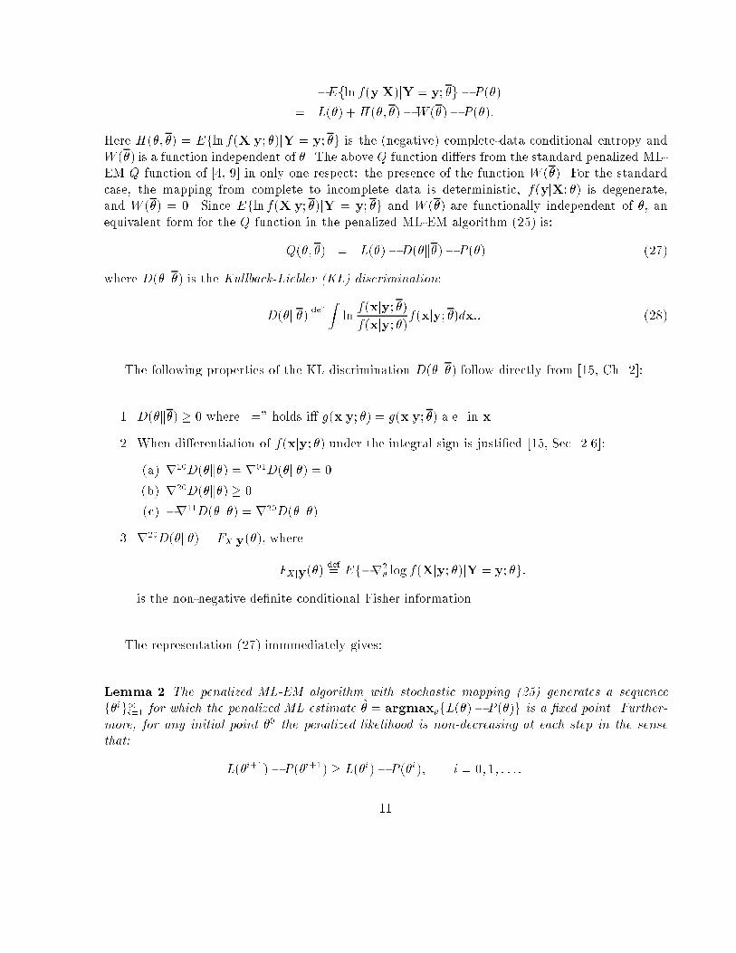
�Efln f(yjX)jY = y; �g � P (�)
= L(�) +H(�; �)�W (�)� P (�):
Here H(�; �) = Efln f(Xjy; �)jY = y; �g is the (negative) complete-data conditional entropy and
W (�) is a function independent of �. The above Q function di�ers from the standard penalized ML-
EM Q function of [4, 9] in only one respect: the presence of the function W (�). For the standard
case, the mapping from complete to incomplete data is deterministic, f(yjX; �) is degenerate,
and W (�) = 0. Since Efln f(Xjy; �)jY = y; �g and W (�) are functionally independent of �, an
equivalent form for the Q function in the penalized ML-EM algorithm (25) is:
Q(�; �) = L(�)�D(�k�)� P (�) (27)
where D(�k�) is the Kullback-Liebler (KL) discrimination:
D(�k�)
def
=
Z
ln
f(xjy; �)
f(xjy; �)
f(xjy; �)dx:: (28)
The following properties of the KL discrimination D(�k�) follow directly from [15, Ch. 2]:
1. D(�k�) � 0 where \=" holds i� g(xjy; �) = g(xjy; �) a.e. in x.
2. When di�erentiation of f(xjy; �) under the integral sign is justi�ed [15, Sec. 2.6]:
(a) r
10
D(�k�) = r
01
D(�k�) = 0
(b) r
20
D(�k�) � 0
(c) �r
11
D(�k�) = r
20
D(�k�)
3. r
20
D(�k�) = F
Xjy
(�), where
F
Xjy
(�)
def
= Ef�r
2
�
log f(Xjy; �)jY = y; �g:
is the non-negative de�nite conditional Fisher information.
The representation (27) immmediately gives:
Lemma 2 The penalized ML-EM algorithm with stochastic mapping (25) generates a sequence
f�
i
g
1
i=1
for which the penalized ML estimate
^
� = argmax
�
fL(�)� P (�)g is a �xed point. Further-
more, for any initial point �
0
the penalized likelihood is non-decreasing at each step in the sense
that:
L(�
i+1
)� P (�
i+1
) � L(�
i
)� P (�
i
); i = 0; 1; : : : :
11

Proof of Lemma 2:
Fix i and let �
i
=
^
�. Then:
�
i+1
= argmax
�
fL(�)�D(�k
^
�)� P (�)g
Since L(�) � P (�) and �D(�k
^
�) individually take their maximum values at the same point � =
^
�
we have �
i+1
= �
i
=
^
�. By induction we thus obtain �
n
=
^
� for all n > i. The monotonic increase
in penalized likelihood follows from the chain of inequalities:
0 � Q(�
i+1
; �
i
)� Q(�
i
; �
i
)
= (L(�
i+1
)� P (�
i+1
))� (L(�
i
)� P (�
i
))
�D(�
i+1
; �
i
) +D(�
i
; �
i
)
� (L(�
i+1
)� P (�
i+1
))� (L(�
i
)� P (�
i
))
where the last inequality is a consequence of the inequality: D(�; �
i
) � D(�
i
; �
i
) = 0 for all �. 2
We will need the following de�nitions:
De�nition 2 For
^
� = argmax
�
fL(�) � P (�)g the penalized ML estimate de�ne the symmetric
Hessian matrices:
Q
def
= �r
20
Q(
^
�;
^
�)
L
def
= �r
2
^
�
L(
^
�)
P
def
= r
2
^
�
P (
^
�)
D
def
= r
20
D(
^
�k
^
�): (29)
The following relations follow directly from (27) and properties of the KL discrimination:
Q = L +P+D
r
11
Q(
^
�;
^
�) = �D: (30)
Theorem 2 Assume: i) the penalized ML estimate
^
� = argmax
�
fL(�) � P (�)g occurs in the
interior of the set �; ii) for all � 2 �, the maximum max
�
Q(�; �) is achieved on the interior of
the set �; iii) L(�), P (�), and D(�k�) are twice continuously di�erentiable in � 2 � and � 2 �
and L + P = �r
2
^
�
[L(
^
�) � P (
^
�)] > 0. Let the point �
0
initialize the EM algorithm with stochastic
mapping (25).
12

1. If the positivity condition (8) is satis�ed then the sucessive di�erences ��
i
= �
i
�
^
� of the A
algorithm obey the recursion (10).
2. If �
0
2 R
+
then k��
i
k converges monotonically to zero with at least linear rate and
3. ��
i
asymptotically converges to zero with root convergence factor
�
�
I�Q
�1
[L+P]
�
=
�
�
�
�
�
�
�
�
�
�
�
�
I�Q
�
1
2
[L +P]Q
�
1
2
�
�
�
�
�
�
�
�
�
�
�
�
2
which is strictly less than one.
Proof of Theorem 2
By Lemma 2, in the notation of Theorem 1, the EM algorithm has a �xed point at �
�
=
^
�.
Furthermore, since Q(�; �) = L(�) �D(�k�) � P (�), assumption iii of Theorem 2 guarantees that
Q(�; �) is twice continuously di�erentiable in both arguments. Thus the assumptions of Theorem 1
are satis�ed and item 1 of Theorem 2 follows. Now by Theorem 1 the root convergence factor is given
by �
�
�[r
20
Q(
^
�;
^
�)]
�1
r
11
Q(
^
�;
^
�)
�
. >From identities (29) and (30) �[r
20
Q(
^
�;
^
�)]
�1
r
11
Q(
^
�;
^
�) =
Q
�1
D = [D+L+P]
�1
D = I�Q
�1
[L+P]. Since L+P is positive de�nite and D is non-negative
de�nite (property 2.b of the KL discrimination), Lemma 3 (Appendix) asserts that the eigenvalues
of Q
�1
D are in the range [0; 1). Furthermore, I�Q
�1
[L + P] is similar to the symmetric matrix
I�Q
�
1
2
[L+P]Q
�
1
2
and therefore these two matrices have identical eigenvalues. Since �(A) = jjjAjjj
2
for any real symmetric non-negative matrix A the theorem follows. 2
Note that when the penalty function induces coupling between parameters, the M-step of the EM
"algorithm" described above can be intractable. The OSL method of Green and the majorization
method of DePierro, both described below, address this di�culty by modifying the Q function.
III.b: Linear Approximation to ML-EM Algorithm
In [2] the unpenalized ML-EM algorithm was formulated for the di�cult case of intensity pa-
rameter estimation for continuous-time �ltered Poisson-Gaussian observations. By selecting the
complete data as the unobservable Poisson increment process fdN
t
g
t2[0;T ]
over the time interval
[0; T ], an ML-EM algorithm was derived of the form:
�
i+1
= argmax
�
Q(�; �
i
); i = 1; 2; : : : (31)
where
Q(�; �)
def
=
Z
T
0
^
�(tjy; �) ln�(tj�)dt (32)
13

and �(tj�) is the Poisson point process intensity over time t 2 [0; T ] and parameterized by �,
and
^
�(tjy; �) = EfdN
t
jY = y; �g is the conditional expectation of the Poisson increment process
given Y = y and � = �, i.e. the minimum mean-square error estimate of N
t
. Unfortunately the
computation of the conditional mean estimator proved to be intractible and instead the best linear
estimator
~
�(t; �jy; �) was substituted into (32):
~
Q(�; �)
def
=
Z
T
0
~
�(tjy; �) ln�(tj�)dt
While the algorithm resulting from replacing Q by
~
Q is no longer an ML-EM algorithm, and
the ML estimate may not even be a �xed point, it belongs to the class of A algorithms (1) for
which Theorem 1 can be applied to establish monotone convergence properties and asymptotic
convergence rate. In particular, with �
�
a �xed point, the asymptotic convergence rate to �
�
is
�
�
[r
20
~
Q(�
�
; �
�
)]
�1
r
11
~
Q(�
�
; �
�
)
�
.
III.c: One-Step-Late (OSL) Penalized ML-EM
Green [9, 10] proposed an approximation, which he called the one-step-late (OSL) algorithm,
for the case of tomographic image reconstruction with Poisson data and a Gibbs prior for which
the M step of the penalized ML-EM algorithm is intractible. Green's algorithm is equivalent to
linearizing the prior ln f(�) about the previous iterate �
i
in (25):
�
i+1
=
8
>
<
>
:
argmax
�
fEfln f(X; �)jY; �
i
g+r
�
i
ln f(�
i
)(� � �
i
)g ; i = 1; 2; : : :
or
argzero
�
fr
�
Efln f(X; �)jY; �
i
g+r
�
i
f(�
i
)g ; i = 1; 2; : : :
: (33)
Again Theorem 1 is applicable by identifying Q in the theorem with the function Efln f(X; �)jY; �
i
g+
r
�
iln f(�
i
)(�� �
i
) in (33). If the OSL algorithm converges to a �xed point �
�
the asymptotic con-
vergence rate is:
�
�
[r
20
Q(�
�
; �
�
)]
�1
[r
11
Q(�
�
; �
�
) +r
2
�
i
ln f(�
�
)]
�
= �
�
[L+D]
�1
[D�P]
�
which is identical to the result cited in [10] for the standard case of deterministic complete/incomplete
data mapping and the Gibbs prior f(�) = expf��V (�)g.
IV. APPLICATIONS
We consider two separate applications: the linear Gaussian model and the PET image re-
construction model. These two cases involve complete and incomplete data sets with Gaus-
sian/Gaussian and Poisson/Poisson statistics, respectively.
14
IV.a. Linear Gaussian Model
Consider the following linear Gaussian model:
Y = G� +W
y
(34)
where � 2 � = IR
p
is a p-element parameter vector, G is an m � p matrix with full column rank
p � m, and W
y
is an m-dimensional zero mean Gaussian noise with positive de�nite covariance
�
yy
. The unpenalized ML estimator of � given Y is the weighted least squares estimator:
^
� = [G
T
�
�1
yy
G]
�1
G
T
�
�1
yy
Y: (35)
Next consider decomposing the matrix G into the matrix product BC where the m�n matrix
B has full row rank m, the n � p matrix C has full column rank p, and p � m � n. With this
decomposition we can de�ne a complete-incomplete data model associated with (34):
Y = BX+W (36)
X = C� +W
x
(37)
where the m-element vector W and the n-element vector W
x
are jointly Gaussian with zero mean
and �-independent positive de�nite covariance matrix E
�
("
W
W
x
#
[WW
x
]
)
. These assumptions
guarantee that � be identi�able in the noiseless regime when W
x
andW are vectors of zeroes. The
model (36) is of interest to us since the non-zero noiseW case is not covered by the standard ML-EM
algorithm assumptions. On the other hand, the Gaussian complete/incomplete data mapping (36)
speci�es Y as the output of a simple additive noise channel with input X; a complete-incomplete
data model for which our theory directly applies.
For the Gaussian model (36) the conditional distribution of Y given X = x is speci�ed by a
m-variate Gaussian density N (�;�) with vector location parameter:
� = Bx+E[WjX = x; �]
= Bx+�
yx
�
�1
xx
[x�C�]
and matrix scale parameter:
� = �
yy
� �
T
xy
�
�1
xx
�
xy
:
By assumption the scale parameter � is functionally independent of �. However, unless �
nx
= 0
the location parameter � generally depends on �. To ensure that the conditional density of Y given
X = x be independent of � it is required that W and W
x
be uncorrelated. Under this condition
(36) is a valid complete-incomplete data model.
15

The complete data log-likelihood is:
ln f(x; �) = �
1
2
(x�C�)
T
�
�1
xx
(x�C�) �
1
2
ln j�
xx
j:
Now the unpenalized ML-EM algorithm is of the form (25) with:
Q(�; �) = E[ln f(X; �)jY; �] (38)
= �
1
2
(E[XjY; �]�C�)
T
�
�1
xx
(E[XjY; �]�C�)
�
1
2
E
h
(X�E[XjY; �])
T
�
�1
xx
(X�E[XjY; �])
�
�
�Y; �
i
�
1
2
ln j�
xx
j
= �
1
2
(E[XjY; �]�C�)
T
�
�1
xx
(E[XjY; �]�C�) +K(Y; �)
where K(Y; �) is functionally independent of �. The conditional expectation in (38) has the form:
E[XjY; �
i
] = [I� �
xy
�
�1
yy
B]C � �
i
+ �
xy
�
�1
yy
Y (39)
= [I� �
xx
B
T
�
�1
yy
B]C � �
i
+�
xx
B
T
�
�1
yy
Y: (40)
It is easily veri�ed that:
�r
20
Q(�; �) = C
T
�
�1
xx
C
= F
X
and
r
11
Q(�; �) = C
T
�
�1
xx
C�C
T
B
T
�
�1
yy
BC (41)
= C
T
�
�1
xx
C�C
T
B
T
[B�
xx
B
T
+ �
nn
]
�1
BC (42)
= F
X
� F
Xjy
(43)
where F
X
= Ef�r
2
�
ln f(X; �)g and F
Xjy
= Ef�r
2
�
ln f(XjY; �)jY = y; �g are unconditional and
conditional Fisher information matrices associated with X.
Since the matrices r
11
Q and r
20
Q are functionally independent of � and � the matrices A
1
=
A
1
= M
1
and A
2
= A
2
= M
2
de�ned in (6) and (7) are given by the �- and �-independent matrices:
M
1
(�; �) = F
X
M
2
(�; �) = F
X
� F
Xjy
:
Now the condition M
1
(�; �) > 0 (8) is satis�ed since C is full rank. Thus we obtain from Theorem
2 the recursion for ��
i
= �
i
�
^
�:
��
i+1
= F
�1
X
[F
X
� F
Xjy
] ���
i
This is equivalent to:
F
1
2
X
��
i+1
= F
�
1
2
X
[F
X
� F
Xjy
]F
�
1
2
X
� F
1
2
X
��
i
: (44)
16

Take the Euclidean norm of both sides of (44) to obtain:
k��
i+1
k �
�
�
�
�
�
�
�
�
�
�
�
�
F
�
1
2
X
[F
X
� F
Xjy
]F
�
1
2
X
�
�
�
�
�
�
�
�
�
�
�
�
2
� k��
i
k (45)
where jjj�jjj
2
is the matrix-2 norm and k�k is the weighted Euclidean norm de�ned on vectors u 2 IR
p
:
kuk
def
= u
T
F
X
u: (46)
Applying the Sherman-Morrisey-Woodbury [7] identity to the matrix F
X
� F
Xjy
(43) we see
that it is symmetric positive de�nite:
�F
def
= F
X
� F
Xjy
= C
T
[�
�1
xx
�B
T
[B�
xx
B+�
nn
]
�1
B]C = C
T
�
�1
xx
[�
�1
xx
+B
T
�
�1
nn
B]
�1
�
�1
xx
C
> 0: (47)
Thus F
�
1
2
X
[F
X
� F
Xjy
]F
�
1
2
X
is symmetric positive de�nite and therefore:
�
�
�
�
�
�
�
�
�
�
�
�
F
�
1
2
X
[F
X
� F
Xjy
]F
�
1
2
X
�
�
�
�
�
�
�
�
�
�
�
�
2
= �
�
F
�
1
2
X
[F
X
� F
Xjy
]F
�
1
2
X
�
= �
�
I� F
�1
X
F
Xjy
�
= �
�
I� [�F+ F
Xjy
]
�1
F
Xjy
�
< 1
where we have used Lemma 3 and the fact that �F > 0 and F
Xjy
� 0. Therefore from (45):
k��
i+1
k < k��
i
k
and the ML-EM algorithm converges monotonically in the norm k � k (46) for all initial points
�
0
. Therefore it converges globally in any norm. The asymptotic convergence rate is seen to be
�
�
I� F
�1
X
F
Xjy
�
. We have thus established the following:
Theorem 3 The ML-EM algorithm for the Gaussian complete/incomplete data mapping de�ned
by (36) globally converges everywhere in � = IR
p
to the ML estimate. Furthermore convergence is
monotone in the norm kuk
def
= u
T
F
X
u and the root convergence factor is �(A) < 1 where A is the
matrix:
A = I� F
�1
X
F
Xjy
(48)
where
F
X
def
= C
T
�
�1
xx
C (49)
F
Xjy
def
= C
T
B
T
[B�
xx
B+�
nn
]
�1
BC: (50)
17
Finally, it is useful to remark that due to the form of A (48), the spectral radius �(A) can
only increase as the covariance �
nn
of the channel noise W increases. We therefore conclude that
while increased channel noise does not a�ect the region of monotone convergence of the ML-EM
algorithm it does adversely a�ect the rate of convergence for the Gaussian model (36).
IV.b. PET Image Reconstruction
In the PET problem the objective is to estimate the intensity � = [�
1
; : : : ; �
p
]
T
, �
b
� 0, governing
the number of gamma-ray emissions N = [N
1
; : : : ;N
p
]
T
over an imaging volume of p pixels. The
estimate of � must be based on the projection data Y = [Y
1
; : : : ;Y
m
]
T
. BothN and Y are Poisson
distributed:
P (N; �) =
p
Y
b=1
[�
b
]
N
b
!
N
b
e
��
b
;
P (Y; �) =
m
Y
d=1
[�
d
]
Y
d
!
Y
d
e
��
d
(51)
where �
d
= E
�
[Y
d
] is the Poisson intensity for detector d:
�
d
=
p
X
b=1
P
djb
�
b
and P
djb
is the transition probability corresponding to emitter location b and detector location d.
To ensure a unique ML estimate we assume that m � p, the m � p system matrix [[P
djb
]] is full
rank, and (�
d
, Y
d
) are strictly positive for all d = 1; : : : ; m.
The standard choice of complete data X for estimation of � via the EM algorithm is the set
fN
db
g
m;p
d=1;b=1
, where N
db
denotes the number of emissions in pixel b which are detected at detector
d [23, 17]. This complete data is related to the incomplete data via the deterministic many-to-
one mapping: N
d
=
P
p
b=1
N
db
, d = 1; : : : ; m. It is easily established that fN
db
g are independent
Poisson random variables with intensity E
�
fN
db
g = P
djb
�
b
, d = 1; : : : ; m, b = 1; : : : ; p and that the
conditional expectation Efln f(X; �)jy; �
i
g of the complete data log-likelihood given the incomplete
data is [10]:
Efln f(X; �)jY; �
i
g =
m
X
d=1
p
X
b=1
"
Y
d
P
djb
�
i
b
�
i
d
ln(P
djb
�
b
)� P
djb
�
b
#
where �
i
d
=
P
p
b=1
�
i
b
P
bjd
. For a penalty function P (�) the Q function for the penalized ML-EM
algorithm is:
Q(�; �
i
) = Efln f(X; �)jY; �
i
g � P (�);
18

which yields a sequence of estimates �
i
, i = 1; 2; : : : of �. In order to obtain asymptotic convergence
properties using Theorem 2 it will be necessary to assume �
i
lies on the interior of �, i.e. �
i
lies
in the strictly positive orthant, for all i > 0 . This assumption only holds when the unpenalized or
penalized ML estimate
^
� lies in the interior of �, a condition which is usually not met throughout
the image. For example, when
P
m
d=1
P
bjd
= 0 the pixel b is outside the �eld of view and it is easily
established that
^
�
b
= 0. Therefore, for the following analysis to hold, the pixels for which
^
� lies on
the boundary must be eliminated from the vector �
i
.
Under these assumptions
�r
20
Q(�; �
i
) = diag
b
�
�
i
b
�
b
�
� [B(�
i
) +C(�
i
)] � diag
b
�
�
i
b
�
b
�
+ P(�) (52)
r
11
Q(�; �
i
) = diag
b
�
�
i
b
�
b
�
�C(�
i
) (53)
where, similar to the de�nition in [10], B(�
i
) is the positive de�nite p� p matrix:
B(�
i
)
def
=
m
X
d=1
Y
d
[�
i
d
]
2
P
dj�
P
T
dj�
;
B(�
i
) +C(�
i
) is the p� p positive de�nite matrix
B(�
i
) +C(�
i
)
def
= diag
b
1
�
i
b
m
X
d=1
Y
d
P
djb
�
i
d
!
:
and
P(�)
def
= r
2
�
P (�):
The matrices A
1
(�; �
i
) and A
2
(�; �
i
) de�ned in (7) are obtained by taking the k-th row of
�r
20
Q(�; �
i
) and the k-th row of r
11
Q(�; �
i
) and replacing � and �
i
with �(t) = t
k
� + (1 � t
k
)
^
�
and �
i
(t) = t
k
�
i
+ (1� t
k
)
^
�, respectively, k = 1; : : : ; p. This gives:
A
1
(�; �
i
) = diag
b
�
�
i
b
(t
b
)
�
b
(t
b
)
�
� [B
t
+C
t
] � diag
b
�
�
i
b
(t
b
)
�
b
(t
b
)
�
+P
t
(54)
A
2
(�; �
i
) = diag
b
�
�
i
b
(t
b
)
�
b
(t
b
)
�
�C
t
(55)
where P
t
is the p� p matrix:
P
t
def
= �
2
6
6
4
r
�
@
@�
1
(t
1
)
P (�(t
1
))
.
.
.
r
�
@
@�
p
(t
p
)
P (�(t
p
))
3
7
7
5
; (56)
19

B
t
is the non-negative de�nite p� p matrix:
B
t
def
=
m
X
d=1
Y
d
diag
b
�
1
�
i
d
(t
b
)
�
P
dj�
P
T
dj�
diag
b
�
1
�
i
d
(t
b
)
�
; (57)
B
t
+C
t
is the positive de�nite p� p matrix:
B
t
+C
t
def
= diag
b
1
�
i
b
(t
b
)
m
X
d=1
Y
d
P
djb
�
i
d
(t
b
)
!
; (58)
and �
i
d
(t
b
)j
def
=
P
p
k=1
�
i
k
(t
b
)P
kjd
.
Now if A
1
(�; �
i
) is invertible for all �, and �
i
we have from (10) of Theorem 1:
��
i+1
= �[A
1
(�
i+1
; �
i
)]
�1
A
2
(�
i+1
; �
i
) ���
i
(59)
= diag
b
�
i+1
b
(t
b
)
�
i
b
(t
b
)
!
� [B
t
+C
t
+ diag
b
�
i+1
b
(t
b
)
�
i
b
(t
b
)
!
P
t
diag
b
�
i+1
b
(t
b
)
�
i
b
(t
b
)
!
]
�1
C
t
���
i
where t = [t
1
; : : : ; t
p
]
T
is a function of �
i
; �
i+1
;
^
�. Unfortunately, it can be shown that for any �
i
,
sup
�2�
jjjA
1
(�; �
i
)]
�1
A
2
(�; �
i
)jjj is unbounded for any Euclidean-type norm of the form kuk
2
= u
T
Du
where D is positive de�nite. Thus the monotone convergence part of Theorem 2 fails to apply. This
suggests that to establish monotone convergence properties of the PET EM algorithm, we should
consider other parameterizations of �.
Consider the alternative parameterization de�ned by the logarithmic transformation g::
� = ln � = [ln �
1
; : : : ; ln �
p
]
T
:
The inverse of the transformation g(�) = ln � is the exponential transformation
g
�1
(�) = e
�
= [e
�
1
; : : : ; e
�
p
]
T
;
and the Jacobian is the diagonal matrix with diagonal elements:
[J(�)]
bb
= e
��
b
:
Using (54) and (55) we obtain from (22):
��
i+1
= diag
b
�
e
��
i
b
(t
b
)
� h
~
B
t
+
~
C
t
+ diag
b
�
e
�
i+1
b
(t
b
)��
i
b
(t
b
)
�
~
P
t
diag
b
�
e
�
i+1
b
(t
b
)��
i
b
(t
b
)
�i
�1
�
~
C
t
diag
b
�
e
�
i
b
(t
b
)
�
���
i
where
~
B
t
,
~
C
t
and
~
P
t
are B
t
, C
t
and P
t
of (56)-(58) parameterized in terms of � = �(�) and
�(t
b
) = t
b
� + (1 � t
b
)�̂ , b = 1; : : : ; p. Using the facts that �
b
= ln �
b
and �(t
b
) = ln �(t
b
) for some
t
b
2 [0; 1], b = 1; : : : ; p, we can express the above in terms of the original parameterization to obtain:
(60)
� ln �
i+1
= D
t
�1
[B
t
+C
t
+R
T
t
P
t
R
t
]
�1
C
t
D
t
�� ln �
i
;
20

where
D
t
def
= diag
b
�
�
i
b
(t
b
)
�
R
t
def
= diag
b
�
i+1
b
(t
b
)
�
i
b
(t
b
)
!
and � ln � is the vector:
� ln �
def
= ln � � ln
^
�:
In (60) we have dropped the overline in t for notational simplicity. We divide subsequent treatment
into the unpenalized and penalized cases:
Unpenalized ML-EM
For the unpenalized case P
t
= 0, so that B
t
+C
t
+P
t
= B
t
+C
t
is symmetric positive de�nite
and we have from (60):
[B
t
+C
t
]
1
2
D
t
�� ln �
i+1
(61)
= [B
t
+C
t
]
�
1
2
C
t
[B
t
+C
t
]
�
1
2
� [B
t
+C
t
]
1
2
D
t
�� ln �
i
Taking the Euclidean norm of both sides of (61) we obtain:
�
� ln �
i+1
�
T
D
T
t
[B
t
+C
t
]D
t
�
� ln �
i+1
�
(62)
�
�
�
�
�
�
�
�
�
�
�
�
�
[B
t
+C
t
]
�
1
2
C
t
[B
t
+C
t
]
�
1
2
�
�
�
�
�
�
�
�
�
�
�
�
2
�
�
� ln �
i
�
T
D
T
t
[B
t
+C
t
]D
t
�
� ln �
i
�
= �
�
[B
t
+C
t
]
�1
C
t
�
�
�
� ln �
i
�
T
D
T
t
[B
t
+C
t
]D
t
�
� ln �
i
�
It is easily seen that D
T
t
[B
t
+C
t
]D
t
is the diagonal matrix:
D
T
t
[B
t
+C
t
]D
t
= diag
b
�
i
b
(t
b
)
m
X
d=1
Y
d
P
djb
�
i
d
(t
b
)
!
: (63)
This establishes:
p
X
b=1
�
i
b
(t
b
)
m
X
d=1
Y
d
P
djb
�
i
d
(t
b
)
ln
�
i+1
b
^
�
b
!
2
� �
�
[B
t
+C
t
]
�1
C
t
�
p
X
b=1
�
i
b
(t
b
)
m
X
d=1
Y
d
P
djb
�
i
d
(t
b
)
ln
�
i
b
^
�
b
!
2
:
21

We next consider the asymptotic form of (62) for small k��
i
k
2
. By using �
i
b
(t
b
) =
^
�
b
+ t
b
��
i
b
and �
i
d
(t
b
) = �̂
d
+O(k��
i
)k
2
) we obtain:
D
T
t
[B
t
+C
t
]D
t
= D
T
[B+C]D+ O(k��
i
k
2
)
= diag
b
^
�
b
m
X
d=1
Y
d
P
djb
�̂
d
!
+ I �O(k��
i
k
2
); (64)
�
�
[B
t
+C
t
]
�1
C
t
�
= �
�
[B+C]
�1
C
�
+O(k��
i
k
2
) (65)
where �̂
d
=
P
p
b=1
P
djb
^
�
b
and D = D
t
j
t=0
, C = C
t
j
t=0
= C(
^
�), B = B
t
j
t=0
= B(
^
�). It is proven in
Appendix B that �
2
1
def
= �([B+C]
�1
C) < 1. Using the asymptotic forms (64) and (64) in (62):
�
� ln �
i+1
�
T
diag
b
^
�
b
m
X
d=1
Y
d
P
djb
�̂
d
!
�
�
� ln �
i+1
� �
1 +O(k��
i
k
2
)
�
(66)
� �
2
1
�
�
� ln �
i
�
T
diag
b
^
�
b
m
X
d=1
Y
d
P
djb
�̂
d
!
�
� ln �
i
�
�
�
1 + O(k��
i
k
2
)
�
:
Identifying the norm k � k de�ned by:
kuk
def
= u
T
diag
^
�
b
m
X
d=1
Y
d
P
djb
�̂
d
!
u
=
p
X
b=1
^
�
b
m
X
d=1
Y
d
P
djb
�̂
d
u
2
b
: (67)
we have the equivalent form:
� ln �
i+1
�
�
1 + O(k��
i
k
2
)
�
: � �
2
1
� ln �
i
�
�
1 +O(k��
i
k
2
)
�
: (68)
Thus if �
i
is su�cently close to
^
�:
� ln �
i+1
<
� ln �
i
(69)
Now it is known that the ML-EM PET algorithm converges [9] so that k�
i
�
^
�k ! 0. As
long as
^
� is strictly positive, the relation (68) asserts that in the �nal iterations of the algorithm
the logarithmic di�erences ln �
i
� ln
^
� converge monotonically to zero relative to the norm (67).
Furthermore the speed of this asymptotic monotone convergence is inversely proportional to �
2
1
=
�([B+C]
�1
C).
The norm k � k in (67) has a simpler equivalent form which is functionally dependent on Y
d
only through
^
�. The PET log-likelihood function ln P (Y; �) (51) has derivative at the maximum
likelihood estimate
^
�:
@
@
^
�
b
lnP (Y;
^
�) =
p
X
d=1
�
Y
d
P
djb
�̂
d
� P
djb
�
; b = 1; : : : ; p: (70)
22

Now since
^
� is a stationary point of lnP (Y; �) this derivative is zero and:
p
X
d=1
Y
d
P
djb
�̂
d
= P
d
where
P
b
def
=
p
X
b=1
P
djb
Thus (69)is equivalent to:
p
X
b=1
P
b
^
�
b
�
ln �
i+1
b
� ln
^
�
b
�
2
<
p
X
b=1
P
b
^
�
b
�
ln �
i
b
� ln
^
�
b
�
2
Finally we note that:
� ln � = ln
�
b
^
�
b
=
�
b
�
^
�
b
^
�
b
+O(j��
b
j)
so that to O(k��
i
k
2
) (68) is equivalent to:
p
X
b=1
P
b
�
i+1
b
�
^
�
b
^
�
b
!
2
<
p
X
b=1
P
b
�
i
b
�
^
�
b
^
�
b
!
2
Assuming the simple case where P
b
=
P
m
d=1
P
djb
= 1 we conclude that asymptotically the vector of
ratios ��
i
=
^
�
def
= [��
i
b
=
^
�
b
; : : : ;��
i
b
=
^
�
b
]
T
converges monotonically to zero in the standard Euclidean
norm.
We summarize these results in the following theorem.
Theorem 4 Assume that the unpenalized PET ML-EM algorithm converges to the strictly positive
limit
^
�. Then, in the �nal iterations the logarithm of sucessive iterates converge monotonically to
log
^
� in the sense that for some su�ciently large positive integer M :
k log �
i+1
� log
^
�k � �
2
1
k log �
i
� log
^
�k; i �M;
where �
2
1
= �([B+C]
�1
C), B = B(
^
�), C = C(
^
�), the norm k � k is de�ned as:
kuk
def
=
p
X
b=1
P
b
^
�
b
u
2
b
:
and P
b
def
=
P
m
d=1
P
djb
.
23

Quadratically Penalized ML-EM
We assume that P (�) =
1
2
�
T
�� where � is a symmetric non-negative de�nite p�pmatrix. There
is no known closed form solution to the M-step of the penalized ML-EM algorithm (23) unless
� is diagonal. Therefore, for non-diagonal � the recursion (23) is only a theoretical algorithm.
Nonetheless, the convergence properties of this theoretical penalized ML-EM algorithm can be
studied using Theorem 2.
Since B
t
+C
t
is positive de�nite, B
t
+C
t
+R
T
t
P
t
R
t
= B
t
+C
t
+ R
t
�R
t
is positive de�nite
and from (60) we have the representation:
[B
t
+C
t
+R
T
t
�R
t
]
1
2
D
t
� ln �
i+1
(71)
= [B
t
+C
t
+R
�T
t
�R
�1
t
]
�
1
2
C
t
� [B
t
+C
t
+R
�T
t
�R
�1
t
]
�
1
2
�[B
t
+C
t
+R
�T
t
�R
�1
t
]
1
2
D
t
� ln �
i
:
Taking the Euclidean norm of both sides
�
� ln �
i+1
�
T
D
T
t
[B
t
+C
t
+R
�T
t
�R
�1
t
]D
t
�
� ln �
i+1
�
(72)
�
�
�
�
�
�
�
�
�
�
�
�
�
[B
t
+C
t
+R
�T
t
�R
�1
t
]
�
1
2
C
t
[B
t
+C
t
+R
�T
t
�R
�1
t
]
�
1
2
�
�
�
�
�
�
�
�
�
�
�
�
2
�
�
� ln �
i
�
T
D
T
t
[B
t
+C
t
+R
�T
t
�R
�1
t
]D
t
�
� ln �
i
�
= �
�
[B
t
+C
t
+R
�T
t
�R
�1
t
]
�1
C
t
�
�
�
� ln �
i
�
T
D
T
t
[B
t
+C
t
+R
�T
t
�R
�1
t
]D
t
�
� ln �
i
�
:
As in our study of unpenalized ML-EM we turn to the asymptotic behavior of the penalized
ML-EM inequality (72). First observe that as before D
T
t
[B
t
+C
t
]D
t
= diag
b
�
^
�
b
P
d=1
Y
d
P
djb
�̂
d
�
+
O(k��
i
k
2
) and:
�
�
[B
t
+C
t
+R
�T
t
�R
�1
t
]
�1
C
t
�
= �
�
[B+C+ �]
�1
C
�
+O(k��
i
k
2
):
Now it is easily shown that since � is non-negative de�nite: �
2
2
def
= � ([B+C+�]
�1
C) � � ([B+C]
�1
C) =
�
2
1
< 1. Therefore, similarly to the unpenalized case we have from (72):
�
� ln �
i+1
�
T
"
diag
b
^
�
b
m
X
d=1
Y
d
P
djb
�̂
d
!
+D
T
�D
#
�
� ln �
i+1
�
�
�
1 +O(k��
i
k
2
)
�
� �
2
2
�
�
� ln �
i
�
T
"
diag
b
^
�
b
m
X
d=1
Y
d
P
djb
�̂
d
!
+D
T
�D
#
�
� ln �
i
�
�
�
1 + O(k��
i
k
2
)
�
;
24

where D
def
= diag
b
(
^
�
b
). Identifying the norm k � k de�ned by:
kuk
def
= u
T
"
diag
^
�
b
m
X
d=1
Y
d
P
djb
�̂
d
!
+ diag
b
(
^
�
b
)�diag
b
(
^
�
b
)
#
u (73)
we have:
� ln �
i+1
�
�
1 +O(k��
i
k
2
)
�
� �
2
1
� ln �
i
�
�
1 + O(k��
i
k
2
)
�
: (74)
>From these results we obtain:
Theorem 5 Assume that the quadratically penalized PET ML-EM algorithm converges to the
strictly positive limit
^
�. Then, in the �nal iterations the logarithm of sucessive iterates converge
monotonically to log
^
� in the sense that for some su�ciently large positive integer M :
k log �
i+1
� log
^
�k � �
2
2
k log �
i
� log
^
�k; i �M;
where �
2
2
def
= � ([B+C+�]
�1
C) � �
2
1
= � ([B+C]
�1
C), B = B(
^
�), C = C(
^
�), and the norm k � k
is de�ned by (73).
V. CONCLUSION
We have presented a methodology for studying the asymptotic convergence properties of EM-
type algorithms. We have indicated how our methods apply to several important EM and ap-
proximate EM algorithms presented in the literature. We have established asymptotic monotone
convergence of the log images and asymptotic rate of convergence for the PET ML-EM and pe-
nalized ML-EM image reconstruction algorithms. A weakness of the theory given here is that it
does not apply to cases where the maximization in the M step is achieved on a boundary of the
parameter space. While there are a certain number of such problems where this theory will not
apply, we believe that the theory will nonetheless be useful for a large number of applications ar-
eas. The theory presented in this paper has recently been applied to evaluating the convergence
properties of a rapidly convergent class of EM-type algorithms called space-alternating generalized
EM (SAGE) algorithms [6].
25
APPENDICES
A. Matrix Lemmas
The following matrix results are used in the paper.
Lemma 3 Let the p�p symmetric matrices A and B be positive de�nite and non-negative de�nite,
respectively, and de�ne the matrix C = A+B. Then the eigenvalues of the matrix C
�1
B all lie in
the interval [0; 1).
Proof: Since the matrix C is positive de�nite there exists a symmetric positive de�nite square
root factor C
1
2
such that C = C
1
2
C
1
2
. Furthermore, since C
�
1
2
BC
�
1
2
is non-negative de�nite:
C
�
1
2
BC
�
1
2
= [I � C
�
1
2
AC
�
1
2
] � 0. Now adding the fact that C
�
1
2
AC
�
1
2
is positive de�nite,
we obtain 0 � C
�
1
2
BC
�
1
2
< I so that all of the eigenvalues of C
�
1
2
BC
�
1
2
are non-negative and
strictly less than one. De�ning S = C
1
2
, observe that C
�1
B = S
�1
�C
�
1
2
BC
�
1
2
� S, so that C
�1
B
and C
�
1
2
BC
�
1
2
are similar matrices. Since similar matrices have identical eigenvalues C
�1
B has
eigenvalues in [0; 1). 2
Lemma 4 Let B be an n � p matrix with full column rank p � n. Then �(A) < 1 implies
�
�
[B
T
B]
�1
B
T
AB
�
< 1.
Proof: We use the following fact: if �(A) < 1 then 0 � AA
T
< I. The following sequence of
inequalities establishes the lemma.
�
2
�
[B
T
B]
�1
B
T
AB
�
= �
2
�
[B
T
B]
�
1
2
B
T
AB[B
T
B]
�
1
2
�
= �
�
[B
T
B]
�
1
2
B
T
A �B[B
T
B]
�1
B
T
�A
T
B[B
T
B]
�
1
2
�
� �
�
[B
T
B]
�
1
2
B
T
AA
T
B[B
T
B]
�
1
2
�
= �
�
[B
T
B]
�1
B
T
AA
T
B
�
= �
�
[B
T
AA
T
B+B
T
[I �AA
T
]B]
�1
B
T
AA
T
B
�
< 1
where the last inequality follows directly from Lemma 3. The inequality on the third line follows
from the fact that the symmtric idempotent matrix B[B
T
B]
�1
B
T
satis�es: 0 � B[B
T
B]
�1
B
T
� I.
2
26

B. PET ML-EM Results
Lemma 5 Let the p-element vectors P
dj�
, d = 1; : : : ; m, span IR
p
and assume m � p. Assume that
�
b
> 0 for all b = 1; : : : ; p and Y
d
> 0 for all d = 1; : : : ; m. De�ne the matrices:
B
def
=
m
X
d=1
Y
d
diag
b
�
1
�
d
�
P
dj�
P
T
dj�
diag
b
�
1
�
d
�
; (75)
and
B+C
def
= diag
b
1
�
b
m
X
d=1
Y
d
P
djb
�
d
!
; (76)
where �
d
=
P
p
k=1
�
k
P
kjd
. Then � ([B+C]
�1
C) � �
2
1
where �
2
1
2 [0; 1).
Proof
Since the P
dj�
's span IR
p
and the Y
d
's are positive the matrix B is positive de�nite. Hence, by
Lemma 3, it will su�ce to show that C is non-negative de�nite. De�ne D = diag
b
(�
b
). Then:
C = diag
b
1
�
b
m
X
d=1
Y
d
P
djb
�
d
!
�
m
X
d=1
Y
d
diag
b
�
1
�
d
�
P
dj�
P
T
dj�
diag
b
�
1
�
d
�
= D
�1
"
m
X
d=1
Y
d
E
d
#
D
�1
where
E
d
def
=
�
diag
b
�
P
djb
�
b
�
d
�
� diag
b
�
�
b
�
d
�
P
dj�
P
T
dj�
diag
b
�
�
b
�
d
��
(77)
Therefore it su�ces to show that E
d
� 0 for all d = 1; : : : ; m. Let u 2 IR
p
be arbitrary. Then
u
T
Eu =
p
X
b=1
u
2
b
P
djb
�
b
�
d
�
p
X
b=1
u
b
P
djb
�
b
�
d
!
2
=
p
X
b=1
P
djb
�
b
�
d
(u
b
� u)
2
� 0
where u
def
=
P
p
b=1
u
b
P
djb
�
b
�
d
and we have used the fact that
P
p
b=1
P
djb
�
b
�
d
= 1. 2
27

References
[1] N. Antoniadis, Timing delay estimation for Poisson-Gaussian processes, PhD thesis, The Uni-
versity of Michigan, Ann Arbor, MI 48109-2122, Oct. 1992.
[2] N. Antoniadis and A. O. Hero, \Time delay estimation for Poisson processes using the EM
algorithm," in Proc. IEEE Int. Conf. Acoust., Speech, and Sig. Proc., San Francisco, 1992.
[3] I. Csiszar and G. Tusnady, \Information geometry and alternating minimization procedures,"
Statistics and Decisions, vol. Supplement Issue No. 1, pp. 205{237, 1984.
[4] A. P. Dempster, N. M. Laird, and D. B. Rubin, \Maximum likelihood from incomplete data
via the EM algorithm," J. Royal Statistical Society, Ser. B, vol. 39, pp. 1{38, 1977.
[5] M. Feder, A. Oppenheim, and E. Weinstein, \Maximum likelihood noise cancelation using the
EM algorithm," IEEE Trans. Acoust., Speech, and Sig. Proc., vol. 37, no. 2, pp. 204{216, Feb.
1989.
[6] J. A. Fessler and A. O. Hero, \Complete data spaces and generalized EM algorithms," in Proc.
IEEE Int. Conf. Acoust., Speech, and Sig. Proc., Minneapolis, MN, April. 1993.
[7] G. H. Golub and C. F. Van Loan, Matrix Computations (2nd Edition), The Johns Hopkins
University Press, Baltimore, 1989.
[8] F. A. Graybill, Matrices with Applications in Statistics, Wadsworth Publishing Co., Belmont
CA, 1983.
[9] P. J. Green, \On the use of the EM algorithm for penalized likelihood estimation," J. Royal
Statistical Society, Ser. B, vol. 52, no. 2, pp. 443{452, 1990.
[10] P. J. Green, \Bayesian reconstructions from emission tomography using a modi�ed EM algo-
rithm," IEEE Trans. on Medical Imaging, vol. 11, no. 1, pp. 81{90, March 1990.
[11] T. Hebert and R. Leahy, \A generalized EM algorithm for 3-D Bayesian reconstruction from
Poisson data using Gibbs priors," IEEE Trans. on Medical Imaging, vol. 8, no. 2, pp. 194{203,
1989.
[12] T. Hebert and R. Leahy, \Statistic-based MAP image reconstruction from Poisson data using
Gibbs priors," IEEE Trans. on Signal Processing, vol. 40, no. 9, pp. 2290{2302, 1992.
[13] R. A. Horn and C. R. Johnson, Matrix Analysis, Cambridge, 1985.
[14] I. A. Ibragimov and R. Z. Has'minskii, Statistical estimation: Asymptotic theory, Springer-
Verlag, New York, 1981.
[15] S. Kullback, Information Theory and Statistics, Dover, 1978.
28

[16] K. Lange, \Convergence of EM image reconstruction algorithms with Gibbs smoothing," IEEE
Trans. on Medical Imaging, vol. 9, no. 4, pp. 439{446, June 1991.
[17] K. Lange and R. Carson, \EM reconstruction algorithms for emission and transmission to-
mography," J. Comp. Assisted Tomography, vol. 8, no. 2, pp. 306{316, April 1984.
[18] M. I. Miller and D. L. Snyder, \The role of likelihood and entropy in incomplete-data prob-
lems: applications to estimating point-process intensities and Toeplitz constrained covari-
ances," IEEE Proceedings, vol. 75, no. 7, pp. 892{907, July 1987.
[19] M. Miller and D. Fuhrmann, \An EM algorithm for directions of arrival estimation for narrow-
band signals in noise," in Proceedings of the SPIE, volume 826, pp. 101{103, 1987.
[20] J. M. Ortega and W. C. Rheinboldt, Iterative Solution of Nonlinear Equations in Several
Variables, Academic Press, New York, 1970.
[21] E. Polak, Computational methods in optimization: a uni�ed approach, Academic Press, Or-
lando, 1971.
[22] M. Segal, E. Weinstein, and B. Musicus, \Estimate-maximize algorithms for multichannel time
delay and signal estimation," IEEE Trans. Acoust., Speech, and Sig. Proc., vol. 39, no. 1, pp.
1{16, Jan. 1991.
[23] L. A. Shepp and Y. Vardi, \Maximum likelihood reconstruction for emission tomography,"
IEEE Trans. on Medical Imaging, vol. MI-1, No. 2, pp. 113{122, Oct. 1982.
[24] C. F. J. Wu, \On the convergence properties of the EM algorithm," Annals of Statistics, vol.
11, pp. 95{103, 1983.
29

List of Figures
Figure 1: A representation for Y as the output of a possibly noisy channel C with input X
30
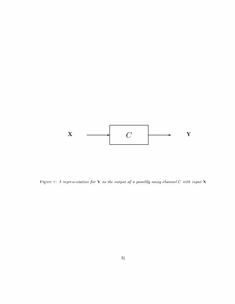
X
-
C
-
Y
Figure 1: A representation for Y as the output of a possibly noisy channel C with input X
31