Embed Size (px)
Citation preview
Asymptotics of some functions arising innumber theory and analysis of algorithms
via computation and Mellin transforms
Richard P. BrentMathematical Sciences Institute, ANU
CARMA, University of Newcastle
incorporating joint work withMichael Coons, Donald Knuth,
Brigitte Vallée and Wadim Zudilin
Presented at Workshop on Mathematics and Computation, Newcastle, 20 June 2015
Richard Brent Asymptotics via computation and Mellin transforms
Abstract
We consider the asymptotic behaviour of some interestingfunctions that arise naturally in
I analysis of algorithms (analysis of the average behaviourof the binary Euclidean algorithm) and in
I number theory (proving algebraic independence resultsusing Mahler’s method).
The asymptotic behaviour of these functions was first exploredvia computation and later explained via Mellin transforms.
Richard Brent Abstract

Summary
The talk has two parts:
I Part I Analysis of the binary Euclidean algorithm(with contributions by Don Knuth and Brigitte Vallée)
I Part II Asymptotics of a Mahler function(with contributions by Michael Coons and Wadim Zudilin)
At first sight the two parts seem unrelated, but by consideringMellin transforms we’ll see that they are very similar.
Richard Brent Summary and Acknowledgements

Part I — Analysis of the binary Euclidean algorithm
The binary Euclidean algorithm is a variant of the classicalEuclidean algorithm for finding greatest common divisors.
It avoids divisions and multiplications, except by powers of two,so is potentially faster than the classical algorithm on a binarymachine.I will describe the binary algorithm and consider its averagecase behaviour. In particular, I will discuss some conjectureswhich were verified computationally in the 1970s and recentlyproved by Ian Morris (2014), extending earlier work by GérardMaze (2005) and by Brigitte Vallée in the 1990s.Analogous results for the classical algorithm were conjecturedby Gauss (1800), and eventually proved by Kuz’min (1928),Lévy (1929) and Wirsing (1974).
Richard Brent Part I — The binary Euclidean algorithm
Part I — Analysis of the binary Euclidean algorithm
The binary Euclidean algorithm is a variant of the classicalEuclidean algorithm for finding greatest common divisors.It avoids divisions and multiplications, except by powers of two,so is potentially faster than the classical algorithm on a binarymachine.
I will describe the binary algorithm and consider its averagecase behaviour. In particular, I will discuss some conjectureswhich were verified computationally in the 1970s and recentlyproved by Ian Morris (2014), extending earlier work by GérardMaze (2005) and by Brigitte Vallée in the 1990s.Analogous results for the classical algorithm were conjecturedby Gauss (1800), and eventually proved by Kuz’min (1928),Lévy (1929) and Wirsing (1974).
Richard Brent Part I — The binary Euclidean algorithm

Part I — Analysis of the binary Euclidean algorithm
The binary Euclidean algorithm is a variant of the classicalEuclidean algorithm for finding greatest common divisors.It avoids divisions and multiplications, except by powers of two,so is potentially faster than the classical algorithm on a binarymachine.I will describe the binary algorithm and consider its averagecase behaviour. In particular, I will discuss some conjectureswhich were verified computationally in the 1970s and recentlyproved by Ian Morris (2014), extending earlier work by GérardMaze (2005) and by Brigitte Vallée in the 1990s.
Analogous results for the classical algorithm were conjecturedby Gauss (1800), and eventually proved by Kuz’min (1928),Lévy (1929) and Wirsing (1974).
Richard Brent Part I — The binary Euclidean algorithm
Part I — Analysis of the binary Euclidean algorithm
The binary Euclidean algorithm is a variant of the classicalEuclidean algorithm for finding greatest common divisors.It avoids divisions and multiplications, except by powers of two,so is potentially faster than the classical algorithm on a binarymachine.I will describe the binary algorithm and consider its averagecase behaviour. In particular, I will discuss some conjectureswhich were verified computationally in the 1970s and recentlyproved by Ian Morris (2014), extending earlier work by GérardMaze (2005) and by Brigitte Vallée in the 1990s.Analogous results for the classical algorithm were conjecturedby Gauss (1800), and eventually proved by Kuz’min (1928),Lévy (1929) and Wirsing (1974).
Richard Brent Part I — The binary Euclidean algorithm
Notation
lg(x) denotes log2(x).
Val2(u) denotes the dyadic valuation of the positive integer u,i.e. the greatest integer j such that 2j | u.
Richard Brent Notation
Notation
lg(x) denotes log2(x).
Val2(u) denotes the dyadic valuation of the positive integer u,i.e. the greatest integer j such that 2j | u.
Richard Brent Notation
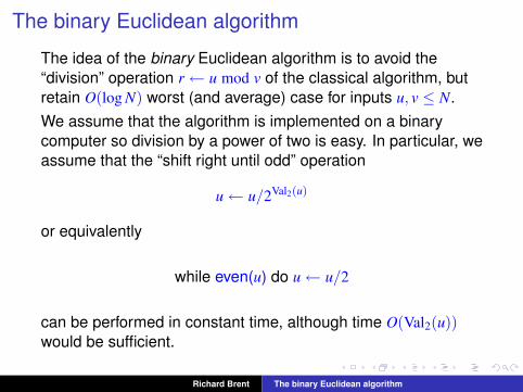
The binary Euclidean algorithm
The idea of the binary Euclidean algorithm is to avoid the“division” operation r ← u mod v of the classical algorithm, butretain O(log N) worst (and average) case for inputs u, v ≤ N.
We assume that the algorithm is implemented on a binarycomputer so division by a power of two is easy. In particular, weassume that the “shift right until odd” operation
u← u/2Val2(u)
or equivalently
while even(u) do u← u/2
can be performed in constant time, although time O(Val2(u))would be sufficient.
Richard Brent The binary Euclidean algorithm
The binary Euclidean algorithm
The idea of the binary Euclidean algorithm is to avoid the“division” operation r ← u mod v of the classical algorithm, butretain O(log N) worst (and average) case for inputs u, v ≤ N.We assume that the algorithm is implemented on a binarycomputer so division by a power of two is easy. In particular, weassume that the “shift right until odd” operation
u← u/2Val2(u)
or equivalently
while even(u) do u← u/2
can be performed in constant time, although time O(Val2(u))would be sufficient.
Richard Brent The binary Euclidean algorithm

Definition of the algorithm
It is easy to take account of the largest power of two dividingthe inputs, so for simplicity we assume that u and v are oddpositive integers.
Following is a simplified version of the algorithm given inKnuth, The Art of Computer Programming, §4.5.2.
Algorithm BB1. t← |u− v|;
if t = 0 return u;B2. t← t/2Val2(t);B3. if u ≥ v then u← t else v← t;
go to B1.
Richard Brent The binary Euclidean algorithm

History
The binary Euclidean algorithm is often attributed to Silver andTerzian (unpublished, 1962) and Stein (1967). However, itseems to go back almost as far as the classical Euclideanalgorithm. Knuth (§4.5.2) quotes a translation of a first-centuryAD Chinese text Chiu Chang Suan Shu on how to reduce afraction to lowest terms:
If halving is possible, take half.
Otherwise write down the denominator and thenumerator, and subtract the smaller from the greater.
Repeat until both numbers are equal.
Simplify with this common value.
This looks very much like Algorithm B !
Richard Brent History
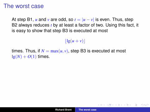
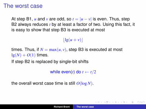
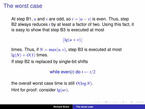
The worst case
At step B1, u and v are odd, so t = |u− v| is even. Thus, stepB2 always reduces t by at least a factor of two. Using this fact, itis easy to show that step B3 is executed at most
blg(u + v)c
times. Thus, if N = max(u, v), step B3 is executed at mostlg(N) + O(1) times.
If step B2 is replaced by single-bit shifts
while even(t) do t← t/2
the overall worst case time is still O(log N).Hint for proof: consider lg(uv).
Richard Brent The worst case
The worst case
At step B1, u and v are odd, so t = |u− v| is even. Thus, stepB2 always reduces t by at least a factor of two. Using this fact, itis easy to show that step B3 is executed at most
blg(u + v)c
times. Thus, if N = max(u, v), step B3 is executed at mostlg(N) + O(1) times.If step B2 is replaced by single-bit shifts
while even(t) do t← t/2
the overall worst case time is still O(log N).
Hint for proof: consider lg(uv).
Richard Brent The worst case
The worst case
At step B1, u and v are odd, so t = |u− v| is even. Thus, stepB2 always reduces t by at least a factor of two. Using this fact, itis easy to show that step B3 is executed at most
blg(u + v)c
times. Thus, if N = max(u, v), step B3 is executed at mostlg(N) + O(1) times.If step B2 is replaced by single-bit shifts
while even(t) do t← t/2
the overall worst case time is still O(log N).Hint for proof: consider lg(uv).
Richard Brent The worst case
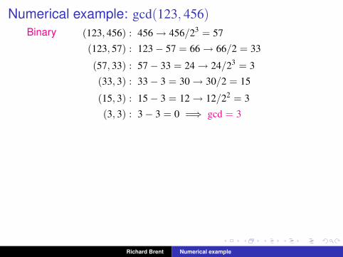
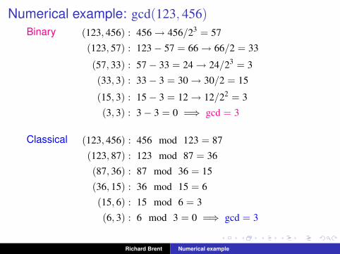
Numerical example: gcd(123, 456)
Binary (123, 456) : 456→ 456/23 = 57
(123, 57) : 123− 57 = 66→ 66/2 = 33
(57, 33) : 57− 33 = 24→ 24/23 = 3
(33, 3) : 33− 3 = 30→ 30/2 = 15
(15, 3) : 15− 3 = 12→ 12/22 = 3
(3, 3) : 3− 3 = 0 =⇒ gcd = 3
Classical (123, 456) : 456 mod 123 = 87
(123, 87) : 123 mod 87 = 36
(87, 36) : 87 mod 36 = 15
(36, 15) : 36 mod 15 = 6
(15, 6) : 15 mod 6 = 3
(6, 3) : 6 mod 3 = 0 =⇒ gcd = 3
Richard Brent Numerical example

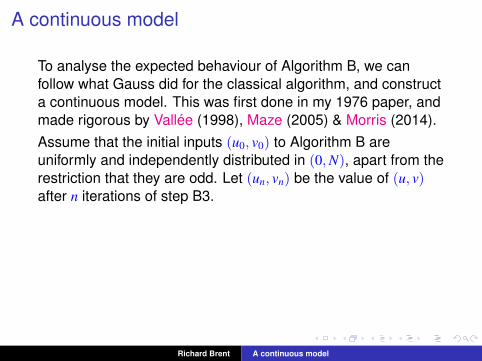
A continuous model
To analyse the expected behaviour of Algorithm B, we canfollow what Gauss did for the classical algorithm, and constructa continuous model. This was first done in my 1976 paper, andmade rigorous by Vallée (1998), Maze (2005) & Morris (2014).
Assume that the initial inputs (u0, v0) to Algorithm B areuniformly and independently distributed in (0,N), apart from therestriction that they are odd. Let (un, vn) be the value of (u, v)after n iterations of step B3.Let
xn =min(un, vn)max(un, vn)
,
and let Fn(x) be the probability distribution function of xn
(in the limit as N →∞). Thus F0(x) = x for x ∈ [0, 1].
Richard Brent A continuous model
A continuous model
To analyse the expected behaviour of Algorithm B, we canfollow what Gauss did for the classical algorithm, and constructa continuous model. This was first done in my 1976 paper, andmade rigorous by Vallée (1998), Maze (2005) & Morris (2014).Assume that the initial inputs (u0, v0) to Algorithm B areuniformly and independently distributed in (0,N), apart from therestriction that they are odd. Let (un, vn) be the value of (u, v)after n iterations of step B3.
Letxn =
min(un, vn)max(un, vn)
,
and let Fn(x) be the probability distribution function of xn
(in the limit as N →∞). Thus F0(x) = x for x ∈ [0, 1].
Richard Brent A continuous model

A continuous model
To analyse the expected behaviour of Algorithm B, we canfollow what Gauss did for the classical algorithm, and constructa continuous model. This was first done in my 1976 paper, andmade rigorous by Vallée (1998), Maze (2005) & Morris (2014).Assume that the initial inputs (u0, v0) to Algorithm B areuniformly and independently distributed in (0,N), apart from therestriction that they are odd. Let (un, vn) be the value of (u, v)after n iterations of step B3.Let
xn =min(un, vn)max(un, vn)
,
and let Fn(x) be the probability distribution function of xn
(in the limit as N →∞). Thus F0(x) = x for x ∈ [0, 1].
Richard Brent A continuous model
Plausible assumption
We make the plausible assumption that Val2(t) takes the value kwith probability 2−k at step B2.
It is a plausible approximation because Val2(t) at step B2depends on the least significant bits of u and v, whereas thecomparison at step B3 depends on the most significant bits, soone would expect the steps to be (almost) independent.A rigorous justification has recently been given by Ian Morris,who shows that the assumption is correct in the limit asN →∞.
Richard Brent A continuous model
Plausible assumption
We make the plausible assumption that Val2(t) takes the value kwith probability 2−k at step B2.It is a plausible approximation because Val2(t) at step B2depends on the least significant bits of u and v, whereas thecomparison at step B3 depends on the most significant bits, soone would expect the steps to be (almost) independent.
A rigorous justification has recently been given by Ian Morris,who shows that the assumption is correct in the limit asN →∞.
Richard Brent A continuous model
Plausible assumption
We make the plausible assumption that Val2(t) takes the value kwith probability 2−k at step B2.It is a plausible approximation because Val2(t) at step B2depends on the least significant bits of u and v, whereas thecomparison at step B3 depends on the most significant bits, soone would expect the steps to be (almost) independent.A rigorous justification has recently been given by Ian Morris,who shows that the assumption is correct in the limit asN →∞.
Richard Brent A continuous model

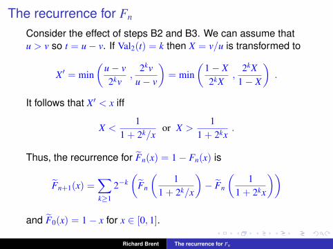
The recurrence for Fn
Consider the effect of steps B2 and B3. We can assume thatu > v so t = u− v. If Val2(t) = k then X = v/u is transformed to
X′ = min(
u− v2kv
,2kv
u− v
)= min
(1− X2kX
,2kX
1− X
).
It follows that X′ < x iff
X <1
1 + 2k/xor X >
11 + 2kx
.
Thus, the recurrence for F̃n(x) = 1− Fn(x) is
F̃n+1(x) =∑k≥1
2−k(
F̃n
(1
1 + 2k/x
)− F̃n
(1
1 + 2kx
))
and F̃0(x) = 1− x for x ∈ [0, 1].
Richard Brent The recurrence for Fn
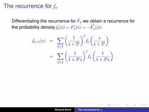
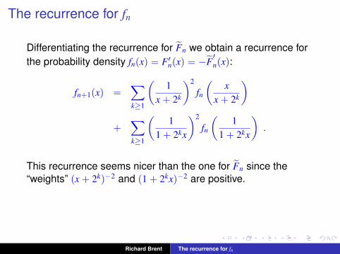
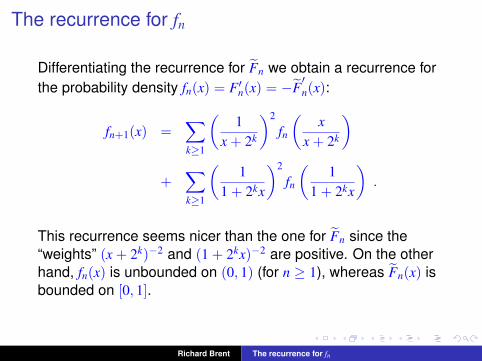
The recurrence for fn
Differentiating the recurrence for F̃n we obtain a recurrence forthe probability density fn(x) = F′n(x) = −F̃
′n(x):
fn+1(x) =∑k≥1
(1
x + 2k
)2
fn
(x
x + 2k
)
+∑k≥1
(1
1 + 2kx
)2
fn
(1
1 + 2kx
).
This recurrence seems nicer than the one for F̃n since the“weights” (x + 2k)−2 and (1 + 2kx)−2 are positive. On the otherhand, fn(x) is unbounded on (0, 1) (for n ≥ 1), whereas F̃n(x) isbounded on [0, 1].
Richard Brent The recurrence for fn
The recurrence for fn
Differentiating the recurrence for F̃n we obtain a recurrence forthe probability density fn(x) = F′n(x) = −F̃
′n(x):
fn+1(x) =∑k≥1
(1
x + 2k
)2
fn
(x
x + 2k
)
+∑k≥1
(1
1 + 2kx
)2
fn
(1
1 + 2kx
).
This recurrence seems nicer than the one for F̃n since the“weights” (x + 2k)−2 and (1 + 2kx)−2 are positive.
On the otherhand, fn(x) is unbounded on (0, 1) (for n ≥ 1), whereas F̃n(x) isbounded on [0, 1].
Richard Brent The recurrence for fn
The recurrence for fn
Differentiating the recurrence for F̃n we obtain a recurrence forthe probability density fn(x) = F′n(x) = −F̃
′n(x):
fn+1(x) =∑k≥1
(1
x + 2k
)2
fn
(x
x + 2k
)
+∑k≥1
(1
1 + 2kx
)2
fn
(1
1 + 2kx
).
This recurrence seems nicer than the one for F̃n since the“weights” (x + 2k)−2 and (1 + 2kx)−2 are positive. On the otherhand, fn(x) is unbounded on (0, 1) (for n ≥ 1), whereas F̃n(x) isbounded on [0, 1].
Richard Brent The recurrence for fn

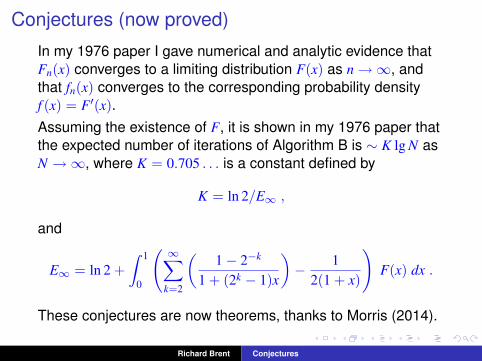
Conjectures (now proved)
In my 1976 paper I gave numerical and analytic evidence thatFn(x) converges to a limiting distribution F(x) as n→∞, andthat fn(x) converges to the corresponding probability densityf (x) = F′(x).
Assuming the existence of F, it is shown in my 1976 paper thatthe expected number of iterations of Algorithm B is ∼ K lg N asN →∞, where K = 0.705 . . . is a constant defined by
K = ln 2/E∞ ,
and
E∞ = ln 2 +∫ 1
0
( ∞∑k=2
(1− 2−k
1 + (2k − 1)x
)− 1
2(1 + x)
)F(x) dx .
These conjectures are now theorems, thanks to Morris (2014).
Richard Brent Conjectures

Conjectures (now proved)
In my 1976 paper I gave numerical and analytic evidence thatFn(x) converges to a limiting distribution F(x) as n→∞, andthat fn(x) converges to the corresponding probability densityf (x) = F′(x).Assuming the existence of F, it is shown in my 1976 paper thatthe expected number of iterations of Algorithm B is ∼ K lg N asN →∞, where K = 0.705 . . . is a constant defined by
K = ln 2/E∞ ,
and
E∞ = ln 2 +∫ 1
0
( ∞∑k=2
(1− 2−k
1 + (2k − 1)x
)− 1
2(1 + x)
)F(x) dx .
These conjectures are now theorems, thanks to Morris (2014).
Richard Brent Conjectures
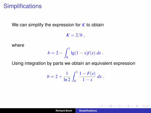
Simplifications
We can simplify the expression for K to obtain
K = 2/b ,
where
b = 2−∫ 1
0lg(1− x)f (x) dx .
Using integration by parts we obtain an equivalent expression
b = 2 +1
ln 2
∫ 1
0
1− F(x)1− x
dx .
Richard Brent Simplifications
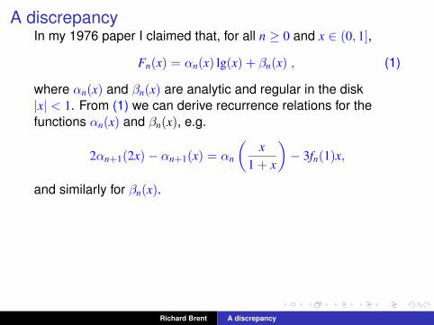
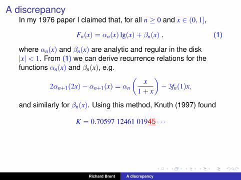
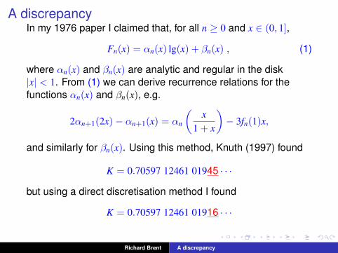
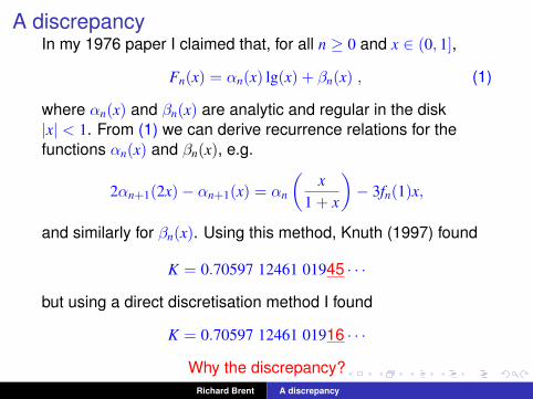
A discrepancyIn my 1976 paper I claimed that, for all n ≥ 0 and x ∈ (0, 1],
Fn(x) = αn(x) lg(x) + βn(x) , (1)
where αn(x) and βn(x) are analytic and regular in the disk|x| < 1. From (1) we can derive recurrence relations for thefunctions αn(x) and βn(x), e.g.
2αn+1(2x)− αn+1(x) = αn
(x
1 + x
)− 3fn(1)x,
and similarly for βn(x).
Using this method, Knuth (1997) found
K = 0.70597 12461 01945 · · ·
but using a direct discretisation method I found
K = 0.70597 12461 01916 · · ·
Why the discrepancy?
Richard Brent A discrepancy
A discrepancyIn my 1976 paper I claimed that, for all n ≥ 0 and x ∈ (0, 1],
Fn(x) = αn(x) lg(x) + βn(x) , (1)
where αn(x) and βn(x) are analytic and regular in the disk|x| < 1. From (1) we can derive recurrence relations for thefunctions αn(x) and βn(x), e.g.
2αn+1(2x)− αn+1(x) = αn
(x
1 + x
)− 3fn(1)x,
and similarly for βn(x). Using this method, Knuth (1997) found
K = 0.70597 12461 01945 · · ·
but using a direct discretisation method I found
K = 0.70597 12461 01916 · · ·
Why the discrepancy?Richard Brent A discrepancy

Some detective work
After a flurry of emails we (Brent and Knuth) tracked down theerror. It was found independently, and at the same time, byFlajolet and Vallée, who were in email contact with us.
(Knuth was in a hurry to finalise the third edition of volume 2of The Art of Computer Programming.)We found that eqn. (1): Fn(x) = αn(x) lg(x) + βn(x) is incorrectfor n ≥ 1. A small oscillatory term, not expressible in this formwith αn(x), βn(x) regular in the disk |x| < 1, is missing!To explain this, we need to consider Mellin transforms.
Richard Brent A discrepancy

Some detective work
After a flurry of emails we (Brent and Knuth) tracked down theerror. It was found independently, and at the same time, byFlajolet and Vallée, who were in email contact with us.(Knuth was in a hurry to finalise the third edition of volume 2of The Art of Computer Programming.)
We found that eqn. (1): Fn(x) = αn(x) lg(x) + βn(x) is incorrectfor n ≥ 1. A small oscillatory term, not expressible in this formwith αn(x), βn(x) regular in the disk |x| < 1, is missing!To explain this, we need to consider Mellin transforms.
Richard Brent A discrepancy
Some detective work
After a flurry of emails we (Brent and Knuth) tracked down theerror. It was found independently, and at the same time, byFlajolet and Vallée, who were in email contact with us.(Knuth was in a hurry to finalise the third edition of volume 2of The Art of Computer Programming.)We found that eqn. (1): Fn(x) = αn(x) lg(x) + βn(x) is incorrectfor n ≥ 1. A small oscillatory term, not expressible in this formwith αn(x), βn(x) regular in the disk |x| < 1, is missing!
To explain this, we need to consider Mellin transforms.
Richard Brent A discrepancy
Some detective work
After a flurry of emails we (Brent and Knuth) tracked down theerror. It was found independently, and at the same time, byFlajolet and Vallée, who were in email contact with us.(Knuth was in a hurry to finalise the third edition of volume 2of The Art of Computer Programming.)We found that eqn. (1): Fn(x) = αn(x) lg(x) + βn(x) is incorrectfor n ≥ 1. A small oscillatory term, not expressible in this formwith αn(x), βn(x) regular in the disk |x| < 1, is missing!To explain this, we need to consider Mellin transforms.
Richard Brent A discrepancy
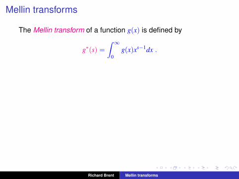
Mellin transforms
The Mellin transform of a function g(x) is defined by
g∗(s) =∫ ∞
0g(x)xs−1dx .
It is easy to see that, if
h(x) =∑k≥1
2−kg(2kx) ,
then the Mellin transform of h is
h∗(s) =∑k≥1
2−k(s+1)g∗(s) =g∗(s)
2s+1 − 1.
Richard Brent Mellin transforms

Mellin transforms
The Mellin transform of a function g(x) is defined by
g∗(s) =∫ ∞
0g(x)xs−1dx .
It is easy to see that, if
h(x) =∑k≥1
2−kg(2kx) ,
then the Mellin transform of h is
h∗(s) =∑k≥1
2−k(s+1)g∗(s) =g∗(s)
2s+1 − 1.
Richard Brent Mellin transforms
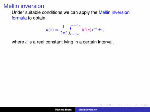
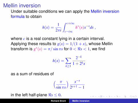
Mellin inversionUnder suitable conditions we can apply the Mellin inversionformula to obtain
h(x) =1
2πi
∫ c+i∞
c−i∞h∗(s)x−sds ,
where c is a real constant lying in a certain interval.
Applying these results to g(x) = 1/(1 + x), whose Mellintransform is g∗(s) = π/ sinπs for 0 < <s < 1, we find
h(x) =∑k≥1
2−k
1 + 2kx
as a sum of residues of( π
sinπs
) x−s
2s+1 − 1
in the left half-plane <s ≤ 0.
Richard Brent Mellin inversion
Mellin inversionUnder suitable conditions we can apply the Mellin inversionformula to obtain
h(x) =1
2πi
∫ c+i∞
c−i∞h∗(s)x−sds ,
where c is a real constant lying in a certain interval.Applying these results to g(x) = 1/(1 + x), whose Mellintransform is g∗(s) = π/ sinπs for 0 < <s < 1, we find
h(x) =∑k≥1
2−k
1 + 2kx
as a sum of residues of( π
sinπs
) x−s
2s+1 − 1
in the left half-plane <s ≤ 0.Richard Brent Mellin inversion
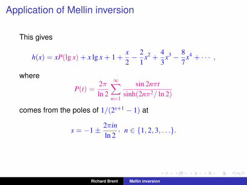
Application of Mellin inversion
This gives
h(x) = xP(lg x) + x lg x + 1 +x2− 2
1x2 +
43
x3 − 87
x4 + · · · ,
where
P(t) =2πln 2
∞∑n=1
sin 2nπtsinh(2nπ2/ ln 2)
comes from the poles of 1/(2s+1 − 1) at
s = −1± 2πinln 2
, n ∈ {1, 2, 3, . . .}.
Richard Brent Mellin inversion

The “wobbles” caused by P(t)
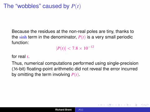
Because the residues at the non-real poles are tiny, thanks tothe sinh term in the denominator, P(t) is a very small periodicfunction:
|P(t)| < 7.8× 10⁻¹²
for real t.
Thus, numerical computations performed using single-precision(36-bit) floating-point arithmetic did not reveal the error incurredby omitting the term involving P(t).
Richard Brent P(t)
The “wobbles” caused by P(t)
Because the residues at the non-real poles are tiny, thanks tothe sinh term in the denominator, P(t) is a very small periodicfunction:
|P(t)| < 7.8× 10⁻¹²
for real t.Thus, numerical computations performed using single-precision(36-bit) floating-point arithmetic did not reveal the error incurredby omitting the term involving P(t).
Richard Brent P(t)
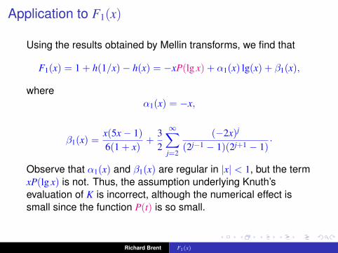
Application to F1(x)
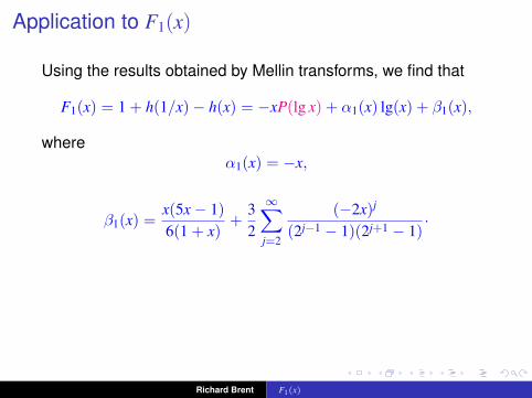
Using the results obtained by Mellin transforms, we find that
F1(x) = 1 + h(1/x)− h(x) = −xP(lg x) + α1(x) lg(x) + β1(x),
whereα1(x) = −x,
β1(x) =x(5x− 1)6(1 + x)
+32
∞∑j=2
(−2x)j
(2j−1 − 1)(2j+1 − 1).
Observe that α1(x) and β1(x) are regular in |x| < 1, but the termxP(lg x) is not. Thus, the assumption underlying Knuth’sevaluation of K is incorrect, although the numerical effect issmall since the function P(t) is so small.
Richard Brent F1(x)
Application to F1(x)
Using the results obtained by Mellin transforms, we find that
F1(x) = 1 + h(1/x)− h(x) = −xP(lg x) + α1(x) lg(x) + β1(x),
whereα1(x) = −x,
β1(x) =x(5x− 1)6(1 + x)
+32
∞∑j=2
(−2x)j
(2j−1 − 1)(2j+1 − 1).
Observe that α1(x) and β1(x) are regular in |x| < 1, but the termxP(lg x) is not. Thus, the assumption underlying Knuth’sevaluation of K is incorrect, although the numerical effect issmall since the function P(t) is so small.
Richard Brent F1(x)
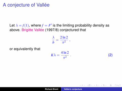
A conjecture of Vallée
Let λ = f (1), where f = F′ is the limiting probability density asabove. Brigitte Vallée (1997/8) conjectured that
λ
b=
2 ln 2π2 ,
or equivalently that
Kλ =4 ln 2π2 . (2)
Richard Brent Vallée’s conjecture

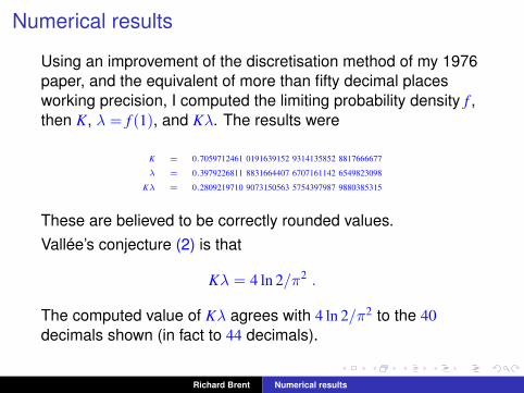
Numerical results
Using an improvement of the discretisation method of my 1976paper, and the equivalent of more than fifty decimal placesworking precision, I computed the limiting probability density f ,then K, λ = f (1), and Kλ. The results were
K = 0.7059712461 0191639152 9314135852 8817666677
λ = 0.3979226811 8831664407 6707161142 6549823098
Kλ = 0.2809219710 9073150563 5754397987 9880385315
These are believed to be correctly rounded values.
Vallée’s conjecture (2) is that
Kλ = 4 ln 2/π2 .
The computed value of Kλ agrees with 4 ln 2/π2 to the 40decimals shown (in fact to 44 decimals).
Richard Brent Numerical results
Numerical results
Using an improvement of the discretisation method of my 1976paper, and the equivalent of more than fifty decimal placesworking precision, I computed the limiting probability density f ,then K, λ = f (1), and Kλ. The results were
K = 0.7059712461 0191639152 9314135852 8817666677
λ = 0.3979226811 8831664407 6707161142 6549823098
Kλ = 0.2809219710 9073150563 5754397987 9880385315
These are believed to be correctly rounded values.Vallée’s conjecture (2) is that
Kλ = 4 ln 2/π2 .
The computed value of Kλ agrees with 4 ln 2/π2 to the 40decimals shown (in fact to 44 decimals).
Richard Brent Numerical results

Proofs
Vallée proved her conjecture under the assumption of aspectral condition.
The conjecture was proved rigorously by Ian Morris (2014)without assuming any spectral condition.The proofs depend on some rather sophisticated functionalanalysis, e.g. the theory of Hardy spaces and Ruelle operators,and are too long to give here – if you are interested, see theoriginal papers by Vallée, Maze and Morris.
Richard Brent Proofs

Proofs
Vallée proved her conjecture under the assumption of aspectral condition.The conjecture was proved rigorously by Ian Morris (2014)without assuming any spectral condition.
The proofs depend on some rather sophisticated functionalanalysis, e.g. the theory of Hardy spaces and Ruelle operators,and are too long to give here – if you are interested, see theoriginal papers by Vallée, Maze and Morris.
Richard Brent Proofs

Proofs
Vallée proved her conjecture under the assumption of aspectral condition.The conjecture was proved rigorously by Ian Morris (2014)without assuming any spectral condition.The proofs depend on some rather sophisticated functionalanalysis, e.g. the theory of Hardy spaces and Ruelle operators,and are too long to give here – if you are interested, see theoriginal papers by Vallée, Maze and Morris.
Richard Brent Proofs
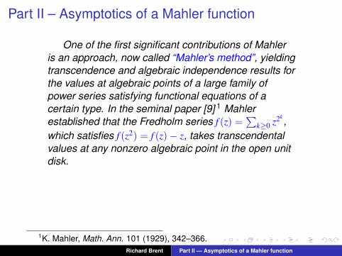
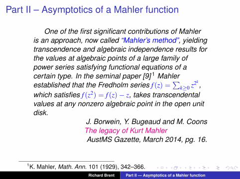
Part II – Asymptotics of a Mahler function
One of the first significant contributions of Mahleris an approach, now called “Mahler’s method”, yieldingtranscendence and algebraic independence results forthe values at algebraic points of a large family ofpower series satisfying functional equations of acertain type. In the seminal paper [9] 1 Mahlerestablished that the Fredholm series f (z) =
∑k≥0 z2k
,which satisfies f (z2) = f (z)− z, takes transcendentalvalues at any nonzero algebraic point in the open unitdisk.
J. Borwein, Y. Bugeaud and M. CoonsThe legacy of Kurt MahlerAustMS Gazette, March 2014, pg. 16.
1K. Mahler, Math. Ann. 101 (1929), 342–366.Richard Brent Part II — Asymptotics of a Mahler function
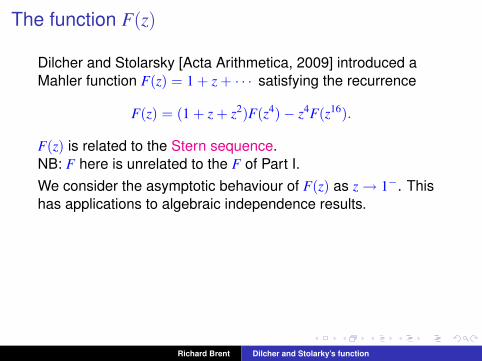
The function F(z)
Dilcher and Stolarsky [Acta Arithmetica, 2009] introduced aMahler function F(z) = 1 + z + · · · satisfying the recurrence
F(z) = (1 + z + z2)F(z4)− z4F(z16).
F(z) is related to the Stern sequence.NB: F here is unrelated to the F of Part I.We consider the asymptotic behaviour of F(z) as z→ 1−. Thishas applications to algebraic independence results.Specifically, BCZ (2015) proved that the functionsF(z),F(z4),F′(z), and F′(z4) are algebraically independentover C(z); it follows (thanks to a result of Kumiko Nishioka) thatF(α),F(α4),F′(α), and F′(α4) are independent over Q for anynonzero algebraic number α in the unit disk.
Richard Brent Dilcher and Stolarky’s function
The function F(z)
Dilcher and Stolarsky [Acta Arithmetica, 2009] introduced aMahler function F(z) = 1 + z + · · · satisfying the recurrence
F(z) = (1 + z + z2)F(z4)− z4F(z16).
F(z) is related to the Stern sequence.
NB: F here is unrelated to the F of Part I.We consider the asymptotic behaviour of F(z) as z→ 1−. Thishas applications to algebraic independence results.Specifically, BCZ (2015) proved that the functionsF(z),F(z4),F′(z), and F′(z4) are algebraically independentover C(z); it follows (thanks to a result of Kumiko Nishioka) thatF(α),F(α4),F′(α), and F′(α4) are independent over Q for anynonzero algebraic number α in the unit disk.
Richard Brent Dilcher and Stolarky’s function

The function F(z)
Dilcher and Stolarsky [Acta Arithmetica, 2009] introduced aMahler function F(z) = 1 + z + · · · satisfying the recurrence
F(z) = (1 + z + z2)F(z4)− z4F(z16).
F(z) is related to the Stern sequence.NB: F here is unrelated to the F of Part I.
We consider the asymptotic behaviour of F(z) as z→ 1−. Thishas applications to algebraic independence results.Specifically, BCZ (2015) proved that the functionsF(z),F(z4),F′(z), and F′(z4) are algebraically independentover C(z); it follows (thanks to a result of Kumiko Nishioka) thatF(α),F(α4),F′(α), and F′(α4) are independent over Q for anynonzero algebraic number α in the unit disk.
Richard Brent Dilcher and Stolarky’s function
The function F(z)
Dilcher and Stolarsky [Acta Arithmetica, 2009] introduced aMahler function F(z) = 1 + z + · · · satisfying the recurrence
F(z) = (1 + z + z2)F(z4)− z4F(z16).
F(z) is related to the Stern sequence.NB: F here is unrelated to the F of Part I.We consider the asymptotic behaviour of F(z) as z→ 1−. Thishas applications to algebraic independence results.
Specifically, BCZ (2015) proved that the functionsF(z),F(z4),F′(z), and F′(z4) are algebraically independentover C(z); it follows (thanks to a result of Kumiko Nishioka) thatF(α),F(α4),F′(α), and F′(α4) are independent over Q for anynonzero algebraic number α in the unit disk.
Richard Brent Dilcher and Stolarky’s function
The function F(z)
Dilcher and Stolarsky [Acta Arithmetica, 2009] introduced aMahler function F(z) = 1 + z + · · · satisfying the recurrence
F(z) = (1 + z + z2)F(z4)− z4F(z16).
F(z) is related to the Stern sequence.NB: F here is unrelated to the F of Part I.We consider the asymptotic behaviour of F(z) as z→ 1−. Thishas applications to algebraic independence results.Specifically, BCZ (2015) proved that the functionsF(z),F(z4),F′(z), and F′(z4) are algebraically independentover C(z);
it follows (thanks to a result of Kumiko Nishioka) thatF(α),F(α4),F′(α), and F′(α4) are independent over Q for anynonzero algebraic number α in the unit disk.
Richard Brent Dilcher and Stolarky’s function
The function F(z)
Dilcher and Stolarsky [Acta Arithmetica, 2009] introduced aMahler function F(z) = 1 + z + · · · satisfying the recurrence
F(z) = (1 + z + z2)F(z4)− z4F(z16).
F(z) is related to the Stern sequence.NB: F here is unrelated to the F of Part I.We consider the asymptotic behaviour of F(z) as z→ 1−. Thishas applications to algebraic independence results.Specifically, BCZ (2015) proved that the functionsF(z),F(z4),F′(z), and F′(z4) are algebraically independentover C(z); it follows (thanks to a result of Kumiko Nishioka) thatF(α),F(α4),F′(α), and F′(α4) are independent over Q for anynonzero algebraic number α in the unit disk.
Richard Brent Dilcher and Stolarky’s function
The Stern sequence
Stern’s diatomic sequence (or Stern-Brocot sequence)is defined by
a0 = 0,
a1 = 1,
a2n = an for n > 0,
a2n+1 = an + an+1 for n > 0.
This sequence has many interesting properties (see the OEISentry A002487). For example, an/an+1 runs through all thereduced nonnegative rationals exactly once.
Richard Brent Digression – the Stern sequence
Some properties of F(z)
Dilcher and Stolarsky (2009) defined F(z) using a polynomialanalogue of the Stern sequence, and deduced the recurrence
F(z) = (1 + z + z2)F(z4)− z4F(z16). (3)
However, for our purposes it is simpler to define F(z) by therecurrence (3) and the auxiliary condition F(z) = 1 + O(z) asz→ 0.Using Mahler’s method, Adamczewski (2010) proved that F(α)is transcendental for every algebraic α, 0 < |α| < 1.Independently, Michael Coons (2010) proved that F(z) is atranscendental function, along with results on transcendenceat algebraic arguments.
Richard Brent Properties of F(z)
Some properties of F(z)
Dilcher and Stolarsky (2009) defined F(z) using a polynomialanalogue of the Stern sequence, and deduced the recurrence
F(z) = (1 + z + z2)F(z4)− z4F(z16). (3)
However, for our purposes it is simpler to define F(z) by therecurrence (3) and the auxiliary condition F(z) = 1 + O(z) asz→ 0.
Using Mahler’s method, Adamczewski (2010) proved that F(α)is transcendental for every algebraic α, 0 < |α| < 1.Independently, Michael Coons (2010) proved that F(z) is atranscendental function, along with results on transcendenceat algebraic arguments.
Richard Brent Properties of F(z)
Some properties of F(z)
Dilcher and Stolarsky (2009) defined F(z) using a polynomialanalogue of the Stern sequence, and deduced the recurrence
F(z) = (1 + z + z2)F(z4)− z4F(z16). (3)
However, for our purposes it is simpler to define F(z) by therecurrence (3) and the auxiliary condition F(z) = 1 + O(z) asz→ 0.Using Mahler’s method, Adamczewski (2010) proved that F(α)is transcendental for every algebraic α, 0 < |α| < 1.
Independently, Michael Coons (2010) proved that F(z) is atranscendental function, along with results on transcendenceat algebraic arguments.
Richard Brent Properties of F(z)

Some properties of F(z)
Dilcher and Stolarsky (2009) defined F(z) using a polynomialanalogue of the Stern sequence, and deduced the recurrence
F(z) = (1 + z + z2)F(z4)− z4F(z16). (3)
However, for our purposes it is simpler to define F(z) by therecurrence (3) and the auxiliary condition F(z) = 1 + O(z) asz→ 0.Using Mahler’s method, Adamczewski (2010) proved that F(α)is transcendental for every algebraic α, 0 < |α| < 1.Independently, Michael Coons (2010) proved that F(z) is atranscendental function, along with results on transcendenceat algebraic arguments.
Richard Brent Properties of F(z)
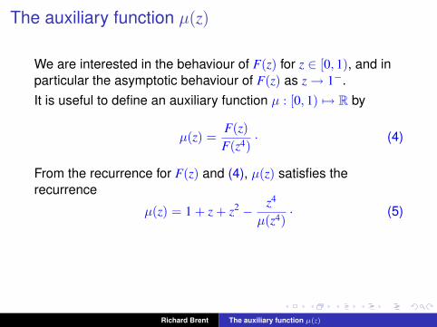
The auxiliary function µ(z)
We are interested in the behaviour of F(z) for z ∈ [0, 1), and inparticular the asymptotic behaviour of F(z) as z→ 1−.
It is useful to define an auxiliary function µ : [0, 1) 7→ R by
µ(z) =F(z)F(z4)
. (4)
From the recurrence for F(z) and (4), µ(z) satisfies therecurrence
µ(z) = 1 + z + z2 − z4
µ(z4). (5)
Our strategy is to analyse the asymptotic behaviour of µ(z) andthen deduce the corresponding behaviour of F(z).
Richard Brent The auxiliary function µ(z)

The auxiliary function µ(z)
We are interested in the behaviour of F(z) for z ∈ [0, 1), and inparticular the asymptotic behaviour of F(z) as z→ 1−.It is useful to define an auxiliary function µ : [0, 1) 7→ R by
µ(z) =F(z)F(z4)
. (4)
From the recurrence for F(z) and (4), µ(z) satisfies therecurrence
µ(z) = 1 + z + z2 − z4
µ(z4). (5)
Our strategy is to analyse the asymptotic behaviour of µ(z) andthen deduce the corresponding behaviour of F(z).
Richard Brent The auxiliary function µ(z)
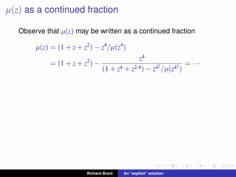
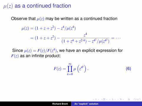
µ(z) as a continued fraction
Observe that µ(z) may be written as a continued fraction
µ(z) = (1 + z + z2)− z4/µ(z4)
= (1 + z + z2)− z4
(1 + z4 + z2·4)− z42/µ(z42)= · · ·
Since µ(z) = F(z)/F(z4), we have an explicit expression forF(z) as an infinite product:
F(z) =∞∏
k=0
µ(
z4k). (6)
In this sense we have an explicit solution for F(z) as an infiniteproduct of continued fractions.
Richard Brent An “explicit” solution
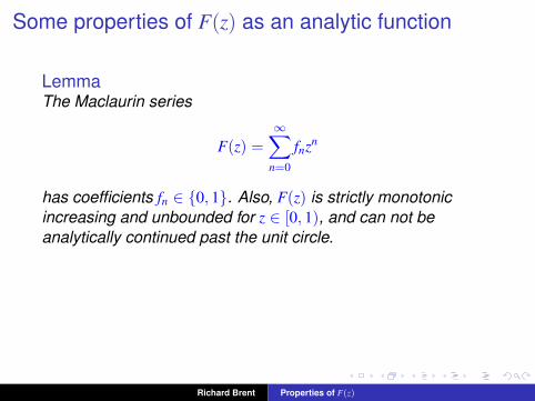
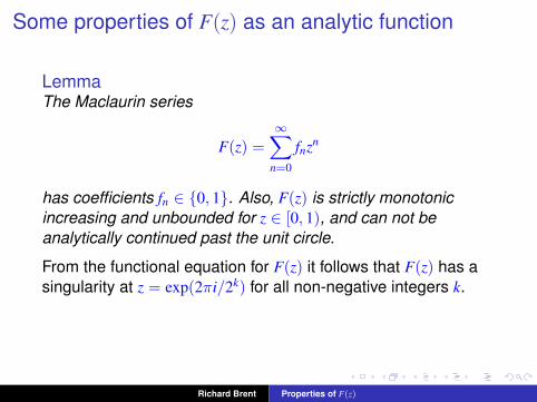
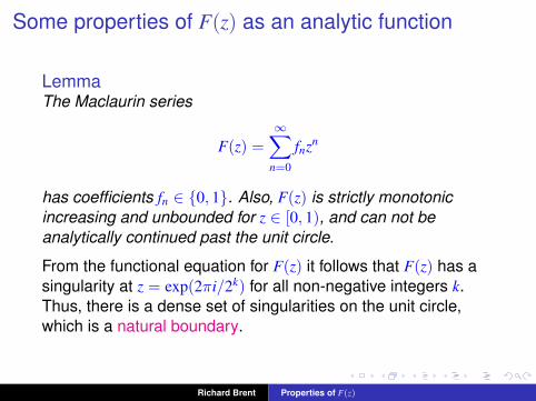
Some properties of F(z) as an analytic function
LemmaThe Maclaurin series
F(z) =∞∑
n=0
fnzn
has coefficients fn ∈ {0, 1}. Also, F(z) is strictly monotonicincreasing and unbounded for z ∈ [0, 1), and can not beanalytically continued past the unit circle.
From the functional equation for F(z) it follows that F(z) has asingularity at z = exp(2πi/2k) for all non-negative integers k.Thus, there is a dense set of singularities on the unit circle,which is a natural boundary.
Richard Brent Properties of F(z)
Some properties of F(z) as an analytic function
LemmaThe Maclaurin series
F(z) =∞∑
n=0
fnzn
has coefficients fn ∈ {0, 1}. Also, F(z) is strictly monotonicincreasing and unbounded for z ∈ [0, 1), and can not beanalytically continued past the unit circle.
From the functional equation for F(z) it follows that F(z) has asingularity at z = exp(2πi/2k) for all non-negative integers k.
Thus, there is a dense set of singularities on the unit circle,which is a natural boundary.
Richard Brent Properties of F(z)
Some properties of F(z) as an analytic function
LemmaThe Maclaurin series
F(z) =∞∑
n=0
fnzn
has coefficients fn ∈ {0, 1}. Also, F(z) is strictly monotonicincreasing and unbounded for z ∈ [0, 1), and can not beanalytically continued past the unit circle.
From the functional equation for F(z) it follows that F(z) has asingularity at z = exp(2πi/2k) for all non-negative integers k.Thus, there is a dense set of singularities on the unit circle,which is a natural boundary.
Richard Brent Properties of F(z)
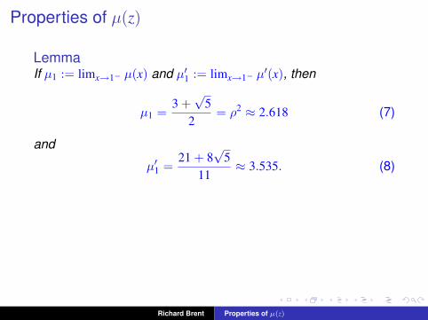
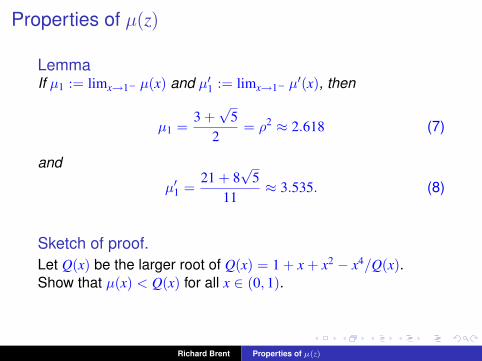
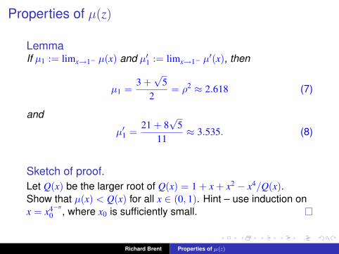
Properties of µ(z)
LemmaIf µ1 := limx→1− µ(x) and µ′1 := limx→1− µ
′(x), then
µ1 =3 +√
52
= ρ2 ≈ 2.618 (7)
and
µ′1 =21 + 8
√5
11≈ 3.535. (8)
Sketch of proof.Let Q(x) be the larger root of Q(x) = 1 + x + x2 − x4/Q(x).Show that µ(x) < Q(x) for all x ∈ (0, 1). Hint – use induction onx = x4−n
0 , where x0 is sufficiently small.
Richard Brent Properties of µ(z)
Properties of µ(z)
LemmaIf µ1 := limx→1− µ(x) and µ′1 := limx→1− µ
′(x), then
µ1 =3 +√
52
= ρ2 ≈ 2.618 (7)
and
µ′1 =21 + 8
√5
11≈ 3.535. (8)
Sketch of proof.Let Q(x) be the larger root of Q(x) = 1 + x + x2 − x4/Q(x).Show that µ(x) < Q(x) for all x ∈ (0, 1).
Hint – use induction onx = x4−n
0 , where x0 is sufficiently small.
Richard Brent Properties of µ(z)
Properties of µ(z)
LemmaIf µ1 := limx→1− µ(x) and µ′1 := limx→1− µ
′(x), then
µ1 =3 +√
52
= ρ2 ≈ 2.618 (7)
and
µ′1 =21 + 8
√5
11≈ 3.535. (8)
Sketch of proof.Let Q(x) be the larger root of Q(x) = 1 + x + x2 − x4/Q(x).Show that µ(x) < Q(x) for all x ∈ (0, 1). Hint – use induction onx = x4−n
0 , where x0 is sufficiently small.
Richard Brent Properties of µ(z)
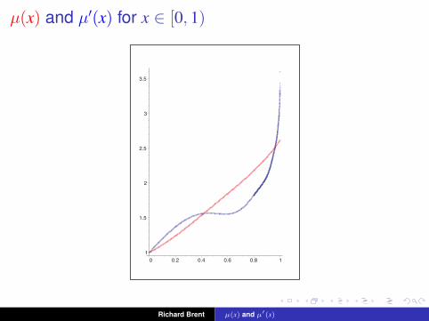
µ(x) and µ′(x) for x ∈ [0, 1)
1
1.5
2
2.5
3
3.5
0 0.2 0.4 0.6 0.8 1
Richard Brent µ(x) and µ′(x)
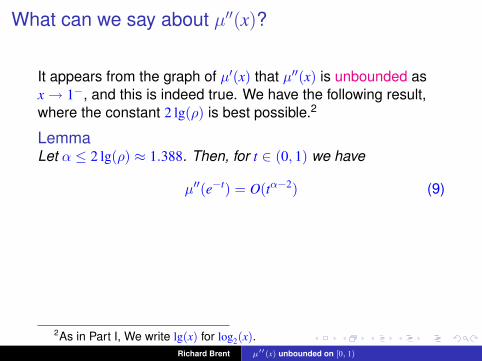
What can we say about µ′′(x)?
It appears from the graph of µ′(x) that µ′′(x) is unbounded asx→ 1−, and this is indeed true. We have the following result,where the constant 2 lg(ρ) is best possible.2
LemmaLet α ≤ 2 lg(ρ) ≈ 1.388. Then, for t ∈ (0, 1) we have
µ′′(e−t) = O(tα−2) (9)
andµ(e−t) = µ1 − tµ′1 + O(tα). (10)
2As in Part I, We write lg(x) for log2(x).Richard Brent µ′′(x) unbounded on [0, 1)
Why the exponent α ≈ 1.388?
Differentiating the recurrence for µ(z) twice, we obtain
µ′′(e−t) = A(t) + B(t)µ′′(e−4t),
where A(t) is bounded, and
B(t) = 16e−10t/µ(e−4t)2 = 16/µ21 + O(t).
The exponent α is chosen so that 16/µ21 ≤ 42−α, since this
inequality is necessary (and sufficient) for the inductive proof togo through.Since µ1 = ρ2, we have to choose α ≤ 2 lg(ρ) ≈ 1.388.
Richard Brent The exponent α
Why the exponent α ≈ 1.388?
Differentiating the recurrence for µ(z) twice, we obtain
µ′′(e−t) = A(t) + B(t)µ′′(e−4t),
where A(t) is bounded, and
B(t) = 16e−10t/µ(e−4t)2 = 16/µ21 + O(t).
The exponent α is chosen so that 16/µ21 ≤ 42−α, since this
inequality is necessary (and sufficient) for the inductive proof togo through.
Since µ1 = ρ2, we have to choose α ≤ 2 lg(ρ) ≈ 1.388.
Richard Brent The exponent α
Why the exponent α ≈ 1.388?
Differentiating the recurrence for µ(z) twice, we obtain
µ′′(e−t) = A(t) + B(t)µ′′(e−4t),
where A(t) is bounded, and
B(t) = 16e−10t/µ(e−4t)2 = 16/µ21 + O(t).
The exponent α is chosen so that 16/µ21 ≤ 42−α, since this
inequality is necessary (and sufficient) for the inductive proof togo through.Since µ1 = ρ2, we have to choose α ≤ 2 lg(ρ) ≈ 1.388.
Richard Brent The exponent α
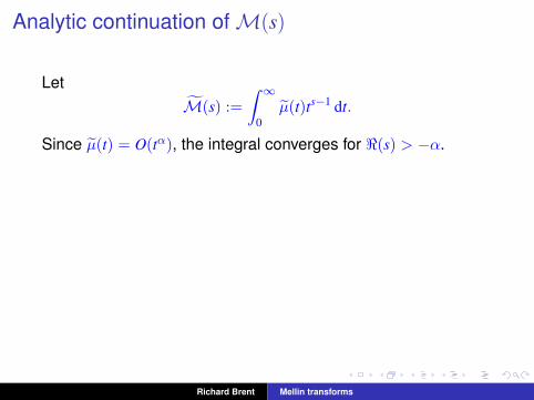
Mellin transforms
Our strategy is to deduce the asymptotic behaviour of µ(z) andF(z) as z→ 1− from certain Mellin transforms.
Specifically, define
F(s) :=∫ ∞
0ln(F(e−t)) ts−1 dt
andM(s) :=
∫ ∞0
ln(µ(e−t)) ts−1 dt.
The integrals converge in the half-plane <(s) > 0. For <(s) ≤ 0we define F(s) andM(s) by analytic continuation (if possible).
Richard Brent Mellin transforms

Mellin transforms
Our strategy is to deduce the asymptotic behaviour of µ(z) andF(z) as z→ 1− from certain Mellin transforms.Specifically, define
F(s) :=∫ ∞
0ln(F(e−t)) ts−1 dt
andM(s) :=
∫ ∞0
ln(µ(e−t)) ts−1 dt.
The integrals converge in the half-plane <(s) > 0. For <(s) ≤ 0we define F(s) andM(s) by analytic continuation (if possible).
Richard Brent Mellin transforms
Mellin transforms
Our strategy is to deduce the asymptotic behaviour of µ(z) andF(z) as z→ 1− from certain Mellin transforms.Specifically, define
F(s) :=∫ ∞
0ln(F(e−t)) ts−1 dt
andM(s) :=
∫ ∞0
ln(µ(e−t)) ts−1 dt.
The integrals converge in the half-plane <(s) > 0.
For <(s) ≤ 0we define F(s) andM(s) by analytic continuation (if possible).
Richard Brent Mellin transforms
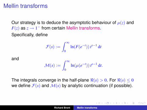
Mellin transforms
Our strategy is to deduce the asymptotic behaviour of µ(z) andF(z) as z→ 1− from certain Mellin transforms.Specifically, define
F(s) :=∫ ∞
0ln(F(e−t)) ts−1 dt
andM(s) :=
∫ ∞0
ln(µ(e−t)) ts−1 dt.
The integrals converge in the half-plane <(s) > 0. For <(s) ≤ 0we define F(s) andM(s) by analytic continuation (if possible).
Richard Brent Mellin transforms
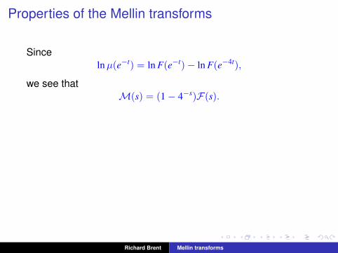
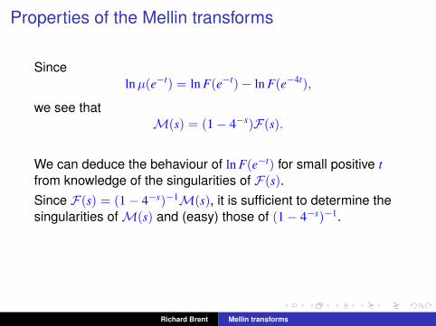
Properties of the Mellin transforms
Sincelnµ(e−t) = ln F(e−t)− ln F(e−4t),
we see thatM(s) = (1− 4−s)F(s).
We can deduce the behaviour of ln F(e−t) for small positive tfrom knowledge of the singularities of F(s).Since F(s) = (1− 4−s)−1M(s), it is sufficient to determine thesingularities ofM(s) and (easy) those of (1− 4−s)−1.First we use the Lemmas above to extend the domain ofdefinition ofM(s) into the left half-plane.
Richard Brent Mellin transforms

Properties of the Mellin transforms
Sincelnµ(e−t) = ln F(e−t)− ln F(e−4t),
we see thatM(s) = (1− 4−s)F(s).
We can deduce the behaviour of ln F(e−t) for small positive tfrom knowledge of the singularities of F(s).
Since F(s) = (1− 4−s)−1M(s), it is sufficient to determine thesingularities ofM(s) and (easy) those of (1− 4−s)−1.First we use the Lemmas above to extend the domain ofdefinition ofM(s) into the left half-plane.
Richard Brent Mellin transforms
Properties of the Mellin transforms
Sincelnµ(e−t) = ln F(e−t)− ln F(e−4t),
we see thatM(s) = (1− 4−s)F(s).
We can deduce the behaviour of ln F(e−t) for small positive tfrom knowledge of the singularities of F(s).Since F(s) = (1− 4−s)−1M(s), it is sufficient to determine thesingularities ofM(s) and (easy) those of (1− 4−s)−1.
First we use the Lemmas above to extend the domain ofdefinition ofM(s) into the left half-plane.
Richard Brent Mellin transforms

Properties of the Mellin transforms
Sincelnµ(e−t) = ln F(e−t)− ln F(e−4t),
we see thatM(s) = (1− 4−s)F(s).
We can deduce the behaviour of ln F(e−t) for small positive tfrom knowledge of the singularities of F(s).Since F(s) = (1− 4−s)−1M(s), it is sufficient to determine thesingularities ofM(s) and (easy) those of (1− 4−s)−1.First we use the Lemmas above to extend the domain ofdefinition ofM(s) into the left half-plane.
Richard Brent Mellin transforms
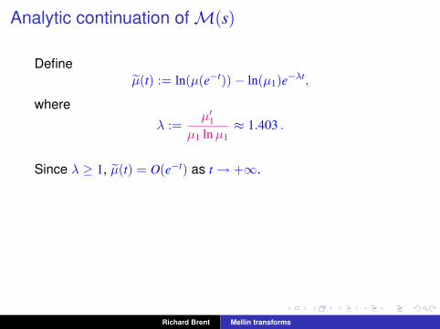
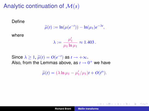
Analytic continuation ofM(s)
Defineµ̃(t) := ln(µ(e−t))− ln(µ1)e−λt,
where
λ :=µ′1
µ1 lnµ1≈ 1.403 .
Since λ ≥ 1, µ̃(t) = O(e−t) as t→ +∞.Also, from the Lemmas above, as t→ 0+ we have
µ̃(t) = (λ lnµ1 − µ′1/µ1)t + O(tα).
Our choice of λ makes the coefficient of t vanish, soµ̃(t) = O(tα).
Richard Brent Mellin transforms
Analytic continuation ofM(s)
Defineµ̃(t) := ln(µ(e−t))− ln(µ1)e−λt,
where
λ :=µ′1
µ1 lnµ1≈ 1.403 .
Since λ ≥ 1, µ̃(t) = O(e−t) as t→ +∞.
Also, from the Lemmas above, as t→ 0+ we have
µ̃(t) = (λ lnµ1 − µ′1/µ1)t + O(tα).
Our choice of λ makes the coefficient of t vanish, soµ̃(t) = O(tα).
Richard Brent Mellin transforms
Analytic continuation ofM(s)
Defineµ̃(t) := ln(µ(e−t))− ln(µ1)e−λt,
where
λ :=µ′1
µ1 lnµ1≈ 1.403 .
Since λ ≥ 1, µ̃(t) = O(e−t) as t→ +∞.Also, from the Lemmas above, as t→ 0+ we have
µ̃(t) = (λ lnµ1 − µ′1/µ1)t + O(tα).
Our choice of λ makes the coefficient of t vanish, soµ̃(t) = O(tα).
Richard Brent Mellin transforms
Analytic continuation ofM(s)
LetM̃(s) :=
∫ ∞0
µ̃(t)ts−1 dt.
Since µ̃(t) = O(tα), the integral converges for <(s) > −α.
Now
M(s) = M̃(s) + ln(µ1)λ−sΓ(s)
gives the analytic continuation ofM(s) into the half-plane
H := {s ∈ C : <(s) > −2 lg(ρ)}.
In H, the only singularities ofM(s) occur at the singularities ofΓ(s), i.e. at s ∈ {0,−1}.
Richard Brent Mellin transforms

Analytic continuation ofM(s)
LetM̃(s) :=
∫ ∞0
µ̃(t)ts−1 dt.
Since µ̃(t) = O(tα), the integral converges for <(s) > −α. Now
M(s) = M̃(s) + ln(µ1)λ−sΓ(s)
gives the analytic continuation ofM(s) into the half-plane
H := {s ∈ C : <(s) > −2 lg(ρ)}.
In H, the only singularities ofM(s) occur at the singularities ofΓ(s), i.e. at s ∈ {0,−1}.
Richard Brent Mellin transforms
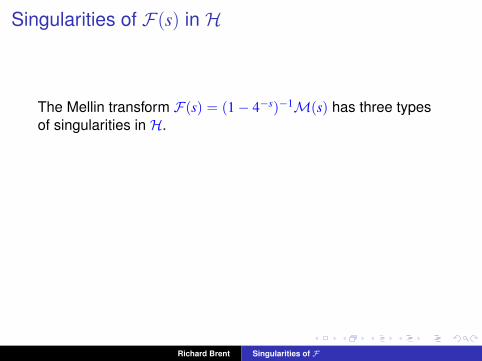
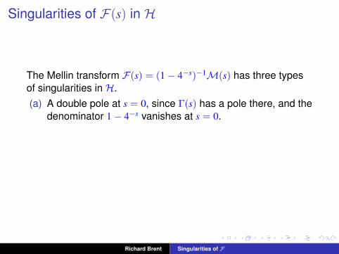
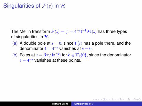
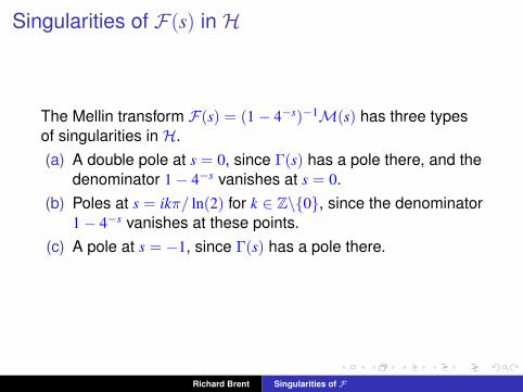
Singularities of F(s) in H
The Mellin transform F(s) = (1− 4−s)−1M(s) has three typesof singularities in H.
(a) A double pole at s = 0, since Γ(s) has a pole there, and thedenominator 1− 4−s vanishes at s = 0.
(b) Poles at s = ikπ/ ln(2) for k ∈ Z\{0}, since the denominator1− 4−s vanishes at these points.
(c) A pole at s = −1, since Γ(s) has a pole there.
Richard Brent Singularities of F
Singularities of F(s) in H
The Mellin transform F(s) = (1− 4−s)−1M(s) has three typesof singularities in H.(a) A double pole at s = 0, since Γ(s) has a pole there, and the
denominator 1− 4−s vanishes at s = 0.
(b) Poles at s = ikπ/ ln(2) for k ∈ Z\{0}, since the denominator1− 4−s vanishes at these points.
(c) A pole at s = −1, since Γ(s) has a pole there.
Richard Brent Singularities of F
Singularities of F(s) in H
The Mellin transform F(s) = (1− 4−s)−1M(s) has three typesof singularities in H.(a) A double pole at s = 0, since Γ(s) has a pole there, and the
denominator 1− 4−s vanishes at s = 0.(b) Poles at s = ikπ/ ln(2) for k ∈ Z\{0}, since the denominator
1− 4−s vanishes at these points.
(c) A pole at s = −1, since Γ(s) has a pole there.
Richard Brent Singularities of F
Singularities of F(s) in H
The Mellin transform F(s) = (1− 4−s)−1M(s) has three typesof singularities in H.(a) A double pole at s = 0, since Γ(s) has a pole there, and the
denominator 1− 4−s vanishes at s = 0.(b) Poles at s = ikπ/ ln(2) for k ∈ Z\{0}, since the denominator
1− 4−s vanishes at these points.(c) A pole at s = −1, since Γ(s) has a pole there.
Richard Brent Singularities of F
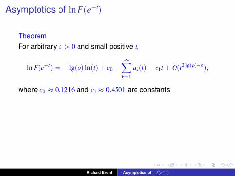
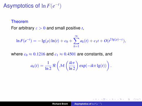
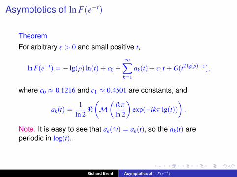
Asymptotics of ln F(e−t)
TheoremFor arbitrary ε > 0 and small positive t,
ln F(e−t) = − lg(ρ) ln(t) + c0 +∞∑
k=1
ak(t) + c1t + O(t2 lg(ρ)−ε),
where c0 ≈ 0.1216 and c1 ≈ 0.4501 are constants, and
ak(t) =1
ln 2<(M(
ikπln 2
)exp(−ikπ lg(t))
).
Note. It is easy to see that ak(4t) = ak(t), so the ak(t) areperiodic in log(t).
Richard Brent Asymptotics of ln F(e−t)
Asymptotics of ln F(e−t)
TheoremFor arbitrary ε > 0 and small positive t,
ln F(e−t) = − lg(ρ) ln(t) + c0 +∞∑
k=1
ak(t) + c1t + O(t2 lg(ρ)−ε),
where c0 ≈ 0.1216 and c1 ≈ 0.4501 are constants
, and
ak(t) =1
ln 2<(M(
ikπln 2
)exp(−ikπ lg(t))
).
Note. It is easy to see that ak(4t) = ak(t), so the ak(t) areperiodic in log(t).
Richard Brent Asymptotics of ln F(e−t)
Asymptotics of ln F(e−t)
TheoremFor arbitrary ε > 0 and small positive t,
ln F(e−t) = − lg(ρ) ln(t) + c0 +∞∑
k=1
ak(t) + c1t + O(t2 lg(ρ)−ε),
where c0 ≈ 0.1216 and c1 ≈ 0.4501 are constants, and
ak(t) =1
ln 2<(M(
ikπln 2
)exp(−ikπ lg(t))
).
Note. It is easy to see that ak(4t) = ak(t), so the ak(t) areperiodic in log(t).
Richard Brent Asymptotics of ln F(e−t)
Asymptotics of ln F(e−t)
TheoremFor arbitrary ε > 0 and small positive t,
ln F(e−t) = − lg(ρ) ln(t) + c0 +∞∑
k=1
ak(t) + c1t + O(t2 lg(ρ)−ε),
where c0 ≈ 0.1216 and c1 ≈ 0.4501 are constants, and
ak(t) =1
ln 2<(M(
ikπln 2
)exp(−ikπ lg(t))
).
Note. It is easy to see that ak(4t) = ak(t), so the ak(t) areperiodic in log(t).
Richard Brent Asymptotics of ln F(e−t)
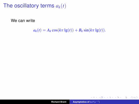
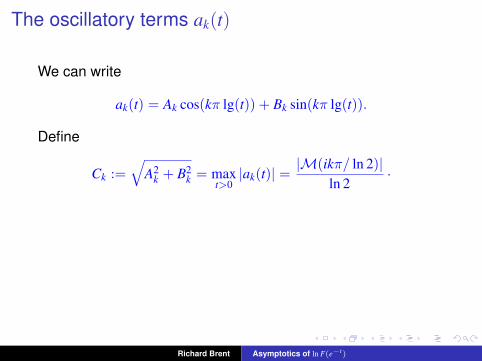
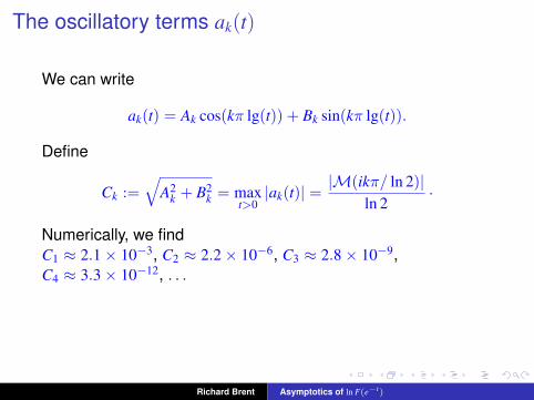
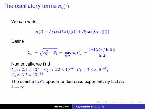
The oscillatory terms ak(t)
We can write
ak(t) = Ak cos(kπ lg(t)) + Bk sin(kπ lg(t)).
Define
Ck :=√
A2k + B2
k = maxt>0|ak(t)| = |M(ikπ/ ln 2)|
ln 2.
Numerically, we findC1 ≈ 2.1× 10⁻³, C2 ≈ 2.2× 10⁻⁶, C3 ≈ 2.8× 10⁻⁹,C4 ≈ 3.3× 10⁻¹², . . .The constants Ck appear to decrease exponentially fast ask→∞.
Richard Brent Asymptotics of ln F(e−t)
The oscillatory terms ak(t)
We can write
ak(t) = Ak cos(kπ lg(t)) + Bk sin(kπ lg(t)).
Define
Ck :=√
A2k + B2
k = maxt>0|ak(t)| = |M(ikπ/ ln 2)|
ln 2.
Numerically, we findC1 ≈ 2.1× 10⁻³, C2 ≈ 2.2× 10⁻⁶, C3 ≈ 2.8× 10⁻⁹,C4 ≈ 3.3× 10⁻¹², . . .
The constants Ck appear to decrease exponentially fast ask→∞.
Richard Brent Asymptotics of ln F(e−t)
The oscillatory terms ak(t)
We can write
ak(t) = Ak cos(kπ lg(t)) + Bk sin(kπ lg(t)).
Define
Ck :=√
A2k + B2
k = maxt>0|ak(t)| = |M(ikπ/ ln 2)|
ln 2.
Numerically, we findC1 ≈ 2.1× 10⁻³, C2 ≈ 2.2× 10⁻⁶, C3 ≈ 2.8× 10⁻⁹,C4 ≈ 3.3× 10⁻¹², . . .The constants Ck appear to decrease exponentially fast ask→∞.
Richard Brent Asymptotics of ln F(e−t)

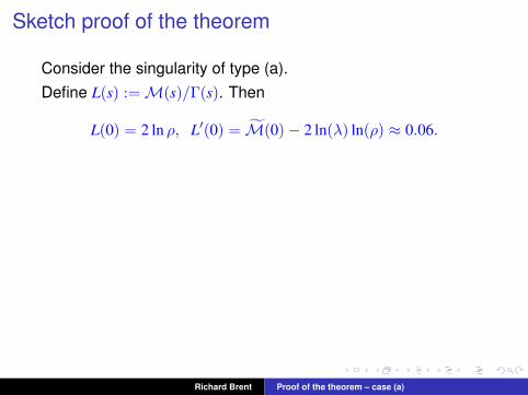
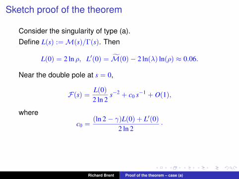
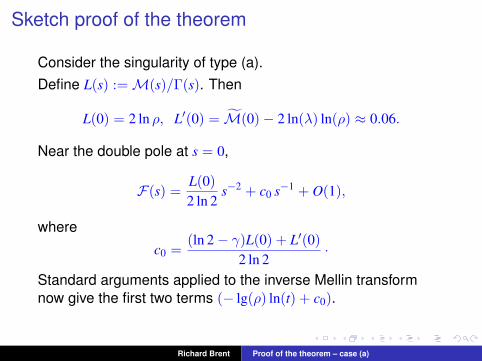
Sketch proof of the theorem
Consider the singularity of type (a).
Define L(s) :=M(s)/Γ(s). Then
L(0) = 2 ln ρ, L′(0) = M̃(0)− 2 ln(λ) ln(ρ) ≈ 0.06.
Near the double pole at s = 0,
F(s) =L(0)2 ln 2
s−2 + c0 s−1 + O(1),
where
c0 =(ln 2− γ)L(0) + L′(0)
2 ln 2.
Standard arguments applied to the inverse Mellin transformnow give the first two terms (− lg(ρ) ln(t) + c0).
Richard Brent Proof of the theorem – case (a)

Sketch proof of the theorem
Consider the singularity of type (a).Define L(s) :=M(s)/Γ(s).
Then
L(0) = 2 ln ρ, L′(0) = M̃(0)− 2 ln(λ) ln(ρ) ≈ 0.06.
Near the double pole at s = 0,
F(s) =L(0)2 ln 2
s−2 + c0 s−1 + O(1),
where
c0 =(ln 2− γ)L(0) + L′(0)
2 ln 2.
Standard arguments applied to the inverse Mellin transformnow give the first two terms (− lg(ρ) ln(t) + c0).
Richard Brent Proof of the theorem – case (a)
Sketch proof of the theorem
Consider the singularity of type (a).Define L(s) :=M(s)/Γ(s). Then
L(0) = 2 ln ρ, L′(0) = M̃(0)− 2 ln(λ) ln(ρ) ≈ 0.06.
Near the double pole at s = 0,
F(s) =L(0)2 ln 2
s−2 + c0 s−1 + O(1),
where
c0 =(ln 2− γ)L(0) + L′(0)
2 ln 2.
Standard arguments applied to the inverse Mellin transformnow give the first two terms (− lg(ρ) ln(t) + c0).
Richard Brent Proof of the theorem – case (a)

Sketch proof continued
Now consider the singularities of type (b).
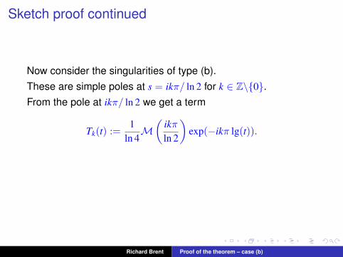
These are simple poles at s = ikπ/ ln 2 for k ∈ Z\{0}.From the pole at ikπ/ ln 2 we get a term
Tk(t) :=1
ln 4M(
ikπln 2
)exp(−ikπ lg(t)).
Combining the terms Tk(t) and T−k(t) for k ≥ 1, the imaginaryparts cancel and we are left with the oscillatory term ak(t).
Richard Brent Proof of the theorem – case (b)

Sketch proof continued
Now consider the singularities of type (b).These are simple poles at s = ikπ/ ln 2 for k ∈ Z\{0}.
From the pole at ikπ/ ln 2 we get a term
Tk(t) :=1
ln 4M(
ikπln 2
)exp(−ikπ lg(t)).
Combining the terms Tk(t) and T−k(t) for k ≥ 1, the imaginaryparts cancel and we are left with the oscillatory term ak(t).
Richard Brent Proof of the theorem – case (b)
Sketch proof continued
Now consider the singularities of type (b).These are simple poles at s = ikπ/ ln 2 for k ∈ Z\{0}.From the pole at ikπ/ ln 2 we get a term
Tk(t) :=1
ln 4M(
ikπln 2
)exp(−ikπ lg(t)).
Combining the terms Tk(t) and T−k(t) for k ≥ 1, the imaginaryparts cancel and we are left with the oscillatory term ak(t).
Richard Brent Proof of the theorem – case (b)

Sketch proof continued
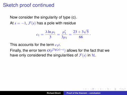
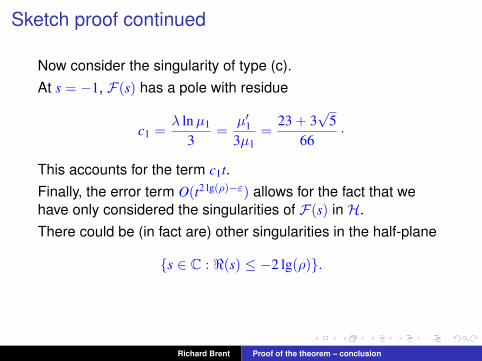
Now consider the singularity of type (c).
At s = −1, F(s) has a pole with residue
c1 =λ lnµ1
3=
µ′13µ1
=23 + 3
√5
66.
This accounts for the term c1t.Finally, the error term O(t2 lg(ρ)−ε) allows for the fact that wehave only considered the singularities of F(s) in H.There could be (in fact are) other singularities in the half-plane
{s ∈ C : <(s) ≤ −2 lg(ρ)}.
Richard Brent Proof of the theorem – conclusion

Sketch proof continued
Now consider the singularity of type (c).At s = −1, F(s) has a pole with residue
c1 =λ lnµ1
3=
µ′13µ1
=23 + 3
√5
66.
This accounts for the term c1t.
Finally, the error term O(t2 lg(ρ)−ε) allows for the fact that wehave only considered the singularities of F(s) in H.There could be (in fact are) other singularities in the half-plane
{s ∈ C : <(s) ≤ −2 lg(ρ)}.
Richard Brent Proof of the theorem – conclusion
Sketch proof continued
Now consider the singularity of type (c).At s = −1, F(s) has a pole with residue
c1 =λ lnµ1
3=
µ′13µ1
=23 + 3
√5
66.
This accounts for the term c1t.Finally, the error term O(t2 lg(ρ)−ε) allows for the fact that wehave only considered the singularities of F(s) in H.
There could be (in fact are) other singularities in the half-plane
{s ∈ C : <(s) ≤ −2 lg(ρ)}.
Richard Brent Proof of the theorem – conclusion
Sketch proof continued
Now consider the singularity of type (c).At s = −1, F(s) has a pole with residue
c1 =λ lnµ1
3=
µ′13µ1
=23 + 3
√5
66.
This accounts for the term c1t.Finally, the error term O(t2 lg(ρ)−ε) allows for the fact that wehave only considered the singularities of F(s) in H.There could be (in fact are) other singularities in the half-plane
{s ∈ C : <(s) ≤ −2 lg(ρ)}.
Richard Brent Proof of the theorem – conclusion

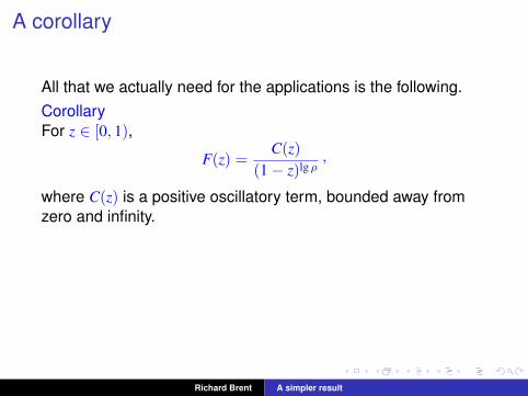
A corollary
All that we actually need for the applications is the following.
CorollaryFor z ∈ [0, 1),
F(z) =C(z)
(1− z)lg ρ,
where C(z) is a positive oscillatory term, bounded away fromzero and infinity.RemarkWe do not need the full machinery of Mellin transforms todeduce the Corollary. Instead we could use the quantitiativeversion of Perron’s theorem due to Coffman (1964).
Richard Brent A simpler result
A corollary
All that we actually need for the applications is the following.CorollaryFor z ∈ [0, 1),
F(z) =C(z)
(1− z)lg ρ,
where C(z) is a positive oscillatory term, bounded away fromzero and infinity.
RemarkWe do not need the full machinery of Mellin transforms todeduce the Corollary. Instead we could use the quantitiativeversion of Perron’s theorem due to Coffman (1964).
Richard Brent A simpler result
A corollary
All that we actually need for the applications is the following.CorollaryFor z ∈ [0, 1),
F(z) =C(z)
(1− z)lg ρ,
where C(z) is a positive oscillatory term, bounded away fromzero and infinity.RemarkWe do not need the full machinery of Mellin transforms todeduce the Corollary. Instead we could use the quantitiativeversion of Perron’s theorem due to Coffman (1964).
Richard Brent A simpler result
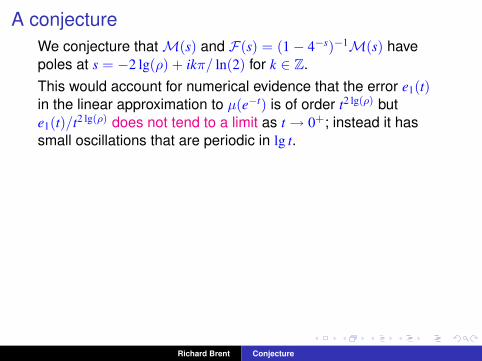
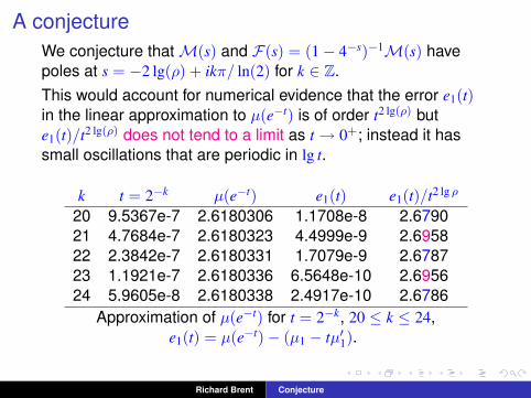
A conjectureWe conjecture thatM(s) and F(s) = (1− 4−s)−1M(s) havepoles at s = −2 lg(ρ) + ikπ/ ln(2) for k ∈ Z.
This would account for numerical evidence that the error e1(t)in the linear approximation to µ(e−t) is of order t2 lg(ρ) bute1(t)/t2 lg(ρ) does not tend to a limit as t→ 0+; instead it hassmall oscillations that are periodic in lg t.
k t = 2−k µ(e−t) e1(t) e1(t)/t2 lg ρ
20 9.5367e-7 2.6180306 1.1708e-8 2.679021 4.7684e-7 2.6180323 4.4999e-9 2.695822 2.3842e-7 2.6180331 1.7079e-9 2.678723 1.1921e-7 2.6180336 6.5648e-10 2.695624 5.9605e-8 2.6180338 2.4917e-10 2.6786
Approximation of µ(e−t) for t = 2−k, 20 ≤ k ≤ 24,e1(t) = µ(e−t)− (µ1 − tµ′1).
Richard Brent Conjecture
A conjectureWe conjecture thatM(s) and F(s) = (1− 4−s)−1M(s) havepoles at s = −2 lg(ρ) + ikπ/ ln(2) for k ∈ Z.This would account for numerical evidence that the error e1(t)in the linear approximation to µ(e−t) is of order t2 lg(ρ) bute1(t)/t2 lg(ρ) does not tend to a limit as t→ 0+; instead it hassmall oscillations that are periodic in lg t.
k t = 2−k µ(e−t) e1(t) e1(t)/t2 lg ρ
20 9.5367e-7 2.6180306 1.1708e-8 2.679021 4.7684e-7 2.6180323 4.4999e-9 2.695822 2.3842e-7 2.6180331 1.7079e-9 2.678723 1.1921e-7 2.6180336 6.5648e-10 2.695624 5.9605e-8 2.6180338 2.4917e-10 2.6786
Approximation of µ(e−t) for t = 2−k, 20 ≤ k ≤ 24,e1(t) = µ(e−t)− (µ1 − tµ′1).
Richard Brent Conjecture
ReferencesB. Adamczewski, Non-converging continued fractions related tothe Stern diatomic sequence, Acta Arith. 142 (2010), 67–78.R. P. Brent, Analysis of the binary Euclidean algorithm, NewDirections and Recent Results in Algorithms and Complexity,Academic Press, New York, 1976, 321–355.R. P. Brent, Twenty years’ analysis of the binary Euclideanalgorithm, Millennial Perspectives in Computer Science . . . ,Palgrave, 2000, 41–53.R. P. Brent, M. Coons and W. Zudilin, Algebraic independenceof Mahler functions via radial asymptotics, IMRN, to appear.P. Bundschuh and K. Väänänen, Transcendence results on thegenerating functions of the characteristic functions of certainself-generating sets, I, Acta Arith. 162 (2014), 273–288.C. V. Coffman, Asymptotic behavior of solutions of ordinarydifference equations, Trans. AMS 110 (1964), 22–51.M. Coons, The transcendence of series related to Stern’sdiatomic sequence, Int. J. Number Theory 6 (2010), 211–217.
Richard Brent References
K. Dilcher and K. Stolarsky, Stern polynomials and double-limitcontinued fractions, Acta Arith. 140 (2009), 119–134.P. Flajolet and R. Sedgewick, Analytic Combinatorics, CUP,2009. Appendix B.7: Mellin transforms.D. E. Knuth, The Art of Computer Programming, Vol. 2:Seminumerical Algorithms (3rd ed.), Addison-Wesley, 1997.G. Maze, Existence of a limiting distribution for the binary GCDalgorithm, J. Discrete Algorithms 5 (2007), 176–186.I. D. Morris, A rigorous version of R. P. Brent’s model for thebinary Euclidean algorithm, arXiv:1409.0729, 2 Sept. 2014.M. A. Stern, Über eine zahlentheoretische Funktion, J. ReineAngew. Math., 55 (1858), 193–220. See also OEIS A002487.B. Vallée, Dynamics of the binary Euclidean algorithm:functional analysis and operators, Algorithmica 22 (1998),660–685.D. Zagier, The Mellin transform and other useful analytictechniques, in E. Zeidler, Quantum Field Theory I . . . ,Springer-Verlag, 2006, 305–323.
Richard Brent References