Embed Size (px)
Citation preview

ASYMPTOTICS OF SOME ULTRA-SPHERICAL POLYNOMIALS
AND THEIR EXTREMA
MAGALI RIBOT
Abstract. Motivated by questions on the preconditioning of spectral meth-ods, and independently of the extensive literature on the approximation of ze-roes of orthogonal polynomials, either by the Sturm method, or by the descentmethod, we develop a stationary phase-like technique for calculating asymp-totics of Legendre polynomials. The difference with the classical stationaryphase method is that the phase is a nonlinear function of the large parameter
and the integration variable, instead of being a product of the large parameterby a function of the integration variable. We then use an implicit functionstheorem for approximating the zeroes of the derivatives of Legendre polyno-mials. This result is used for proving order and consistency of the residualsmoothing scheme [1], [19].
1. Introduction
When we discretize implicitly in time a partial differential equation, we have tosolve a linear system, where the matrix depends on the method used for the spatialdiscretization. Spectral methods are classical methods, but they produce matrices,which are not sparse and difficult to invert; therefore, their numerical efficiencydepends on the introduction of appropriate preconditioners. A preconditioner Pof a matrix M is a matrix, which can be more easily inverted than M and suchthat the condition number of P−1M , that is to say the product of the norm of thematrix P−1M by the norm of its inverse M−1P , is as close to 1 as possible.
In the case of a Laplace — or more generally an elliptic — operator, finite differ-ences or finite elements methods have been proposed for preconditioning spectralmethods in Orszag [13], Haldenwang et al. [11] , Canuto and Quarteroni [3] orDeville and Mund [7, 8].
In [18], Quarteroni and Zampieri investigate the finite element preconditioningof Legendre spectral methods for various boundary conditions; in this article, theyshow numerical evidence of the spectral equivalence between the Legendre spectralmatrix and the finite element matrix. They also apply the preconditioner they pro-pose to domain decomposition methods in the framework of the elasticity problem.
Let us briefly recall that in the one-dimensional situation of a Laplace operator,the coefficients of the mass matrix are defined by the scalar product of the elementsof the basis, whereas the coefficients of the stiffness matrix are given by the scalarproduct of the derivatives of the elements of the basis.
Denote by KS the stiffness matrix associated to a spectral Legendre–Gauss–Lobatto method for −d2/dx2 with Dirichlet boundary conditions, and by KF thestiffness matrix associated to the P1 finite elements method on the nodes of thisspectral method.
Let MS be the mass matrix of the spectral method and let MF be the mass-lumped matrix of the P1 finite elements method constructed on the nodes of the
I would like to thank very warmly Michelle Schatzman for pointing me out this subject andfor many helpful discussions. Many thanks are due to Seymour Parter and David Gottlieb fortheir generous advice and encouragements.
1
2 MAGALI RIBOT
spectral method. We define precisely all these matrices in [19]. We only needhere the coefficients of the diagonal matrix M−1
F MS , which are given later in for-mula (1.6).
Recent results of Parter [15] give the following bounds:
(1.1)1
C≤ Re (KFMSM
−1F U,U)
(KSU,U)≤ |(KFMSM
−1F U,U)|
(KSU,U)≤ C.
Here ( , ) denotes the canonical Hermitian scalar product. These results are basedon [14], which itself builds on Gatteschi’s results [9]. When MF is not mass-lumped,Parter [16] proves an analogous result to estimates (1.1).
The main result of [19] is the spectral equivalence between
M1/2S M
−1/2F KFM
−1/2F M
1/2S
and KS . As a consequence of a result of Parter and Rothman [17], which says thatKF and KS are equivalent, it suffices to prove the spectral equivalence between KF
and
M1/2S M
−1/2F KFM
−1/2F M
1/2S .
This question is motivated by the analysis of the residual smoothing scheme(see [1] and [19]), which allows for fast time integration of the spectral approxima-tion of parabolic equation.
It turns out that when I started working on this question, I was not aware ofParter’s results, and I did not consult the recent literature on orthogonal poly-nomials; instead of using a Sturm method or a descent method, as is done bymost authors in this field, I took the classical integral representation formula forultra-spherical polynomials (4.10.3) from Szego [20], and I applied to this formulaa stationary phase strategy, in a region where the classical expansions cannot beapplied; this method gives an expansion at all orders, with estimates for the errorbound. Let us point out that this is not a classical stationary phase method, sincethe exponential term is a non linear function of the large parameter and of theintegration variable.
Though the present result on preconditioning can be obtained with Parter’smethod, I feel that the treatment presented here of the asymptotics is novel andmore general. Indeed, the detailed calculations given here for derivatives of Le-gendre polynomials could possibly be generalized to other classes of orthogonalpolynomials, such as derivatives of Chebyshev polynomials or more generally to allultra-spherical polynomials.
Let us describe why we need precise asymptotics of the zeroes of the derivatives of
Legendre polynomials to prove the equivalence betweenM1/2S M
−1/2F KFM
−1/2F M
1/2S
and KF . Let us also define precisely our notations.We denote by PN the space of polynomial functions of degree N defined over
[−1, 1]. Let us denote by LN the Legendre polynomial of degree N and let −1 =ξ0 < ξ1 < · · · < ξN−1 < ξN = 1 be the roots of (1 −X2)L′
N ; they are the nodes ofthe spectral method. Let ρk, 0 ≤ k ≤ N be the weights of the quadrature formulaassociated to the nodes ξk; since this is a Gauss-Lobatto formula, we shall have
(1.2) ∀Φ ∈ P2N−1,
∫ 1
−1
Φ(x)dx =
N∑
k=0
Φ(ξk)ρk;
the weights ρk are strictly positive.
ASYMPTOTICS OF SOME ULTRA-SPHERICAL POLYNOMIALS AND THEIR EXTREMA 3
Bernardi and Maday [2] give explicit expressions of the ρk’s:
ρ0 = ρN =2
N(N + 1),
ρk =2
N(N + 1)L2N(ξk)
, 1 ≤ k ≤ N − 1.(1.3)
We define ηk by
(1.4) ηk = Arccos(ξk).
Since we have
−1 = ξ0 < ξ1 < · · · < ξN−1 < ξN = 1,
we infer that
0 = ηN < ηN−1 < · · · < η1 < η0 = π.
Remark 1.1. Since LN is even (resp. odd) when N is even (resp. odd), we seethat
(1.5) ξN−k = −ξk, for 1 ≤ k ≤ N − 1.
The matrices MS and MF are diagonal; we define the diagonal elements ofM−1
F MS as:
(1.6) σk =2ρk
ξk+1 − ξk−1, for 1 ≤ k ≤ N − 1.
We make the convention that σ0 = σN = 0.
Remark 1.2. It has been proved in Lemma 3.1. of [17] and in Lemma 2.1. of [4]that σk is bounded independently of k and N . Precise estimates of σk are availablein Parter’s Theorem 3.1. of [14]. This result is of great importance since thequantities σk appear in several problems related with spectral methods [5, 4].
Define the discrete H1 norm by
‖U‖H1N
= (U∗KFU)1/2
=
(
N−1∑
k=0
|Uk+1 − Uk|2ξk+1 − ξk
)1/2
;
the equivalence between M1/2S M
−1/2F KFM
−1/2F M
1/2S and KF is equivalent to the
existence of a constant C > 0 independent of N such that
C−1‖U‖H1N≤ ‖M−1/2
F M1/2S U‖H1
N≤ C‖U‖H1
N.
Here, as is classical, we had to extend the definition of Uk by letting U0 = UN = 0.
So, let us consider the square of the H1N norm of M
−1/2F M
1/2S U given by
N−1∑
k=0
∣
∣
√σk+1Uk+1 −
√σkUk
∣
∣
2
ξk+1 − ξk.
We first decompose√σk+1 Uk+1 −
√σk Uk as
(1.7)
√σk+1 +
√σk
2
(
Uk+1 − Uk
)
+
√σk+1 −
√σk
2
(
Uk+1 + Uk
)
.
The contribution of the first term of (1.7) in the estimate of the discrete H1 normis
maxk
∣
∣
∣
∣
√σk+1 +
√σk
2
∣
∣
∣
∣
(
N−1∑
k=0
(Uk+1 − Uk)2
ξk+1 − ξk
)1/2
= maxk
∣
∣
∣
∣
√σk+1 +
√σk
2
∣
∣
∣
∣
‖U‖H1
N,
and we use Remark 1.2 to conclude.
4 MAGALI RIBOT
The main result of [19] consists in proving that the contribution of the secondterm of (1.7) can also be estimated in terms of the discrete H1 norm of U . Thisresult can also be deduced from Parter’s article [15]. In a first step, we observe thatdiscrete Holder continuity estimates give
|Uk+1 + Uk|2 ≤(
2 − |ξk| − |ξk+1|)
‖U‖2H1
N.
Thus, we are reduced to estimate
(1.8)
N−1∑
k=0
2 − |ξk| − |ξk+1|ξk+1 − ξk
∣
∣
√σk+1 −
√σk
∣
∣
2.
But σk is bounded from above and from below independently of k, see Remark 1.2;we define
(1.9) µk =2 − |ξk| − |ξk+1|
ξk+1 − ξk
∣
∣
∣
∣
1
σk+1− 1
σk
∣
∣
∣
∣
2
which is algebraically simpler but analytically equivalent to the expression appear-ing in (1.8); according to Lemma 5.7., page 106 of [19], it suffices to show
ΣN =
N−1∑
k=0
µk is bounded independently of N.
Henceforth, we make the convention 1/σ0 = 1/σN = 0.We deduce from symmetry (1.5), formulas (1.3), (1.6) and (1.9) that
µN−k = µk−1, 1 ≤ k ≤ N.
Denote by ⌊r⌋ the largest integer at most equal to the real r. Define N ′ =
⌊
N − 1
2
⌋
;
it suffices to estimate
(1.10) Σ′N =
N ′
∑
k=0
µk
since ΣN ≤ 2Σ′N .
Therefore from the definitions (1.9), (1.6) and (1.3) of µk, σk and ρk, we have toprovide asymptotic expansions for LN and for the zeroes ξk of L′
N ; we start fromclassical integral or asymptotic formulas for Jacobi polynomials that can be foundin the literature.
For the reader’s convenience, it is advisable to consult the fourth edition ofSzego’s book [20], which is the most complete.
We partition the interval {0, · · · , N ′} into three subintervals:
{0, · · · ,K},{K + 1, · · · , ⌊ΛN⌋ − 1} and
{⌊ΛN⌋, · · · , N ′},where K is bounded and will be chosen later, and Λ belongs to the open interval(0, 1/2).
Let us begin with the leftmost region 0 ≤ k ≤ K, where, since K is kept finite,it suffices to find the limit of µk for N tending to infinity. Asymptotics for theLegendre polynomials and their derivatives in this region are available as follows:if N tends to infinity and z is bounded by πK, then
LN
(
cosz
N
)
∼ J0(z)
ASYMPTOTICS OF SOME ULTRA-SPHERICAL POLYNOMIALS AND THEIR EXTREMA 5
where J0 is the classical Bessel function; an analogous statement holds for L′N
(formula (8.1.1) of Szego [20]). If zk denotes the k-th positive zero of the Besselfunction J1, we find for k ≥ 1 [19] :
limN→+∞
µk =z2
k+1 + z2k
64(z2k+1 − z2
k)
∣
∣(z2k+1 − z2
k−1)J20 (zk) − (z2
k+2 − z2k)J2
0 (zk+1)∣
∣
2.
The estimate needed for Theorem 5.8., page 108 of [19] is a direct consequence ofthe above statement. We do not treat the region 0 ≤ k ≤ K in this article, sincewe do not need new asymptotics.
Another result from Szego’s book [20], formula (8.21.14), is: if Λ belongs to(0, 1/2) and πΛN ≤ z ≤ π(1 − Λ)N , we have
P(1/2)N (cos(z/N)) = LN
(
cosz
N
)
= 2ωN,1/2
p−1∑
ν=0
ων,1/21 × 3 · · · × (2ν − 1)
(2N − 1)(2N − 3) · · · (2N − 2ν + 1)
× cos(
(N − ν + 1/2)z/N − (ν + 1/2)π/2)
(2 sin(z/N))ν+1/2+O(N−p−1/2)
(1.11)
where ωN,1/2 is an explicitly known number and the remainder is uniform over theinterval [πΛN, π(1 − Λ)N ]. We also have analogous uniform asymptotics for L′
N ,L′′
N and L′′′N ; therefore, in the rightmost region ⌊ΛN⌋ ≤ k ≤ N ′ and thanks to a
quantitative implicit function theorem, we can find an expansion in terms of k andN of the zero ηk of θ 7→ L′
N (cos θ) which lies in a neighborhood of size O(N−2)about
(1.12) η0,k = π − π/4 + kπ
N + 1/2=
(N − k)π + π/4
N + 1/2;
this result will be proved here as Theorem 2.1 and will lead to an estimate of thequantities σk, ⌊ΛN⌋ ≤ k ≤ N ′ in Corollary 2.4.
There remains to treat the intermediate region, i.e. z between πK and πΛN ; itcorresponds to K ≤ k ≤ ⌊ΛN⌋. This case is not treated in the literature, and wehad to devise the estimates and their proof, using the stationary phase method.
Denote by P(λ)N the ultra-spherical polynomial of degree N over the interval
[−1, 1], i.e. the orthogonal polynomial of degree N relatively to the weight (1 −x2)λ−1/2.
Remark 1.3. The Legendre polynomial LN of degree N is precisely equal to P(1/2)N ,
and as a consequence of (4.7.14) from [20], L′N is equal to P
(3/2)N−1 and L′′
N is equal
to P(5/2)N−2 up to multiplicative constants.
In order to find asymptotics in the intermediate region, we write an integral
representation for P(λ)N :
P(λ)N (x) =
21−2λ
(Γ(λ))2Γ(N + 2λ)
N !
∫ π
0
(
x+ i√
1 − x2 cosϕ)N
sin2λ−1 ϕdϕ.
We apply the principle of the stationary phase method as described in Lemma7.7.3 of Hormander’s book [12], but we cannot apply directly the lemma, since thephase is not equal to a large parameter multiplied by a real function of all theother variables: it is a complex function of the large parameter N and all the othervariables. We set
(1.13) χN = −iN sin(z/N)e−iz/N

6 MAGALI RIBOT
and, for λ such that 2λ− 1 is an even integer, we eventually find polynomials Qν,λ
such that∣
∣
∣
∣
∣
P(λ)N (cos(z/N))
− 2√π
21−2λ
Γ(λ)2Γ(N + 2λ)
N !Re
{
ieizℓ−1∑
ν=λ−1/2
χ−(ν+1/2)N Qν,λ(χN/N)
}∣
∣
∣
∣
∣
≤ C(K,Λ, ℓ, λ)(
N−1 + z−1)ℓ−2λ+1
;
here χ−(ν+1/2)N is the principal determination and C(K,Λ, ℓ, λ) depends only on
its arguments (Theorem 3.14). Finally, we use once again a quantitative implicitfunction theorem to obtain an asymptotic expansion of the zero of L′
N which lies in aneighborhood of size O(1/N2) about π(N −k+1/4)/(N+1/2), for K ≤ k ≤ ⌊ΛN⌋(Corollary 3.17); this asymptotic yields an expansion for σk, K ≤ k ≤ ⌊ΛN⌋ atCorollary 3.19. Hence we obtain in [19] an estimate on the sum of the µk’s forK ≤ k ≤ ⌊ΛN⌋.
The article is organized as follows: in section 2, we compute the asymptoticsof the zeroes in the rightmost region thanks to an implicit functions theorem andwe expand the ratios σk. Section 3, devoted to the intermediate region, is splitinto four sections: in section 3.1, we explain the proof strategy; in section 3.2, weprove a general lemma of stationary or non stationary phase method and we applyit in section 3.3 to obtain expansions of Legendre polynomials; we finally obtainasymptotics of the zeroes of their derivative and of the quantities σk in section 3.4.
2. The region ⌊ΛN⌋ ≤ k ≤ N ′
In order to obtain asymptotics for µk in the index range k ∈ {⌊ΛN⌋, · · · , N ′}in [19] as explained in the introduction, we first need asymptotics for the zeroes of
P(3/2)N = L′
N+1.It is more convenient to state the following theorem in an interval which is
symmetric about N/2:
Theorem 2.1. Define
θ0,k =π/4 + kπ
N + 3/2.
Then for all Λ ∈ (0, 1/2), there exist C, C′ such that for all N ≥ 2 and for all
integer k in {⌊ΛN⌋, · · · , ⌈(1−Λ)N⌉}, there exists a unique zero θk of P(3/2)N (cos θ)
in a ball of radius C′/N2 about θ0,k; moreover the following estimate holds
(2.1)
∣
∣
∣
∣
θk − θ0,k +3
8N2 tan θ0,k− 9
8N3 tan θ0,k
∣
∣
∣
∣
≤ CN−4.
Proof. The idea of the proof is to use the quantitative implicit function theoremgiven in [6]; let us state it here for the reader’s convenience:
Lemma 2.2. Let X and Z be Banach spaces, and let f be a C2 function from aneighborhood U of x0 ∈ X to Z. Let z0 = f(x0). Assume that A = Df(x0) has abounded inverse A−1. Assume that the ball of radius ρ and of center x0 is includedin U . Let
M = sup|ξ|≤ρ
‖A−1D2f(x0 + ξ)‖.
There exist constants a and K given by
a = min(1, (2ρM)−1), K =3aρ
4
ASYMPTOTICS OF SOME ULTRA-SPHERICAL POLYNOMIALS AND THEIR EXTREMA 7
such that if |A−1z0| ≤ K, the equation
f(x) = 0
possesses a unique solution in the ball {|x − x0| ≤ aρ}; moreover, this solutionsatisfies
|x− x0| ≤ 2|A−1z0| and |x− x0 +A−1z0| ≤ 2M |A−1z0|2.
As P(3/2)N has the same parity as N , the set of zeroes of P
(3/2)N is invariant by the
symmetry x 7→ −x, and therefore, at the index level, θk is a zero of P(3/2)N (cos θ) iff
θN−k is a zero of P(3/2)N (cos θ), and moreover, θN−k = π− θk. Therefore, it suffices
to prove the lemma for ΛN ≤ k ≤ N ′.The definition of the binomial coefficients is extended for all x ∈ C and all integer
l ≥ 0 as(
x
l
)
=x(x − 1) · · · (x− l + 1)
l!;
this expression vanishes if x is set equal to 0 or if l is a negative integer. We usethe notation
(2.2) ωN,λ =
(
N + λ− 1
N
)
=Γ(N + λ)
Γ(N + 1)Γ(λ).
We exploit the asymptotics of P(λ)N given as (8.21.14) of [20] for λ = 3/2, 5/2
and 7/2, since we need an estimate of ∂jf/∂θj for j = 0, 1, 2, in order to applyLemma 2.2. We write the three term formula
P(3/2)N (cos θ) =
2ωN,3/2
(2 sin θ)3/2
{
cos(
(N + 3/2)θ − 3π/4)
− 3
2(2N + 1)
cos(
(N + 1/2)θ− 5π/4)
2 sin θ
− 15
8(2N + 1)(2N − 1)
cos(
(N − 1/2)θ− 7π/4)
(2 sin θ)2
}
+O(N−5/2)
(2.3)
which is uniform in θ in [Λ/2, π/2] and in N ; it is then convenient to define
(2.4) f(θ,N) =(2 sin θ)3/2
2ωN,3/2P
(3/2)N (cos θ);
since we seek the unique root θk of f which belongs to a small neighborhood of θ0,k,we will have to calculate f(θ0,k, N), (∂f/∂θ)(θ0,k, N) and to estimate ∂2f/∂θ2 forθ in [θ0,k − rN−2, θ0,k + rN−2]; we will choose r later. We differentiate (2.4) twice,we use formula (4.7.14) from Szego [20], viz.
d
dxP
(λ)N (x) = 2λP
(λ+1)N−1 (x)
and we find
(2.5)∂f
∂θ(θ,N) =
3
2
f(θ,N)
tan θ− 3
√2
ωN,3/2sin5/2θ P
(5/2)N−1 (cos θ),
and
∂2f
∂θ2(θ,N) =
3
4
(
1
tan2 θ− 2
)
f(θ,N) − 12√
2
ωN,3/2cos θ sin3/2θ P
(5/2)N−1 (cos θ)
+15
√2
ωN,3/2sin7/2θ P
(7/2)N−2 (cos θ).
(2.6)
8 MAGALI RIBOT
We first calculate f(θ0,k, N) with the help of formula (2.3) and we find
f(θ0,k, N) =
(−1)k
{
3
4(2N + 1) tan θ0,k− 15
16(2N + 1)(2N − 1) tan θ0,k
}
+O(N−3).(2.7)
We can also evaluate f(θ,N) for |θ − θ0,k| ≤ rN−2: by Taylor expansion,
|cos((N + 3/2)θ− π/4)| ≤ r(N + 3/2)N−2,
and therefore
(2.8) |θ − θ0,k| ≤ rN−2 =⇒ |f(θ)| = (r + 1)O(N−1),
the error term being uniform for k between ⌊ΛN⌋ and N ′.We calculate now ∂f/∂θ at (θ0,k, N): first we substitute the value found at (2.7)
into the first term on the right hand side of (2.5); as θ0,k is bounded away from 0and π, this first term is an O(N−1), uniformly for ΛN ≤ k ≤ N ′. For the second
term of the right hand side of (2.5), we need a two-term expansion of P(5/2)N , namely
P(5/2)N (cos θ) =
2ωN,5/2
(2 sin θ)5/2
(
cos(
(N + 5/2)θ − 5π/4)
− 15
8(N + 3/2)
cos(
(N + 3/2)θ− 7π/4)
sin θ
)
+O(N−1/2).
(2.9)
The error term is uniform on the interval [Λ/2, π/2].We replace N by N − 1 in (2.9) and we observe that
(2.10)6√
2(sin θ)5/2ωN−1,5/2
(2 sin θ)5/2ωN,3/2
=3
2
ωN−1,5/2
ωN,3/2= N,
according to the definition (2.2) of ωN,λ. Furthermore,
cos((N + 3/2)θ0,k − 5π/4) = (−1)k−1
and
cos((N + 1/2)θ0,k − 7π/4) = (−1)k sin(θ0,k).
Thus we find the asymptotic
(2.11) A(k,N) =∂f
∂θ(θ0,k, N) = (−1)k(N + 15/8) +O(N−1).
Now, we choose r:
r =4
3sup{N2|f(θ0,k, N)/A(k,N)| : N ≥ 1,ΛN ≤ k ≤ N ′};
our estimates show that indeed r is bounded.There remains to give an estimate of ∂2f/∂θ2 over the interval [θ0,k−rN−2, θ0,k+
rN−2]. The first term in the right hand side of (2.6) is an O(1/N), thanks to (2.8);the second term in the right hand side of (2.6) is an O(N) in virtue of (2.10) andthe expansion (2.9); the last term in the right hand side of (2.6) is estimated with
the help of the one-term expansion of P(7/2)N given by
P(7/2)N (cos θ) =
2ωN,7/2
(2 sin θ)7/2cos(
(N + 7/2)θ− 7π/4)
+O(N3/2);
but ωN−2,7/2/ωN,3/2 = O(N2) and by a Taylor expansion, cos((N + 3/2)θ− 7π/4)is an O(r/N) on the relevant interval. Therefore, we obtain the estimate
(2.12) |θ − θ0,k| ≤ rN−2 =⇒∣
∣
∣
∣
∂2f
∂θ2(θ,N)
∣
∣
∣
∣
= (r + 1)O(N),
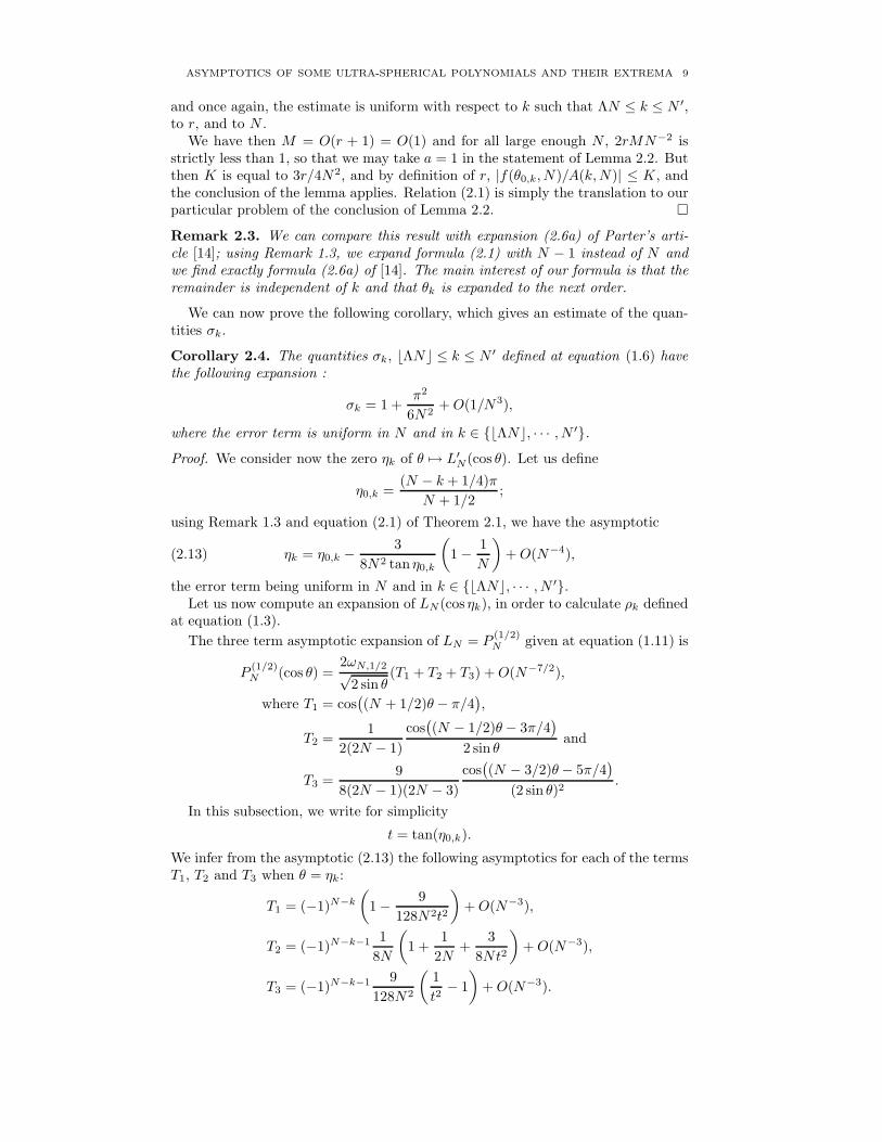
ASYMPTOTICS OF SOME ULTRA-SPHERICAL POLYNOMIALS AND THEIR EXTREMA 9
and once again, the estimate is uniform with respect to k such that ΛN ≤ k ≤ N ′,to r, and to N .
We have then M = O(r + 1) = O(1) and for all large enough N , 2rMN−2 isstrictly less than 1, so that we may take a = 1 in the statement of Lemma 2.2. Butthen K is equal to 3r/4N2, and by definition of r, |f(θ0,k, N)/A(k,N)| ≤ K, andthe conclusion of the lemma applies. Relation (2.1) is simply the translation to ourparticular problem of the conclusion of Lemma 2.2. �
Remark 2.3. We can compare this result with expansion (2.6a) of Parter’s arti-cle [14]; using Remark 1.3, we expand formula (2.1) with N − 1 instead of N andwe find exactly formula (2.6a) of [14]. The main interest of our formula is that theremainder is independent of k and that θk is expanded to the next order.
We can now prove the following corollary, which gives an estimate of the quan-tities σk.
Corollary 2.4. The quantities σk, ⌊ΛN⌋ ≤ k ≤ N ′ defined at equation (1.6) havethe following expansion :
σk = 1 +π2
6N2+O(1/N3),
where the error term is uniform in N and in k ∈ {⌊ΛN⌋, · · · , N ′}.Proof. We consider now the zero ηk of θ 7→ L′
N(cos θ). Let us define
η0,k =(N − k + 1/4)π
N + 1/2;
using Remark 1.3 and equation (2.1) of Theorem 2.1, we have the asymptotic
(2.13) ηk = η0,k − 3
8N2 tan η0,k
(
1 − 1
N
)
+O(N−4),
the error term being uniform in N and in k ∈ {⌊ΛN⌋, · · · , N ′}.Let us now compute an expansion of LN(cos ηk), in order to calculate ρk defined
at equation (1.3).
The three term asymptotic expansion of LN = P(1/2)N given at equation (1.11) is
P(1/2)N (cos θ) =
2ωN,1/2√2 sin θ
(T1 + T2 + T3) +O(N−7/2),
where T1 = cos(
(N + 1/2)θ− π/4)
,
T2 =1
2(2N − 1)
cos(
(N − 1/2)θ− 3π/4)
2 sin θand
T3 =9
8(2N − 1)(2N − 3)
cos(
(N − 3/2)θ− 5π/4)
(2 sin θ)2.
In this subsection, we write for simplicity
t = tan(η0,k).
We infer from the asymptotic (2.13) the following asymptotics for each of the termsT1, T2 and T3 when θ = ηk:
T1 = (−1)N−k
(
1 − 9
128N2t2
)
+O(N−3),
T2 = (−1)N−k−1 1
8N
(
1 +1
2N+
3
8Nt2
)
+O(N−3),
T3 = (−1)N−k−1 9
128N2
(
1
t2− 1
)
+O(N−3).
10 MAGALI RIBOT
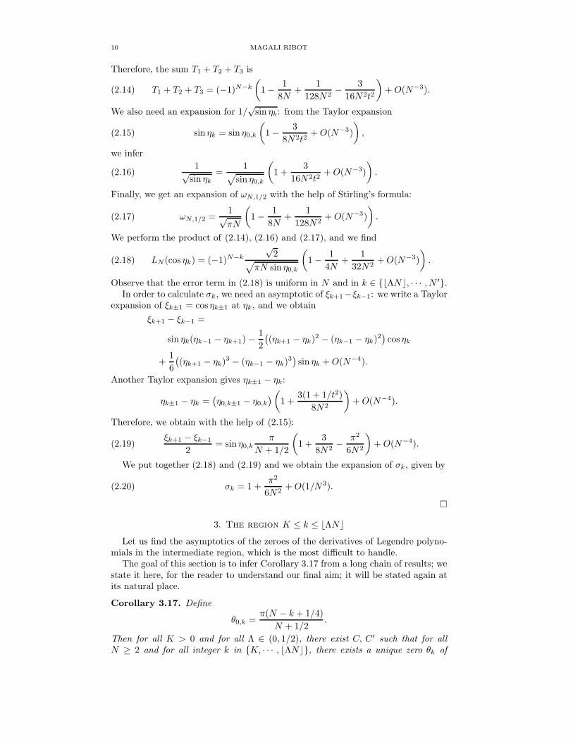
Therefore, the sum T1 + T2 + T3 is
(2.14) T1 + T2 + T3 = (−1)N−k
(
1 − 1
8N+
1
128N2− 3
16N2t2
)
+O(N−3).
We also need an expansion for 1/√
sin ηk: from the Taylor expansion
(2.15) sin ηk = sin η0,k
(
1 − 3
8N2t2+O(N−3)
)
,
we infer
(2.16)1√
sin ηk=
1√
sin η0,k
(
1 +3
16N2t2+O(N−3)
)
.
Finally, we get an expansion of ωN,1/2 with the help of Stirling’s formula:
(2.17) ωN,1/2 =1√πN
(
1 − 1
8N+
1
128N2+O(N−3)
)
.
We perform the product of (2.14), (2.16) and (2.17), and we find
(2.18) LN (cos ηk) = (−1)N−k
√2
√
πN sin η0,k
(
1 − 1
4N+
1
32N2+O(N−3)
)
.
Observe that the error term in (2.18) is uniform in N and in k ∈ {⌊ΛN⌋, · · · , N ′}.In order to calculate σk, we need an asymptotic of ξk+1−ξk−1: we write a Taylor
expansion of ξk±1 = cos ηk±1 at ηk, and we obtain
ξk+1 − ξk−1 =
sin ηk(ηk−1 − ηk+1) −1
2
(
(ηk+1 − ηk)2 − (ηk−1 − ηk)2)
cos ηk
+1
6
(
(ηk+1 − ηk)3 − (ηk−1 − ηk)3)
sin ηk +O(N−4).
Another Taylor expansion gives ηk±1 − ηk:
ηk±1 − ηk =(
η0,k±1 − η0,k
)
(
1 +3(1 + 1/t2)
8N2
)
+O(N−4).
Therefore, we obtain with the help of (2.15):
(2.19)ξk+1 − ξk−1
2= sin η0,k
π
N + 1/2
(
1 +3
8N2− π2
6N2
)
+O(N−4).
We put together (2.18) and (2.19) and we obtain the expansion of σk, given by
(2.20) σk = 1 +π2
6N2+O(1/N3).
�
3. The region K ≤ k ≤ ⌊ΛN⌋Let us find the asymptotics of the zeroes of the derivatives of Legendre polyno-
mials in the intermediate region, which is the most difficult to handle.The goal of this section is to infer Corollary 3.17 from a long chain of results; we
state it here, for the reader to understand our final aim; it will be stated again atits natural place.
Corollary 3.17. Define
θ0,k =π(N − k + 1/4)
N + 1/2.
Then for all K > 0 and for all Λ ∈ (0, 1/2), there exist C, C′ such that for allN ≥ 2 and for all integer k in {K, · · · , ⌊ΛN⌋}, there exists a unique zero θk of
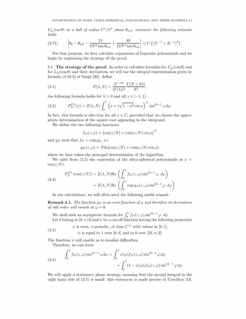
ASYMPTOTICS OF SOME ULTRA-SPHERICAL POLYNOMIALS AND THEIR EXTREMA 11
L′N(cos θ) in a ball of radius C′/N2 about θ0,k; moreover the following estimate
holds
(3.71)
∣
∣
∣
∣
θk − θ0,k − 13
8N2 tan θ0,k+
49
12N3 tan θ0,k
∣
∣
∣
∣
≤ C(
(N−1 +K−1)4)
.
For that purpose, we first calculate expansions of Legendre polynomials and webegin by explaining the strategy of the proof.
3.1. The strategy of the proof. In order to calculate formulas for L′N(cos θ) and
for LN(cos θ) and their derivatives, we will use the integral representation given byformula (4.10.3) of Szego [20]: define
(3.1) Z(λ,N) =21−2λ
(Γ(λ))2Γ(N + 2λ)
N !,
the following formula holds for λ > 0 and all x ∈ [−1, 1]:
(3.2) P(λ)N (x) = Z(λ,N)
∫ π
0
(
x+ i√
1 − x2 cosϕ)N
sin2λ−1 ϕdϕ.
In fact, this formula is also true for all x ∈ C, provided that we choose the appro-priate determination of the square root appearing in the integrand.
We define the two following functions:
fN (z, ϕ) =(
cos(z/N) + i sin(z/N) cosϕ)N
and gN such that fN = exp gN , i.e.
gN(z, ϕ) = N ln(
cos(z/N) + i sin(z/N) cosϕ)
where we have taken the principal determination of the logarithm.We infer from (3.2) the expression of the ultra-spherical polynomials at x =
cos(z/N):
P(λ)N (cos(z/N)) = Z(λ,N)Re
(∫ π
0
fN (z, ϕ) sin2λ−1 ϕ dϕ
)
= Z(λ,N)Re
(∫ π
0
exp gN (z, ϕ) sin2λ−1 ϕ dϕ
)(3.3)
In our calculations, we will often need the following useful remark:
Remark 3.1. The function gN is an even function of ϕ and therefore its derivativesof odd order will vanish at ϕ = 0.
We shall seek an asymptotic formula for∫ π
0fN (z, ϕ) sin2λ−1 ϕ dϕ.
Let δ belong to [0, π/4[ and ψ be a cut-off function having the following properties
(3.4)ψ is even, π-periodic, of class C∞ with values in [0, 1],
ψ is equal to 1 over [0, δ] and to 0 over [2δ, π/2].
The function ψ will enable us to localize difficulties.Therefore, we can write
∫ π
0
fN (z, ϕ) sin2λ−1 ϕdϕ =
∫ π
0
ψ(ϕ)fN (z, ϕ) sin2λ−1 ϕdϕ
+
∫ π
0
(1 − ψ(ϕ))fN (z, ϕ) sin2λ−1 ϕdϕ.
(3.5)
We will apply a stationary phase strategy, meaning that the second integral in theright hand side of (3.5) is small: this statement is made precise at Corollary 3.6.
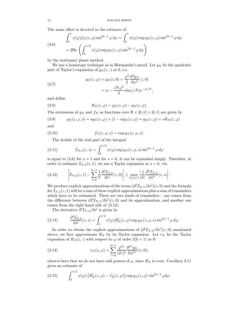
12 MAGALI RIBOT
The main effort is devoted to the estimate of∫ π
0
ψ(ϕ)fN (z, ϕ) sin2λ−1 ϕdϕ =
∫ π
0
ψ(ϕ) exp gN(z, ϕ) sin2λ−1 ϕdϕ
= 2Re
(
∫ π/2
0
ψ(ϕ) exp gN (z, ϕ) sin2λ−1 ϕdϕ
)(3.6)
by the stationary phase method.We use a homotopy technique as in Hormander’s proof. Let qN be the quadratic
part of Taylor’s expansion of gN (z, ·) at 0, i.e.
qN (z, ϕ) = gN(z, 0) +ϕ2
2
∂2gN
∂ϕ2(z, 0)
= iz − iNϕ2
2sin(z/N)e−iz/N ,
(3.7)
and define
(3.8) RN (z, ϕ) = gN (z, ϕ) − qN (z, ϕ).
The extensions of gN and fN as functions over R × [0, π] × [0, 1] are given by
(3.9) gN(z, ϕ, s) = sgN(z, ϕ) + (1 − s)qN (z, ϕ) = qN (z, ϕ) + sRN (z, ϕ)
and
(3.10) fN (z, ϕ, s) = exp gN (z, ϕ, s).
The double of the real part of the integral
(3.11) IN,λ(z, s) =
∫ π/2
0
ψ(ϕ) exp gN(z, ϕ, s) sin2λ−1 ϕdϕ
is equal to (3.6) for s = 1 and for s = 0, it can be expanded simply. Therefore, inorder to estimate IN,λ(z, 1), we use a Taylor expansion at s = 0, viz.
(3.12)
∣
∣
∣
∣
∣
IN,λ(z, 1) −k−1∑
l=0
1
l!
∂lIN,λ
∂sl(z, 0)
∣
∣
∣
∣
∣
≤ max0≤s≤1
∣
∣
∣
∣
1
k!
∂kIN,λ
∂sk(z, s)
∣
∣
∣
∣
.
We produce explicit approximations of the terms (∂lIN,λ/∂sl)(z, 0) and the formula
for IN,λ(z, 1) will be a sum of these explicit approximations plus a sum of remainderswhich have to be estimated. There are two kinds of remainders : one comes fromthe difference between (∂lIN,λ/∂s
l)(z, 0) and its approximation, and another onecomes from the right hand side of (3.12).
The derivative ∂lIN,λ/∂sl is given by
(3.13)∂lIN,λ
∂sl(z, s) =
∫ π/2
0
ψ(ϕ)RlN (z, ϕ) exp gN(z, ϕ, s) sin2λ−1 ϕdϕ.
In order to obtain the explicit approximations of (∂lIN,λ/∂sl)(z, 0) mentioned
above, we first approximate RN by its Taylor expansion. Let rN be the Taylorexpansion of RN (z, ·) with respect to ϕ of order 2(k + 1) at 0:
(3.14) rN (z, ϕ) =
k+1∑
γ=2
ϕ2γ
(2γ)!
∂2γgN
∂ϕ2γ(z, 0);
observe here that we do not have odd powers of ϕ, since RN is even. Corollary 3.11gives an estimate of
(3.15)
∫ π/2
0
ψ(ϕ)(
RlN (z, ϕ) − rl
N (z, ϕ))
exp qN (z, ϕ) sin2λ−1 ϕdϕ.
ASYMPTOTICS OF SOME ULTRA-SPHERICAL POLYNOMIALS AND THEIR EXTREMA 13
Then, the usable explicit approximations will be calculated using Lemma 7.7.3 ofHormander [12] for the following integrals :
∫ π/2
0
ψ(ϕ)rlN (z, ϕ) exp gN (z, ϕ, s) sin2λ−1 ϕdϕ,
which is done at Corollary 3.13.Finally, we estimate ∂kIN,λ/∂s
k, which is the main part of the right hand sideof equation (3.12), at Corollary 3.9.
The usable algebraic expressions of the terms which appear in asymptotics of
P(λ)N are given first in general form at Theorem 3.14 for 2λ−1 an even integer, and
explicit results for λ = 1/2, 3/2, 5/2 and 7/2 are given at Corollary 3.15.
3.2. A general lemma of stationary and non-stationary methods. We showa general lemma to help proving all the estimates explained in section 3.1.
We need several preliminary technical results. First we estimate exp(gN (z, ϕ, s)).
Lemma 3.2. For all N ≥ 2, for all ϕ ∈ [0, π], for all z ∈ R+ and for all s ∈ [0, 1],
| exp(gN(z, ϕ, s))| ≤ 1.
Proof. It suffices to check Re gN (z, ϕ, s) ≤ 0 which is true provided that Re gN (z, ϕ)and Re qN (z, ϕ) are less than or equal to 0.
The real part of gN is N ln(
1 − sin2(z/N) sin2 ϕ)
/2 which has the required sign.
The real part of qN is −Nϕ2 sin2(z/N)/2 which is also less than or equal to 0. �
Differentiating composite functions can be done with the help of Faa di Bruno’sformula, see for instance Lemma II.2.8 of Hairer [10].
For m ∈ N, let C(m) be the set of multi-indices γ = (γ1, γ2, · · · ) ∈ NN∗
such thatγ1 ≥ γ2 ≥ · · · and such that
∑
i∈Nγi = m. Therefore γi vanishes beyond a certain
rank; we denote by l(γ) the largest integer i such that γi ≥ 1 and we observe thatl(γ) ≤ m. For instance, if we only write the non zero terms of each γ, C(3) is equalto {(3), (2, 1), (1, 1, 1)}.
Faa di Bruno’s formula states that there exist integer constants C(γ,m) suchthat
(3.16)dm
dxmA ◦B =
∑
γ∈C(m)
C(γ,m)(A(l(γ)) ◦B)
l(γ)∏
j=1
B(γj).
Here, A and B are functions of one real variable. In consequence, if we takeA(x) = xk, with k ∈ Z, we can calculate for any function B the derivatives ofBk :
(3.17)dm
dxmBk =
∑
γ∈C(m)
C(γ,m)
(
k
l(γ)
)
l(γ)!Bk−l(γ)
l(γ)∏
j=1
B(γj).
Let us estimate now the derivatives of (∂gN/∂ϕ)−1, which will arise later whenwe will perform several integrations by part, and let us also estimate the derivativesof gN .
Lemma 3.3. For all k ∈ N, for all α > 0, there exists C > 0 such that for allN ≥ 2, for all ϕ ∈ (0, π − α] and for all z ∈ [πK, πΛN ], the following estimateshold
(3.18)
∣
∣
∣
∣
∂k
∂ϕk
(
1
∂gN/∂ϕ
)
(z, ϕ)
∣
∣
∣
∣
≤ C
ϕk+1(N−1 + z−1)

14 MAGALI RIBOT
and
(3.19)
∣
∣
∣
∣
∂k+1gN
∂ϕk+1(z, ϕ)
∣
∣
∣
∣
≤ Cz.
Proof. Write
(3.20)ν(ϕ) = sinϕ (as in numerator) and
dN (z, ϕ) =(
cos(z/N) + i sin(z/N) cosϕ)
(as in denominator).
Then the first derivative of gN and its inverse are
(3.21)∂gN
∂ϕ(z, ϕ) = −iN sin(z/N)
ν(ϕ)
dN(z, ϕ)
and
(3.22)1
∂gN/∂ϕ(z, ϕ) =
i
N sin(z/N)
dN (z, ϕ)
ν(ϕ).
Leibniz formula gives
(3.23)∂k
∂ϕk
(
1
∂gN/∂ϕ
)
=i
N sin(z/N)
k∑
m=0
(
k
m
)
∂k−mdN
∂ϕk−m
∂m
∂ϕm
(
1
ν
)
.
The successive derivatives of 1/ν are computed using (3.17) for k = −1; up toarithmetic constants, the terms we find in (3.23) are of the form
(3.24)i
N sin(z/N)
∂k−mdN
∂ϕk−mν−1−l(γ)
l(γ)∏
j=1
∂γjν
∂ϕγj;
we substitute the expressions of the derivatives
(3.25)∂jdN
∂ϕj(z, ϕ) = i sin(z/N) cos (ϕ+ jπ/2) , for all j ≥ 1
and
(3.26)∂nν
∂ϕn(ϕ) = sin (ϕ+ nπ/2)
into (3.24): for m = k, the expressions (3.24) are equal to
i(cos(z/N) + i sin(z/N) cosϕ)
N sin(z/N)
1
sin1+l(γ) ϕ
l(γ)∏
j=1
sin(ϕ+ γjπ/2)
which can be estimated by C/(zϕk+1).For m ≤ k − 1, the terms (3.24) are of the form
− 1
Ncos(ϕ+ (k −m)π/2)
1
sin1+l(γ) ϕ
l(γ)∏
j=1
sin(ϕ+ γjπ/2)
which can be estimated by C/(Nϕk+1), proving thus (3.18).Similarly, we write a Leibniz formula for ∂k+1gN/∂ϕ
k+1:
(3.27)∂k+1gN
∂ϕk+1(z, ϕ) = −iN sin(z/N)
k∑
m=0
(
k
m
)
∂k−mν
∂ϕk−m(ϕ)
∂m
∂ϕm
(
1
dN
)
(z, ϕ).
ASYMPTOTICS OF SOME ULTRA-SPHERICAL POLYNOMIALS AND THEIR EXTREMA 15
We use formula (3.17) with k = −1, i.e.
∂m
∂ϕm
(
1
dN
)
(z, ϕ) =∑
γ∈C(m)
C(γ,m)(−1)l(γ)l(γ)!d−1−l(γ)N (z, ϕ)
×l(γ)∏
j=1
∂γjdN
∂ϕγj(z, ϕ);
(3.28)
up to arithmetic constants, we substitute the values (3.25) and (3.26) of the deriva-tives of dN and ν and for k ≥ 1, Leibniz formula implies that the terms of thesum (3.27) are of the following form
− iN sin(z/N) sin(ϕ+ (k −m)π/2)(i sin z/N)l(γ)
(cos z/N + i sin z/N cosϕ)1+l(γ)
×l(γ)∏
j=1
cos(ϕ+ γjπ/2).
(3.29)
It is plain that the modulus of (3.29) is at most equal to N |sin z/N | and theconclusion of the lemma is clear. �
The technical lemma 3.5 will be used many times in the foregoing estimates; itdepends on the preliminary lemma 3.4.
Let p ∈ N and b ∈ (0, π). Let u be a function of class Cp over [πK,+∞)× [0, b];assume that there exist a real c ≥ 2p and a real l ≥ 0 such that the following norm
(3.30) ‖u‖p,c,l = max0≤i≤p
maxN∈N
maxϕ∈(0,b]
z∈[πK,πΛN ]
z−lϕ−c+i
∣
∣
∣
∣
∂iu
∂ϕi(z, ϕ)
∣
∣
∣
∣
is finite. We define by induction
(3.31)
U0 = u,
Um+1 =∂
∂ϕ
(
Um
∂gN/∂ϕ
)
for all m ∈ {0, · · · , p− 1}.
We need to estimate the derivatives of the functions (3.31), since they will appearin the integration by parts which will be performed in the stationary and nonstationary phase methods.
Lemma 3.4. Let u be a function of class Cp over [πK,+∞) × [0, b]; assume thatthere exist c ≥ 2p and l ≥ 0 such that ‖u‖p,c,l < +∞. Then, there exists C > 0
such that for all N ≥ 2, for all m ∈ {0, · · · , p}, for all q ∈ {0, · · · , p −m}, for allϕ ∈ [0, b] and for all z ∈ [πK, πΛN ],
(3.32)
∣
∣
∣
∣
∂q
∂ϕqUm(z, ϕ)
∣
∣
∣
∣
≤ C ‖u‖q+m,c,l (N−1 + z−1)m−lϕc−q−2m.
Proof. Let us prove this lemma by induction on m. We have
∂qU0
∂ϕq(z, ϕ) =
∂qu
∂ϕq(z, ϕ)
and thus using the hypothesis made on ‖u‖p,c,l, we infer that∣
∣
∣
∣
∂qU0
∂ϕq(z, ϕ)
∣
∣
∣
∣
≤ ‖u‖q,c,l zlϕc−q ≤ C ‖u‖q,c,l (N
−1 + z−1)−lϕc−q.
Assuming that estimate (3.32) is proved for m, we use definition (3.31) and Leibnizformula:
16 MAGALI RIBOT
∂qUm+1
∂ϕq=
q+1∑
s=0
(
q + 1
s
)
∂q+1−sUm
∂ϕq+1−s
∂s
∂ϕs
(
1
∂gN/∂ϕ
)
.
Using the induction hypothesis and Lemma 3.3,∣
∣
∣
∣
∣
∂q+1−sUm
∂ϕq+1−s(z, ϕ)
∂s
∂ϕs
(
1
∂gN/∂ϕ
)
(z, ϕ)
∣
∣
∣
∣
∣
≤ C ‖u‖q+m+1−s,c,l (N−1 + z−1)m+1−lϕc−q−2−2m
≤ C ‖u‖q+m+1,c,l (N−1 + z−1)m+1−lϕc−q−2(m+1),
and the proof of Lemma 3.4 is complete. �
Here is our general lemma:
Lemma 3.5. Let k ∈ N∗ and b ∈ [0, π). Take u in C∞0 ([πK,+∞)× [0, b]); assume
that there exist l ≥ 0 and c ≥ 2(k + l) such that ‖u‖k+l,c,l is finite. Then there
exists C such that for all N ≥ 2 and all z ∈ [πK, πΛN ],
(3.33) maxs∈[0,1]
∣
∣
∣
∣
∣
∫ b
0
u(z, ϕ) exp gN (z, ϕ, s) dϕ
∣
∣
∣
∣
∣
≤ C ‖u‖k+l,c,l (N−1 + z−1)k.
Proof. Thanks to several integrations by part and using definition (3.31), we canwrite the integral appearing in the left hand side of (3.33) as
∫ b
0
u(z, ϕ) exp gN (z, ϕ, s) dϕ =
k+l−1∑
m=0
[
(−1)m
∂gN/∂ϕUm(z, ϕ) exp gN (z, ϕ, s)
]b
0
+ (−1)k+l
∫ b
0
Uk+l(z, ϕ) exp gN(z, ϕ, s) dϕ.
(3.34)
Since u is equal to 0 in a neighborhood of ϕ = b, for all m ∈ {0, · · · , k + l− 1}, forall z in [πK, πΛN ], Um(z, b) vanishes and thus all the integrated terms at ϕ = bdisappear:
∫ b
0
u(z, ϕ) exp gN(z, ϕ, s) dϕ =
k+l−1∑
m=0
(−1)m Um
∂gN/∂ϕ(z, 0) expgN (z, 0, s)
+ (−1)k+l
∫ b
0
Uk+l(z, ϕ) exp gN (z, ϕ, s) dϕ.
(3.35)
Thanks to Lemmas 3.3 and 3.4, we can estimate all these terms.Lemma 3.3 with k = 0 and Lemma 3.4 with q = 0 give for m in {0, · · · , k+ l−1},
in the neighborhood of ϕ = 0,
Um
∂gN/∂ϕ(z, ϕ) = O(1)(N−1 + z−1)m−l+1ϕc−2m−1
where O(1) is bounded independently of ϕ ∈ [0, b], z ∈ [πK, πΛN ], N ≥ 2 and offinite l and m. Since c ≥ 2(k + l) > 2m+ 1, we obtain
[
Um/(∂gN/∂ϕ)]
(z, 0) = 0.Moreover, exp gN (z, 0, s) = exp(iz) and thus equation (3.35) becomes
∫ b
0
u(z, ϕ) exp gN(z, ϕ, s) dϕ
= (−1)k+l
∫ b
0
Uk+l(z, ϕ) exp gN (z, ϕ, s) dϕ.
ASYMPTOTICS OF SOME ULTRA-SPHERICAL POLYNOMIALS AND THEIR EXTREMA 17
Thanks to Lemma 3.2 and Lemma 3.4 with m = k + l and q = 0, we obtainestimate (3.33). �
3.3. Asymptotics of Legendre polynomials. Now that Lemma 3.5 is proved,we can estimate the integrals displayed in section 3.1.
First, a straightforward corollary of Lemma 3.5 shows that the second integralof the right hand side of (3.5) is small.
Corollary 3.6. Let ψ satisfy conditions (3.4). For all positive integer k and forall λ > 0, there exists C such that for all N ≥ 2 and for all z in [πK, πΛN ], thefollowing estimate holds:
(3.36)
∣
∣
∣
∣
∫ π
0
(1 − ψ(ϕ)) exp gN(z, ϕ) sin2λ−1 ϕdϕ
∣
∣
∣
∣
≤ C(N−1 + z−1)k.
Proof. We use Lemma 3.5 with u(z, ϕ) = (1 − ψ(ϕ)) sin2λ−1 ϕ and b = π − δ/2.The function u and its derivatives vanish in a neighborhood of ϕ = b and in theneighborhood [−δ, δ] of 0; if we set l = 0 and c = 2k, ‖u‖k,2k,0 is finite. We inferfrom Lemma 3.5 that
∣
∣
∣
∣
∫ π
0
(1 − ψ(ϕ)) exp gN(z, ϕ, 1) sin2λ−1 ϕdϕ
∣
∣
∣
∣
=
∣
∣
∣
∣
∣
∫ π− δ2
0
(1 − ψ(ϕ)) exp gN(z, ϕ, 1) sin2λ−1 ϕdϕ
∣
∣
∣
∣
∣
≤ C ‖u‖k,2k,0 (N−1 + z−1)k,
where C depends only on k, which is estimate (3.36). �
In order to apply Lemma 3.5 to the remainder defined by equation (3.12), weneed to estimate the derivatives of the powers of RN , defined at equation (3.8).
Lemma 3.7. For all k ∈ N∗ and m ∈ N, there exists C > 0 such that for allN ≥ 2, for all z ∈ [πK, πΛN ] and for all ϕ ∈ [0, π/2],
(3.37)
∣
∣
∣
∣
∂mRkN
∂ϕm(z, ϕ)
∣
∣
∣
∣
≤ Czk min(1, ϕ4k−m).
Proof. For k = 1 and m ≤ 3, Taylor’s integral formula gives
∂mRN (z, ϕ)
∂ϕm=
∫ ϕ
0
∂4gN
∂ϕ4(z, ϕ′)
(ϕ− ϕ′)3−m
(3 −m)!dϕ′,
and for m ≥ 4,∂mRN
∂ϕm=∂mgN
∂ϕm.
We infer immediately from these relations and the parity of RN with respect to ϕthe estimates
(3.38)
|RN (z, ϕ)| ≤ Cϕ4z,∣
∣
∣
∣
∂RN
∂ϕ(z, ϕ)
∣
∣
∣
∣
≤ Cϕ3z,
∣
∣
∣
∣
∂2RN
∂ϕ2(z, ϕ)
∣
∣
∣
∣
≤ Cϕ2z,
∣
∣
∣
∣
∂mRN
∂ϕm(z, ϕ)
∣
∣
∣
∣
≤ Cϕz for m ≥ 3, m odd,
∣
∣
∣
∣
∂mRN
∂ϕm(z, ϕ)
∣
∣
∣
∣
≤ Cz for m ≥ 4, m even.

18 MAGALI RIBOT
Using Faa di Bruno’s formula (3.17), we obtain
(3.39)∂mRk
N
∂ϕm(z, ϕ) =
∑
γ∈C(m)
C(γ,m)
(
k
l(γ)
)
l(γ)!Rk−l(γ)N (z, ϕ)
l(γ)∏
j=1
∂γjRN
∂ϕγj(z, ϕ).
Let us denote by ν1 the number of indices j ∈ {1, · · · , l(γ)} such that γj = 1, byν2 the number of indices j ∈ {1, · · · , l(γ)} such that γj = 2; νo is the number ofindices j such that γj ≥ 3 is odd and νe is the number of indices such that γj ≥ 4is even.
Thus, we have the following two relations:
ν1 + ν2 + νo + νe = l(γ)(3.40)
and
m = γ1 + · · · + γl(γ) ≥ ν1 + 2ν2 + 3νo + 4νe.(3.41)
We infer from equation (3.38) the estimate∣
∣
∣
∣
∣
∣
Rk−l(γ)N (z, ϕ)
l(γ)∏
j=1
∂γjRN
∂ϕγj(z, ϕ)
∣
∣
∣
∣
∣
∣
≤ Czαϕ4k−4l(γ)+3ν1+2ν2+νo
where α = k − l(γ) + ν1 + ν2 + νo + νe, and from equation (3.40), we infer theestimate∣
∣
∣
∣
∣
∣
Rk−l(γ)N (z, ϕ)
l(γ)∏
j=1
∂γjRN
∂ϕγj(z, ϕ)
∣
∣
∣
∣
∣
∣
≤ Czkϕ4k−4l(γ)+3ν1+2ν2+νo .
Equations (3.40) and (3.41) lead to
4k − 4l(γ) + 3ν1 + 2ν2 + νo = 4k − ν1 − 2ν2 − 3νo − 4νe ≥ 4k −m
and the expression 4k−4l(γ)+3ν1+2ν2+νo is also non negative since l(γ) belongsto {0, · · · , k}; this completes the proof of estimate (3.37). �
We deduce easily an analogous lemma for the derivatives of the powers of rN ,defined at equation (3.14).
Lemma 3.8. For all k ∈ N∗ and m ∈ N, there exists C > 0 such that for allN ≥ 2, for all z ∈ [πK, πΛN ] and for all ϕ ∈ [0, π/2],
(3.42)
∣
∣
∣
∣
∂mrkN
∂ϕm(z, ϕ)
∣
∣
∣
∣
≤ Czk min(1, ϕ4k−m).
Proof. The estimates for ∂mrN/∂ϕm are analogous to the estimates (3.38) for
∂mRN/∂ϕm and consequently the estimate for ∂mrk
N/∂ϕm is the same as esti-
mate (3.37) for ∂mRkN/∂ϕ
m. �
Recall that IN,λ has been defined at equation (3.11). The following corollarygives estimates of its derivatives.
Corollary 3.9. For all integer k ≥ 1 and all λ ≥ 1/2, there exists C such that forall N ≥ 2 and for all z in [πK, πΛN ] ,
(3.43) maxs∈[0,1]
∣
∣
∣
∣
∂kIN,λ
∂sk(z, s)
∣
∣
∣
∣
≤ C(N−1 + z−1)k.
ASYMPTOTICS OF SOME ULTRA-SPHERICAL POLYNOMIALS AND THEIR EXTREMA 19
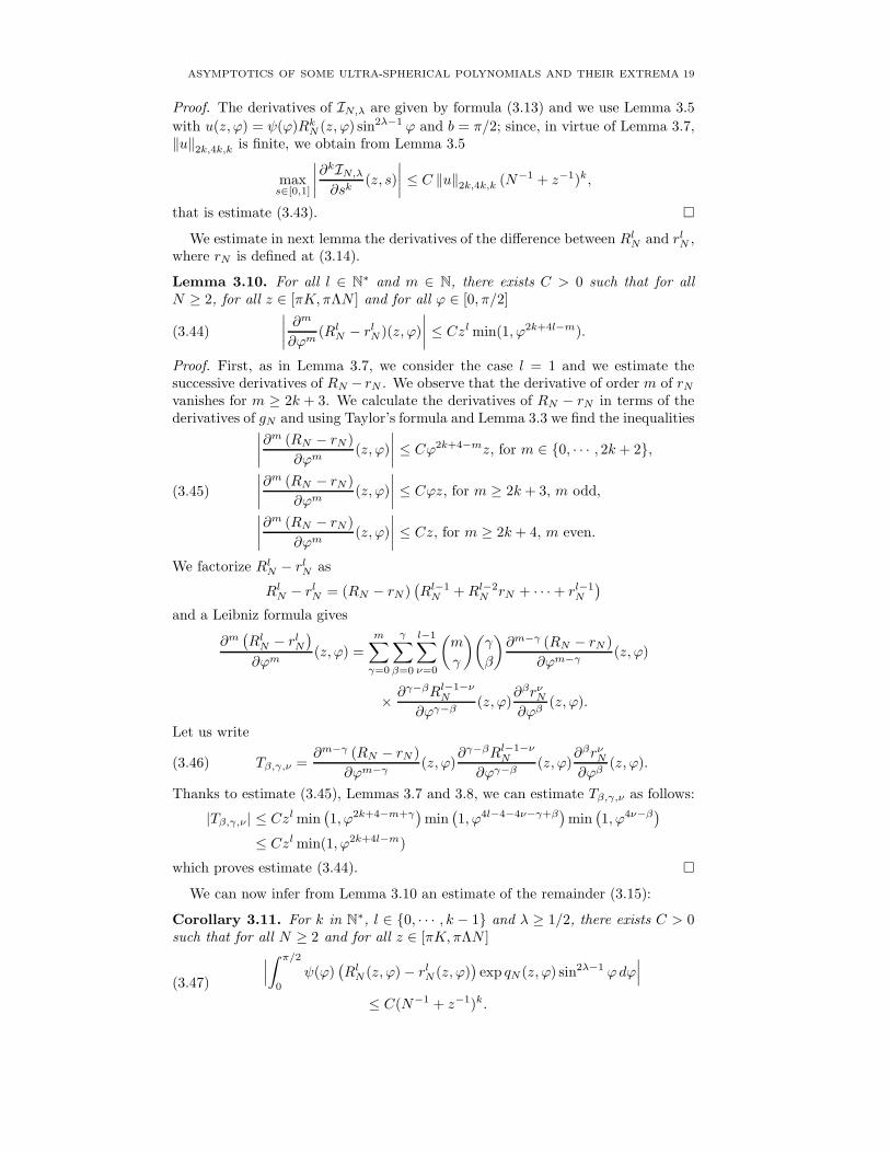
Proof. The derivatives of IN,λ are given by formula (3.13) and we use Lemma 3.5
with u(z, ϕ) = ψ(ϕ)RkN (z, ϕ) sin2λ−1 ϕ and b = π/2; since, in virtue of Lemma 3.7,
‖u‖2k,4k,k is finite, we obtain from Lemma 3.5
maxs∈[0,1]
∣
∣
∣
∣
∂kIN,λ
∂sk(z, s)
∣
∣
∣
∣
≤ C ‖u‖2k,4k,k (N−1 + z−1)k,
that is estimate (3.43). �
We estimate in next lemma the derivatives of the difference between RlN and rl
N ,where rN is defined at (3.14).
Lemma 3.10. For all l ∈ N∗ and m ∈ N, there exists C > 0 such that for allN ≥ 2, for all z ∈ [πK, πΛN ] and for all ϕ ∈ [0, π/2]
(3.44)
∣
∣
∣
∣
∂m
∂ϕm(Rl
N − rlN )(z, ϕ)
∣
∣
∣
∣
≤ Czl min(1, ϕ2k+4l−m).
Proof. First, as in Lemma 3.7, we consider the case l = 1 and we estimate thesuccessive derivatives of RN − rN . We observe that the derivative of order m of rNvanishes for m ≥ 2k + 3. We calculate the derivatives of RN − rN in terms of thederivatives of gN and using Taylor’s formula and Lemma 3.3 we find the inequalities
(3.45)
∣
∣
∣
∣
∂m (RN − rN )
∂ϕm(z, ϕ)
∣
∣
∣
∣
≤ Cϕ2k+4−mz, for m ∈ {0, · · · , 2k + 2},∣
∣
∣
∣
∂m (RN − rN )
∂ϕm(z, ϕ)
∣
∣
∣
∣
≤ Cϕz, for m ≥ 2k + 3, m odd,
∣
∣
∣
∣
∂m (RN − rN )
∂ϕm(z, ϕ)
∣
∣
∣
∣
≤ Cz, for m ≥ 2k + 4, m even.
We factorize RlN − rl
N as
RlN − rl
N = (RN − rN )(
Rl−1N +Rl−2
N rN + · · · + rl−1N
)
and a Leibniz formula gives
∂m(
RlN − rl
N
)
∂ϕm(z, ϕ) =
m∑
γ=0
γ∑
β=0
l−1∑
ν=0
(
m
γ
)(
γ
β
)
∂m−γ (RN − rN )
∂ϕm−γ(z, ϕ)
× ∂γ−βRl−1−νN
∂ϕγ−β(z, ϕ)
∂βrνN
∂ϕβ(z, ϕ).
Let us write
(3.46) Tβ,γ,ν =∂m−γ (RN − rN )
∂ϕm−γ(z, ϕ)
∂γ−βRl−1−νN
∂ϕγ−β(z, ϕ)
∂βrνN
∂ϕβ(z, ϕ).
Thanks to estimate (3.45), Lemmas 3.7 and 3.8, we can estimate Tβ,γ,ν as follows:
|Tβ,γ,ν| ≤ Czl min(
1, ϕ2k+4−m+γ)
min(
1, ϕ4l−4−4ν−γ+β)
min(
1, ϕ4ν−β)
≤ Czl min(1, ϕ2k+4l−m)
which proves estimate (3.44). �
We can now infer from Lemma 3.10 an estimate of the remainder (3.15):
Corollary 3.11. For k in N∗, l ∈ {0, · · · , k − 1} and λ ≥ 1/2, there exists C > 0
such that for all N ≥ 2 and for all z ∈ [πK, πΛN ]
∣
∣
∣
∫ π/2
0
ψ(ϕ)(
RlN (z, ϕ) − rl
N (z, ϕ))
exp qN (z, ϕ) sin2λ−1 ϕdϕ∣
∣
∣
≤ C(N−1 + z−1)k.
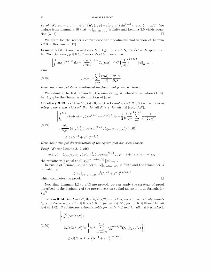
(3.47)
20 MAGALI RIBOT
Proof. We set u(z, ϕ) = ψ(ϕ)(
RlN (z, ϕ) − rl
N (z, ϕ))
sin2λ−1 ϕ and b = π/2. Wededuce from Lemma 3.10 that ‖u‖k+l,2k+4l,l is finite and Lemma 3.5 yields equa-
tion (3.47). �
We state for the reader’s convenience the one-dimensional version of Lemma7.7.3 of Hormander [12]:
Lemma 3.12. Assume a 6= 0 with Im(a) ≥ 0 and u ∈ S, the Schwartz space overR. Then for every p ∈ N∗, there exists C > 0 such that
∣
∣
∣
∣
∫
u(x)eiax2/2 dx −( a
2πi
)−1/2
Tp(u, a)
∣
∣
∣
∣
≤ C
(
1
|a|
)p+1/2
‖u‖H2p+1 ,
with
(3.48) Tp(u, a) =
p−1∑
j=0
(2ia)−j
j!
∂2ju
∂ϕ2j(0).
Here, the principal determination of the fractional power is chosen.
We estimate the last remainder; the number χN is defined at equation (1.13).Let 1[a,b] be the characteristic function of [a, b].
Corollary 3.13. Let k in N∗, l ∈ {0, · · · , k− 1} and λ such that 2λ− 1 is an eveninteger, there exists C such that for all N ≥ 2, for all z ∈ [πK, πΛN ],
∣
∣
∣
∣
∣
∫ π/2
0
ψ(ϕ)rlN (z, ϕ) sin2λ−1 ϕeχN ϕ2/2 dϕ− i
2
√
2π
χN
k+l−1∑
j=0
1
j!
1
(2χN )j
× ∂2j
∂ϕ2j
(
ψ(ϕ)rlN (z, ϕ) sin2λ−1 ϕ1[−π/2,π/2](ϕ)
)
(z, 0)
∣
∣
∣
∣
∣
≤ C(N−1 + z−1)k+1/2.
(3.49)
Here, the principal determination of the square root has been chosen.
Proof. We use Lemma 3.12 with
u(z, ϕ) = 1[−π/2,π/2](ϕ)ψ(ϕ)rlN (z, ϕ) sin2λ−1 ϕ, p = k + l and a = −iχN ,
the remainder is equal to C |χN |−(k+l+1/2) ‖u‖H2p+1 .In virtue of Lemma 3.8, the norm ‖u‖2k+2l+1,4l,l is finite and the remainder is
bounded byC ‖u‖2k+2l+1,4l,l z
l(N−1 + z−1)k+l+1/2
which completes the proof. �
Now that Lemmas 3.2 to 3.13 are proved, we can apply the strategy of proofdescribed at the beginning of the present section to find an asymptotic formula for
P(λ)N .
Theorem 3.14. Let λ = 1/2, 3/2, 5/2, 7/2, · · ·. Then, there exist real polynomialsQν,λ of degree ν for all ν ∈ N such that, for all k ∈ N∗, for all K ∈ N and for allΛ ∈ (0, 1/2), the following estimate holds for all N ≥ 2 and for all z ∈ [πK, πΛN ]:
∣
∣
∣
∣
∣
P(λ)N (cos(z/N))
− 2√πZ(λ,N)Re
{
ieizk−1∑
ν=λ−1/2
χ−(ν+1/2)N Qν,λ(χN/N)
}∣
∣
∣
∣
∣
≤ C(K,Λ, k, λ)(
N−1 + z−1)k−2λ+1
,
(3.50)

ASYMPTOTICS OF SOME ULTRA-SPHERICAL POLYNOMIALS AND THEIR EXTREMA 21
where C(K,Λ, k, λ) depends only on the displayed arguments and the constantZ(λ,N) is defined at equation (3.1).
Proof. We split (3.3) as in (3.5). Corollary 3.6 implies that the second integral ofthe right hand side of (3.5) is an O(N−1 + z−1)k.
We deduce from equation (3.12) and Corollary 3.9 that
(3.51) IN,λ(z, 1) =k−1∑
l=0
1
l!
∂lIN,λ
∂sl(z, 0) +O
(
(N−1 + z−1)k)
.
Let us obtain an expression for
∂lIN,λ
∂sl(z, 0) =
∫ π/2
0
ψ(ϕ)RlN (z, ϕ) exp qN (z, ϕ) sin2λ−1 ϕdϕ.
We replace RN by its Taylor expansion rN defined at equation (3.14). We set
JN,l,λ(z) =
∫ π/2
0
ψ(ϕ)rlN (z, ϕ) exp(χNϕ
2/2) sin2λ−1 ϕdϕ.
Corollary 3.11 implies that
∂lIN,λ
∂sl(z, 0) = eizJN,l,λ(z) +O
(
(N−1 + z−1)k)
.
We now use Corollary 3.13 to obtain an algebraic expression for JN,l,λ. Equa-tion (3.49) yields
JN,l,λ(z) = i√π
k+l−1∑
j=0
1
j!
1
(2χN )j+1/2
∂2j(rlN (z, ϕ) sin2λ−1 ϕ)
∂ϕ2j(z, 0)
+O(
(N−1 + z−1)k+1/2)
.
(3.52)
We differentiate rlN (z, ϕ) sin2λ−1 ϕ with respect to ϕ up to order 2j and we take its
value at ϕ = 0.Define
sn,λ =∂n sin2λ−1
∂ϕn(0).
We first remark that sn,λ vanishes when n is odd or n ≤ 2λ − 3. Indeed, since
2λ − 1 is even, x 7→ sin2λ−1 x is an even function and its derivatives of odd orderat ϕ = 0 vanish. Moreover, Faa di Bruno’s formula (3.17) yields
∂n sin2λ−1
∂ϕn(0) =
∑
γ∈C(n)
C(γ, n)
(
2λ− 1
l(γ)
)
l(γ)! sin2λ−1−l(γ)(0)
×l(γ)∏
j=1
sin(γjπ
2).
Consequently, when n ≤ 2λ − 3, 2λ − 1 − l(γ) is positive since l(γ) ≤ n and thus
for all γ ∈ C(n), sin2λ−1−l(γ)(0) vanishes.Therefore, for l = 0, we infer that
JN,0,λ(z) = i√π
k−1∑
j=λ−1/2
1
j!
1
(2χN )j+1/2s2j,λ +O
(
(N−1 + z−1)k+1/2)
.
Consider next the case l ≥ 1. We need first to calculate the successive even deriva-tives of rl
N (z, ϕ) at ϕ = 0. We deduce from the definition (3.14) of rN that for j in{0, · · · , 2l − 1} and for j ≥ l(k + 1) + 1, ∂2jrl
N/∂ϕ2j(z, 0) vanishes.
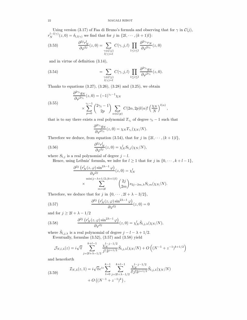
22 MAGALI RIBOT
Using version (3.17) of Faa di Bruno’s formula and observing that for γ in C(j),
rl−l(γ)N (z, 0) = δl,l(γ) we find that for j in {2l, · · · , (k + 1)l}:
∂2jrlN
∂ϕ2j(z, 0) =
∑
γ∈C(j)l(γ)=l
C(γ, j, l)∏
1≤i≤l
∂2γirN∂ϕ2γi
(z, 0)(3.53)
and in virtue of definition (3.14),
=∑
γ∈C(j)l(γ)=l
C(γ, j, l)∏
1≤i≤l
∂2γigN
∂ϕ2γi(z, 0).(3.54)
Thanks to equations (3.27), (3.26), (3.28) and (3.25), we obtain
∂2γigN
∂ϕ2γi(z, 0) = (−1)γi−1χN
×γi−1∑
p=0
(
2γi − 1
2p
)
∑
α∈C(p)
C(2α, 2p)l(α)!(χN
N
)l(α)
,
(3.55)
that is to say there exists a real polynomial Tγiof degree γi − 1 such that
∂2γigN
∂ϕ2γi(z, 0) = χNTγi
(χN/N).
Therefore we deduce, from equation (3.54), that for j in {2l, · · · , (k + 1)l},
(3.56)∂2jrl
N
∂ϕ2j(z, 0) = χl
NSl,j(χN/N),
where Sl,j is a real polynomial of degree j − l.Hence, using Leibniz’ formula, we infer for l ≥ 1 that for j in {0, · · · , k+ l− 1},
∂2j(
rlN (z, ϕ) sin2λ−1 ϕ
)
∂ϕ2j(z, 0) = χl
N
×min(j−λ+1/2,(k+1)l)
∑
m=2l
(
2j
2m
)
s2j−2m,λSl,m(χN/N).
Therefore, we deduce that for j in {0, · · · , 2l+ λ− 3/2},
(3.57)∂2j(
rlN (z, ϕ) sin2λ−1 ϕ
)
∂ϕ2j(z, 0) = 0
and for j ≥ 2l+ λ− 1/2
(3.58)∂2j(
rlN (z, ϕ) sin2λ−1 ϕ
)
∂ϕ2j(z, 0) = χl
N Sl,j,λ(χN/N),
where Sl,j,λ is a real polynomial of degree j − l − λ+ 1/2.Eventually, formulas (3.52), (3.57) and (3.58) yield
JN,l,λ(z) = i√π
k+l−1∑
j=2l+λ−1/2
χl−j−1/2N
j! 2j+1/2Sl,j,λ(χN/N) +O
(
(N−1 + z−1)k+1/2)
and henceforth
IN,λ(z, 1) = i√πeiz
k−1∑
l=0
k+l−1∑
j=2l+λ−1/2
χl−j−1/2N
l!j!2j+1/2Sl,j,λ(χN/N)
+O(
(N−1 + z−1)k)
,
(3.59)
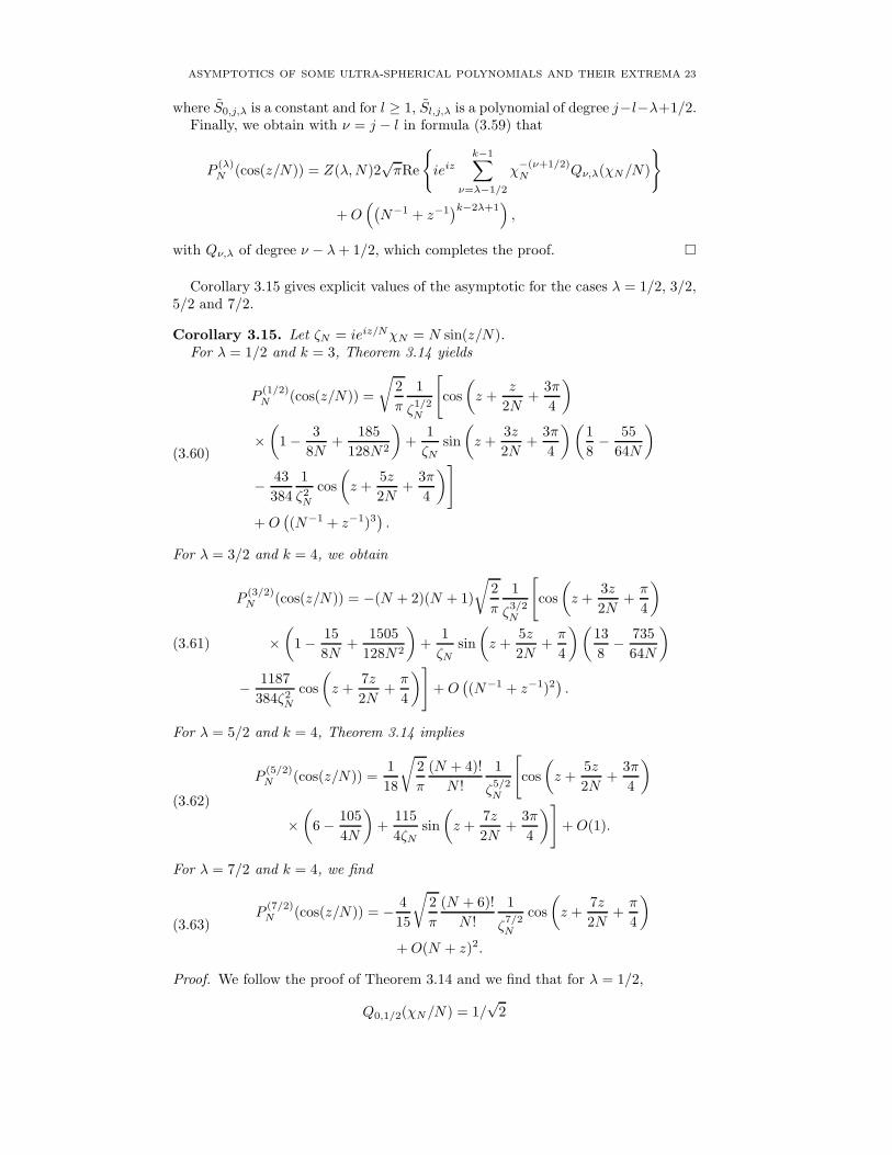
ASYMPTOTICS OF SOME ULTRA-SPHERICAL POLYNOMIALS AND THEIR EXTREMA 23
where S0,j,λ is a constant and for l ≥ 1, Sl,j,λ is a polynomial of degree j−l−λ+1/2.Finally, we obtain with ν = j − l in formula (3.59) that
P(λ)N (cos(z/N)) = Z(λ,N)2
√πRe
{
ieizk−1∑
ν=λ−1/2
χ−(ν+1/2)N Qν,λ(χN/N)
}
+O(
(
N−1 + z−1)k−2λ+1
)
,
with Qν,λ of degree ν − λ+ 1/2, which completes the proof. �
Corollary 3.15 gives explicit values of the asymptotic for the cases λ = 1/2, 3/2,5/2 and 7/2.
Corollary 3.15. Let ζN = ieiz/NχN = N sin(z/N).For λ = 1/2 and k = 3, Theorem 3.14 yields
P(1/2)N (cos(z/N)) =
√
2
π
1
ζ1/2N
[
cos
(
z +z
2N+
3π
4
)
×(
1 − 3
8N+
185
128N2
)
+1
ζNsin
(
z +3z
2N+
3π
4
)(
1
8− 55
64N
)
− 43
384
1
ζ2N
cos
(
z +5z
2N+
3π
4
)
]
+O(
(N−1 + z−1)3)
.
(3.60)
For λ = 3/2 and k = 4, we obtain
P(3/2)N (cos(z/N)) = −(N + 2)(N + 1)
√
2
π
1
ζ3/2N
[
cos
(
z +3z
2N+π
4
)
×(
1 − 15
8N+
1505
128N2
)
+1
ζNsin
(
z +5z
2N+π
4
)(
13
8− 735
64N
)
− 1187
384ζ2N
cos
(
z +7z
2N+π
4
)
]
+O(
(N−1 + z−1)2)
.
(3.61)
For λ = 5/2 and k = 4, Theorem 3.14 implies
P(5/2)N (cos(z/N)) =
1
18
√
2
π
(N + 4)!
N !
1
ζ5/2N
[
cos
(
z +5z
2N+
3π
4
)
×(
6 − 105
4N
)
+115
4ζNsin
(
z +7z
2N+
3π
4
)
]
+O(1).
(3.62)
For λ = 7/2 and k = 4, we find
P(7/2)N (cos(z/N)) = − 4
15
√
2
π
(N + 6)!
N !
1
ζ7/2N
cos
(
z +7z
2N+π
4
)
+O(N + z)2.
(3.63)
Proof. We follow the proof of Theorem 3.14 and we find that for λ = 1/2,
Q0,1/2(χN/N) = 1/√
2
24 MAGALI RIBOT
and, for ν ≥ 1,
Qν,1/2(χN/N) =∑
1≤l≤k−12l≤j≤k+l−1
j−l=ν
∑
γ1+···+γl=jγi≥2
(2j)!
j!l!
1
2j+1/2
×∏
1≤i≤l
1
(2γi)!
(
1
χN
∂2γigN
∂ϕ2γi(z, 0)
)
.
(3.64)
Let us calculate Q1,1/2 and Q2,1/2. We infer from equation (3.55) the followingderivatives of gN with respect to ϕ at ϕ = 0:
∂4gN
∂ϕ4(z, 0) = −χN
(
1 + 3χN
N
)
and
∂6gN
∂ϕ6(z, 0) = χN
(
1 + 15χN
N+ 30
χ2N
N2
)
.
We deduce from these derivatives that
Q1,1/2(χN/N) = − 1
8√
2
(
1 + 3χN
N
)
and
Q2,1/2(χN/N) =1
2√
2
(
43
192+
55χN
32N+
185χ2N
64N2
)
,
which give the asymptotic formula (3.60).We use for λ = 3/2 the successive derivatives of the square of the sine function
at ϕ = 0 which are
(3.65)∂n sin2 ϕ
∂ϕn(0) =
{
(−1)n/2+12n−1 when n is even, n ≥ 2,
0 when n is odd or n = 0.
Therefore, we obtain
Qν,3/2(χN/N) =1
2
[
(−1)ν+1
ν!2ν−1/2
+∑
1≤l≤k−12l+1≤j≤k+l−1
j−l=ν
∑
2l≤m≤j−1γ1+···+γl=m
γi≥2
(
2j
2m
)
(−1)j+m+1
22m+1/2−j
(2m)!
j!l!
×∏
1≤i≤l
1
(2γi)!
(
1
χN
∂2γigN
∂ϕ2γi(z, 0)
)
]
,
(3.66)
and more precisely, we have the following values:
Q1,3/2(χN/N) = 1/√
2,
Q2,3/2(χN/N) = − 1
2√
2
(
13
4+
15χN
4N
)
,
and
Q3,3/2(χN/N) =1
2√
2
(
1187
192+
735χN
32N+
1505χ2N
64N2
)
,
which lead to equation (3.61).
ASYMPTOTICS OF SOME ULTRA-SPHERICAL POLYNOMIALS AND THEIR EXTREMA 25
We calculate the successive derivatives of the sine function to the power 4 atϕ = 0 and we find
∂n sin4 ϕ
∂ϕn(0) =
(−1)n/2(22n−3 − 2n−1) when n is even, n ≥ 4,
0 when n is odd or
n = 0, n = 2.
These derivatives enable us to calculate:
Q2,5/2(χN/N) = 6√
2,
and
Q3,5/2(χN/N) = −√
2
(
115
4+
105
4
χN
N
)
and this yields formula (3.62).Eventually, the successive derivatives of the sine function to the power 6 at ϕ = 0
are
∂n sin6 ϕ
∂ϕn(0) =
(−1)n/2+12n−53(3n−1 − 2n+1 + 5)
when n is even, n ≥ 6,
0 when n is odd or n = 0, n = 2, n = 4.
Therefore we find thatQ3,7/2(χN/N) = 30
√2
and the calculation of formula (3.63) completes the proof. �
3.4. Asymptotics of the zeroes of the first derivatives of Legendre poly-
nomials. Now that the formulas for LN and its derivatives have been computedin Corollary 3.15, we can find an asymptotic formula for the zeroes of L′
N in theregion K ≤ k ≤ ΛN .
Theorem 3.16. Define
z0,k =π/4 + kπ
1 + 3/2N.
Then for all Λ in (0, 1/2) and for all K ∈ N, there exist C, C′ such that for allN ≥ 2 and for all integer k in {K, · · · , ⌊ΛN⌋}, there exists a unique zero zk of
P(3/2)N (cos(z/N)) in a ball of radius C′/N about z0,k and moreover the following
estimate holds
(3.67)
∣
∣
∣
∣
zk − z0,k − 13
8N tan(z0,k/N)+
22
3N2 tan(z0,k/N)
∣
∣
∣
∣
≤ C(N−1 +K−1)3.
Proof. We use the same method as in the proof of Theorem 2.1 and we use again
Lemma 2.2 to calculate an asymptotic formula for the zero zk of P(3/2)N (cos(z/N));
this function is given by formula (3.61) of Corollary 3.15.It is equivalent to calculate the zero zk of
(3.68) f(z,N) = −√
π
2
(N sin(z/N))3/2
(N + 2)(N + 1)P
(3/2)N (cos(z/N)).
We are searching this zero in the neighborhood of
z0,k =π/4 + kπ
1 + 3/2N.
We calculate f(z0,k, N) thanks to formula (3.61) of Corollary 3.15 and we obtain
(3.69) f(z0,k, N) =(−1)k
tan(z0,k/N)
(
13
8N− 509
96N2
)
+O(
(N−1 +K−1)5/2)
.
26 MAGALI RIBOT
We differentiate formula (3.68) to obtain:
∂f
∂z(z,N) =
3
2N
f(z,N)
tan(z/N)
+ 3
√
π
2
√N
(N + 2)(N + 1)sin5/2(z/N)P
(5/2)N−1 (cos(z/N))
(3.70)
and using formula (3.69) and equation (3.62) of Corollary 3.15, we find
A(k,N) =∂f
∂z(z0,k, N) = (−1)k−1 +O(N−1 +K−1).
We calculate now the second derivative of the function f using formula (3.70):
∂2f
∂z2(z,N) =
3
4N2
(
1
tan2(z/N)− 2
)
f(z,N)
+ 12
√
π
2N
N !
(N + 2)!cos(z/N) sin3/2(z/N)P
(5/2)N−1 (cos(z/N))
− 15
√
π
2N
N !
(N + 2)!sin7/2(z/N)P
(7/2)N−2 (cos(z/N)).
Let C be a positive real such that∣
∣A−1(k,N)f(z0,k, N)∣
∣ ≤ CN−1. Let z belong
to the ball of center z0,k and of radius 2CN−1. We still use formula (3.69) andequations (3.62) and (3.63) of Corollary 3.15 to compute
∂2f
∂z2(z,N) = O(N−1 +K−1).
Therefore the number M of Lemma 2.2 is finite and the number a is equal to 1. Theradius 2CN−2 has been chosen so that the hypothesis
∣
∣A−1(k,N)f(z0,k, N)∣
∣ ≤ Kis satisfied. Therefore, we have the following asymptotic formula:
zk = z0,k +13
8N tan(z0,k/N)+O
(
(N−1 +K−1)2)
.
In order to have a more precise asymptotic formula, we use once more Lemma 2.2with the same function f but in the neighborhood of
z1,k = z0,k +13
8N tan(z0,k/N).
We compute the values of f and its derivatives at z = z1,k and we find
f(z1,k, N) = (−1)k+1 22
3N2 tan(z0,k/N)+O
(
(N−1 +K−1)3)
,
∂f
∂z(z1,k, N) = (−1)k+1 +O(N−1 +K−1)
and if z belongs to the ball of center z1,k and of radius 2CN−1, the followingestimate holds:
∂2f
∂z2(z,N) = O(N−1 +K−1).
Eventually, we obtain the following asymptotic formula
zk = z0,k +13
8N tan(z0,k/N)− 22
3N2 tan(z0,k/N)+O
(
(N−1 +K−1)3)
.
�
We then have the straightforward corollary:

ASYMPTOTICS OF SOME ULTRA-SPHERICAL POLYNOMIALS AND THEIR EXTREMA 27
Corollary 3.17. Define
θ0,k =π(N − k + 1/4)
N + 1/2.
Then for all K > 0 and for all Λ ∈ (0, 1/2), there exist C, C′ such that for allN ≥ 2 and for all integer k in {K, · · · , ⌊ΛN⌋}, there exists a unique zero θk ofL′
N(cos θ) in a ball of radius C′/N2 about θ0,k; moreover the following estimateholds
(3.71)
∣
∣
∣
∣
θk − θ0,k − 13
8N2 tan θ0,k+
49
12N3 tan θ0,k
∣
∣
∣
∣
≤ C(
(N−1 +K−1)4)
.
Remark 3.18. Observe that (3.71) is compatible with (2.1), because the error termin (3.71) is large with respect to the error term in (2.1).
We end this section with the following corollary, which gives the expansion ofthe quantity σk :
Corollary 3.19. The quantities σk, K ≤ k ≤ ⌊ΛN⌋ defined at equation (1.6) havethe following expansion :
σk = 1 +2
3N2+
π2
6N2+
49
12N2 tan(η0,k)2+O
(
(N−1 +K−1)3)
.
Proof. The proof of this corollary follows the same sketch as the proof of Corol-lary 2.4. Using equation (3.71) of Corollary 3.17, we find that
LN (ξk) = (−1)N+k+1
√
2
π
1√
N sin η0,k
(
1 − 1
4N+
67
96N2− 49
24N2t2
)
+O(
(N−1 +K−1)3)
and we use equation (1.3) to compute 1/ρk:
1
ρk=
N
π sin η0,k
(
1 +1
2N+
23
24N2− 49
12N2t2
)
+O(
(N−1 +K−1)2)
.
Now, to calculate σk, we compute ξk+1 − ξk−1:
ξk+1 − ξk−1 =2 sin η0,kπ
N
(
1 − 1
2N− 11
8N2− π2
6N2
)
+O(
(N−1 +K−1)4)
and we obtain
σk =2ρk
ξk+1 − ξk−1= 1 +
2
3N2+
π2
6N2+
49
12N2t2+O
(
(N−1 +K−1)3)
.
�
References
[1] A. Averbuch, A. Cohen, and M. Israeli. A stable and accurate explicit scheme for parabolicevolution equations. http://www.ann.jussieu.fr/~cohen/para.ps.gz, 1998.
[2] Christine Bernardi and Yvon Maday. Approximations spectrales de problemes aux limiteselliptiques. Springer-Verlag, Paris, 1992.
[3] Claudio Canuto and Alfio Quarteroni. Preconditioned minimal residual methods for Cheby-shev spectral calculations. J. Comput. Phys., 60(2):315–337, 1985.
[4] Claudio Canuto. Stabilization of spectral methods by finite element bubble functions. Com-put. Methods Appl. Mech. Engrg., 116(1-4):13–26, 1994. ICOSAHOM’92 (Montpellier, 1992).
[5] Mark H. Carpenter, David Gottlieb, and Chi-Wang Shu. On the conservation and convergenceto weak solutions of global schemes. J. Sci. Comput., 18(1):111–132, 2003.
[6] Piero de Mottoni and Michelle Schatzman. The Thual-Fauve pulse: Skew stabilization. Tech-
nical Report 304, Equipe d’Analyse Numerique de Lyon, 1999. http://numerix.univ-lyon1.fr/publis/publiv/1999/schatz1609/publi.ps.gz.

28 MAGALI RIBOT
[7] M. Deville and E. Mund. Chebyshev pseudospectral solution of second-order elliptic equationswith finite element preconditioning. J. Comput. Phys., 60(3):517–533, 1985.
[8] M. O. Deville and E. H. Mund. Finite-element preconditioning for pseudospectral solutionsof elliptic problems. SIAM J. Sci. Statist. Comput., 11(2):311–342, 1990.
[9] Luigi Gatteschi. Uniform approximation of Christoffel numbers for Jacobi weight. In Nu-merical integration, III (Oberwolfach, 1987), volume 85 of Internat. Schriftenreihe Numer.Math., pages 49–59. Birkhauser, Basel, 1988.
[10] E. Hairer, S. P. Nørsett, and G. Wanner. Solving ordinary differential equations. I, volume 8of Springer Series in Computational Mathematics. Springer-Verlag, Berlin, second edition,1993. Nonstiff problems.
[11] P. Haldenwang, G. Labrosse, S. Abboudi, and M. Deville. Chebyshev 3-D spectral and 2-Dpseudospectral solvers for the Helmholtz equation. J. Comput. Phys., 55(1):115–128, 1984.
[12] Lars Hormander. The analysis of linear partial differential operators. I. Springer Study Edi-tion. Springer-Verlag, Berlin, second edition, 1990. Distribution theory and Fourier analysis.
[13] Steven A. Orszag. Spectral methods for problems in complex geometries. J. Comput. Phys.,37(1):70–92, 1980.
[14] Seymour V. Parter. On the Legendre-Gauss-Lobatto points and weights. J. Sci. Comput.,14(4):347–355, 1999.
[15] Seymour V. Parter. Preconditioning Legendre special collocation methods for elliptic prob-lems. I. Finite difference operators. SIAM J. Numer. Anal., 39(1):330–347 (electronic), 2001.
[16] Seymour V. Parter. Preconditioning Legendre spectral collocation methods for elliptic prob-lems. II. Finite element operators. SIAM J. Numer. Anal., 39(1):348–362 (electronic), 2001.
[17] Seymour V. Parter and Ernest E. Rothman. Preconditioning Legendre spectral collocationapproximations to elliptic problems. SIAM J. Numer. Anal., 32(2):333–385, 1995.
[18] Alfio Quarteroni and Elena Zampieri. Finite element preconditioning for Legendre spec-tral collocation approximations to elliptic equations and systems. SIAM J. Numer. Anal.,29(4):917–936, 1992.
[19] Magali Ribot. Etude theorique de methodes numeriques pour les systemes de reaction-diffusion; application a des equations paraboliques non lineaires et non locales. PhD thesis,Universite Claude Bernard – Lyon 1, December 2003. http://math.unice.fr/~ribot/these.pdf.
[20] Gabor Szego. Orthogonal polynomials. American Mathematical Society, Providence, R.I.,fourth edition, 1975. American Mathematical Society, Colloquium Publications, Vol. XXIII.
Laboratoire Dieudonne, Universite de Nice-Sophia Antipolis, 06108 Nice Cedex 2,France. Fax : (+33) 4 93 51 79 74
E-mail address: [email protected]


![Asymptotic analysis of the Askey-scheme I: from Krawtchouk ...dominicd/charl15.pdf · The generalized Charlier polynomials were analyzed in [14], [17], [33], [34] and [40]. Asymptotics](https://img.pdfslide.net/doc/110x75/60f83acbf76c897c682d3032/asymptotic-analysis-of-the-askey-scheme-i-from-krawtchouk-dominicdcharl15pdf.jpg)
![RELATIVE ASYMPTOTICS FOR ORTHOGONAL MATRIX … · arXiv:1003.0852v1 [math.CA] 3 Mar 2010 RELATIVE ASYMPTOTICS FOR ORTHOGONAL MATRIX POLYNOMIALS A. BRANQUINHO, F. MARCELLAN, AND A](https://img.pdfslide.net/doc/110x75/5ecb980806364b24ec1cdc37/relative-asymptotics-for-orthogonal-matrix-arxiv10030852v1-mathca-3-mar-2010.jpg)


![arXiv:0905.1684v2 [math-ph] 18 Sep 2009The strong asymptotics of polynomials orthogonal with respect to exponential weights (i.e., Hermite polynomials, Freud weights, etc.) has received](https://img.pdfslide.net/doc/110x75/5f7026728d0e116a257fdc9f/arxiv09051684v2-math-ph-18-sep-2009-the-strong-asymptotics-of-polynomials-orthogonal.jpg)