arX

iv:1

307.

2566

v2 [

astr

o-ph

.CO

] 9

Dec

201

3Draft version December 10, 2013Preprint typeset using LATEX style emulateapj v. 5/2/11

THE EFFECT OF WEAK LENSING ON DISTANCE ESTIMATES FROM SUPERNOVAE

Mathew Smith*,1,2, David J. Bacon3, Robert C. Nichol3, Heather Campbell3, Chris Clarkson4, Roy Maartens1,3,Chris B. D’Andrea3, Bruce A. Bassett2,5, David Cinabro6, David A. Finley7, Joshua A. Frieman7,8,9, Lluis

Galbany10,11, Peter M. Garnavich12, Matthew D. Olmstead13, Donald P. Schneider14,15 Charles Shapiro16 &Jesper Sollerman17

Draft version December 10, 2013

ABSTRACT

Using a sample of 608 Type Ia supernovae from the SDSS-II and BOSS surveys, combined witha sample of foreground galaxies from SDSS-II, we estimate the weak lensing convergence for eachsupernova line-of-sight. We find that the correlation between this measurement and the Hubbleresiduals is consistent with the prediction from lensing (at a significance of 1.7σ). Strong correlationsare also found between the residuals and supernova nuisance parameters after a linear correction isapplied. When these other correlations are taken into account, the lensing signal is detected at 1.4σ.We show for the first time that distance estimates from supernovae can be improved when lensingis incorporated by including a new parameter in the SALT2 methodology for determining distancemoduli. The recovered value of the new parameter is consistent with the lensing prediction. UsingCMB data from WMAP7, H0 data from HST and SDSS BAO measurements, we find the best-fitvalue of the new lensing parameter and show that the central values and uncertainties on Ωm and ware unaffected. The lensing of supernovae, while only seen at marginal significance in this low redshiftsample, will be of vital importance for the next generation of surveys, such as DES and LSST, whichwill be systematics dominated.

Subject headings: cosmology: observations — distance scale – supernovae: general — surveys

1. INTRODUCTION

Type Ia supernovae (SNe Ia) are currently the bestcosmological “standard candles” and can be observedto high redshift. Extensive searches for SNe Ia have

* matsmith2@gmail.com1 Department of Physics, University of the Western Cape,

Cape Town, 7535, South Africa2 South African Astronomical Observatory, P.O. Box 9, Ob-

servatory 7935, SA3 Institute of Cosmology and Gravitation, University of

Portsmouth, Portsmouth, PO1 3FX, UK4 Astrophysics, Cosmology and Gravity Centre (ACGC), De-

partment of Mathematics and Applied Mathematics, Universityof Cape Town, Rondebosch, 7701, SA

5 African Institute for Mathematical Sciences, 6-8 MelroseRoad, Muizenberg 7945, SA

6 Wayne State University, Department of Physics and Astron-omy, Detroit, MI 48202, USA

7 Center for Particle Astrophysics, Fermi National AcceleratorLaboratory, P.O. Box 500, Batavia, IL 60510, USA

8 Kavli Institute for Cosmological Physics, The University ofChicago, 5640 South Ellis Avenue, Chicago, IL 60637, USA

9 Department of Astronomy and Astrophysics, The Universityof Chicago, 5640 South Ellis Avenue, Chicago, IL 60637, USA

10 CENTRA Centro Multidisciplinar de Astrofısica, InstitutoSuperior Tecnico, Av. Rovisco Pais 1, 1049-001 Lisbon, Portu-gal

11 Institut de Fısica d’Altes Energies, Universitat Autonomade Barcelona, E-08193 Bellaterra (Barcelona), Spain

12 Department of Physics, University of Notre Dame, NotreDame, IN 46556

13 Department of Physics and Astronomy, University of Utah,Salt Lake City, UT 84112

14 Department of Astronomy and Astrophysics, The Pennsyl-vania State University, University Park, PA 16802

15 Institute for Gravitation and the Cosmos, The Pennsylva-nia State University, University Park, PA 16802

16 NASA Jet Propulsion Laboratory; California Institute ofTechnology

17 The Oskar Klein Centre, Department of Astronomy, Al-baNova, SE-106 91 Stockholm, Sweden

been carried out over the last decade to map the expan-sion history of the Universe with cosmic time. Observa-tions of SNe Ia have produced convincing evidence thatthe Universe has undergone a recent period of acceler-ated expansion (Riess et al. 1998; Perlmutter et al. 1999;Astier et al. 2006; Kessler et al. 2009; Lampeitl et al.2010a; Sullivan et al. 2011) leading to the inference thatthe energy density of the Universe is dominated by “darkenergy”. By combining measurements of SNe Ia dis-tances, over a wide range of redshift, with other cos-mological probes such as measurements of the CosmicMicrowave Background (CMB) and Baryon Acoustic Os-cillations (BAO), the equation of state of dark energy isknown to an accuracy of 7% (Sullivan et al. 2011) and isconsistent with a cosmological constant.While SNe Ia have been calibrated as “standard can-

dles”, their luminosities retain a significant scatter aboutthe best-fitting cosmological model, indicating that theyare influenced by additional effects such as extinction(circumstellar and/or host galaxy dust), differences inthe SN Ia progenitor, photometric calibration and possi-bly gravitational lensing. These systematic uncertain-ties can increase the dispersion of the SN Ia popula-tion’s luminosity, and reduce the precision of the in-ferred constraints on cosmological parameters. Recentresults from the Planck satellite (Planck Collaboration2013) show some tension between the value of Ωm de-termined by Planck and the most recent SN Ia datasets,suggesting that there could be residual systematic errorsin either the SNe data, the Planck data or both thatare not properly accounted for. Understanding and cor-recting for systematic uncertainties will be important inorder to deliver the expected improvement in dark en-ergy constraints from forthcoming surveys, such as the

2 Smith et al.

Dark Energy Survey (Bernstein et al. 2012) and LSST(LSST Science Collaboration 2009), which will observethousands of SNe to high redshift.Recent progress in improving the standardization of

SNe Ia has focussed on correlations between host galaxyproperties and the observed SN parameters (Kelly et al.2010; Lampeitl et al. 2010b; Sullivan et al. 2010). Astrong correlation has been observed between the abso-lute magnitude of SNe Ia and the total stellar mass of thehost galaxy. Applying this observed correlation does helpreduce the scatter on the Hubble diagram, thus improv-ing the cosmological parameter estimates (Sullivan et al.2011). However, the origin of this empirical correction re-mains unclear (D’Andrea et al. 2011; Gupta et al. 2011;Galbany et al. 2012; Hayden et al. 2013) and may evolvewith redshift.One expected and well-understood cause for an

increase in the dispersion of SN Ia magnitudes isthe weak gravitational lensing of SN light by theintervening matter along the line of sight (Frieman1996; Holz 1998; Kantowski 1998; Metcalf 1999; Wang1999; Bergstrom et al. 2000; Amanullah et al. 2003;Menard et al. 2003; Holz and Linder 2005; Cooray et al.2006; Amendola et al. 2010; Clarkson et al. 2012;Marra et al. 2013; Fleury et al. 2013). Correlationsbetween the background SNe (point sources) and theforeground clustered mass will cause SNe Ia to appearbrighter, relative to the mean of the SN Ia population,when the lensing convergence along the line of sight ispositive, and conversely de-magnified when it is negative.(Note that there is an additional Doppler contributionto the convergence which acts in the opposite sense andcan be significant at low redshifts (Bolejko et al. 2013).)This effect will not significantly bias the cosmologicalparameters (Sarkar et al. 2008; Jonsson et al. 2008),but if uncorrected, will cause additional scatter in theobserved SN Ia magnitudes leading to an increase intheir distance uncertainty. This additional dispersion isgreater at high redshifts due to the additional extentof the light-path. Wang (2000) used simulated datawith weak lensing noise to show that the estimatedcosmological parameters will be unbiased if the fittingis carried out in flux space, suggesting a flux-averagingapproach as lensing conserves total flux.Several studies have addressed the expected increased

dispersion in SN Ia magnitudes due to weak gravita-tional lensing. Wambsganss et al. (1997) considered ray–tracing in cosmological simulations and found an in-creased scatter of 0.02 mag for SNe Ia at z = 0.5, whileMenard et al. (2003) and Takada and Hamana (2003)showed that lensing causes variations of δm . 0.01.These effects are presently sub-dominant to the cur-rent SN Ia magnitude uncertainties of δm ≃ 0.15 mag.Frieman (1996) shows that for sources at z = 1, den-sity fluctuations could increase the observed dispersionby 30%. Gunnarsson et al. (2006) showed that for anSN Ia at z = 1.5, the dispersion due to lensing is com-parable to the intrinsic SN Ia scatter, and introduced amethod to reduce the scatter from 7% to 3%.The effect of lensing on high redshift SN Ia datasets

has been studied by several authors. Williams and Song(2004) used a sample of 55 SNe Ia with z ≥ 0.35 fromthe Supernova Cosmology Project and High-z Super-nova Search datasets (Tonry et al. 2003) and correlated

their brightness with foreground galaxies from the APMNorthern Sky Catalogue (Irwin et al. 1994). They de-tected a correlation consistent with lensing at the > 99%confidence level, but the observed difference of 0.3 mag,between the most magnified and de–magnified SNe Ia, isfar larger than expected. Menard and Dalal (2005) used44 SNe Ia from the Riess et al. (2004) dataset in combi-nation with galaxies from the photometric catalogue ofthe Sloan Digital Sky Survey (SDSS) and found no de-tectable correlation on scales of one to ten arcminutes.Wang (2005) convolved the intrinsic distribution of SNeIa, using the Riess et al. (2004) sample, with magnifica-tion distributions of point sources, finding marginal evi-dence for a non-Gaussian tail at high redshift, and a shiftin the peak brightness towards the faint end, both indi-cators of weak lensing. Mortsell et al. (2001) consideredSN 1997ff at z = 1.77 and showed that careful mod-eling of foreground galaxies is required to estimate thelensing signal, finding a large range of possible magnifi-cations. Jonsson et al. (2007) found a signal consistentwith lensing at ∼ 90% confidence level using 26 SNe inthe GOODS field and an aperture of one arcminute toestimate the foreground galaxy density.Recently, several authors have looked for lensing using

the larger, more homogeneous, three-year data releaseof the Supernova Legacy Survey (SNLS) (Astier et al.2006). Kronborg et al. (2010) combined this datasetwith a deep photometric catalogue of foreground galax-ies (with inferred masses) to find evidence for a lensingsignal at 2.3σ, while Jonsson et al. (2010) detected a sig-nal at 92% confidence, simultaneously constraining theproperties of the galaxy dark matter haloes. However,Karpenka et al. (2013) obtained only a marginal detec-tion of a lensing signal when using a Bayesian analysisof the same dataset, and only found weak constraints onthe dark matter halo parameters.The expected lensing contribution to the scatter of SN

Ia magnitudes is not anticipated to be strong for currentSN Ia samples, due to the small number of confirmed SNeIa, the limited redshift range surveyed and photomet-ric uncertainties. However, with future surveys, such asDES and LSST producing thousands of SNe Ia to z > 1,the gravitational lensing effect should become important,especially to achieve the required high precision on thecosmological parameters. It is therefore important to de-velop a model-independent formalism to characterize andaccount for this effect.In this paper, we develop a scheme to measure and

correct for the effect of weak gravitational lensing onType Ia supernova distances. Using a new sample of608 SNe Ia obtained from the SDSS-II SNe Survey, with0.2 < z < 0.6, supplemented by spectroscopic hostgalaxy redshifts observed as part of the BOSS survey(Eisenstein et al. 2011; Dawson et al. 2013), we correlatethis SN sample with foreground galaxies from SDSS-II toconstrain the possible lensing signal. We also extend pre-vious analyses by simultaneously constraining the lens-ing signal alongside other SN nuisance parameters, thusimproving the standardization of SNe Ia.The outline of this paper is as follows. In §2 we de-

scribe the SN Ia and galaxy data used in this analysis.§3 describes the analysis used to estimate the lensing sig-nal, while in §4, we present the measured correlation, andits impact on the cosmological parameters. In §4.4, we

Weak Lensing of SNe Ia 3

discuss how the lensing signal will affect the inferred dis-tances to SNe Ia and constrain the bias of our foregroundgalaxy sample. Finally, we conclude in §5.

2. DATA

2.1. The SDSS-II Supernova Survey

From 2005 to 2007, the SDSS-II SN Survey(Frieman et al. 2008; Sako et al. 2008) carried out a ded-icated search for intermediate-redshift SNe Ia from re-peated scans of the equatorial “Stripe82” region cov-ering a total of 300 deg2. The SDSS 2.5m Telescope(Gunn et al. 1998) carried out multi-colour ugriz imag-ing for three months a year (September to November)with an average cadence of 3 days. Using a suite of in-ternational telescopes (Zheng et al. 2008; Ostman et al.2011; Konishi et al. 2011b), over 500 SNe Ia were spec-troscopically confirmed, with several thousand additionalprobable SNe Ia identified through their high qualitylight-curves.This sample of SDSS-II SNe Ia has now been

used to constrain cosmological parameters (Kessler et al.2009; Lampeitl et al. 2010a; Sollerman et al. 2009),measure the SN Ia rate (Dilday et al. 2008, 2010;Smith et al. 2012), examine the rise-time distribution(Hayden et al. 2010) and study the correlation betweenSNe Ia and their host galaxies (Lampeitl et al. 2010b;D’Andrea et al. 2011; Gupta et al. 2011; Galbany et al.2012; Hayden et al. 2013) and spectroscopic indicators(Nordin et al. 2011a,b; Konishi et al. 2011a; Foley et al.2012).

2.2. BOSS Ancillary Program

In 2009, an ancillary program was initiated as partof the SDSS-III Baryon Oscillation Spectroscopic Sur-vey (BOSS) (Olmstead et al. 2013; Dawson et al. 2013)to obtain the spectra and redshifts of the host galaxies ofa large sample of supernova candidates detected by theSDSS-II SN Survey. This program was designed to un-derstand possible incompletenesses and biases in the orig-inal real-time spectroscopic follow-up. In total, spectrawere obtained for 3761 host galaxies, producing 3520 con-firmed redshifts of SN candidates (and other transients)to a limiting galaxy magnitude of r < 22.0. Full detailsof the target selection and data reduction for this sampleof galaxies can be found in Campbell et al. (2013), whiledetails of the data analysis and redshifts for the sampleare presented in Olmstead et al. (2013).The details of how a robust cosmological Hubble di-

agram is constructed using these host galaxy redshiftsin conjunction with the original SDSS-II SN light curvedata is presented in Campbell et al. (2013). Using a com-bination of the PSNID (Sako et al. 2011) and SALT2(Guy et al. 2007) techniques, combined with stringentdata-quality cuts, a new and robust sample of 752 pho-tometrically classified SNe Ia covering a redshift range0.05 < z < 0.55 was constructed from the BOSS andSDSS-II galaxy samples. Using realistic simulations,Campbell et al. (2013) showed that this sample is over70% efficient in detecting SNe Ia over this redshift range,with only 4% probable contamination from non-Ia su-pernovae. Campbell et al. (2013) further demonstratedthat this sample provides competitive cosmological con-straints, compared to the spectroscopically confirmed

samples from SNLS.For this work, the distance modulus to an SN Ia is

determined using the SALT2 light-curve fitting method(Guy et al. 2007) and is defined as

µ = mB −M + αx1 − βc+ µcorr(z), (1)

where mB = 10.635 − 2.5 logx0. x0, x1 and c are SNeparameters determined through fitting of the individ-ual light-curves, and correspond to the peak magnitude,stretch and color of each SN. HereM is the absolute peakmagnitude of a standard SNe Ia (assumed to be −19.0for this analysis) and α and β are global SALT2 param-eters that describe the relationship between the stretchand colour of an SN Ia and the absolute brightness. Wealso include a correction for Malmquist bias (µcorr(z))which is discussed, and calculated for this sample, inCampbell et al. (2013).For our fiducial analysis, we use α = 0.22, β = 3.12 and

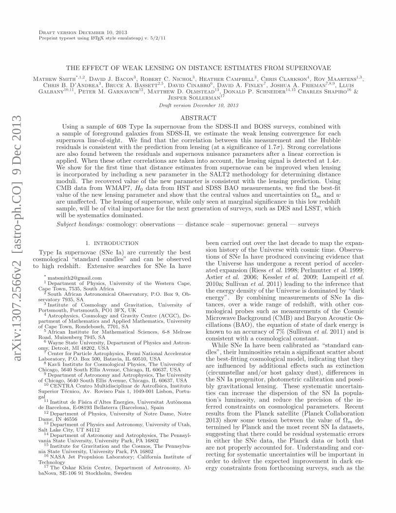
the best-fitting cosmology taken from Campbell et al.(2013) of (Ωm,ΩΛ,Ωk, w) = (0.27, 0.73, 0.0,−0.95) andH0 = 73.8kms−1 Mpc−1 from the SH0ES survey(Riess et al. 2011). As with other SN analyses, wealso include an intrinsic dispersion for the sample ofσint = 0.12 mag, which provides a reduced χ2 close tounity for the best fit. To remove possible bias from largeoutliers, which can significantly impact any correlation,a 5σ clip on residuals from the Hubble diagram using thebest-fitting cosmological parameters, has been applied tothe data, removing three SNe Ia in total, reducing oursample to 749 SNe Ia.Figure 1 gives the Hubble diagram for the 749 photo-

metrically classified SNe Ia taken from Campbell et al.(2013) and Figure 2 shows the redshift histogram forthese SNe Ia. Our fiducial sample consists of 608 SNeIa with 0.2 < z < 0.6. This selection is discussed in §3.This is one of the largest SNe Ia datasets in existence andis appropriate for the lensing study discussed in this pa-per because of the uniform selection, consistent relativephotometric calibration (all of the SNe Ia data is from asingle survey) and high completeness. The sample alsopushes to higher redshift than the spectroscopically con-firmed SNe sample of SDSS-II, which helps in our searchfor a gravitational lensing signal.

2.3. Spectroscopic Galaxy Catalogue

In addition to background SNe, we need tracers ofthe foreground mass density in order to obtain a lensingcorrelation between SN brightness and foreground den-sity. Ideally, these foreground tracers would have accu-rate spectroscopic redshifts allowing us to unambiguouslydetermine their location relative to the SNe. This also fa-cilitates a better prediction of the expected lensing signaltaking into account the relative distances between us, theSNe and foreground lenses. Fortunately the “Stripe82”region of the SDSS has a significantly higher density ofspectroscopic data compared to the average for SDSS dueto a number of other ancillary programs as outlined in theData Release 8 (DR8) of the SDSS (Aihara et al. 2011).In total, there are over 800,000 spectroscopic galaxy red-shifts in DR8 in the “Stripe82” region.We have not used all these galaxy redshifts, but in-

stead use only the ancillary programs with well-definedselection criteria that span the whole area of “Stripe82”.

4 Smith et al.

Fig. 1.— Upper: Hubble diagram for the 749 SNe used in this analysis. Lower: Residuals from the above Hubble diagram, consideringthe best-fitting cosmology from Campbell et al. (2013). The redshift cut of z > 0.2, used to define the fiducial sample, is also shown.

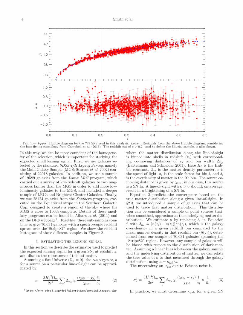
In this way, we can be more confident of the homogene-ity of the selection, which is important for studying theexpected small lensing signal. First, we use galaxies se-lected by the standard SDSS-I/II Legacy Survey, namelythe Main Galaxy Sample (MGS; Strauss et al. 2002) con-sisting of 22918 galaxies. In addition, we use a sampleof 19589 galaxies from the Low-z LRG program, whichcarried out a survey of low-redshift galaxies to two mag-nitudes fainter than the MGS in order to add more low-luminosity galaxies to the MGS, and included a deepersample of LRGs and Brightest Cluster Galaxies. Finally,we use 28124 galaxies from the Southern program, exe-cuted on the Equatorial stripe in the Southern GalacticCap, designed to create a region of the sky where theMGS is close to 100% complete. Details of these ancil-lary programs can be found in Aihara et al. (2011) andon the DR8 webpage1. Together, these sub-samples com-bine to give 70,631 galaxies with a spectroscopic redshiftspread over the“Stripe82” region. We show the redshifthistogram of these different samples in Figure 2.

3. ESTIMATING THE LENSING SIGNAL

In this section we describe the estimator used to predictthe expected lensing signal for a given SN, at redshift z,and discuss the robustness of this estimator.Assuming a flat Universe (Ωk = 0), the convergence, κ

for a source on a particular line-of-sight can be approxi-mated by,

κ =3H0

2Ωm

2c2

∑

i

∆χiχi

(χSN − χi)

χSN

δiai, (2)

1 http://www.sdss3.org/dr8/algorithms/special target.php

where the matter distribution along the line-of-sightis binned into shells in redshift (zi) with correspond-ing co-moving distances of χi and bin width ∆χi

(Bartelmann and Schneider 2001). Here H0 is the Hub-ble constant, Ωm is the matter density parameter, c isthe speed of light, ai is the scale factor for bin i, and δiis the overdensity of matter in the ith bin. The source co-moving distance is given by χSN; in our case, this sourceis a SN Ia. A line-of-sight with κ > 0 should, on average,result in a brightening of a SN Ia.Equation 2 predicts the convergence based on the

true matter distribution along a given line-of-sight. In§2.3, we introduced a sample of galaxies that can beused to trace that matter distribution. This distribu-tion can be considered a sample of point sources that,when smoothed, approximates the underlying matter dis-tribution. We estimate κ by replacing δi in Equation2 with δni

= [n(zi)− n(zi)]/n(zi), which is the galaxyover-density in a given redshift bin compared to themean number density in that redshift bin (n(zi)), deter-mined from our sample of 70,631 galaxies spanning the“Stripe82” region. However, any sample of galaxies willbe biased with respect to the distribution of dark mat-ter. Assuming a linear bias b between the galaxy sampleand the underlying distribution of matter, we can relatethe true value of κ to that measured through the galaxydistribution, using κ = κgal/b.The uncertainty on κgal due to Poisson noise is

σ2κ =

3H02Ωm

2c2

∑

i

∆χiχi

(χSN − χi)

χSN

1

ai×

1

ni

. (3)

In practice, we must determine κgal, for a given SN

Weak Lensing of SNe Ia 5

Fig. 2.— Normalized redshift distribution for the 749 SNe Ia (red) and 70631 galaxies used in this analysis, as described in §2. Theredshift histograms for the three galaxy sub-samples are shown cumulatively.

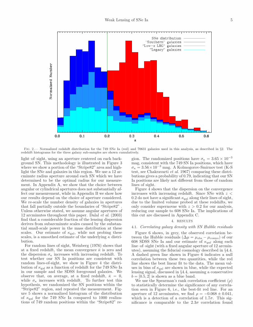
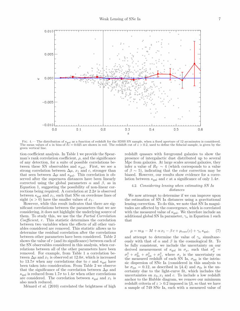
light–of–sight, using an aperture centered on each back-ground SN. This methodology is illustrated in Figure 3where we show a portion of the “Stripe82” area and high-light the SNe and galaxies in this region. We use a 12 ar-cminute radius aperture around each SN which we havedetermined to be the optimal radius for our measure-ment. In Appendix A, we show that the choice betweenangular or cylindrical apertures does not substantially af-fect our measurement, while in Appendix B we show howour results depend on the choice of aperture considered.We re-scale the number density of galaxies in aperturesthat fall partially outside the boundaries of “Stripe82” .Unless otherwise stated, we assume angular apertures of12 arcminutes throughout this paper. Dalal et al. (2003)find that a considerable fraction of the lensing dispersionderives from subarcminute scales caused by the substan-tial small-scale power in the mass distribution at thesescales. Our estimate of κgal, while not probing thesescales, is a smoothed estimate of the underlying κ distri-bution.For random lines of sight, Weinberg (1976) shows that

at a fixed redshift, the mean convergence κ is zero andthe dispersion σκ increases with increasing redshift. Totest whether our SN Ia positions are consistent withrandom lines-of-sight, we show in Figure 4 the distri-bution of κgal as a function of redshift for the 749 SNe Iain our sample and the SDSS foreground galaxies. Weobserve that, on average, at a fixed redshift, κ = 0,while σκ increases with redshift. To further test thishypothesis, we randomized the SN positions within the“Stripe82” region, and repeated the measurement. Fig-ure 5 shows a normalized histogram of the distributionof κgal for the 749 SNe Ia compared to 1000 realiza-tions of 749 random positions within the “Stripe82” re-

gion. The randomized positions have σκ = 3.65 × 10−3

mag, consistent with the 749 SN Ia positions, which haveσκ = 3.56×10−3 mag. A Kolmogorov-Smirnov test (K-Stest, see Chakravarti et al. 1967) comparing these distri-butions gives a probability of 0.79, indicating that our SNIa positions are likely not different from those of randomlines of sight.Figure 4 shows that the dispersion on the convergence

increases with increasing redshift. Since SNe with z <0.2 do not have a significant κgal along their lines of sight,due to the limited volume probed at these redshifts, weonly consider supernovae with z > 0.2 for our analysis,reducing our sample to 608 SNe Ia. The implications ofthis cut are discussed in Appendix C.

4. RESULTS

4.1. Correlating galaxy density with SN Hubble residuals

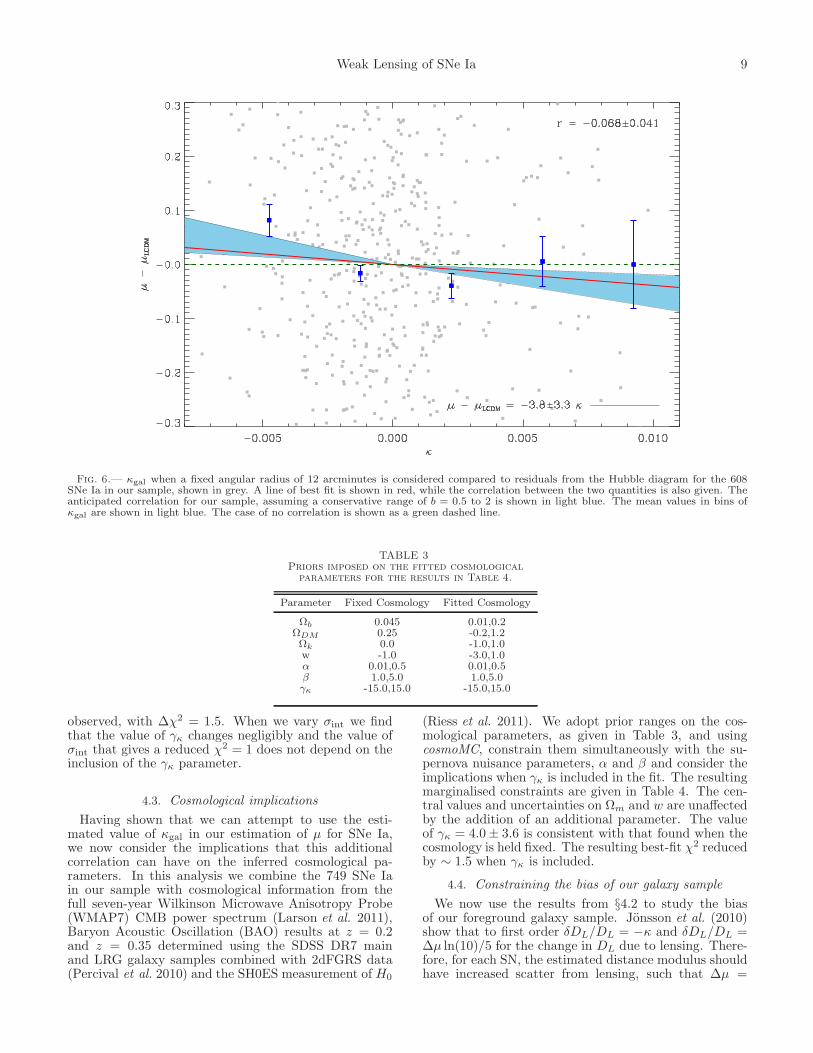
Figure 6 shows, in grey, the observed correlation be-tween the Hubble residuals (∆µ = µobs − µcosmo) of our608 SDSS SNe Ia and our estimate of κgal along eachline–of–sight (with a fixed angular aperture of 12 arcmin-utes), assuming the fiducial cosmology described in §4.4.A dashed green line shown in Figure 6 indicates a nullcorrelation between these two quantities, while the redline shows the best linear fit to the data. The mean val-ues in bins of κgal are shown in blue, while the expectedlensing signal, discussed in §4.4, assuming a conservativeb = [0.5, 2] is shown as a blue band.We use the Spearman’s rank correlation coefficient (ρ)

to statistically determine the significance of any correla-tion seen in Figure 6, i.e., the best-fit red line. For anaperture of 12 arcminutes, we find ρ = −0.068 ± 0.041,which is a detection of a correlation of 1.7σ. This sig-nificance is comparable to the 2.3σ correlation found

6 Smith et al.

Fig. 3.— An illustration of the methodology used to search for SN lensing in our SDSS SN sample. We only show a small portion of the“Stripe82” field and highlight with stars the SDSS SNe. Around each SN, we show the projected 12 arcminute aperture used to calculateκgal in cyan. We show galaxies within an aperture and in the foreground of a SN as blue dots. Galaxies within an aperture, but behindthe SNe are shown in black.

by Kronborg et al. (2010) using 233 SNe Ia from theSNLS dataset and Jonsson et al. (2007) using 26 SNeIa from the GOODS field who found a tentative de-tection of lensing at 90% confidence level. This lim-ited significance correlation is consistent with the ex-pected weak lensing signal for our data. SNe Ia withκgal > 0 have ∆µ = −0.024 ± 0.017 mag, compared to∆µ = 0.010± 0.014 mag for those with κgal < 0.

4.1.1. Comparing to the expected lensing signal

To determine if the scatter we observe on κgal in Fig-ures 4 and 6 is consistent with expectation, we estimatethe theoretical error on κ, by considering κ averaged inan angular aperture of radius θ. Following the analy-sis of Bartelmann and Schneider (2001), we calculate theweight function, W (χ), defined as,

W (r) =

∫ χH

χ

dχ′G(χ′)fκ(χ

′ − χ)

fκ(χ′), (4)

where χ is the comoving distance, and G(χ)dχ =pz(z)dz. Assuming a flat Universe such that fk(χ) = χ,we calculate Pκ, by integrating W and the power spec-trum (Pδ),

Pκ(l) =9H4

0Ω20

4c2

∫ wH

0

dχW 2(χ)

a2(χ)Pδ

(

l

fK(χ), χ

)

, (5)

where a is the scale factor. The rms scatter on κ, withina circular aperture of radius θ is,

〈κ2av(θ)〉 = 2π

∫

∞

0

ldlPκ(l)

[

J1(lθ)

πlθ

]2

, (6)

where J1(x) is the first order Bessel function of the firstkind. Considering an aperture of 12’, with (Ωm,ΩΛ, w) =(0.3, 0.7,−1.0), σ8 = 0.8 and H0 = 70 kms−1 Mpc−1

we use the package iCosmo (Refregier et al. 2011) tocalculate the non-linear power spectrum using the fit-ting formula of Peacock and Dodds (1994) and determine〈κ2

av(θ)〉 from Equations 4, 5 and 6. We find an expectedrms scatter on κ of 0.44% over the redshift range for thissupernova sample, consistent with the value of 0.36% forour dataset as seen in Figures 4, 5 and 6.

4.1.2. Determining the source and significance of thecorrelation

The mild correlation seen in Figure 6 could be due toa systematic uncertainty or a manifestation of a differentastrophysical effect rather than weak gravitational lens-ing, even though the sign of the observed effect is as ex-pected from lensing (i.e. brighter residuals are seen alonglines of sight with positive κgal). In particular, recentstudies have shown that passive, more massive, galaxieshost brighter SNe Ia even after light-curve correlation(Lampeitl et al. 2010b), and this could be responsible inpart for the correlation seen in Figure 6 as such massivegalaxies reside in high density regions (clusters) whichthemselves are highly clustered.To further test the correlation of ∆µ and κgal, we

also consider the supernova observables x1 (light curvestretch) and c (color) as part of our Spearman correla-

Weak Lensing of SNe Ia 7

Fig. 4.— The distribution of κgal as a function of redshift for the SDSS SN sample, when a fixed aperture of 12 arcminutes is considered.The mean values of κ in bins of δz = 0.025 are shown in red. The redshift cut of z > 0.2, used to define the fiducial sample, is given by thegreen vertical line.

tion coefficient analysis. In Table 1 we provide the Spear-man’s rank correlation coefficient, ρ, and the significanceof any detection, for a suite of possible correlations be-tween these SN observables and κgal. First, we see astrong correlation between ∆µ, x1 and c, stronger thanthat seen between ∆µ and κgal. This correlation is ob-served after the supernova distances have been linearlycorrected using the global parameters α and β, as inEquation 1, suggesting the possibility of non-linear cor-rections being required. A correlation at 2.2σ is observedbetween κgal and x1, such that SNe on overdense lines ofsight (κ > 0) have the smaller values of x1.However, while this result indicates that there are sig-

nificant correlations between the parameters that we areconsidering, it does not highlight the underlying source ofthem. To study this, we use the the Partial CorrelationCoefficient, r. This statistic determines the correlationbetween two variables when the effects of all other vari-ables considered are removed. This statistic allows us todetermine the residual correlation after the correlationsbetween other parameters have been considered. Table 2shows the value of r (and its significance) between each ofthe SN observables considered in this analysis, when cor-relations between all of the other parameters have beenremoved. For example, from Table 1 a correlation be-tween ∆µ and x1 is observed at 12.0σ, which is increasedto 13.7σ when any correlations due to c and κgal havebeen taken into consideration. From Table 2 we observethat the significance of the correlation between ∆µ andκgal is reduced from 1.7σ to 1.4σ when other correlationsare considered. The correlation between κgal and x1 isalso much reduced.Menard et al. (2010) correlated the brightness of high

redshift quasars with foreground galaxies to show thepresence of intergalactic dust distributed up to severalMpc from galaxies. At large scales around galaxies, theyinfer a value of RV ∼ 4 (which corresponds to a valueof β ∼ 5), indicating that the color correction may bebiased. However, our results show evidence for a corre-lation between κgal and c at a significance of only 1.4σ.

4.2. Considering lensing when estimating SN Iadistances

We now attempt to determine if we can improve uponthe estimation of SN Ia distances using a gravitationallensing correction. To do this, we note that SN Ia magni-tudes are affected by the convergence, which is correlatedwith the measured value of κgal. We therefore include anadditional global SN Ia parameter, γκ in Equation 1 suchthat

µ = mB −M + αx1 − β c+ µcorr(z) + γκ κgal, (7)

and attempt to determine the value of γκ simultane-ously with that of α and β in the cosmological fit. Tobe fully consistent, we include the uncertainty on ourderived measurement of κgal in σµ, such that σ2

µ =

σ2z + σ2

fit + σ2int + σ2

κ, where σz is the uncertainty onthe measured redshift of each SN Ia, σint is the intrin-sic dispersion of SNe Ia (considered in this analysis tobe σint = 0.12, as described in §4.4) and σfit is the un-certainty due to the light-curve fit, which includes theuncertainties on x0, x1 and c. To include a low redshiftanchor to the Hubble diagram, we remove our minimumredshift criteria of z > 0.2 imposed in §3, so that we havea sample of 749 SNe Ia, each with a measured value of

8 Smith et al.

Fig. 5.— Normalized histogram of the distribution of κgal for the sample of 749 SDSS SNe (in blue), compared to a sample producedfrom 1000 realizations of 749 random positions within the “Stripe82” footprint (shown in red), when a fixed aperture of 12 arcminutes isconsidered. The probability obtained from a K-S test is also shown.

TABLE 1Spearman coefficient, ρ between various SN observables.

The significance of each correlation is also given inbrackets.

c x1 κgal

∆µ −0.33± 0.04(8.1) 0.49± 0.04(12.0) −0.07± 0.04(1.7)c - 0.10± 0.04(2.6) −0.05± 0.04(1.1)x1 - - −0.09± 0.04(2.2)

TABLE 2Partial Correlation Coefficient, r between various SNeobservables considered when the effect of all other

variables is removed. The significance of eachcorrelation is also given in brackets.

c x1 κgal

∆µ −0.44± 0.03(13.7) 0.56± 0.03(20.4) −0.06± 0.04(1.4)c - 0.33± 0.04(9.2) −0.06± 0.04(1.4)x1 - - −0.01± 0.04(0.2)

κgal. To avoid any uncertainty with the absolute mag-nitude of an SN Ia, we additionally include a constraintfor the value of H0 = 73.8± 2.4 kms−1 Mpc−1 from theSH0ES survey (Riess et al. 2011).To determine the value of γκ, we fix the the cosmo-

logical parameters to those given in Table 3 and usethe Markov-Chain-Monte-Carlo (MCMC) sampler, cos-moMC, to determine the values of α, β and γκ simulta-neously.Figure 7 shows the one-dimensional likelihood surface

for γκ for the sample of 749 SNe Ia used in this analysis.The marginalised likelihood is shown as a solid line, themean likelihood as a dotted line, while κ = 0 is shownin red. Marginalised parameter estimates (and 1σ un-certainties) for the three parameters, α, β and γκ, aregiven in Table 4. The recovered values of α and β areconsistent with the fiducial values used previously in thisanalysis, while a value of γκ = 4.0± 3.6 is obtained. Nosignificant correlations between the 3 parameters are ob-served. A minimal improvement in the best-fitting χ2 is

Weak Lensing of SNe Ia 9

Fig. 6.— κgal when a fixed angular radius of 12 arcminutes is considered compared to residuals from the Hubble diagram for the 608SNe Ia in our sample, shown in grey. A line of best fit is shown in red, while the correlation between the two quantities is also given. Theanticipated correlation for our sample, assuming a conservative range of b = 0.5 to 2 is shown in light blue. The mean values in bins ofκgal are shown in light blue. The case of no correlation is shown as a green dashed line.

TABLE 3Priors imposed on the fitted cosmological

parameters for the results in Table 4.

Parameter Fixed Cosmology Fitted Cosmology

Ωb 0.045 0.01,0.2ΩDM 0.25 -0.2,1.2Ωk 0.0 -1.0,1.0w -1.0 -3.0,1.0α 0.01,0.5 0.01,0.5β 1.0,5.0 1.0,5.0γκ -15.0,15.0 -15.0,15.0

observed, with ∆χ2 = 1.5. When we vary σint we findthat the value of γκ changes negligibly and the value ofσint that gives a reduced χ2 = 1 does not depend on theinclusion of the γκ parameter.

4.3. Cosmological implications

Having shown that we can attempt to use the esti-mated value of κgal in our estimation of µ for SNe Ia,we now consider the implications that this additionalcorrelation can have on the inferred cosmological pa-rameters. In this analysis we combine the 749 SNe Iain our sample with cosmological information from thefull seven-year Wilkinson Microwave Anisotropy Probe(WMAP7) CMB power spectrum (Larson et al. 2011),Baryon Acoustic Oscillation (BAO) results at z = 0.2and z = 0.35 determined using the SDSS DR7 mainand LRG galaxy samples combined with 2dFGRS data(Percival et al. 2010) and the SH0ES measurement of H0

(Riess et al. 2011). We adopt prior ranges on the cos-mological parameters, as given in Table 3, and usingcosmoMC, constrain them simultaneously with the su-pernova nuisance parameters, α and β and consider theimplications when γκ is included in the fit. The resultingmarginalised constraints are given in Table 4. The cen-tral values and uncertainties on Ωm and w are unaffectedby the addition of an additional parameter. The valueof γκ = 4.0± 3.6 is consistent with that found when thecosmology is held fixed. The resulting best-fit χ2 reducedby ∼ 1.5 when γκ is included.

4.4. Constraining the bias of our galaxy sample

We now use the results from §4.2 to study the biasof our foreground galaxy sample. Jonsson et al. (2010)show that to first order δDL/DL = −κ and δDL/DL =∆µ ln(10)/5 for the change in DL due to lensing. There-fore, for each SN, the estimated distance modulus shouldhave increased scatter from lensing, such that ∆µ =

10 Smith et al.

Fig. 7.— Constraints on γκ when a cosmology with Ωm = 0.3,ΩΛ = 0.7 is considered and only the SN Ia data (with σint = 0.12 mag)are used in the fit. The marginalized likelihood is shown as a solid blue line, the mean likelihood as a dotted line, while κ = 0 is shown inred.

TABLE 4Summary of the supernova and cosmological parameter constraints as described in §4.2 and §4.3

Type of Fit Datasets Ωm w α β γ minimum χ2 ndof

Fixed Cosmology SNe Only 0.3 −1.0 0.20 ± 0.01 3.05± 0.11 0 866.05 747Fixed Cosmology SNe Only 0.3 −1.0 0.20 ± 0.01 3.04± 0.11 4.0± 3.6 864.74 746Fitted Cosmology SNe+CMB+BAO+H0 0.28± 0.02 −0.99± 0.09 0.20 ± 0.01 3.06± 0.11 0 8341.86 8742Fitted Cosmology SNe+CMB+BAO+H0 0.28± 0.02 −0.98± 0.09 0.20 ± 0.01 3.05± 0.11 4.0± 3.6 8340.29 8741

−5κ/ ln (10).However, as described in §3, we are using a sample of

foreground galaxies to trace the underlying dark matterdistribution along the line-of-sight to the SNe; thereforeour convergence estimate will miss fluctuations in den-sity on small scales, and will also be affected by the biasof our galaxy sample. We can write the true convergenceas κtrue = κwin + κex, where κwin is the convergenceaveraged in our aperture and κex is the difference be-tween this and the true convergence; κwin is only veryweakly correlated with κex. Assuming a linear bias b,the windowed convergence is related to our estimator byκwin = κgal/b. Then the distance moduli of the SNe Iawill be altered so that

µobs = µtrue + 5 κgal/b ln (10) + 5κex/ ln (10) (8)

where µtrue is the unlensed distance modulus. Thethird term will add extra scatter, but is not probed byour method; the second term corresponds to the finalterm of Equation 7. Therefore combining Equations 7and 8, we anticipate a value of γκ = 5/b ln 10 ≃ 2.17/ b.

Our sample of SDSS foreground galaxies is comprisedof three major sub-samples with different selection cri-teria (§2.3). As such, it is difficult to accurately esti-mate the bias (b) for such a merged sample with re-spect to the underlying matter distribution. However,Seljak et al. (2005) estimate a value of b = 0.99±0.07 forthe SDSS MGS, which when combined with the South-ern program, which has a similar selection criteria to theMGS, comprise 72% of the galaxies in our sample, whileKulkarni et al. (2007) estimate a value of b = 1.87± 0.07for LRGs from SDSS DR3. Combining these estimatesproduces an anticipated value of b = 1.24 ± 0.10 forour foreground galaxy sample. Our measured value ofγκ = 4.0 ± 3.6, gives b = 0.54± 0.48, in excellent agree-ment with the value measured for the SDSS MGS sampleand consistent with the value for of combined sample at1.4σ.

5. CONCLUSIONS

In this paper, we have introduced a method to mea-sure the effect of weak gravitational lensing on SN Iadistances and include this information when determin-ing the cosmological parameters. To demonstrate this

Weak Lensing of SNe Ia 11

scheme, we use a sample of 608 SNe Ia with spectro-scopic host galaxy redshifts from the SDSS-II SNe andBOSS surveys (Campbell et al. 2013), to z < 0.6. Wefind,

• At a significance of 1.7σ there exists a correlationbetween Hubble diagram residuals and the mea-sured lensing convergence, κgal along lines-of-sightto the SN Ia positions. This correlation is consis-tent with the expected lensing signal such that SNeIa along lines of sight with κgal > 0 are brighter, af-ter correction, than those with κgal < 0. This resultis observed when various aperture radii are consid-ered, but peaks at an averaging radius for κgal of12′ (Appendix A). The significance of our correla-tion is comparable that found by Kronborg et al.(2010) and Jonsson et al. (2010) using the SNLSdataset and Jonsson et al. (2007) using 26 SNe Iafrom the GOODS field.

• For this dataset, we find a strong correlation (atover 8σ) between ∆µ and other SNe Ia observables,x1 and c after a linear correction for these variableshas been applied.

• We have studied whether the correlation between∆µ and κgal can be explained through correlationsbetween other SN Ia observables, and find thatwhen correlations including those between x1 andc are considered, the inferred lensing signal is ob-served at 1.4σ.

• We show that κgal and c are correlated at a signif-icance of only 1.4σ, indicating that the correlationbetween κgal and Hubble diagram residuals is notcaused by dust.

• To improve the standardisation of SNe Ia, we con-sider an additional parameter, γκ, when determin-ing the distance to a SNe Ia, using the SALT2 for-malism, such that the distance is linearly related toκgal. We constrain this parameter simultaneouslywith other SN Ia global parameters, α and β, andfind a value of γκ = 4.0± 3.6, fully consistent withthe expected result from lensing. When we varyσint we find that the value of γκ changes negligiblyand the value of σint that gives a reduced χ2 = 1does not depend on γκ indicating that the observeddispersion in µ is not primarily caused by lensing.

• We combine our SN Ia dataset with data fromWMAP7, SDSS BAO measurements and H0 mea-surements from HST to constrain the standard cos-mological model, when SN Ia lensing is included inthe cosmological analysis. We find that the inclu-sion of an additional parameter based on κgal doesnot affect the central values or uncertanties on Ωm

and w.

• We compare our value of γκ = 4.0 ± 3.6 to thatanticipated assuming a linear bias, and find b =0.54 ± 0.48 for our sample of foreground galaxies,entirely consistent with that found by galaxy clus-tering analyses for the MGS.

Our obtained correlations and constraints on γκ arenot statistically significant due to the limited redshiftrange covered by the BOSS sample and the relativelysmall number of SNe Ia in our dataset. However, forth-coming SNe surveys, such as the Dark Energy Survey(Bernstein et al. 2012), will obtain well-measured light-curves for thousands of SNe to z > 1, and thus be domi-nated by systematic uncertainties. An understanding ofthe lensing signal expected by these surveys is importantto produce the most accurate constraints on the equationof state of Dark Energy, w.

ACKNOWLEDGEMENTS

Please contact the authors to request access to re-search materials discussed in this paper. MS and RMare supported by the South African Square KilometreArray Project and the South African National ResearchFoundation. DB, RN and RM are supported by theUK Science & Technology Facilities Council (grant nos.ST/H002774/1 and ST/K0090X/1). The work of CCand BB was supported by the South African NationalResearch Foundation. This work was partially supportby STFC grant ST/K00090X/1 and a Royal Society-NRF International Exchange Grant. CS is funded bya NASA Postdoctoral Program fellowship through theJet Propulsion Laboratory, California Institute of Tech-nology. Computations were done on the Sciama HighPerformance Compute (HPC) cluster which is supportedby the ICG, SEPNet and the University of Portsmouth.MS thanks Russell Johnston for insightful comments.Funding for the SDSS and SDSS-II has been pro-

vided by the Alfred P. Sloan Foundation, the Partic-ipating Institutions, the National Science Foundation,the U.S. Department of Energy, the National Aeronau-tics and Space Administration, the Japanese Monbuka-gakusho, the Max Planck Society, and the Higher Educa-tion Funding Council for England. The SDSS Web Siteis http://www.sdss.org/.The SDSS is managed by the Astrophysical Research

Consortium for the Participating Institutions. The Par-ticipating Institutions are the American Museum of Nat-ural History, Astrophysical Institute Potsdam, Univer-sity of Basel, University of Cambridge, Case WesternReserve University, University of Chicago, Drexel Uni-versity, Fermilab, the Institute for Advanced Study, theJapan Participation Group, Johns Hopkins University,the Joint Institute for Nuclear Astrophysics, the KavliInstitute for Particle Astrophysics and Cosmology, theKorean Scientist Group, the Chinese Academy of Sci-ences (LAMOST), Los Alamos National Laboratory, theMax-Planck-Institute for Astronomy (MPIA), the Max-Planck-Institute for Astrophysics (MPA), New MexicoState University, Ohio State University, University ofPittsburgh, University of Portsmouth, Princeton Uni-versity, the United States Naval Observatory, and theUniversity of Washington.Funding for SDSS-III has been provided by the Alfred

P. Sloan Foundation, the Participating Institutions, theNational Science Foundation, and the U.S. Departmentof Energy Office of Science. The SDSS-III web site ishttp://www.sdss3.org/.SDSS-III is managed by the Astrophysical Research

Consortium for the Participating Institutions of the

12 Smith et al.

SDSS-III Collaboration including the University of Ari-zona, the Brazilian Participation Group, Brookhaven Na-tional Laboratory, University of Cambridge, CarnegieMellon University, University of Florida, the FrenchParticipation Group, the German Participation Group,Harvard University, the Instituto de Astrofisica de Ca-narias, the Michigan State/Notre Dame/JINA Participa-tion Group, Johns Hopkins University, Lawrence Berke-

ley National Laboratory, Max Planck Institute for As-trophysics, Max Planck Institute for ExtraterrestrialPhysics, New Mexico State University, New York Uni-versity, Ohio State University, Pennsylvania State Uni-versity, University of Portsmouth, Princeton University,the Spanish Participation Group, University of Tokyo,University of Utah, Vanderbilt University, University ofVirginia, University of Washington, and Yale University.

REFERENCES

Aihara, H., Allende Prieto, C., An, D., et al. (2011). The EighthData Release of the Sloan Digital Sky Survey: First Data fromSDSS-III. ApJS , 193, 29.

Amanullah, R., Mortsell, E., and Goobar, A. (2003). Correctingfor lensing bias in the Hubble diagram. A&A, 397, 819–823.

Amendola, L., Kainulainen, K., Marra, V., and Quartin, M.(2010). Large-Scale Inhomogeneities May Improve the CosmicConcordance of Supernovae. Physical Review Letters, 105(12),121302.

Astier, P., Guy, J., Regnault, N., et al. (2006). The SupernovaLegacy Survey: measurement of ΩM , ΩΛ and w from the firstyear data set. A&A, 447, 31–48.

Bartelmann, M. and Schneider, P. (2001). Weak gravitationallensing. Phys. Rep., 340, 291–472.

Bergstrom, L., Goliath, M., Goobar, A., and Mortsell, E. (2000).Lensing effects in an inhomogeneous universe. A&A, 358,13–29.

Bernstein, J. P., Kessler, R., Kuhlmann, S., et al. (2012).Supernova Simulations and Strategies for the Dark EnergySurvey. ApJ , 753, 152.

Bolejko, K., Clarkson, C., Maartens, R., et al. (2013).Antilensing: The Bright Side of Voids. Physical ReviewLetters, 110(2), 021302.

Campbell, H., D’Andrea, C. B., Nichol, R. C., et al. (2013).Cosmology with Photometrically Classified Type Ia Supernovaefrom the SDSS-II Supernova Survey. ApJ , 763, 88.

Chakravarti, I. M., Laha, R. G., and Roy, J. (1967). Handbook ofMethods of Applied Statistics, volume I. John Wiley and Sons,USE.

Clarkson, C., Ellis, G. F. R., Faltenbacher, A., et al. (2012).(Mis)interpreting supernovae observations in a lumpy universe.MNRAS , 426, 1121–1136.

Cooray, A., Huterer, D., and Holz, D. E. (2006). Problems withSmall Area Surveys: Lensing Covariance of Supernova DistanceMeasurements. Physical Review Letters, 96(2), 021301–+.

Dalal, N., Holz, D. E., Chen, X., and Frieman, J. A. (2003).Corrective Lenses for High-Redshift Supernovae. ApJ , 585,L11–L14.

D’Andrea, C. B., Gupta, R. R., Sako, M., et al. (2011).Spectroscopic Properties of Star-forming Host Galaxies andType Ia Supernova Hubble Residuals in a nearly UnbiasedSample. ApJ , 743, 172.

Dawson, K. S., Schlegel, D. J., Ahn, C. P., et al. (2013). TheBaryon Oscillation Spectroscopic Survey of SDSS-III. AJ ,145, 10.

Dilday, B., Kessler, R., Frieman, J. A., et al. (2008). AMeasurement of the Rate of Type Ia Supernovae at Redshiftz ∼ 0.1 from the First Season of the SDSS-II SupernovaSurvey. ApJ , 682, 262–282.

Dilday, B., Smith, M., Bassett, B., et al. (2010). Measurementsof the Rate of Type Ia Supernovae at Redshift . 0.3 from theSloan Digital Sky Survey II Supernova Survey. ApJ , 713,1026–1036.

Eisenstein, D. J., Weinberg, D. H., Agol, E., et al. (2011).SDSS-III: Massive Spectroscopic Surveys of the DistantUniverse, the Milky Way, and Extra-Solar Planetary Systems.AJ , 142, 72.

Fleury, P., Dupuy, H., and Uzan, J.-P. (2013). Interpretation ofthe Hubble diagram in a nonhomogeneous universe.Phys. Rev. D , 87(12), 123526.

Foley, R. J., Filippenko, A. V., Kessler, R., et al. (2012). AMismatch in the Ultraviolet Spectra between Low-redshift andIntermediate-redshift Type Ia Supernovae as a PossibleSystematic Uncertainty for Supernova Cosmology. AJ , 143,113.

Frieman, J. A. (1996). Weak Lensing and the Measurement ofq0; from Type Ia Supernovae. Comments on Astrophysics, 18,323.

Frieman, J. A., Bassett, B., Becker, A., et al. (2008). The SloanDigital Sky Survey-II Supernova Survey: Technical Summary.AJ , 135, 338–347.

Galbany, L., Miquel, R., Ostman, L., et al. (2012). Type IaSupernova Properties as a Function of the Distance to the HostGalaxy in the SDSS-II SN Survey. ApJ , 755, 125.

Gunn, J. E., Carr, M., Rockosi, C., et al. (1998). The SloanDigital Sky Survey Photometric Camera. AJ , 116, 3040–3081.

Gunnarsson, C., Dahlen, T., Goobar, A., Jonsson, J., andMortsell, E. (2006). Corrections for Gravitational Lensing ofSupernovae: Better than Average? ApJ , 640, 417–427.

Gupta, R. R., D’Andrea, C. B., Sako, M., et al. (2011). ImprovedConstraints on Type Ia Supernova Host Galaxy PropertiesUsing Multi-wavelength Photometry and Their Correlationswith Supernova Properties. ApJ , 740, 92.

Guy, J., Astier, P., Baumont, S., et al. (2007). SALT2: usingdistant supernovae to improve the use of type Ia supernovae asdistance indicators. A&A, 466, 11–21.

Hayden, B. T., Garnavich, P. M., Kessler, R., et al. (2010). TheRise and Fall of Type Ia Supernova Light Curves in theSDSS-II Supernova Survey. ApJ , 712, 350–366.

Hayden, B. T., Gupta, R. R., Garnavich, P. M., et al. (2013).The Fundamental Metallicity Relation Reduces Type Ia SNHubble Residuals More than Host Mass Alone. ApJ , 764, 191.

Holz, D. E. (1998). Lensing and High-z Supernova Surveys.ApJ , 506, L1–L5.

Holz, D. E. and Linder, E. V. (2005). Safety in Numbers:Gravitational Lensing Degradation of the LuminosityDistance-Redshift Relation. ApJ , 631, 678–688.

Irwin, M., Maddox, S., and McMahon, R. (1994). The APM SkyCatalogues. IEEE Spectrum, 2, 14–16.

Jonsson, J., Dahlen, T., Goobar, A., Mortsell, E., and Riess, A.(2007). Tentative detection of the gravitational magnificationof Type Ia supernovae. JCAP , 0706, 002.

Jonsson, J., Kronborg, T., Mortsell, E., and Sollerman, J. (2008).Prospects and pitfalls of gravitational lensing in largesupernova surveys. A&A, 487, 467–473.

Jonsson, J., Sullivan, M., Hook, I., et al. (2010). Constrainingdark matter halo properties using lensed Supernova LegacySurvey supernovae. MNRAS , 405, 535–544.

Kantowski, R. (1998). The Effects of Inhomogeneities onEvaluating the Mass Parameter Omega m and theCosmological Constant Lambda. ApJ , 507, 483–496.

Karpenka, N. V., March, M. C., Feroz, F., and Hobson, M. P.(2013). Bayesian constraints on dark matter halo propertiesusing gravitationally lensed supernovae. MNRAS , 433,2693–2705.

Kelly, P. L., Hicken, M., Burke, D. L., Mandel, K. S., andKirshner, R. P. (2010). Hubble Residuals of Nearby Type IaSupernovae are Correlated with Host Galaxy Masses. ApJ ,715, 743–756.

Kessler, R., Becker, A. C., Cinabro, D., et al. (2009). First-YearSloan Digital Sky Survey-II Supernova Results: HubbleDiagram and Cosmological Parameters. ApJS , 185, 32–84.

Weak Lensing of SNe Ia 13

Konishi, K., Frieman, J. A., Goobar, A., et al. (2011a). LineProfiles of Intermediate Redshift Type Ia Supernovae. ArXive-prints.

Konishi, K., Yasuda, N., Tokita, K., et al. (2011b). SubaruSpectroscopy of SDSS-II Supernovae. ArXiv e-prints.

Kronborg, T., Hardin, D., Guy, J., et al. (2010). Gravitationallensing in the supernova legacy survey (SNLS). A&A, 514,A44.

Kulkarni, G. V., Nichol, R. C., Sheth, R. K., et al. (2007). Thethree-point correlation function of luminous red galaxies in theSloan Digital Sky Survey. MNRAS , 378, 1196–1206.

Lampeitl, H., Nichol, R. C., Seo, H., et al. (2010a). First-yearSloan Digital Sky Survey-II supernova results: consistency andconstraints with other intermediate-redshift data sets.MNRAS , 401, 2331–2342.

Lampeitl, H., Smith, M., Nichol, R. C., et al. (2010b). The Effectof Host Galaxies on Type Ia Supernovae in the SDSS-IISupernova Survey. ApJ , 722, 566–576.

Larson, D., Dunkley, J., Hinshaw, G., et al. (2011). Seven-yearWilkinson Microwave Anisotropy Probe (WMAP)Observations: Power Spectra and WMAP-derived Parameters.ApJS , 192, 16.

LSST Science Collaboration (2009). LSST Science Book, Version2.0. ArXiv e-prints.

Marra, V., Quartin, M., and Amendola, L. (2013). Accurateweak lensing of standard candles. I. Flexible cosmological fits.Phys. Rev. D , 88(6), 063004.

Menard, B. and Dalal, N. (2005). Revisiting the magnification oftype Ia supernovae with SDSS. MNRAS , 358, 101–104.

Menard, B., Hamana, T., Bartelmann, M., and Yoshida, N.(2003). Improving the accuracy of cosmic magnificationstatistics. A&A, 403, 817–828.

Menard, B., Scranton, R., Fukugita, M., and Richards, G. (2010).Measuring the galaxy-mass and galaxy-dust correlationsthrough magnification and reddening. MNRAS , 405,1025–1039.

Metcalf, R. B. (1999). Gravitational lensing of high-redshiftType IA supernovae: a probe of medium-scale structure.MNRAS , 305, 746–754.

Mortsell, E., Gunnarsson, C., and Goobar, A. (2001).Gravitational Lensing of the Farthest Known Supernova SN1997ff. ApJ , 561, 106–110.

Nordin, J., Ostman, L., Goobar, A., et al. (2011a). Evidence fora Correlation Between the Si II λ4000 Width and Type IaSupernova Color. ApJ , 734, 42.

Nordin, J., Ostman, L., Goobar, A., et al. (2011b). Spectralproperties of type Ia supernovae up to z ˜ 0.3. A&A, 526,A119.

Olmstead, M. D., Brown, P. J., Sako, M., et al. (2013). HostGalaxy Spectra and Consequences for SN Typing From TheSDSS SN Survey. ArXiv e-prints.

Ostman, L., Nordin, J., Goobar, A., et al. (2011). NTT andNOT spectroscopy of SDSS-II supernovae. A&A, 526, A28.

Peacock, J. A. and Dodds, S. J. (1994). Reconstructing theLinear Power Spectrum of Cosmological Mass Fluctuations.MNRAS , 267, 1020.

Percival, W. J., Reid, B. A., Eisenstein, D. J., et al. (2010).Baryon acoustic oscillations in the Sloan Digital Sky SurveyData Release 7 galaxy sample. MNRAS , 401, 2148–2168.

Perlmutter, S., Aldering, G., Goldhaber, G., et al. (1999).Measurements of Omega and Lambda from 42 High-RedshiftSupernovae. ApJ , 517, 565–586.

Planck Collaboration (2013). Planck 2013 results. XVI.Cosmological parameters. ArXiv e-prints.

Refregier, A., Amara, A., Kitching, T. D., and Rassat, A. (2011).iCosmo: an interactive cosmology package. A&A, 528, A33.

Riess, A. G., Filippenko, A. V., Challis, P., et al. (1998).Observational Evidence from Supernovae for an AcceleratingUniverse and a Cosmological Constant. AJ , 116, 1009–1038.

Riess, A. G., Strolger, L.-G., Tonry, J., et al. (2004). Type IaSupernova Discoveries at z > 1 from the Hubble SpaceTelescope: Evidence for Past Deceleration and Constraints onDark Energy Evolution. ApJ , 607, 665–687.

Riess, A. G., Macri, L., Casertano, S., et al. (2011). A 3%Solution: Determination of the Hubble Constant with theHubble Space Telescope and Wide Field Camera 3. ApJ , 730,119.

Sako, M., Bassett, B., Becker, A., et al. (2008). The SloanDigital Sky Survey-II Supernova Survey: Search Algorithm andFollow-Up Observations. AJ , 135, 348–373.

Sako, M., Bassett, B., Connolly, B., et al. (2011). PhotometricType Ia Supernova Candidates from the Three-year SDSS-IISN Survey Data. ApJ , 738, 162.

Sarkar, D., Amblard, A., Holz, D. E., and Cooray, A. (2008).Lensing and Supernovae: Quantifying the Bias on the DarkEnergy Equation of State. ApJ , 678, 1–5.

Seljak, U., Makarov, A., Mandelbaum, R., et al. (2005). SDSSgalaxy bias from halo mass-bias relation and its cosmologicalimplications. Phys. Rev. D , 71(4), 043511.

Smith, M., Nichol, R. C., Dilday, B., et al. (2012). The SDSS-IISupernova Survey: Parameterizing the TYPE Ia SupernovaRate as a Function of Host Galaxy Properties. ApJ , 755, 61.

Sollerman, J., Mortsell, E., Davis, T. M., et al. (2009). First-YearSloan Digital Sky Survey-II (SDSS-II) Supernova Results:Constraints on Nonstandard Cosmological Models. ApJ , 703,1374–1385.

Strauss, M. A., Weinberg, D. H., Lupton, R. H., et al. (2002).Spectroscopic Target Selection in the Sloan Digital Sky Survey:The Main Galaxy Sample. AJ , 124, 1810–1824.

Sullivan, M., Conley, A., Howell, D. A., et al. (2010). Thedependence of Type Ia Supernovae luminosities on their hostgalaxies. MNRAS , 406, 782–802.

Sullivan, M., Guy, J., Conley, A., et al. (2011). SNLS3:Constraints on Dark Energy Combining the Supernova LegacySurvey Three-year Data with Other Probes. ApJ , 737, 102.

Takada, M. and Hamana, T. (2003). Halo model predictions ofthe cosmic magnification statistics: the full non-linearcontribution. MNRAS , 346, 949–962.

Tonry, J. L., Schmidt, B. P., Barris, B., et al. (2003).Cosmological Results from High-z Supernovae. ApJ , 594,1–24.

Wambsganss, J., Cen, R., Xu, G., and Ostriker, J. P. (1997).Effects of Weak Gravitational Lensing from Large-ScaleStructure of the Determination of Q 0. ApJ , 475, L81.

Wang, Y. (1999). Analytical Modeling of the Weak Lensing ofStandard Candles. I. Empirical Fitting of Numerical SimulationResults. ApJ , 525, 651–658.

Wang, Y. (2000). Supernova Pencil Beam Survey. ApJ , 531,676–683.

Wang, Y. (2005). Observational signatures of the weak lensingmagnification of supernovae. J. Cosmology Astropart. Phys, 3,5.

Weinberg, S. (1976). Apparent luminosities in a locallyinhomogeneous universe. ApJ , 208, L1–L3.

Williams, L. L. R. and Song, J. (2004). Weak lensing of thehigh-redshift SNIa sample. MNRAS , 351, 1387–1394.

Zheng, C., Romani, R. W., Sako, M., et al. (2008). First-YearSpectroscopy for the Sloan Digital Sky Survey-II SupernovaSurvey. AJ , 135, 1766–1784.

APPENDIX

A. CHOICE OF APERTURE

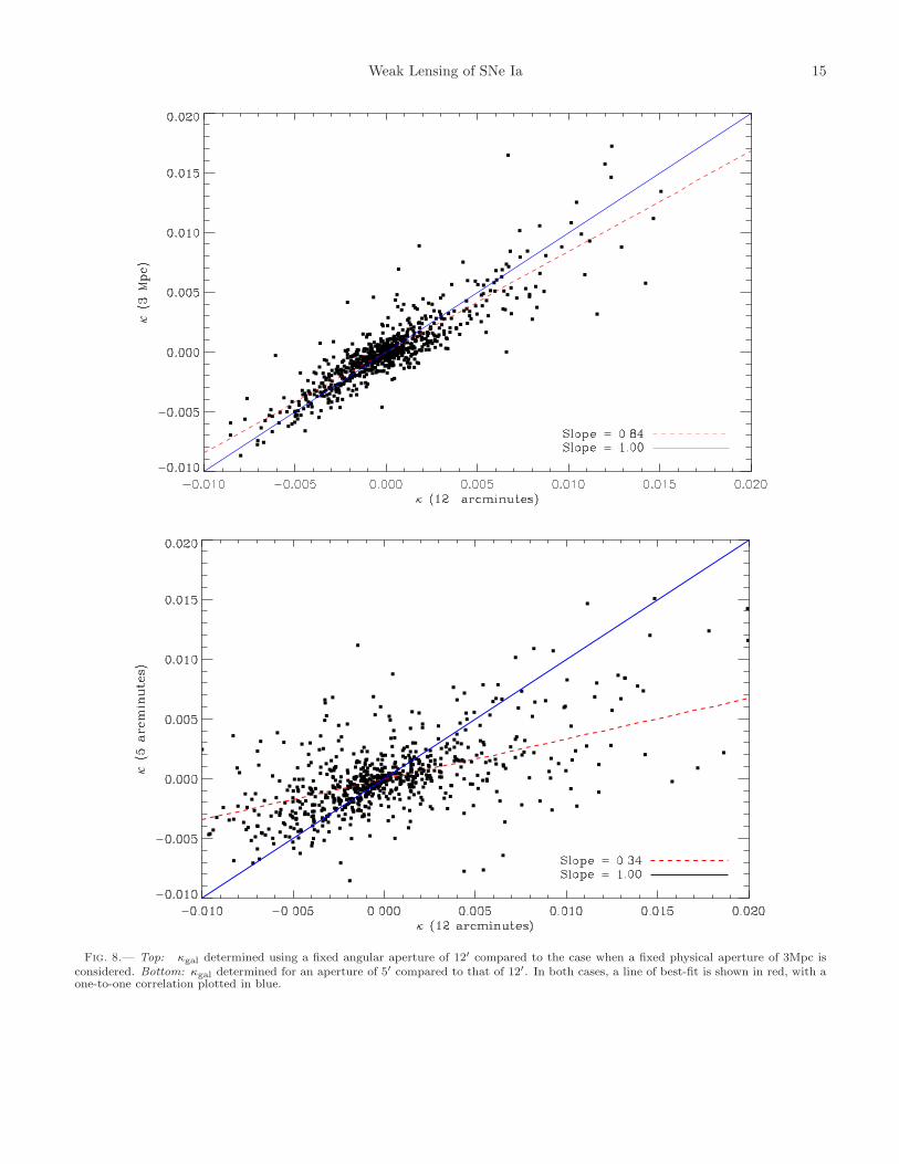
For an individual line-of-sight, we require a method for determining an aperture within which to count galaxies, inorder to describe the overdensity along that line-of-sight. In this appendix we investigate two approaches involvingfixed apertures around each SNe; we do not consider adaptive apertures here.First, we consider an aperture of fixed angular radius (e.g. (Williams and Song 2004)). This is easy to define,

but suffers from the fact that the transverse physical separation between a SN Ia and a foreground galaxy is a

14 Smith et al.

function of redshift. Secondly, we consider an aperture of fixed physical scale so that a galaxy of a fixed physicaltransverse separation from the SN light–of–light is included. In this second case, we need to define the cosmologicalbackground (in particular the Hubble constant, H0). For this test, we assume a flat Universe with Ωm = 0.3 andH0 = 73.8kms−1 Mpc−1 (Riess et al. 2011).We test the robustness of these two measurements against each other in Figure 8 (top panel). In this case, we have

compared a fixed angular aperture of 12 arcminutes and a fixed physical aperture of 3Mpc. The two estimates arestrongly correlated, with ρ = 0.86, indicating that either of these aperture measures will act as a similar proxy foroverdensity. We considered apertures from 8-15 arcminutes and 2-10Mpc and found a similar level of consistency.

B. OPTIMAL APERTURE SIZE

Having shown that our estimate of κgal is insensitive to the method used to determine the aperture, we now considerhow the aperture size considered affects the distribution of κgal. Smaller apertures are likely to be dominated byindividual galaxies while larger radii will trace the mean matter distribution. The bottom panel of Figure 8 shows theestimated value of κgal for two aperture radii; 5′ and 12′, respectively. The two distributions are strongly correlated,with r = 0.57, indicating that at these scales the recovered value of κgal is robust to the aperture size considered.We observe that in each case, κgal ∼ O(0.01), predicting a 1% lensing signal.Next, we consider the optimal aperture size for our data and measurement. Using the Spearman correlation coefficient

and the data shown on Figure 6, we re-calculate ρ as a function of the aperture size used to calculate κgal, which isthen correlated with the Hubble residuals (µobs−µcosmo). We fix the cosmological and supernova nuisance parametersas described in §4.4. In Figure 9, we show the value of ρ as a function of aperture size, and witness a clear “bump” inthe strength of the correlation between aperture sizes of 10 to 15 arcminutes, with the maximum near 12 arcminutes.This observed signal is consistent with the expected lensing prediction, with a negative correlation indicating that SNewith κgal > 0 are marginally brighter than those with κgal < 0, after correction. The reduction in the signal at largeraperture radii is due to these apertures picking up other structures which are not causing the SNe lensing.

C. EFFECT OF A MINIMUM REDSHIFT LIMIT

In §3 we enforced that only SNe Ia with z > 0.2 are included in our fiducial sample. In this appendix we considerthe implications that this cut has on our results. Using the Spearman correlation coefficient discussed and the datashown on Figure 6, we re-calculate ρ as a function of the minimum redshift used in the sample, which is then correlatedwith the Hubble residuals (µobs − µcosmo). We fix the cosmological and supernova nuisance parameters as describedin §4.4. In Figure 10, we shows the value of ρ as a function of minimum redshift, and observe a clear increase in thesignal with increasing redshift, indicating that SNe Ia at higher redshifts are more sensitive to the lensing signal, asexpected. However, with the increasing minimum redshift, the size of our the resulting sample decreases, increasingthe inferred uncertainties. A signal is observed independent of the redshift cut considered.

Weak Lensing of SNe Ia 15

Fig. 8.— Top: κgal determined using a fixed angular aperture of 12′ compared to the case when a fixed physical aperture of 3Mpc isconsidered. Bottom: κgal determined for an aperture of 5′ compared to that of 12′. In both cases, a line of best-fit is shown in red, with aone-to-one correlation plotted in blue.

16 Smith et al.

Fig. 9.— The Spearman’s rank correlation coefficient, ρ as a function of aperture radii considered, when a fixed angular size aperture isconsidered. The data has been smoothed, and is overplotted in red. The uncertainty in the correlation coefficient is shown as a blue band.

Fig. 10.— The Spearman’s rank correlation coefficient, ρ as a function of minimum redshift considered, when a fixed angular size apertureof 12 arcseconds is considered. The uncertainty in the correlation coefficient is shown as a blue band.