Athens - 11 May 2004 Statistics and Probability in Geosciences: Fernando Sansó DIIAR - Politecnico di Milano – Polo Regionale di Como from Least Squares

Athens - 11 May 2004

Statistics and Probability Statistics and Probability in Geosciences:in Geosciences:

Fernando Sansó

DIIAR - Politecnico di Milano – Polo Regionale di Como

from Least Squares from Least Squares to Random Fieldsto Random Fields


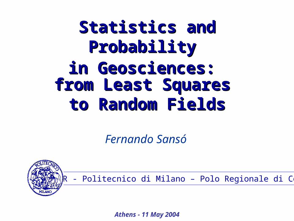
Statistics of GeosciencesStatistics of Geosciences

From the availability of new electronic HW, new impulses to model theory and field theory

JeffreysBaardaMoritzKrarup

Tarantola-ValletteGeman-Geman

LaplaceLegendre

GaussPoissonMarkov

Statistics drifts away from its origins, so much entangled with geo-sciences (and astronomy)


recognizing that Statistics is the art and science

of ambiguous knowledge,

I claim that the “whole probabilistic”,

Bayesian, point of view can be taken as a

unifying foundation for all spatial

information sciences.


Scientific concepts are born of an abstraction process, namely

when we observe natural phenomena, after eliminatinga multitude of tiny details, we can grasp the common and regular elements on which axioms rules and laws can be built.

(From Plato’s ideas () to Euclede’s () elements).


Examples

• a straight line; who has ever seen one?

• a Eucledean triangle: measuring its angles at the astronomical level has become one of the means to decide about the curvature of the universe;

• the Galilean equivalence principle, which emerges from physical experiments only by abstracting from friction, by assuming a constant gravity etc.


Psychologically one can understand why at the beginning of modern science the incertitude was considered as the enemy, classified as “measurement error”.

This is how modern statistics was born from the very beginning as “error theory”, based on a probabilistic interpretation via the central theorem and used in an inferential approach, to produce “best” estimates of the parameters of interest, according to a proto-maximum likelihood criterion.


Historical examples

• The astronomical measurement of Jupiter diameters to test the hypothesis that its figure was ellipsoidal and rotating around the minor axis.

• The geodetic measurements of arcs of meridians, performed by the French Academy in France, in Lapland and on the Andes, to measure the eccentricity of the Earth.


One fundamental step in the development of the understanding of statistics has been the clear establishment of the so called Gauss-Markov linear standard model, with all its developments in least squares theory: this is understood by explaining what are

• the deterministic model,

• the stochastic model.


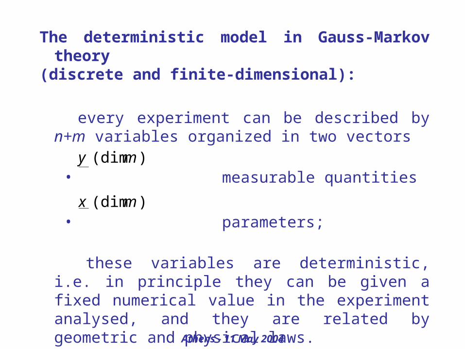
The deterministic model in Gauss-Markov theory

(discrete and finite-dimensional):

every experiment can be described by n+m variables organized in two vectors

• measurable quantities

• parameters;

these variables are deterministic, i.e. in principle they can be given a fixed numerical value in the experiment analysed, and they are related by geometric and physical laws.

)(dimmy

)(dimmx


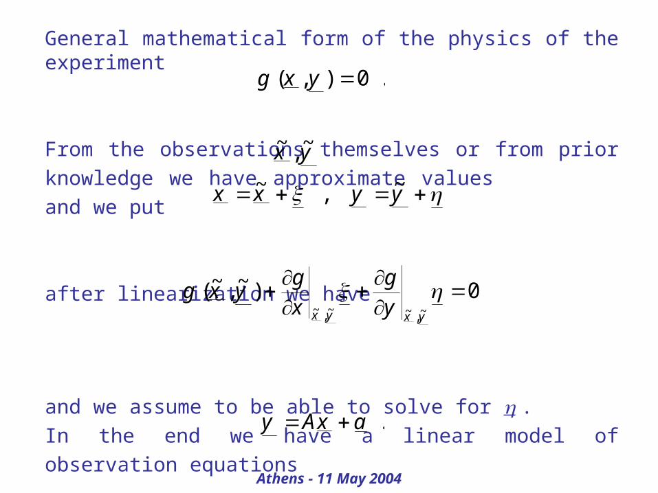
General mathematical form of the physics of the experiment

From the observations themselves or from prior knowledge we have approximate values and we put

after linearization we have

and we assume to be able to solve for .In the end we have a linear model of observation equations

.0),( yxg

yx ~,~

yyxx ~,~

0)~,~(~,~~,~

yxyx yg

xg

yxg

.axAy


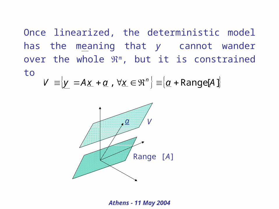
Once linearized, the deterministic model has the meaning that y cannot wander over the whole m, but it is constrained to

][Range, AaxaxAyV n

Range [A]

Va


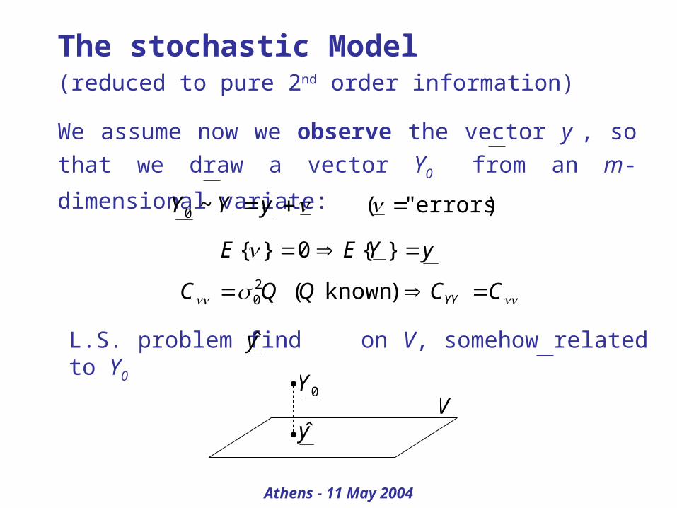
The stochastic Model (reduced to pure 2nd order information)

We assume now we observe the vector y , so that

we draw a vector Y0 from an m-dimensional

variate: )errors""(~0 yYY

yYEE }{0}{

CCQQC YY )known(20

L.S. problem find on V, somehow related to Y0 y

y

0YV


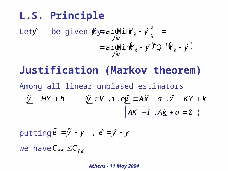
L.S. Principle

Let be given by:

Justification (Markov theorem)

Among all linear unbiased estimators

2

0ˆ

1ˆMinargˆQ

VyyYyy

hYHy ~ kYKxaxAyVy ~,~~ i.e.,~(

)0, akAIAK

yYQyYVy

ˆˆMinarg 01

0ˆ

yyeyye ˆˆ,~~putting

we have .~~ˆˆ eeee CC


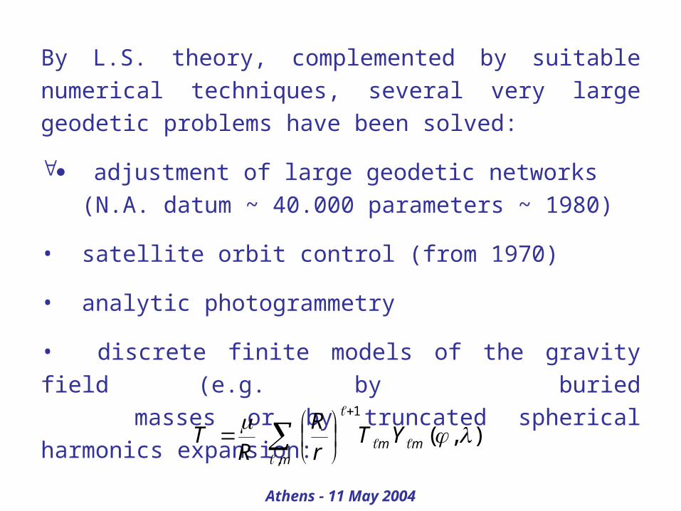
By L.S. theory, complemented by suitable numerical techniques, several very large geodetic problems have been solved:

adjustment of large geodetic networks (N.A. datum ~ 40.000 parameters ~ 1980)

• satellite orbit control (from 1970)

• analytic photogrammetry

• discrete finite models of the gravity field (e.g. by buried masses or by truncated spherical harmonics expansion:

),(,

1

mm

m

YTrR

RT


From L.S. theory new problems have evolved:

• testing theory as applied to Correctness of the model (2 test on ) Values of the parameters (significance of input factors in linear regression analysis)

Outliers identification and rejection (Baarda’s data snooping) and the natural evolution towards robust estimators (L1-estimators etc.)

20


Mixed models with two types of parameters x (continuous), b (integers) like with GPS observations where b are initial phase ambiguities.

Note: the numerical complexity if we adopt a simple trial and error strategy for b; if we have a base line with 10 visible satellites and for each double difference we want to try 3 values, we have to perform

39 ~ 20.000adjustments.


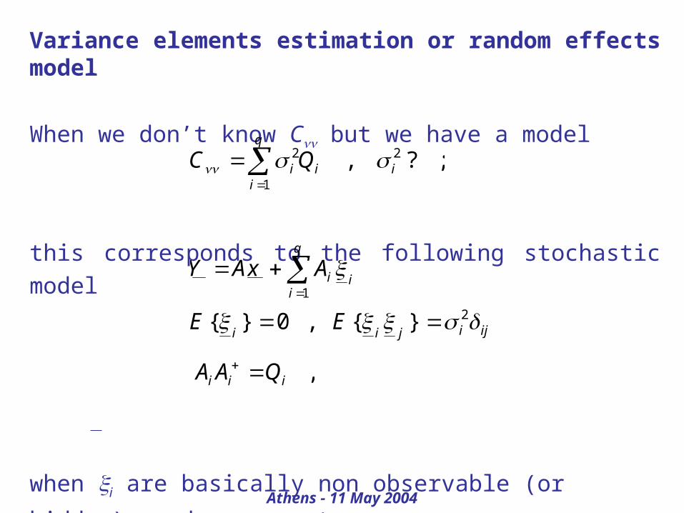
Variance elements estimation or random effects model

When we don’t know C but we have a model

this corresponds to the following stochastic model

when i are basically non observable (or hidden)

random parameters.

;?, 2

1

2i

q

iii QC

q

iiiAxAY

1

ijijiiEE 2}{,0}{

,iii QAA


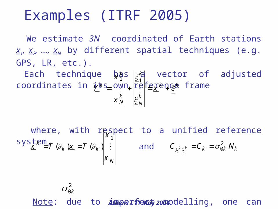
Examples (ITRF 2005)

We estimate 3N coordinated of Earth stations x1, x2, …,

xN by different spatial techniques (e.g. GPS, LR, etc.).

Each technique has a vector of adjusted coordinates in its own reference frame

where, with respect to a unified reference system,

Note: due to imperfect modelling, one can assume that the estimate of is unrealistic.

20k

kk

kN

k

kN

k

k x

x

x

Y

11

N

kkk

x

x

TxTx 1

)()( and kkk NCC kk20


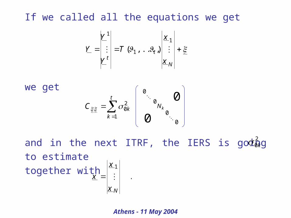
If we called all the equations we get

we get

and in the next ITRF, the IERS is going to estimate together with

N

tt x

x

T

Y

Y

Y 1

1

1

),...,(

t

kkC

1

20

0

0

0

0

0

0kN

.1

Nx

x

x

20k


The Bayesian revolution

• Probability is an axiomatic index measuring the subjective state of knowledge of a certain system,

• every system is thus described by a number of random variables through their joint distribution,

• every observation modifies the state of knowledge of the system, namely the distribution of the relevant variables, through the operation of probabilistic conditioning.


According to this vision, the physical laws are

only verified in the mean, when we average on a

population of effects that cannot be controlled,

and which can be described only by a probability

distribution, expressing our prior knowledge of

the phenomenon.

(De Finetti)


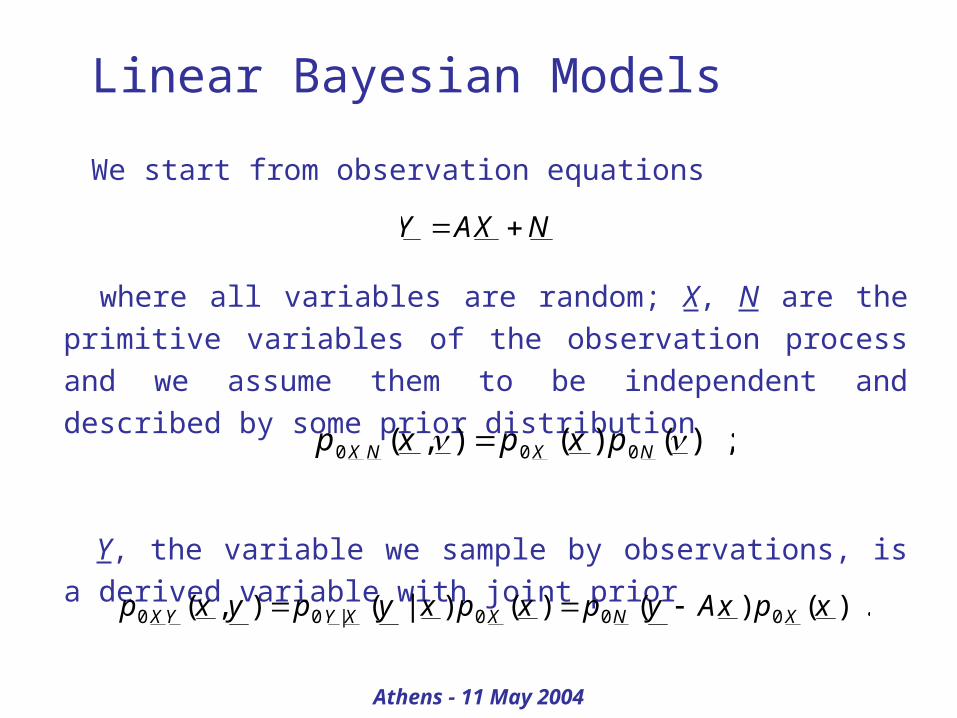
Linear Bayesian Models

We start from observation equations

where all variables are random; X, N are the primitive variables of the observation process and we assume them to be independent and described by some prior distribution

Y, the variable we sample by observations, is a derived variable with joint prior

NXAY

;)()(),( 000 NXNX pxpxp

.)()()()|(),( 000|00 xpxAypxpxypyxp XNXXYYX


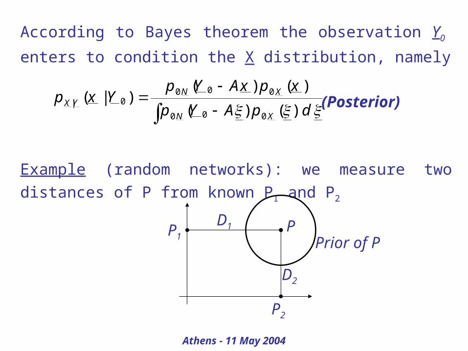
According to Bayes theorem the observation Y0 enters

to condition the X distribution, namely

(Posterior)

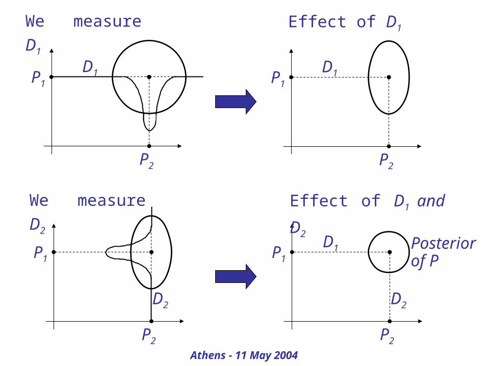
Example (random networks): we measure two

distances of P from known P1 and P2

dpAYp

xpxAYpYxp

XN

XNYX

)()(

)()()|(

000

0000|

PP1

P2

D1

D2

Prior of P


P1

P2

D1 P1

P2

D1

P1

P2

D2

P1

P2

D1

D2

We measure

D1

Effect of D1

We measure

D2

Effect of D1 and D2

Posteriorof P


A general Bayesian network is a network where

points are random and measurements change

their distribution; in a sense (apart from

Heisenberg’s principle) there is a striking similarity

with quantum theory.

Let us now restrict the Bayes concept to the linear

regression case.


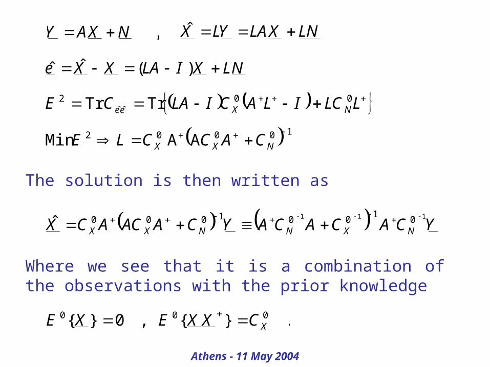
,NXAY LNXLAYLX ˆ

NLXILAXXe )(ˆˆ

LLCILACILACE NXee00

ˆˆ2 TrTr

10002 AAMin NXX CACCLE

The solution is then written as

Where we see that it is a combination of the observations with the prior knowledge

YCACACAYCAACACX NXNNXX

111 01

001000ˆ

.}{,0}{ 000XCXXEXE


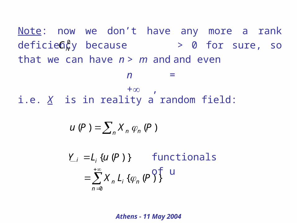
Note: now we don’t have any more a rank deficiency because > 0 for sure, so that we can have n > m and and even

0NC

n = + ,

i.e. X is in reality a random field:

n nn PXPu )()(

)}({ PuLY ii

)}({0

PLX nin

n

functionals of u


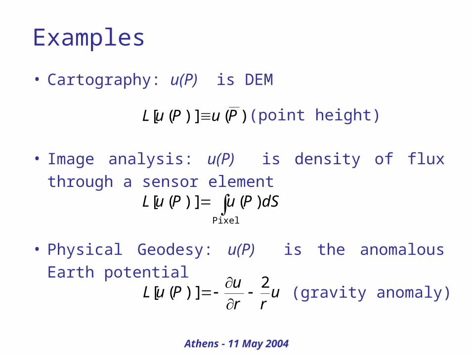
Examples

• Cartography: u(P) is DEM

• Image analysis: u(P) is density of flux through a sensor element

• Physical Geodesy: u(P) is the anomalous Earth potential

)()]([ PuPuL (point height)

dSPuPuL Pixel

)()]([

urr

uPuL

2)]([

(gravity anomaly)


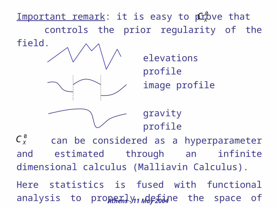
Important remark: it is easy to prove that controls the prior regularity of the field.

elevations profile

0XC

image profile

gravity profile

can be considered as a hyperparameter and estimated through an infinite dimensional calculus (Malliavin Calculus).

Here statistics is fused with functional analysis to properly define the space of estimators.

0XC


Conclusions

If modern statistics, which was born at the

beginning together with geodesy and astronomy

to treat measurement errors, has slowly drifted

away to become mate of mechanics, then of radio-

signals analysis and finally of economic sciences,

nowadays we are entitled to say that Earth

sciences with their need of estimating spatial

fields, are giving to statistics a serious scientific

contribution, pushing it along the road of modern

probability theory and functional analysis.

Documents

Athens - 11 May 2004 Statistics and Probability in Geosciences: Fernando Sansó DIIAR - Politecnico di Milano – Polo Regionale di Como from Least Squares