Embed Size (px)
Citation preview
ATL
AS-
CO
NF-
2016
-020
11/0
4/20
16
ATLAS NOTEATLAS-CONF-2016-020
11th April 2016
Search for four-top-quark production in final states with onecharged lepton and multiple jets using 3.2 fb−1 of proton-protoncollisions at
√s = 13 TeV with the ATLAS detector at the LHC
ATLAS Collaboration
Abstract
A search for four-top-quark production, tt̄tt̄, is presented based on the proton-proton collisiondata taken at
√s = 13TeVand collectedwith theATLASdetector at theLargeHadronCollider
during 2015, corresponding to an integrated luminosity of 3.2 fb−1. Data are analysed inthe single-lepton channel, characterised by an isolated high transverse momentum electronor muon and multiple jets. The search exploits the high jet multiplicity, high b-taggedjet multiplicity and large total sum of jet transverse momenta which characterise signalevents and provide good discrimination against the dominant background from top-quarkpair production in association with jets. Events are categorised according to their jet andb-tagged jet multiplicities in order to improve the sensitivity of the search and reduce theimpact of systematic uncertainties. No significant excess of events above the backgroundexpectation is found and an observed (expected) upper limit of 21 (16) times the four-top-quark Standard Model cross-section is obtained at 95% confidence level. Additionally, upperbounds on four-top-quark production are set in different scenarios of physics beyond theStandard Model.
11 April 2016: references updated
© 2016 CERN for the benefit of the ATLAS Collaboration.Reproduction of this article or parts of it is allowed as specified in the CC-BY-4.0 license.
1. Introduction
The Large Hadron Collider (LHC) proton-proton (pp) collision centre-of-mass energy was increased to√
s = 13 TeV in 2015, opening a unique window to search for signatures with mass scales higher thanever before and involving several high-mass particles. One attractive possibility is to focus on the heaviestknown elementary particle described by the Standard Model (SM), the top quark [1]. With a mass closeto the scale of electroweak symmetry breaking, the top quark is predicted to have a very large couplingto the Higgs boson and in many physics models beyond the Standard Model (BSM) also to other newresonances [2–5]. Possible new phenomena may enhance the SM cross-sections through the productionof heavy objects in association with a top-quark pair. Measurements of the production of tt̄ pairs inassociation with photons [6], W or Z bosons [7, 8], and additional heavy-flavour jets [9–11] were found tobe in good agreement with the SM prediction. A small excess is observed in the production of the Higgsboson in association with a tt̄-pair [12]. An enhanced rate for events containing many top quarks [13,14], and in particular events containing four top quarks, tt̄tt̄, can be a sign of new phenomena [15–21].This note focuses on the search for four-top-quark production and targets resolved topologies.1 Thisincludes four-top-quark production with the SM kinematics, as well as several BSM models consideredas benchmarks: tt̄tt̄ production via four-top-quarks contact interaction [21] and from universal extradimensions scenarios [20, 22].
Searches for four-top-quark production using the Run 1 dataset at√
s = 8 TeV were performed both by theATLAS [23, 24] and CMS [25, 26] collaborations, with no observed excess of data above the backgroundexpectation. At
√s = 13 TeV, the SM four-top-quark production cross-section (σSM
t t̄t t̄) increases by a factor
of 9 compared to√
s = 8 TeV, and in next-to-leading order (NLO) perturbation theory is predicted tobe σSM
t t̄t t̄≈ 9.2 fb, with relative scale and parton distribution function (PDF) uncertainties of the order
of 30% and 6%, respectively [27, 28]. The final state topology of a four-top-quark event is determinedby the decays of each of the W -bosons, assuming that the top quark decays exclusively through t → W b[29]. Depending on the W -boson decay mode, there are 35 different final states which can be groupedinto 4 classes of channels, each one with a different signature: fully hadronic (with a branching ratio(BR) of ∼ 20.9%), single-lepton (BR ∼ 40%), dilepton (BR ∼ 28.8%) and multi-lepton (BR ∼ 10.3%).The four-top-quark decay topology considered in this search corresponds to single-lepton events with oneisolated lepton (electron or muon).
The search presented in this note exploits the high jet multiplicity (up to 10 resolved jets), high b-tagged jetmultiplicity (up to 4 b-tagged jets) and large total sum of jet transverse momenta which characterise signalevents. The main source of background to this search comes from top-quark pairs produced in associationwith additional jets. Selected events are classified into several categories according to their jet and b-tagged jet multiplicities in order to improve the sensitivity of the search and constrain uncertainties on thebackground prediction. Although this analysis technique results in a relatively high signal-to-backgroundratio, a statistically significant observation of the rare SM four-top-quark process is not expected usingthe dataset recorded so far by the ATLAS experiment. However, as mentioned above, a variety of newphysics models predict enhancements to σSM
t t̄t t̄. Hence, any deviation from the SM prediction will provide
supporting evidence for BSM physics, while setting upper limits on BSM production cross-sections willconstrain such theories.
1 In the resolved topology, the top quark decay products are well-separated and individually reconstructed objects.
2
2. ATLAS Detector
The ATLAS detector [30] at the LHC is a multi-purpose particle detector with a forward-backwardsymmetric cylindrical geometry and nearly 4π coverage in solid angle2. It consists of an inner trackingdetector (ID), electromagnetic and hadronic calorimeters, and a muon spectrometer. The inner detector,including the newly-installed insertable B-layer [31], provides charged particle tracking information fromsilicon pixel and microstrip detectors in the pseudorapidity region |η | < 2.5, surrounded by a transitionradiation tracker, which enhances electron identification properties in the region |η | < 2.0. The ID issurrounded by a thin superconducting solenoid providing an axial 2 T magnetic field and by a fine-granularity lead/liquid-argon electromagnetic calorimeter covering |η | < 3.2, which provides energymeasurements of electromagnetic showers. Hadron calorimetry employs the sampling technique, witheither scintillator tiles or liquid argon as active media, and with steel, copper, or tungsten as absorbermaterial. The calorimeters cover |η | < 4.9. An extensive muon spectrometer with an air-core toroidmagnet system surrounds the calorimeters. Three layers of high-precision tracking chambers providecoverage in the range |η | < 2.7 and are located in a toroidal field of approximately 0.5 T and 1 T inthe central and end-cap regions of ATLAS, respectively. A two-level trigger system [32], using customhardware followed by a software-based level, is used to reduce the event rate to a maximum of around 1kHz for offline storage.
3. Object reconstruction and event selection
The final states considered in this search require the presence of one charged lepton candidate (electronor muon) and multiple hadronic jets. Events are required to pass single-electron or single-muon triggerswith transverse-momentum thresholds at 24 GeV in the case of electrons and 20 GeV in the case of muons.In addition, events are asked to have at least one reconstructed vertex, that is required to have at leasttwo tracks with pT > 0.4 GeV and to be consistent with the beam-collision region in the x – y plane. Ifmultiple vertices are reconstructed, the vertex with the largest sum of the squared transverse momenta ofits associated tracks is taken as the primary vertex. For the final states considered in this analysis, thevertex reconstruction and selection efficiency is close to 100%.
Electron candidates are reconstructed [33–35] froman isolated electromagnetic calorimeter energy deposit,matched to an ID track, within the fiducial region of |ηcluster | < 2.47, where ηcluster is the pseudorapidityof the calorimeter energy deposit associated with the electron candidate. Candidates within the transitionregion between the barrel and end-cap electromagnetic calorimeters, 1.37 < |ηcluster | < 1.52, are excluded.The electron candidates are required to be isolated from additional tracks within a cone around theirdirections with a radius of ∆R ≡
√(∆η)2 + (∆φ)2 = min(0.2, 10 GeV/pT) [36], such that the sum of the
transverse momenta of the tracks within that cone is less than 6% of the electron pT.
Muon candidates are reconstructed [37] by combining matching tracks reconstructed in both the ID andthe muon spectrometer, using the complete track information of both detectors and accounting for materialeffects of the ATLAS detector structure. The muon candidates are required to be in the central region of
2 ATLAS uses a right-handed coordinate system with its origin at the nominal interaction point (IP) in the centre of the detector.The positive x-axis is defined by the direction from the IP to the centre of the LHC ring, with the positive y-axis pointingupwards, while the beam direction defines the z-axis. Cylindrical coordinates (r, φ) are used in the transverse plane, φ beingthe azimuthal angle around the z-axis. The pseudorapidity η is defined in terms of the polar angle θ by η = − ln tan(θ/2).
3
|η | < 2.5 and to be isolated using the same track-based variable as for electrons, except that the maximum∆R in this case is 0.3.
Moreover, both electrons andmuons arematched to the primary vertex by requiring the longitudinal impactparameter, z0, to satisfy |z0 sin θ | < 0.5 mm, where θ is the polar angle of the track.3 The significance ofthe transverse impact parameter calculated with respect to the measured beam line position is required tosatisfy |d0/σ(d0) | < 5 for electrons and |d0/σ(d0) | < 3 for muons, where σ(d0) is the uncertainty ond0.
Jets are reconstructed from three-dimensional topological energy clusters [38] in the calorimeter usingthe anti-kt jet algorithm [39] with a radius parameter of 0.4. Each topological cluster is calibrated to theelectromagnetic energy scale prior to jet reconstruction. The reconstructed jets are then calibrated to theparticle-level by the application of a jet energy scale (JES) derived from simulation and in situ correctionsbased on Run 1 data [40] and checked with early Run 2 data [41]. Quality criteria are imposed to identifyjets arising from non-collision sources or detector noise and any event containing at least one such jet isremoved [42]. To reduce the contribution from jets associated with pileup, jets with pT < 50 GeV and|η | < 2.4 are required to pass a pileup rejection criterion, the jet vertex tagger [43], based on track-basedvariables. In order to avoid double-counting of electron energy deposits as jets, the closest jet within∆R < 0.2 from a selected electron is removed. If the nearest jet surviving the above selection is within∆R < 0.4 of an electron, the electron is discarded to ensure that selected electrons are sufficiently separatedfrom nearby jet activity. In case an electron shares a track with a selected muon, the electron is removed.To reduce the background from muons from heavy-flavour decays inside jets, muons are removed if theyare separated from the nearest jet by ∆R < 0.4. However, if this jet has fewer than three associatedtracks, the muon is kept and the jet is removed instead, avoiding an inefficiency for high-energy muonsthat undergo significant energy loss in the calorimeters.
To identify jets containing b-hadrons (henceforth referred to as b-jets), a multivariate discriminant is usedwhich combines information on the impact parameters of inner detector tracks associated to the jet, thepresence of displaced secondary vertices, and the reconstructed flight paths of b- and c-hadrons inside thejet [44–46]. Jets are considered as being b-tagged if the value of the multivariate discriminant is largerthan a certain threshold. In this search, the working point corresponding to approximately 77% b-taggingefficiency for b-jets in simulated tt̄ events is chosen, although the exact efficiency varies with pT. Thetagging algorithm gives a rejection factor of about 126 against light quark and gluon jets, and about 4.5against jets originating from charm quarks [47].
Events of interest are retained if they contain exactly one identified electron or muon with pT > 25 GeVand at least five jets with pT > 25 GeV satisfying the quality and kinematic criteria discussed above, atleast two of which must be b-tagged. Events having a second lepton with pT larger than 25 GeV arevetoed. In the following and unless stated otherwise, only events satisfying this selection, referred to as“preselection”, are considered.
After event preselection, the main background processes come from the SM production of tt̄+jets andsingle top quarks, as well as W - or Z-boson production in association with jets. Small contributions arisefrom the associated production of a vector boson V (V = W, Z) or a Higgs boson and a tt̄ pair (tt̄ + Vand tt̄ + H) and from diboson (WW , W Z , Z Z) production. Multijet events also contribute to the selectedsample via the misidentification of a jet or a photon as an electron or the presence of a non-prompt electronor muon.
3 The longitudinal impact parameter z0 is the difference between the longitudinal position of the track along the beam line atthe point where the transverse impact parameter (d0) is measured and the longitudinal position of the primary vertex.
4
4. Data sample, signal simulation and background modelling
The search is performed with the 2015√
s = 13 TeV pp collision data sample with 25 ns bunch spacingcollected by the ATLAS experiment between August and November 2015, corresponding to an integratedluminosity of 3.2±0.2 fb−1. The uncertainty is derived following the samemethodology as that detailed inRef. [48]. The peak delivered instantaneous luminosity during this period reachedL = 5.2×1033cm−2s−1
and the average number of interactions per pp bunch crossing ranged from approximately 5 to 25, witha mean of 14. The data are only used if they were recorded during stable beam conditions and with allrelevant ATLAS detector subsystems operational.
Monte-Carlo simulation samples (MC) are used tomodel the expected signal and background distributions.TheMC samples were processed either through the full ATLAS detector simulation [49] based onGeant4[50] or through a faster simulationmaking use of parametrised showers in the calorimeters [51]. Additionalsimulated pp collisions generated using Pythia-8.186 [52] were overlaid to model the effects of both in-and out-of-time pileup from additional pp collisions in the same and nearby bunch crossings. Thedistribution of the number of additional pp interactions in the MC samples is reweighted to match the oneobserved in data. All simulated samples were processed through the same reconstruction algorithms andanalysis chain as the data. The heavy flavour decays, particularly important to this search, were modelledusing the EvtGen [53] program, except for processes modelled using the Sherpa generator [54].
4.1. Signal modelling
Simulated events for the main signal process, i.e. the four-top-quark production with SM kinematics, aregenerated with the [email protected] [28] leading-order (LO) generator and the NNPDF2.3LO PDF set [55], interfaced to Pythia-8.186 using the A14 tune [56].
This search also sets upper bounds on different BSM models, particularly on tt̄tt̄ production via four-top-quark contact interaction (CI) and from Universal Extra Dimensions (UED) scenarios [20, 22]. A classof models involving new heavy vector particles strongly coupled to the right-handed top quark [57], suchas top quark compositeness [16, 58, 59] or Randall–Sundrum extra dimensions [17], can be described viaan effective field theory (EFT) involving a four-fermion CI [21]. The Lagrangian assumed is:
L4t =|C4t |
Λ2 (t̄RγµtR)(t̄RγµtR), (1)
where tR is the right-handed top quark spinor, γµ are the Dirac matrices, C4t is the coupling constant, andΛ is the mass scale of BSM physics. In addition, a specific UEDmodel involving new heavy particles withtwo extra dimensions that are compactified using the geometry of the real projective plane (2UED/RPP)is considered [22]. The compactification of the extra dimensions leads to discretisation of the momentaalong their directions. The model is parametrised by the radii R4 and R5 of the extra dimensions or,equivalently, by mKK = 1/R4 and ξ = R4/R5. This model predicts the pair production of tier4 (1,1)Kaluza–Klein excitations of the heavy photon A(1,1)
µ with mass approximately√
2mKK that decay into SMtt̄-pairs with a branching ratio assumed to be 100% [20]. Final states from 2UED/RPP events with thisassumption contain tt̄tt̄ + n light jets + n′ leptons, with n = 2, 3, 4 and n′ = 0, 2, 4. The samples withthe EFT and 2UED/RPP models are generated with the Madgraph5_aMC@NLO [28] LO generator (theversions used are 2.2.3 and 2.2.2 for EFT and 2UED/RPP, respectively) and the NNPDF2.3 LO PDF set,
4 A tier of Kaluza–Klein towers is labelled by two integers, corresponding to the two extra dimensions with sizes πR4 and πR5.
5
interfaced to Pythia8 (the versions used are 8.205 [60] and 8.186 for EFT and 2UED/RPP, respectively)using the A14 tune. In the case of the 2UED/RPP model, samples are generated with five different valuesof mKK (1 to 1.8 TeV in steps of 200 GeV) and theBridge [61] generator is used to decay the pair-producedexcitations from tier (1,1) generated by Madgraph5_aMC@NLO.
4.2. Background modelling
The tt̄+jets events are generated with Powheg-Box v2 [62–65], which provides a NLO accuracy inQCD with respect to the tt̄ process (using the CT10 PDF set [66]), interfaced to Pythia-6.428 [67]with the CTEQ6L PDF set [68] and the PERUGIA2012 underlying event (UE) tune [69]. The hardprocess factorisation scale µ f and renormalisation scale µr are set to the default Powheg value: µ =
(m2t + p2
T,top)1/2, where mt and pT,top are the top quark mass and transverse momentum evaluated forthe underlying Born configuration, respectively. The Powheg model resummation damping parameterhdamp, which controls matrix element to parton shower matching in Powheg and effectively regulates thehigh-pT radiation, is set to mt = 172.5 GeV, a setting which was found to best describe the tt̄ system pT at√
s = 7 TeV [70]. The sample is generated assuming a top quark mass of 172.5 GeV and top quark decaysexclusively through t → W b.
Several alternative tt̄ samples are produced with the goal of assessing modelling uncertainties for thisprocess. To provide a comparison to a different parton shower model, an alternative tt̄ sample is generatedusing the same Powheg model setup as for the nominal Powheg-Box v2 + Pythia-6.428 sample,while parton shower (PS), hadronisation, UE and multiple parton interactions (MPI) are simulated withHerwig++ (version 2.7.1) [71] with the UEEE5 tune [72] and the corresponding CTEQ6L1 PDF set. Toassess the systematic uncertainties related to the use of different models for the hard scattering generationwhile maintaining the same parton shower model, a sample using [email protected] [28]interfaced to Herwig++ 2.7.1 is generated. The effects of initial- and final-state radiation (ISR/FSR)are explored using two alternative Powheg-Box v2 + Pythia-6.428 samples, one with hdamp set to 2mt ,the renormalisation and factorisation scales set to half the nominal value and using the PERUGIA2012high-variation UE tune, giving more radiation, and one with the PERUGIA2012 low-variation UE tune,hdamp = mt and the renormalisation and factorisation scales set to twice the nominal value, giving lessradiation [73]. The µr and µ f scale variations and the hdamp variations are kept correlated since the twoproposed variations cover the full set of uncertainties obtained by changing the scales and the resummationdamping parameter independently.
The tt̄+jets samples are normalised to the theoretical cross-section value for the inclusive tt̄ process of832+46
−51 pb obtained with Top++ [74], performed at next-to-next-to-leading order (NNLO) in QCD andincluding resummation of next-to-next-to-leading logarithmic (NNLL) soft gluon terms [75–79].
The tt̄+jets samples are generated inclusively, but events are categorised depending on the flavour contentof additional particle jets in the event, i.e. jets not labelled as originating from the decay of the tt̄ system,as reported in Ref. [80] and described in the following. Particle jets are reconstructed by clustering stableparticles5 excluding muons and neutrinos with the anti-kt algorithm with a radius parameter of 0.4 andare required to have pT > 15 GeV and |η | < 2.5. Events where at least one such particle jet is matchedwithin ∆R < 0.4 to a b-hadron with pT > 5 GeV and not matched within ∆R < 0.4 to any of the partonsdirectly coming from the decay of a top quark are labelled as tt̄ + bb̄ events. Similarly, events whichare not labelled already as tt̄ + bb̄ where at least one such particle jet is matched within ∆R < 0.4 to a
5 A particle is considered stable if cτ ≥ 1 cm.
6
c-hadron with pT > 5 GeV and not matched within ∆R < 0.4 to any of the partons directly coming fromthe decay of a W boson are labelled as tt̄ + cc̄ events. Events labelled as either tt̄ + bb̄ or tt̄ + cc̄ aregenerically referred to below as tt̄+HF events, where HF stands for “heavy-flavour”. The remaining eventsare labelled as tt̄+light events, including those with no additional jets. A finer categorisation of differenttopologies in tt̄+HF, for example, two particle jets matched to an extra b-hadron or c-hadron each, a singleparticle jet matched to a single b-hadron or c-hadron, or a single particle jet matched to a b-hadron orc-hadron pair, is made for the purpose of comparing the different tt̄ event generators and the propagationof the systematic uncertainties related to the modelling of tt̄+HF.
The modelling of the tt̄ + bb̄ background, particularly important for the searches described in this note,is improved by reweighting the Powheg-Box v2 + Pythia-6.428 prediction to a dedicated prediction atNLO accuracy in QCD for tt̄ + bb̄ including parton showering [81], based on Sherpa + OpenLoops [54,82] using the CT10 PDF set. The reweighting is done at generator level using several kinematic variablessuch as the top quark pT, tt̄ system pT, and the ∆R of the jet pair not coming from the top-quark decays andtheir combined pT, following the same procedure as in Ref. [80] but using an updated prediction at
√s =
13 TeV. It is performed for the different topologies of tt̄ + bb̄ in such a way that the inter-normalisationof each of the categories and the relevant kinematic distributions are at NLO accuracy in QCD. Afterthe reweighting, the modelling of the relevant kinematic variables in each category is found to be inreasonable agreement between the reweighted Powheg-Box v2 + Pythia-6.428 prediction and Sherpa +OpenLoops.
Samples of W/Z+jets events are generated with the Sherpa-2.1.1 [54] generator. The matrix-elementcalculation is performed with up to 2 partons at NLO in QCD and up to 4 partons at LO using Comix [83]andOpenLoops [82]. The matrix element calculation is merged with the Sherpa parton shower [84] usingthe ME+PS@NLO prescription [85]. The PDF set used for the matrix-element calculation is CT10 witha dedicated parton shower tuning developed by the Sherpa authors. The W+jets and Z+jets samples arenormalised to the W and Z inclusive production NNLO theoretical cross-sections in QCD respectively,calculated with FEWZ [86].
Samples of single top quark backgrounds corresponding to the Wt and s-channel production mechanismsare generated with Powheg-Box v2 [62–65] using the CT10 PDF set. Overlaps between the tt̄ and Wtfinal states are removed using the “diagram removal” scheme [87]. Samples of t-channel single top quarkevents are generated using the Powheg-Box v1 [88] NLO generator that uses the 4-flavour scheme. Thefixed four-flavour PDF set CT10f4 [66] is used for the matrix-element calculations. The single top quarksamples are normalised to the approximate NNLO theoretical cross-sections [89–91]. The parton shower,hadronisation and underlying event are modelled using Pythia-6.428 with the PERUGIA2012 tune.
Diboson processes with one of the bosons decaying hadronically and the other leptonically are simulatedusing the Sherpa-2.1.1 generator [54]. They are calculated for up to 1 (Z Z) or 0 (WW , W Z) additionalpartons at NLO and up to 3 additional partons at LO using the same procedure as forW/Z+jets. The CT10PDF set is used in conjunction with dedicated parton shower tuning of the Sherpa fragmentation model.All diboson samples are normalised to their NLO theoretical cross-sections provided by Sherpa.
Samples of tt̄+V (withV =W and Z , including non-resonant Z/γ∗ contributions and tt̄+WW production)are generated at LO with [email protected] and interfaced to the Pythia-8.186 partonshower model with the A14 NNPDF2.3 UE tune [56]. The tt̄ +W and tt̄ + Z processes are generated withup to two additional partons in the matrix element. No additional partons are included in the tt̄ +WWgeneration. The tt̄ + V events are normalised to their NLO cross-section [28]. A sample of tt̄ + H eventsis generated with the [email protected] generator using the CT10 PDF set. Showering is
7
performed using Herwig++-2.7.1 [71] and the UEEE5 [72] tune with the CTEQ6L1 PDF set. Inclusivedecays of the Higgs boson are assumed in the generation of the tt̄ + H sample, which is normalised tocross-section calculated at NLO [92, 93].
Table 1 provides a summary of basic parameters of the MC samples used in the search. An overallsummary of the validation of MC event generators and MC simulation setups of W/Z+jets, multi-boson,top quark, tt̄ + V and tt̄ + H productions in the ATLAS experiment can be found in Refs. [94–98].
Process Generator Tune PDF set Inclusive cross-section+ fragmentation/hadronisation order in pQCD
t t̄ t t̄ SM [email protected] A14 NNPDF2.3 NLO+ Pythia-8.186
t t̄ + jets Powheg-Box v2 PERUGIA2012 CT10 NNLO+NNLL+ Pythia-6.428
Single top Powheg-Box v2 PERUGIA2012 CT10 NNLO+NNLL+ Pythia-6.428
t t̄ +W/Z/WW [email protected] A14 NNPDF2.3 NLO+ Pythia-8.186
t t̄ + H [email protected] UEEE5 CT10 NLO+ Herwig++-2.7.1
Dibosons Sherpa-2.1.1 Default CT10 NLOWW , W Z , Z Z
W /Z + jets Sherpa-2.1.1 Default CT10 NNLO
Table 1: List of generators used for the different background processes. Information is given about the perturbativeQCD (pQCD) highest-order accuracy used for the normalisation of the different samples, the underlying event tunesand PDF sets considered. All processes but tt̄tt̄ and tt̄ +W/Z/WW are generated at NLO in QCD.
4.3. Estimation of non-prompt and fake lepton backgrounds
Non-prompt leptons, hadrons and photons may satisfy the selection criteria, giving rise to so called “non-prompt and fake” lepton backgrounds (NP & fakes). In this search, the multijet background normalisationand shape are estimated directly from data using the matrix method technique [99, 100]. The methodexploits the differences in lepton identification-related properties between prompt, isolated leptons fromW -and Z-boson decays and thosewhere the leptons are either non-isolated or result from themis-identificationof photons or jets. Systematic uncertainties on the estimate are assessed using alternative control samples,propagating systematic uncertainties associated to object reconstruction and MC simulation to the fakelepton estimate as well as by comparing different parametrisations of the efficiencies, resulting in a totalnormalisation uncertainty of around 50%.
8
5. Analysis strategy and statistical interpretation
Signal events from SM four-top-quark production with single-lepton decay topology, where each partoncoming from a top quark or a W -boson decay can give rise to a separate jet (the so called “resolved”lepton-plus-jets final state), is characterised by the presence of 10 non-overlapping high-pT jets, out ofwhich 6 are light- and 4 are b-quark jets, one charged lepton and missing transverse momentum fromthe escaping neutrino. However, the limited detector acceptance and the b-tagging efficiency need to betaken into account. In order to calibrate the background prediction and constrain the related systematicuncertainties in signal-depleted channels with lower jet and b-tagged jet multiplicities, events are classifiedin several signal, control and validation regions. This maximises the sensitivity of the search.
5.1. Classification of event topologies
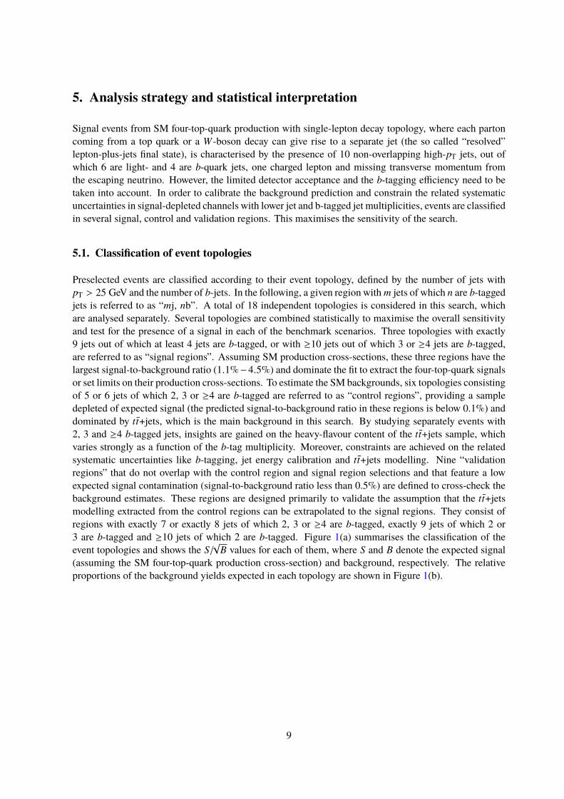
Preselected events are classified according to their event topology, defined by the number of jets withpT > 25 GeV and the number of b-jets. In the following, a given region with m jets of which n are b-taggedjets is referred to as “mj, nb”. A total of 18 independent topologies is considered in this search, whichare analysed separately. Several topologies are combined statistically to maximise the overall sensitivityand test for the presence of a signal in each of the benchmark scenarios. Three topologies with exactly9 jets out of which at least 4 jets are b-tagged, or with ≥10 jets out of which 3 or ≥4 jets are b-tagged,are referred to as “signal regions”. Assuming SM production cross-sections, these three regions have thelargest signal-to-background ratio (1.1%−4.5%) and dominate the fit to extract the four-top-quark signalsor set limits on their production cross-sections. To estimate the SM backgrounds, six topologies consistingof 5 or 6 jets of which 2, 3 or ≥4 are b-tagged are referred to as “control regions”, providing a sampledepleted of expected signal (the predicted signal-to-background ratio in these regions is below 0.1%) anddominated by tt̄+jets, which is the main background in this search. By studying separately events with2, 3 and ≥4 b-tagged jets, insights are gained on the heavy-flavour content of the tt̄+jets sample, whichvaries strongly as a function of the b-tag multiplicity. Moreover, constraints are achieved on the relatedsystematic uncertainties like b-tagging, jet energy calibration and tt̄+jets modelling. Nine “validationregions” that do not overlap with the control region and signal region selections and that feature a lowexpected signal contamination (signal-to-background ratio less than 0.5%) are defined to cross-check thebackground estimates. These regions are designed primarily to validate the assumption that the tt̄+jetsmodelling extracted from the control regions can be extrapolated to the signal regions. They consist ofregions with exactly 7 or exactly 8 jets of which 2, 3 or ≥4 are b-tagged, exactly 9 jets of which 2 or3 are b-tagged and ≥10 jets of which 2 are b-tagged. Figure 1(a) summarises the classification of theevent topologies and shows the S/
√B values for each of them, where S and B denote the expected signal
(assuming the SM four-top-quark production cross-section) and background, respectively. The relativeproportions of the background yields expected in each topology are shown in Figure 1(b).
9
ATLAS Simulation Preliminary1 = 13 TeV, 3.2 fbs Control Regions Validation Regions Signal Regions
B
S /
3−10
2−10
1−10
1
10 5j,2b6
10× = 4S/B
3−10
2−10
1−10
1
10 6j,2b5
10× = 2S/B
3−10
2−10
1−10
1
10 7j,2b5
10× = 7S/B
3−10
2−10
1−10
1
10 8j,2b410× = 3S/B
3−
10
2−10
1−10
1
10 9j,2b410× = 8S/B
3−10
2−10
1−10
1
10 10j,2b≥
= 0.3%S/B
3−10
2−10
1−10
1
10 5j,3b5
10× = 2S/B
3−10
2−10
1−10
1
10 6j,3b5
10× = 8S/B
3−10
2−10
1−10
1
10 7j,3b410× = 4S/B
3−10
2−10
1−10
1
10 8j,3b = 0.1%S/B
3−
10
2−10
1−10
1
10 9j,3b
= 0.4%S/B
3−10
2−10
1−10
1
10 10j,3b≥
= 1.3%S/B
3−10
2−10
1−10
1
10 4b≥5j,5
10× = 8S/B
3−10
2−10
1−10
1
10 4b≥6j,410× = 3S/B
3−10
2−10
1−10
1
10 4b≥7j, = 0.1%S/B
3−10
2−10
1−10
1
10 4b≥8j, = 0.4%S/B
3−
10
2−10
1−10
1
10 4b≥9j,
= 1.1%S/B
3−10
2−10
1−10
1
10 4b≥10j,≥
= 4.5%S/B
(a)
ATLAS Simulation Preliminary
= 13 TeVs
+ lighttt c + ctt b + btt
+ V / Htt tNont
5j,2b 6j,2b 7j,2b 8j,2b 9j,2b 10j,2b≥
5j,3b 6j,3b 7j,3b 8j,3b 9j,3b 10j,3b≥
4b≥5j, 4b≥6j, 4b≥7j, 4b≥8j, 4b≥9j, 4b≥10j,≥
(b)
Figure 1: (a) S/√
B value for each of the regions (assuming SM production cross-sections). Each column presentsa specific jet multiplicity (5, 6, 7, 8, 9, ≥10), and the rows show the b-jet multiplicity (2, 3, ≥4). The S/B ratiofor each region is also noted. (b) The fractional contributions of the various backgrounds to the total backgroundprediction in each considered region. The small contributions from W/Z+jets, single top, diboson productions andmultijet backgrounds are combined into a single background source referred to as “Non-tt̄”.
10
5.2. Signal-to-background discrimination
The scalar sum of the jet transverse momenta (HhadT ), considering all selected jets, is used as the discrim-
inating variable in each of the signal and control regions. The HhadT variable provides good discrimination
between signal and background events in the signal regions and allows constraints to be set on the com-bined effect of several sources of systematic uncertainty given the large number of events in the controlregions. The signal-to-background discrimination is therefore provided by the combination of the eventcategorisation depending on jet and b-jet multiplicities and the Hhad
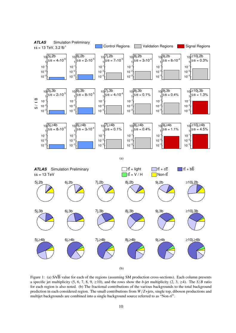
T distribution in each category. Fig-ure 2(a) compares the expected shape of the jet multiplicity distribution after preselection (described inSect. 3) between the total predicted background and several signal scenarios. Signal events have, onaverage, higher jet multiplicity than the background. Figure 2(b) compares the expected shape of the Hhad
Tdistributions between the SM four-top-quark signal and the total predicted background and also includestwo of the considered BSM signal samples. Given the different kinematic features, the Hhad
T distributionprovides a suitable discrimination between events from various signal samples and from the backgroundsamples. Comparisons between data and prediction for these distributions are shown in Sect. 7.
Number of jets
5 6 7 8 9 10 11 12 13 14 15
Arb
irta
ry u
nits
0
0.1
0.2
0.3
0.4
0.5
0.6
Total background
(SM)tttt
via CItttt
= 1 TeV)KK
2UED/RPP (m
ATLAS Simulation Preliminary
2 b≥ 5 j, ≥ = 13 TeV s
(a)
[GeV]had
TH
0 500 1000 1500 2000 2500 3000 3500 4000
Arb
irta
ry u
nits
0
0.1
0.2
0.3
0.4
0.5
0.6
Total background
(SM)tttt
via CItttt
= 1 TeV)KK
2UED/RPP (m
ATLAS Simulation Preliminary
2 b≥ 5 j, ≥ = 13 TeV s
(b)
Figure 2: Comparison of the (a) jet multiplicity and (b) HhadT distributions between some of the considered four-top-
quark signals (solid, dashed and dotted lines) and total background (shaded histogram) after the preselection. Thedistributions are normalised to unit area.
6. Systematic Uncertainties
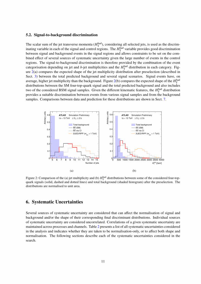
Several sources of systematic uncertainty are considered that can affect the normalisation of signal andbackground and/or the shape of their corresponding final discriminant distributions. Individual sourcesof systematic uncertainty are considered uncorrelated. Correlations of a given systematic uncertainty aremaintained across processes and channels. Table 2 presents a list of all systematic uncertainties consideredin the analysis and indicates whether they are taken to be normalisation-only, or to affect both shape andnormalisation. The following sections describe each of the systematic uncertainties considered in thesearch.
11
Systematic uncertainty Type Components
Luminosity N 1
Reconstructed objectsElectron SN 6Muon SN 9Jet energy scale SN 19Jet energy resolution SN 1b-tagging efficiency SN 6c-tagging efficiency SN 4Light-jet tagging efficiency SN 14
Background modeltt̄ cross-section N 1tt̄+HF: normalisation N 2tt̄+bb̄: NLO Shape SN 8tt̄ modelling: ISR/FSR SN 3tt̄ modelling: generator SN 3tt̄ modelling: parton shower/hadronisation SN 3W+jets normalisation N 4Z+jets normalisation N 4Single top cross-section N 1Diboson normalisation N 1tt̄V cross-section N 1tt̄H cross-section N 1Multijet normalisation N 9
Table 2: List of systematic uncertainties considered. An “N" means that the uncertainty is taken as normalisation-only for all processes and channels affected, whereas “SN" means that the uncertainty is taken to affect both shapeand normalisation. Some of the systematic uncertainties are split into several components for a more accuratetreatment.
6.1. Luminosity
The systematic uncertainty on the integrated luminosity is ±5.0%. It is derived, following a methodologysimilar to that detailed in Ref. [48], from a calibration of the luminosity scale using a pair of x − y
beam-separation scans performed in August 2015. This systematic uncertainty is applied to all processesmodelled using Monte Carlo simulations.
6.2. Uncertainties on reconstructed objects
Uncertainties associated with leptons arise from the trigger, reconstruction, identification, and isolationefficiencies, as well as the lepton momentum scale and resolution, and are studied using the Z → e+e−
and Z → µ+µ− decays in data and simulation at√
s = 13 TeV [35, 101]. In total, uncertainties associatedwith electrons (muons) include six (nine) components.
Uncertainties associated with jets primarily arise from the jet energy scale (JES) and resolution. The JESand its uncertainty are derived by combining information from test-beam data, LHC collision data andsimulation [41]. The jet energy scale uncertainty is split into 19 uncorrelated sources which have different
12
jet pT and η dependencies. Additional uncertainties are assessed in the extrapolation of the jet energyresolution from Run 1 to Run 2 conditions [41].
The efficiency of the flavour tagging algorithm is measured for each jet flavour using control samples indata and in simulation. From these measurements, correction factors are defined to correct the taggingrates in the simulation [46, 102, 103]. Uncertainties on these scale factors include a total of six independentsources affecting b-jets and four independent sources affecting c-jets. Each of these uncertainties has adifferent jet pT dependence. Fourteen uncertainties are considered for the light-jet tagging, which dependon the jet pT and η. These systematic uncertainties are taken as uncorrelated between b-jets, c-jets,and light-flavour jets. An additional uncertainty is included due to the extrapolation of the b-, c-, andlight-jet-tagging scale factors for jets with pT beyond the kinematic reach of the data calibration samplesused: pT > 300 GeV for b- and c-jets, and pT > 750 GeV for light-flavour jets.
6.3. Uncertainties on background modelling
A number of systematic uncertainties affecting the modelling of tt̄+jets are considered. These includethe uncertainty on the theoretical prediction for the inclusive cross-section, uncertainties on the overallnormalisation of the tt̄ + bb̄ and tt̄ + cc̄ background components, uncertainties associated with the choiceof matrix element generator, with the modelling of extra radiation, and with the choice of parton showerand hadronisation model, as well as additional uncertainties affecting specifically the modelling of tt̄ + bb̄production. A summary of these uncertainties is presented below.
An uncertainty of +5.5−6.1% is assigned for the inclusive tt̄ production cross-section [74–79], including
contributions from varying the factorisation and renormalisation scales and uncertainties arising from thePDF, αS and the top quark mass.
Comparisons of tt̄ + bb̄ between Powheg-Box v2 + Pythia-6.428 and a NLO prediction based on Sherpa+ OpenLoops within the acceptance of the search show that the cross-sections agree to better than 50%,which is taken as a normalisation uncertainty for tt̄ + bb̄. An overall normalisation uncertainty of 50%is assigned to the tt̄ + cc̄ component as well, taken as uncorrelated with the normalisation uncertaintyapplied to tt̄ + bb̄.
Uncertainties associated with the modelling of ISR/FSR are obtained by comparing two alternative tt̄samples generated with Powheg-Box v2 + Pythia-6.428 with settings resulting in an increased anddecreased amount of radiation compared to the nominal Powheg-Box v2 + Pythia-6.428 sample. Anuncertainty associated with the choice of the NLO generator is derived by comparing two samples, onegenerated with Powheg-Box v2 + Herwig++ and another generated with Madgraph5_aMC@NLO andinterfaced to Herwig++, and propagating the resulting fractional difference to the nominal Powheg-Box v2 + Pythia-6.428 prediction. Finally, an uncertainty due to the choice of parton shower andhadronisation model is derived by comparing events produced by Powheg-Box v2 interfaced to Pythia-6.428 or Herwig++. These three uncertainties are taken as uncorrelated between the tt̄+light, tt̄ + cc̄ andtt̄ + bb̄ processes.
Additional uncertainties affecting themodelling of tt̄+bb̄production include shape uncertainties (includinginter-category migration effects) associated with the NLO prediction from Sherpa + OpenLoops, whichis used to reweight the nominal Powheg-Box v2 + Pythia-6.428 tt̄ + bb̄ prediction. These include threedifferent scale variations, a different shower-recoil model scheme, two alternative PDF sets (MSTW andNNPDF), and a different underling event tune. Additional uncertainties for the contributions to the tt̄ + bb̄
13
background originating from MPI or FSR from top decay products and which are not part of the NLOprediction, are assessed via the alternative radiation samples. Such uncertainties cannot be applied tott̄ + cc̄, since a similar treatment of corrections and systematic uncertainties at NLO is not possible due toa lack of such a calculation. Therefore, uncertainties associated with the modelling of tt̄ + cc̄ are obtainedthrough the comparison of alternative MC samples, as mentioned above.
Uncertainties affecting the modelling of the W/Z+jets background include 5% from their respectivenormalisations to the theoretical NNLO cross-sections [104], as well as an additional 24% normalisationuncertainty added in quadrature for each additional inclusive jet-multiplicity bin beyond the one wherethe background is normalised, based on a comparison among different algorithms for merging LO matrixelements and parton showers [105]. The above uncertainties are taken as uncorrelated between W+jetsand Z+jets.
Uncertainties affecting the modelling of the single-top-quark background include a +5−4% uncertainty on
the total cross-section estimated as a weighted average of the theoretical uncertainties on t-, Wt- and s-channel production [89–91]. Uncertainties on the diboson background normalisation include 5% from theNLO theoretical cross-sections [106]. Similarly to the case of W/Z+jets an additional 24% normalisationuncertainty is added in quadrature for each additional inclusive jet multiplicity bin. Uncertainties on thett̄ +V and tt̄ +H normalisations are 15% and +10
−13% respectively, from the uncertainties on their respectiveNLO theoretical cross-sections [92, 93, 107, 108].
Uncertainties on the data-driven multijet background estimate include contributions from the limitedsample size in data, particularly at high jet and b-tag multiplicities, from the uncertainty on the real andfake efficiencies extracted from data in dedicated control regions, as well as from the extrapolation fromthese control regions to the analysis regions, as detailed in Ref. [100]. While the first source of uncertainty(the multijet statistical uncertainty) is treated together with that due to the limited amount of simulationevents (the MC statistical uncertainty), the other sources are assessed through a 50% normalisationuncertainty uncorrelated between each jet and b-tagged jet multiplicity. No explicit shape uncertainty isassigned since the large statistical uncertainties associated with the multijet background prediction, whichare uncorrelated bin-to-bin in the final discriminating variable, effectively cover shape uncertainties.
7. Results
Following the statistical method presented below, four-top-quark production signals are searched for byperforming a binned profile likelihood fit to the Hhad
T distribution simultaneously in the six control regionsand the three signal regions, excluding the nine validation regions, using a total of nine analysis topologies(described in Sect. 5.1).
7.1. Statistical interpretation
The statistical interpretation is based on a binned likelihood function L(µ, θ) constructed as a product ofPoisson probability terms over all bins considered in the search. The likelihood function depends on thesignal-strength parameter µ, amultiplicative factor to the theoretical signal production cross-section, and θ,a set of nuisance parameters that encode the effect of systematic uncertainties on the signal and backgroundexpectations and are implemented in the likelihood function as Gaussian or log-normal constraints. Thenuisance parameters θ allow variations of the expectations for signal and background according to the
14
corresponding systematic uncertainties, and their fitted values correspond to the deviations from thenominal expectations that globally provide the best fit to the data. This procedure allows a reduction of theimpact of systematic uncertainties on the search sensitivity by taking advantage of the highly populatedbackground-dominated channels included in the likelihood fit. The test statistic qµ is defined as the profilelikelihood ratio: qµ = −2 ln(L(µ, ˆ̂θµ)/L( µ̂, θ̂)), where µ̂ and θ̂ are the values of the parameters thatmaximise the likelihood function (with the constraint 0 ≤ µ̂ ≤ µ), and ˆ̂θµ are the values of the nuisanceparameters that maximise the likelihood function for a given value of µ. Uncertainties in each bin of thepredicted Hhad
T distributions due to the finite statistics of the simulated samples are also taken into accountby dedicated parameters in the fit. The test statistic qµ is implemented in the RooFit package [109, 110].In the absence of any significant excess above the background expectation, upper limits on the signalproduction cross-section for each of the signal scenarios considered in Sect. 4.1 are derived by usingqµ in the CLs method [111, 112]. For a given signal scenario, values of the production cross-section(parametrised by µ) yielding CLs< 0.05, where CLs is computed using the asymptotic approximation [113,114], are excluded at ≥95% CL.
7.2. Comparison between data and prediction prior to the fit to data
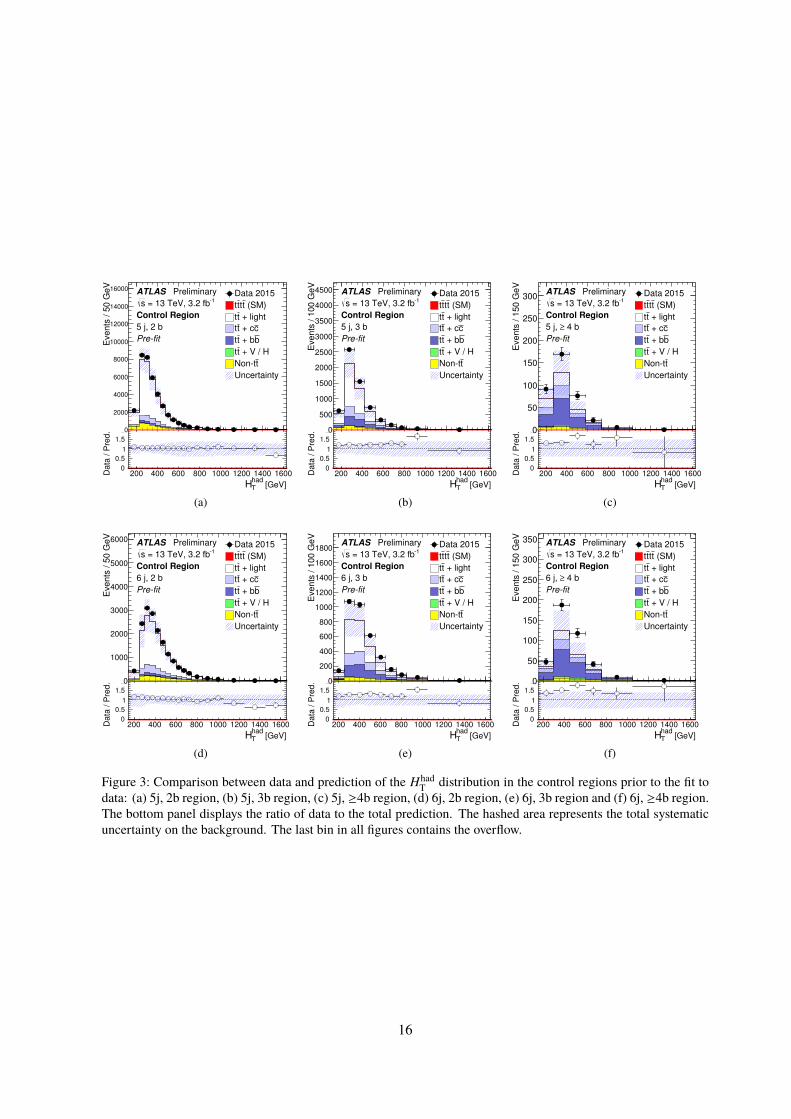
Figure 3 presents the comparison between data and prediction of the HhadT distribution in the control
regions with exactly 5 and exactly 6 jets. Figure 4 shows the comparison between data and predictionof the Hhad
T distribution in the validation regions with exactly 7, 8, 9 and ≥10 jets. The prediction ofthe Hhad
T distribution in the signal regions is given in Figure 5. A comparison of the distribution ofexpected yields per channel before the fit can be found in Figure 6(a) in the case of the control regionsand signal regions and in Figure 6(b) in the case of the validation regions. Although a normalisationdiscrepancy in the regions with large tt̄+HF contribution is observed, data agree with the SM expectationwithin the uncertainties of 10% − 50%, which are listed in Section 6. The corresponding predicted andobserved event yields for the different search channels considered are summarised in Table 3. An eventdisplay of the reconstructed event with the highest Hhad
T found in the signal region data sample is shownin Appendix A.
15
[GeV]hadTH
200 400 600 800 1000 1200 1400 1600Da
ta /
Pre
d.
0
0.5
1
1.5
2
Eve
nts
/ 5
0 G
eV
0
2000
4000
6000
8000
10000
12000
14000
16000ATLAS Preliminary
1 = 13 TeV, 3.2 fbs
Control Region
5 j, 2 b
Prefit
Data 2015
(SM)tttt
+ lighttt
c + ctt
b + btt
+ V / Htt
tNont
Uncertainty
(a) [GeV]
hadTH
200 400 600 800 1000 1200 1400 1600Da
ta /
Pre
d.
0
0.5
1
1.5
2
Eve
nts
/ 1
00 G
eV
0
500
1000
1500
2000
2500
3000
3500
4000
4500 ATLAS Preliminary1 = 13 TeV, 3.2 fbs
Control Region
5 j, 3 b
Prefit
Data 2015
(SM)tttt
+ lighttt
c + ctt
b + btt
+ V / Htt
tNont
Uncertainty
(b) [GeV]
hadTH
200 400 600 800 1000 1200 1400 1600Da
ta /
Pre
d.
0
0.5
1
1.5
2
Eve
nts
/ 1
50 G
eV
0
50
100
150
200
250
300ATLAS Preliminary
1 = 13 TeV, 3.2 fbs
Control Region
4 b≥5 j,
Prefit
Data 2015
(SM)tttt
+ lighttt
c + ctt
b + btt
+ V / Htt
tNont
Uncertainty
(c)
[GeV]hadTH
200 400 600 800 1000 1200 1400 1600Da
ta /
Pre
d.
0
0.5
1
1.5
2
Events
/ 5
0 G
eV
0
1000
2000
3000
4000
5000
6000ATLAS Preliminary
1 = 13 TeV, 3.2 fbs
Control Region
6 j, 2 b
Prefit
Data 2015
(SM)tttt
+ lighttt
c + ctt
b + btt
+ V / Htt
tNont
Uncertainty
(d) [GeV]
hadTH
200 400 600 800 1000 1200 1400 1600Da
ta /
Pre
d.
0
0.5
1
1.5
2
Eve
nts
/ 1
00 G
eV
0
200
400
600
800
1000
1200
1400
1600
1800ATLAS Preliminary
1 = 13 TeV, 3.2 fbs
Control Region
6 j, 3 b
Prefit
Data 2015
(SM)tttt
+ lighttt
c + ctt
b + btt
+ V / Htt
tNont
Uncertainty
(e) [GeV]
hadTH
200 400 600 800 1000 1200 1400 1600Da
ta /
Pre
d.
0
0.5
1
1.5
2
Eve
nts
/ 1
50 G
eV
0
50
100
150
200
250
300
350 ATLAS Preliminary1 = 13 TeV, 3.2 fbs
Control Region
4 b≥6 j,
Prefit
Data 2015
(SM)tttt
+ lighttt
c + ctt
b + btt
+ V / Htt
tNont
Uncertainty
(f)
Figure 3: Comparison between data and prediction of the HhadT distribution in the control regions prior to the fit to
data: (a) 5j, 2b region, (b) 5j, 3b region, (c) 5j, ≥4b region, (d) 6j, 2b region, (e) 6j, 3b region and (f) 6j, ≥4b region.The bottom panel displays the ratio of data to the total prediction. The hashed area represents the total systematicuncertainty on the background. The last bin in all figures contains the overflow.
16
[GeV]hadTH
200 400 600 800 1000 1200 1400 1600Da
ta /
Pre
d.
0
0.5
1
1.5
2
Eve
nts
/ 5
0 G
eV
0
200
400
600
800
1000
1200
1400
1600
1800 ATLAS Preliminary1 = 13 TeV, 3.2 fbs
Validation Region
7 j, 2 b
Prefit
Data 2015
(SM)tttt
+ lighttt
c + ctt
b + btt
+ V / Htt
tNont
Uncertainty
(a) [GeV]
hadTH
200 400 600 800 1000 1200 1400 1600Da
ta /
Pre
d.
0
0.5
1
1.5
2
Eve
nts
/ 1
00 G
eV
0
100
200
300
400
500
600
700ATLAS Preliminary
1 = 13 TeV, 3.2 fbs
Validation Region
7 j, 3 b
Prefit
Data 2015
(SM)tttt
+ lighttt
c + ctt
b + btt
+ V / Htt
tNont
Uncertainty
(b) [GeV]
hadTH
200 400 600 800 1000 1200 1400 1600Da
ta /
Pre
d.
0
0.5
1
1.5
2
Eve
nts
/ 1
50 G
eV
0
20
40
60
80
100
120
140
160
180ATLAS Preliminary
1 = 13 TeV, 3.2 fbs
Validation Region
4 b≥7 j,
Prefit
Data 2015
(SM)tttt
+ lighttt
c + ctt
b + btt
+ V / Htt
tNont
Uncertainty
(c)
[GeV]hadTH
200 400 600 800 1000 1200 1400 1600Da
ta /
Pre
d.
0
0.5
1
1.5
2
Eve
nts
/ 1
50 G
eV
0
200
400
600
800
1000
1200
1400 ATLAS Preliminary1 = 13 TeV, 3.2 fbs
Validation Region
8 j, 2 b
Prefit
Data 2015
(SM)tttt
+ lighttt
c + ctt
b + btt
+ V / Htt
tNont
Uncertainty
(d) [GeV]
hadTH
200 400 600 800 1000 1200 1400 1600Da
ta /
Pre
d.
0
0.5
1
1.5
2
Eve
nts
/ 1
50 G
eV
0
50
100
150
200
250
300
350ATLAS Preliminary
1 = 13 TeV, 3.2 fbs
Validation Region
8 j, 3 b
Prefit
Data 2015
(SM)tttt
+ lighttt
c + ctt
b + btt
+ V / Htt
tNont
Uncertainty
(e) [GeV]
hadTH
200 400 600 800 1000 1200 1400 1600Da
ta /
Pre
d.
0
0.5
1
1.5
2
Eve
nts
/ 1
50 G
eV
0
10
20
30
40
50
60
70
80
90ATLAS Preliminary
1 = 13 TeV, 3.2 fbs
Validation Region
4 b≥8 j,
Prefit
Data 2015
(SM)tttt
+ lighttt
c + ctt
b + btt
+ V / Htt
tNont
Uncertainty
(f)
[GeV]hadTH
400 600 800 1000 1200 1400 1600Da
ta /
Pre
d.
0
0.5
1
1.5
2
Eve
nts
/ 1
50 G
eV
0
50
100
150
200
250
300
350
400 ATLAS Preliminary1 = 13 TeV, 3.2 fbs
Validation Region
9 j, 2 b
Prefit
Data 2015
(SM)tttt
+ lighttt
c + ctt
b + btt
+ V / Htt
tNont
Uncertainty
(g) [GeV]
hadTH
400 600 800 1000 1200 1400 1600Da
ta /
Pre
d.
0
0.5
1
1.5
2
Eve
nts
/ 1
50 G
eV
0
20
40
60
80
100
120 ATLAS Preliminary1 = 13 TeV, 3.2 fbs
Validation Region
9 j, 3 b
Prefit
Data 2015
(SM)tttt
+ lighttt
c + ctt
b + btt
+ V / Htt
tNont
Uncertainty
(h) [GeV]
hadTH
400 600 800 1000 1200 1400 1600Da
ta /
Pre
d.
0
0.5
1
1.5
2
Eve
nts
/ 1
50 G
eV
0
20
40
60
80
100
120ATLAS Preliminary
1 = 13 TeV, 3.2 fbs
Validation Region
10 j, 2 b≥
Prefit
Data 2015
(SM)tttt
+ lighttt
c + ctt
b + btt
+ V / Htt
tNont
Uncertainty
(i)
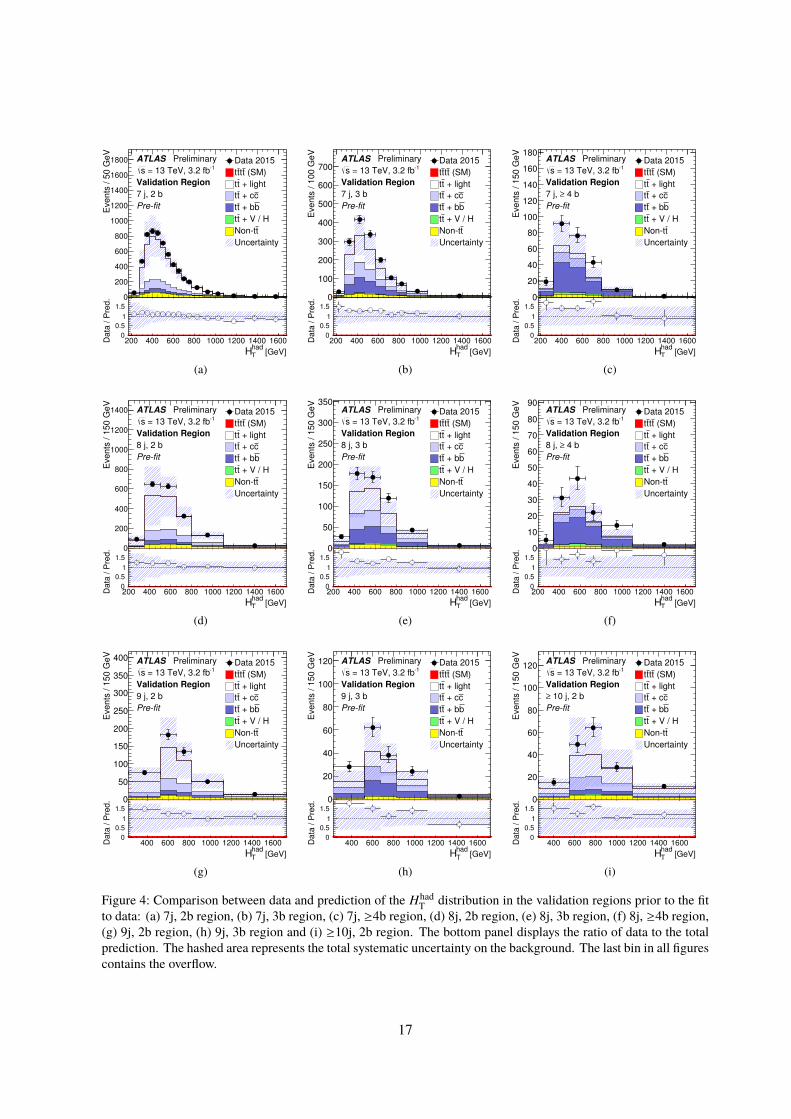
Figure 4: Comparison between data and prediction of the HhadT distribution in the validation regions prior to the fit
to data: (a) 7j, 2b region, (b) 7j, 3b region, (c) 7j, ≥4b region, (d) 8j, 2b region, (e) 8j, 3b region, (f) 8j, ≥4b region,(g) 9j, 2b region, (h) 9j, 3b region and (i) ≥10j, 2b region. The bottom panel displays the ratio of data to the totalprediction. The hashed area represents the total systematic uncertainty on the background. The last bin in all figurescontains the overflow.
17
[GeV]hadTH
400 600 800 1000 1200 1400 1600Da
ta /
Pre
d.
0
0.5
1
1.5
2
Eve
nts
/ 1
50 G
eV
0
5
10
15
20
25
30
35
40ATLAS Preliminary
1 = 13 TeV, 3.2 fbs
Signal Region
10 j, 3 b≥
Prefit
Data 2015
(SM)tttt
+ lighttt
c + ctt
b + btt
+ V / Htt
tNont
Uncertainty
(a) [GeV]
hadTH
400 600 800 1000 1200 1400 1600Da
ta /
Pre
d.
0
0.5
1
1.5
2
Eve
nts
/ 1
50 G
eV
0
5
10
15
20
25
30
35
40 ATLAS Preliminary1 = 13 TeV, 3.2 fbs
Signal Region
4 b≥9 j,
Prefit
Data 2015
(SM)tttt
+ lighttt
c + ctt
b + btt
+ V / Htt
tNont
Uncertainty
(b) [GeV]
hadTH
400 600 800 1000 1200 1400 1600Da
ta /
Pre
d.
0
0.5
1
1.5
2
Eve
nts
/ 1
50 G
eV
0
2
4
6
8
10
12
14
16 ATLAS Preliminary1 = 13 TeV, 3.2 fbs
Signal Region
4 b≥ 10 j, ≥
Prefit
Data 2015
(SM)tttt
+ lighttt
c + ctt
b + btt
+ V / Htt
tNont
Uncertainty
(c)
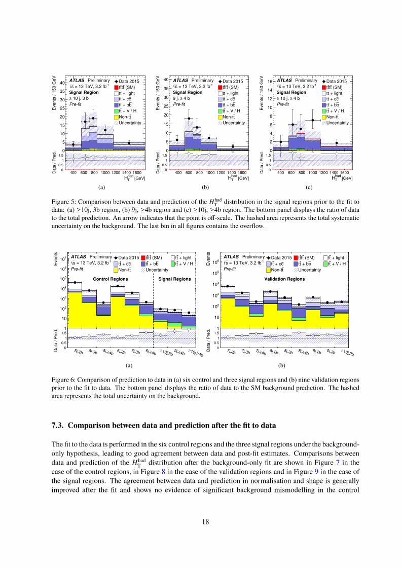
Figure 5: Comparison between data and prediction of the HhadT distribution in the signal regions prior to the fit to
data: (a) ≥10j, 3b region, (b) 9j, ≥4b region and (c) ≥10j, ≥4b region. The bottom panel displays the ratio of datato the total prediction. An arrow indicates that the point is off-scale. The hashed area represents the total systematicuncertainty on the background. The last bin in all figures contains the overflow.
5j,2b5j,3b 4b≥
5j, 6j,2b6j,3b 4b≥
6j, 10j,3b≥
4b≥9j,
4b≥10j,
≥Data
/ P
red.
0
0.5
1
1.5
2
Events
1
10
210
310
410
510
610
710ATLAS Preliminary
1 = 13 TeV, 3.2 fbs
Prefit
Data 2015 (SM)tttt + lighttt
c + ctt b + btt + V / Htt
tNont Uncertainty
Control Regions Signal Regions
(a)
7j,2b7j,3b 4b≥
7j, 8j,2b8j,3b 4b≥
8j, 9j,2b9j,3b 10j,2b
≥Data
/ P
red.
0
0.5
1
1.5
2
Events
1
10
210
310
410
510
610
ATLAS Preliminary1 = 13 TeV, 3.2 fbs
Prefit
Data 2015 (SM)tttt + lighttt
c + ctt b + btt + V / Htt
tNont Uncertainty
Validation Regions
(b)
Figure 6: Comparison of prediction to data in (a) six control and three signal regions and (b) nine validation regionsprior to the fit to data. The bottom panel displays the ratio of data to the SM background prediction. The hashedarea represents the total uncertainty on the background.
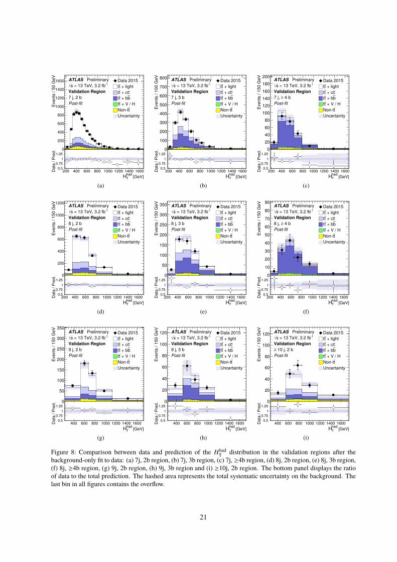
7.3. Comparison between data and prediction after the fit to data
The fit to the data is performed in the six control regions and the three signal regions under the background-only hypothesis, leading to good agreement between data and post-fit estimates. Comparisons betweendata and prediction of the Hhad
T distribution after the background-only fit are shown in Figure 7 in thecase of the control regions, in Figure 8 in the case of the validation regions and in Figure 9 in the case ofthe signal regions. The agreement between data and prediction in normalisation and shape is generallyimproved after the fit and shows no evidence of significant background mismodelling in the control
18
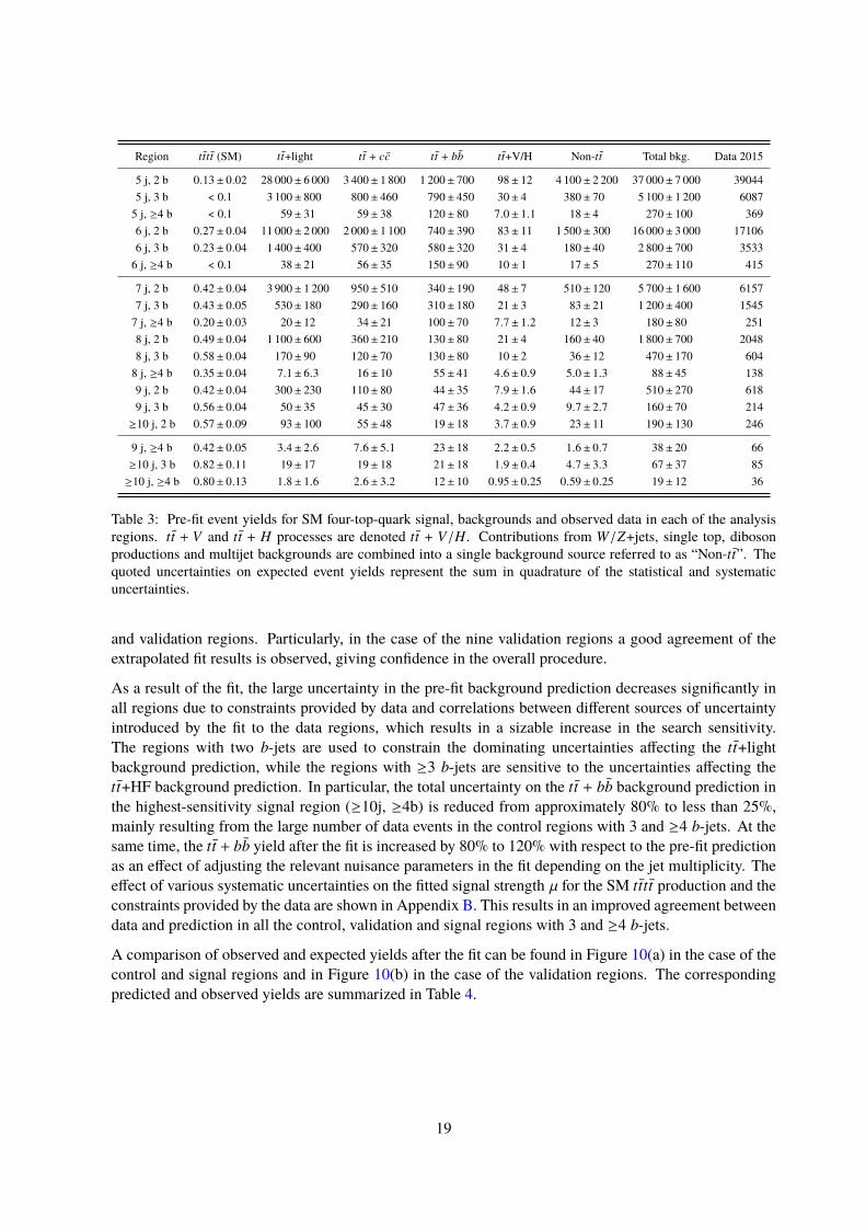
Region tt̄tt̄ (SM) tt̄+light tt̄ + cc̄ tt̄ + bb̄ tt̄+V/H Non-tt̄ Total bkg. Data 2015
5 j, 2 b 0.13± 0.02 28 000± 6 000 3 400± 1 800 1 200± 700 98± 12 4 100± 2 200 37 000± 7 000 390445 j, 3 b < 0.1 3 100± 800 800± 460 790± 450 30± 4 380± 70 5 100± 1 200 60875 j, ≥4 b < 0.1 59± 31 59± 38 120± 80 7.0± 1.1 18± 4 270± 100 3696 j, 2 b 0.27± 0.04 11 000± 2 000 2 000± 1 100 740± 390 83± 11 1 500± 300 16 000± 3 000 171066 j, 3 b 0.23± 0.04 1 400± 400 570± 320 580± 320 31± 4 180± 40 2 800± 700 35336 j, ≥4 b < 0.1 38± 21 56± 35 150± 90 10± 1 17± 5 270± 110 415
7 j, 2 b 0.42± 0.04 3 900± 1 200 950± 510 340± 190 48± 7 510± 120 5 700± 1 600 61577 j, 3 b 0.43± 0.05 530± 180 290± 160 310± 180 21± 3 83± 21 1 200± 400 15457 j, ≥4 b 0.20± 0.03 20± 12 34± 21 100± 70 7.7± 1.2 12± 3 180± 80 2518 j, 2 b 0.49± 0.04 1 100± 600 360± 210 130± 80 21± 4 160± 40 1 800± 700 20488 j, 3 b 0.58± 0.04 170± 90 120± 70 130± 80 10± 2 36± 12 470± 170 6048 j, ≥4 b 0.35± 0.04 7.1± 6.3 16± 10 55± 41 4.6± 0.9 5.0± 1.3 88± 45 1389 j, 2 b 0.42± 0.04 300± 230 110± 80 44± 35 7.9± 1.6 44± 17 510± 270 6189 j, 3 b 0.56± 0.04 50± 35 45± 30 47± 36 4.2± 0.9 9.7± 2.7 160± 70 214≥10 j, 2 b 0.57± 0.09 93± 100 55± 48 19± 18 3.7± 0.9 23± 11 190± 130 246
9 j, ≥4 b 0.42± 0.05 3.4± 2.6 7.6± 5.1 23± 18 2.2± 0.5 1.6± 0.7 38± 20 66≥10 j, 3 b 0.82± 0.11 19± 17 19± 18 21± 18 1.9± 0.4 4.7± 3.3 67± 37 85≥10 j, ≥4 b 0.80± 0.13 1.8± 1.6 2.6± 3.2 12± 10 0.95± 0.25 0.59± 0.25 19± 12 36
Table 3: Pre-fit event yields for SM four-top-quark signal, backgrounds and observed data in each of the analysisregions. tt̄ + V and tt̄ + H processes are denoted tt̄ + V/H . Contributions from W/Z+jets, single top, dibosonproductions and multijet backgrounds are combined into a single background source referred to as “Non-tt̄”. Thequoted uncertainties on expected event yields represent the sum in quadrature of the statistical and systematicuncertainties.
and validation regions. Particularly, in the case of the nine validation regions a good agreement of theextrapolated fit results is observed, giving confidence in the overall procedure.
As a result of the fit, the large uncertainty in the pre-fit background prediction decreases significantly inall regions due to constraints provided by data and correlations between different sources of uncertaintyintroduced by the fit to the data regions, which results in a sizable increase in the search sensitivity.The regions with two b-jets are used to constrain the dominating uncertainties affecting the tt̄+lightbackground prediction, while the regions with ≥3 b-jets are sensitive to the uncertainties affecting thett̄+HF background prediction. In particular, the total uncertainty on the tt̄ + bb̄ background prediction inthe highest-sensitivity signal region (≥10j, ≥4b) is reduced from approximately 80% to less than 25%,mainly resulting from the large number of data events in the control regions with 3 and ≥4 b-jets. At thesame time, the tt̄ + bb̄ yield after the fit is increased by 80% to 120% with respect to the pre-fit predictionas an effect of adjusting the relevant nuisance parameters in the fit depending on the jet multiplicity. Theeffect of various systematic uncertainties on the fitted signal strength µ for the SM tt̄tt̄ production and theconstraints provided by the data are shown in Appendix B. This results in an improved agreement betweendata and prediction in all the control, validation and signal regions with 3 and ≥4 b-jets.
A comparison of observed and expected yields after the fit can be found in Figure 10(a) in the case of thecontrol and signal regions and in Figure 10(b) in the case of the validation regions. The correspondingpredicted and observed yields are summarized in Table 4.
19
[GeV]hadTH
200 400 600 800 1000 1200 1400 1600Da
ta /
Pre
d.
0.5
0.75
1
1.25
1.5
Eve
nts
/ 5
0 G
eV
0
2000
4000
6000
8000
10000
12000
14000ATLAS Preliminary
1 = 13 TeV, 3.2 fbs
Control Region
5 j, 2 b
Postfit
Data 2015
+ lighttt
c + ctt
b + btt
+ V / Htt
tNont
Uncertainty
(a) [GeV]
hadTH
200 400 600 800 1000 1200 1400 1600Da
ta /
Pre
d.
0.5
0.75
1
1.25
1.5
Eve
nts
/ 1
00 G
eV
0
500
1000
1500
2000
2500
3000
3500
4000
4500 ATLAS Preliminary1 = 13 TeV, 3.2 fbs
Control Region
5 j, 3 b
Postfit
Data 2015
+ lighttt
c + ctt
b + btt
+ V / Htt
tNont
Uncertainty
(b) [GeV]
hadTH
200 400 600 800 1000 1200 1400 1600Da
ta /
Pre
d.
0.5
0.75
1
1.25
1.5
Eve
nts
/ 1
50 G
eV
0
50
100
150
200
250
300
ATLAS Preliminary1 = 13 TeV, 3.2 fbs
Control Region
4 b≥5 j,
Postfit
Data 2015
+ lighttt
c + ctt
b + btt
+ V / Htt
tNont
Uncertainty
(c)
[GeV]hadTH
200 400 600 800 1000 1200 1400 1600Da
ta /
Pre
d.
0.5
0.75
1
1.25
1.5
Events
/ 5
0 G
eV
0
1000
2000
3000
4000
5000
ATLAS Preliminary1 = 13 TeV, 3.2 fbs
Control Region
6 j, 2 b
Postfit
Data 2015
+ lighttt
c + ctt
b + btt
+ V / Htt
tNont
Uncertainty
(d) [GeV]
hadTH
200 400 600 800 1000 1200 1400 1600Da
ta /
Pre
d.
0.5
0.75
1
1.25
1.5
Eve
nts
/ 1
00 G
eV
0
200
400
600
800
1000
1200
1400
1600
1800ATLAS Preliminary
1 = 13 TeV, 3.2 fbs
Control Region
6 j, 3 b
Postfit
Data 2015
+ lighttt
c + ctt
b + btt
+ V / Htt
tNont
Uncertainty
(e) [GeV]
hadTH
200 400 600 800 1000 1200 1400 1600Da
ta /
Pre
d.
0.5
0.75
1
1.25
1.5
Eve
nts
/ 1
50 G
eV
0
50
100
150
200
250
300
350 ATLAS Preliminary1 = 13 TeV, 3.2 fbs
Control Region
4 b≥6 j,
Postfit
Data 2015
+ lighttt
c + ctt
b + btt
+ V / Htt
tNont
Uncertainty
(f)
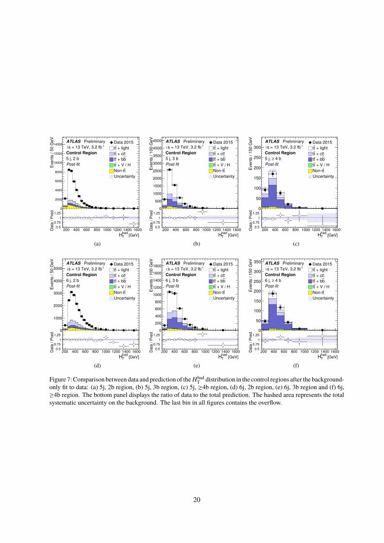
Figure 7:Comparison between data and prediction of the HhadT distribution in the control regions after the background-
only fit to data: (a) 5j, 2b region, (b) 5j, 3b region, (c) 5j, ≥4b region, (d) 6j, 2b region, (e) 6j, 3b region and (f) 6j,≥4b region. The bottom panel displays the ratio of data to the total prediction. The hashed area represents the totalsystematic uncertainty on the background. The last bin in all figures contains the overflow.
20
[GeV]hadTH
200 400 600 800 1000 1200 1400 1600Da
ta /
Pre
d.
0.5
0.75
1
1.25
1.5
Eve
nts
/ 5
0 G
eV
0
200
400
600
800
1000
1200
1400
1600 ATLAS Preliminary1 = 13 TeV, 3.2 fbs
Validation Region
7 j, 2 b
Postfit
Data 2015
+ lighttt
c + ctt
b + btt
+ V / Htt
tNont
Uncertainty
(a) [GeV]
hadTH
200 400 600 800 1000 1200 1400 1600Da
ta /
Pre
d.
0.5
0.75
1
1.25
1.5
Eve
nts
/ 1
00 G
eV
0
100
200
300
400
500
600
700
800ATLAS Preliminary
1 = 13 TeV, 3.2 fbs
Validation Region
7 j, 3 b
Postfit
Data 2015
+ lighttt
c + ctt
b + btt
+ V / Htt
tNont
Uncertainty
(b) [GeV]
hadTH
200 400 600 800 1000 1200 1400 1600Da
ta /
Pre
d.
0.5
0.75
1
1.25
1.5
Eve
nts
/ 1
50 G
eV
0
20
40
60
80
100
120
140
160
180
200ATLAS Preliminary
1 = 13 TeV, 3.2 fbs
Validation Region
4 b≥7 j,
Postfit
Data 2015
+ lighttt
c + ctt
b + btt
+ V / Htt
tNont
Uncertainty
(c)
[GeV]hadTH
200 400 600 800 1000 1200 1400 1600Da
ta /
Pre
d.
0.5
0.75
1
1.25
1.5
Eve
nts
/ 1
50 G
eV
0
200
400
600
800
1000
1200ATLAS Preliminary
1 = 13 TeV, 3.2 fbs
Validation Region
8 j, 2 b
Postfit
Data 2015
+ lighttt
c + ctt
b + btt
+ V / Htt
tNont
Uncertainty
(d) [GeV]
hadTH
200 400 600 800 1000 1200 1400 1600Da
ta /
Pre
d.
0.5
0.75
1
1.25
1.5
Eve
nts
/ 1
50 G
eV
0
50
100
150
200
250
300
350 ATLAS Preliminary1 = 13 TeV, 3.2 fbs
Validation Region
8 j, 3 b
Postfit
Data 2015
+ lighttt
c + ctt
b + btt
+ V / Htt
tNont
Uncertainty
(e) [GeV]
hadTH
200 400 600 800 1000 1200 1400 1600Da
ta /
Pre
d.
0.5
0.75
1
1.25
1.5
Eve
nts
/ 1
50 G
eV
0
10
20
30
40
50
60
70
80
90ATLAS Preliminary
1 = 13 TeV, 3.2 fbs
Validation Region
4 b≥8 j,
Postfit
Data 2015
+ lighttt
c + ctt
b + btt
+ V / Htt
tNont
Uncertainty
(f)
[GeV]hadTH
400 600 800 1000 1200 1400 1600Da
ta /
Pre
d.
0.5
0.75
1
1.25
1.5
Eve
nts
/ 1
50 G
eV
0
50
100
150
200
250
300
350ATLAS Preliminary
1 = 13 TeV, 3.2 fbs
Validation Region
9 j, 2 b
Postfit
Data 2015
+ lighttt
c + ctt
b + btt
+ V / Htt
tNont
Uncertainty
(g) [GeV]
hadTH
400 600 800 1000 1200 1400 1600Da
ta /
Pre
d.
0.5
0.75
1
1.25
1.5
Eve
nts
/ 1
50 G
eV
0
20
40
60
80
100
120 ATLAS Preliminary1 = 13 TeV, 3.2 fbs
Validation Region
9 j, 3 b
Postfit
Data 2015
+ lighttt
c + ctt
b + btt
+ V / Htt
tNont
Uncertainty
(h) [GeV]
hadTH
400 600 800 1000 1200 1400 1600Da
ta /
Pre
d.
0.5
0.75
1
1.25
1.5
Eve
nts
/ 1
50 G
eV
0
20
40
60
80
100
120ATLAS Preliminary
1 = 13 TeV, 3.2 fbs
Validation Region
10 j, 2 b≥
Postfit
Data 2015
+ lighttt
c + ctt
b + btt
+ V / Htt
tNont
Uncertainty
(i)
Figure 8: Comparison between data and prediction of the HhadT distribution in the validation regions after the
background-only fit to data: (a) 7j, 2b region, (b) 7j, 3b region, (c) 7j, ≥4b region, (d) 8j, 2b region, (e) 8j, 3b region,(f) 8j, ≥4b region, (g) 9j, 2b region, (h) 9j, 3b region and (i) ≥10j, 2b region. The bottom panel displays the ratioof data to the total prediction. The hashed area represents the total systematic uncertainty on the background. Thelast bin in all figures contains the overflow.
21
[GeV]hadTH
400 600 800 1000 1200 1400 1600Da
ta /
Pre
d.
0.5
0.75
1
1.25
1.5
Eve
nts
/ 1
50 G
eV
0
5
10
15
20
25
30
35
40ATLAS Preliminary
1 = 13 TeV, 3.2 fbs
Signal Region
10 j, 3 b≥
Postfit
Data 2015
(SM)*tttt
+ lighttt
c + ctt
b + btt
+ V / Htt
tNont
Uncertainty
*: signal normalised to total background
(a) [GeV]
hadTH
400 600 800 1000 1200 1400 1600Da
ta /
Pre
d.
0.5
0.75
1
1.25
1.5
Eve
nts
/ 1
50 G
eV
0
5
10
15
20
25
30
35
40 ATLAS Preliminary1 = 13 TeV, 3.2 fbs
Signal Region
4 b≥9 j,
Postfit
Data 2015
(SM)*tttt
+ lighttt
c + ctt
b + btt
+ V / Htt
tNont
Uncertainty
*: signal normalised to total background
(b) [GeV]
hadTH
400 600 800 1000 1200 1400 1600Da
ta /
Pre
d.
0.5
0.75
1
1.25
1.5
Eve
nts
/ 1
50 G
eV
0
2
4
6
8
10
12
14
16 ATLAS Preliminary1 = 13 TeV, 3.2 fbs
Signal Region
4 b≥ 10 j, ≥
Postfit
Data 2015
(SM)*tttt
+ lighttt
c + ctt
b + btt
+ V / Htt
tNont
Uncertainty
*: signal normalised to total background
(c)
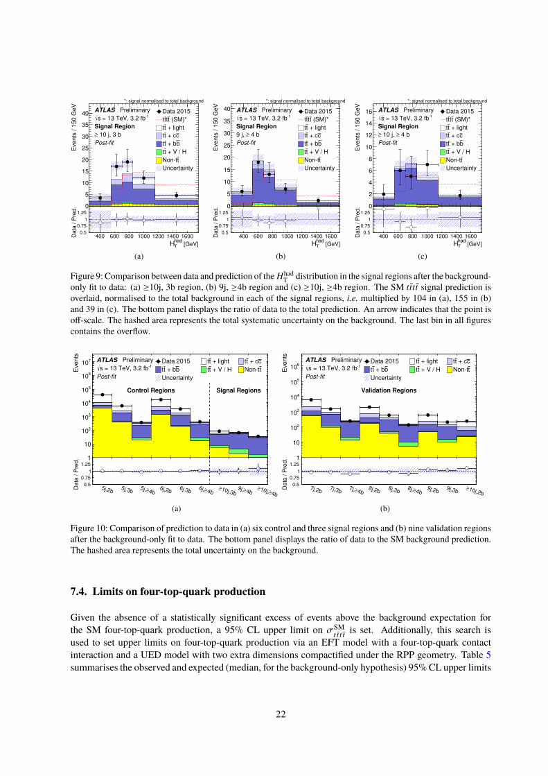
Figure 9: Comparison between data and prediction of the HhadT distribution in the signal regions after the background-
only fit to data: (a) ≥10j, 3b region, (b) 9j, ≥4b region and (c) ≥10j, ≥4b region. The SM tt̄tt̄ signal prediction isoverlaid, normalised to the total background in each of the signal regions, i.e. multiplied by 104 in (a), 155 in (b)and 39 in (c). The bottom panel displays the ratio of data to the total prediction. An arrow indicates that the point isoff-scale. The hashed area represents the total systematic uncertainty on the background. The last bin in all figurescontains the overflow.
5j,2b5j,3b 4b≥
5j, 6j,2b6j,3b 4b≥
6j, 10j,3b≥
4b≥9j,
4b≥10j,
≥Data
/ P
red.
0.5
0.75
1
1.25
1.5
Events
1
10
210
310
410
510
610
710 ATLAS Preliminary1 = 13 TeV, 3.2 fbs
Postfit
Data 2015 + lighttt c + ctt
b + btt + V / Htt tNont
Uncertainty
Control Regions Signal Regions
(a)
7j,2b7j,3b 4b≥
7j, 8j,2b8j,3b 4b≥
8j, 9j,2b9j,3b 10j,2b
≥Data
/ P
red.
0.5
0.75
1
1.25
1.5
Events
1
10
210
310
410
510
610
ATLAS Preliminary1 = 13 TeV, 3.2 fbs
Postfit
Data 2015 + lighttt c + ctt
b + btt + V / Htt tNont
Uncertainty
Validation Regions
(b)
Figure 10: Comparison of prediction to data in (a) six control and three signal regions and (b) nine validation regionsafter the background-only fit to data. The bottom panel displays the ratio of data to the SM background prediction.The hashed area represents the total uncertainty on the background.
7.4. Limits on four-top-quark production
Given the absence of a statistically significant excess of events above the background expectation forthe SM four-top-quark production, a 95% CL upper limit on σSM
t t̄t t̄is set. Additionally, this search is
used to set upper limits on four-top-quark production via an EFT model with a four-top-quark contactinteraction and a UED model with two extra dimensions compactified under the RPP geometry. Table 5summarises the observed and expected (median, for the background-only hypothesis) 95%CL upper limits
22
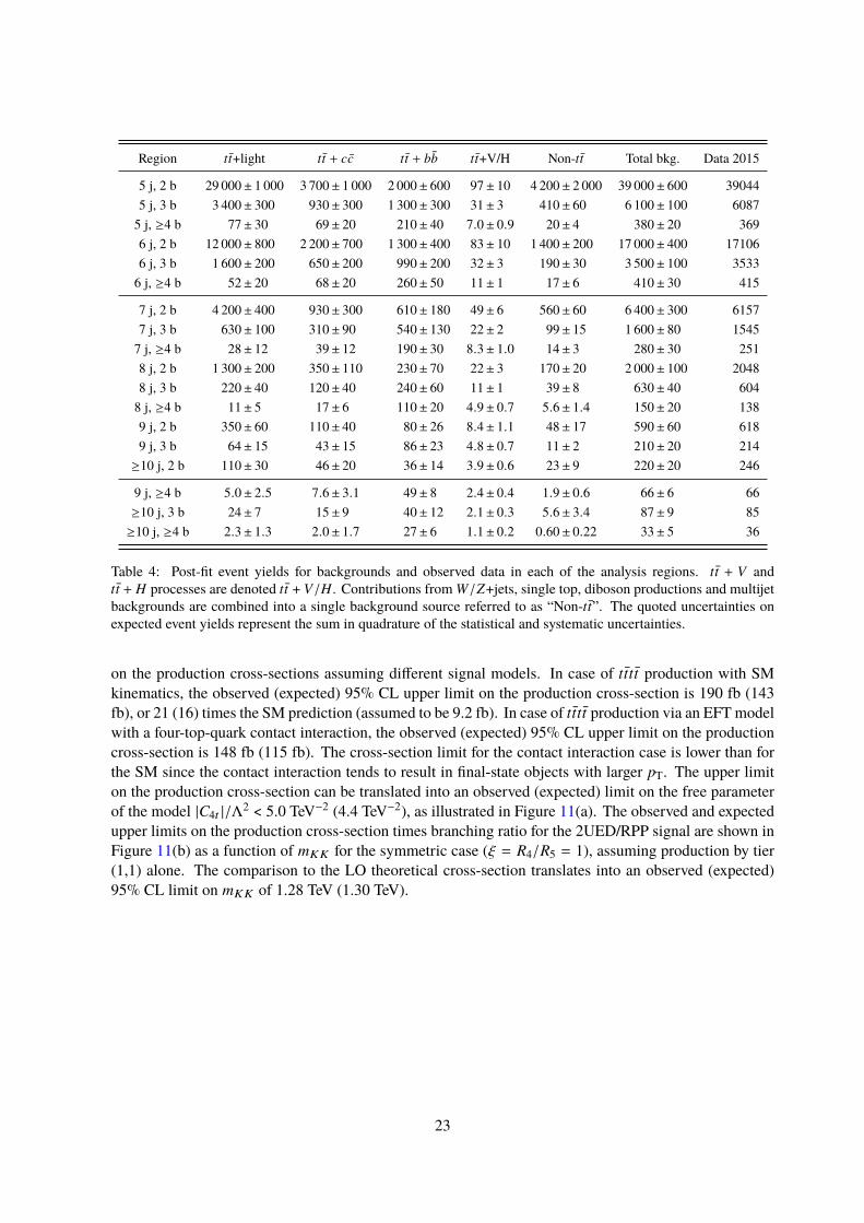
Region tt̄+light tt̄ + cc̄ tt̄ + bb̄ tt̄+V/H Non-tt̄ Total bkg. Data 2015
5 j, 2 b 29 000± 1 000 3 700± 1 000 2 000± 600 97± 10 4 200± 2 000 39 000± 600 390445 j, 3 b 3 400± 300 930± 300 1 300± 300 31± 3 410± 60 6 100± 100 60875 j, ≥4 b 77± 30 69± 20 210± 40 7.0± 0.9 20± 4 380± 20 3696 j, 2 b 12 000± 800 2 200± 700 1 300± 400 83± 10 1 400± 200 17 000± 400 171066 j, 3 b 1 600± 200 650± 200 990± 200 32± 3 190± 30 3 500± 100 35336 j, ≥4 b 52± 20 68± 20 260± 50 11± 1 17± 6 410± 30 415
7 j, 2 b 4 200± 400 930± 300 610± 180 49± 6 560± 60 6 400± 300 61577 j, 3 b 630± 100 310± 90 540± 130 22± 2 99± 15 1 600± 80 15457 j, ≥4 b 28± 12 39± 12 190± 30 8.3± 1.0 14± 3 280± 30 2518 j, 2 b 1 300± 200 350± 110 230± 70 22± 3 170± 20 2 000± 100 20488 j, 3 b 220± 40 120± 40 240± 60 11± 1 39± 8 630± 40 6048 j, ≥4 b 11± 5 17± 6 110± 20 4.9± 0.7 5.6± 1.4 150± 20 1389 j, 2 b 350± 60 110± 40 80± 26 8.4± 1.1 48± 17 590± 60 6189 j, 3 b 64± 15 43± 15 86± 23 4.8± 0.7 11± 2 210± 20 214≥10 j, 2 b 110± 30 46± 20 36± 14 3.9± 0.6 23± 9 220± 20 246
9 j, ≥4 b 5.0± 2.5 7.6± 3.1 49± 8 2.4± 0.4 1.9± 0.6 66± 6 66≥10 j, 3 b 24± 7 15± 9 40± 12 2.1± 0.3 5.6± 3.4 87± 9 85≥10 j, ≥4 b 2.3± 1.3 2.0± 1.7 27± 6 1.1± 0.2 0.60± 0.22 33± 5 36
Table 4: Post-fit event yields for backgrounds and observed data in each of the analysis regions. tt̄ + V andtt̄ + H processes are denoted tt̄ + V/H . Contributions from W/Z+jets, single top, diboson productions and multijetbackgrounds are combined into a single background source referred to as “Non-tt̄”. The quoted uncertainties onexpected event yields represent the sum in quadrature of the statistical and systematic uncertainties.
on the production cross-sections assuming different signal models. In case of tt̄tt̄ production with SMkinematics, the observed (expected) 95% CL upper limit on the production cross-section is 190 fb (143fb), or 21 (16) times the SM prediction (assumed to be 9.2 fb). In case of tt̄tt̄ production via an EFT modelwith a four-top-quark contact interaction, the observed (expected) 95% CL upper limit on the productioncross-section is 148 fb (115 fb). The cross-section limit for the contact interaction case is lower than forthe SM since the contact interaction tends to result in final-state objects with larger pT. The upper limiton the production cross-section can be translated into an observed (expected) limit on the free parameterof the model |C4t |/Λ
2 < 5.0 TeV−2 (4.4 TeV−2), as illustrated in Figure 11(a). The observed and expectedupper limits on the production cross-section times branching ratio for the 2UED/RPP signal are shown inFigure 11(b) as a function of mKK for the symmetric case (ξ = R4/R5 = 1), assuming production by tier(1,1) alone. The comparison to the LO theoretical cross-section translates into an observed (expected)95% CL limit on mKK of 1.28 TeV (1.30 TeV).
23
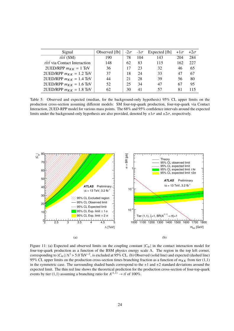
Signal Observed [fb] -2σ -1σ Expected [fb] +1σ +2σtt̄tt̄ (SM) 190 78 104 143 204 284
tt̄tt̄ via Contact Interaction 148 62 83 115 162 2272UED/RPP mKK = 1 TeV 36 17 23 32 46 652UED/RPP mKK = 1.2 TeV 37 18 24 33 47 672UED/RPP mKK = 1.4 TeV 44 21 28 39 56 802UED/RPP mKK = 1.6 TeV 52 25 34 47 67 952UED/RPP mKK = 1.8 TeV 62 30 41 57 81 115
Table 5: Observed and expected (median, for the background-only hypothesis) 95% CL upper limits on theproduction cross-section assuming different models: SM four-top-quark production, four-top-quark via ContactInteraction, 2UED-RPP model for various mass points. The 68% and 95% confidence intervals around the expectedlimits under the background-only hypothesis are also provided, denoted by ±1σ and ±2σ, respectively.
[TeV]Λ
2 2.5 3 3.5 4 4.5 5
|4t
|C
0
10
20
30
40
50
60
70
80
95% CL Excluded region
95% CL Observed limit
95% CL Expected limit
σ 1 ±95% CL Exp. limit
σ 2 ±95% CL Exp. limit
ATLAS Preliminary1 = 13 TeV, 3.2 fbs
(a)
[GeV]KKm
1000 1100 1200 1300 1400 1500 1600 1700 1800
BR
[pb]
× σ
2−10
1−10
1
Theory95% CL observed limit95% CL expected limit
σ1±95% CL expected limit σ2±95% CL expected limit
ATLAS Preliminary
1 = 13 TeV, 3.2 fbs
)=1t t→(1,1)
=1, BR(AξTier (1,1),
(b)
Figure 11: (a) Expected and observed limits on the coupling constant |C4t | in the contact interaction model forfour-top-quark production as a function of the BSM physics energy scale Λ. The region in the top left corner,corresponding to |C4t |/Λ
2 > 5.0 TeV−2, is excluded at 95% CL. (b) Observed (solid line) and expected (dashed line)95% CL upper limits on the production cross-section times branching fraction as a function of mKK from tier (1,1)in the symmetric case. The surrounding shaded bands correspond to the ±1 and ±2 standard deviations around theexpected limit. The thin red line shows the theoretical prediction for the production cross-section of four-top-quarkevents by tier (1,1) assuming a branching ratio for A(1,1) → tt̄ of 100%.
24
8. Summary
A search for four-top-quark production in the resolved single-lepton channel, characterised by an isolatedelectron or muon with high transverse momentum and a large number of jets, has been presented. Theanalysed data sample consists of 3.2 fb−1 of proton-proton collisions at
√s = 13 TeV collected with
the ATLAS detector at the Large Hadron Collider during 2015. In order to improve the sensitivity ofthe search, events are categorised according to their jet and b-tagged jet multiplicities. Background-dominated samples with lower jet and/or b-tagged jet multiplicities are exploited to constrain in situ thesystematic uncertainties affecting the background prediction. No significant excess of events above the SMbackground expectation is found. For the tt̄tt̄ production with SM kinematics, an observed (expected) 95%CL upper limit on the production cross-section of 190 fb (143 fb), or 21 (16) times the SM prediction, isobtained, representing the most restrictive limit to date. Additionally, upper bounds on the four-top-quarkproduction cross-section are set in several BSM scenarios, including a four-fermion contact interaction,and a universal extra dimensions model.
25
References
[1] E. Boos et al., The top quark (20 years after the discovery), Phys. Usp. 58 (2015) 1241,arXiv: 1509.03325 [hep-ex].
[2] L. Susskind, Dynamics of Spontaneous Symmetry Breaking in the Weinberg-Salam Theory,Phys. Rev. D 20 (1979) 2619.
[3] C. T. Hill and E. H. Simmons, Strong dynamics and electroweak symmetry breaking,Phys. Rept. 381 (2003) 235, arXiv: hep-ph/0203079.
[4] N. Arkani-Hamed et al., The Littlest Higgs, JHEP 0207 (2002) 034, arXiv: hep-ph/0206021.
[5] D. B. Kaplan, H. Georgi and S. Dimopoulos, Composite Higgs Scalars,Phys. Lett. B 136 (1984) 187.
[6] ATLAS Collaboration,Observation of top-quark pair production in association with a photon and measurement of thett̄γ production cross section in pp collisions at
√s = 7 TeV using the ATLAS detector,
Phys. Rev. D 91 (2015) 072007, arXiv: 1502.00586 [hep-ex].[7] ATLAS Collaboration, Measurement of the tt̄W and tt̄ Z production cross sections in pp
collisions at√
s = 8 TeV with the ATLAS detector, JHEP 1511 (2015) 172,arXiv: 1509.05276 [hep-ex].
[8] CMS Collaboration, Observation of top quark pairs produced in association with a vector bosonin pp collisions at
√s = 8 TeV, JHEP 1601 (2016) 096, arXiv: 1510.01131 [hep-ex].
[9] ATLAS Collaboration,Measurements of fiducial cross-sections for tt̄ production with one or twoadditional b-jets in pp collisions at
√s = 8 TeV using the ATLAS detector,
Eur. Phys. J. C 76 (2015) 11. 38 p, arXiv: 1508.06868 [hep-ex].[10] CMS Collaboration,
Measurement of the cross section ratio σtt̄bb̄/σtt̄jj in pp collisions at√
s = 8 TeV,Phys. Lett. B 746 (2015) 132, arXiv: 1411.5621 [hep-ex].
[11] CMS Collaboration, Measurement of tt̄ production with additional jet activity, including b quarkjets, in the dilepton decay channel using pp collisions at
√s = 8 TeV, CMS-TOP-12-041, 2015,
url: https://cds.cern.ch/record/2058475.
[12] The ATLAS and CMS Collaborations,Measurements of the Higgs boson production and decay rates and constraints on its couplingsfrom a combined ATLAS and CMS analysis of the LHC pp collision data at
√s = 7 and 8 TeV,
ATLAS-CONF-2015-044, CMS-PAS-HIG-15-002, 2015,url: https://cds.cern.ch/record/2052552.
[13] B. S. Acharya et al., Identifying Multi-Top Events from Gluino Decay at the LHC (2009),arXiv: 0901.3367 [hep-ph].
[14] A. Deandrea and N. Deutschmann, Multi-tops at the LHC, JHEP 1408 (2014) 134,arXiv: 1405.6119 [hep-ph].
[15] A. De Simone et al., A First Top Partner Hunter’s Guide, JHEP 1304 (2013) 004,arXiv: 1211.5663 [hep-ph].
[16] A. Pomarol and J. Serra, Top Quark Compositeness: Feasibility and Implications,Phys. Rev. D 78 (2008) 074026, arXiv: 0806.3247 [hep-ph].
26
[17] M. Guchait, F. Mahmoudi and K. Sridhar,Associated production of a Kaluza-Klein excitation of a gluon with a tt̄ pair at the LHC,Phys. Lett. B 666 (2008) 347, arXiv: 0710.2234 [hep-ph].
[18] T. Plehn and T. M. P. Tait, Seeking Sgluons, J. Phys. G 36 (2009) 075001,arXiv: 0810.3919 [hep-ph].
[19] C. Kilic, T. Okui and R. Sundrum, Vectorlike Confinement at the LHC, JHEP 1002 (2010) 018,arXiv: 0906.0577 [hep-ph].
[20] G. Cacciapaglia et al., Four tops on the real projective plane at LHC, JHEP 1110 (2011) 042,arXiv: 1107.4616 [hep-ph].
[21] C. Degrande et al., Non-resonant New Physics in Top Pair Production at Hadron Colliders,JHEP 1103 (2011) 125, arXiv: 1010.6304 [hep-ph].
[22] G. Cacciapaglia, A. Deandrea and J. Llodra-Perez,A Dark Matter candidate from Lorentz Invariance in 6D, JHEP 1003 (2010) 083,arXiv: 0907.4993 [hep-ph].
[23] ATLAS Collaboration, Search for production of vector-like quark pairs and of four top quarks inthe lepton-plus-jets final state in pp collisions at
√s = 8 TeV with the ATLAS detector,
JHEP 1508 (2015) 105, arXiv: 1505.04306 [hep-ex].[24] ATLAS Collaboration, Analysis of events with b-jets and a pair of leptons of the same charge in
pp collisions at√
s = 8 TeV with the ATLAS detector, JHEP 1510 (2015) 150,arXiv: 1504.04605 [hep-ex].
[25] CMS Collaboration, Search for standard model production of four top quarks in the lepton + jetschannel in pp collisions at
√s = 8 TeV, JHEP 1411 (2014) 154, arXiv: 1409.7339 [hep-ex].
[26] CMS Collaboration,Search for new physics in events with same-sign dileptons and jets in pp collisions at
√s = 8 TeV,
JHEP 1401 (2014) 163, arXiv: 1311.6736 [hep-ex].[27] G. Bevilacqua and M. Worek, Constraining BSM Physics at the LHC: Four top final states with
NLO accuracy in perturbative QCD, JHEP 1207 (2012) 111, arXiv: 1206.3064 [hep-ph].[28] J. Alwall et al., The automated computation of tree-level and next-to-leading order differential
cross sections, and their matching to parton shower simulations, JHEP 1407 (2014) 079,arXiv: 1405.0301 [hep-ph].
[29] K. A. Olive et al., Review of Particle Physics, Chin. Phys. C 38 (2014) 090001.[30] ATLAS Collaboration, The ATLAS Experiment at the CERN Large Hadron Collider,
JINST 3 (2008) S08003.[31] M Capeans et al., ATLAS Insertable B-Layer Technical Design Report, ATLAS-TDR-19, 2010,
url: https://cds.cern.ch/record/1291633.[32] S. Artz et al., Upgrade of the ATLAS Central Trigger for LHC Run-2, JINST 10 (2015) C02030.[33] ATLAS Collaboration, Electron reconstruction and identification efficiency measurements with
the ATLAS detector using the 2011 LHC proton-proton collision data,Eur. Phys. J. C 74 (2014) 2941, arXiv: 1404.2240 [hep-ex].
[34] ATLAS Collaboration,Electron and photon energy calibration with the ATLAS detector using LHC Run 1 data,Eur. Phys. J. C 74 (2014) 3071, arXiv: 1407.5063 [hep-ex].
27
[35] ATLAS Collaboration, Electron identification measurements in ATLAS using√
s = 13 TeV datawith 50 ns bunch spacing, ATL-PHYS-PUB-2015-041, 2015,url: https://cds.cern.ch/record/2048202.
[36] K. Rehermann and B. Tweedie,Efficient Identification of Boosted Semileptonic Top Quarks at the LHC, JHEP 1103 (2011) 059,arXiv: 1007.2221 [hep-ph].
[37] ATLAS Collaboration, Measurement of the muon reconstruction performance of the ATLASdetector using 2011 and 2012 LHC proton–proton collision data, Eur. Phys. J. C 74 (2014) 3130,arXiv: 1407.3935 [hep-ex].
[38] ATLAS Collaboration,Topological cell clustering in the ATLAS calorimeters and its performance in LHC Run 1, 2016,arXiv: 1603.02934 [hep-ex].
[39] M Cacciari, G Salam and G Soyez, The anti-kt jet clustering algorithm, JHEP 0804 (2008) 063,arXiv: 0802.1189 [hep-ph].
[40] ATLAS Collaboration, Monte Carlo Calibration and Combination of In-situ Measurements ofJet Energy Scale, Jet Energy Resolution and Jet Mass in ATLAS, ATLAS-CONF-2015-037,2015, url: https://cds.cern.ch/record/2044941.
[41] ATLAS Collaboration, Jet Calibration and Systematic Uncertainties for Jets Reconstructed inthe ATLAS Detector at
√s = 13 TeV, ATL-PHYS-PUB-2015-015, 2015,
url: https://cds.cern.ch/record/2037613.
[42] ATLAS Collaboration,Selection of jets produced in 13 TeV proton-proton collisions with the ATLAS detector,ATLAS-CONF-2015-029, 2015, url: https://cds.cern.ch/record/2037702.
[43] ATLAS Collaboration, Performance of pile-up mitigation techniques for jets in pp collisions at√
s = 8 TeV using the ATLAS detector, 2015, arXiv: 1510.03823 [hep-ex].
[44] ATLAS Collaboration,Commissioning of the ATLAS b-tagging algorithms using tt̄ events in early Run-2 data,ATL-PHYS-PUB-2015-039, 2015, url: https://cds.cern.ch/record/2047871.
[45] ATLAS Collaboration,Calibration of the performance of b-tagging for c and light-flavour jets in the 2012 ATLAS data,ATLAS-CONF-2012-046, 2014, url: https://cdsweb.cern.ch/record/1741020.
[46] ATLAS Collaboration, Performance of b-Jet Identification in the ATLAS Experiment, 2015,arXiv: 1512.01094 [hep-ex].
[47] ATLAS Collaboration, Expected performance of the ATLAS b-tagging algorithms in Run-2,ATL-PHYS-PUB-2015-022, 2015, url: https://cds.cern.ch/record/2037697.
[48] ATLAS Collaboration, Improved luminosity determination in pp collisions at√
s = 7 TeV usingthe ATLAS detector at the LHC, Eur. Phys. J. C 73 (2013) 2518, arXiv: 1302.4393 [hep-ex].
[49] ATLAS Collaboration, The ATLAS Simulation Infrastructure, Eur. Phys. J. C 70 (2010) 823,arXiv: 1005.4568 [physics.ins-det].
[50] GEANT4 Collaboration, S. Agostinelli et al., GEANT4: A Simulation toolkit,Nucl. Instrum. Meth. A 506 (2003) 250.
28
[51] ATLAS Collaboration, The simulation principle and performance of the ATLAS fast calorimetersimulation FastCaloSim, ATL-PHYS-PUB-2010-013, 2010,url: https://cds.cern.ch/record/1300517.
[52] T. Sjöstrand, S. Mrenna and P. Z. Skands, A Brief Introduction to PYTHIA 8.1,Comput. Phys. Commun. 178 (2008) 852, arXiv: 0710.3820 [hep-ph].
[53] D. J. Lange, The EvtGen particle decay simulation package,Nucl. Instrum. Meth. A 462 (2001) 152.
[54] T. Gleisberg et al., Event generation with SHERPA 1.1, JHEP 0902 (2009) 007,arXiv: 0811.4622 [hep-ph].
[55] R. D. Ball et al., Parton distributions with LHC data, Nucl. Phys. B 867 (2013) 244,arXiv: 1207.1303 [hep-ph].
[56] ATLAS Collaboration, ATLAS Run 1 Pythia8 tunes, ATL-PHYS-PUB-2014-021, 2014,url: https://cds.cern.ch/record/1966419.
[57] H. Georgi et al., Effects of top compositeness, Phys. Rev. D 51 (1995) 3888,arXiv: hep-ph/9410307 [hep-ph].
[58] B. Lillie, J. Shu and T. M. P. Tait, Top Compositeness at the Tevatron and LHC,JHEP 0804 (2008) 087, arXiv: 0712.3057 [hep-ph].
[59] K. Kumar, T. M. P. Tait and R. Vega-Morales,Manifestations of Top Compositeness at Colliders,JHEP 0905 (2009) 022, arXiv: 0901.3808 [hep-ph].
[60] T. Sjöstrand et al., An Introduction to PYTHIA 8.2, Comput. Phys. Commun. 191 (2015) 159,arXiv: 1410.3012 [hep-ph].
[61] P. Meade and M. Reece, BRIDGE: Branching Ratio Inquiry/Decay Generated Events, 2007,arXiv: hep-ph/0703031 [hep-ph].
[62] S. Frixione, P. Nason and G. Ridolfi,A Positive-weight next-to-leading-order Monte Carlo for heavy flavour hadroproduction,JHEP 0709 (2007) 126, arXiv: 0707.3088 [hep-ph].
[63] P. Nason, A New method for combining NLO QCD with shower Monte Carlo algorithms,JHEP 0411 (2004) 040, arXiv: hep-ph/0409146 [hep-ph].
[64] S. Frixione, P. Nason and C. Oleari,Matching NLO QCD computations with Parton Shower simulations: the POWHEG method,JHEP 0711 (2007) 070, arXiv: 0709.2092 [hep-ph].
[65] S. Alioli et al., A general framework for implementing NLO calculations in shower Monte Carloprograms: the POWHEG BOX, JHEP 1006 (2010) 043, arXiv: 1002.2581 [hep-ph].
[66] H.-L. Lai et al., New parton distributions for collider physics, Phys. Rev. D 82 (2010) 074024,arXiv: 1007.2241 [hep-ph].
[67] T. Sjöstrand, S. Mrenna and P. Z. Skands, PYTHIA 6.4 Physics and Manual,JHEP 0605 (2006) 026, arXiv: hep-ph/0603175 [hep-ph].
[68] J. Pumplin et al.,New generation of parton distributions with uncertainties from global QCD analysis,JHEP 0207 (2002) 012, arXiv: hep-ph/0201195 [hep-ph].
29
[69] P. Z. Skands, Tuning Monte Carlo Generators: The Perugia Tunes,Phys. Rev. D 82 (2010) 074018, arXiv: 1005.3457 [hep-ph].
[70] ATLAS Collaboration, Comparison of Monte Carlo generator predictions to ATLASmeasurements of top pair production at 7 TeV, ATL-PHYS-PUB-2015-002, 2015,url: https://cds.cern.ch/record/1981319.
[71] M. Bahr et al., Herwig++ Physics and Manual, Eur. Phys. J. C 58 (2008) 639,arXiv: 0803.0883 [hep-ph].
[72] M. H. Seymour and A. Siodmok,Constraining MPI models using σe f f and recent Tevatron and LHC Underlying Event data,JHEP 1310 (2013) 113, arXiv: 1307.5015 [hep-ph].
[73] ATLAS Collaboration, Comparison of Monte Carlo generator predictions from Powheg andSherpa to ATLAS measurements of top pair production at 7 TeV, ATL-PHYS-PUB-2015-011,2015, url: https://cds.cern.ch/record/2020602.
[74] M. Czakon and A. Mitov,Top++: A Program for the Calculation of the Top-Pair Cross-Section at Hadron Colliders,Comput. Phys. Commun. 185 (2014) 2930, arXiv: 1112.5675 [hep-ph].
[75] M. Cacciari et al., Top-pair production at hadron colliders with next-to-next-to-leadinglogarithmic soft-gluon resummation, Phys. Lett. B 710 (2012) 612,arXiv: 1111.5869 [hep-ph].
[76] P. Bärnreuther, M. Czakon and A. Mitov, Percent Level Precision Physics at the Tevatron: FirstGenuine NNLO QCD Corrections to qq̄ → tt̄, Phys. Rev. Lett. 109 (2012) 132001,arXiv: 1204.5201 [hep-ph].
[77] M. Czakon and A. Mitov, NNLO corrections to top-pair production at hadron colliders: theall-fermionic scattering channels, JHEP 1212 (2012) 054, arXiv: 1207.0236 [hep-ph].
[78] M. Czakon and A. Mitov,NNLO corrections to top-pair production at hadron colliders: the quark-gluon reaction,JHEP 1301 (2013) 080, arXiv: 1210.6832 [hep-ph].
[79] M. Czakon, P. Fiedler and A. Mitov,The total top quark pair production cross-section at hadron colliders through O(α4
S),Phys. Rev. Lett. 110 (2013) 252004, arXiv: 1303.6254 [hep-ph].
[80] ATLAS Collaboration, Search for the Standard Model Higgs boson produced in association withtop quarks and decaying into bb̄ in pp collisions at
√s = 8 TeV with the ATLAS detector,
Eur. Phys. J. C 75 (2015) 349, arXiv: 1503.05066 [hep-ex].[81] F. Cascioli et al., NLO matching for tt̄bb̄ production with massive b-quarks,
Phys. Lett. B 734 (2014) 210, arXiv: 1309.5912 [hep-ph].
[82] F. Cascioli, P. Maierhofer and S. Pozzorini, Scattering Amplitudes with Open Loops,Phys. Rev. Lett. 108 (2012) 111601, arXiv: 1111.5206 [hep-ph].
[83] T. Gleisberg and S. Höche, Comix, a new matrix element generator, JHEP 0812 (2008) 039,arXiv: 0808.3674 [hep-ph].
[84] S. Schumann and F. Krauss,A Parton shower algorithm based on Catani-Seymour dipole factorisation,JHEP 0803 (2008) 038, arXiv: 0709.1027 [hep-ph].
30
[85] S. Höche et al., QCD matrix elements + parton showers: The NLO case, JHEP 1304 (2013) 027,arXiv: 1207.5030 [hep-ph].
[86] C. Anastasiou et al., High precision QCD at hadron colliders: Electroweak gauge boson rapiditydistributions at NNLO, Phys. Rev. D 69 (2004) 094008, arXiv: hep-ph/0312266 [hep-ph].
[87] S. Frixione et al., Single-Top Production in MC@NLO, JHEP 0603 (2006) 092,arXiv: hep-ph/0512250 [hep-ph].
[88] R. Frederix, E. Re and P. Torrielli, Single-top t-channel hadroproduction in the four-flavourscheme with POWHEG and aMC@NLO, JHEP 1209 (2012) 130, arXiv: 207.5391 [hep-ph].
[89] N. Kidonakis, Next-to-next-to-leading-order collinear and soft gluon corrections for t-channelsingle top quark production, Phys. Rev. D 83 (2011) 091503, arXiv: 1103.2792 [hep-ph].
[90] N. Kidonakis, Two-loop soft anomalous dimensions for single top quark associated productionwith a W− or H−, Phys. Rev. D 82 (2010) 054018, arXiv: 1005.4451 [hep-ph].
[91] N. Kidonakis, NNLL resummation for s-channel single top quark production,Phys. Rev. D 81 (2010) 054028, arXiv: 1001.5034 [hep-ph].
[92] S. Dittmaier et al., Handbook of LHC Higgs Cross Sections: 1. Inclusive Observables (2011),arXiv: 1101.0593 [hep-ph].
[93] S. Dittmaier et al., Handbook of LHC Higgs Cross Sections: 2. Differential Distributions (2012),arXiv: 1201.3084 [hep-ph].
[94] ATLAS Collaboration,Validation of Monte Carlo event generators in the ATLAS Collaboration for LHC Run 2,ATL-PHYS-PUB-2016-001, 2016, url: https://cds.cern.ch/record/2119984.
[95] ATLAS Collaboration, Monte Carlo Generators for the Production of a W or Z/γ∗ Boson inAssociation with Jets at ATLAS in Run 2, ATL-PHYS-PUB-2016-003, 2016,url: https://cds.cern.ch/record/2120133.
[96] ATLAS Collaboration, Multi-Boson Simulation for 13 TeV ATLAS Analyses,ATL-PHYS-PUB-2016-002, 2016, url: https://cds.cern.ch/record/2119986.
[97] ATLAS Collaboration,Simulation of top quark production for the ATLAS experiment at
√s = 13 TeV,
ATL-PHYS-PUB-2016-004, 2016, url: https://cds.cern.ch/record/2120417.[98] ATLAS Collaboration,
Modelling of the tt̄H and tt̄V (V = W, Z ) processes for√
s = 13 TeV ATLAS analyses,ATL-PHYS-PUB-2016-005, 2016, url: https://cds.cern.ch/record/2120826.
[99] ATLAS Collaboration, Measurement of the top quark-pair production cross section with ATLASin pp collisions at
√s = 7 TeV, Eur. Phys. J. C 71 (2011) 1577, arXiv: 1012.1792 [hep-ex].
[100] ATLAS Collaboration, Estimation of non-prompt and fake lepton backgrounds in final stateswith top quarks produced in proton-proton collisions at
√s = 8 TeV with the ATLAS detector,
ATLAS-CONF-2014-058, 2014, url: https://cds.cern.ch/record/1951336.[101] ATLAS Collaboration, Muon reconstruction performance in early
√s = 13 TeV data,
ATL-PHYS-PUB-2015-037, 2015, url: https://cds.cern.ch/record/2047831.[102] ATLAS Collaboration, Calibration of b-tagging using dileptonic top pair events in a
combinatorial likelihood approach with the ATLAS experiment, ATLAS-CONF-2014-004, 2015,url: https://cdsweb.cern.ch/record/1664335.
31
[103] ATLAS Collaboration,Calibration of the performance of b-tagging for c and light-flavour jets in the 2012 ATLAS data,ATLAS-CONF-2014-046, 2015, url: https://cdsweb.cern.ch/record/1741020.
[104] K. Melnikov and F. Petriello,Electroweak gauge boson production at hadron colliders through O(α2
S),Phys. Rev. D 74 (2006) 114017, arXiv: hep-ph/0609070 [hep-ph].
[105] J. Alwall et al., Comparative study of various algorithms for the merging of parton showers andmatrix elements in hadronic collisions, Eur. Phys. J. C 53 (2008) 473,arXiv: 0706.2569 [hep-ph].
[106] J. M. Campbell and R. K. Ellis, An Update on vector boson pair production at hadron colliders,Phys. Rev. D 60 (1999) 113006, arXiv: hep-ph/9905386 [hep-ph].
[107] J. M. Campbell and R. K. Ellis, tt̄W± production and decay at NLO, JHEP 1207 (2012) 052,arXiv: 1204.5678 [hep-ph].
[108] M. V. Garzelli et al., tt̄W± and tt̄ Z Hadroproduction at NLO accuracy in QCD with PartonShower and Hadronization effects, JHEP 1211 (2012) 056, arXiv: 1208.2665 [hep-ph].
[109] W. Verkerke and D. P. Kirkby, The RooFit toolkit for data modeling,eConf C0303241 (2003) MOLT007, arXiv: physics/0306116 [physics.data-an].
[110] W. Verkerke and D. Kirkby, RooFit Users Manual, http://roofit.sourceforge.net/.
[111] T. Junk, Confidence level computation for combining searches with small statistics,Nucl. Instrum. Meth. A 434 (1999) 435, arXiv: hep-ex/9902006 [hep-ex].
[112] A. L. Read, Presentation of search results: The CL(s) technique, J. Phys. G 28 (2002) 2693.[113] G. Cowan et al., Asymptotic formulae for likelihood-based tests of new physics,
Eur. Phys. J. C 71 (2011) 1554, arXiv: 1007.1727 [physics.data-an].
[114] G. Cowan et al., Erratum to: Asymptotic formulae for likelihood-based tests of new physics,Eur. Phys. J. C 73 (2013) 1, arXiv: 1007.1727 [physics.data-an].
32
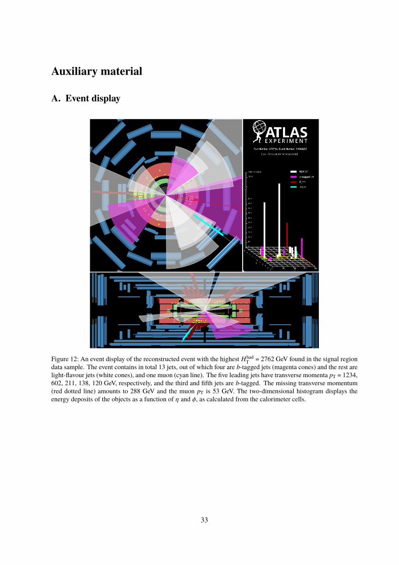
Auxiliary material
A. Event display
Figure 12: An event display of the reconstructed event with the highest HhadT = 2762 GeV found in the signal region
data sample. The event contains in total 13 jets, out of which four are b-tagged jets (magenta cones) and the rest arelight-flavour jets (white cones), and one muon (cyan line). The five leading jets have transverse momenta pT = 1234,602, 211, 138, 120 GeV, respectively, and the third and fifth jets are b-tagged. The missing transverse momentum(red dotted line) amounts to 288 GeV and the muon pT is 53 GeV. The two-dimensional histogram displays theenergy deposits of the objects as a function of η and φ, as calculated from the calorimeter cells.
33

B. Nuisance parameter impact on fitted signal strength
The post-fit values and uncertainties for the most relevant nuisance parameters in the analysis, togetherwith their impact on the signal strength µ for the SM tt̄tt̄ production, are shown in Figure 13. The post-fiterrors are close to 1 if the fitted data do not provide any further constraint on that uncertainty. Conversely, apost-fit error much smaller than 1 indicates a significant reduction with respect to the original uncertainty.The pre-fit (post-fit) effect on µ is calculated by fixing the corresponding nuisance parameter at θ̂ ± ∆θ(±∆θ̂), where θ̂ is the fitted value of the nuisance parameter and ∆θ (∆θ̂) is its pre-fit (post-fit) uncertainty,and performing the fit again. The difference between the default and the modified µ, ∆µ, represents theeffect on µ of this particular systematic uncertainty.
34
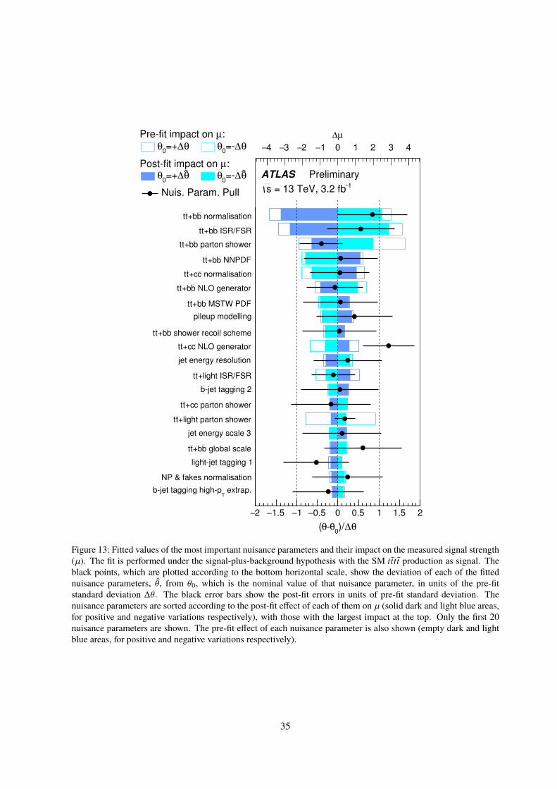
θ∆)/0
θθ(
2− 1.5− 1− 0.5− 0 0.5 1 1.5 2
extrap.
Tbjet tagging highp
NP & fakes normalisation
lightjet tagging 1
global scaleb+btt
jet energy scale 3
+light parton showertt
parton showerc+ctt
bjet tagging 2
+light ISR/FSRtt
jet energy resolution
NLO generatorc+ctt
shower recoil schemeb+btt
pileup modelling
MSTW PDFb+btt
NLO generatorb+btt
normalisationc+ctt
NNPDFb+btt
parton showerb+btt
ISR/FSRb+btt
normalisationb+btt
µ∆
4− 3− 2− 1− 0 1 2 3 4
:µPrefit impact on θ∆=+
0θ θ∆=
0θ
:µPostfit impact on θ∆=+
0θ θ∆=
0θ
Nuis. Param. Pull
ATLAS Preliminary1 = 13 TeV, 3.2 fbs
Figure 13: Fitted values of the most important nuisance parameters and their impact on the measured signal strength(µ). The fit is performed under the signal-plus-background hypothesis with the SM tt̄tt̄ production as signal. Theblack points, which are plotted according to the bottom horizontal scale, show the deviation of each of the fittednuisance parameters, θ̂, from θ0, which is the nominal value of that nuisance parameter, in units of the pre-fitstandard deviation ∆θ. The black error bars show the post-fit errors in units of pre-fit standard deviation. Thenuisance parameters are sorted according to the post-fit effect of each of them on µ (solid dark and light blue areas,for positive and negative variations respectively), with those with the largest impact at the top. Only the first 20nuisance parameters are shown. The pre-fit effect of each nuisance parameter is also shown (empty dark and lightblue areas, for positive and negative variations respectively).
35


![ATLAS NOTE - CERN Document Server · ATLAS NOTE ATLAS-CONF-2016-032 June 16, 2016 ... (2UED/RPP) [34] is also considered. In this model, the compactification of the extra dimensions](https://img.pdfslide.net/doc/110x75/5d4455eb88c9932a398d988e/atlas-note-cern-document-server-atlas-note-atlas-conf-2016-032-june-16-2016.jpg)


![WZ,and ZZProduction - Harvard University · 2016. 7. 29. · ATLAS ATLAS-CONF-2013-021 WZ → ℓνℓℓ [13 fb-1] 8 TeV ATLAS-CONF-2013-020 ZZ → ... 00 50 100 150 200 250 300](https://img.pdfslide.net/doc/110x75/61245d080e3df745330de1e1/wzand-zzproduction-harvard-university-2016-7-29-atlas-atlas-conf-2013-021.jpg)


![ATLAS NOTEcdsweb.cern.ch/record/1406356/files/ATLAS-CONF-2011-161.pdf · 2011. 12. 13. · proton collisiondata samplerecorded with the ATLAS detector[6]in 2011 at a centre-of-massenergy](https://img.pdfslide.net/doc/110x75/60aa6edee6dcf47e7759b25e/atlas-2011-12-13-proton-collisiondata-samplerecorded-with-the-atlas-detector6in.jpg)