Embed Size (px)
Citation preview

Atlas of Climate Scenariosfor Québec Forests
Produced by Ouranos for Ministère des Ressources naturelles and de la Faune du
Québec
Report prepared by
Travis Logan1
Isabelle Charron1
Diane Chaumont1
Daniel Houle12
1OURANOS2 Direction de la Recherche forestière,
Ministère des Ressources naturelles and la Faune du Québec
MARCH 2011

1
Atlas production The Atlas of Climate Scenarios for Québec Forests was mandated by the Direction de la recherche forestière (DRF) at the Ministère des Ressources naturelles et de la Faune du Québec (MRNF). The atlas is intended to be a climate change reference tool for Québec forest managers and other forest stakeholders and is not destined for scientific publication. The indices and variables used in the atlas were jointly chosen by Ouranos and MRNF researchers. The Climate Scenarios group at Ouranos analyzed scenarios, prepared figures and maps, and authored the atlas. The group’s work on the atlas was revised internally by Ouranos researchers, namely Daniel Caya, head of the Climate Science group, and Anne Blondlot from the Impact and Adaptation group for content, layout, and for the quality of the scenarios and results presented.

2
Research Support Research costs were assumed by the Direction de la recherche forestière (DRF) at the Ministère des Ressources naturelles et de la Faune du Québec (MRNF) and the Fonds vert of the Québec government’s Plan d’action 2006–2012 sur les changements climatiques (PACC).
Work was also carried out in collaboration with Natural Resources Canada.
The Ouranos consortium was a key financial partner for a number of the atlas’s authors.
Special thanks to Anne Blondlot of Ouranos for her help in producing the atlas. Paper ISBN: 978-2-923292-11-3 Web ISBN: 978-2-923292-12-0 Legal deposit-Bibliothèque nationale du Québec, 2010 Legal deposit-National Library of Canada, 20120 Recommended bibliographic citation: Logan, T., I. Charron, D. Chaumont, D. Houle. 2011. Atlas of Climate Scenarios for Québec Forests. Ouranos and MRNF. 57 pp + annexes.

3
Contents List of Acronyms .......................................................................................................................... 5 Chapter 1 .................................................................................................................................... 6
1.1 Background ....................................................................................................................... 6 1.2 Introduction ........................................................................................................................ 6
Chapter 2. Methodology .............................................................................................................. 7 2.1 Climate projection selection ............................................................................................... 7
2.1.1. Ensemble simulations from global climate models (GCM).......................................... 7 2.1.2 Ensemble simulations from regional climate models (RCM) ........................................ 8 2.1.3 Cluster analysis .......................................................................................................... 8
2.2 Evaluating climate simulations for the reference period (1971–2000) ................................ 8 2.3 Selection of variables of interest ...................................................................................... 10 2.4 Study area selection ........................................................................................................ 12 2.5 Maps of observed climate normals .................................................................................. 13 2.6 Calculation of projected changes ..................................................................................... 13 2.7 Evolution of anomalies ..................................................................................................... 14
2.7.1 Calculating anomalies ............................................................................................... 14 2.7.2 Displaying anomalies ................................................................................................ 14
2.8 Maps of future changes ................................................................................................... 15 2.8.1 GCM ensemble maps ............................................................................................... 15 2.8.2 RCM ensemble maps ............................................................................................... 15 2.8.3 Interpretation of observed normals and projected changes ....................................... 15
Chapter 3. Mean Temperature .................................................................................................. 16 3.1 Description ...................................................................................................................... 16 3.2 Impact on forest ecosystems ........................................................................................... 17 3.3. Mean temperature results ............................................................................................... 18
3.3.1 Normals and anomalies ............................................................................................ 18 3.3.2 Projected changes .................................................................................................... 18
Chapter 4. Total Precipitation .................................................................................................... 21 4.1 Description ...................................................................................................................... 21 4.2 Impact on forest ecosystems ........................................................................................... 22 4.3 Total precipitation results ................................................................................................. 23
4.3.1 Normals and anomalies ............................................................................................ 23 4.3.2 Projected changes .................................................................................................... 23
Chapter 5. Snowfall Precipitation ............................................................................................... 26 5.1 Description ...................................................................................................................... 26 5.2 Impact on forest ecosystems ........................................................................................... 27 5.3 Snowfall precipitation results ........................................................................................... 28
5.3.1 Normals and anomalies ............................................................................................ 28 5.3.2 Projected changes .................................................................................................... 28
Chapter 6. Freeze/Thaw Events ................................................................................................ 31 6.1 Description ...................................................................................................................... 31 6.2 Impact on forest ecosystems ........................................................................................... 32 6.3 Freeze/thaw event results ................................................................................................ 34
6.3.1 Normals and anomalies ............................................................................................ 34 6.3.2. Projected changes ................................................................................................... 34
Chapter 7. Growing Degree-Days ............................................................................................. 38 7.1 Description ...................................................................................................................... 38 7.2 Impact on forest ecosystems ........................................................................................... 39

4
7.3 Growing degree-day results ............................................................................................. 39 7.3.1 Normals and anomalies ............................................................................................ 39 7.3.2 Projected changes .................................................................................................... 39
Chapter 8. Growing Season length ............................................................................................ 41 8.1 Description ...................................................................................................................... 41 8.2 Impact on forest ecosystems ........................................................................................... 42 8.3 Growing season length results ......................................................................................... 42
8.3.1 Normals and anomalies ............................................................................................ 42 8.3.2 Projected changes .................................................................................................... 42
Chapter 9. Canadian Drought Code .......................................................................................... 44 9.1 Description ...................................................................................................................... 44 9.2 Impact on forest ecosystems ........................................................................................... 45 9.3 Canadian drought code results ........................................................................................ 45
9.3.1 Normals and anomalies ............................................................................................ 45 9.3.2 Projected changes .................................................................................................... 45
Conclusions ............................................................................................................................... 56 References ................................................................................................................................ 57 Annexes Annex 1 Maps of observed climate normals: all seasons ........................................................... 64 Annex 2 Evolution of anomalies: all seasons ............................................................................. 73 Annex 3 Maps of projected changes: all seasons ...................................................................... 82 Annex 4 Detailed methodology ................................................................................................ 116 A4.1 Cluster analysis ............................................................................................................... 116 A4.2 Evaluation of the climate models for the period 1971-2000 ............................................. 120 A4.3 Results of the climate model evaluation .......................................................................... 122 References .............................................................................................................................. 132 Note: Figures presented in this version originate from the French version of the Atlas and were not translated here. English figure captions describe the axes and legends of the figures.

5
List of Acronyms
AMNO domain Canadian regional climate model domain for North America on a grid 182 points by 174 points, with 45 km tiles true at 60oN
CRCM Canadian Regional Climate Model
DJF December, January, February (winter)
DRF Direction de la recherche forestière GCM Global Climate Model GDD Growing Degree-Days GHG Greenhouse gas GSL Growing season length IPCC Intergovernmental Panel on Climate Change JJA June, July, August (summer) MAM March, April, May (spring) MRNF Ministère des Ressources naturelles and de la Faune du Québec NARCCAP North American Regional Climate Change Assessment Program NLWIS National Land and Water Information Service NRCan Natural Resources Canada PACC Plan d’action sur les changements climatiques (Québec government climate
change action plan) PCMDI Program for Climate Model Diagnosis and Intercomparison RCM Regional climate model SON September, October, November (fall) SRES Special Report on Emissions Scenarios WMO World Meteorological Organization

6
Chapter 1 1.1 Background The Direction de la recherche forestière (DRF) at the Ministère des Ressources naturelles et de la Faune du Québec (MRNF) tasked Ouranos with producing an atlas of climate scenarios to provide an overview of anticipated changes for a number of variables and indices of interest to Québec forests. These indices and variables, which form the basis of the climate information set out here, were deemed most relevant to the growth and dynamics of Québec forests by DRF researchers in collaboration with Ouranos. 1.2 Introduction Climate scenarios are used by impact and adaptation projects to analyze potential impacts of climate change on forests. These scenarios are constructed using climate models, which are numerical representations of the climate system based on equations governing the physical processes of climate components. Climate models are therefore unique tools enabling the reproduction of a complex set of processes responsible for climate evolution (Murphy et al. 2004). Until recently, climate projections largely came from global models (GCM), which have a spatial resolution of approximately 200 km to 300 km. This resolution is often insufficient for climate change impact and adaptation applications and the downscaling of global projections toward a resolution better suited to regional model applications has proven to be useful, if not indispensable. Regional climate simulation is one of the strengths of the Ouranos consortium and its research partners, who have helped develop the Canadian Regional Climate Model (CRCM; Caya and Laprise 1999). This model, like other regional climate models (RCM), is based on the conservation of energy, mass, and momentum to generate temporal series of physically coherent climate variables. Regional models therefore respect the same physical principles as GCM, but are concentrated on a reduced spatial domain, meaning that climate simulations can be produced at a higher spatial resolution (approximately 45 km for the current CRCM1
).
1 CRCM resolution will be increased in the near future.
Consequently, in order to compare variables from global models with a coarser resolution to variables from regional signals of a finer resolution, the data presented in this atlas are based both on an ensemble of global climate simulations—made available by the Program for Climate Model Diagnosis and Intercomparison (PCMDI) project —as well as an ensemble of regional simulations produced by Ouranos and its partners. Moreover, using both ensembles of simulations allows the sources of uncertainty in the climate projections to be better identified and evaluated. Recent climate change impact and adaptation studies show that analyses using results from an ensemble of climate simulations have, to date, provided the best estimate of a simulated climate (Gleckler et al. 2008). More specifically, the median or the mean of a large ensemble of GCM or RCM simulations produces more consistent results compared to reference data on a range of climate variables in several parts of the world. What’s more, using an ensemble of simulations means that climate projection uncertainty can be evaluated and allows decision makers to gauge the level of confidence that can be placed in calculated median or mean changes. This document first briefly describes the methodology used to select the indices and variables used for the atlas and to select climate simulations. The seven chapters below set out in turn the indices and variables of interest. Each chapter contains the following information: 1) a description of the index along with a definition, the observed normals for the reference period (1971–2000), and the projected change in the index over time, 2) background information on the importance of the index for forest ecosystems, 3) a description and maps of changes and uncertainties projected by regional simulations for the 2050 horizon and by global simulations for the 2050 and 2090 horizons. The principal portion of the document describes observed normals and projected changes for the seasons deemed most relevant. However, maps for all seasons have been produced and are presented in three annexes. Respectively, the annexes comprise: 1) maps of observed climate normals for the reference period for all seasons, 2) projected changes over time for all seasons, and 3) Maps of average changes projected by the complete RCM and GCM ensemble datasets for all seasons. A fourth annex is also included, which provides a detailed

7
methodology for the selection and evaluation of the climate simulations. Chapter 2. Methodology 2.1 Climate projection selection 2.1.1. Ensemble simulations from global climate models (GCM) An ensemble of 71 global simulations (Table 1) was used to produce this atlas. Data for this ensemble came from the Program for Climate Model Diagnosis and Intercomparison (PCMDI,
Meehl et al. 2007) archive, which provides researchers with a large number of GCM simulations produced by different modelling centres around the world. Simulated data are available for three GHG scenarios stemming from the Special Report on Emissions Scenarios (SRES: A1b, A2, and B1; Nakicenovic et al. 2000). Figure 2.1b shows the change in global average temperature according to an ensemble of simulations arising from a number of GHG emissions scenarios. These emissions scenarios were endorsed by the IPCC and formed the basis of the last IPCC evaluation report published in 2007.
a) b) Figure 2.1 a) Worldwide GHG emissions (CO2, CH4, N2O, and fluorinated gases) illustrating six SRES scenarios (coloured lines) and b) Change in mean global temperature according to GCM simulations grouped together by SRES GHG scenario (Source: IPCC 2007, WG1-AR4).
8
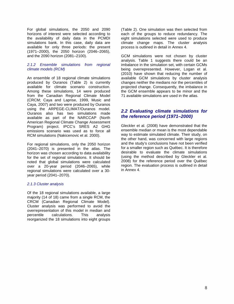
For global simulations, the 2050 and 2090 horizons of interest were selected according to the availability of daily data in the PCMDI simulations bank. In this case, daily data are available for only three periods: the present (1971–2000), the 2050 horizon (2046–2065), and the 2090 horizon (2081–2100). 2.1.2 Ensemble simulations from regional climate models (RCM) An ensemble of 18 regional climate simulations produced by Ouranos (Table 2) is currently available for climate scenario construction. Among these simulations, 14 were produced from the Canadian Regional Climate Model (CRCM; Caya and Laprise, 1999, Music and Caya, 2007) and two were produced by Ouranos using the ARPEGE-CLIMAT/Ouranos model. Ouranos also has two simulations made available as part of the NARCCAP (North American Regional Climate Change Assessment Program) project. IPCC’s SRES A2 GHG emissions scenario was used as to force all RCM simulations (Nakicenovic et al. 2000). For regional simulations, only the 2050 horizon (2041–2070) is presented in the atlas. The horizon was chosen according to data availability for the set of regional simulations. It should be noted that global simulations were calculated over a 20-year period (2046–2065), while regional simulations were calculated over a 30-year period (2041–2070). 2.1.3 Cluster analysis Of the 18 regional simulations available, a large majority (14 of 18) came from a single RCM, the CRCM (Canadian Regional Climate Model). Cluster analysis was performed to avoid the overrepresentation of this model in median and percentile calculations. This analysis reorganized the 18 simulations into eight groups
(Table 2). One simulation was then selected from each of the groups to reduce redundancy. The eight simulations selected were used to produce climate change maps. The cluster analysis process is outlined in detail in Annex 4. GCM simulations were not chosen by cluster analysis. Table 1 suggests there could be an imbalance in the simulation set, with certain GCMs being overrepresented. However, Logan et al. (2010) have shown that reducing the number of available GCM simulations by cluster analysis changes neither the medians nor the percentiles of projected change. Consequently, the imbalance in the GCM ensemble appears to be minor and the 71 available simulations are used in the atlas. 2.2 Evaluating climate simulations for the reference period (1971–2000)
Gleckler et al. (2008) have demonstrated that the ensemble median or mean is the most dependable way to estimate simulated climate. Their study, on the other hand, was concerned with large regions and the study’s conclusions have not been verified for a smaller region such as Québec. It is therefore desirable to evaluate the climate simulations (using the method described by Gleckler et al. 2008) for the reference period over the Québec region. The evaluation process is outlined in detail in Annex 4.

9
Table 1. Ensemble of 71 selected GCM simulations chosen for the atlas
Model
Member
SRES
Model
Member
SRES
CCCMA_CGCM3_1 Run1 SRESA1B MIROC3_2_HIRES Run1 SRESA1B CCCMA_CGCM3_1 Run1 SRESA2 MIROC3_2_HIRES Run1 SRESB1 CCCMA_CGCM3_1 Run1 SRESB1 MIROC3_2_MEDRES Run1 SRESA1B CCCMA_CGCM3_1 Run2 SRESA1B MIROC3_2_MEDRES Run1 SRESA2 CCCMA_CGCM3_1 Run2 SRESA2 MIROC3_2_MEDRES Run1 SRESB1 CCCMA_CGCM3_1 Run2 SRESB1 MIROC3_2_MEDRES Run2 SRESA1B CCCMA_CGCM3_1 Run3 SRESA1B MIROC3_2_MEDRES Run2 SRESA2 CCCMA_CGCM3_1 Run3 SRESA2 MIROC3_2_MEDRES Run2 SRESB1 CCCMA_CGCM3_1 Run3 SRESB1 MIUB_ECHO_G Run1 SRESA1B
CCCMA_CGCM3_1_t63 Run1 SRESA1B MIUB_ECHO_G Run1 SRESA2 CCCMA_CGCM3_1_t63 Run1 SRESB1 MIUB_ECHO_G Run1 SRESB1
CNRM_CM3 Run1 SRESA1B MIUB_ECHO_G Run2 SRESA1B CNRM_CM3 Run1 SRESA2 MIUB_ECHO_G Run2 SRESA2 CNRM_CM3 Run1 SRESB1 MIUB_ECHO_G Run2 SRESB1
CSIRO_MK3_0 Run1 SRESA1B MIUB_ECHO_G Run3 SRESA1B CSIRO_MK3_0 Run1 SRESA2 MIUB_ECHO_G Run3 SRESA2 CSIRO_MK3_0 Run1 SRESB1 MIUB_ECHO_G Run3 SRESB1 CSIRO_MK3_5 Run1 SRESA1B MPI_ECHAM5 Run1 SRESA2 CSIRO_MK3_5 Run1 SRESA2 MPI_ECHAM5 Run1 SRESB1 CSIRO_MK3_5 Run1 SRESB1 MPI_ECHAM5 Run4 SRESA1B GFDL_CM2_0 Run1 SRESA1B MRI_CGCM2_3_2A Run1 SRESA1B GFDL_CM2_0 Run1 SRESA2 MRI_CGCM2_3_2A Run1 SRESA2 GFDL_CM2_0 Run1 SRESB1 MRI_CGCM2_3_2A Run1 SRESB1
GISS_AOM Run1 SRESA1B MRI_CGCM2_3_2A Run2 SRESA1B GISS_AOM Run1 SRESB1 MRI_CGCM2_3_2A Run2 SRESA2
IAP_FGOALS1_0_G Run1 SRESA1B MRI_CGCM2_3_2A Run2 SRESB1 IAP_FGOALS1_0_G Run1 SRESB1 MRI_CGCM2_3_2A Run3 SRESA1B IAP_FGOALS1_0_G Run2 SRESA1B MRI_CGCM2_3_2A Run3 SRESA2 IAP_FGOALS1_0_G Run2 SRESB1 MRI_CGCM2_3_2A Run3 SRESB1 IAP_FGOALS1_0_G Run3 SRESA1B MRI_CGCM2_3_2A Run4 SRESA1B IAP_FGOALS1_0_G Run3 SRESB1 MRI_CGCM2_3_2A Run4 SRESA2
INGV_ECHAM4 Run1 SRESA1B MRI_CGCM2_3_2A Run4 SRESB1 INGV_ECHAM4 Run1 SRESA2 MRI_CGCM2_3_2A Run5 SRESA1B
IPSL_CM4 Run1 SRESA1B MRI_CGCM2_3_2A Run5 SRESA2 IPSL_CM4 Run1 SRESA2 MRI_CGCM2_3_2A Run5 SRESB1 IPSL_CM4 Run1 SRESB1
10
Table 2. Ensemble of selected RCM simulations chosen for the atlas
RCM
Domain
Pilot
Member
SRES
Source
CRMC4.1.1 Qc CGCM3 4 A2 OURANOS CRMC4.1.1 Qc CGCM3 5 A2 OURANOS CRMC4.2.0 AMNO CGCM2 3 A2 OURANOS CRMC4.2.0 AMNO CGCM3 4 A2 OURANOS CRMC4.2.0 AMNO CGCM3 5 A2 OURANOS CRMC4.2.3 AMNO CGCM3 1 A2 CRMC4.2.3 AMNO CGCM3 2 A2 OURANOS CRMC4.2.3 AMNO CGCM3 3 A2 OURANOS CRMC4.2.3 AMNO CGCM3 4 A2 OURANOS CRMC4.2.3 AMNO CGCM3 5 A2 OURANOS CRMC4.2.3 Qc CGCM3 4 A2 OURANOS CRMC4.2.3 Qc CGCM3 5 A2 OURANOS CRMC4.2.3 AMNO ECHAM5 A2 OURANOS CRMC4.2.3 Qc ECHAM5 A2 OURANOS ARPEGE-
CLIMAT/Ouranos AMNO NA 1 A2 OURANOS
ARPEGE-CLIMAT/Ouranos
AMNO NA 2 A2 OURANOS
HRM3 NARCCAP HADCM3 A2 NARCCAP RCM3 NARCCAP CGCM3 A2 NARCCAP
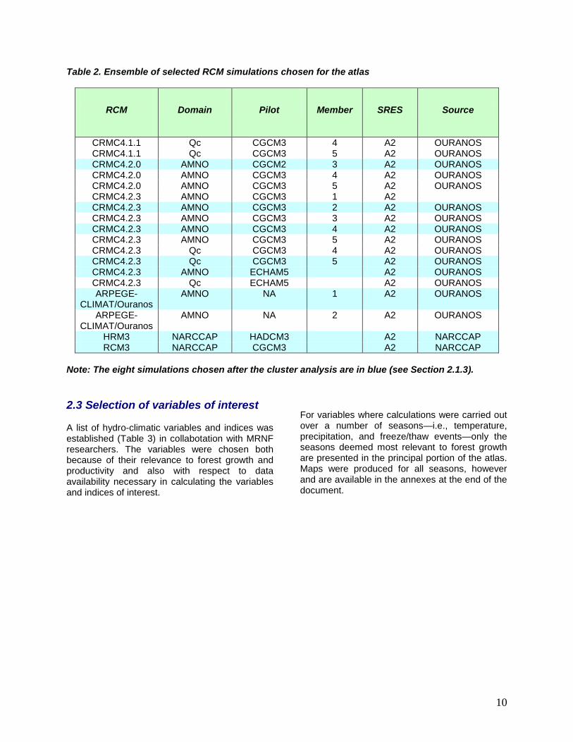
Note: The eight simulations chosen after the cluster analysis are in blue (see Section 2.1.3). 2.3 Selection of variables of interest A list of hydro-climatic variables and indices was established (Table 3) in collabotation with MRNF researchers. The variables were chosen both because of their relevance to forest growth and productivity and also with respect to data availability necessary in calculating the variables and indices of interest.
For variables where calculations were carried out over a number of seasons—i.e., temperature, precipitation, and freeze/thaw events—only the seasons deemed most relevant to forest growth are presented in the principal portion of the atlas. Maps were produced for all seasons, however and are available in the annexes at the end of the document.

11
Table 3. Summary of selected hydro-climatic variables and indices
Variable or Index Description
Mean temperature The mean temperature calculated on a daily basis
Minimum temperature1 The minimum daily temperature calculated on a daily basis
Maximum temperature1 The maximum daily temperature calculated on a daily basis Total precipitation Total daily precipitation in millimetres falling in liquid and snow form
Snowfall Daily precipitation in millimetres falling as snow
Freeze/thaw events
Days with a freeze/thaw event are days when the temperature oscillates above and below 0˚C in 24 hours. Specifically, a daily freeze/thaw event is observed when, within a 24-hour period, the minimum recorded temperature is below 0˚C and the maximum recorded temperature is above 0˚C.
Growing degree-days
The difference in degrees Celsius that separates the mean daily temperature from a base value of 5˚C. If the difference is equal to or less than 5˚C, the day has zero growing degree-days. Daily values for degree-days are accumulated on an annual basis. The base value of 5˚C was established according to plant growth and development relationships. The basic assumption is that plants will grow only if the ambient temperature is greater than this minimum value. There is also presumed to be a quasi-linear relationship between growth increases and temperature increases or the accumulation of heat energy (Schenk 1996; Loehle 1998; Bonhomme 2000).
Growing season length
The growing season starts when the mean daily temperature is equal to or greater than 5˚C for five consecutive days starting March 1. It ends when the mean daily temperature is below -2˚C starting August 1. This is the definition used by Natural Resources Canada. It is important to note that the growing season as defined here is a season of potential growth based strictly on a temperature index. It represents a potential increase in growth that does not necessarily correspond to the actual growing season for a particular species.
Canadian drought code
The Canadian drought code is intended to be an empirical evaluation of the mean water content of forest soil. It is calculated based on combined daily temperatures and precipitation from April 1 to October 31, using the method proposed by Turner (1972).
1 Results for changes in minimum and maximum temperatures are outlined in Annexes 1 to 3.

12
2.4 Study area selection Climate models all have different grids and resolutions. It is therefore necessary to establish a common study area and reference grid in order to consistently evaluate the variables produced by the models (Figure 2.2). For the GCMs, the common grid chosen is the section of the Canadian global model grid (CGCM3 T47) that covers Québec (Figure 2.2a). Variables for all GCMs were therefore interpolated (using the
“nearest neighbour” method) to this grid. For the RCMs, the common grid chosen is the portion of the Canadian regional model (AMNO domain) that covers Québec (Figure 2.2b). Here too, variables for all regional models were interpolated using the “nearest neighbour” method to this grid. In both cases, only tiles with more than 50% of land according to the land-sea mask were included. To map projected changes, the value at the grid point nearest the reference grid centroid is chosen.
a) b)
Figure 2.2 Reference grid for (a) Global climate models (CGCM3 t47) and (b) Regional climate models (RCMC4, AMNO domain) over Québec. Only points with more than 50% of land were used in the analysis.

13
2.5 Maps of observed climate normals The World Meteorological Organization (WMO) standard for defining climate normals is the mean climate state over a 30 year period. For the reference period, the mean for 1971 to 2000 is generally used. Observed normals (not coming from a climate model) provide a comparison or reference base by which changes projected by various models can be evaluated (see Section 2.8.3). Normals are calculated using daily temperature and precipitation data. Data used in this atlas come from the NLWIS (National Land and Water Information Service) and are provided on a regular grid with a spatial resolution of 10 km × 10 km covering Canada south of 60°N. Seasonal values for each of the variables and indices of interest were calculated for each grid point and for each year. The mean 30-year value was then mapped. An example of mean winter and summer temperatures can be found in Figure 2.3. 2.6 Calculation of projected changes
Changes or deltas (Δ) projected by each simulation were calculated in one of the following ways: By the difference
reffutdiff valuevalue −=∆ (1) or by the percentage
)1/(100 −=∆ reffutprct valuevalue (2)
Valuefut is the mean of a variable for the future 30 year period for a given simulation and valueref is the 30 year mean for the reference period for the same simulation. Changes in total precipitation and snowfall are calculated using Equation 2 for the principal portion of the atlas (changes in mm using Equation 1 are available in Annex 3), while changes for all other indices are calculated using Equation 1.
a) b)
Figure 2.3 Observed normals for mean temperature (in ˚C) for the reference period (1971–2000) for (a) winter (DJF) and (b) summer (JJA) months.

14
2.7 Evolution of anomalies 2.7.1 Calculating anomalies Changes in variables over time are often presented as anomalies. Annual or seasonal anomalies for a variable (anom_diffi or anom_prcti) were calculated for each simulation: By the difference
refii valuevaluediffanom −=_ (3)
or by the percentage
−=
ref
refii value
valuevalueprctanom 100_ (4)
Valuei is the value of the variable for a year or season and valueref is the mean of the value for the 30 year reference period for the same simulation. Values represent spatial means for the entire Québec reference grid. 2.7.2 Displaying anomalies For the GCM simulations, the median anomaly value of the ensemble of 71 simulations was
calculated for each year. A confidence interval around the median, representing the difference between the 10th and 90th percentiles of the 71 values for each year was also calculated. Figure 2.4 shows an example of the evolution of anomalies for mean winter and summer temperatures for the period from 1971 to 2100. For the RCM ensemble, the median anomaly value for the eight regional simulations is shown in the same figure (Figure 2.4). Given the lower number of simulations available for the RCMs, the interval around the median is not shown. It should be noted that this smaller number of simulations is responsible for fluctuations in the median curve for RCM anomalies, which are greater compared to the GCM anomalies. Moreover, given the different number of simulations for the two types of models, statistical comparison cannot be made between their medians. Nevertheless, for the vast majority of variables, the trajectories of GCM and RCM curves are parallel and the GCM envelope of variability encompasses RCM fluctuations. Consequently, although this document only presents projected RCM changes for the 2050 horizon, the GCM curves allow us to gauge the possible scale of mean changes for regional models for the 2090 horizon.
Figure 2.4 Evolution of anomalies for mean temperature from 1971 to 2100 calculated the selected GCM (nGCM=71) and RCM (nRCM=8) ensemble.

15
2.8 Maps of future changes 2.8.1 GCM ensemble maps
For each simulation, climate indices and variables were calculated for the reference period and future horizons. These calculations were made for each grid point and the mean seasonal deltas for each simulation were then calculated using equations 1 and 2. Calculated deltas were transferred to the reference grid (Figure 2.2a) to produce the maps. For each GCM reference grid tile, the median value of the ensemble of projected changes was mapped for the 2050 and 2090 horizons. In order to show the uncertainty surrounding climate change projections, two additional maps showing the 10th and 90th percentiles of the projected changes were also produced. 2.8.2 RCM ensemble maps As for the GCM ensemble, the median value of projected changes was mapped for each RCM
reference grid tile (Figure 2.2b) for the 2050 horizon. Maps showing the 10th and 90th percentiles of the changes were also produced. 2.8.3 Interpretation of observed normals and projected changes Figure 2.5 presents an example of observed normals for total winter precipitation for the reference period and median changes in total winter precipitation projected for the 2050 horizon by the RCMs. Note that observed normals are given in millimetres, while changes are presented as a percentage (calculated using Equation 2). Consequently, in order to interpret the extent of median projected changes, percentages must be converted to millimetres. For example, for the extreme south of Québec, observed normals range from 200 mm (in yellow) to 250 mm (in light blue). For the same area, median projected changes are close to 20%. The maps therefore project increases in total precipitation between 40 mm to 50 mm for the 2050 horizon for the area.
a) b)
Figure 2.5 a) Observed normals of total winter precipitation (in mm) for the reference period (1971–2000) and (b) projected median change in winter total precipitation (as a percentage) by the regional climate models for the 2050 horizon.

16
Chapter 3. Mean Temperature3.1 Description
DEFINITION Daily mean temperature
FORMULA
Tmeasea = Nsea
Nsea
i iTmea∑
Tmeasea: seasonal mean temperature (sea) Tmeai: daily mean temperature (i) i: a given day Nsea: the total number of days in a season
Figure 3.2 Evolution of anomalies (see Section 2.7) in mean temperature from 1971 to 2100 calculated for the selected GCM (nGCM=71) and RCM (nRCM=8) ensembles. Note that the small number of RCM simulations is responsible for the larger fluctuations in their median curve. Also, given the different number of RCM and GCM simulations, no statistical comparison between the medians can be performed.
Figure 3.1 Observed normals of mean temperature (°C) for the reference period (1971–2000) for winter (DJF) and summer (JJA). Values were calculated using NLWIS data.
IMPACT ON FOREST ECOSYSTEMS • Metabolism and growth • Phenology • Distribution and migration • Frequency of natural disturbances • Biogeochemical cycles

17
3.2 Impact on forest ecosystems Temperature is the climate variable most often used to describe future changes to the environment. A number of studies have shown that a global increase in temperatures will have an impact on a large number of terrestrial ecosystems (e.g., Walther et al. 2002, Parmesan and Yohe 2003; Woodward et al. 2004; Hamann and Wang 2006, Parmesan 2006; Millar et al. 2007; Canadell and Raupach 2008; Allen et al. 2010). Various reasons explain why temperature is often used. First, temperature is one of the most intuitive variables. Second, temperature data is relatively easy to obtain, and often for long periods. Third, temperature is often directly correlated to other climate indices that can be more difficult to quantify and conceptualize (such as growing degree-days and the drought index). Temperature has a direct influence on a number of biological processes, notably species metabolism and growth (Myneni et al. 1997; Coulombe et al. 2009; Leblanc and Terrell 2009; Deslauriers et al. 2008; Huang et al. 2010). For instance, studies on boreal forest conifers show a significant correlation between temperature and precipitation and a number of growth indices: cell production, annual growth, and forest productivity (Bonan and Shugart 1989; Brooks et al. 1998; Wang et al. 2002; Wilmking et al. 2004; Danby and Hik 2007; Briffa et al. 2008; Kurtz et al. 2008). Temperature has a definite impact on phenology, influencing the moment of budding and the date and duration of flowering (Menzel et al. 2003; Root et al. 2003; Parmesan 2006). Temperature mainly has an impact on the accumulation of growing degree-days, setting a threshold for certain phenological events. The direct influence of temperature on species growth and phenology has an impact on competition mechanisms. This could influence plant distribution and migration (Lescop-Sinclair and Payette 1995; Kullman 2001; Shafer et al. 2001; Root et al. 2003; Woodward et al. 2004; Thuiller et al. 2005; Parmesan 2006; Boisvenue and Running 2006; Harsch et al. 2009). For example, at the southern limit of the distribution areas, forest distribution and composition might undergo certain changes since species migrating northward should be better adapted to the new
temperatures and could replace certain species there. On the other hand, these changes are not a given: there are a number of factors involved, including dispersal distance and rate, the frequency of natural disturbances, and soil characteristics (Loehle 1998; Goldblum and Rigg 2005). The influence of temperature is clearer at the northern limit of the distribution areas. A number of dendrochronological studies show that at the northern limit of the distributions, tree growth is significantly correlated to the mean temperature of the growing season (Garfinkel and Brubaker 1980; Briffa et al. 2008; McDonald et al. 2008). This correlation between tree growth and temperature suggests that the northern tree line of the boreal forest is limited by temperature and that a temperature increase would result in better individual growth and survival and even a migration of trees to the north (MacDonald et al. 2000; Kullman 2001; MacDonald et al. 2008; Harsch et al. 2009). Recent studies based on future climate scenarios also project a general shift to the north in the distribution of a number of species in North America (Sturm et al. 2001; Haman and Wang 2006; McKenney et al. 2007). On the other hand, although mean temperature has increased globally over the past decade, a shift in the tree line to the north has not been observed everywhere (Wilmking et al. 2004; Harsch et al. 2009). Certain communities may have migrated, but others have not shifted or have even moved slightly to the south (Harsch et al. 2009). This is due in part to the fact that local temperature changes may be different to mean temperature changes, since temperature can vary on a regional spatial scale. Moreover, although temperature is partly responsible for species migration, a number of other factors, such as precipitation, geology, and natural disturbances can also influence tree response and migration (Larsen and MacDonald 1995; Lescop-Sinclair and Payette 1995; Brooks et al. 1998; Lloyd 2005; Wang et al. 2006). Population shifts to the south are, for example, often associated with disturbances such as forest fires and insect outbreaks (Harsch et al. 2009). This is true for white spruce in Québec, where the tree line on the Labrador coast moved north due to a temperature increase, while the tree line close to the centre of the province, where forest fires were frequent, shifted south (Payette 2007).
18
Temperature changes also have an impact on the frequency and intensity of natural disturbances such as insects and fires (Stocks et al. 1998, Logan et al. 2003; Battisti et al. 2005; Flannigan et al. 2005, Woods et al. 2005; Hamann and Wang 2006; Westerling et al. 2006; Kurtz et al. 2008; Lindner et al. 2010). An increase in temperatures partly explains a number of recent insect outbreaks. This is the case, for example, with the mountain pine beetle in British Columbia, where an increase in mean temperature is helping favour the development and dispersion of the species, while the absence of very cold winter temperatures is helping larvae to survive (Hamann and Wang 2006). Temperature could also influence fires in a number of ways. First, studies show that across Canada an increase in temperatures is associated with an increase in the annual area burned (Gillett et al. 2004; Flannigan et al. 2005; Girardin et al. 2006b). These studies suggest that, over the long term, temperature is the best predictor of the annual area burned. Moreover, a general increase in temperatures could be correlated with a longer fire season, particularly if the increase is correlated with a decrease in winter precipitation and increased soil drought (Wotton and Flannigan 1993; Wotton et al. 2003). On the other hand, fires are also greatly influenced by precipitation and the interaction between the two variables can be complex. For instance, in Québec, studies show that increased precipitation over the past 150 years appears to have countered the effect of a simultaneous temperature increase, resulting in less frequent fires (Bergeron and Archambault 1993; Bergeron et al. 2001; Flannigan et al. 2005). Lastly, a temperature rise will have an influence on the carbon cycle even if the actual impact is hard to predict. On the one hand, increased tree growth and more productive forest ecosystems combined with tree migration to the north (replacing the tundra) would increase worldwide carbon sequestration (Koerner 2000; Kurtz et al. 2008; MacDonald et al. 2008). However an increase in forest fires resulting in the loss of forest ecosystems would reduce carbon sequestration (Kurtz et al. 2008). It is also interesting to note that the various processes can have opposing effects on global warming. On the one hand, increased tree growth and increased carbon sequestration should slow global warming, but a loss of forest surfaces and a
decrease in carbon sequestration could accelerate it (Foley et al. 2003). 3.3. Mean temperature results 3.3.1 Normals and anomalies Figure 3.1 shows the observed normals of mean temperature (°C) for the reference period (1971–2000) for winter (DJF) and summer (JJA). Figure 3.2 shows the evolution of anomalies (see Section 2.7) for mean temperature from 1971 to 2100 calculated for the selected GCM (nGCM=71) and RCM (nRCM=8) ensembles. 3.3.2 Projected changes Winter (DJF) Figure 3.3 shows the changes in mean temperature projected by the global and regional ensembles for the 2050 and 2090 horizons. Warming is greatest in the centre and north of the province for both horizons for both the regional and global ensembles. More specifically, the median change in mean temperatures projected for the 2050 horizon by RCM and GCM ensembles varies between 3°C and 5°C (Figure 3.3a, b). Warming is slightly higher around Hudson Bay. The values for the 10th and 90th GCM percentiles are higher than for the RCMs. For the 2090 horizon (Figure 3.3c), the GCMs project a median change in mean temperature of 5°C to 9°C. Warming follows a south–north gradient, with higher values for the north of Québec. Summer (JJA) Median summer temperature changes for the 2050 horizon are more uniform and range from 1.8°C to 2.7°C according to regional models (Figure 3.4a) and from 1.7°C to 2.2°C according to global models (Figure 3.4b). The temperature gradient is the inverse of the gradient projected for the winter season, with higher values in the south of Québec for both horizons. For the 2090 horizon (Figure 3.4c), the projected median change in temperature for the GCMs is 2°C to 3.5°C. There is also a north–south gradient, with higher values in the south.

19
a) RCM 2050 Winter (DJF)
b) GCM 2050
c) GCM 2090
Figure 3.3 Projected change in mean daily winter temperature (in °C) between the reference period (1971–2000) and (a) the 2050 horizon, calculated using the ensemble of RCM simulations, and horizons (b) 2050 and (c) 2090, calculated using the ensemble of GCM simulations. The centre column shows the median change, while the first and last columns show the 10th and 90th percentiles.

20
a) RCM 2050 Summer (JJA)
b) GCM 2050
c) GCM 2090
Figure 3.4 Projected change in mean daily summer temperature (in °C) between the reference period (1971–2000) and (a) the 2050 horizon, calculated using the ensemble of RCM simulations, and horizons (b) 2050 and (c) 2090, calculated using the ensemble of GCM simulations. The centre column shows the median change, while the first and last columns show the 10th and 90th percentiles.
21
Chapter 4. Total Precipitation 4.1 Description
DEFINITION Accumulation of total daily precipitation in millimetres that falls in liquid or snow form.
FORMULA
Ptotalsea = ∑Nsea
i iPt
Ptotalsea: total precipitation in mm that falls in rain or snow form during a season Pti: total daily precipitation in mm that falls in rain or snow form i: a given day Nsea: the total number of days in a season
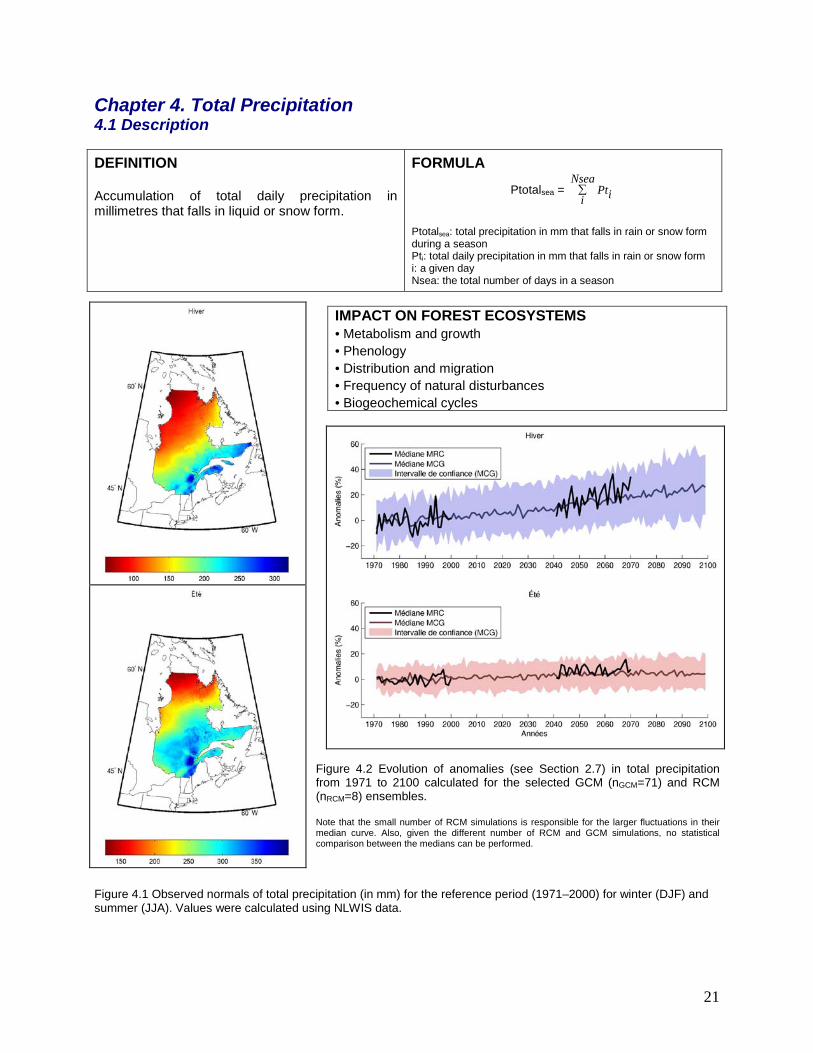
Figure 4.2 Evolution of anomalies (see Section 2.7) in total precipitation from 1971 to 2100 calculated for the selected GCM (nGCM=71) and RCM (nRCM=8) ensembles. Note that the small number of RCM simulations is responsible for the larger fluctuations in their median curve. Also, given the different number of RCM and GCM simulations, no statistical comparison between the medians can be performed.
Figure 4.1 Observed normals of total precipitation (in mm) for the reference period (1971–2000) for winter (DJF) and summer (JJA). Values were calculated using NLWIS data.
IMPACT ON FOREST ECOSYSTEMS • Metabolism and growth • Phenology • Distribution and migration • Frequency of natural disturbances • Biogeochemical cycles

22
4.2 Impact on forest ecosystems As with temperature, precipitation has an influence on plant distribution and growth. Consequently these two variables are often used together in climate change impact studies (Bakkenes et al. 2002; Woodward et al. 2004). The seasonality of precipitation is crucial. In a temperate climate, with a relatively short growing season, adequate precipitation over the summer will have a positive influence on plant growth and survival. The impact of precipitation is particularly clear on plant growth at the start of the season, when a shortage of liquid precipitation will slow or even stop growth (Hoffer and Tardif 2009; Leblanc and Terrell 2009). This close correlation is relatively easy to study by looking at the breadth and density of annual growth rings. Using this information, researchers can infer historical precipitation sequences and, in particular, track drought episodes (Fritz 2001; Tardif and Bergeron 1997; Hoffer and Tardif 2009; Girardin et al. 2004a, b, 2006b). Conversely, during the winter season, too much liquid precipitation, which tends to be correlated with milder temperatures, can have a negative impact on plant survival. This impact is related to the fact that rain increases the amount of water in the soil, thereby making the soil more likely to freeze, especially if there is little thermal insulation provided by the snow cover (Henry 2008; Zhang et al. 2008; Morgner et al. 2010). Soil freezing can damage plant roots, particularly roots of young seedlings and species with shallow roots (Tierney et al. 2001; Cleavitt et al. 2008, Auclair et al. 2010). The spatial distribution of species is partly correlated to precipitation, although temperature also plays an important role in the spread of distribution areas (Dang and Lieffers 1989; Flannigan and Woodward 1994; Briffa et al. 2008). The relative importance of precipitation and temperature can be difficult to estimate and can vary according to the environment or the species. For example, a study looking at the Douglas fir (Pseudotsuga menziesii) in British Columbia shows that climate response varies within the same species according to the local conditions in which individuals belonging to a population find themselves. In this case, populations growing in a relatively warm, dry climate have growth patterns correlated with annual precipitation. Conversely, populations
growing at high altitudes in more humid, colder climates have growth patterns correlated with snow precipitation and with winter and annual temperatures (Greisbauer and Green 2010). Moreover, in the same environment, the same species can have a different response to changes in temperature and precipitation. In the boreal forest, for instance, the radial growth of the black spruce is, in certain environments, particularly well correlated with total precipitation (Dang and Lieffers 1989; Brooks et al. 1998) and, in other environments, more correlated with temperature (Hoffer and Tardif 2009). Precipitation also has an influence on the frequency and duration of forest fires. In Western Canada, a number of studies show that a decrease in precipitation and an increase in temperature cause an increase in the length of the fire season and an important increase in the annual area burned in the boreal forest (Stocks et al. 1998, Gillett et al. 2004, Flannigan et al. 2005). In Eastern Canada, notably in Québec, since the Little Ice Age (~1850) an increase in precipitation appears to have been responsible for a decrease in forest fire frequency and a diminution in annual area burned (Bergeron and Archambault 1993; Bergeron et al. 2001; Bergeron et al. 2006). Although fire frequency patterns vary by region, all studies show a direct link between fires and precipitation. Changes to forest fire patterns could have major consequences for boreal forest ecosystems, including a reduction in old-growth forests, a loss of late-successional species, and an increase in habitat fragmentation. All these impacts are thought to have negative consequences on the assemblage and biodiversity of plant communities (Weber and Flannigan 1997; Flannigan et al. 2001). Flannigan et al. (2001) even suggest that changes in fire frequency and intensity could be more important than the direct impacts of a change in climate on the distribution, migration, and extinction of boreal forest species. For example, at the southern limit of the boreal forest in Eastern Canada, an increase in temperatures could lead to the northerly migration of species in the mixed-wood forest of the St. Lawrence Valley. An increase in fire frequency would increase the number of disturbed sites and could facilitate this migration and the replacement of boreal forest species by these new arrivals (Flannigan et al. 2001).

23
An increase in the frequency of fires and area burned could also significantly diminish the potential of boreal forest carbon sequestration (Stocks et al. 1998). Studies suggest that changes in the frequency of fires and area burned are such that Canada’s boreal forest might lose part of its carbon reserve and become a carbon source until a new balance is struck (Stocks et al. 1998; Stocks et al. 2003). 4.3 Total precipitation results 4.3.1 Normals and anomalies Figure 4.1 shows the observed normals of total precipitation (in mm) for the reference period (1971–2000) for winter (DJF) and summer (JJA). Figure 4.2 shows the evolution of anomalies (see Section 2.7) for total precipitation from 1971 to 2100 calculated for the selected GCM (nGCM=71) and RCM (nRCM=8) ensembles. 4.3.2 Projected changes Note that projected changes are shown here as a percentage. Changes in mm can be consulted in Annex 3. Winter Figure 4.3 shows the changes in total precipitation projected by the global and regional ensembles for the 2050 and 2090 horizons. The median projected change by the RCMs for the 2050 horizon is a 10% to 20% increase in southern and central Québec and a 25% to 45% increase for the north, specifically around Hudson Bay (Figure 4.3a). GCM projected values are more or less the same as RCM projected values for this horizon (Figure 4.3b). However, RCM
results, with their greater spatial resolutions, accentuate change gradients, particularly around Hudson Bay (Figure 4.3a). There are large differences between the 10th and 90th percentiles for projected changes for both models. The 10th percentiles project reduced precipitation, while the 90th percentiles project increased precipitation. For the 2090 horizon, GCMs project higher total precipitation in the north and centre portion of Québec (Figure 4.3c), namely a 30% to 45% increase in the north versus a 25% increase in the south. Here, too, there are important differences between the 10th and 90th percentiles for projected changes. Summer Projected summer change patterns show smaller values than those projected for winter, but the direction of the precipitation gradient is the same as for winter, with greater values for the north than for the south of Québec (Figure 4.4). For the 2050 horizon, the RCMs (Figure 4.4a) project a median increase of -5% to 10% in the south, while the GCMs (Figure 4.4b) project a median of 0% to 5%. For the centre and north, the projected median value is 10% to 20% for RCMs and 0% to 5% for GCMs. The 10th percentiles for RCMs and GCMs are between -10% and 0% across the whole area, while the 90th percentiles project increases of up to 30%. Projected GCM changes for the 2090 horizon are only slightly higher than for the 2050 horizon (Figure 4.4c). The projected increase in total precipitation for the south of Québec is between 0% to 5%, while values for central and northern Québec show an increase between 5% and 15%.

24
a) RCM 2050 Winter (DJF)
b) GCM 2050
c) GCM 2090
Figure 4.3 Projected change in total daily winter precipitation (as a percentage) between the reference period (1971–2000) and (a) the 2050 horizon, calculated using the ensemble of RCM simulations, and horizons (b) 2050 and (c) 2090, calculated using the ensemble of GCM simulations. The centre column shows the median change, while the first and last columns show the 10th and 90th percentiles.

25
a) RCM 2050 Summer (JJA)
b) GCM 2050
c) GCM 2090
Figure 4.4 Projected change in total daily summer precipitation (as a percentage) between the reference period (1971–2000) and (a) the 2050 horizon, calculated using the ensemble of RCM simulations, and horizons (b) 2050 and (c) 2090, calculated using the ensemble of GCM simulations. The centre column shows the median change, while the first and last columns show the 10th and 90th percentiles.
26
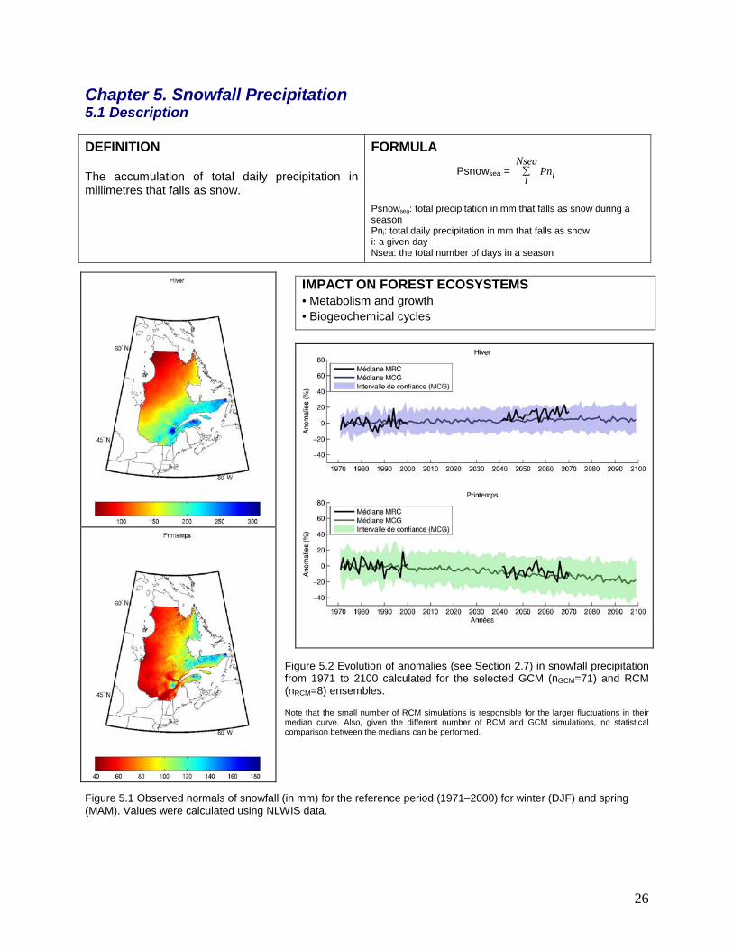
Chapter 5. Snowfall Precipitation 5.1 Description
DEFINITION The accumulation of total daily precipitation in millimetres that falls as snow.
FORMULA
Psnowsea = ∑Nsea
i iPn
Psnowsea: total precipitation in mm that falls as snow during a season Pni: total daily precipitation in mm that falls as snow i: a given day Nsea: the total number of days in a season
Figure 5.2 Evolution of anomalies (see Section 2.7) in snowfall precipitation from 1971 to 2100 calculated for the selected GCM (nGCM=71) and RCM (nRCM=8) ensembles. Note that the small number of RCM simulations is responsible for the larger fluctuations in their median curve. Also, given the different number of RCM and GCM simulations, no statistical comparison between the medians can be performed.
Figure 5.1 Observed normals of snowfall (in mm) for the reference period (1971–2000) for winter (DJF) and spring (MAM). Values were calculated using NLWIS data.
IMPACT ON FOREST ECOSYSTEMS • Metabolism and growth • Biogeochemical cycles

27
5.2 Impact on forest ecosystems Just as precipitation in liquid form is important during the growing season, snowfall precipitation is equally important for ecosystems in temperate and nordic climates. First, snow cover can have an important indirect impact on tree growth. Snow cover acts as an insulator, which controls soil temperatures and reduces soil freezing events (Decker et al. 2003; Campbell et al. 2005; Zhang et al. 2008; Auclair et al. 2010). This insulating effect is important for tree survival. Experimental studies have shown that removing snow throughout the winter season increases soil freezing, which causes major root damage (Robitaille et al. 1995; Weih and Karlsson 2002), partial canopy mortality (Boutin and Robitaille 1995; Robitaille et al. 1995), and a reduction in micro-organism communities in the ground (Sulkava and Huhta 2003). The survival of insect larvae in the soil may also be compromised by slight snow cover, which leads to lower temperatures and an increase in freeze/thaw events (Bale and Hayward 2010). Snowfall precipitation rates may also have a negative impact on soil water content in the spring, a crucial time for the start of plant growth. Snowfall precipitation can also be an important water source for the soil during the spring thaw. A lack of water during this period can slow the start of the growing season or reduce growth (Hoffer and Tardif 2009; Leblanc and Terrell 2009). What’s more, water content in the soil in the spring has an impact on the soil drought code index and, consequently, influences the risk of forest fires. A reduced snow cover can mean an
earlier start to the fire season and a longer season (Girardin et al 2006a, b). Snow cover and, in particular, its insulating power can also have a major impact on biogeochemical cycles, such as those of nitrogen and carbon. Impacts are complex and mixed, however. One direct impact of increased snow cover is better soil insulation, which leads to an increase in soil temperature (Monson et al. 2006; Morgner et al. 2010). This increase in soil temperature causes an increase in the respiration of the organisms living in the soil and therefore an increase in the carbon released by the system. Some studies show that a loss of snow cover in nordic environments, like the tundra, could transform these ecosystems into important sources of CO2 (Morgner et al. 2010). On the other hand, more clement temperatures can also transform snow into an ice cover, particularly if there has also been a buildup of liquid precipitation. In the short term, this ice can prevent carbon from leaving ecosystems (Morgner et al. 2010). Furthermore, reduced snow cover and increased soil freezing are also associated with disturbances in the nitrogen cycle, including losses through leaching in the form of nitrate (NO3
-) outside of the root zone (Boutin and Robitaille 1995; Robitaille et al. 1995; Brooks et al. 1998; Tierney et al. 2001). This leaching is partly explained by the fact that the melting snow cover increases the amount of water in the soil, which carries nitrates out of the root zone (Groffman et al. 2001; Joseph and Henry 2008). Moreover, root mortality, which is linked to soil freezing, reduces the amount of nitrate consumed by plants and increases the rate of nitrate lost from the root zone (Boutin and Robitaille 1995; Tierney et al. 2001).
28
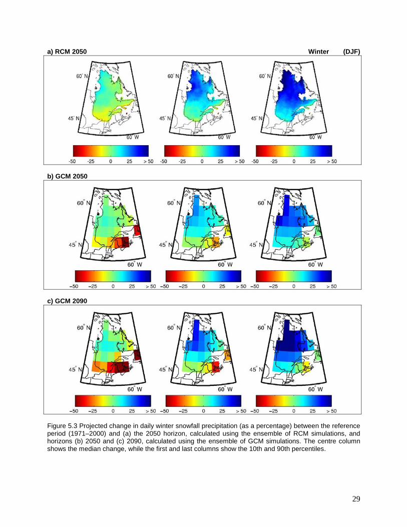
5.3 Snowfall precipitation results 5.3.1 Normals and anomalies Figure 5.1 shows the observed normals for snowfall precipitation (in mm) for the reference period (1971–2000) for winter (DJF) and spring (MAM). Figure 5.2 shows the evolution of anomalies (see Section 2.7) for snowfall precipitation from 1971 to 2100 calculated for the selected GCM (nGCM=71) and RCM (nRCM=8) ensembles. 5.3.2 Projected changes Note that projected changes are shown here as a percentage. Changes in mm can be consulted in Annex 3. Winter Figure 5.3 shows the changes of winter snowfall projected by the global and regional ensembles for the 2050 and 2090 horizons. For this season, both types of climate models project greater increases in snowfall in the centre and north of the province, with a very weak signal in the south. The RCM median varies from -10% to 10% in the south and from 15% to 50% in the north (Figure 5.3a). GCM and RCM values for the 2050 horizon are similar (Figure 5.3b). However, given the greater RCM resolution, maps produced with these models better display certain snowfall
precipitation gradients, such as the gradient around Hudson Bay, for example, which can arise from convection on Hudson Bay whenever the ice cover is incomplete. Differences between the 10th and 90th percentiles (inter-model variability) for the GCMs (for the 2050 and 2090 horizons) are greater than for the RCMs, particularly for southern Québec. Across the south of Québec, the GCM 10th percentiles project important reductions in snowfall precipitation. Spring Figure 5.4 shows a decrease in snowfall precipitation in the spring for central and southern Québec, while in the north, models project only very slight increases. For the 2050 horizon, the median projected by the RCMs and GCMs ranges from 0% to -25% for the centre of Québec (Figure 5.4 a, b). For the St. Lawrence Valley, further south, reductions reach -40%, while in the north increases range from 0% to 5%. For the 2090 horizon (Figure 5.4c), projected reductions for southern Québec are greater than those projected for 2050 by RCMs and GCMs, with a projected median of -25% to -50%. However, projected values for central and northern Québec in 2090 are more or less the same as the projected values for 2050 for these regions. Differences between the 10th and 90th percentiles are greater, however.
29
a) RCM 2050 Winter (DJF)
b) GCM 2050
c) GCM 2090
Figure 5.3 Projected change in daily winter snowfall precipitation (as a percentage) between the reference period (1971–2000) and (a) the 2050 horizon, calculated using the ensemble of RCM simulations, and horizons (b) 2050 and (c) 2090, calculated using the ensemble of GCM simulations. The centre column shows the median change, while the first and last columns show the 10th and 90th percentiles.

30
a) RCM 2050 Spring (MAM)
b) GCM 2050
c) GCM 2090
Figure 5.4 Projected change in daily spring snowfall precipitation (as a percentage) between the reference period (1971–2000) and (a) the 2050 horizon, calculated using the ensemble of RCM simulations, and horizons (b) 2050 and (c) 2090, calculated using the ensemble of GCM simulations. The centre column shows the median change, while the first and last columns show the 10th and 90th percentiles.

31
Chapter 6. Freeze/Thaw Events 6.1 Description
DEFINITION Days with a freeze/thaw event are days when the temperature oscillates above and below 0̊C in 24 hours. Specifically, a daily freeze/thaw event is observed when, within a 24-hour period, the minimum recorded temperature is below 0˚C and the maximum recorded temperature is above 0˚C.
FORMULA
Freeze/Thaw = )C0()C01
( °<°>∑= iTnand
Nsea
i iTx
Freeze/Thaw: the number of days with a freeze/thaw event during a season Txi: maximum daily temperature for a 24-hour period Tni: minimum daily temperature for a 24-hour period i: a given day Nsea: the total number of days in a season
Figure 6.2 Evolution of anomalies (see Section 2.7) in the number of freeze/thaw events from 1971 to 2100 calculated for the selected GCM (nGCM=71) and RCM (nRCM=8) ensembles. Note that the small number of RCM simulations is responsible for the larger fluctuations in their median curve. Also, given the different number of RCM and GCM simulations, no statistical comparison between the medians can be performed.
Figure 6.1 Observed normals of the number of freeze/thaw events (in days) for the reference period (1971–2000), for winter (DJF) and spring (MAM). Values were calculated using NLWIS data.
IMPACT ON FOREST ECOSYSTEMS • Metabolism and growth • Phenology • Distribution and migration • Biogeochemical cycles

32
6.2 Impact on forest ecosystems The impact of freeze/thaw events—defined here as when the air temperature is below and above 0°C on the same day—are no doubt the most complex and difficult to quantify. This is for a number of reasons: First, the impact of freeze/thaw events on plants is largely influenced by snow cover. Second, their impact on trees depends on the time of year (when trees are dormant or at the start of the growing season, for example). Third, the length of time the temperature spends above or below zero and the absolute temperature deviation with zero also have an effect. It is sometimes difficult to break down each of these factors in the literature. Freeze/thaw events have an important effect on tree robustness and mortality, even though this relationship can be difficult to quantify since freezing thresholds vary from one species to another. Nevertheless, the ability of trees to obtain and maintain an adequate level of resistance to freezing in late fall, winter, and spring is clearly vital. Moreover, a change in the frequency of freeze/thaw events seems to be the primary cause of a loss of resistance to cold temperatures for a number of species. For example, for black spruce, an increase in the frequency and intensity of freezing events is correlated to a decrease in photosynthesis (Gaumont-Guay et al. 2003). A number of studies carried out in Québec have shown the importance of freeze/thaw events and of a loss of tolerance to the cold for two species particularly susceptible to these phenomena: red spruce and yellow birch (Schaberg et al. 2000; Zhu et al. 2000, 2001, 2002; Lazarus et al. 2004; Bourque et al. 2005; Dumais and Prévost 2007). In fact, an increase in the frequency of winter thaw episodes and an increase in thaw length are closely correlated with a reduction in freezing tolerance for both red spruce and yellow birch (Lund and Livingston 1998; Schaberg et al. 2000; Zhu et al. 2000, 2002). Moreover, loss of cold resistance seems to be positively influenced by an increase in acid deposition from the atmosphere (Hamburg and Cogbill 1988; Schaberg et al. 2000; Zhu et al. 2002; Hawley et al. 2006). This phenomenon is so marked for red spruce that it is held largely responsible for the species’ population decline in northeastern America (Hamburg and Cogbill 1988; Schaberg et al. 2000; Hawley et al. 2006).
For red spruce, the loss of resistance to the cold is correlated with cell damage, needle mortality, and crown decline (Lazarus et al. 2004; Hawley et al. 2006; Dumais and Prévost 2007). A canopy loss then manifests itself through a reduction in carbon assimilation and reduced growth (Schaberg et al. 2000; Lazarus et al. 2004). For yellow birch, a loss of resistance to the cold leads to root and branch damage (Zhu et al. 2000, 2002). This damage then results in decreased growth and a significant loss in moisture absorption and root pressure. Given that root pressure in the spring must be sufficient to fill the embolisms caused by vessel cavitation over the winter, a loss of root pressure caused by freezing increases the mortality risk for the crown (Zhu et al. 2001, 2002). Finally, for red spruce and yellow birch, the timing of the freeze/thaw episodes also plays a determining role. The tolerance of red spruce to freezing develops slowly over the cold season, reaching its peak in the middle of winter (Dumais and Prévost 2007). An increase in freeze/thaw episodes before this period could therefore adversely affect the survival of red spruce. Moreover, red spruce is not profoundly dormant over winter compared to other conifers (Major et al. 2003). A shift in freeze/thaw events over the winter period could therefore also have an impact on red spruce’s survival. The species’ sensitivity to the cold and freezing seems to severely restrict its spatial distribution (Arris and Eagleson 1989). Yellow birch also loses its resistance to the cold very quickly with rising spring temperatures and the species would be particularly affected by an increase in freeze/thaw episodes in late winter and spring (Braathe 1995; Zhu et al. 2002). The resistance of yellow birch to the cold seems to be enough to maintain its spatial distribution in the current climate, but any loss of resistance due to changes in freeze/thaw events could mean reduced competitiveness (Zhu et al. 2002). Damage associated with freeze/thaw events is considerable for a number of other species. Sugar maple in particular, a very important commercial species in Québec, is strongly influenced by the intensity and timing of freeze/thaw events. First, damage due to soil freezing in winter can have negative impacts on tree health, sap run-off, total sap production, and the amount of sugar produced per tree in the spring (Robitaille et al. 1995). A recent study shows that Québec maple syrup production by tap tended to decrease between 1985 and 2006

33
(Duchesne et al. 2009). Annual production variations were largely explained by a climate prediction model. Using future climate scenarios, researchers forecast a reduction in maple syrup production of 15% to 20%. It has long been known that the maximum run-off for sugar maples in the spring is in sync with periods characterized by daytime temperature fluctuations around 0°C (Pothier 1995). Therefore, the expected reduction in syrup production by tap could be prevented if the sap run shifts in line with freeze/thaw events earlier in the spring and possibly in winter. As well as influencing vegetation directly, freeze/thaw cycles can have an indirect impact on the soil and on plants by influencing snow cover melt. First, a sufficiently long thaw period can be associated with longer melting events. These episodes are important since they increase the amount of water in the soil, which may then in turn bring about a bigger, faster transfer of nutrients like nitrate and other base cations (Lehrsch et al. 1991; Wang and Bettany 1993; Ferrick and Gatto 2005; Henry 2008). If these nutrients are not absorbed by the plants, they are leached out of the trees’ root zone (Robitaille et al. 1995; Weih and Karlsonn 2002; Campbell et al. 2005; Henry 2008). This phenomenon occurs in winter when trees are dormant and is often associated with an increase in nitrification and H+ cation production. These factors can significantly acidify the ground (Boutin and Robitaille 1995). Furthermore, this increased winter leaching, during a dormant period, implies that available nutrient concentrations will be weaker in the spring, a crucial growing period for trees (Lehrsch et al. 1991). Second, a partial melting of the snow due to above-zero temperatures can cause ice to form at the soil level (Fortin 2010). This ice can increase the thermal conductivity of the snow cover, which increases the risk of the soil freezing (Andrews 1996; Fortin 2010), changing the snow’s ecological role, and impacting gas and water exchanges between the soil, the snow, and the atmosphere (Tranter and Jones 2001; Larsen et al. 2002; Mikan et al. 2002; Campbell et al. 2005). For instance, although thawing and melting snow periods are often associated with an increase in the amount of water in the soil (e.g., Joseph and Henry 2008), ice formation may in fact have the opposite effect and reduce water infiltration into the soil (Zheng and Flerchinger 2001; Henry 2008). Finally, a total loss of snow in winter can bring about an increase in the number of freezing
events and lengthen the time the soil freezes. These increases can have important impacts on root survival and nutrient absorption, which in turn lead to losses in crown survival (Robitaille et al. 1995; Tierney et al. 2001; Auclair et al. 2010).

34
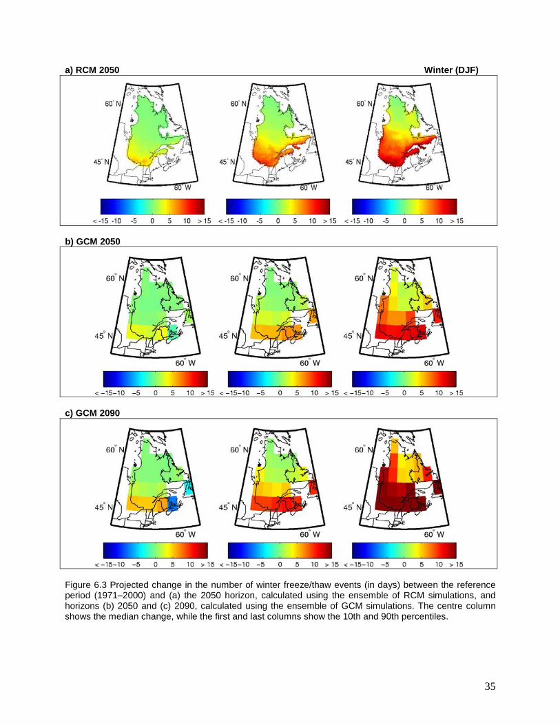
6.3 Freeze/thaw event results 6.3.1 Normals and anomalies Figure 6.1 shows the observed normals for the number of freeze/thaw events (in days) for the reference period (1971–2000), for winter (DJF) and spring (MAM). Figure 6.2 shows the evolution of anomalies (see Section 2.7) for the number of freeze/thaw events from 1971 to 2100 calculated for the selected GCM (nGCM=71) and RCM (nRCM=8) ensembles. 6.3.2. Projected changes Winter Figure 6.3 shows changes of the number of freeze/thaw events projected by the global and regional ensembles for the 2050 and 2090 horizons. All simulations project a slight increase in the number of freeze/thaw events for southern Québec, with no change for northern Québec. For the 2050 horizon, GCMs and RCMs project similar changes for central and northern Québec, with a median of 0 to 2 days. For southern Québec, however, RCMs (Figure 6.3a) project an increase of 5 to 13 days, slightly more than the projected GCM values (Figure 6.3b) of 5 to 8 days. GCM results for the 2090 horizon (Figure 6.3c) also show a north–south gradient with a 10–15 day increase in the number of events for southern Québec and a median of around 0 days for northern Québec. Spring All models project slight increases in the number of freeze/thaw events in the north, an almost constant number in the centre, and a decrease in the number of events in the south (Figure 6.4). Median changes for the 2050 horizon, projected by the RCMs and GCMs, are 3 to 5 days in the north, -1 to 3 days in the centre, and -5 to -10 days in the south (Figure 6.4 a, b). The 10th percentiles project important reductions in
southern Québec, while the 90th percentiles project a south–north gradient similar to those for the median values. Projected GCM values for the 2090 horizon (Figure 6.4c) are more or less the same as the values projected by RCMs and GCMs for the 2050 horizon, with fewer events in the south and a slight increase in the number of events in the north. There is, however, a greater difference between the 10th and 90th percentiles for the 2090 horizon. Annual Figure 6.5 shows the projected changes in the annual number of freeze/thaw events by the RCM and GCM ensembles for the 2050 and 2090 horizons. Projected changes for the number of freeze/thaw events are low: the projected RCM and GCM median for both horizons is -5 to -10 days. The 10th percentiles project a reduction in the number of events of approximately -10 days, while the 90th percentiles project no change (0 days). Changes shown on an annual basis provide better context for the projected winter increase (Figure 6.3) and the projected decrease in the number of spring events (Figure 6.4) in southern Québec. The increase in the number of winter events is due to a shift in the timing of events in the spring and fall in the current climate (Annex 3). This shift in the timing of events will be just as important, if not more, for vegetation as the change in the total number of freeze/thaw events. Atlas projections show that expected changes for freeze/thaw events are complex and deserve further exploration.
35
a) RCM 2050 Winter (DJF)
b) GCM 2050
c) GCM 2090
Figure 6.3 Projected change in the number of winter freeze/thaw events (in days) between the reference period (1971–2000) and (a) the 2050 horizon, calculated using the ensemble of RCM simulations, and horizons (b) 2050 and (c) 2090, calculated using the ensemble of GCM simulations. The centre column shows the median change, while the first and last columns show the 10th and 90th percentiles.

36
a) RCM 2050 Spring (MAM)
b) GCM 2050
c) GCM 2090
Figure 6.4 Projected change in the number of spring freeze/thaw events (in days) between the reference period (1971–2000) and (a) the 2050 horizon, calculated using the ensemble of RCM simulations, and horizons (b) 2050 and (c) 2090, calculated using the ensemble of GCM simulations. The centre column shows the median change, while the first and last columns show the 10th and 90th percentiles.

37
a) RCM 2050 Annual
b) GCM 2050
c) GCM 2090
Figure 6.5 Projected change in the number of annual freeze/thaw events between the reference period (1971–2000) and (a) the 2050 horizon, calculated using the ensemble of RCM simulations, and horizons (b) 2050 and (c) 2090, calculated using the ensemble of GCM simulations. The centre column shows the median change, while the first and last columns show the 10th and 90th percentiles.

38
Chapter 7. Growing Degree-Days 7.1 Description
DEFINITION The difference in degrees Celsius that separates the mean daily temperature from a base value of 5˚C. If the difference is equal to or less than 5˚C, the day has zero growing degree-days. Daily values for degree-days are accumulated on an annual basis. The base value of 5˚C was established according to plant growth and development. The basic assumption is that plants will grow only if the ambient temperature is greater than this minimum value. There is also presumed to be a quasi-linear relationship between growth increases and temperature increases or the accumulation of heat energy (Schenk 1996; Loehle 1998; Bonhomme 2000).
FORMULA
GDD = ∑=
−365
1)0,(
iTbaseiTmeaMax
GDD: total number of growing degree-days per year Tmeai: mean temperature of day i Tbase: base temperature of 5°C i: a given day
IMPACT ON FOREST ECOSYSTEMS
• Phenology • Species distribution and migration • Interaction between species
Figure 7.2 Evolution of anomalies (see Section 2.7) in the annual number of growing degree-days from 1971 to 2100 calculated for the selected GCM (nGCM=71) and RCM (nRCM=8) ensembles. Note that the small number of RCM simulations is responsible for the larger fluctuations in their median curve. Also, given the different number of RCM and GCM simulations, no statistical comparison between the medians can be performed.
Figure 7.1 Observed normals of the annual number of growing degree-days for the reference period (1971–2000). Values were calculated using NLWIS data.

39
7.2 Impact on forest ecosystems The greatest impact of a change in growing degree-days (GDD) is on species phenology. An accumulation of GDD beyond a certain threshold will advance the start of phenological events such as budbreak, leafing, and the flowering start or end date (Aber et al. 1995; Arora and Boer 2005). In agriculture, this correlation between GDD and plant development is particularly important since it means the steps in a harvest season can be estimated. Given that a GDD increase allows leaves to appear earlier on some deciduous species, it also means an earlier and a longer growing season (Bradley et al. 1999; Parmesan 2006). This earlier start can be significant for forest productivity. For example, Myneni et al. (1997) estimated that a difference of only a few days in the appearance of the canopy could cause a 20% increase in photosynthesis rates in a forest in northeastern North America. An individual species response to earlier phenological events could lead to changes in the composition of certain plant communities (Goldblum and Rigg 2005; Williams et al. 2007) and could disrupt a number of interactions between species (Parmesan 2006). These disturbances could, for instance, put the life cycles of herbivorous insects out of sync with the life cycles of their host plants or put the life cycles of certain plants out of sync with the life cycles of their pollinators (Harrington et al. 1999; Pearson and Dawson 2003; Visser and Both 2005). The importance of this synchrony between the springtime budding of broad-leaved trees and the hatching of herbivorous insects (e.g., Lepidoptera) has been shown in a number of species, such as poplars and oaks (Hunter and Elkinton 2000; Tikkanen and Julkunen-Tiitto 2003). The influence of degree-days on species distribution and migration is complex. The northern limit of species distribution can be restricted by a low number of GDD when, for example, the number of GDD is too small for certain basic biological functions to be completed, which also makes the species less competitive (Shafer et al. 2001). Northern migration and the appearance of a new species are therefore possible, provided GDD changes meet this species’ biological criteria and give it a competitive advantage over species already in
place that would be less well adapted to the new GDD (Shafer et al. 2001). On the other hand, GDD tend not to influence species distribution at the southern limit of distribution. 7.3 Growing degree-day results 7.3.1 Normals and anomalies Figure 7.1 shows the observed normals for the number of annual growing degree-days for the reference period (1971–2000). Figure 7.2 shows the evolution of anomalies (see Section 2.7) for the annual number of growing degree-days from 1971 to 2100 calculated for the selected GCM (nGCM=71) and RCM (nRCM=8) ensembles. 7.3.2 Projected changes Figure 7.3 shows the changes of the annual number of growing degree-days projected by the global and regional ensembles for the 2050 and 2090 horizons. There is a north–south latitudinal gradient with large increases in the south and no projected changes for central and northern Québec. In 2050, according to the RCMs, the median increase will vary by more than 600 degree-days in the south, while the projected change for the centre and the north is 0 degree-days (Figure 7.4a). Projected GCM median values (Figure 7.4b) are more or less the same, with the exception of Québec’s extreme south, where GCMs project a smaller increase in growing degree-days than the RCMs (400 versus 600 degree-days). Projected GCM values for the 2090 horizon (Figure 7.3c) are higher than for the 2050 horizon and range from 125 degree-days in the north to 600 degree-days in the south. The 90th percentile values for this horizon are also much higher than for the 2050 horizon.

40
a) RCM 2050
b) GCM 2050
c) GCM 2090
Figure 7.3 Projected change in the number of growing degree-days between the reference period (1971–2000) and (a) the 2050 horizon, calculated using the ensemble of RCM simulations, and horizons (b) 2050 and (c) 2090, calculated using the ensemble of GCM simulations. The centre column shows the median change, while the first and last columns show the 10th and 90th percentiles.
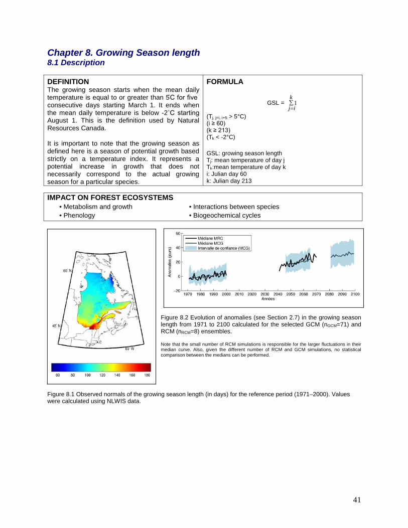
41
Chapter 8. Growing Season length 8.1 Description
DEFINITION The growing season starts when the mean daily temperature is equal to or greater than 5̊C for five consecutive days starting March 1. It ends when the mean daily temperature is below -2˚C starting August 1. This is the definition used by Natural Resources Canada. It is important to note that the growing season as defined here is a season of potential growth based strictly on a temperature index. It represents a potential increase in growth that does not necessarily correspond to the actual growing season for a particular species.
FORMULA
GSL = ∑=
k
ij1
(Tj, j=i, i+5 > 5°C) (i ≥ 60) (k ≥ 213) (Tk < -2°C) GSL: growing season length Tj: mean temperature of day j Tk:mean temperature of day k i: Julian day 60 k: Julian day 213
IMPACT ON FOREST ECOSYSTEMS
• Metabolism and growth • Interactions between species • Phenology • Biogeochemical cycles
Figure 8.2 Evolution of anomalies (see Section 2.7) in the growing season length from 1971 to 2100 calculated for the selected GCM (nGCM=71) and RCM (nRCM=8) ensembles. Note that the small number of RCM simulations is responsible for the larger fluctuations in their median curve. Also, given the different number of RCM and GCM simulations, no statistical comparison between the medians can be performed.
Figure 8.1 Observed normals of the growing season length (in days) for the reference period (1971–2000). Values were calculated using NLWIS data.
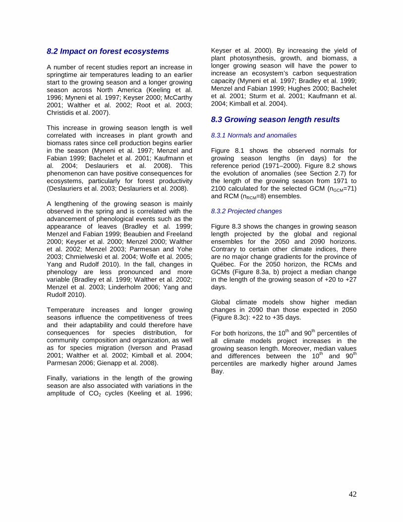
42
8.2 Impact on forest ecosystems A number of recent studies report an increase in springtime air temperatures leading to an earlier start to the growing season and a longer growing season across North America (Keeling et al. 1996; Myneni et al. 1997; Keyser 2000; McCarthy 2001; Walther et al. 2002; Root et al. 2003; Christidis et al. 2007). This increase in growing season length is well correlated with increases in plant growth and biomass rates since cell production begins earlier in the season (Myneni et al. 1997; Menzel and Fabian 1999; Bachelet et al. 2001; Kaufmann et al. 2004; Deslauriers et al. 2008). This phenomenon can have positive consequences for ecosystems, particularly for forest productivity (Deslauriers et al. 2003; Deslauriers et al. 2008). A lengthening of the growing season is mainly observed in the spring and is correlated with the advancement of phenological events such as the appearance of leaves (Bradley et al. 1999; Menzel and Fabian 1999; Beaubien and Freeland 2000; Keyser et al. 2000; Menzel 2000; Walther et al. 2002; Menzel 2003; Parmesan and Yohe 2003; Chmielweski et al. 2004; Wolfe et al. 2005; Yang and Rudolf 2010). In the fall, changes in phenology are less pronounced and more variable (Bradley et al. 1999; Walther et al. 2002; Menzel et al. 2003; Linderholm 2006; Yang and Rudolf 2010). Temperature increases and longer growing seasons influence the competitiveness of trees and their adaptability and could therefore have consequences for species distribution, for community composition and organization, as well as for species migration (Iverson and Prasad 2001; Walther et al. 2002; Kimball et al. 2004; Parmesan 2006; Gienapp et al. 2008). Finally, variations in the length of the growing season are also associated with variations in the amplitude of CO2 cycles (Keeling et al. 1996;
Keyser et al. 2000). By increasing the yield of plant photosynthesis, growth, and biomass, a longer growing season will have the power to increase an ecosystem’s carbon sequestration capacity (Myneni et al. 1997; Bradley et al. 1999; Menzel and Fabian 1999; Hughes 2000; Bachelet et al. 2001; Sturm et al. 2001; Kaufmann et al. 2004; Kimball et al. 2004). 8.3 Growing season length results 8.3.1 Normals and anomalies Figure 8.1 shows the observed normals for growing season lengths (in days) for the reference period (1971–2000). Figure 8.2 shows the evolution of anomalies (see Section 2.7) for the length of the growing season from 1971 to 2100 calculated for the selected GCM (nGCM=71) and RCM (nRCM=8) ensembles. 8.3.2 Projected changes Figure 8.3 shows the changes in growing season length projected by the global and regional ensembles for the 2050 and 2090 horizons. Contrary to certain other climate indices, there are no major change gradients for the province of Québec. For the 2050 horizon, the RCMs and GCMs (Figure 8.3a, b) project a median change in the length of the growing season of +20 to +27 days. Global climate models show higher median changes in 2090 than those expected in 2050 (Figure 8.3c): +22 to +35 days. For both horizons, the 10th and 90th percentiles of all climate models project increases in the growing season length. Moreover, median values and differences between the 10th and 90th percentiles are markedly higher around James Bay.
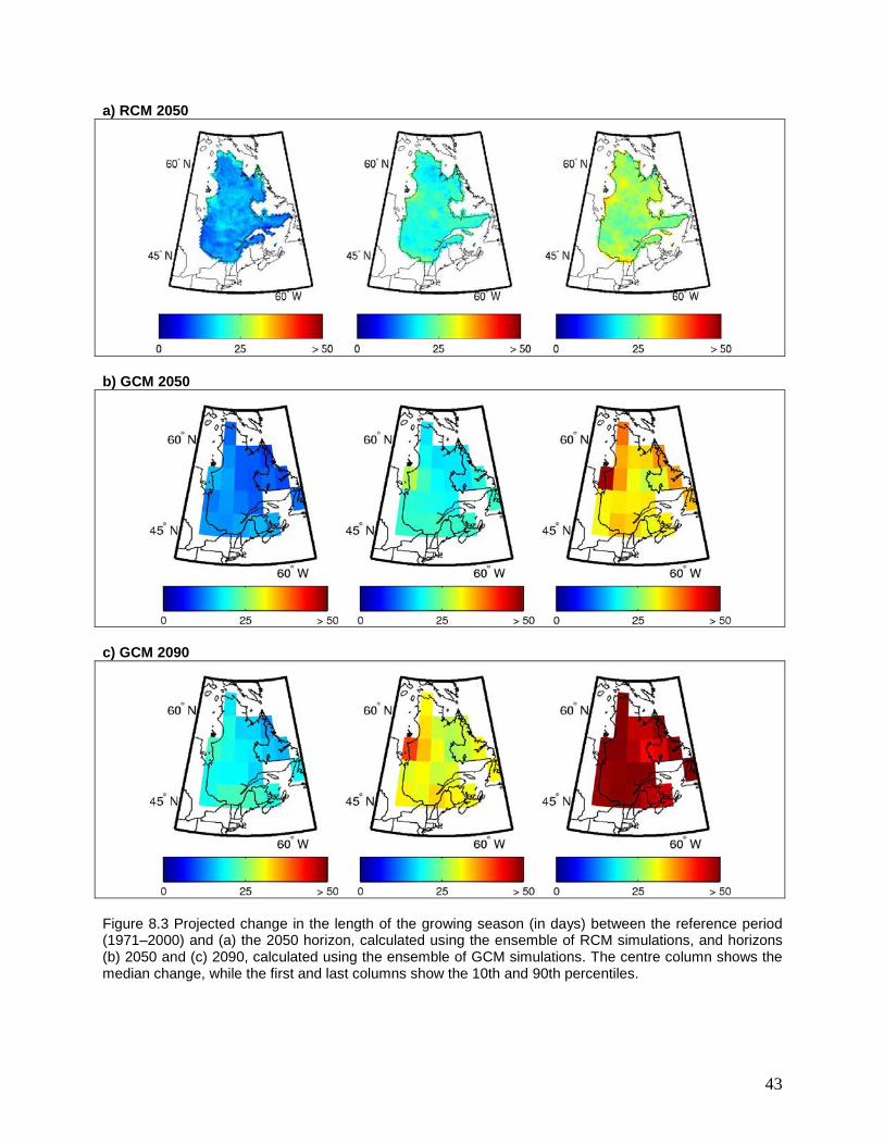
43
a) RCM 2050
b) GCM 2050
c) GCM 2090
Figure 8.3 Projected change in the length of the growing season (in days) between the reference period (1971–2000) and (a) the 2050 horizon, calculated using the ensemble of RCM simulations, and horizons (b) 2050 and (c) 2090, calculated using the ensemble of GCM simulations. The centre column shows the median change, while the first and last columns show the 10th and 90th percentiles.

44
Chapter 9. Canadian Drought Code 9.1 Description
DEFINITION The Canadian drought code is intended to be an empirical evaluation of the mean water content of forest soil. It is calculated based on combined daily temperatures and precipitation from April 1 to October 31, using the method proposed by Turner (1972).
FORMULA RP= (800/exp(CDC-1/400) +3.937ER
ER = 0.83P -1.27 D= 400In (800/RP)
PET= 0.36T + L CDC= D +0.5PET
CDC: Canadian drought code RP: water equivalent after rain d: a given day ER: effective precipitation P: daily precipitation above 2.80 mm D: current dryness PET: potential evapotranspiration L: length of day seasonal adjustment (See Turner 1972 for more information)
IMPACT ON FOREST ECOSYSTEMS
• Metabolism and growth • Frequency of natural disturbances
Figure 9.2 Evolution of anomalies (see Section 2.7) in the drought from 1971 to 2100 calculated for the selected GCM (nGCM=71) and RCM (nRCM=8) ensembles. Note that the small number of RCM simulations is responsible for the larger fluctuations in their median curve. Also, given the different number of RCM and GCM simulations, no statistical comparison between the medians can be performed.
Figure 9.1 Observed normals of the Canadian Drought Code for the reference period (1971–2000) from April to October. Values were calculated using NLWIS data.
45
9.2 Impact on forest ecosystems The drought index is a key component of the Forest Fire Weather Index (FWI). In Canada the FWI is used to estimate fire risks and behaviour. The index is based on a number of climate and non-climate variables: temperature, precipitation, humidity, solar radiation, burning agent, and wind (Van Wagner 1987; Flannigan and Harrington 1988). The FWI is made up of six components or indices, three of which are related to the water content of combustibles. Of the three indices related to the water content of combustibles, the drought code is probably the most often used to study the influence of climate on fires since it is good at estimating the impact of a change in evapotranspiration and precipitation on the reduction of water content in the ground. It is therefore correlated with a number of fire statistics, such as fire frequency and annual area burned variations (Larsen and MacDonald 1995; Girardin et al. 2004a, b; Ronnie et al. 2008; Girardin and Wotton 2009; Girardin et al. 2009). There are more fires and they spread more quickly when the climate is warm and dry and the drought code index is high (Johnson and Larsen 1991; Johnson 1992; Bessie and Johnson 1995; Skinner et al. 1999; Westerling et al. 2003). Moreover, a number of studies have shown a good correlation between the drought code and annual tree growth variations; this correlation is often used to reconstruct the past frequency of drought events (Bergeron and Archambault 1993; Tardif and Bergeron 1997; Girardin et al. 2006 a, b; Tardif and Conciatori 2006; Giradin and Mudalsee 2008). Growth rates of trees often decrease during periods when the drought code is high.
9.3 Canadian drought code results 9.3.1 Normals and anomalies Figure 9.1 shows the observed normals for the Canadian drought code for the reference period (1971–2000) from April to October. Figure 9.2 shows the evolution of anomalies (see Section 2.7) for the CDC from 1971 to 2100 calculated for the selected GCM (nGCM=71) and RCM (nRCM=8) ensembles. 9.3.2 Projected changes Figure 9.3 shows the changes in the Canadian drought code projected by the global and regional ensembles for the 2050 and 2090 horizons. The results show the mean change during the fire season, from April 1 to October 31. RCMs (Figure 9.3a) project a north–south gradient with a slight reduction in the drought code for the centre and the north, where the median is between -20 and 0 units, and a slight increase in the south with a projected median of 15 units. GCMs project a more uniform change across the province with a slight increase of 0 to 12 units for all of Québec (Figure 9.3b). For both models, the 10th percentiles project a reduction in the CDC for all of Québec. On the other hand, 90th percentile projections are more divided, with increases for all of Québec according to GCMs, but increases in the south and decreases in the north according to RCMs. Global climate model results for the 2090 horizon (Figure 9.3c) show changes comparable to GCM values for the 2050 horizon for central and northern Québec: an increase of 5 to 15 units. For the south, however, the median change is slightly greater, with a median of 10 to 22 units. Observed values for the CDC during the fire season can range from 0 (very low) to 400 or higher (extremely dry conditions). In Québec, the mean observed value for the fire season (April to October) was approximately 80 to 160 units (Figure 9.1), which gives Québec some of the lowest values in Canada. It should be noted that the change is not distributed equally within the fire season. The maximum projected changes by regional and global models are on the order of 25 units across Québec, which seems to indicate that changes will not be significant.
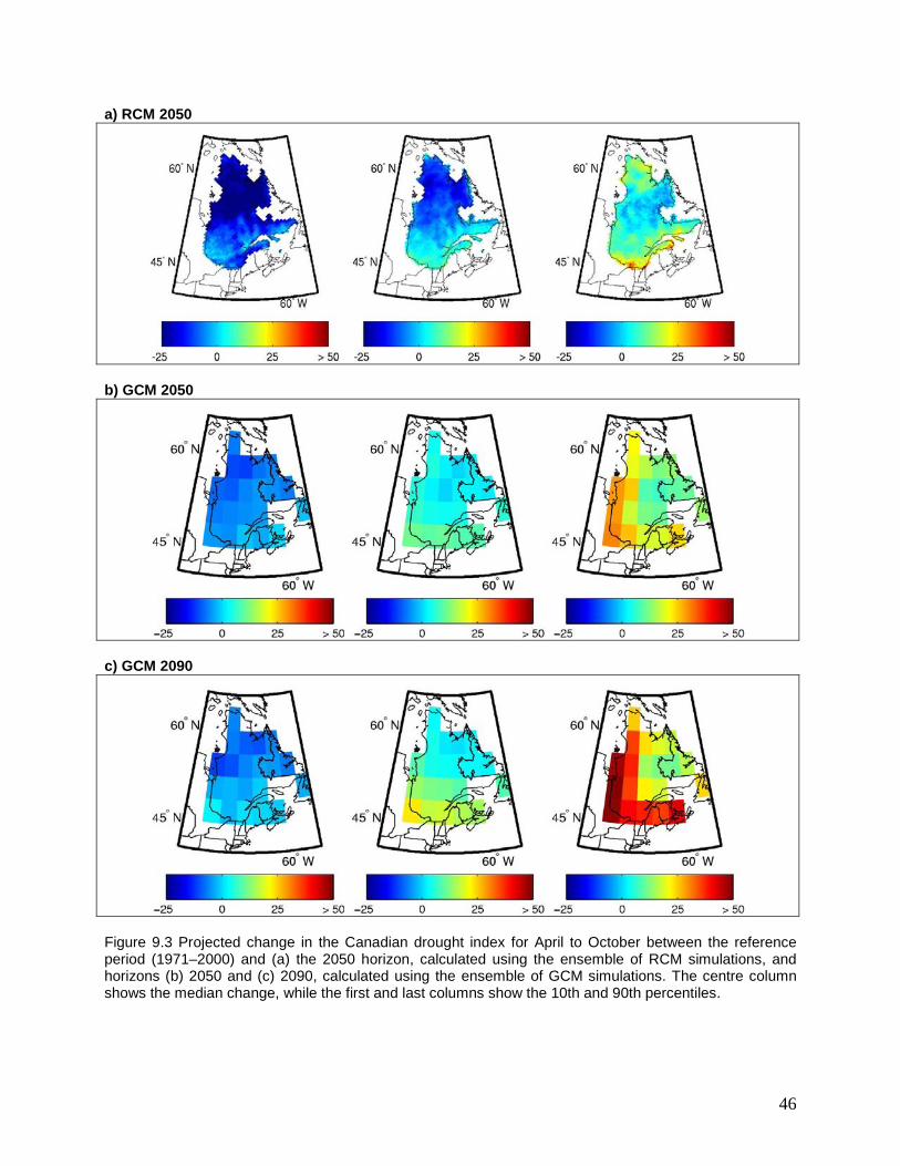
46
a) RCM 2050
b) GCM 2050
c) GCM 2090
Figure 9.3 Projected change in the Canadian drought index for April to October between the reference period (1971–2000) and (a) the 2050 horizon, calculated using the ensemble of RCM simulations, and horizons (b) 2050 and (c) 2090, calculated using the ensemble of GCM simulations. The centre column shows the median change, while the first and last columns show the 10th and 90th percentiles.

Conclusions The atlas provides an overview of the changes that can be expected for a number of climate variables and indices of interest for Québec’s forests. These changes are based on a large set of global climate simulations obtained from the PCMDI and a set of regional simulations produced by Ouranos available at the time of writing (fall 2010). Access to both information sources meant, on the one hand, that sources of uncertainty over climate projections could be better explored, and, on the one hand, that the spatial structure of regional change signals could be better represented. Atlas maps can be used to plan ecosystem projects in Québec forests and, more generally, in terrestrial ecosystems, notably concerning climate change adaptation. The main conclusions in terms of expected changes for the chosen variables for the 2050 and 2090 horizons are as follows: Mean temperature Models project a higher increase in mean temperature in northern Québec in winter, while in summer, the projected increase in mean temperature is greater in the south. Total precipitation In winter, models project a north–south gradient for Québec, with greater increases in total precipitation for the north. More precisely, the most marked increase is around Hudson Bay. In summer, projected increases in total precipitation in the north are low and models project no change in precipitation for southern Québec. Snowfall precipitation In winter, climate models project greater increases in snowfall for northern Québec over the south, where few changes are projected. In the spring, models project marked decreases in snowfall precipitation in the south and little change in the north. Freeze/thaw events In winter, models project a small increase in the number of freeze/thaw events in southern Québec, while the number of events in the centre and the north will remain stable. In the spring, the gradient is inversed, with a small increase in the number of freeze/thaw events in the north and a decrease in the number of events in the south. The projected change in the annual number of
events is very small. Closer analysis of this variable is required, in particular to determine the extent to which cycle intensities shift over time. Growing degree-days A change in the annual number of growing degree-days is projected only for southern Québec, with an increase in the number of degree-days. Models project no change for northern Québec. Growing season length Models project a longer growing season length across all of Québec. Unlike with certain other climate indices, there are no major change gradients across the province. Canadian Drought Code Models project very small increases in the drought code across Québec. Given that the observed mean values for Québec for the fire season (April to October) are among the lowest in Canada, the small projected increases appear to indicate that changes will not be significant.

57
References Aber JD, Ollinger SV, Federer CA, Reich PB, Goulden ML, Kicklighter DW, Melillo JM, Lathrop RG Jr. 1995. Predicting the effects of climate change on water yield and forest production in the northeastern United States. Clim. Res. 5: 207-222. Allen CD, Macalady AK, Chenchouni H, Bachelet D, McDowell N, Vennetier M, Kitzberger T, Rigling A, Breshears DD, Hogg EH, Gonzalez P, Fensham R, Zhang Z, Castro J, Demidova N, Lim J-H, Allard G, Running SW, Semerci A, Cobb N. 2010. A global overview of drought and heat-induced tree mortality reveals emerging climate change risks for forest. For. Ecol. Manag. 259: 660-684. Andrews CJ. 1996. How do plants survive ice? Annals Bot. 78: 529-536. Arora VK, Boer GJ. 2005. A parameterization of leaf phenology for the terrestrial ecosystem component of climate models. Glob. Change Bio. 11: 39-59. Arris LL, Eagleson PS. 1989. Evidence for a physiological basis for the boreal-deciduous forest ecotone in North America. Vegetatio 82: 55-58. Auclair AND, Heilman WE, Brinkman B. 2010. Predicting forest dieback in Maine, USA: a simple model based on soil frost and drought. Can. J. For. Res. 40: 687-702. Bachelet D, Neilson RP, Lenihan JT, Drapek RJ. 2001. Climate change effects on vegetation distribution and carbon budget in the United States. Ecosystems 4: 164-185. Bakkenes M, Alkemade JRM, Ihle F, Leemans R, Latour JB. 2002. Assessing the effects of forecasted climate change on the diversity and distribution of European higher plants for 2050. Glob. Change Bio. 8: 390-407. Bale JS, Hayward SAL. 2010. Insect overwintering in a changing climate. J. Exp. Bio. 213: 980-994. Battisti A, Stastny M, Netherer S, Robinet C, Schopf A, Roques A, Larsson S. 2005. Expansion of geographic range in the pine processionary moth caused by increased winter temperatures. Ecol. Appl. 15: 2084-2096. Beaubien EG, Freeland HJ. 2000. Spring phenology trends in Alberta, Canada: links to ocean temperature. Int. J. Biometeorol. 44: 53-59. Bergeron Y, Archambault S. 1993. Decreasing frequency of forest fires in the southern boreal zone of Québec and its relation to global warming since the end of the ‘Little Ice Age’. Holocene 3: 255-259.
Bergeron Y, Gauthier S, Kafka V, Lefort P, Lessieur D. 2001. Natural fire frequency for the eastern Canadian boreal forest: consequences for sustainable forestry. Can. J. For. Res. 31: 384-391. Bergeron Y, Cyr D, Drever CR, Flannigan M, Gauthier S, Kneeshaw D, Lauzon E, Leduc A, Le Goff H, Lesieur D, Logan K. 2006. Past, current, and future fire frequencies in Quebec’s commercial forests: implications for the cumulative effects of harvesting and fire on age-class structure and natural disturbance-based management. Can. J. For. Res. 36: 2737-2744. Bessie WC, Johnson EA. 1995. The relative importance of fuels and weather on fire behaviour in subalpine forests. Ecology 76: 747-762. Boisvenue C, Running SW. 2006. Impacts of climate change on natural forest productivity-evidence since the middle of the 20th century. Glob. Change Bio. 12: 868-882. Bonan GB, Shugart HH. 1989. Environmental factors and ecological processes in boreal forests. Annu. Rev. Ecol. Syst.20: 1-28. Bonhomme R. 2000. Bases and limits to using ‘degree.day’ units. Europ. J. Agronomy 13: 1-10. Bourque CP-A, Cox RM, Allen DJ, Arp PA, Meng F-R. 2005. Spatial extent of winter thaw events in eastern North America: historical weather records in relation to yellow birch decline. Glob. Change Bio. 11: 1477-1492. Boutin R, Robitaille G. 1995. Increased soil nitrate losses under mature sugar maple trees affected by experimentally induced deep frost. Can. J. For. Res. 25: 588-602. Braathe P. 1995. Birch dieback: caused by prolonged early spring thaws and subsequent frost. Norw. J. Agric. Sci. Suppl. 20. Bradley NL, Leopold AC, Ross J, Huffaker W. 1999. Phenological changes reflect climate change in Wisconsin. Proc. Natl. Acad. Sci. USA 96: 9701-9704. Briffa KR, Shishov VV, Melvin TM, Vaganov EA, Grudd H, Hantemirov RM, Eronen M, Naurzbaev MM. 2008. Trends in recent temperature and radial tree growth spanning 2000 years across northwest Eurasia. Phil Trans. R. Soc. B 363: 2269-2282. Brooks JR, Flanagan LB, Ehleringer JR. 1998. Responses of boreal conifers to climate fluctuations: indications from tree-ring widths and carbon isotope analyses. Can. J. For. Res. 28: 524-533. Campbell JL, Mitchell MJ, Groffman PM, Christenson LM, Hardy JP. 2005. Winter in northeastern North

58
America: a critical period for ecological processes. Front. Ecol. Environ. 3: 314-322. Canadell JG, Raupach MR. 2008. Managing forests for climate change mitigation. Science 320: 1456-1457. Caya D, Laprise. 1999. A semi-implicit semi-lagrangian regional climate model. Monthly Weather Review 127: 341-362 Chmielewski F-M, Müller A, Bruns E. 2004. Climate change and trends in phenology of fruit trees and field crops in Germany, 1961-2000. Agricul. Forest Meteorol. 121: 69-78. Christidis N, Stott PA, Brown S, Karoly DJ, Caesar J. 2007. Human contribution to the lengthening of the growing season during 1950-99. J. Climate 20: 5441-5454. Cleavitt NL, Fahey TJ, Groffman PM, Hardy JP, Henry KS, Driscoll CT. 2008. Effects of soil freezing on fine roots in a northern hardwood forest. Can. J. For. Res. 38: 82-91. Coulombe S, Bernier PY, Raulier F. 2009. Uncertainty in detecting climate change impact on the projected yield of black spruce (Picea mariana). For. Ecol. Manag. 259: 730-738. Danby RK, Hik DS. 2007. Responses of white spruce (Picea glauca) to experimental warming at a subarctic alpine treeline. Glob. C. Bio. 13: 437-451. Dang QL, Lieffers VJ. 1989. Climate and annual ring growth of black spruce in some Alberta peatlands. Can. J. Bot. 67: 1885-1889. Decker KLM, Wand D, Waite C, Scherbatskoy T. 2003. Snow removal and ambient air temperature effects on forest soil temperatures in Northern Vermont. Soil Sci. Soc. Am. J. 67: 1234-1243. Deslauriers A, Morin H, Urbinati C, Carrer M. 2003. Daily weather responses of balsam fir (Abies balsamea (L.) Mill.) stem radius increment from dendrometer analysis in the boreal forests of Québec (Canada). Trees 17: 477-484. Deslauriers A, Rossi S, Anfodillo T, Saracino A. 2008. Cambial phenology, wood formation and temperature thresholds in two contrasting years at high altitude in southern Italy. Tree Physiol. 28: 863-871. Duchesne L, Houle D, Côté M-A, Logan T. 2009. Modelling the effect of climate on maple syrup production in Québec, Canada. For. Ecol. Manage. 258: 2683-2689. Dumais D, Prévost M. 2007. Management for red spruce conservation in Québec: The importance of
some physiological and ecological characteristics-A review. For. Chron. 83: 378-392. Ferrick MG. Gatto LW. 2005. Quantifying the effect of a freeze-thaw cycle on soil erosion: laboratory experiments. Earth Surf. Proc. Land. 30: 1305-1326. Flannigan MD, Woodward FI. 1994. Red pine abundance: current climatic control and responses to future warming. Can. J. For. Res. 24: 1166-1175. Flannigan MD, Harrington JB. 1988. A study of the relation of meteorological variables to monthly provincial area burned by wildfire in Canada 1953-80. J. Appl. Meteorol. 27: 441-452. Flannigan M, Campbell I, Wotton M, Carcaillet C, Richard P, Bergeron Y. 2001. Future fire in Canada’s boreal forest: paleoecology results and general circulation model-regional climate model simulations. Can. J. For. Res. 31: 854-864. Flannigan MD, Logan KA, Amiro BD, Skinner WR, Stocks BJ. 2005. Future area burned in Canada. Clim. Change 72: 1-16. Foley JA, Costa MH, Delire C, Ramankutty N, Snyder P. 2003. Green surprise? How terrestrial ecosystems could affect earth’s climate. Front. Ecol. Environ. 1 : 38-44. Fortin G. 2010. Variabilité et fréquence des cycles de gel-dégel dans la région de Québec, 1977-2006. Can. Geog. 54: 196-208. Fritz HC. 2001. Tree rings and climate. Caldwell, New Jersey: Blackburn Press. 567 pp. Garfinkel HL, Brubaker LB. 1980. Modern climate-tree growth relationships and climate reconstruction in subarctic Alaska. Nature 286: 872-874. Gaumont-Guay D, Margolis BA, Bigras FJ, Raulier F. 2003. Characterizing the frost sensitivity of black spruce photosynthesis during cold acclimation. Tree Physiol. 23: 301-311 Gienapp P, Teplitsky C, Alho JS, Mills JA, Merilä J. 2008. Climate change and evolution: disentangling environmental and genetic responses. Mol. Ecol. 17: 167-178. Gillett NP, Weaver AJ, Zwiers FW, Flannigan M. 2004. Detecting the effect of climate change on Canadian forest fires. Geophys. Res. Letters 31: 1-4. Girardin MP, Wotton BM. 2009. Summer moisture and wildfire risks across Canada. J. appl. Meteorol. Climatology 48: 517-533.

59
Girardin MP, Mudelsee. 2008. Past and future changes in Canadian boreal wildfire activity. Ecol. Appl. 18: 391-406. Girardin MP, Ali AA, Carcaillet C, Mudelsee M, Drobyshev I, Hély C, Bergeron Y. 2009. Heterogeneous response of circumboreal wildfire risk to climate change since the early 1900s. Glob. Chang. Biol. 15: 2751-2769. Girardin MP, Tardif JC, Flannigan M, Bergeron Y. 2006a. Forest fire-conductive drought variability in the southern Canadian boreal forest and associated climatology inferred from tree rings. Can. Water Res. J. 31: 275-296. Girardin MP, Tardif J, Flannigan MD. 2006b. Temporal variability in area burned for the province of Ontario, Canada, during the past 200 years inferred from tree rings. J. Geophys. Res. 111: 1-10. Girardin MP, Tardif J, Flannigan MD, Bergeron Y. 2004a. Multicentury reconstruction of the Canadian Drought Code from eastern Canada and its relationship with paleoclimatic indices of atmospheric circulation. Climate Dyn. 23: 99-115. Girardin MP, Tardif J, Flannigan MD, Wotton BM, Bergeron Y. 2004b. Trends and periodicities in the Canadian Drought Code and their relationships with atmospheric circulation for the southern Canadian boreal forest. Can. J. For. Res. 34: 103-119. Glecker PJ, Taylor KE, Doutriaux C. 2008. Performance metrics for climate models. J. Geophys. Res. 113: D06104. Goldblum D, Rigg LS. 2005. Tree growth response to climate change at the deciduous-boreal forest ecotone, Ontario, Canada. Can. J. For. Res. 35: 2709-2718. Griesbauer HP, Green DS. 2010. Regional and ecological patterns in interior Douglas-fir climate-growth relationships in British Columbia, Canada. Can. J. For. Res. 40: 308-321. Groffman PM, Driscoll, CT, Fahey TJ, Hardy JP, Fitzhugh RD, Tierney GL. 2001. Colder soils in a warmer world: a snow manipulation study in a northern hardwood forest ecosystem. Biogeochem. 56: 135-150. Hamann A, Wang T. 2006. Potential effects of climate change on ecosystem and tree species distribution in British Columbia. Ecology 87: 2773-2786. Hamburg SP, Cogbill CV. 1988. Historical decline of red spruce populations and climatic warming. Nature 331: 428-431. Harrington R, Woiwod I, Sparks T. 1999. Climate change and trophic interactions. Trends Ecol Evol. 14: 146-150.
Harsch MA, Hulme PE, McGlone MS, Duncan RP. 2009. Are treelines advancing? A global meta-analysis of treeline responses to climate warming. Ecol. Letters 12: 1040-1049. Hawley GJ, Schaberg PG, Eagar C, Borer CH. 2006. Calcium addition at the Hubbard Brook Experimental Forest reduced winter injury to red spruce in a high-injury year. Can. J. For. Res. 36: 2544-2549. Henry HAL. 2008. Climate change and soil freezing dynamics: historical trends and projected changes. Clim. Change 87: 421-434. Hoffer M, Tardif JC. 2009. False rings in jack pine and black spruce trees from eastern Manitoba as indicators of dry summers. Can. J. For. Res. 39: 1722-1736. Huang J, Tardif JC, Bergeron Y, Denneler B, Berninger F, Girardin MP. 2010. Radial growth response of four dominant boreal tree species to climate along a latitudinal gradient in the eastern Canadian boreal forest. Glob. Change Bio. 16: 711-731. Hughes L. 2000. Biological consequences of global warming: is the signal already apparent? Trends Ecol. Evol. 15: 56-61. Hunter AF, Elkinton JS. 2000. Effects of synchrony with host plant on population of a spring-feeding lepidopteran. Ecology 81: 1248-1261. Iverson LR, Prasad AM. 2001. Potential changes in tree species richness and forest community types following climate change. Ecosystems 4: 186-199. Johnson EA. 1992. Fire and vegetation dynamics: studies from the North-American boreal forest. Cambridge Univ. Press, New York. Johnson EA, Larsen CPS. 1991. Climatically induced change in fire frequency in the southern Canadian Rockies. Ecology 72: 194-201. Joseph G, Henry HAL. 2008. Soil nitrogen leaching losses in response to freeze-thaw cycles and pulsed warming in a temperate old field. Soil Biol. Biochem. 40: 1947-1953. Kaufmann RK, D’Arrigo RD, Laskowski C, Myneni RB, Zhou L, Davi NK. 2004. The effect of growing season and summer greenness on northern forests. Geophys. Res. Lett. 31: 1-4. Keeling CD, Chin JFS, Whorf TP. 1996. Increased activity of northern vegetation inferred from atmospheric CO2 measurements. Nature 382: 146-149. Keyser AR, Kimball JS, Nemani S, Running SW. 2000. Simulating the effects of climate change on the carbon

60
balance of North American high-latitude forests. Glob. Chang. Biol. 6: 185-195. Kimball JS, McDonald KC, Running SW, Frolking SE. 2004. Satellite radar remote sensing of seasonal growing seasons for boreal and subalpine evergreen forests. Remote Sensing of Environment 90: 243-258. Koerner C. 2000. Bioshpere responses to CO2 enrichment. Ecol. App. 10: 1590-1619. Kullman L. 2001. 20th century climate warming and tree-limit rise in the southern Scandes of Sweden. Ambio 30: 72-80. Kurtz WA, Stinson G, Rampley G. 2008. Could increased boreal forest ecosystem productivity offset carbon losses from increases disturbances? Phil. Trans. R. Soc. B 363: 2259-2268. Larsen CPS, MacDonald GM. 1995. Relations between tree-rind widths, climate, and annual area burned in the boreal forest of Alberta. Can. J. For. Res. 25: 1746-1755. Larsen KS, Jonasson S, Michelsen A. 2002. Repeated freeze-thaw cycles and their effects on biological processes in two arctic ecosystem types. Appl. Soil Ecol. 21: 187-195. Lazarus BE, Schaberg PG, DeHayes DH, Hawley. 2004. Severe red spruce winter injury in 2003 creates unusual ecological event in the northeastern United States. Can. J. For. Res. 34: 1784-1788. Leblanc DC, Terrell MA. 2009. Radial growth response of white oak to climate in eastern North America. Can. J. For. Res. 39: 2180-2192. Lehrsch GA, Sojka RE, Carter DL, Jolley PM. 1991. Freezing effects on aggregate stability affected by texture, mineralogy, and organic matter. Soil Sc. Soc. Am. J. 55: 1401-1406. Lescop-Sinclair K, Payette S. 1995. Recent advance of the Arctic treeline along the eastern coast of Hudson Bay. J. Ecol. 83: 929-936. Linderholm HW. 2006. Growing season changes in the last century. Agric. Forest Meteorol. 137: 1-14. Lindner M, Maroschek M, Netherer S, Kremer A, Barbati A, Garcia-Gonzalo J, Seidl R, Delzon S, Corona P, Kolström, Lexer MJ, Marchetti M. 2010. Climate change impacts, adaptive capacity, and vulnerability of European forest ecosystems. For. Ecol. Manag. 259: 698-709. Lloyd AH. 2005. Ecological histories from Alaskan tree lines provide insight into future change. Ecology 86: 1687-1695.
Loehle C. 1998. Height growth rate tradeoffs determine northern and southern range limits for trees. J. Biogeogr. 25: 735-742. Logan T, Bourgages L, Huard D, Chaumont D. 2010. Sélection objective des scénarios climatiques pour l’analyse d’impacts et l’adaptation aux changements climatiques. Affiche présentée au 4e Symposium scientifique d’Ouranos, Novembre 2010. Logan JA, Réginère J, Powell JA. 2003. Assessing the impacts of global warming on forest pest dynamics. Front. Ecol. Environ. 1: 130-137. Lund A, Livingston WH. 1998. Freezing cycles enhance winter injury in Picea rubens. Tree Physiol. 19: 65-69. MacDonald GM, Kremenetski KV, Beilman DW. 2008. Climate change and the northern Russian treeline zone. Phil Trans. R. Soc. B 363: 2283-2299. MacDonal GM, et al. 2000. Holocene tree line history and climate change across northern Eurasia. Quat. Res. 53: 302-311. Major JE, Barsi DC, Mosseler A, Campbell M, Rajora OP. 2003. Light-energy processing and freezing-tolerance traits in red spruce and black spruce: species and seed-source variation. Tree Physiol. 23: 685-694. McCarty JP. 2001. Ecological consequences of recent climate change. Conserv. Bio. 15: 320-331. McKenney DW, Pedlar JH, Lawrence K, Campbell K, Hutchinson MF. 2007. Potential impacts of climate change on the distribution of North American trees. Bioscience 57: 939-948. Meehl GA, Covey C, Delworth T, Latif M, McAyaney B, Mitchell JFB, Stouffer RJ. Taylor KE. 2007. The WCRP CMIP3 multimodel dataset-A new era in climate change research. Bull. Am. Meteor. Soc. 88: 1383-1394. Menzel A. 2000. Trends in phenological phases in Europe between 1951 and 1996. Int. J. Biometeorol. 44: 76-81. Menzel A. 2003. Plant phonological anomalies in Germany and their relation to air temperature and NAO. Clim. Change 57: 243-263. Menzel A, Fabian P. 1999. Growing season extended in Europe. Nature 397: 659. Menzel A, Jakobi G, Ahas R, Scheifinger H, Estrella N. 2003. Variations of the climatological growing season (1951-2000) in Germany compared with other countries. Int. J. Climatol. 23: 793-812.

61
Mikan C, Schimel J, Doyle A. 2002. Temperature controls of microbial respiration above and below freezing in Arctic tundra soils. Soil Biol. Biochem. 34: 1785-1795 Millar CI, Stephenson NL, Stephens SL. 2007. Climate change and forests of the future: managing in the face of uncertainty. Ecol. Appl. 17: 2145-2151. Monson RK, Lipson DL, Burns SP, Turnipseed AA, Delany AC, Williams MW, Schmidt SK. 2006. Winter forest soil respiration controlled by climate and microbial community composition. Nature 439:711-714. Morgner E, Elberling B, Strebel D, Cooper EJ. 2010. The importance of winter in annual ecosystem respiration in the High Arctic: effects of snow depth in two vegetation types. Polar Res. 29: 58-74. Murphy JM, Sexton DMH, Barnett DN, Jones GS, Webb MJ, Collins M, Stainforth DA. 2004. Quantification of modelling uncertainties in a large ensemble of climate change simulations. Nature 430: 768-772. Music B, Caya D. 2007. Evaluation of the hydrological cycle over the Mississippi River basin as simulated by the Canadian Regional Climate Model (CRCM). J. Hydrometeo. 8: 969-988. Myneni RB, Keeling CD, Tucker CJ, Asrar G, Nemani RR. 1997. Increased plant growth in the northern high latitudes from 1981 to 1991. Nature 386: 698-702. Nakicenovic N, Alcamo J, Davis G, deVries B, Fenhann J, Gaffin S, Gregory K, Grübler A, Jung TY, Kram T, La Rovere EL, Michaelis L, Mori S, Morita T, Pepper W, Pitcher H, Price L, Raihi K, Roehrl A, Rogner H-H, Sankovski A, Schlesinger M, Shukla P, Smith S, Swart R, van Roojjen S, Victor N, Dadi Z. 2000. Emissions scenarios. Special report by Working group III of the Intergovernmental Panel on Climate Change. Cambridge University Press, 599pp. Parmesan C. 2006. Ecological and evolutionary responses to recent climate change. Annu. Rev. Ecol. Evol. Syst. 37: 637-669. Parmesan C, Yohe G. 2003. A globally coherent fingerprint of climate change impacts across natural systems. Nature 421: 37-42. Payette, S. 2007. Contrasted dynamics of northern Labrador tree lines caused by climate change and migrational lag. Ecology 88: 770-780. Pearson RG, Dawson TP. 2003. Predicting the impacts of climate change on the distribution of species: are bioclimate envelope models useful? Glob. Ecol. Biogeogr. 12: 361-371.
Pothier D. 1995. Effets des coupes d’éclaircie et des variations climatiques inter-annuelles sur la production et la teneur en sucre de la sève d’une érablière. Can. J. For. Res. 25: 1815-1820. Robitaille G, Boutin R, Lachance D. 1995. Effects of soil freezing stress on sap flow and sugar content of mature sugar maples (Acer saccharum). Can. J. For. Res. 25: 577-587. Ronnie DC, Drever MC, Messier C, Bergeron Y, Flannigan M. 2008. Fire and the relative roles of weather, climate and landscape characteristics in the Great Lakes-St. Lawrence forest of Canada. J. Veg. Sci. 19: 57-66. Root TL, Price JT, Hall KR, Schneider SH, Rosenzweig C, Pounds JA. 2003. Fingerprints of global warming on wild animals and plants. Nature 421: 57-60. Schaberg PG, DeHayes DH, Hawley GJ, Strimbeck GR, Cummin JR, Murakami PF, Borer CH. 2000. Acid mist and soil Ca and Al alter the mineral nutrition and physiology of red spruce. Tree Physiol. 20: 73-85. Schenk HJ. 1996. Modeling the effects of temperature on growth and persistence of tree species: a critical review of tree population models. Ecol. Model. 92: 1-32. Shafer SL, Bartlein PJ, Thompson RS. 2001. Potential changes in the distributions of Western North American tree and shrub taxa under future climate scenarios. Ecosystems 4: 200-215. Skinner WR, Flannigan M, Stocks BJ, Martell DL, Wotton BM, Todd JB, Mason JA, Logan KA, Bosch EM. 1999. A 500hPa synoptic wildland climatology for large Canadian Forest Fires, 1959-1996. Theor. Appl. Climatol. 71: 157-169. Sulkava P, Huhta V. 2003. Effects of hard frost and freeze-thaw cycles on decomposer communities and N mineralisation in boreal forest soil. Appl. Soil Ecol. 22: 225-239 Stocks BJ, Frosberg MA, Lynham TJ, Mearns L, Wotton BM, Yang Q, Jin J-Z, Lawrence K, Hartley GR, Mason JA, McKenney DW. 1998. Climate change and forest fire potential in Russian and Canadian boreal forests. Clim. Change 38: 1-13. Stocks BJ, Mason JA, Todd JB, Bosch EM, Wotton BM, Amiro BD, Flannigan MD, Hirsch KG, Logan KA, Martell DL, Skinner WR. 2003. J. Geophys. Res. 108: DI 1849. Sturm M, Racine C, Tape K. 2001. Increasing shrub abundance in the Arctic. Nature 411: 546-547.

62
Tardif, J. and Bergeron, Y. 1997. Ice-flood history reconstructed with tree-rings from the southern boreal forest limit, western Quebec. Holocene 7: 291-300. Can. J. For. Res. 36: 2317-2330. Tardif JC, Conciatori F. 2006. Influence of climate on tree rings and vessel features in red oak and white oak growing near their northern distribution limit, southwester Quebec, Canada. Can. J. For. Res. 36: 2317-2330. Thuiller W, Lavorel S, Araújo. 2005. Niche properties and geographical extent as predictors of species sensitivity to climate change. Glob. Ecol. Biogeogr. 14: 347-357. Tierney GL, Fahey TL, Groffman PM, Hardy JP, Fitzhugh RD, Driscoll CT. 2001. Soil freezing alters fine root dynamics in a northern hardwood forest. Biogeochem. 56: 175-190. Tikkanen O-P, Julkunen-Titto R. 2003. Phenological variation as protection against defoliating insects: the case of Quercus robur and Operophtera brumata. Oecologia 136: 244-251. Tranter M, Jones HG. 2001. The chemistry of snow: Processes and nutrient cycling. In Snow Ecology: An interdisciplinary examination of snow-covered ecosystems. Eds. Jones HG, Pomeroy JW, Walker DA, Homan RW. Cambridge: Cambridge University Press, 127-167. Turner JA. 1972. The drought code component of the Canadian Forest Fire Behaviour System. Environment Canada, Canadian Forest Service Publication 1316, Ottawa, ON, Canada, 14pp. Van Wagner CE. 1987. Development and structure of the Canadian Forest Fire Weather Index System. Forestry Tech. Rep. 35. Canadian Forest Service, Ottawa, ON, Canada, 37pp. Visser ME, Both C. 2005. Shifts in phenology due to global climate change: the need for a yardstick. Proc. R. Soc. B. 272: 2561-2569. Walther GR, Post E, Convery P, Menzel A, Parmesan C, Beebee TJC, Fromentin J-M, Hoegh-Guldberg O, Bairlein F. 2002. Ecological responses to recent climate change. Nature 416: 389-395. Wang FL, Bettany JR. 1993. Influence of freeze-thaw and flooding on the loss of soluble organic-carbon and carbon-dioxide from soil. J. Environ. Qual. 22: 709-714. Wang L, Payette S, Bégin Y. 2002. Relationships between anatomical and densitometric characteristics of black spruce and summer temperature at tree line in northern Quebec. Can. J. For. Res. 32: 477-486.
Wang T, Hamann A, Spittlehouse DL, Aitken SN. 2006. Development of scale-free climate data for western Canada for use in resource management. Int. J. Climatol. 26: 383-397. Weber MG, Flannigan M. 1997. Canadian boreal forest ecosystem structure and function in a changing climate: impact on fire regime. Environ. Rev. 5: 145-166. Weih M, Karlsson PS. 2002. Low winter soil temperature affects summertime nutrient uptake capacity and growth rate of mountain birch seedlings in the subarctic, Swedish Iapland. Arct. Antarct. Alp. Res. 34: 434-439. Westerling AL, Gershunov A, Brown TJ, Cayan DR, Dettinger MD. 2003. Climate and wildfire in the Western United States. Bull. Am. Meteorol. Soc. 84: 595-604. Westerling AL, Hidalgo HG, Cayan DR, Swetnam TW. 2006. Warming and earlier spring increase western U.S. forest wildfire activity. Science 313: 940-943. Williams JW, Jackson ST, Kutzbach JE. 2007. Projected distributions of novel and disappearing climates by 2100 AD. Proc. Nat. Ac. Sci. 104: 5738-5742. Wilmking M, Juday GP, Barber VA, Zald HSJ. 2004. Recent climate warming forces contrasting growth responses of white spruce at treeline in Alaska through temperature thresholds. Glob. C. Bio. 10: 1724-1736. Wolfe DW, Schwartz MD, Lakso AN, Otsuki Y, Pool RM, Shaulis NJ. 2005. Climate change and shifts in spring phenology of three horticultural woody perennials in northeastern USA. Int. J. Biometeorol. 49: 303-309 Woods A, Coates KD, Hamman A. 2005. Is an unprecedented Dothistroma needle blight epidemic related to climate change? Bioscience 55:761-769. Woodward FI, Lomas MR, Kelly CK. 2004. Global climate and the distribution of plant biomes. Phil. Trans. R. Soc. Lon. B 359: 1465-1476. Wotton BM, Flannigan MD. 1993. Length of the fire season in a changing climate. For. Chron. 69: 187-192. Wotton BM, Martell DL, Logan KA. 2003. Climate change and people-caused forest fire occurrence in Ontario. Climate Change 60: 275-295. Yang LH, Rudolf VHM. 2010. Phenology, ontogeny and the effects of climate change on the timing of species interactions. Ecology Letters 13: 1-10.

63
Zhang Y, Wang S, Barr AG, Black TA. 2008. Impact of snow cover on soil temperature and its simulation in a boreal aspen forest. Cold Reg. Sci. Technol. 52: 355-370. Zheng XQ, Flerchinger GN. 2001. Infiltration into freezing and thawing soil under different field treatments. J. Irrig. Drain. 127: 176-182. Zhu XB, Cox RM, Arp PA. 2000. Effects of xylem cavitation and freezing injury on dieback of yellow birch
(Betual alleghaniensis) in relation to a simulated winter thaw. Tree Physiol. 20: 541-547. Zhu XB, Cox RM, Meng F-R, Arp PA. 2001. Responses of xylem cavitation, freezing injury and shoot dieback to a simulated winter thaw in yellow birch seedlings growing in different nursery culture regimes. For. Ecol. Manage, 145: 243-253. Zhu, XB, Cox RM, Bourque C-PA, Arp PA. 2002. Thaw effects on cold-hardiness parameters in yellow birch. Can. J. Bot. 80: 390-39.

ANNEX 1-Climate normals
64
Annex 1 Maps of observed climate normals: all seasons Mean temperature a) DJF b) MAM
c) JJA d) SON
Figure A1.1 Observed normals of mean temperatures (in ̊ C) for the reference period (1971 –2000) for (a) winter (DJF), (b) spring (MAM), (c) summer (JJA) and (d) fall (SON). Values were calculated using NLWIS data.
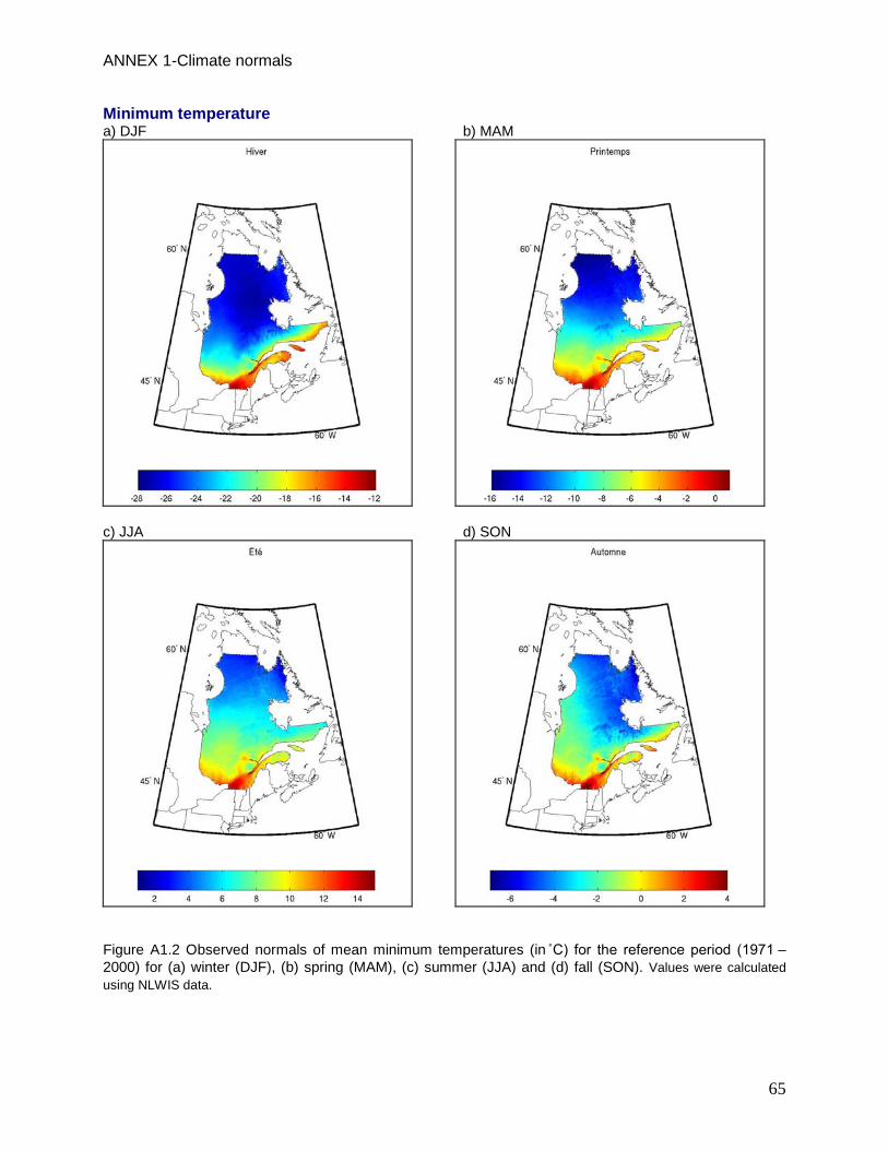
ANNEX 1-Climate normals
65
Minimum temperature a) DJF b) MAM
c) JJA d) SON
Figure A1.2 Observed normals of mean minimum temperatures (in ̊ C) for the reference period (1971 –2000) for (a) winter (DJF), (b) spring (MAM), (c) summer (JJA) and (d) fall (SON). Values were calculated using NLWIS data.

ANNEX 1-Climate normals
66
Maximum temperature a) DJF b) MAM
c) JJA d) SON
Figure A1.3 Observed normals of mean maximum temperatures (in ̊C) for the reference period (1971 –2000) for (a) winter (DJF), (b) spring (MAM), (c) summer (JJA) and (d) fall (SON). Values were calculated using NLWIS data.
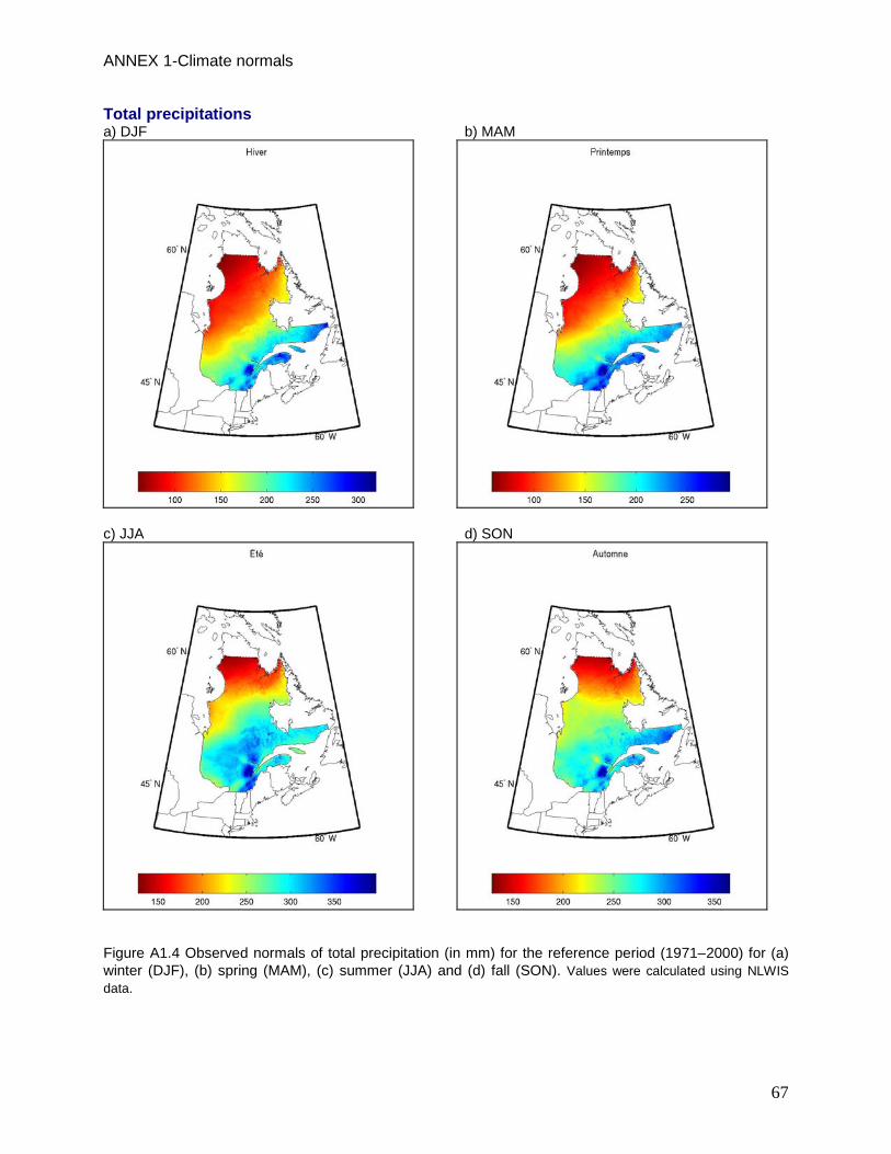
ANNEX 1-Climate normals
67
Total precipitations a) DJF b) MAM
c) JJA d) SON
Figure A1.4 Observed normals of total precipitation (in mm) for the reference period (1971–2000) for (a) winter (DJF), (b) spring (MAM), (c) summer (JJA) and (d) fall (SON). Values were calculated using NLWIS data.

ANNEX 1-Climate normals
68
Snowfall precipitation a) DJF b) MAM
c) SON
Figure A1.5 Observed normals of snowfall (in mm) for the reference period (1971–2000) for (a) winter (DJF), (b) spring (MAM) and (c) fall (SON). Values were calculated using NLWIS data.
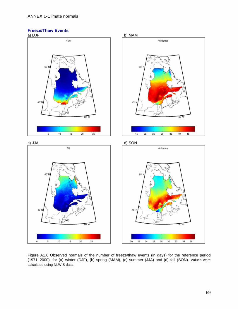
ANNEX 1-Climate normals
69
Freeze/Thaw Events a) DJF b) MAM
c) JJA d) SON
Figure A1.6 Observed normals of the number of freeze/thaw events (in days) for the reference period (1971–2000), for (a) winter (DJF), (b) spring (MAM), (c) summer (JJA) and (d) fall (SON). Values were calculated using NLWIS data.

ANNEX 1-Climate normals
70
Growing Degree-Days
Figure A1.7 Observed normals of the annual number of growing degree-days for the reference period (1971–2000). Values were calculated using NLWIS data.

ANNEX 1-Climate normals
71
Growing Season length
Figure A1.8 Observed normals of the growing season length (in days) for the reference period (1971–2000). Values were calculated using NLWIS data.

ANNEX 1-Climate normals
72
Canadian Drought Code
Figure A1.9 Observed normals of the Canadian Drought Code for the reference period (1971–2000) from April to October. Values were calculated using NLWIS data.

ANNEX 2 Evolution of anomalies
73
Annex 2 Evolution of anomalies: all seasons Mean temperature
Figure A2.1 Evolution of anomalies for mean temperature from 1971 to 2100 calculated for the selected GCM (nGCM=71) and RCM (nRCM=8) ensembles.

ANNEX 2 Evolution of anomalies
74
Minimum temperature
Figure A2.2 Evolution of anomalies for minimum temperature from 1971 to 2100 calculated for the selected GCM (nGCM=71) and RCM (nRCM=8) ensembles.
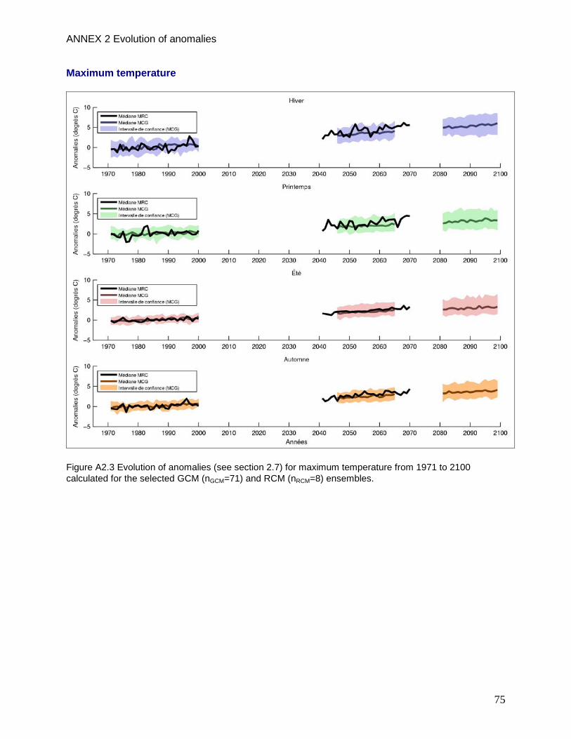
ANNEX 2 Evolution of anomalies
75
Maximum temperature
Figure A2.3 Evolution of anomalies (see section 2.7) for maximum temperature from 1971 to 2100 calculated for the selected GCM (nGCM=71) and RCM (nRCM=8) ensembles.
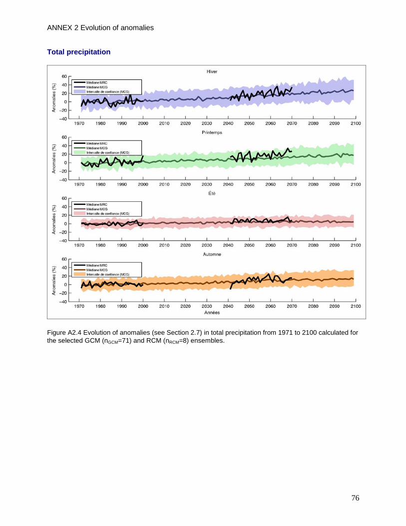
ANNEX 2 Evolution of anomalies
76
Total precipitation
Figure A2.4 Evolution of anomalies (see Section 2.7) in total precipitation from 1971 to 2100 calculated for the selected GCM (nGCM=71) and RCM (nRCM=8) ensembles.

ANNEX 2 Evolution of anomalies
77
Snowfall precipitation
Figure A2.5 Evolution of anomalies (see Section 2.7) in snowfall precipitation from 1971 to 2100 calculated for the selected GCM (nGCM=71) and RCM (nRCM=8) ensembles.

ANNEX 2 Evolution of anomalies
78
Freeze/thaw events
Figure A2.6 Evolution of anomalies (see Section 2.7) in the number of freeze/thaw events from 1971 to 2100 calculated for the selected GCM (nGCM=71) and RCM (nRCM=8) ensembles.

ANNEX 2 Evolution of anomalies
79
Growing Degree-Days
Figure A2.7 Evolution of anomalies (see Section 2.7) in the annual number of growing degree-days from 1971 to 2100 calculated for the selected GCM (nGCM=71) and RCM (nRCM=8) ensembles.

ANNEX 2 Evolution of anomalies
80
Growing Season length
Figure A2.8 Evolution of anomalies (see Section 2.7) in the growing season length from 1971 to 2100 calculated for the selected GCM (nGCM=71) and RCM (nRCM=8) ensembles

ANNEX 2 Evolution of anomalies
81
Canadian Drought Code
Figure A2.9 Evolution of anomalies (see Section 2.7) in the drought index from 1971 to 2100 calculated for the selected GCM (nGCM=71) and RCM (nRCM=8) ensembles.

ANNEX 3 – Maps of projected changes
82
Annex 3 Maps of projected changes: all seasons Mean temperature a) RCM 2050 Winter -DJF
b) GCM 2050
c) GCM 2090
Figure A3.1. Projected change in mean daily winter temperature (in °C) between the reference period (1971–2000) and (a) the 2050 horizon, calculated using the ensemble of RCM simulations, and horizons (b) 2050 and (c) 2090, calculated using the ensemble of GCM simulations. The centre column shows the median change, while the first and last columns show the 10th and 90th percentiles.
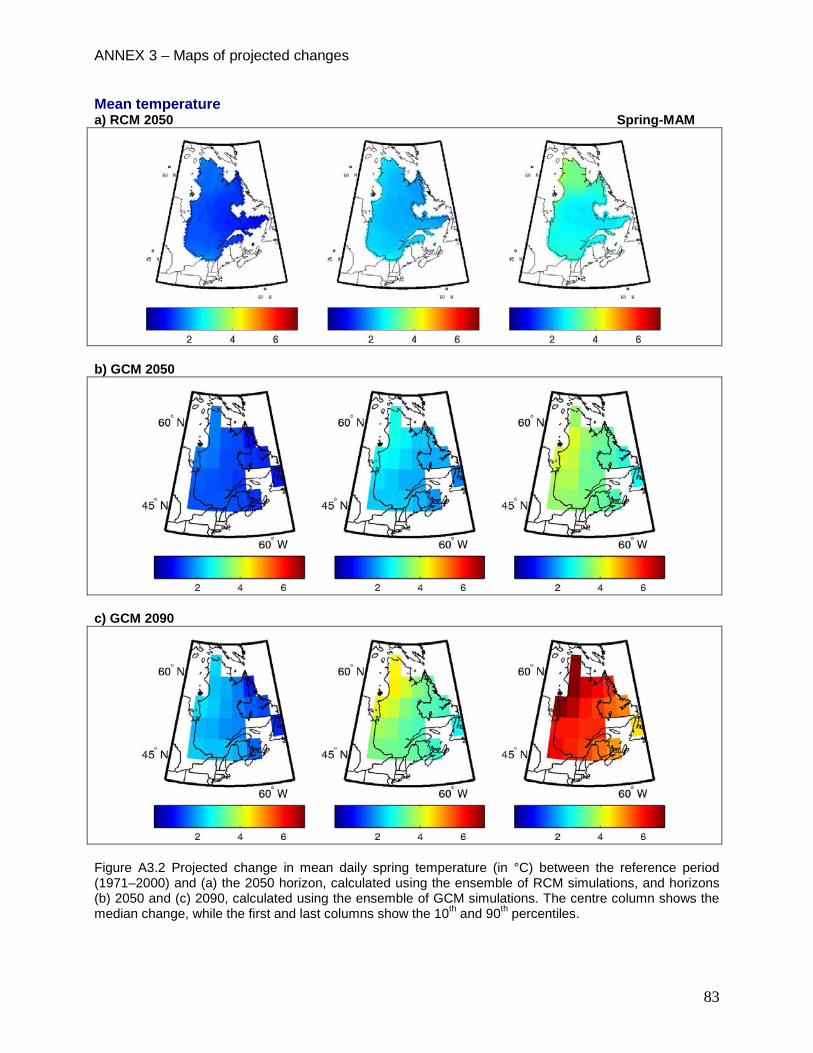
ANNEX 3 – Maps of projected changes
83
Mean temperature a) RCM 2050 Spring-MAM
b) GCM 2050
c) GCM 2090
Figure A3.2 Projected change in mean daily spring temperature (in °C) between the reference period (1971–2000) and (a) the 2050 horizon, calculated using the ensemble of RCM simulations, and horizons (b) 2050 and (c) 2090, calculated using the ensemble of GCM simulations. The centre column shows the median change, while the first and last columns show the 10th and 90th percentiles.

ANNEX 3 – Maps of projected changes
84
Mean temperature a) RCM 2050 Summer-JJA
b) GCM 2050
c) GCM 2090
Figure A3.3 Projected change in mean daily summer temperature (in °C) between the reference period (1971–2000) and (a) the 2050 horizon, calculated using the ensemble of RCM simulations, and horizons (b) 2050 and (c) 2090, calculated using the ensemble of GCM simulations. The centre column shows the median change, while the first and last columns show the 10th and 90th percentiles.

ANNEX 3 – Maps of projected changes
85
Mean temperature a) RCM 2050 Fall SON
b) GCM 2050
c) GCM 2090
Figure A3.4 Projected change in mean daily fall temperature (in °C) between the reference period (1971–2000) and (a) the 2050 horizon, calculated using the ensemble of RCM simulations, and horizons (b) 2050 and (c) 2090, calculated using the ensemble of GCM simulations. The centre column shows the median change, while the first and last columns show the 10th and 90th percentiles.

ANNEX 3 - Maps of projected changes
86
Minimum temperature a) RCM 2050 Winter-DJF
b) GCM 2050
c) GCM 2090
Figure A3.5 Projected change in minimum daily winter temperature (in °C) between the reference period (1971–2000) and (a) the 2050 horizon, calculated using the ensemble of RCM simulations, and horizons (b) 2050 and (c) 2090, calculated using the ensemble of GCM simulations. The centre column shows the median change, while the first and last columns show the 10th and 90th percentiles.

ANNEX 3 - Maps of projected changes
87
Minimum temperature a) RCM 2050 Spring-MAM
b) GCM 2050
c) GCM 2090
Figure A3.6 Projected change in minimum daily spring temperature (in °C) between the reference period (1971–2000) and (a) the 2050 horizon, calculated using the ensemble of RCM simulations, and horizons (b) 2050 and (c) 2090, calculated using the ensemble of GCM simulations. The centre column shows the median change, while the first and last columns show the 10th and 90th percentiles.

ANNEX 3 - Maps of projected changes
88
Minimum temperature a) RCM 2050 Summer JJA
b) GCM 2050
c) GCM 2090
Figure A3.7 Projected change in minimum daily summer temperature (in °C) between the reference period (1971–2000) and (a) the 2050 horizon, calculated using the ensemble of RCM simulations, and horizons (b) 2050 and (c) 2090, calculated using the ensemble of GCM simulations. The centre column shows the median change, while the first and last columns show the 10th and 90th percentiles.
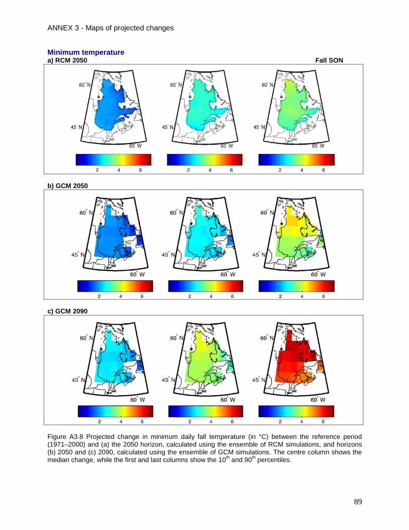
ANNEX 3 - Maps of projected changes
89
Minimum temperature a) RCM 2050 Fall SON
b) GCM 2050
c) GCM 2090
Figure A3.8 Projected change in minimum daily fall temperature (in °C) between the reference period (1971–2000) and (a) the 2050 horizon, calculated using the ensemble of RCM simulations, and horizons (b) 2050 and (c) 2090, calculated using the ensemble of GCM simulations. The centre column shows the median change, while the first and last columns show the 10th and 90th percentiles.

ANNEX 3 - Maps of projected changes
90
Maximum temperature a) RCM 2050 Winter-DJF
b) GCM 2050
c) GCM 2090
Figure A3.9. Projected change in maximum daily winter temperature (in °C) between the reference period (1971–2000) and (a) the 2050 horizon, calculated using the ensemble of RCM simulations, and horizons (b) 2050 and (c) 2090, calculated using the ensemble of GCM simulations. The centre column shows the median change, while the first and last columns show the 10th and 90th percentiles.

ANNEX 3 - Maps of projected changes
91
Maximum temperature a) RCM 2050 Spring-MAM
b) GCM 2050
c) GCM 2090
Figure A3.10 Projected change in maximum daily spring temperature (in °C) between the reference period (1971–2000) and (a) the 2050 horizon, calculated using the ensemble of RCM simulations, and horizons (b) 2050 and (c) 2090, calculated using the ensemble of GCM simulations. The centre column shows the median change, while the first and last columns show the 10th and 90th percentiles.
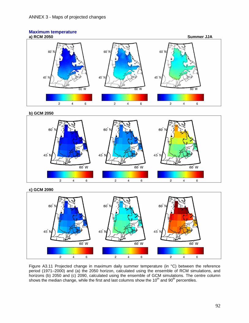
ANNEX 3 - Maps of projected changes
92
Maximum temperature a) RCM 2050 Summer JJA
b) GCM 2050
c) GCM 2090
Figure A3.11 Projected change in maximum daily summer temperature (in °C) between the reference period (1971–2000) and (a) the 2050 horizon, calculated using the ensemble of RCM simulations, and horizons (b) 2050 and (c) 2090, calculated using the ensemble of GCM simulations. The centre column shows the median change, while the first and last columns show the 10th and 90th percentiles.
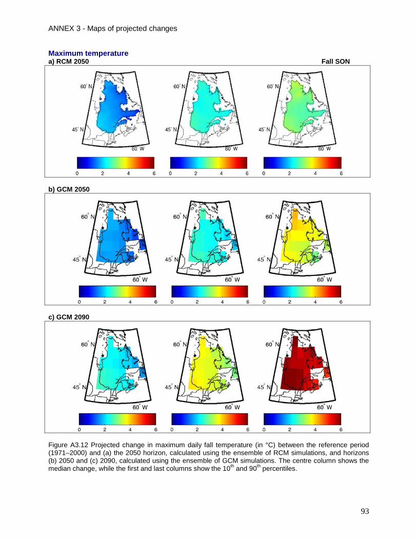
ANNEX 3 - Maps of projected changes
93
Maximum temperature a) RCM 2050 Fall SON
b) GCM 2050
c) GCM 2090
Figure A3.12 Projected change in maximum daily fall temperature (in °C) between the reference period (1971–2000) and (a) the 2050 horizon, calculated using the ensemble of RCM simulations, and horizons (b) 2050 and (c) 2090, calculated using the ensemble of GCM simulations. The centre column shows the median change, while the first and last columns show the 10th and 90th percentiles.
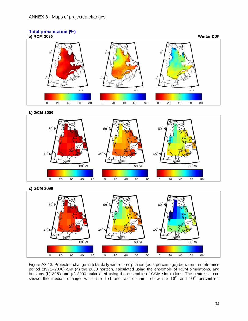
ANNEX 3 - Maps of projected changes
94
Total precipitation (%) a) RCM 2050 Winter DJF
b) GCM 2050
c) GCM 2090
Figure A3.13. Projected change in total daily winter precipitation (as a percentage) between the reference period (1971–2000) and (a) the 2050 horizon, calculated using the ensemble of RCM simulations, and horizons (b) 2050 and (c) 2090, calculated using the ensemble of GCM simulations. The centre column shows the median change, while the first and last columns show the 10th and 90th percentiles.

ANNEX 3 - Maps of projected changes
95
Total precipitation (mm) a) RCM 2050 Winter-DJF
b) GCM 2050
c) GCM 2090
Figure A3.14 Projected change in total daily winter precipitation (in mm) between the reference period (1971–2000) and (a) the 2050 horizon, calculated using the ensemble of RCM simulations, and horizons (b) 2050 and (c) 2090, calculated using the ensemble of GCM simulations. The centre column shows the median change, while the first and last columns show the 10th and 90th percentiles.

ANNEX 3 - Maps of projected changes
96
Total precipitation (%) a) RCM 2050 Spring-MA
b) GCM 2050
c) GCM 2090
Figure A3.15 Projected change in total daily spring precipitation (as a percentage) between the reference period (1971–2000) and (a) the 2050 horizon, calculated using the ensemble of RCM simulations, and horizons (b) 2050 and (c) 2090, calculated using the ensemble of GCM simulations. The centre column shows the median change, while the first and last columns show the 10th and 90th percentiles.

ANNEX 3 - Maps of projected changes
97
Total precipitation (mm) a) RCM 2050 Spring-MAM
b) GCM 2050
c) GCM 2090
Figure A3.16 Projected change in total daily spring precipitation (in mm) between the reference period (1971–2000) and (a) the 2050 horizon, calculated using the ensemble of RCM simulations, and horizons (b) 2050 and (c) 2090, calculated using the ensemble of GCM simulations. The centre column shows the median change, while the first and last columns show the 10th and 90th percentiles.
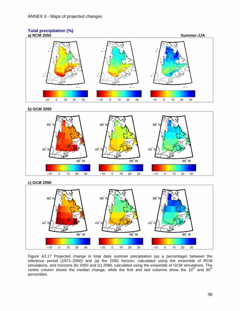
ANNEX 3 - Maps of projected changes
98
Total precipitation (%) a) RCM 2050 Summer-JJA
b) GCM 2050
c) GCM 2090
Figure A3.17 Projected change in total daily summer precipitation (as a percentage) between the reference period (1971–2000) and (a) the 2050 horizon, calculated using the ensemble of RCM simulations, and horizons (b) 2050 and (c) 2090, calculated using the ensemble of GCM simulations. The centre column shows the median change, while the first and last columns show the 10th and 90th percentiles.

ANNEX 3 - Maps of projected changes
99
Total precipitation (mm) a) RCM 2050 Summer-JJA
b) GCM 2050
c) GCM 2090
Figure A3.18 Projected change in total daily summer precipitation (in mm) between the reference period (1971–2000) and (a) the 2050 horizon, calculated using the ensemble of RCM simulations, and horizons (b) 2050 and (c) 2090, calculated using the ensemble of GCM simulations. The centre column shows the median change, while the first and last columns show the 10th and 90th percentiles.

ANNEX 3 - Maps of projected changes
100
Total precipitation (%) a) RCM 2050 Fall-SON
b) GCM 2050
c) GCM 2090
Figure A3.19 Projected change in total daily fall precipitation (as a percentage) between the reference period (1971–2000) and (a) the 2050 horizon, calculated using the ensemble of RCM simulations, and horizons (b) 2050 and (c) 2090, calculated using the ensemble of GCM simulations. The centre column shows the median change, while the first and last columns show the 10th and 90th percentiles

ANNEX 3 - Maps of projected changes
101
Total precipitation (mm) a) RCM 2050 Fall-SON
b) GCM 2050
c) GCM 2090
Figure A3.20 Projected change in total daily fall precipitation (in mm) between the reference period (1971–2000) and (a) the 2050 horizon, calculated using the ensemble of RCM simulations, and horizons (b) 2050 and (c) 2090, calculated using the ensemble of GCM simulations. The centre column shows the median change, while the first and last columns show the 10th and 90th percentiles.

ANNEX 3 - Maps of projected changes
102
Snowfall precipitation (%) a) RCM 2050 Winter-DJF
b) GCM 2050
c) GCM 2090
Figure A3.21 Projected change in daily winter snowfall precipitation (as a percentage) between the reference period (1971–2000) and (a) the 2050 horizon, calculated using the ensemble of RCM simulations, and horizons (b) 2050 and (c) 2090, calculated using the ensemble of GCM simulations. The centre column shows the median change, while the first and last columns show the 10th and 90th percentiles.

ANNEX 3 - Maps of projected changes
103
Snowfall precipitation (mm) a) RCM 2050 Winter-DJF
b) GCM 2050
c) GCM 2090
Figure A3.22 Projected change in daily winter snowfall precipitation (in mm) between the reference period (1971–2000) and (a) the 2050 horizon, calculated using the ensemble of RCM simulations, and horizons (b) 2050 and (c) 2090, calculated using the ensemble of GCM simulations. The centre column shows the median change, while the first and last columns show the 10th and 90th percentiles.

ANNEX 3 - Maps of projected changes
104
Snowfall precipitation (%) a) RCM 2050 Spring-MAM
b) GCM 2050
c) GCM 2090
Figure A3.23 Projected change in daily spring snowfall precipitation (as a percentage) between the reference period (1971–2000) and (a) the 2050 horizon, calculated using the ensemble of RCM simulations, and horizons (b) 2050 and (c) 2090, calculated using the ensemble of GCM simulations. The centre column shows the median change, while the first and last columns show the 10th and 90th percentiles.
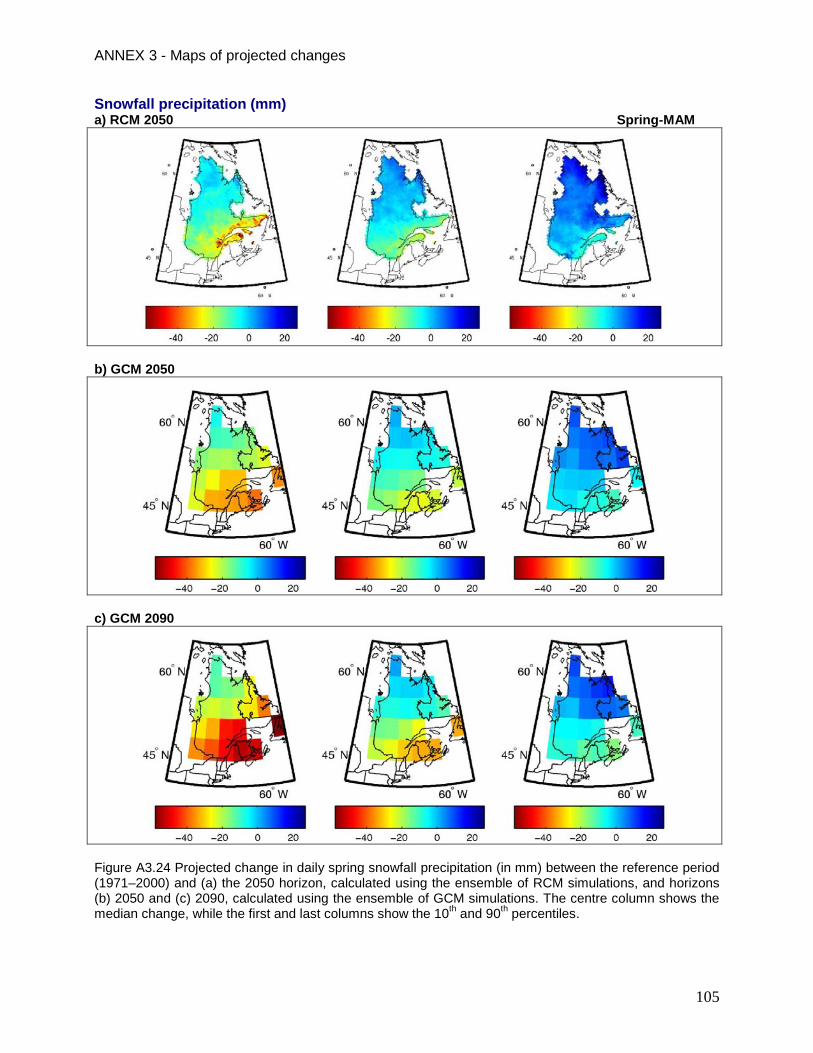
ANNEX 3 - Maps of projected changes
105
Snowfall precipitation (mm) a) RCM 2050 Spring-MAM
b) GCM 2050
c) GCM 2090
Figure A3.24 Projected change in daily spring snowfall precipitation (in mm) between the reference period (1971–2000) and (a) the 2050 horizon, calculated using the ensemble of RCM simulations, and horizons (b) 2050 and (c) 2090, calculated using the ensemble of GCM simulations. The centre column shows the median change, while the first and last columns show the 10th and 90th percentiles.

ANNEX 3 - Maps of projected changes
106
Snowfall precipitation (%) a) RCM 2050 Fall-SON
b) GCM 2050
c) GCM 2090
Figure A3.25 Projected change in daily fall snowfall precipitation (as a percentage) between the reference period (1971–2000) and (a) the 2050 horizon, calculated using the ensemble of RCM simulations, and horizons (b) 2050 and (c) 2090, calculated using the ensemble of GCM simulations. The centre column shows the median change, while the first and last columns show the 10th and 90th percentiles.
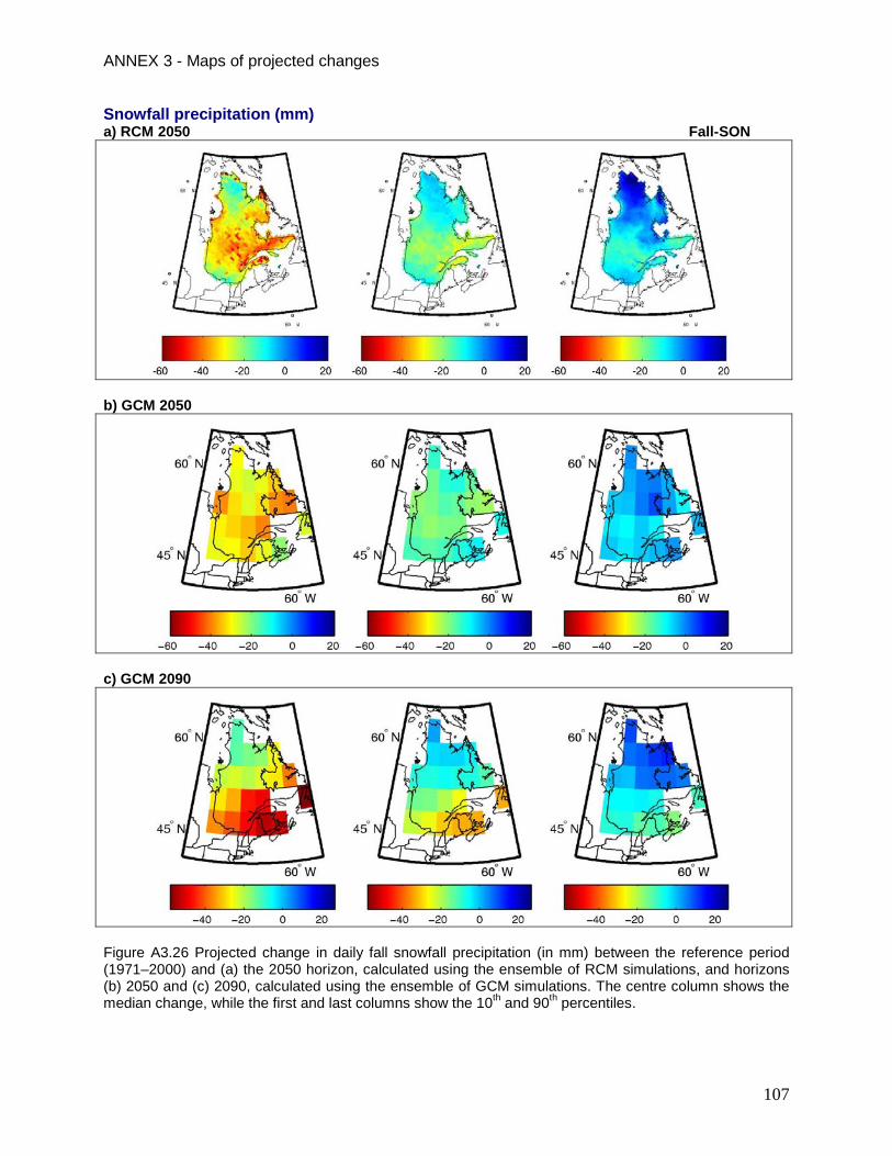
ANNEX 3 - Maps of projected changes
107
Snowfall precipitation (mm) a) RCM 2050 Fall-SON
b) GCM 2050
c) GCM 2090
Figure A3.26 Projected change in daily fall snowfall precipitation (in mm) between the reference period (1971–2000) and (a) the 2050 horizon, calculated using the ensemble of RCM simulations, and horizons (b) 2050 and (c) 2090, calculated using the ensemble of GCM simulations. The centre column shows the median change, while the first and last columns show the 10th and 90th percentiles.

ANNEX 3 - Maps of projected changes
108
Freeze/Thaw Events a) RCM 2050 Winter-DJF
b) MCG 2050
c) GCM 2090
Figure A3.27 Projected change in the number of winter freeze/thaw events (in days) between the reference period (1971–2000) and (a) the 2050 horizon, calculated using the ensemble of RCM simulations, and horizons (b) 2050 and (c) 2090, calculated using the ensemble of GCM simulations. The centre column shows the median change, while the first and last columns show the 10th and 90th percentiles.
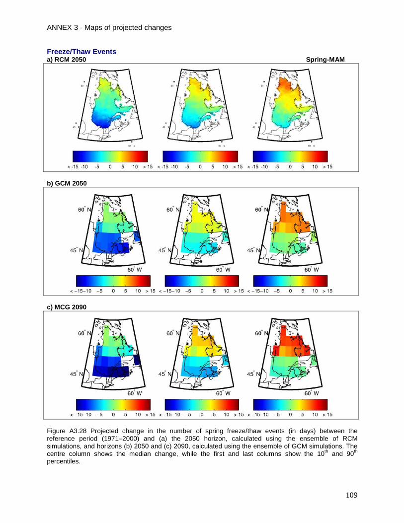
ANNEX 3 - Maps of projected changes
109
Freeze/Thaw Events a) RCM 2050 Spring-MAM
b) GCM 2050
c) MCG 2090
Figure A3.28 Projected change in the number of spring freeze/thaw events (in days) between the reference period (1971–2000) and (a) the 2050 horizon, calculated using the ensemble of RCM simulations, and horizons (b) 2050 and (c) 2090, calculated using the ensemble of GCM simulations. The centre column shows the median change, while the first and last columns show the 10th and 90th percentiles.
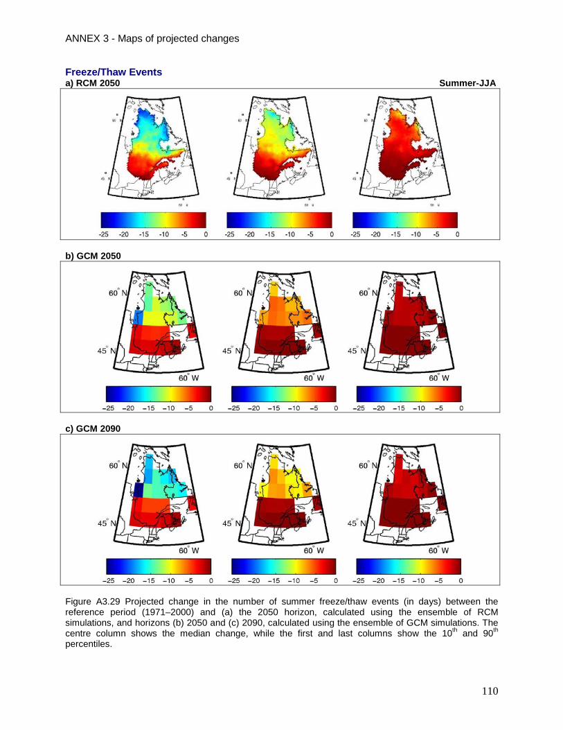
ANNEX 3 - Maps of projected changes
110
Freeze/Thaw Events a) RCM 2050 Summer-JJA
b) GCM 2050
c) GCM 2090
Figure A3.29 Projected change in the number of summer freeze/thaw events (in days) between the reference period (1971–2000) and (a) the 2050 horizon, calculated using the ensemble of RCM simulations, and horizons (b) 2050 and (c) 2090, calculated using the ensemble of GCM simulations. The centre column shows the median change, while the first and last columns show the 10th and 90th percentiles.

ANNEX 3 - Maps of projected changes
111
Freeze/Thaw Events a) RCM 2050 Fall-SON
b) GCM 2050
c) GCM 2090
Figure A3.30 Projected change in the number of fall freeze/thaw events (in days) between the reference period (1971–2000) and (a) the 2050 horizon, calculated using the ensemble of RCM simulations, and horizons (b) 2050 and (c) 2090, calculated using the ensemble of GCM simulations. The centre column shows the median change, while the first and last columns show the 10th and 90th percentiles.

ANNEX 3 - Maps of projected changes
112
Freeze/Thaw Events a) RCM 2050 Annual
b) GCM 2050
c) GCM 2090
Figure A3.31 Projected change in the number of annual freeze/thaw events between the reference period (1971–2000) and (a) the 2050 horizon, calculated using the ensemble of RCM simulations, and horizons (b) 2050 and (c) 2090, calculated using the ensemble of GCM simulations. The centre column shows the median change, while the first and last columns show the 10th and 90th percentiles.

ANNEX 3 - Maps of projected changes
113
Growing-Degree Days a) RCM 2050 Annual
b) GCM 2050
c) GCM 2090
Figure A3.32 Projected change in the number of growing degree-days between the reference period (1971–2000) and (a) the 2050 horizon, calculated using the ensemble of RCM simulations, and horizons (b) 2050 and (c) 2090, calculated using the ensemble of GCM simulations. The centre column shows the median change, while the first and last columns show the 10th and 90th percentiles.
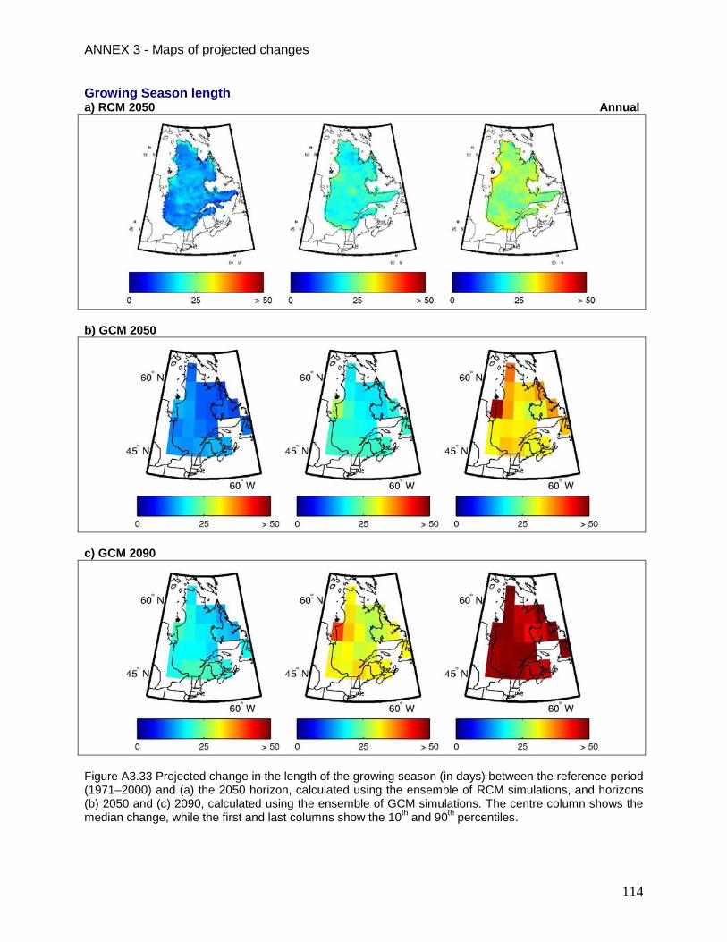
ANNEX 3 - Maps of projected changes
114
Growing Season length a) RCM 2050 Annual
b) GCM 2050
c) GCM 2090
Figure A3.33 Projected change in the length of the growing season (in days) between the reference period (1971–2000) and (a) the 2050 horizon, calculated using the ensemble of RCM simulations, and horizons (b) 2050 and (c) 2090, calculated using the ensemble of GCM simulations. The centre column shows the median change, while the first and last columns show the 10th and 90th percentiles.

ANNEX 3 - Maps of projected changes
115
Canadian Drought Code a) RCM 2050
b) GCM 2050
c) GCM 2090
Figure A3.34 Projected change in the Canadian drought index for April to October between the reference period (1971–2000) and (a) the 2050 horizon, calculated using the ensemble of RCM simulations, and horizons (b) 2050 and (c) 2090, calculated using the ensemble of GCM simulations. The centre column shows the median change, while the first and last columns show the 10th and 90th percentiles.

ANNEX 4 – Detailed methodology
116
Annex 4 Detailed methodology A4.1 Cluster analysis An ensemble of climate simulations is, to date, the best estimator of simulated future climate as it covers principle sources of uncertainty (Gleckler et al. 2008). Currently, no methodological technique allows a reduction in the total ensemble uncertainty, and consequently, adequate coverage of this uncertainty is a priority when climate scenarios are provided to climate change adaptation decision-makers. As such, in an ideal situation, projects that require climate scenarios would incorporate a large ensemble of climate simulations in order to obtain the best possible estimation of the future climate and its associated uncertainty. However, there can also be imbalances in the ensemble when a large proportion of the simulation comes from a single climate model. This problem occurred with the Atlas given that out of the available regional
simulations, 12 out 18 were produced from the combination of one regional model and one GCM pilot, namely the CRCM4 and CGCM3 (Table A4.1). One must note that the problem is not as important for the global simulations where the selected ensemble came from a large number of GCM models present in the 2007 IPCC report (Meehl et al. 2007). In order to diminish the imbalance, a smaller number of simulations must be selected. The selection method utilised here is cluster analysis, a statistical data classification technique. Cluster analysis is advantageous as it allows a reduction in the number of simulations used while conserving an adequate coverage of the variability present in the ensemble. This method also offers ways to objectively determine the number of groups based on a large number of dimensions and variables directly linked to the processes of interest in the study.
Table A4.1 Summary of available regional climate simulations
RCM Domain Pilot Pilot Member SRES Source CRCM4.1.1 QC CGCM3 4 A2 Ouranos
CRCM4.1.1 QC CGCM3 5 A2 Ouranos
CRCM4.2.0 AMNO CGCM2 3 A2 Ouranos
CRCM4.2.0 AMNO CGCM3 4 A2 Ouranos
CRCM4.2.0 AMNO CGCM3 5 A2 Ouranos
CRCM4.2.3 AMNO CGCM3 1 A2 Ouranos
CRCM4.2.3 AMNO CGCM3 2 A2 Ouranos
CRCM4.2.3 AMNO CGCM3 3 A2 Ouranos
CRCM4.2.3 AMNO CGCM3 4 A2 Ouranos
CRCM4.2.3 AMNO CGCM3 5 A2 Ouranos
CRCM4.2.3 QC CGCM3 4 A2 Ouranos
CRCM4.2.3 QC CGCM3 5 A2 Ouranos
CRCM4.2.3 AMNO ECHAM5 1 A2 Ouranos
CRCM4.2.3 QC ECHAM5 1 A2 Ouranos
ARPEGE-CLIMAT/Ouranos
WINN* N/A 1 A2 Ouranos
ARPEGE-CLIMAT/Ouranos
WINN* N/A 2 A2 Ouranos
HRM3 NARCCAP HADCM3 A2 NARCCAP
RCM3 NARCCAP CGCM3 A2 NARCCAP Note: The scenarios in blue represent those selected using cluster analysis. *The ARPEGE-CLIMAT/Ouranos model produces simulations on a variable global domain. The « WINN » grid is stretched to produce a concentration of points over North America (centered on Winnipeg 50°N 95°O) and produced a spatial resolution of ~50KM at the center of the grid.
ANNEX 4 – Detailed methodology
117
Description of the cluster analysis Cluster analyses belong to a family of statistical methods utilised to classify data into a smaller number of sub-groups. These sub-groups are based on an analysis of similarities between the data. More specifically, the Atlas used k-means clustering which groups the data by maximizing the variability between groups and minimizing the variability within groups. In this case the K-means clustering was performed as an unsupervised classification, where no a priori information on the structure of the groups is provided or required. Method The first step in a cluster analysis consists of determining the climate variables of interest for the project. In the case of the Atlas, these variables are mean temperature, total precipitation, snow precipitation, freeze/thaw cycles, growing degree-days, growing season length, and the Canadian drought code. Secondly, for the available ensemble of eighteen regional climate simulations, the seasonal Δs of each variable are calculated for the future horizon of interest (2050) over the study area. Deltas values are then normalized in order to avoid differences in units between variables from influencing the grouping. A series of k-means cluster analyses is then conducted, varying the numbers of groups from 2 to 18. Each grouping is done using the normalized seasonal Δs. The distance between the groups for each grouping (2 to 18 groups) is evaluated with a R2 statistics. These R2 values are graphically represented with a profile (Figure A4.1) that is used to determine the number of groups that should be kept. For the selected groups, the climate simulation that is closest to the center of each group is retained for the analyses and the production of maps in the Atlas (Figure A4.2). Results of the cluster analysis The R2 profile (Figure A4.1) shows that R2 increases with an increase in the number of groups. However, we observe a levelling off of
the profile starting at approximately eight groups (in this case) where an increase in the number of groups has little impact of the coverage of the total variance. This levelling off, along with the fact that the threshold of 8 groups corresponds to 90% of the total variance, are the reasons why eight groups were selected for the Atlas. The 8 simulations closest to the centroid of each group were then selected for all further analyses (Table A4.2). The results of this selection are presented in Figure A4.2, which allows a visualization of the coverage of the total variance offered by the 8 selected simulations for the projected changes of each variable of interest. We observe that for each dimension along the x-axis, the coverage of the variability with the selected scenarios is adequate (Figure A4.2). More precisely, we observe that the 8 selected scenarios, represented by colored circles on the figure, adequately cover the range in values associated with the 18 original scenarios, represented by grey circles. Note that, in certain cases, the cluster analysis reduced the redundancy in the original RCM ensemble, for example with the growing degree-days where there was originally, a high number of very similar scenarios (Figure A4.2). To validate the selection we point out that the results of the cluster analysis correspond to research conclusions on the sources of uncertainties of climate projections. In Table A4.1, we see that the selected simulations mainly come from a mix of different GCM pilots and different RCM models, and that the discarded simulations were mainly simulations stemming from the combination of a RCM pilot where there were a number of members in the ensemble. Given that the objective of the cluster analysis is to maximize uncertainty coverage and to reduce the redundancy in the RCM ensemble, our selection corresponds to the conclusions of Déqué et al. (2007), who observed that, in general, the largest source of variance stems from the choice of the GCM pilot but that for precipitation projections, the choice of the RCM has an more or less influence to that of the pilot. Déqué et al. (2007) also show that the role of the members and of the SRES scenario is reduced compared to the GCM and RCM. Another study (de Elía et al. 2008) comes to similar conclusions as to the role of the pilot and the RCM on the uncertainty of the projections and also demonstrates the smaller role of the RCM domain as a source of uncertainty compared to the pilot and RCM.

ANNEX 4 – Detailed methodology
118
Figure A4.1 R2 profile of cluster analyses. The blue curve presents the R2 values from the series of cluster analyses conducted on the seasonal Δs as a function of the number of groups.

ANNEX 4 – Detailed methodology
119
Figure A4.2 Visualisation of the coverage of the total variance obtained using the selected scenarios. Grey circles represent standardized monthly Δs for the regional ensemble of 18 simulations. Coloured circles represent the 8 selected scenarios for the Atlas.

ANNEX 4 – Detailed methodology
120
A4.2 Evaluation of the climate models for the period 1971-2000
Gleckler et al. (2008) demonstrated that the ensemble median or mean is the most dependable way to estimate observed climate conditions over large portions of the globe. As such, in the production of the Atlas it was deemed neccessary to conduct a similar evaluation of the climate simulations (using the method described by Gleckler et al. 2008) to validate whether these conclusions are applicable in a more regional context such as that of the territory of Québec. Reference data In order to conduct an evaluation, the outputs from the climate models must be compared with reference data. For this evaluation, data provided by the NLWIS (National Land and Water Information Service) were chosen. The data are provided on a regular grid with a spatial resolution of 10 km × 10 km covering Canada south of 60°N. All climate models available through the Program for Climate Model Diagnosis and Intercomparison (PCMDI, Meehl et al. 2007) were included in the analysis. Regional models selected with the cluster analysis were also included. A summary
of the climate models included in the evaluation is presented in Table A4.2. Study area and reference grid
Reference data and climate models all have different grids and resolutions. It is therefore necessary to establish a common study area and reference grid in order to consistently evaluate the variables produced by the models (Figure A4.3). The chosen validation grid is the section of the Canadian global model grid (CGCM3 T47) that intersects the reference data from the NLWIS and the data from the regional models. More specifically, only the grid cells that are covered by the NLWIS data by more than ~40% are kept in the analysis. In addition, only grid cells with more than 50% of land according to the land-sea mask were included. The climate data of each model and of the NLWIS are then interpolated to this validation grid for comparison. For the GCM data, this meant taking the value at the model grid point nearest the reference grid cell centroid, while for NLWIS and MRC data, it meant calculating the arithmetic mean for all points falling inside each of the reference grid cells.

ANNEX 4 – Detailed methodology
121
Figure A4.3 Common validation grid over Québec, to the right in red, which intersects the reference grids for the GCMs and RCMs as well as the grid of NLWIS observed normals.
Table A4.2 Summary of climate models included in the evaluation
Centre/Modeling program Country Models
Ouranos Canada
ARPEGE-CLIMAT/Ouranos CRCM4.2.0_CGCM2 CRCM4.2.3_CGCM3 CRCM4.2.3_ECHAM5
North American Regional Climate Change Assessment Program United States HRM3_HADCM3 RCM3_CGCM3
Canadian Centre for Climate Modelling & Analysis Canada CCCMA_CGCM3_1
CSIRO Atmospheric Research Australia CSIRO_Mk3_0
CSIRO Atmospheric Research Australia CSIRO_Mk3_5
U.S. Dept. of Commerce/NOAA/Geophysical fluid dynamics laboratory United States GFDL_CM_2_0
NASA/Goddard Institute for Space Studies United States GISS_AOM
Instituto Nazionale di Geofisica e Vulcanologia Italy INGV_ECHAM4
Institut Pierre Simon Laplace France IPSL_CM4
Center for Climate System Research (The University of Tokyo), National Institute for Environmental Studies, and Frontier Research Center for Global Change (JAMSTEC)
Japan MIROC3_2_medres
Meteorological Institute of the University of Bonn, Meteorological Research Institute of KMA, and Model and Data group. Korea MIUB_ECHO_G
Max Planck Institute for Meteorology Germany MPI_ECHAM5
Meteorological Research Institute Japan MRI_CGCM2_3_2a
ANNEX 4 – Detailed methodology
122
Calculation of the spatial and temporal in relation to the average climate As mentioned above, the methodology proposed by Gleckler et al. (2008) was used to evaluate the models. For each model, m, and variable f, a global normalized error E’mf, is calculated on the validation grid using:
f
fmfmf E
EEE
−='
(1)
wherefE is the ensemble mean of errors for
the variable f, which is calculated according to:
fE =1M Emfm=1
M
∑ (2)
where M is the total number of global and regional simulations in the ensemble1 and Emf is the mean quadratic error between a model m and the reference r (NLWIS) for a variable f over the validation grid, calculated according to:
( )∑∑
==
−=T
tritmit
I
iTImf ffE
1
2
1
11
(3)
Emf is the quadratic sum between the climate normal within a simulated field mit and the climate normal for a reference field rit. The index i represents the spatial dimension (the i tile) and t represents the temporal dimension (either 1 to 12 for monthly variables or 1 for annual variables.
Consequently, when the E’mf value is negative, the model m performs better than the mean of the ensemble, while a positive value indicates a below-mean performance. Figure A4.4 presents a summary of the relative errors (E’mf) calculated for different climate indices. Calculation of mean annual cycles The mean annual cycle is estimated either with observed data or with model outputs. It is estimated by calculating the climatic normal of each month over a given region. In our case, the monthly normals of each variable (f) are calculated for the reference period over the entire validation area. They are calculated for each regional and global simulation and for the
observed data from the NLWIS, according to:
mtf =1I mitf
i=1
I
∑ (4)
or
rtf =1I ritf
i=1
I
∑ (5)
Mean annual cycles are presented in Figures A4.5 to A.4.11. The median RCM1 and median GCM2 models are also represented. The annual cycles are not presented for growing season length and the Canadian drought code variables, which are calculated on an annual basis. These variables are therefore presented using dispersion diagrams (A4.12).
A4.3 Results of the climate model evaluation Figure A4.4 presents a summary of the relative errors (E’mf) calculated for the different climatic variables. The first column presents the results for the median RCM3 and GCM4 models while the other columns show the results for the individual models. The results of this evaluation of the climate models demonstrates that, over Quebec, the median of a large ensemble of climate simulations produces more constant results over the ensemble of variables. The evaluation suggests that no one individual model can be selected as the best performer for all variables of interest. In addition, we note that the different members1 of a model perform in a similar fashion. Figures A4.5 to 4.12 present the results (1971-2000) for each variable of interest over Quebec. These results show that while the median of the ensemble is not always the best at reproducing the annual cycles of individual variables, it is nonetheless often very close to the observed cycle. This therefore complements the results of Gleckler et al (2008) over large global regions. 1 M = 29 is superior to the number of models presented in Table A2 because some models have numerous members 2 median RCM modele: a fictitious simulation of a RCM that would have an identical response to the median of the regional ensemble 3 median GCM model: a fictitious simulation of a GCM that would have an identical response to the median of the global ensemble 4 the members of a model are produced with the same climate model and SRES scenario but with a slight perturbation in the initial conditions
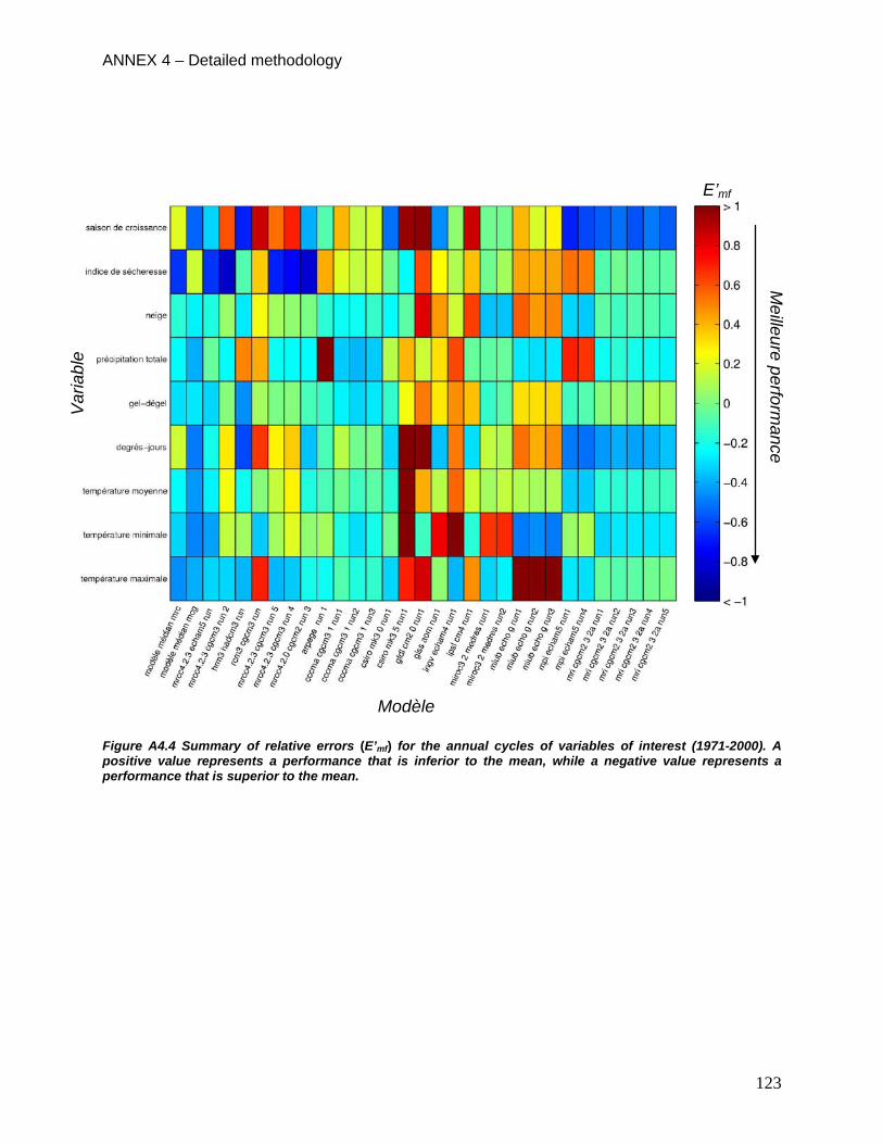
ANNEX 4 – Detailed methodology
123
Figure A4.4 Summary of relative errors (E’mf) for the annual cycles of variables of interest (1971-2000). A positive value represents a performance that is inferior to the mean, while a negative value represents a performance that is superior to the mean.
Var
iabl
e
Meilleure perform
ance
Modèle
E’mf

ANNEX 4 – Detailed methodology
124
Figure A4.5 Comparison of the mean annual cycle of maximum temperature over the reference period (1971-2000): median of the GCM ensemble (blue line), individual GCM simulations (dashed blue lines), MRC simulations (dashed black lines), median of the RCM ensemble (black line), and reference date (red line).
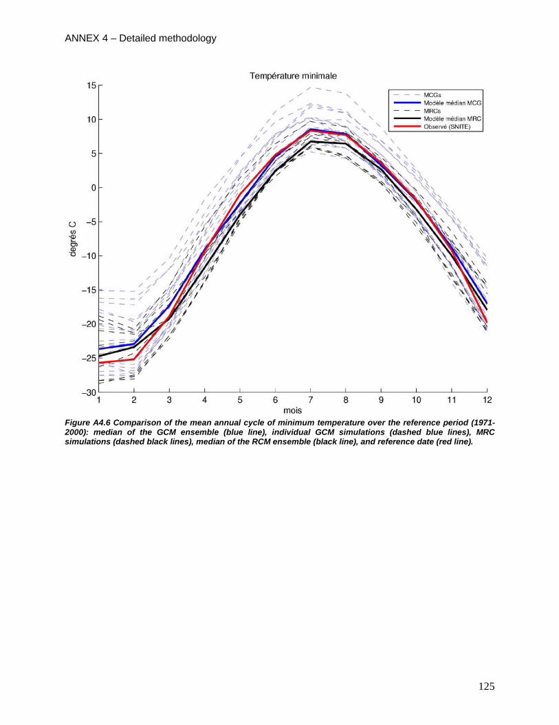
ANNEX 4 – Detailed methodology
125
Figure A4.6 Comparison of the mean annual cycle of minimum temperature over the reference period (1971-2000): median of the GCM ensemble (blue line), individual GCM simulations (dashed blue lines), MRC simulations (dashed black lines), median of the RCM ensemble (black line), and reference date (red line).

ANNEX 4 – Detailed methodology
126
Figure A4.7 Comparison of the mean annual cycle of mean temperature over the reference period (1971-2000): median of the GCM ensemble (blue line), individual GCM simulations (dashed blue lines), MRC simulations (dashed black lines), median of the RCM ensemble (black line), and reference date (red line).

ANNEX 4 – Detailed methodology
127
Figure A4.8 Comparison of the mean annual cycle of total precipitation over the reference period (1971-2000): median of the GCM ensemble (blue line), individual GCM simulations (dashed blue lines), MRC simulations (dashed black lines), median of the RCM ensemble (black line), and reference date (red line).

ANNEX 4 – Detailed methodology
128
Figure A4.9 Comparison du mean annual cycle of snow precipitation over the reference period (1971-2000): median of the GCM ensemble (blue line), individual GCM simulations (dashed blue lines), MRC simulations (dashed black lines), median of the RCM ensemble (black line), and reference date (red line).
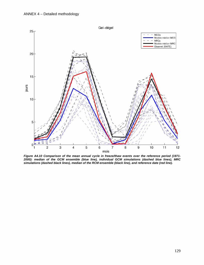
ANNEX 4 – Detailed methodology
129
Figure A4.10 Comparison of the mean annual cycle in freeze/thaw events over the reference period (1971-2000): median of the GCM ensemble (blue line), individual GCM simulations (dashed blue lines), MRC simulations (dashed black lines), median of the RCM ensemble (black line), and reference date (red line).

ANNEX 4 – Detailed methodology
130
Figure A4.11 Comparison of the mean annual cycle in the number of growing degree-days (> 5°C) over the reference period (1971-2000): median of the GCM ensemble (blue line), individual GCM simulations (dashed blue lines), MRC simulations (dashed black lines), median of the RCM ensemble (black line), and reference date (red line).

ANNEX 4 – Detailed methodology
131
Figure A4.12 Comparison of the climate normal of the Canadian drought code and the growing degree days over the reference period (1971-2000): median for the GCM ensemble (blue circles), individual GCM simulations (grey circles), RCM simulations (open black squares), medians for the RCM ensemble (black squares) and reference data (red circles). The results are represented by circles (as opposed to lines) because the data for these two variables is only available on an annual basis (and not monthly).
132
References de Elía R, Caya D, Côté H, Frigon A, Biner S, Giguère M, Paquin D, Harvey R, Plummer D. 2008. Evaluation of uncertainties in the CRCM-simulated North American climate. Clim Dyn. 30:113-132. Déqué M, Rowell DP, Luthi D, Giorgi F, Christensen JH, Rockel B, Jacob D, Kjellstrom E, de Castro M, van den Hurk B. 2007. An intercomparison of regional climate simulations for Europe: assessing uncertainties in model projections. Clim. Change 81:53-70 GIEC. 2007. Bilan 2007 des changements climatiques. Contribution des Groupes de travail I, II et III au quatrième Rapport d’évaluation du Groupe d’experts intergouvernemental sur l’évolution du climat [Équipe de rédaction principale, Pachauri, R.K. et Reisinger, A. (publié sous la direction de~)]. GIEC, Genève, Suisse, …, 103 pages.