Atmospheres and spectra of strongly magnetized neutron stars

Wynn C. G. HoP and Dong LaiP

Center for Radiophysics and Space Research, Department of Astronomy, Cornell University Ithaca, NY 14853, USA

Accepted 2001 July 2. Received 2001 June 27; in original form 2001 April 18

A B S T R A C T

We construct atmosphere models for strongly magnetized neutron stars with surface fields

B , 1012–1015 G and effective temperatures Teff , 106–107 K. The atmospheres directly

determine the characteristics of thermal emission from isolated neutron stars, including radio

pulsars, soft gamma-ray repeaters, and anomalous X-ray pulsars. In our models, the

atmosphere is composed of pure hydrogen or helium and is assumed to be fully ionized. The

radiative opacities include free–free absorption and scattering by both electrons and ions

computed for the two photon polarization modes in the magnetized electron–ion plasma.

Since the radiation emerges from deep layers in the atmosphere with r * 102 g cm23, plasma

effects can significantly modify the photon opacities by changing the properties of the

polarization modes. In the case where the magnetic field and the surface normal are parallel,

we solve the full, angle-dependent, coupled radiative transfer equations for both polarization

modes. We also construct atmosphere models for general field orientations based on the

diffusion approximation of the transport equations and compare the results with models based

on full radiative transport. In general, the emergent thermal radiation exhibits significant

deviation from blackbody, with harder spectra at high energies. The spectra also show a broad

feature ðDE/EBi , 1Þ around the ion cyclotron resonance EBi ¼ 0:63ðZ/AÞðB/1014 GÞ keV,

where Z and A are the atomic charge and atomic mass of the ion, respectively; this feature is

particularly pronounced when EBi * 3kTeff . Detection of the resonance feature would

provide a direct measurement of the surface magnetic fields on magnetars.

Key words: magnetic fields – radiative transfer – stars: atmospheres – stars: magnetic fields –

stars: neutron – X-rays: stars.

1 I N T R O D U C T I O N

Neutron stars (NSs) are created in the core collapse and subsequent

supernova explosion of massive stars and begin their lives at high

temperatures, T * 1011 K. As they cool over the next ,105–106 yr,

they act as sources of soft X-rays with surface temperatures

*105 K. The cooling history of the NS depends on poorly

constrained interior physics such as the nuclear equation of state,

superfluidity, and magnetic field (see, e.g., Tsuruta 1998; Yakovlev

et al. 2001, for a review). Thus observations of surface emission

from isolated NSs can provide invaluable information on the

physical properties and evolution of NSs. In recent years, the

spectra of several radio pulsars (e.g. PSR B1055252, B0656114,

and Geminga) have been observed to possess a thermal component

that can be attributed to the surface emission at temperatures in the

range ð2–10Þ � 105 K, while a few other pulsars show thermal

emission from hot spots at temperatures of a few times 106 K on the

NS surface (e.g., for observations in the X-rays, see Becker &

Trumper 1997; Becker 2000; in the extreme ultraviolet, Edelstein,

Foster & Bowyer 1995; Korpela & Bowyer 1998; in the optical

band, Pavlov, Welty & Cordova 1997; Caraveo et al. 2000). In

addition, several radio-quiet, isolated NSs, presumably accreting

from the interstellar medium (see Treves et al. 2000), have been

detected in the X-ray and optical bands (e.g. Caraveo, Bignami &

Trumper 1996; Walter, Wolk & Neuhauser 1996; Walter &

Matthews 1997; Caraveo 1998; Mignani, Caraveo & Bignami

1998; Paerels et al. 2001). Recent observations by the Chandra

X-ray Observatory have also revealed a number of compact central

sources in supernova remnants with spectra consistent with thermal

emission from isolated NSs (see Pavlov 2000). Most interestingly,

in the last few years, thermal radiation has been detected from a

potentially new class of NSs, ‘magnetars’, which possess

superstrong magnetic fields ðB * 1014 GÞ (Duncan & Thompson

1992; Thompson & Duncan 1993, 1995, 1996; see Thompson 2000

for a review).

Observations of soft gamma-ray repeaters (SGRs) and

anomalous X-ray pulsars (AXPs) strongly suggest that these are

NSs endowed with superstrong magnetic fields (e.g. Vasisht &

Gotthelf 1997; Kouveliotou et al. 1998, 1999; see, e.g., Hurley

PE-mail: wynnho@astro.cornell.edu (WCGH); dong@astro.cornell.edu

(DL)

Mon. Not. R. Astron. Soc. 327, 1081–1096 (2001)

q 2001 RAS

2000 for SGR review; Mereghetti 1999 for AXP review).

According to the magnetar model, the X-ray luminosity from

AXPs and the quiescent X-ray emission from SGRs are powered by

the decay of a superstrong ðB , 1014–1015 GÞ magnetic field

(Thompson & Duncan 1996) and/or by the residual thermal energy

(Heyl & Hernquist 1997a). Alternatively, it has been proposed that

the AXP emission may originate from accretion on to a NS with

B , 1012 G, e.g., from a fossil disc left over from the supernova

explosion (see Alpar 2001; Chatterjee, Hernquist & Narayan 2000,

and references therein). However, detailed timing studies of AXPs

and SGRs (e.g. Thompson et al. 2000; Kaspi et al. 2001) and deep

optical observations (e.g. Hulleman, van Kerkwijk & Kulkarni

2000; Kaplan et al. 2001), as well as the many similarities between

AXPs and SGRs, clearly favour the magnetar model for both AXPs

and SGRs. Nevertheless, it should be emphasized that, like radio

pulsars, the magnetic field strengths ðB , 1014–1015 GÞ of

magnetars are indirectly inferred and are based on the

measurement of the spin periods ð6–12 sÞ and period derivatives

and on the assumption that the spin-down is because of the loss of

angular momentum that is carried away by magnetic dipole

radiation or Alfven waves (Thompson & Blaes 1998; Thompson

et al. 2000). Thermal radiation has already been detected in four of

the five AXPs (1E 1048.125937, 1E 184520258, 4U0142161,

RXS J1708240) and in SGR 1900114; fits to the spectra with

blackbody or with crude atmosphere models indicate that the

thermal X-rays can be attributed to magnetar surface emission at

temperatures of ð3–7Þ � 106 K (see Mereghetti 1999; Perna et al.

2001). Clearly, detailed observational and theoretical studies of

thermal emission can potentially reveal much about the physical

conditions and the true nature of magnetars. Of particular

importance are possible spectral features, such as the ion cyclotron

line (see equation 1.1) studied in this paper (see also Zane et al.

2001), which, if detected, can provide a direct measurement of the

surface magnetic field. In fact, it has been suggested that the lack of

proton and electron cyclotron features in XMM – Newton

observations of the isolated NS RX J0720.423125 may lead to

constraints on its surface magnetic field (Paerels et al. 2001).

Thermal radiation from a magnetized NS is mediated by the thin

atmospheric layer (with scaleheight ,0:1–10 cm and density

,0:1–100 g cm23Þ that covers the stellar surface. The physical

properties of the atmosphere, such as the chemical composition,

equation of state, and especially the radiative opacities, directly

determine the characteristics of the thermal emission. While the

surface composition of the NS is unknown, a great simplification

arises because of the efficient gravitational separation of light and

heavy elements (with time-scales of the order of seconds; see

Alcock & Illarionov 1980 for a discussion of gravitational

separation in white dwarfs). A pure H atmosphere is expected even

if a small amount of fallback/accretion occurs after NS formation.1

A pure He atmosphere results if H is completely burnt up, and a

pure Fe atmosphere may be possible if no fallback/accretion

occurs.

Steady progress has been made over the years in modelling NS

atmospheres. The first models of zero-field NS atmospheres were

constructed by Romani (1987). Later works used improved opacity

and equation of state data from the OPAL project for pure

hydrogen, helium, and iron compositions (Rajagopal & Romani

1996; Zavlin, Pavlov & Shibanov 1996). These works showed that

the radiation spectra from light element (H or He), low-field ðB &

108 GÞ atmospheres deviate significantly from blackbody spectra.

Magnetic NS atmosphere modelling was first attempted by Miller

(1992), who unfortunately adopted an incorrect polarization-

averaging procedure for the radiative transport and included only

bound-free opacities. So far the most comprehensive studies of

magnetic NS atmospheres have focused on hydrogen and moderate

field strengths of B , 1012–1013 G (Shibanov et al. 1992; Pavlov

et al. 1994; see Pavlov et al. 1995 for a review and Zane, Turolla &

Treves 2000 for full, angle-dependent atmosphere models with

accretion). These models correctly take into account the transport

of different photon modes (in the diffusion approximation) through

a mostly ionized medium. The opacities adopted in the models

include free–free transitions and electron scattering, while bound-

free opacities are treated in a highly approximate manner and

bound–bound transitions are completely ignored. Because the

strong magnetic field significantly increases the binding energies of

atoms, molecules, and other bound states (see Lai 2001 for a recent

review), these bound states have appreciable abundances in the

atmosphere at low temperatures ðT & 106 KÞ (see Lai & Salpeter

1997; Potekhin, Chabrier & Shibanov 1999). Therefore the models

of Pavlov et al. are expected to be valid only for relatively high

temperatures ðT * a few � 106 KÞ; where hydrogen is almost

completely ionized. The presence of a magnetic field gives rise to

anisotropic and polarized emission from the atmosphere (see

Pavlov & Zavlin 2000). The resulting magnetic spectra are softer at

X-ray energies than the low-field spectra but are still harder than

the blackbody spectra. Models of magnetic iron atmospheres (with

B , 1012 GÞ were studied by Rajagopal, Romani & Miller (1997).

Because of the complexity in the atomic physics and radiative

transport, these Fe models are necessarily crude. Despite a number

of shortcomings, these H and Fe atmosphere models have played a

valuable role in assessing the observed spectra of several radio

pulsars and radio-quiet NSs (e.g., it is now well recognized that

fitting the thermal spectra by a blackbody in the X-rays tends to

overestimate the effective temperature) and some useful con-

straints on NS properties have been obtained (e.g. Meyer, Pavlov &

Meszaros 1994; Pavlov et al. 1996; Zavlin, Pavlov & Trumper

1998).

This paper is the first in a series where we systematically

investigate the atmosphere and spectra of strongly magnetized

NSs. Here we study the H and He atmospheres with relatively high

effective temperatures (Teff* a few �106 K) so that bound atoms or

molecules may be neglected. We focus on the superstrong field

regime ðB * 1014 GÞ and compare with results from models

possessing weaker magnetic fields. We construct self-consistent

atmosphere models in radiative equilibrium and solve the full,

angle-dependent, coupled transport equations for both polarization

modes. For comparisons, we also study models based on the

diffusion approximation of the transport equations. Of particular

interest is the effect of the ion cyclotron resonance, which occurs at

energy

EBi ¼ ÉvBi ¼ ÉZeB

Ampc¼ 0:63

Z

A

� �B

1014 G

� �keV; ð1:1Þ

where Z and A are the charge number and mass number of the ion,

respectively. As we show in this paper, the resonance gives rise to a

broad ðDE/E , 1Þ spectral feature around EBi, and this feature is

particularly pronounced when EBi * 3kTeff . Obviously, the ion

cyclotron feature can potentially provide important diagnostics for

the physical properties of magnetars.

1 As far as the radiation spectrum is concerned, the photons decouple from

the matter at Thomson depth t & 103 (see Fig. 5); the total mass above this

depth is less than 1016 g.

1082 W. C. G. Ho and D. Lai

q 2001 RAS, MNRAS 327, 1081–1096

While in the final stages of writing our paper for publication, we

became aware of two recent papers that also explore H

atmospheres in the superstrong field regime. Ozel (2001) included

the effect of vacuum polarization (see Section 5) but neglected the

ion effect on both opacities and polarization modes, while Zane

et al. (2001) studied the proton cyclotron feature and adopted an

approximate description of the polarization modes in the electron–

proton plasma with vacuum polarization (see also Section 5).

In Section 2, we review the basic physics ingredients of our

atmosphere models, including the radiative transfer equations

(RTEs), the equation of state, and the opacities. The numerical

methods for both full transport and diffusion models and tests of

the solution are discussed in Section 3. In Section 4, we present our

numerical atmosphere models and spectra for different compo-

sitions (H or He), effective temperatures, and magnetic field

strengths and geometries. Finally, Section 5 contains a discussion

of the uncertainties in our models and possible future works.

2 AT M O S P H E R E M O D E L : BA S I C E Q UAT I O N S

A N D P H Y S I C S I N P U T S

We consider an isolated NS with a plane-parallel atmosphere. This

is justified since the atmospheric scaleheight H & 10 cm is much

less than the NS radius R < 10 km. The atmosphere is composed of

pure hydrogen or helium (see Section 1). The temperature T is

taken to be *106 K, and the atmosphere is assumed to be fully

ionized (see Section 5 for discussion on ionization equilibrium). A

uniform magnetic field B permeates the atmosphere, and the angle

between the direction of the magnetic field B and the surface

normal z is QB.

2.1 Radiative Transfer Equation

In a magnetized plasma, there are two normal modes of

propagation for electromagnetic waves. These are the extraordi-

nary mode (X-mode, j ¼ 1Þ, which is mostly polarized

perpendicular to the k–B plane, and the ordinary mode (O-mode,

j ¼ 2Þ, which is mostly polarized parallel to the k–B plane, where k

is the unit vector along the wave propagation direction (e.g.

Meszaros 1992; see Section 2.5). When the normal modes are

approximately orthogonal and their relative phase shift over a

mean free path is large (i.e. large Faraday depolarization), the

radiative transfer of the four Stokes parameters reduces to that of

the two modes (see Gnedin & Pavlov 1974). The RTE for the

specific intensity I jn of mode j is

k :7I jnðkÞ ¼ rkabs

j ðkÞBn

22 rktot

j ðkÞIjnðkÞ

1 rX2

i¼1

ðdk0

dk scðk0i! kjÞ

dVIinðk0Þ; ð2:1Þ

where Bn ¼ BnðTÞ is the blackbody intensity, kabsj ðkÞ (in cm2 g21)

is the absorption opacity (corrected for stimulated emission) for

mode j propagating along k, dk scðk0i! kjÞ=dV is the differential

opacity for scattering from mode i in direction k0 to mode j in

direction k, ktotj ðkÞ ¼ kabs

j ðkÞ1 kscj ðkÞ is the total opacity, and

kscj ðkÞ ¼

X2

i¼1

kscji ðkÞ ð2:2Þ

kscji ðkÞ ¼

ðdk0

dk scðkj! k0iÞ

dV0: ð2:3Þ

Defining the Thomson depth t by dt ¼ 2rkes0 dz, where kes

0 ¼

YesT/mp ¼ 0:4Ye cm2 g21 is the Thomson electron scattering

opacity in the absence of a magnetic field and Ye ¼ Z/A is the

electron fraction, equation (2.1) becomes

m›I j

nðkÞ

›t¼

ktotj ðkÞ

kes0

I jnðkÞ2

kabsj ðkÞ

kes0

Bn

2

21

kes0

X2

i¼1

ðdk0

dk scðk0i! kjÞ

dVIinðk0Þ; ð2:4Þ

where m; k : z ¼ cos u. In general, at a given frequency n and

depth t, the intensity I jnðkÞ depends on m and the azimuthal angle f

when B is not along the surface normal, i.e., when QB – 0. In

solving the RTE, it is useful to introduce the two quantities

i jnðkÞ ¼

12½I j

nðkÞ1 I jnð2kÞ� ð2:5Þ

and

f jnðkÞ ¼

12½I j

nðkÞ2 I jnð2kÞ�; ð2:6Þ

which are evaluated only for m $ 0 and are related to the mean

specific intensity and energy flux (see Mihalas 1978 for the non-

magnetic case). As a result, the RTE becomes

f jnðkÞ ¼ m

›i jnðkÞ

›tnð2:7Þ

m›f j

nðkÞ

›tn¼ m 2 ›2i j

nðkÞ

›t2n

¼ i jnðkÞ2

kabsj ðkÞ

ktotj ðkÞ

Bn

2

22

ktotj ðkÞ

X2

i¼1

ð1

dk0dk scðk0i! kjÞ

dViinðk0Þ; ð2:8Þ

where dtn ¼ 2rktotj ðkÞ dz is the total optical depth and

Ð1

implies

that the domain of integration is restricted to k0 : z ¼ m0 $ 0.

In deriving these equations, we have used the reflection symmetry

of the opacities, i.e. ktotj ðkÞ ¼ ktot

j ð2kÞ and dk scðk0i! kjÞ=dV ¼

dk scðk0i! 2 kjÞ=dV ¼ dk scð2k0i! 2 kjÞ=dV. The boundary

conditions for the RTE are I jnðkÞ ¼ 0 for m , 0 at tn ¼ 0 and

I jnðkÞ !Bn/2 at tn !1. In terms of i j

n, these are

m›i j

n

›tn¼ i j

n at tn ¼ 0 ð2:9Þ

and

m›i j

n

›tn1 i j

n ¼1

2m

›Bn

›tn1 Bn

� �at tn !1: ð2:10Þ

To obtain the constraint imposed by radiative equilibrium, we

integrate the RTE (2.1) over the solid angle, which yields the

zeroth-order moment of the transfer equation,

7 :F jnðkÞ ¼ r

ðdkkabs

j ðkÞBn

22 r

ðdkktot

j ðkÞIjnðkÞ

1 rX2

i¼1

ðdk

ðdk0

dk scðk0i! kjÞ

dVIinðk0Þ; ð2:11Þ

where the specific energy flux of mode j is

F jn ;

ðdk kI j

nðkÞ ¼ 2

ð1

dk kf jnðkÞ: ð2:12Þ

In radiative equilibrium, the total flux, F ¼P2

j¼1

ÐdnF j

n, satisfies

Atmospheres and spectra of neutron stars 1083

q 2001 RAS, MNRAS 327, 1081–1096

7 :F ¼ 0, so that

7 :F ¼ 2rX2

j¼1

ðdn

ð1

dkkabsj ðkÞ

Bn

22 i j

nðkÞ

� �¼ 0: ð2:13Þ

Also, for an atmosphere with an effective temperature Teff, the total

flux is constant and satisfies

Fz ¼X2

j¼1

ðdn

ðdkmI j

nðkÞ ¼ 2X2

j¼1

ðdn

ð1

dkmf jnðkÞ ¼ sSBT4

eff ;

ð2:14Þ

where sSB is the Stefan–Boltzmann constant.

2.2 Special case: magnetic field parallel to surface normal

In the special case when B is parallel to the surface normal z, the

intensity I jnðkÞ is independent of f, so that I j

nðkÞ ¼ I jnðmÞ. In the

atmosphere models based on the full RTE presented in this paper,

we consider only this special case. It is clear that the RTE (2.8) can

be written in the familiar form

m 2 ›i jn

›tn¼ i j

n 2 S jn; ð2:15Þ

where

S jnðmÞ ¼

kabsj ðmÞ

ktotj ðmÞ

Bn

21

4p

ktotj ðmÞ

X2

i¼1

ð1

0

dm0dk scðm0i!mjÞ

dViinðm

0Þ

ð2:16Þ

is the source function.

We note that, in using equation (2.16) to calculate the source

function, the integral over the initial photon direction m0 must be

carried out at every frequency n, depth t, and final photon direction

m and for each global iteration (temperature correction) as

described in Section 3. We can reduce the computation time by

assuming that the differential scattering cross-section is approxi-

mately independent of the initial photon direction. Equation (2.16)

then yields the approximate source function

S jnðmÞ <

kabsj ðmÞ

ktotj ðmÞ

Bn

21X2

i¼1

kscji ðmÞ

ktotj ðmÞ

cuin

4p; ð2:17Þ

where the specific energy density is

u jn ¼

1

c

ðdk I j

nðkÞ: ð2:18Þ

We expect that this approximation introduces only a small error to

the emergent spectra, and a comparison of the final results using

the source functions given by equations (2.16) and (2.17) indeed

shows the differences are small, though this has not been studied

extensively (see also Shibanov & Zavlin 1995). The numerical

results presented in Section 4 make use of the approximate source

function given by equation (2.17).

2.3 Diffusion approximation

In this paper, we shall also present atmosphere models for general

QB based on the diffusion approximation of the RTE. To obtain the

diffusion RTE, we multiply both sides of the RTE (2.1) by

2k/rktotj ðkÞ and integrate over the solid angle to find the specific

flux,

F jn ¼ 2

ðdk

1

rktotj ðkÞ

kðk :7ÞI jnðkÞ; ð2:19Þ

where we have used the symmetry property of the

opacities, so thatÐ

dk½k/ktotj ðkÞ�½dk

scðk0i! kjÞ=dV� ¼ 0 andÐdk k½kabs

j ðkÞ/ktotj ðkÞ� ¼ 0: In the diffusion limit, we approximate

the specific intensity by I jnðkÞ < ðc/4pÞ½u j

n 1 ð3/ cÞk :F jn�. Sub-

stituting into equation (2.19) and using the fact that 7u jn ¼

ð›u jn/›zÞz and that the opacity only depends on

mB ¼ k : B ¼ cos uB, we find

F jn < 2c

›u jn

›zðlkj cosQBB 1 l’j sinQBB’Þ; ð2:20Þ

where B’ is the unit vector perpendicular to B and lies in the plane

of B and z (recall that QB is the angle between B and z) and

B’ sinQB ¼ z 2 ðz : BÞB. In equation (2.20), lkj and l’j are the

angle-averaged mean free paths parallel and perpendicular to the

magnetic field, respectively, and they are given by:

lkj ¼

ð1

0

dmB

m2B

rktotj ðmBÞ

; ð2:21Þ

l’j ¼

1

2

ð1

0

dmB

ð1 2 m2BÞ

rktotj ðmBÞ

: ð23Þ

The specific flux perpendicular to the stellar surface is

F jn;z < 2cljð›u j

n/›zÞ, where the averaged mean free path along z is

lj ¼ lkj cos2QB 1 l’j sin2QB: ð2:23Þ

Note that, as a consequence of equation (2.20), a magnetic field can

induce horizontal radiative flux; this implies that a horizontal

temperature gradient may develop in the atmosphere. To address

this issue properly, one needs to study the three-dimensional

structure of the atmosphere; this is beyond the scope of this paper

(see Section 5). Substituting the approximate expressions of the

specific intensity and flux into the zeroth-order moment equation

(2.11) and defining the Thomson depth dt ¼ 2rkes0 dz and the

zero-field Thomson mean free path l0 ; 1=ðrkes0 Þ, we obtain

›

›t

lj

l0

›u jn

›t

� �¼

Kabsj

kes0

u jn 2

uPn

2

� �1

Ksc21

kes0

ðu jn 2 u32j

n Þ; ð2:24Þ

where uPn ¼ ð4p/ cÞBnðTÞ is the blackbody specific energy density

and

Kabsj ¼

1

4p

ðdkkabs

j ðkÞ; ð2:25Þ

K totj ¼

1

4p

ðdkktot

j ðkÞ; ð2:26Þ

Kscji ¼

1

4p

ðdkksc

ji ðkÞ: ð2:27Þ

This equation has been previously derived by Kaminker, Pavlov &

Shibanov (1982, 1983).

The boundary conditions for equation (2.24) are z :F jn ¼ cu j

n/2

at t ¼ 0 and u jn ! uP

n /2 at t!1, i.e.,

lj

l0

›u jn

dt¼

u jn

2at t ¼ 0 ð2:28Þ

›u jn

›t1 u j

n ¼1

2

›uPn

›t1 uP

n

� �at t!1: ð2:29Þ

1084 W. C. G. Ho and D. Lai

q 2001 RAS, MNRAS 327, 1081–1096

Finally, in the diffusion approximation, the radiative equilibrium

condition (see equation 2.13) simplifies to

dFz

dt¼ cX2

j¼1

ðdn

Kabsj

kes0

u jn 2

uPn

2

� �¼ 0: ð2:30Þ

2.4 Hydrostatic equilibrium and equation of state

In modelling the atmosphere, we must determine the density r(t)

and temperature T(t) along with the radiation intensity. From

hydrostatic equilibrium, the pressure P at Thomson depth t is given

by

PðtÞ ¼g

kes0

t; ð2:31Þ

where g ¼ ðGM/R 2Þð1 2 2GM/Rc 2Þ21=2 ¼ 2:4 � 1014 cm s22 is

the gravitational acceleration at the surface of a M ¼ 1:4 M(,

R ¼ 10 km NS. We assume the atmosphere is fully ionized. The

equation of state can be written as

P ¼ Pe 1 Pion 1 PCoul; ð2:32Þ

where Pe is the pressure due to electrons, which may or may not be

degenerate, Pion is the pressure due to ions, which still behave as a

classical ideal gas under the conditions that exist in the upper layers

of the NS, and PCoul is the Coulomb correction to the pressure. In

strong magnetic fields, electrons are quantized into Landau levels,

and the electron pressure is given by (e.g. Lai 2001)

Pe ¼mec 2

21=2p2l3e

B

BQ

kT

mec 2

� �3=2X1n¼0

gnF1=2

me 2 nÉvBe

kT

� �; ð2:33Þ

where le ¼ É/mec is the electron Compton wavelength,

BQ ¼ m2ec 3/ ðeÉÞ ¼ 4:414 � 1013 G, gn is the spin degeneracy of

the Landau level ðg0 ¼ 1 and gn ¼ 2 for n $ 1Þ, me is the electron

chemical potential, and Fn(y) is the Fermi–Dirac integral

FnðyÞ;ð1

0

x n

ex2y 1 1dx: ð2:34Þ

When the conditions

T ! TB ¼ÉvBe

k¼ 1:34 � 108B12 K ð2:35Þ

r # rB ¼mpffiffiffi

2p

p2YeR3Q

¼ 7:05 � 103Y21e B3=2

12 g cm23; ð2:36Þ

where RQ ¼ ðÉc/eBÞ1=2 and B12 ¼ B/ ð1012 GÞ, are satisfied, as in

the case of the atmospheres considered in this paper, only the

ground Landau level ðn ¼ 0Þ is occupied. Thus, in equation (2.33),

only the first term in the sum need be considered. The electron

number density ne is given by

ne ¼1

23=2p2l3e

B

BQ

kT

mec 2

� �1=2

F21=2

me

kT

� �; ð2:37Þ

where we have kept only the n ¼ 0 term. For r # rB, the electron

Fermi temperature is

TF ¼ EF/ k ¼ 2:70B2212 ðYer1Þ

2 K; ðfor r # rBÞ ð2:38Þ

where r1 ¼ r/ ð1 g cm23Þ. Because electrons are confined by the

magnetic fields to smaller volumes, electron degeneracy occurs at

higher densities than in the absence of the magnetic field. Note that

for T @ TF, equation (2.33) reduces to Pe < nekT even when the

field is strongly quantizing ðr # rBÞ. The ion pressure, on the other

hand, is well approximated by

Pion ¼rkT

Amp

: ð2:39Þ

The Coulomb correction is given by (e.g. Shapiro & Teukolsky

1983)

PCoul ¼ 23

10

4p

3

� �1=3

Z 2=3e 2n4=3e : ð2:40Þ

The equation of state, including the effects of degeneracy, is

determined by substituting the different components of the

pressure into equation (2.32) to obtain a relation between a given

total pressure P(t) and temperature T(t). The root of this equation

yields the degeneracy parameter hðtÞ ¼ me/ ðkTÞ which is then

substituted into equation (2.37) to obtain the electron number

density ne and the total density r ¼ ðAmp/ZÞne. We use the rational

function approximation given by Antia (1993) to evaluate the

Fermi–Dirac integrals. For all the non-magnetic and magnetic

atmosphere models considered here, the difference between the

densities calculated from the ideal gas equation of state and the

equation of state including electron degeneracy is only a few per

cent in the innermost layers, and the effect on the surface spectrum

is negligible (see Section 4).

2.5 Opacities

In a magnetized electron–ion plasma, the scattering and free–free

absorption opacities depend on the direction of propagation k

(more precisely, on the angle uB between k and B) and the normal

modes ð j ¼ 1; 2Þ of the electromagnetic waves. In rotating

coordinates, with the z-axis along B, the components of the

polarization vector e j are given by (see Appendix A)

jej^j

2¼

1ffiffiffi2p ðe j

x ^ ie jyÞ

���� ����2¼

1

2ð1 1 K2j 1 K2

z;jÞ½1 ^ ðKj cos uB 1 Kz;j sin uBÞ�

2 ð2:41Þ

je jz j

2¼

1

1 1 K2j 1 K2

z;j

ðKj sin uB 2 Kz;j cos uBÞ2; ð43Þ

where

Kj ¼ b 1 1 ð21Þj 1 11

b 2

� �1=2" #

; ð2:43Þ

Kz;j ¼uevð1 2 ui 2 M 21Þ sin uB cos uBKj 2 u1=2

e v sin uB

ð1 2 ueÞð1 2 uiÞ2 v½ð1 2 uiÞð1 2 ue cos2uBÞ2 Mui sin2uB�;

ð2:44Þ

b ¼u1=2

e

2ð1 2 vÞ

sin2uB

cos uB

1 2 ui 21 1 v

M

� �; ð2:45Þ

and M ; Amp/ ðZmeÞ. In equations (2.43)–(2.45), we have defined

ue ¼v2

Be

v 2; ui ¼

v2Bi

v 2; v ¼

v2p

v 2; ð2:46Þ

the electron cyclotron frequency vBe, the ion cyclotron frequency

Atmospheres and spectra of neutron stars 1085

q 2001 RAS, MNRAS 327, 1081–1096

vBi, and the electron plasma frequency vp are given by

ÉvBe ¼ ÉeB

mec¼ 11:58B12 keV; ð2:47Þ

ÉvBi ¼ ÉZeB

Ampc¼ 6:305B12

Z

A

� �eV; ð2:48Þ

and

Évp ¼ É4pe 2ne

me

� �1=2

¼ 28:71Z

A

� �1=2

r1=21 eV; ð2:49Þ

respectively. Note that in the coordinate frame where the z-axis is

along k and the x-axis is in the k–B plane, the polarization vector

can be written as (see Appendix A)

ej ¼1ffiffiffiffiffiffiffiffiffiffiffiffiffiffiffiffiffiffiffiffiffiffiffiffiffiffiffi

1 1 K2j 1 K2

z;j

q ðiKj; 1; iKz;jÞ: ð2:50Þ

Thus the modes are elliptically polarized with Kj being the ratio of

the axes of the ellipse. It is easy to show that K1 ¼ 2K212 and

jK1j , 1; this implies that the extraordinary mode ðj ¼ 1Þ is mostly

perpendicular to the k–B plane, while the ordinary mode ðj ¼ 2Þ

lies mainly in the k–B plane. For v ! vBe, the modes are nearly

linearly polarized at most angles except close to parallel

propagation uB ¼ 0 and p, where the polarization is circular

since Kj ¼ ð21Þj. In this limit, jej^j

2and je2

z j2 , 1, and je1

z j2 ,

b22 [see Section 2.6, specifically equations (2.64) and (2.65)].

It is evident from equation (2.44) that the component of e j along

k is of order v/r/v 2, and thus, at sufficiently low densities, Kz,j

can be neglected so that the modes are transverse. Previous studies

adopted this ‘transverse-mode’ approximation when treating the

radiative opacities in a magnetized medium (e.g. Pavlov et al.

1995). As we shall see in Section 4, since the radiation can directly

emerge from deep layers where v * 1, the transverse-mode

approximation cannot always be justified.

In a magnetized medium, the electron scattering opacity from

mode j into mode i is given by (Ventura 1979; Ventura, Nagel &

Meszaros 1979)

kesji ¼

nesT

r

X1

a¼21

v 2

ðv 1 avBeÞ2 1 n2

e

je jaj

2Aia; ð2:51Þ

where Aia is the angle integral given by

Aia ¼

3

8p

ðdkjei

aj2: ð2:52Þ

The electron scattering opacity from mode j is

kesj ¼

nesT

r

X1

a¼21

v 2

ðv 1 avBeÞ2 1 n2

e

je jaj

2Aa; ð2:53Þ

where Aa ¼P2

i¼1 Aia. In the transverse-mode approximation

ðKz;j ¼ 0Þ, the polarization vector e j satisfies the completeness

relationP2

j¼1 jej^j

2¼ ð1 1 cos2uBÞ=2 and

P2j¼1 je

jz j

2¼ sin2uB,

and thus Aa ¼ 1. Note that a resonance develops near the electron

cyclotron frequency for the circularly polarized mode with its

electric field rotating in the same direction as the electron gyration;

however, this resonance appears only in the extraordinary mode

since one can easily show that je22j

2 < 0 at v ¼ vBe. For the

photon energies of interest in this paper, i.e. v ! vBe, a

suppression factor ðv/vBeÞ2 in the opacity results from the strong

confinement of electrons perpendicular to the magnetic field.

Similar features appear in the electron free–free absorption

opacity (e.g. Virtamo & Jauho 1975; Pavlov & Panov 1976; Nagel

& Ventura 1983)

kff;ej ¼

a0

r

X1

a¼21

v 2

ðv 1 avBeÞ2 1 n2

e

je jaj

2�gffa ; ð2:54Þ

where

a0 ¼ 4p2Z 2a3F

É2c 2

m2e

2me

pkT

� �1=2neni

v 3ð1 2 e2Év/kT Þ

¼ aff0

3ffiffiffi3p

4p

1

�g ff; ð2:55Þ

aF ¼ e 2/ ðÉcÞ is the fine structure constant, and aff0 and g ff are the

free–free absorption coefficient and velocity-averaged free–free

Gaunt factor, respectively, in the absence of a magnetic field. In

equation (2.54), �gff^1 ¼ �gff

’ and �gff0 ¼ �gff

kare the velocity-averaged

free–free Gaunt factors in a magnetic field, which we evaluate

using the expressions given by Meszaros (1992) (see also Nagel

1980; note these expressions for the Gaunt factors neglect

transitions to the excited electron Landau levels; see Pavlov &

Panov 1976 for the complete expressions).

In an ionized medium, the ions also contribute to the total

scattering and absorption opacities. Analogous to equations

(2.51)–(2.54), we have

kisji ¼

Z 2me

Amp

� �2nisT

r

X1

a¼21

v 2

ðv 2 avBiÞ2 1 n2

i

je jaj

2Aia; ð2:56Þ

kisj ¼

Z 2me

Amp

� �2nisT

r

X1

a¼21

v 2

ðv 2 avBiÞ2 1 n2

i

je jaj

2Aa; ð2:57Þ

and

kff;ij ¼

1

Z 3

Z 2me

Amp

� �2a0

r

X1

a¼21

v 2

ðv 2 avBiÞ2 1 n2

i

je jaj

2�gffa : ð2:58Þ

Note that the ion cyclotron resonance occurs for a ¼ 11, i.e.,

when the electric field of the mode rotates in the same direction as

the ion gyration. The total scattering and absorption opacities in a

fully ionized medium is then the sum of the electron and ion

components, namely kscj ¼ kes

j 1 kisj and kabs

j ¼ kff;ej 1 kff;i

j .

In equations (2.51)–(2.58), we have included damping through

ne ¼ nr;e 1 nc;e and ni ¼ nr;i 1 nc;i, where nr;e ¼ ð2e 2/3mec 3Þv 2

and nr;i ¼ ðZ2me/AmpÞnr;e are radiative damping rates and nc;e ¼

ða0 �gffa / nesTÞnr;e and nc;i ¼ ðme/AmpÞnc;e are collisional damping

rates (see Pavlov et al. 1995 and references therein). Note that the

natural width of the ion cyclotron resonance is determined by the

dimensionless damping rate gi ; ni/v ¼ gr;i 1 ga;i, with radiative

and collisional contributions given by

gr;i ¼ 5:18 � 1029 Z 2

A

ÉvkeV

� �ð2:59Þ

and

ga;i ¼ 8:42 � 1028 Z 2

A�gffa 1 2 e2Év/ kTÿ �

�106 K

T

� �1=2ni

1024 cm23

� � keV

Év

� �2

: ð2:60Þ

1086 W. C. G. Ho and D. Lai

q 2001 RAS, MNRAS 327, 1081–1096

Also, the thermal width of the ion cyclotron linewidth is of order

gth ¼2kT

Ampc 2

� �1=2

¼ 1:46 � 1023A 21=2 T

keV

� �1=2

; ð2:61Þ

the Doppler broadening would presumably change the line profile

from the Lorentzian to the Voigt profile (e.g. Mihalas 1978). Since

gr;i; ga;i; gth ! 1, damping is negligible except very near resonance

(see Section 2.6).

2.6 Behaviour of opacities and ion cyclotron resonance

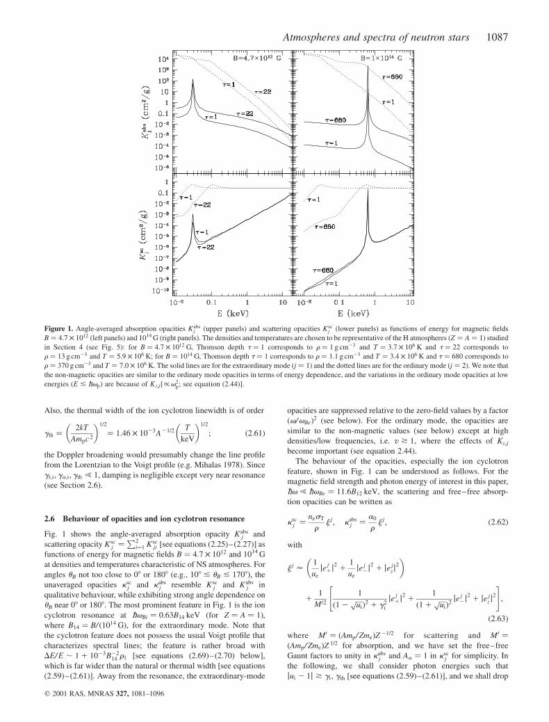
Fig. 1 shows the angle-averaged absorption opacity Kabsj and

scattering opacity Kscj ¼

P2i¼1 Ksc

ji [see equations (2.25)–(2.27)] as

functions of energy for magnetic fields B ¼ 4:7 � 1012 and 1014 G

at densities and temperatures characteristic of NS atmospheres. For

angles uB not too close to 08 or 1808 (e.g., 108 & uB & 1708Þ, the

unaveraged opacities kscj and kabs

j resemble Kscj and Kabs

j in

qualitative behaviour, while exhibiting strong angle dependence on

uB near 08 or 1808. The most prominent feature in Fig. 1 is the ion

cyclotron resonance at ÉvBi ¼ 0:63B14 keV (for Z ¼ A ¼ 1Þ,

where B14 ¼ B/ ð1014 GÞ, for the extraordinary mode. Note that

the cyclotron feature does not possess the usual Voigt profile that

characterizes spectral lines; the feature is rather broad with

DE/E , 1 1 1023B2214 r1 [see equations (2.69)–(2.70) below],

which is far wider than the natural or thermal width [see equations

(2.59)–(2.61)]. Away from the resonance, the extraordinary-mode

opacities are suppressed relative to the zero-field values by a factor

ðv/vBeÞ2 (see below). For the ordinary mode, the opacities are

similar to the non-magnetic values (see below) except at high

densities/low frequencies, i.e. v * 1, where the effects of Kz,j

become important (see equation 2.44).

The behaviour of the opacities, especially the ion cyclotron

feature, shown in Fig. 1 can be understood as follows. For the

magnetic field strength and photon energy of interest in this paper,

Év ! ÉvBe ¼ 11:6B12 keV, the scattering and free–free absorp-

tion opacities can be written as

kscj ¼

nesT

rj j; kabs

j ¼a0

rj j; ð2:62Þ

with

j j <1

ue

jej1j

21

1

ue

je j2j

21 je j

z j2

� �

11

M021

ð1 2ffiffiffiffiuipÞ2 1 g2

i

jej1j

21

1

ð1 1ffiffiffiffiuipÞ2je j

2j2

1 je jz j

2

" #;

ð2:63Þ

where M0 ¼ ðAmp/ZmeÞZ21=2 for scattering and M0 ¼

ðAmp/ZmeÞZ1=2 for absorption, and we have set the free–free

Gaunt factors to unity in kabsj and Aa ¼ 1 in ksc

j for simplicity. In

the following, we shall consider photon energies such that

jui 2 1j * gi, gth [see equations (2.59)–(2.61)], and we shall drop

Figure 1. Angle-averaged absorption opacities Kabsj (upper panels) and scattering opacities Ksc

j (lower panels) as functions of energy for magnetic fields

B ¼ 4:7 � 1012 (left panels) and 1014 G (right panels). The densities and temperatures are chosen to be representative of the H atmospheres ðZ ¼ A ¼ 1Þ studied

in Section 4 (see Fig. 5): for B ¼ 4:7 � 1012 G, Thomson depth t ¼ 1 corresponds to r ¼ 1 g cm23 and T ¼ 3:7 � 106 K and t ¼ 22 corresponds to

r ¼ 13 g cm23 and T ¼ 5:9 � 106 K; for B ¼ 1014 G, Thomson depth t ¼ 1 corresponds to r ¼ 1:1 g cm23 and T ¼ 3:4 � 106 K and t ¼ 680 corresponds to

r ¼ 370 g cm23 and T ¼ 7:0 � 106 K. The solid lines are for the extraordinary mode ðj ¼ 1Þ and the dotted lines are for the ordinary mode ðj ¼ 2Þ. We note that

the non-magnetic opacities are similar to the ordinary mode opacities in terms of energy dependence, and the variations in the ordinary mode opacities at low

energies ðE & ÉvpÞ are because of Kz;j½/v2p; see equation (2.44)].

Atmospheres and spectra of neutron stars 1087

q 2001 RAS, MNRAS 327, 1081–1096

the g2i term from equation (2.63). Also for simplicity, we shall set

Z ¼ A ¼ 1.

For uB not too small, i.e. sin2uB/cos uB , 1, the polarization

parameter b (see equation 2.45) satisfies jbj @ 1 except when v is

very close to the ion cyclotron resonance (i.e. j1 2 ui 2 ð1 1 vÞ/

Mj& u21=2e Þ or when Év & Év2

p/vBe ¼ 0:07r1B2112 eV. In the limit

of jbj @ 1, we find K1 ¼ 21=ð2bÞ and K2 ¼ 2b, and thus

je1^j

2¼

1

21 7

1

bcos uB

� �; je1

z j2¼

1

ð2bÞ2sin2uB; ð2:64Þ

je2^j

2¼

1

2cos2uB 1 ^

1

b cos uB

� �;

je2z j

2¼ 1 2

1

ð2bÞ2

� �sin2uB; ð2:65Þ

where, for simplicity, we have taken the transverse approximation

so that Kz;j < 0. Substituting these into equation (2.63), we obtain,

for jbj @ 1,

j 1 <1

ue

1 1ð1 2 vÞ2 cos2uB/ sin2uB 1 uið1 1 uiÞ

ð1 2 uiÞ2

� �; ð2:66Þ

and

j 2 < sin2uB 11

ue

� ðcos2uB 1 ui sin2uBÞ1 cos2uB

uið1 1 uiÞ2 ð1 2 vÞ2/sin2uB

ð1 2 uiÞ2

� �:

ð2:67Þ

Clearly, away from ion cyclotron resonance, j 1/u21e ¼ ðv/vBeÞ

2,

and thus the opacities for the extraordinary mode are suppressed

compared to the zero-field values:

ksc1 /

v

vBe

� �2

; kabs1 /

1

v2Bevð1 2 e2Év/kT Þ: ð2:68Þ

At high densities/low frequencies, such that v * 1, these are

multiplied by a term of order 1 1 Oðv 2Þ; for v @ 1, we have

ksc1 /v4

p/ ðv2Bev

2Þ. For the ordinary mode, j 2 , 1, and thus the

opacities are approximately unchanged from the zero-field values.

Equations (2.66) and (2.67) also apply to photon energies near

the ion cyclotron resonance as long as j1 2 uij @ ð1 1 vÞ/M, so

that jbj @ 1 (note that we are considering typical angles where

jcos uBj , 1Þ. It is evident from equation (2.66) that, for the

extraordinary mode, the opacities exhibit a broad peak/feature

around vBi, i.e. the term contained inside the brackets in equation

(2.66) becomes significantly greater than unity. The width of the

feature, j1 2 uij, is of order

Gi ;v 2 vBi

vBi

���� ���� < 2 1 ð1 2 v resÞ2cos2uB

sin2uB

� �1=2

; ð2:69Þ

where

v res ¼v2

p

v2Bi

<r

1 g cm23

� �B

4:6 � 1012 G

� �22

: ð2:70Þ

It is important to note that, although the natural and thermal width

of the ion cyclotron line are rather narrow [see equations (2.59)–

(2.61)], the cyclotron feature as described by equations (2.66) and

(2.69) is broad, i.e., the opacities are significantly affected by the

ion cyclotron resonance for 0:3 & v/vBi & 3. Also, equation

(2.67) indicates that, although the ion cyclotron resonance formally

occurs for the ordinary mode, its strength is diminished by the

ðv/vBeÞ2 ¼ ðme/mpÞ

2 suppression.

Finally, we note that the presence of ions induces a mode-

collapse point very near vBi. This can be seen from equation (2.45),

which shows that b ¼ 0 when 1 2 ui 2 ð1 1 vÞ/M ¼ 0 or

v ¼ vBi½1 1 ð1 1 vÞ=2M�. At this point, the two photon modes

become degenerate (both are circularly polarized), and the

transport equation (2.1) formally breaks down. This ion-induced

mode collapse is independent of the well-known mode collapse as

a result of vacuum polarization (Pavlov & Shibanov 1979; Ventura

et al. 1979; see Section 5). Note, however, that the ion-induced

mode-collapse feature is very narrow ½jbj ! 1 requires

j1 2 ui 2 ð1 1 vÞ/Mj ! u21=2e �, so it is completely ‘buried’ by

the much wider and more prominent ion cyclotron feature.

3 N U M E R I C A L M E T H O D

3.1 Magnetic atmospheres with full radiative transport

When presenting results of atmosphere models based on the full

transport equations, we consider only the case of B perpendicular

to the surface ðQB ¼ 08Þ. Thus the radiation intensity I jn depends on

depth t, energy E ¼ Év ¼ hn, and angle u.

We construct a grid in Thomson depth, energy, and angle with

intervals that are equally spaced logarithmically from 1024 to

,103 in depth and from 1022 to ,10 keV in energy and spaced

every 58 in angle. For typical calculations, six grid points are used

per decade in depth, 12 grid points are used per decade in energy,

and 19 total grid points in angle. We also increase the energy

resolution near the ion cyclotron resonance.

The temperature profile is initially assumed to be the grey

profile,

TðtRÞ ¼ Teff

3

4tR 1

2

3

� �� �1=4

: ð3:1Þ

The Rosseland mean depth tR is given by dtR ¼ ðkR/kes

0 Þ dt,

where the Rosseland mean opacity is

1

kR¼

3p

4sSBT 3

ð1

0

1

2 j

Xlj

›Bn

›Tdn ð3:2Þ

and lj is given by equation (2.23). Since lj and k R are functions of r

and T themselves, the profile (3.1) must be constructed by an

iterative process: the temperature profile is first taken to be

TðtÞ ¼ Teff½3=4ðt 1 2=3Þ�1=4; the density profile, and hence k tot and

k R, are then determined, which allows the calculation of tR(t);

using equation (3.1) with this tR, a revised temperature profile is

obtained; the process is repeated until the new tR(t) is not

significantly different from the previous tR(t). To achieve jDt/tj

and jDtR/tRj , 0:1 per cent, three iterations are required.

To construct self-consistent atmosphere models requires

successive global iterations, where the temperature profile T(t) is

adjusted from the previous iteration to satisfy radiative equi-

librium. At each global iteration, the profiles T(t) and r(t) are

considered fixed. We solve the RTE (2.8) [see also equations

(2.15)–(2.17)], together with the boundary conditions [see equa-

tions (2.9) and (2.10)] by the finite difference scheme described by

Mihalas (1978). This results in a set of equations which have the

form of a tridiagonal matrix that can be solved by the Feautrier

procedure of forward-elimination and back-substitution. We have

also implemented an improved Feautrier method to reduce errors

1088 W. C. G. Ho and D. Lai

q 2001 RAS, MNRAS 327, 1081–1096

arising from machine precision as suggested by Rybicki &

Hummer (1991). Note that, in the presence of scattering, the source

function S jn [which involves mode coupling; see equation (2.16)] is

not known prior to solving the RTE. We adopt the strategy that, for

each global iteration, S jn is calculated using the solution for i j

n from

the previous global iteration, with S jn ¼ Bn/2 for the first global

iteration. The full RTE is solved with this source function to obtain

i jn, and the specific flux is calculated from finite differencing

equation (2.7). Note that, unless the temperature correction from

the previous iteration is relatively small, so that the source function

calculated from the previous i jn approximates the true current

source function, the global iteration may not converge.2

The current solution i jn does not, in general, satisfy the radiative

equilibrium constraint nor does it yield a constant flux at every

depth [see equations (2.13) and (2.14), respectively]. To satisfy

both conditions requires correcting the temperature profile. We use

a variation of the Unsold–Lucy temperature correction method as

described by Mihalas (1978) but modified to account for full

radiative transfer by two propagation modes in a magnetic

medium. The radiative equilibrium constraint given by equation

(2.13) can be written as

dFz

dt¼ c

k J

kes0

u 2kP

kes0

u P

� �; ð3:3Þ

where u ¼P2

j¼1

Ðdn u j

n is the total radiation energy density, u P ¼

aT 4 ¼ ð4sSB/ cÞT 4 is the blackbody energy density, and k J and k P

are the absorption mean opacity and Planck mean opacity defined

by

k J ;2

cu

X2

j¼1

ðdn

ð1

dkkabsj ðkÞi

jnðkÞ; ð3:4Þ

kP ;1

4pu P

X2

j¼1

ðdn

ð1

dkkabsj ðkÞu

Pn ; ð3:5Þ

respectively. On the other hand, equation (2.7) can be integrated

out formally to give i jn in terms of f j

n, and we then have

cuðtÞ ¼ 2X2

j¼1

ðdn

ð1

dk i jnðtÞ

¼

ðt0

dt0kFðt0Þ

kes0

Fzðt0Þ1 2Fzð0Þ; ð3:6Þ

where we have used cuð0Þ < 2Fzð0Þ, Fz(t) is the total flux at depth

t (see equation 2.14), and k F(t) is the flux mean opacity defined by

kF ;2

Fz

X2

j¼1

ðdn

ð1

dk1

mktot

j ðkÞfjnðkÞ: ð3:7Þ

Combining equations (3.3) and (3.6) gives an expression for

u P[T(t)] in terms of Fz(t). The desired temperature correction

DT(t) needed to satisfy radiative equilibrium is then

DTðtÞ <1

16sSBTðtÞ32

k es0

kPðtÞ

d½DFzðtÞ�

dt1

k JðtÞ

kPðtÞ

�

�

ðt0

dt0kFðt0Þ

k es0

DFzðt0Þ1 2DFzð0Þ

� ��; ð3:8Þ

where DFzðtÞ ¼ sSBT4eff 2 FzðtÞ. Using equation (3.3) to replace

dFz/dt in equation (3.8), we obtain

DTðtÞ <1

16sSBTðtÞ3c

kPðtÞ½k JðtÞuðtÞ2 kPðtÞu PðtÞ�1

k JðtÞ

kPðtÞ

�

�

ðt0

dt0kFðt0Þ

k es0

DFzðt0Þ1 2DFzð0Þ

� ��: ð3:9Þ

Note that the first term in equation (3.9), which is /ðk Ju 2 kPu PÞ,

corresponds to the temperature correction in the L-iteration

procedure DTL ¼ ðkJu 2 kPu PÞð›u P/›TÞ21 and is important near

the surface but is small in the deeper layers where the atmosphere

approaches a blackbody, while the remaining terms provide

corrections in these deeper layers. In practice, we find that the

Unsold–Lucy temperature correction method as defined by

equation (3.9) tends to overcorrect; therefore we only use

,70–90 per cent of the temperature correction. The process of

determining the radiation intensity from the RTE for a given

temperature profile, estimating and applying the temperature

correction, and then recalculating the radiation intensity is repeated

until convergence of the solution is achieved. We note here that, to

decrease the number of iterations required for convergence and the

total computation time, we can use as the initial temperature profile

the result obtained from the diffusion calculation (see Section 3.2);

such an initial temperature profile would already be close to

radiative equilibrium.

Three criteria are used to indicate convergence. The first is that

the temperature correction between successive global iterations

becomes small, e.g., jDT/Tj & 1 per cent. The second is to check

that radiative equilibrium (see equation 2.13) is sufficiently

satisfied, or ðk Ju 2 kPu PÞ=ðk JuÞ is sufficiently small (see equation

3.3). The third criterion is that Fz is sufficiently close to sSBT4eff

(see equation 2.14). Fig. 2 shows an example of these convergence

tests after about 20 global iterations for our full radiative transport

model of a fully ionized, pure H atmosphere with Teff ¼ 5 � 106 K,

B ¼ 1014 G, and QB ¼ 08. Further iterations reduce the deviations,

although the convergence is slower since the temperature

corrections are already small. The numerical results presented

in Section 4 have all reached the convergence level similar to

Fig. 2.

3.2 Magnetic atmospheres with diffusion approximation

Using the diffusion approximation of radiative transport (see

Section 2.3), we construct magnetic atmosphere models for general

QB. We follow a similar procedure as the full radiative transfer

method described in Section 3.1. We solve the approximate RTE

(2.24) with boundary conditions given by equations (2.28) and

(2.29) using the Feautrier method, which involves only depth and

photon energy grid points. The modified Unsold–Lucy tempera-

ture correction can be derived using the specific flux perpendicular

to the stellar surface, F jn;z < 2cljð›u j

n/›zÞ, and equation (2.30). The

resulting DT(t) takes the same form as in equations (3.8) and (3.9),

2 An alternative is to calculate S jn iteratively within each global iteration.

The source function during each global iteration is first taken to be

S jn ¼ Bn/2, and thus the two modes are initially decoupled. The RTE is then

solved for each mode j. The resulting i jn is used to determine a revised

source function, which can then be reinserted into the RTE. This procedure

is repeated until the the source function converges, e.g. jDS jn/ S j

nj , 5 per

cent. Obviously, this method requires longer computation time. In addition,

we have implemented a procedure that reformulates the RTE using

Eddington factors (see, e.g., Rybicki & Lightman 1979 for the analogous

non-magnetic RTE using Eddington factors), but this does not lead to

significant reduction in computation time.

Atmospheres and spectra of neutron stars 1089

q 2001 RAS, MNRAS 327, 1081–1096

except that the mean opacities k J, k P, and k F are given by

k J ;1

u

X2

j¼1

ðdnKabs

j u jn; ð3:10Þ

kP ;1

2u P

X2

j¼1

ðdnKabs

j uPn ; ð3:11Þ

and

kF ;1

Fz

X2

j¼1

ðdn

1

rljF jn; ð3:12Þ

respectively. The expressions for k J and k P are essentially the

same as in Section 3.1. Atmosphere models for B & 1013 G based

on the diffusion approximation have been constructed by Shibanov

et al. (1992) and Pavlov et al. (1995) using a different iteration

scheme, i.e. L-iteration.

3.3 Non-magnetic atmospheres

For comparison, we also construct non-magnetic atmosphere

models by solving the standard RTE (both full transport and in the

diffusion approximation) using a similar method as described in

Sections 3.1 and 3.2. In this case, the opacities are just due to non-

magnetic electron scattering and free–free absorption. We

implement the RTE with Eddington factors to determine the

source function more accurately. We use the standard Feautrier

method (with improvements described by Rybicki & Hummer

1991) and the standard Unsold–Lucy temperature correction

scheme described by Mihalas (1978).

4 N U M E R I C A L R E S U LT S

4.1 Atmosphere structure

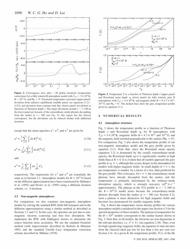
Fig. 3 shows the temperature profile as a function of Thomson

depth t and Rosseland depth tR for H atmospheres with

Teff ¼ 5 � 106 K, magnetic fields B ¼ 4:7 � 1012 and 1014 G, and

the magnetic field oriented perpendicular to the surface ðQB ¼ 08Þ.

For comparison, Fig. 3 also shows the temperature profile of our

non-magnetic atmosphere model and the grey profile given by

equation (3.1). Note that, since the Rosseland mean opacity

(equation 3.2) is dominated by the (small) extraordinary-mode

opacity, the Rosseland depth tR(t) is significantly smaller at high

fields than at B ¼ 0. It is evident that all models approach the grey

profile at tR @ 1, although this occurs deeper in the atmosphere for

models with higher magnetic fields. At small depths of t & 1, the

gas temperature is smaller, by a factor of a few, than predicted by

the grey profile. This is because, for t & 1, the extraordinary-mode

photons have already decoupled from the matter, and the

temperature is primarily determined by the ordinary-mode

absorption opacity, which is strongly non-grey ðkabs2 /n23

approximately). The plateau in the T(t) profile at t , 1–100 in

the B ¼ 1014 G model arises because the extraordinary-mode

photons decouple from the matter at t , 100 (see Section 4.2);

such a plateau is more distinctive for high magnetic fields and

becomes less pronounced for smaller magnetic fields.

Fig. 4 shows the temperature versus density profiles for various

atmosphere models considered in this paper (see Section 4.3 for the

spectral properties of these models). The plateau in temperature for

the B ¼ 1014 models corresponds to the similar feature shown in

Fig. 3. Note that, in all models, the electrons are non-degenerate at

the relevant densities, i.e., T @ TF (see equation 2.38). Thus, even

for high (quantizing) magnetic fields, the equation of state deviates

from the classical ideal gas law by less than a few per cent (see

Section 2.4). At a given B, the temperature profile, T(t), of the He

Figure 2. Convergence tests after , 20 global iterations (temperature

corrections) for a fully ionized H atmosphere model with Teff ¼ 5 � 106 K,

B ¼ 1014 G, and QB ¼ 08. Fractional temperature correction (upper panel),

deviation from radiative equilibrium [middle panel; see equations (3.3)–

(3.5)], and deviation from constant total flux (lower panel) are plotted as

functions of Thomson depth t. The larger deviations around t , 1–100 in

the lower panel are because of the extraordinary-mode photons decoupling

from the matter at t , 100 (see Fig. 5); this region has the slowest

convergence, but the deviations can be reduced further with additional

iterations.

Figure 3. Temperature T as a function of Thomson depth t (upper panel)

and Rosseland mean depth tR (lower panel) for fully ionized, pure H

atmospheres with Teff ¼ 5 � 106 K, and magnetic fields B ¼ 0; 4:7 � 1012,

1014 G and QB ¼ 08. The dashed lines show the grey temperature profile

given by equation (3.1).

1090 W. C. G. Ho and D. Lai

q 2001 RAS, MNRAS 327, 1081–1096

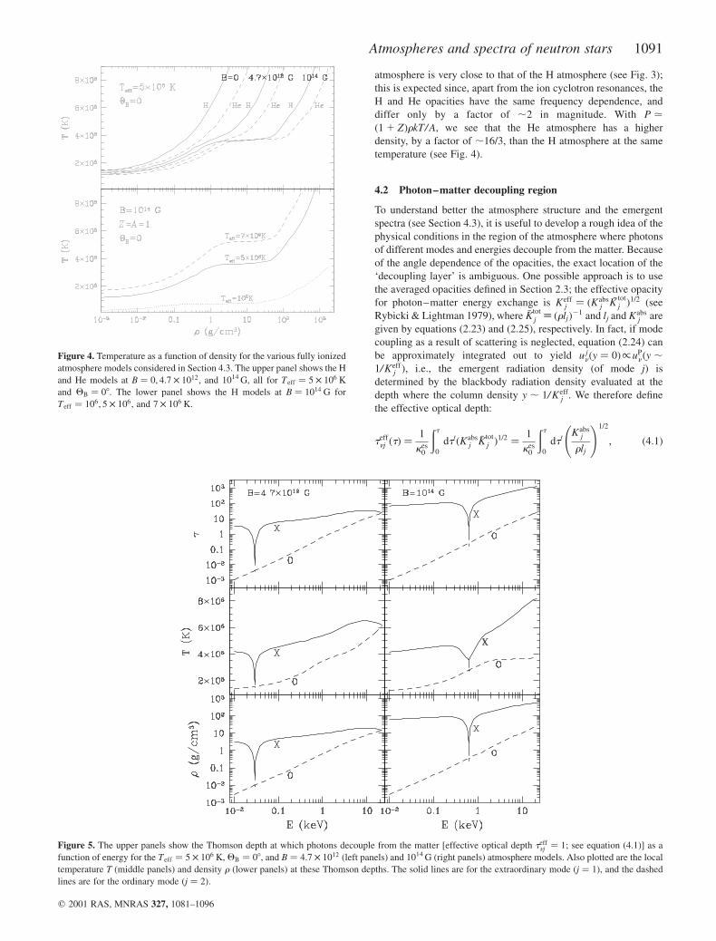
atmosphere is very close to that of the H atmosphere (see Fig. 3);

this is expected since, apart from the ion cyclotron resonances, the

H and He opacities have the same frequency dependence, and

differ only by a factor of ,2 in magnitude. With P .ð1 1 ZÞrkT/A; we see that the He atmosphere has a higher

density, by a factor of ,16/3, than the H atmosphere at the same

temperature (see Fig. 4).

4.2 Photon–matter decoupling region

To understand better the atmosphere structure and the emergent

spectra (see Section 4.3), it is useful to develop a rough idea of the

physical conditions in the region of the atmosphere where photons

of different modes and energies decouple from the matter. Because

of the angle dependence of the opacities, the exact location of the

‘decoupling layer’ is ambiguous. One possible approach is to use

the averaged opacities defined in Section 2.3; the effective opacity

for photon–matter energy exchange is Keffj ¼ ðK

absj

�Ktotj Þ

1=2 (see

Rybicki & Lightman 1979), where �Ktotj ; ðrljÞ

21 and lj and Kabsj are

given by equations (2.23) and (2.25), respectively. In fact, if mode

coupling as a result of scattering is neglected, equation (2.24) can

be approximately integrated out to yield u jnðy ¼ 0Þ/uP

nðy ,1/Keff

j Þ; i.e., the emergent radiation density (of mode j) is

determined by the blackbody radiation density evaluated at the

depth where the column density y , 1/Keffj . We therefore define

the effective optical depth:

teffnj ðtÞ ¼

1

kes0

ðt0

dt0ðKabsj

�Ktotj Þ

1=2 ¼1

kes0

ðt0

dt0Kabs

j

rlj

!1=2

; ð4:1Þ

Figure 4. Temperature as a function of density for the various fully ionized

atmosphere models considered in Section 4.3. The upper panel shows the H

and He models at B ¼ 0; 4:7 � 1012, and 1014 G, all for Teff ¼ 5 � 106 K

and QB ¼ 08. The lower panel shows the H models at B ¼ 1014 G for

Teff ¼ 106; 5 � 106, and 7 � 106 K.

Figure 5. The upper panels show the Thomson depth at which photons decouple from the matter [effective optical depth teffnj ¼ 1; see equation (4.1)] as a

function of energy for the Teff ¼ 5 � 106 K, QB ¼ 08, and B ¼ 4:7 � 1012 (left panels) and 1014 G (right panels) atmosphere models. Also plotted are the local

temperature T (middle panels) and density r (lower panels) at these Thomson depths. The solid lines are for the extraordinary mode ðj ¼ 1Þ, and the dashed

lines are for the ordinary mode ðj ¼ 2Þ.

Atmospheres and spectra of neutron stars 1091

q 2001 RAS, MNRAS 327, 1081–1096

so that photons of mode j and frequency n decouple from the

matter at teffnj , 1. Fig. 5 shows the Thomson depth and local

temperature and density as functions of photon energy at the

decoupling layer for the H atmosphere model with Teff ¼

5 � 106 K; QB ¼ 08, and B ¼ 4:7 � 1012 and 1014 G (see also

Fig. 3). Note that the effective depth defined in equation (4.1) errs

for photons propagating along the magnetic field since the

opacities are generally lower near uB ¼ 0; hence, these photons

decouple from the matter at deeper layers than those indicated in

Fig. 5. Nevertheless, Fig. 5 gives the typical conditions where the

observed photons of energy E are generated. It is clear that the

extraordinary-mode photons can emerge from deep in the atmos-

phere where plasma effects on the opacities are not negligible (see

Section 2.5 and Fig. 1). Photons with energies near the ion

cyclotron resonance EBi ¼ 0:63B14 keV decouple in the lower

temperature region; this gives rise to the absorption feature in the

emergent radiation spectrum (see Section 4.3).

4.3 Spectra

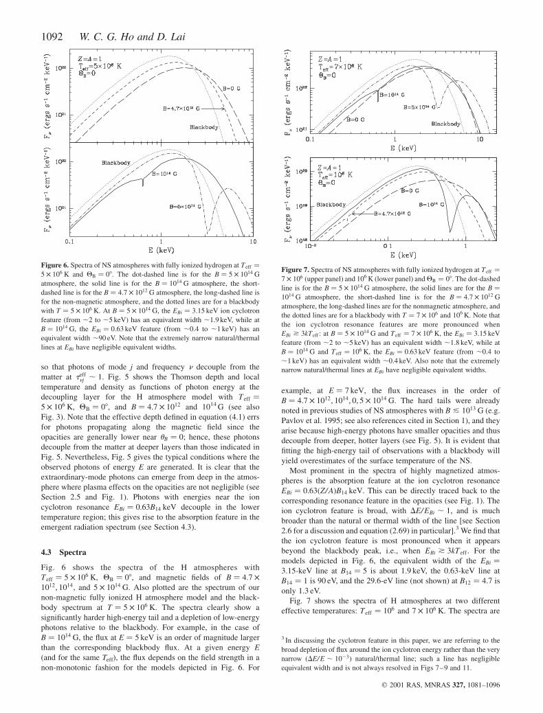
Fig. 6 shows the spectra of the H atmospheres with

Teff ¼ 5 � 106 K, QB ¼ 08, and magnetic fields of B ¼ 4:7 �

1012; 1014; and 5 � 1014 G. Also plotted are the spectrum of our

non-magnetic fully ionized H atmosphere model and the black-

body spectrum at T ¼ 5 � 106 K. The spectra clearly show a

significantly harder high-energy tail and a depletion of low-energy

photons relative to the blackbody. For example, in the case of

B ¼ 1014 G, the flux at E ¼ 5 keV is an order of magnitude larger

than the corresponding blackbody flux. At a given energy E

(and for the same Teff), the flux depends on the field strength in a

non-monotonic fashion for the models depicted in Fig. 6. For

example, at E ¼ 7 keV, the flux increases in the order of

B ¼ 4:7 � 1012; 1014; 0; 5 � 1014 G. The hard tails were already

noted in previous studies of NS atmospheres with B & 1013 G (e.g.

Pavlov et al. 1995; see also references cited in Section 1), and they

arise because high-energy photons have smaller opacities and thus

decouple from deeper, hotter layers (see Fig. 5). It is evident that

fitting the high-energy tail of observations with a blackbody will

yield overestimates of the surface temperature of the NS.

Most prominent in the spectra of highly magnetized atmos-

pheres is the absorption feature at the ion cyclotron resonance

EBi ¼ 0:63ðZ/AÞB14 keV. This can be directly traced back to the

corresponding resonance feature in the opacities (see Fig. 1). The

ion cyclotron feature is broad, with DE/EBi , 1, and is much

broader than the natural or thermal width of the line [see Section

2.6 for a discussion and equation (2.69) in particular].3 We find that

the ion cyclotron feature is most pronounced when it appears

beyond the blackbody peak, i.e., when EBi * 3kTeff . For the

models depicted in Fig. 6, the equivalent width of the EBi ¼

3:15-keV line at B14 ¼ 5 is about 1.9 keV, the 0.63-keV line at

B14 ¼ 1 is 90 eV, and the 29.6-eV line (not shown) at B12 ¼ 4:7 is

only 1.3 eV.

Fig. 7 shows the spectra of H atmospheres at two different

effective temperatures: Teff ¼ 106 and 7 � 106 K. The spectra are

Figure 7. Spectra of NS atmospheres with fully ionized hydrogen at Teff ¼

7 � 106 (upper panel) and 106 K (lower panel) and QB ¼ 08. The dot-dashed

line is for the B ¼ 5 � 1014 G atmosphere, the solid lines are for the B ¼

1014 G atmosphere, the short-dashed line is for the B ¼ 4:7 � 1012 G

atmosphere, the long-dashed lines are for the nonmagnetic atmosphere, and

the dotted lines are for a blackbody with T ¼ 7 � 106 and 106 K. Note that

the ion cyclotron resonance features are more pronounced when

EBi * 3kTeff : at B ¼ 5 � 1014 G and Teff ¼ 7 � 106 K, the EBi ¼ 3:15 keV

feature (from ,2 to ,5 keV) has an equivalent width ,1.8 keV, while at

B ¼ 1014 G and Teff ¼ 106 K, the EBi ¼ 0:63 keV feature (from ,0.4 to

,1 keV) has an equivalent width ,0.4 keV. Also note that the extremely

narrow natural/thermal lines at EBi have negligible equivalent widths.

Figure 6. Spectra of NS atmospheres with fully ionized hydrogen at Teff ¼

5 � 106 K and QB ¼ 08. The dot-dashed line is for the B ¼ 5 � 1014 G

atmosphere, the solid line is for the B ¼ 1014 G atmosphere, the short-

dashed line is for the B ¼ 4:7 � 1012 G atmosphere, the long-dashed line is

for the non-magnetic atmosphere, and the dotted lines are for a blackbody

with T ¼ 5 � 106 K. At B ¼ 5 � 1014 G, the EBi ¼ 3:15 keV ion cyclotron

feature (from ,2 to ,5 keV) has an equivalent width ,1.9 keV, while at

B ¼ 1014 G, the EBi ¼ 0:63 keV feature (from ,0.4 to ,1 keV) has an

equivalent width ,90 eV. Note that the extremely narrow natural/thermal

lines at EBi have negligible equivalent widths.

3 In discussing the cyclotron feature in this paper, we are referring to the

broad depletion of flux around the ion cyclotron energy rather than the very

narrow ðDE/E , 1023Þ natural/thermal line; such a line has negligible

equivalent width and is not always resolved in Figs 7–9 and 11.

1092 W. C. G. Ho and D. Lai

q 2001 RAS, MNRAS 327, 1081–1096

similar to those of the Teff ¼ 5 � 106 K models shown in Fig. 6.

The cyclotron resonance at 0.63 keV (for B14 ¼ 1Þ becomes

prominent for Teff ¼ 106 K since the condition EBi * 3kTeff is

satisfied. Note that the Teff ¼ 106 K models should be considered

for illustrative purposes only since we expect the opacities to be

significantly modified by neutral atoms and even molecules at such

a low temperature (see Section 5).

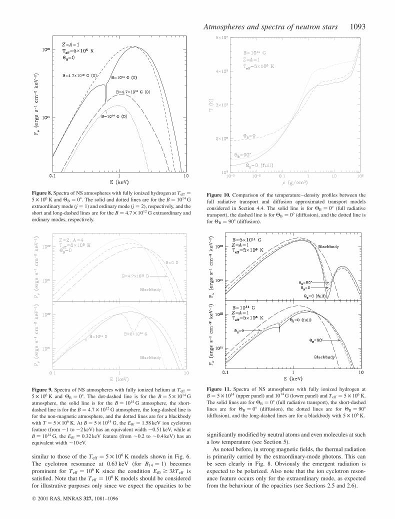
As noted before, in strong magnetic fields, the thermal radiation

is primarily carried by the extraordinary-mode photons. This can

be seen clearly in Fig. 8. Obviously the emergent radiation is

expected to be polarized. Also note that the ion cyclotron reson-

ance feature occurs only for the extraordinary mode, as expected

from the behaviour of the opacities (see Sections 2.5 and 2.6).

Figure 10. Comparison of the temperature–density profiles between the

full radiative transport and diffusion approximated transport models

considered in Section 4.4. The solid line is for QB ¼ 08 (full radiative

transport), the dashed line is for QB ¼ 08 (diffusion), and the dotted line is

for QB ¼ 908 (diffusion).

Figure 9. Spectra of NS atmospheres with fully ionized helium at Teff ¼

5 � 106 K and QB ¼ 08. The dot-dashed line is for the B ¼ 5 � 1014 G

atmosphere, the solid line is for the B ¼ 1014 G atmosphere, the short-

dashed line is for the B ¼ 4:7 � 1012 G atmosphere, the long-dashed line is

for the non-magnetic atmosphere, and the dotted lines are for a blackbody

with T ¼ 5 � 106 K. At B ¼ 5 � 1014 G, the EBi ¼ 1:58 keV ion cyclotron

feature (from ,1 to ,2 keV) has an equivalent width ,0.51 keV, while at

B ¼ 1014 G, the EBi ¼ 0:32 keV feature (from ,0.2 to ,0.4 keV) has an

equivalent width ,10 eV.

Figure 8. Spectra of NS atmospheres with fully ionized hydrogen at Teff ¼

5 � 106 K and QB ¼ 08. The solid and dotted lines are for the B ¼ 1014 G

extraordinary mode ðj ¼ 1Þ and ordinary mode ðj ¼ 2Þ, respectively, and the

short and long-dashed lines are for the B ¼ 4:7 � 1012 G extraordinary and

ordinary modes, respectively.

Figure 11. Spectra of NS atmospheres with fully ionized hydrogen at

B ¼ 5 � 1014 (upper panel) and 1014 G (lower panel) and Teff ¼ 5 � 106 K.

The solid lines are for QB ¼ 08 (full radiative transport), the short-dashed

lines are for QB ¼ 08 (diffusion), the dotted lines are for QB ¼ 908

(diffusion), and the long-dashed lines are for a blackbody with 5 � 106 K.

Atmospheres and spectra of neutron stars 1093

q 2001 RAS, MNRAS 327, 1081–1096

Fig. 9 shows the spectra of the He atmospheres with

Teff ¼ 5 � 106 K, QB ¼ 08, and magnetic fields of B ¼ 0; 4:7 �

1012; 1014 and 5 � 1014 G. These should be compared to the spectra

of H atmospheres shown in Fig. 6. Although the He atmosphere is

denser than the H atmosphere (see Section 4.1 and Fig. 4), there is

no clear distinction between their spectra except for the ion

cyclotron resonance features. For example, at B ¼ 1014 G and

Teff ¼ 5 � 106 K, the flux of the He atmosphere at E ¼ 6 keV is

lower than that of the H atmosphere by only a factor of 1.2. Clearly,

it would be difficult to distinguish a H atmosphere from a He

atmosphere based on spectral information in the 1–10 2 keV band

alone. We also note that the equivalent widths of the ion cyclotron

features for the He atmospheres are about 0.51 keV for the EBi ¼

1:58-keV line at B14 ¼ 5 and about 10 eV for the EBi ¼ 0:32-keV

line at B14 ¼ 1.

4.4 Full radiative transport versus diffusion approximation

The atmosphere models presented in Sections 4.1–4.3 are based on

solutions of the full RTEs (see Sections 2.1 and 3.1). These models

are currently restricted to the case where the magnetic field is

perpendicular to the stellar surface, i.e. QB ¼ 08. Using the

diffusion approximation (see Sections 2.3 and 3.2), we construct

atmosphere models for general QBs.

Fig. 10 shows the temperature–density profiles of the H

atmosphere models with B ¼ 1014 G, Teff ¼ 5 � 106 K, and QB ¼

08 and 908 based on the diffusion approximation. These are

compared with the result of the corresponding full transport model

with QB ¼ 08. Clearly, in the diffusion models, the surface

temperature (where r & 0:01 g cm23Þ for QB ¼ 908 is significantly

less than for QB ¼ 08 (by roughly a factor of 1.4 for the models

considered here); this was already noted by Pavlov et al. (1995) and

Shibanov et al. (1992) for the B , 1012 G models. At 1014 G, the

temperature plateaus (as a result of the decoupling of the

extraordinary-mode photons; see Section 4.1) are also different for

QB ¼ 08 and 908. The difference in the temperature profiles for

different magnetic field geometries implies that different parts of

the NS surface will have different temperatures, e.g., the magnetic

equator is cooler than the magnetic poles, even if Teff is uniform.

Clearly, a full understanding of the NS surface temperature

distribution requires detailed modelling of the three-dimensional

atmosphere and of the anisotropic heat transport through the NS

crust; this is beyond the scope of this paper. Comparing the

diffusion model with the full transport model, we see from Fig. 10

that, at QB ¼ 08, the temperature in the full model is significantly

lower than that of the diffusion model in the outermost layers of the

atmosphere.

Fig. 11 shows that, despite the difference in the temperature

profiles, the spectra of the diffusion models for QB ¼ 08 and 908

and the spectra of the full transport model are rather similar. For

B14 ¼ 1, the equivalent width of the cyclotron feature at EBi ¼

0:63 keV is about 80 eV for QB ¼ 08 and 50 eV for QB ¼ 908,

while for B14 ¼ 5, the feature at EBi ¼ 3:15 keV has a width of

about 1.9 keV for QB ¼ 08 and 908. We also find that the polarized

emission is stronger for QB ¼ 908 than for 08, as already noted by

Shibanov et al. (1992) for the B ¼ 4:7 � 1012 G models.

5 D I S C U S S I O N

In this paper, we have constructed models of magnetized NS

atmospheres composed of ionized hydrogen or helium. We focused

on the superstrong field regime ðB * 1014 GÞ as directly relevant to

magnetars (see Section 1). We solve the full, angle-dependent

RTEs for the coupled polarization modes and include the ion

cyclotron and plasma effects on the opacities and polarization

modes. Since the magnetic field greatly suppresses the opacities of

the extraordinary-mode photons, the thermal radiation emerges

from deep in the atmosphere ðr , 102 g cm23 for B ¼ 1014 GÞ,

where the medium effect is non-negligible. As already noted in

previous works on NS atmospheres with moderate (,1012 G) or

negligible magnetic fields, the thermal emission from a highly

magnetized NS is polarized, with the spectrum harder than the

blackbody. We find that the ion cyclotron resonance, at

EBi ¼ 0:63ðZ/AÞðB/1014 GÞ keV, can give rise to a broad

(DE/E , 1Þ and potentially observable absorption feature in the

spectrum, especially when EBi * 3kTeff . Clearly the detection of

such a feature would provide an important diagnostic for

magnetars.

We note that the spectra presented in this paper (see Figs 6–9

and 11) correspond to emission from a local patch of the NS

surface. To compare directly with observations, one must calculate

synthetic spectra from the whole stellar surface, taking into

account the effect of gravitational redshift and light-bending. To do

this, one must know the distribution of the magnetic field (both

magnitude and direction) and the effective temperature over the

stellar surface. For a given field geometry, the surface temperature

distribution may be obtained from crustal heat conduction

calculations (e.g. Hernquist 1985; Schaaf 1990; Page 1995; Heyl

& Hernquist 1998), but this is intrinsically coupled to the

properties of the atmosphere; the problem is further complicated by

the existence of lateral radiative flux (see Section 2.3) and the non-

uniform temperature distribution induced by the magnetic field in

the atmosphere (see Section 4.4). Obviously we expect the

cyclotron feature to be broadened and less deep if different parts of

the surface with different field strengths contribute similarly to the

observed flux (see Zane et al. 2001 for a calculation based on a

dipole field and an approximate temperature distribution).

Several physical effects have been neglected in our atmosphere

models (see Ozel 2001; Zane et al. 2001, for related works on

magnetar atmospheres; see also Section 1 for references of

previous works). We have assumed that the atmosphere is fully

ionized. The problem of ionization equilibrium in a highly

magnetized medium is a complicated one owing to the non-trivial

coupling between the centre-of-mass motion and the internal

atomic structure and to the relatively high densities of the

atmosphere (see Lai 2001 and references therein). While estimates

based on the calculations of Potekhin et al. (1999) indicate that the

fraction of neutral atoms is no more than a few per cent for T *

5 � 106 K at B , 1014 G, it should be noted that even a small

neutral fraction can potentially affect the radiative opacities. For

example, the ionization edge of a stationary H atom (in the ground

state) occurs at energy Ei < 4:4ðln bÞ2 eV, where b ; B/ ð2:35 �

109 GÞ (thus, Ei ¼ 0:16, 0.31, 0.54, 0.87 keV for B ¼ 1012, 1013,

1014, 1015 G, respectively; see Lai 2001). The ratio of the free–free

and bound-free opacities (for the extraordinary mode) at E ¼ Ei is

of order 1026r1/ ðT1=26 B14 f HÞ, where r1 ¼ r/ ð1 g cm23Þ, T6 ¼

T/ ð106 KÞ; B14 ¼ B/ ð1014 GÞ, and fH is the fraction of H atoms in

the ‘centred’ ground state (see Lai 2001). Thus one could in

principle expect atomic features, broadened by the ‘motional Stark

effect,’ in the spectra; these could blend with the ion cyclotron

feature, at EBi, studied in this paper.

Another caveat of our models is the neglect of the vacuum

polarization effect. In a strong magnetic field, vacuum polarization

(in which photons are temporarily converted into electron–positron

1094 W. C. G. Ho and D. Lai

q 2001 RAS, MNRAS 327, 1081–1096

pairs) contributes to the refractive index by a term of order

dvp ¼ ðaF/45pÞðB/BQÞ2, where aF ¼ 1=137 and BQ ¼

4:4 � 1013 G; and the effect tends to induce linear polarization of

the modes (Adler 1971). Thus for 3dvp * ðvp/vÞ2 (where vp is the

electron plasma frequency), or, for photon energies

Év * Évvp ¼ ð15p/aFÞ1=2ðvp/vBeÞmec 2 ¼ 1:0r1=2

1 B2114 keV,4 the

normal modes (and thus the radiative opacities) are modified by

vacuum polarization (e.g. Gnedin, Pavlov & Shibanov 1978;

Meszaros & Ventura 1979). Previous works (see Meszaros 1992 for

a review; see also Shibanov et al. 1992; Ozel 2001 for atmosphere

models that include the vacuum polarization effect; note that Ozel

2001 studied the B @ BQ regime but used the vacuum polarization

expressions valid only for B ! BQÞ neglected the response of the

ions in calculating the dielectric tensor. However, as shown in this

paper, for B * 1014 G, the ion cyclotron resonance gives rise to a

prominent feature in the polarization mode vector and in the

opacities. Therefore one must consider the combined system of

electrons, ions, and polarized vacuum in order to model the spectra

in the superstrong field regime (Ho & Lai, in preparation). Also,

vacuum polarization causes the opacities to exhibit a resonance

feature at E ¼ Évvp (Pavlov & Shibanov 1979; Ventura et al. 1979;

see Meszaros 1992 for a review). Since Évvp/r 1=2 and since

atmosphere models necessarily require discrete depth (density) and

energy grid points, such features can appear in the model spectra,

while, in a real atmosphere, they will be smoothed out. Moreover,

vacuum polarization can induce resonant mode conversion which

may significantly affect the radiation transport (Lai & Ho 2001).

We will present atmosphere models including vacuum polarization

in a future work (Ho & Lai, in preparation).

Finally, although in this paper we have included the medium

effect on the polarization modes (see Section 2.5), at sufficiently

high densities or low photon energies, the refractive index of the

medium deviates from unity or even becomes complex. This will

introduce additional effects on the radiative transport and the

resulting spectra. This issue will be addressed in a future work.

AC K N OW L E D G M E N T S

We would like to express our appreciation to Roberto Turolla for

his careful reading of the manuscript and his suggestions and

comments. DL thanks Feryal Ozel for discussions of her work at

the ITP conference ‘Spin and Magnetism in Young Neutron Stars’

held in 2000 October. This work was supported in part by NASA

Grant NAG 5-8484 and NAG 5-8356 and NSF grant AST 9986740.

DL was also supported by a fellowship from the A.P. Sloan

foundation.

R E F E R E N C E S

Adler S. L., 1971, Ann. Phys., 67, 599

Alcock C., Illarionov A., 1980, ApJ, 235, 534

Alpar M. A., 2001, ApJ, 554, 1245

Antia H. M., 1993, ApJS, 84, 101

Becker W., 2000, in Martens P. C. H., Tsuruta S., Weber M. A., eds, Proc.

IAU Symp. 195, Highly Energetic Physical Processes and Mechanisms

for Emission from Astrophysical Plasmas. Astron. Soc. Pac., San

Francisco, p. 49

Becker W., Trumper J., 1997, A&A, 326, 682

Bulik T., Pavlov G. G., 1996, ApJ, 469, 373

Caraveo P. A., 1998, Advances in Space Research, 21, 187

Caraveo P. A., Bignami G. F., Trumper J., 1996, A&AR, 7, 209

Caraveo P. A., Mignani R. P., Pavlov G. G., Bignami G. F., 2000, Proc. A

Decade of HST Science. Baltimore, in press (astro-ph/0008523)

Chatterjee P., Hernquist L., Narayan R., 2000, ApJ, 534, 373

Duncan R. C., Thompson C., 1992, ApJ, 392, L9

Edelstein J., Foster R. S., Bowyer S., 1995, ApJ, 454, 442

Ginzburg V. L., 1970, Propagation of Electromagnetic Waves in Plasmas.

2nd edn. Pergamon Press, Oxford

Gnedin Yu. N., Pavlov G. G., 1974, Sov. Phys. JETP, 38, 903

Gnedin Yu. N., Pavlov G. G., Shibanov Yu. A., 1978, Sov. Astron. Lett., 4,

117

Hernquist L., 1985, MNRAS, 213, 313

Heyl J. S., Hernquist L., 1997a, ApJ, 489, L67

Heyl J. S., Hernquist L., 1997b, J. Phys. A, 30, 6485

Heyl J. S., Hernquist L., 1998, MNRAS, 300, 599

Hulleman F., van Kerkwijk M. H., Kulkarni S. R., 2000, Nat, 408, 689

Hurley K., 2000, in Kippen R. M., Mallozzi R. S., Fishman G. J., eds,

Gamma-Ray Bursts: Fifth Huntsville Symposium, AIP Conf. Proc. 526.

Am. Inst. Phys., New York

Kaminker A. D., Pavlov G. G., Shibanov Yu. A., 1982, Ap&SS, 86, 249

Kaminker A. D., Pavlov G. G., Shibanov Yu. A., 1983, Ap&SS, 91, 167

Kaplan D. L., Kulkarni S. R., van Kerkwijk M. H., Rothschild R. E.,

Lingenfelter R. L., Marsden D., Danner R., Murakami T., 2001, ApJ,

556, 399

Kaspi V. M., Gavriil F. P., Chakrabarty D., Lackey J. R., Muno M. P., 2001,

ApJ, in press (astro-ph/0011368)

Korpela E. J., Bowyer S., 1998, AJ, 115, 2551

Kouveliotou C. et al., 1998, Nat, 393, 235

Kouveliotou C. et al., 1999, ApJ, 510, L115

Lai D., 2001, Rev. Mod. Phys., 73, in press (astro-ph/0009333)

Lai D., Ho W. C. G., 2001, ApJL, submitted (astro-ph/0108127)

Lai D., Salpeter E. E., 1997, ApJ, 491, 270

Mereghetti S., 1999, review presented at NATO ASI ‘Neutron Star-Black

Hole Connection’ (astro-ph/9911252)

Meszaros P., 1992, High-Energy Radiation from Magnetized Neutron Stars.

Univ. Chicago Press, Chicago

Meszaros P., Ventura J., 1979, Phys. Rev. D, 19, 3565

Meyer R. D., Pavlov G. G., Meszaros P., 1994, ApJ, 433, 265

Mignani R., Caraveo P. A., Bignami G. E., 1998, Advances in Space

Research, 21, 197

Mihalas D., 1978, Stellar Atmospheres. 2nd edn. W.H. Freeman and Co.,

San Francisco

Miller M. C., 1992, MNRAS, 255, 129

Nagel W., 1980, ApJ, 236, 904

Nagel W., Ventura J., 1983, A&A, 118, 66

Ozel F., 2001, ApJ, submitted (astro-ph/0103227)

Paerels F. et al., 2001, A&A, 365, L298

Page D., 1995, Space Sci. Rev., 74, 437

Pavlov G., 2000, http://online.itp.ucsb.edu/online/neustars_c00/pavlov/

Pavlov G. G., Panov A. N., 1976, Sov. Phys. JETP, 44, 300

Pavlov G. G., Shibanov Yu. A., 1979, Sov. Phys. JETP, 49, 741

Pavlov G. G., Zavlin V. E., 2000, ApJ, 529, 1011

Pavlov G. G., Shibanov Yu. A., Ventura J., Zavlin V. E., 1994, A&A, 289,

837

Pavlov G. G., Shibanov Yu. A., Zavlin V. E., Meyer R. D., 1995, in Alpar

M. A., Kiziloglu U., van Paradijs J., eds, Lives of the Neutron Stars.

Kluwer Academic, Boston, p. 71

Pavlov G. G., Zavlin V. E., Trumper J., Neuhauser R., 1996, ApJ, 472,

L33

Pavlov G. G., Welty A. D., Cordova F. A., 1997, ApJ, 489, L75

Perna R., Heyl J. S., Hernquist L. E., Juett A. M., Chakrabarty D., 2001,

ApJ, 557, 18

Potekhin A. Y., Chabrier G., Shibanov Yu. A., 1999, Phys. Rev. E, 60,

2193

Rajagopal M., Romani R. W., 1996, ApJ, 461, 327

Rajagopal M., Romani R. W., Miller M. C., 1997, ApJ, 479, 347

4 The expressions of dvp and Évvp given here are valid for B ! BQ. The use

of more general expressions (Tsai & Erber 1975; Heyl & Hernquist 1997b)

results in different scalings with B, and the numerical values differ by a

factor of a few for B , 1014–1015 G (Ho & Lai, in preparation).

Atmospheres and spectra of neutron stars 1095

q 2001 RAS, MNRAS 327, 1081–1096

Romani R. W., 1987, ApJ, 313, 718

Rybicki G. B., Hummer D. G., 1991, A&A, 245, 171

Rybicki G. B., Lightman A. P., 1979, Radiative Processes in Astrophysics.

John Wiley & Sons, New York

Schaaf M. E., 1990, A&A, 227, 61

Shafranov V. D., , Leontovich M. A. 1967, Reviews of Plasma Physics,

Vol. 3. Consultants Bureau, New York

Shapiro S. L., Teukolsky S. A., 1983, Black Holes, White Dwarfs, and

Neutron Stars. John Wiley & Sons, New York

Shibanov Yu. A., Zavlin V. E., 1995, Astron. Lett., 21, 3

Shibanov Yu. A., Zavlin V. E., Pavlov G. G., Ventura J., 1992, A&A, 266,

313

Thompson C., 2000, in Connaughton V. et al., eds, NATO ASI, Neutron

Star-Black Hole Connection. Kluwer, Dordrecht, in press (astro-

ph/0010016)

Thompson C., Blaes O., 1998, Phys. Rev. D, 57, 3219

Thompson C., Duncan R. C., 1993, ApJ, 408, 194

Thompson C., Duncan R. C., 1995, MNRAS, 275, 255

Thompson C., Duncan R. C., 1996, ApJ, 473, 322

Thompson C., Duncan R. C., Woods P. M., Kouveliotou C., Finger M. H.,

van Paradijs J., 2000, ApJ, 543, 340

Treves A., Turolla R., Zane S., Colpi M., 2000, PASP, 112, 297

Tsai W. Y., Erber T., 1975, Phys. Rev. D, 12, 1132

Tsuruta S., 1998, Phys. Rep., 292, 1

Vasisht G., Gotthelf E. V., 1997, ApJ, 486, L129

Ventura J., 1979, Phys. Rev. D, 19, 1684

Ventura J., Nagel W., Meszaros P., 1979, ApJ, 233, L125

Virtamo J., Jauho P., 1975, Nuovo Cimento B, 26, 537

Walter F. M., Matthews L. D., 1997, Nat, 389, 358

Walter F. M., Wolk S. J., Neuhauser R., 1996, Nat, 379, 233

Yakovlev D. G., Kaminker A. D., Gnedin O. Y., Haensel P., 2001, Phys.

Rep., in press (astro-ph/0012122)

Zane S., Turolla R., Treves A., 2000, ApJ, 537, 387

Zane S., Turolla R., Stella L., Treves A., 2001, ApJ, submitted (astro-

ph/0103316)

Zavlin V. E., Pavlov G. G., Shibanov Yu. A., 1996, A&A, 315, 141

Zavlin V. E., Pavlov G. G., Trumper J., 1998, A&A, 331, 821

A P P E N D I X A : N O R M A L M O D E

P O L A R I Z AT I O N V E C T O R F O R M AG N E T I Z E D

E L E C T R O N – I O N P L A S M A

We outline here the derivation of the polarization vector e j for a

magnetized electron–ion plasma. Many previous works on

opacities did not include the ion effects on the polarization vector

(e.g. Ventura 1979; Meszaros 1992; see, however, Bulik & Pavlov

1996). Our derivation is patterned after Shafranov (1967) (see also

Ginzburg 1970), who calculated the index of refraction but did not

give the explicit expression for the polarization vector.

Neglecting the magnetic susceptibility and assuming no external

charges or currents, the Maxwell equations are used to derive the

equation for plane waves with E/eiðk : r2vtÞ :

½eij 1 n 2ðkikj 2 dijÞ�Ej ¼ 0; ðA1Þ

where k ¼ k/ k, Ei and ki are the ith component of the electric field

and wavevector of the plane wave, respectively, and n ¼ ck/v is

the refractive index. In the frame where the external magnetic field

B is aligned along the z0-axis, the dielectric tensor is given by

½e0ij� ¼

1 ig 0

2 ig 1 0

0 0 h

26643775; ðA2Þ

where

1 ¼ 1 2s

X lsv

l2s 2 u

; ðA3Þ

h ¼ 1 2s

X v

ls

; ðA4Þ

g ¼ 2s

X u 1=2v

l2s 2 u

: ðA5Þ

Here the sums run over each charged particle species s in the

plasma, and u ¼ v2Bs/v

2 and v ¼ v2ps/v

2, where vBs and vps are

the cyclotron and plasma frequencies of charged particle s,

respectively. Damping of the particle motion is accounted for in

ls ¼ 1 1 ins/v, where ns is the damping rate of a particle of

species s. As in previous studies, damping is usually taken to be

small, so that ls ! 1. In the frame where the propagation

wavevector k is aligned along the z-axis and B is in the x–z plane,

the dielectric tensor is given by

½eij� ¼

1 cos2uB 1 h sin2uB ig cos uB ð1 2 hÞ sin uB cos uB

2 ig cos uB 1 2 ig sin uB

ð1 2 hÞ sin uB cos uB ig sin uB 1 sin2uB 1 h cos2uB

26643775:ðA6Þ

Substituting equation (A6) into equation (A1) and setting the

determinant of the resulting equation to zero yields the index of

refraction,

n 2 ¼B ^ ðB 2 2 4ACÞ1=2

2A; ðA7Þ

where

A ¼ 1 sin2uB 1 h cos2uB; ðA8Þ

B ¼ ð1 2 2 g 2 2 1hÞ sin2uB 1 21h; ðA9Þ

and

C ¼ ð1 2 2 g 2Þh: ðA10Þ

To obtain the polarization vector, we write the electric field as

E ¼ ej ¼ e0ðiKj; 1; iKz;jÞ, where iKj ¼ Ex/Ey, iKz;j ¼ Ez/Ey, and

e0 ¼ ð1 1 K2j 1 K2

z;jÞ21=2 from the normalization jEj

2¼ 1. From

equation (A1), we find

Kz;j ¼ 2e21zz ðezxKj 2 iezyÞ; ðA11Þ

which gives equation (2.44) when considering the case of electrons

and one species of ions. Equation (A1) can also be used to obtain

Kj, which is given by equation (2.43), with

b ¼ 2ð1 2 2 g 2 2 1hÞ sin2uB

2gh cos uB

: ðA12Þ

Specializing to the case of electrons and one species of ions,

equation (A12) can be simplified to equation (2.45). Once e j is

rotated into the frame with B along the z-axis, the polarization

vector becomes equations (2.41) and (2.42).

This paper has been typeset from a TEX/LATEX file prepared by the author.

1096 W. C. G. Ho and D. Lai

q 2001 RAS, MNRAS 327, 1081–1096