Atmospheric circulation L. Talley, SIO 210 Fall, 2014 Vertical structure: troposphere, stratosphere, mesosphere, thermosphere Forcing: unequal distribution

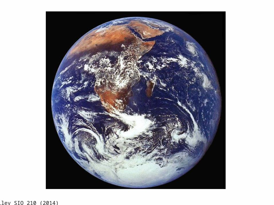
Atmospheric circulationL. Talley, SIO 210 Fall, 2014

• Vertical structure: troposphere, stratosphere, mesosphere, thermosphere

• Forcing: unequal distribution of solar radiation• Direct circulation

– Land and sea breeze– Monsoon– Equatorial: Walker circulation

• Mean large-scale wind and pressure structure– Hadley circulation– Jet Stream– Surface pressure– Surface wind stress

• Reading: Stewart Chapter 4• Other: DPO Chapter 5.8 (for wind patterns)

Talley SIO 210 (2014)


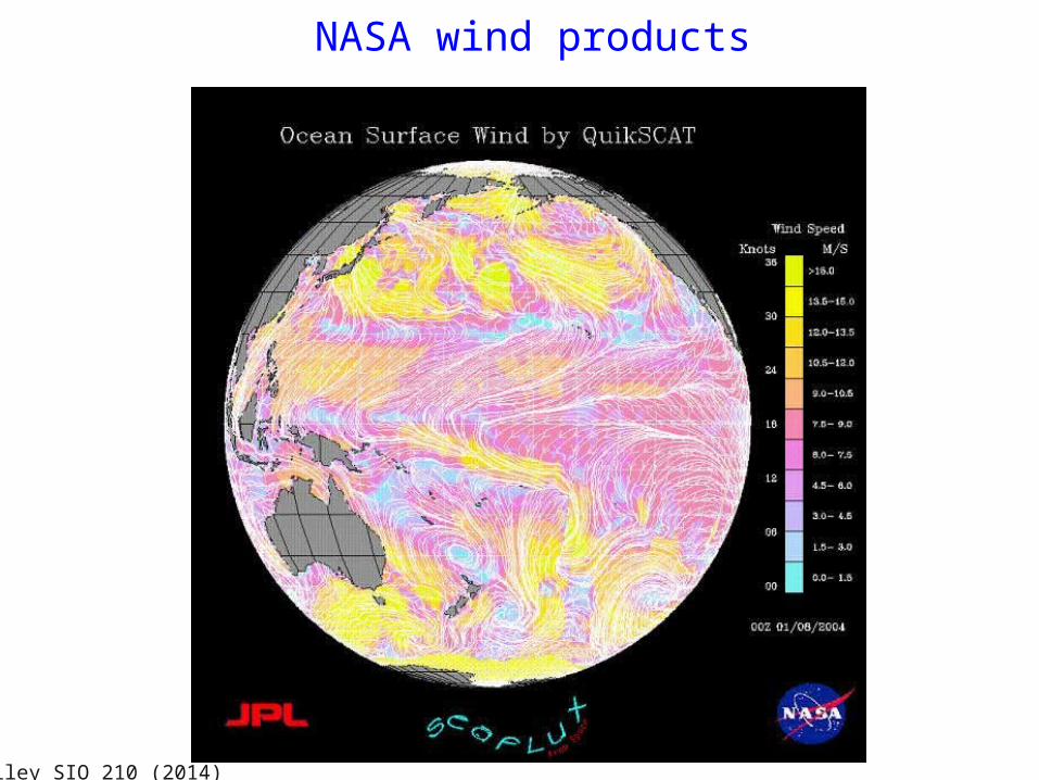
NASA wind products


Cloud cover


TALLEY Copyright © 2011 Elsevier Inc. All rights reserved

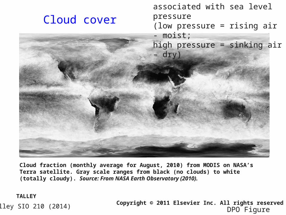
Cloud fraction (monthly average for August, 2010) from MODIS on NASA’s Terra satellite. Gray scale ranges from black (no clouds) to white (totally cloudy). Source: From NASA Earth Observatory (2010).

associated with sea level pressure (low pressure = rising air - moist; high pressure = sinking air – dry)

DPO Figure 5.8

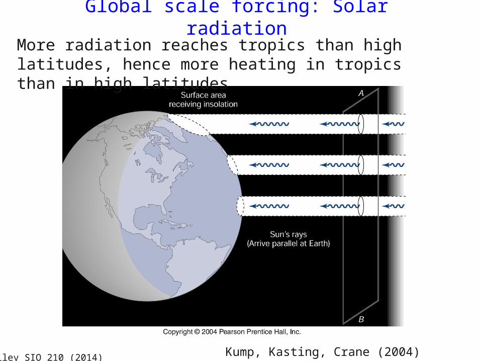
Global scale forcing: Solar radiationMore radiation reaches tropics than high latitudes, hence more heating in tropics than in high latitudes

Kump, Kasting, Crane (2004) textbookTalley SIO 210 (2014)

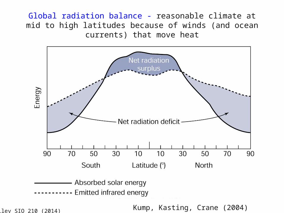
Global radiation balance - reasonable climate at mid to high latitudes because of winds (and ocean currents) that

move heat


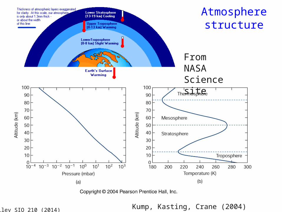
From NASA Science site

Atmosphere structure


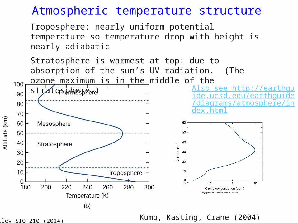
Atmospheric temperature structureTroposphere: nearly uniform potential temperature so temperature drop with height is nearly adiabatic

Stratosphere is warmest at top: due to absorption of the sun’s UV radiation. (The ozone maximum is in the middle of the stratosphere.)

Also see http://earthguide.ucsd.edu/earthguide/diagrams/atmosphere/index.html


http://earthguide.ucsd.edu/earthguide/diagrams/atmosphere/index.html



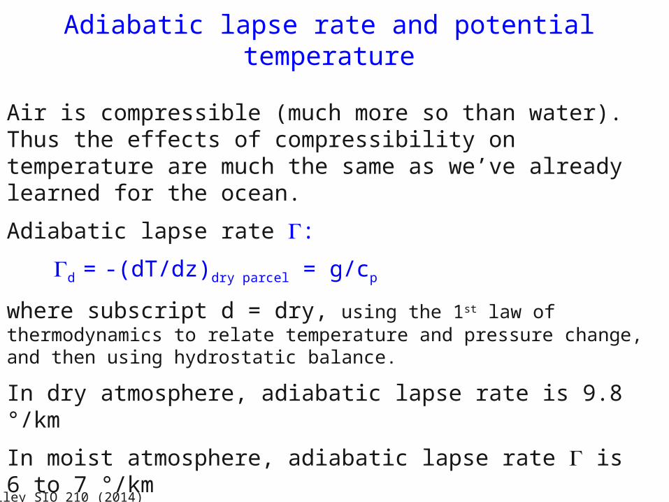
Adiabatic lapse rate and potential temperature

Air is compressible (much more so than water). Thus the effects of compressibility on temperature are much the same as we’ve already learned for the ocean.

Adiabatic lapse rate :

d = -(dT/dz)dry parcel = g/cp

where subscript d = dry, using the 1st law of thermodynamics to relate temperature and pressure change, and then using hydrostatic balance.

In dry atmosphere, adiabatic lapse rate is 9.8 °/km

In moist atmosphere, adiabatic lapse rate is 6 to 7 °/km

Potential temperature: reference level is the ground, taken as 1000 mbar.


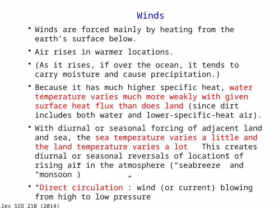
Winds• Winds are forced mainly by heating from the earth’s

surface below.

• Air rises in warmer locations.

• (As it rises, if over the ocean, it tends to carry moisture and cause precipitation.)

• Because it has much higher specific heat, water temperature varies much more weakly with given surface heat flux than does land (since dirt includes both water and lower-specific-heat air).

• With diurnal or seasonal forcing of adjacent land and sea, the sea temperature varies a little and the land temperature varies a lot. This creates diurnal or seasonal reversals of locations of rising air in the atmosphere (“seabreeze” and “monsoon”)

• “Direct circulation”: wind (or current) blowing from high to low pressure


Direct circulation

• “Direct circulation”: wind (or current) blowing from high to low pressure. Rotation effects are either negligible or relatively unimportant

• Examples presented here:

1. Diurnal winds (sea and land breeze, driven by land-sea temperature contrast)

2. Monsoonal winds (seasonal, driven by land-sea temperature contrast in the tropics where rotation is a minor factor)

3. Walker circulation (permanent, equatorial atmospheric circulation driven by zonal SST contrast)


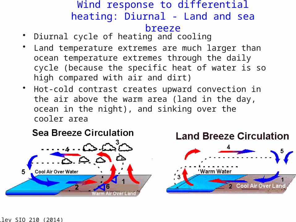
Wind response to differential heating: Diurnal - Land and sea breeze

• Diurnal cycle of heating and cooling• Land temperature extremes are much larger than ocean

temperature extremes through the daily cycle (because the specific heat of water is so high compared with air and dirt)

• Hot-cold contrast creates upward convection in the air above the warm area (land in the day, ocean in the night), and sinking over the cooler area


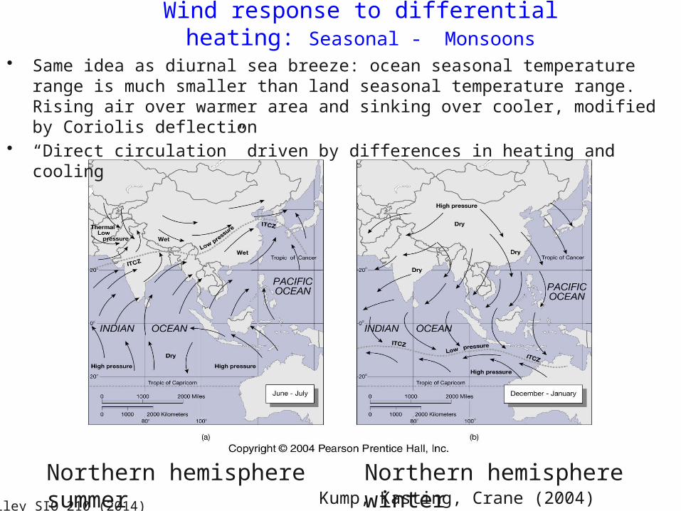
Wind response to differential heating: Seasonal - Monsoons

Northern hemisphere summer Northern hemisphere winter

• Same idea as diurnal sea breeze: ocean seasonal temperature range is much smaller than land seasonal temperature range. Rising air over warmer area and sinking over cooler, modified by Coriolis deflection

• “Direct circulation” driven by differences in heating and cooling


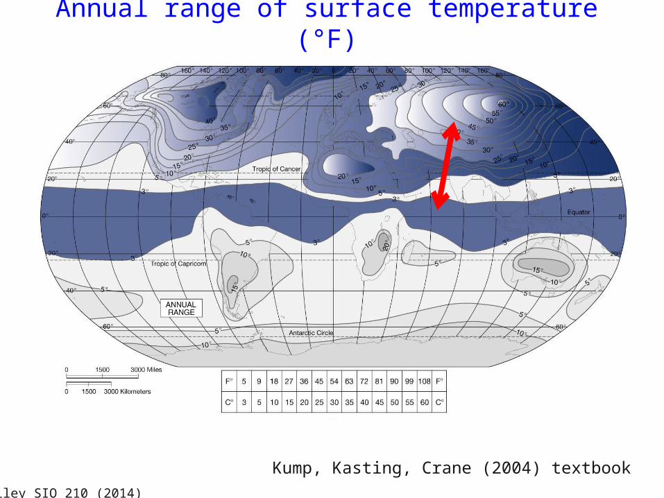
Annual range of surface temperature (°F)



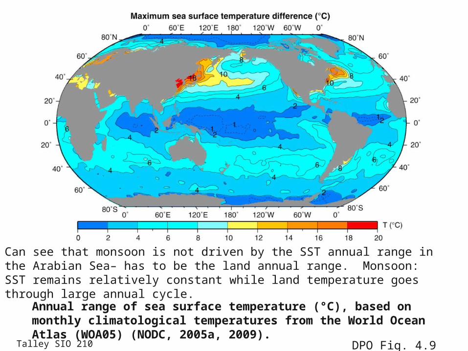
Annual range of sea surface temperature (°C), based on monthly climatological temperatures from the World Ocean Atlas (WOA05) (NODC, 2005a, 2009).

Can see that monsoon is not driven by the SST annual range in the Arabian Sea– has to be the land annual range. Monsoon: SST remains relatively constant while land temperature goes through large annual cycle.

DPO Fig. 4.9

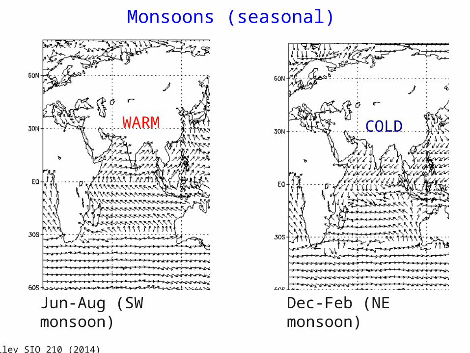
Monsoons (seasonal)

Dec-Feb (NE monsoon)Jun-Aug (SW monsoon)

WARM COLD


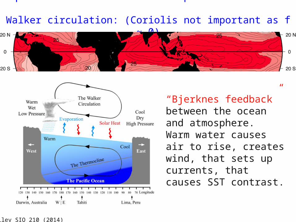
Equatorial winds: Direct atmospheric circulation Walker circulation: (Coriolis not important as f ~ 0)

“Bjerknes feedback” between the ocean and atmosphere.Warm water causes air to rise, creates wind, that sets up currents, that causes SST contrast.


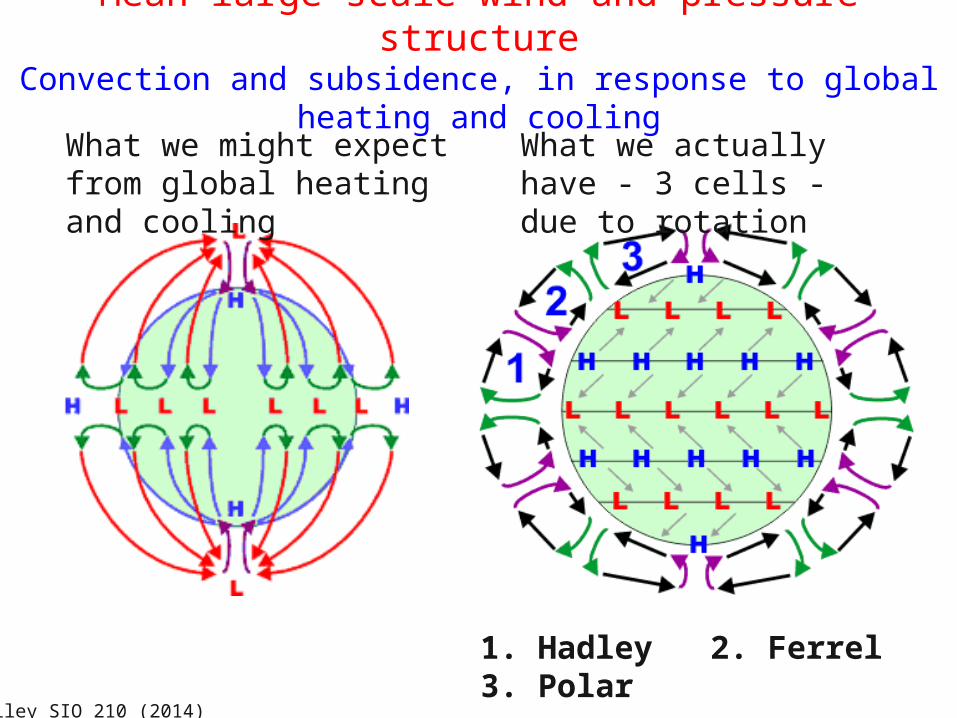
Mean large-scale wind and pressure structureConvection and subsidence, in response to global heating

and cooling

What we actually have - 3 cells - due to rotation

What we might expect from global heating and cooling

1. Hadley 2. Ferrel 3. Polar


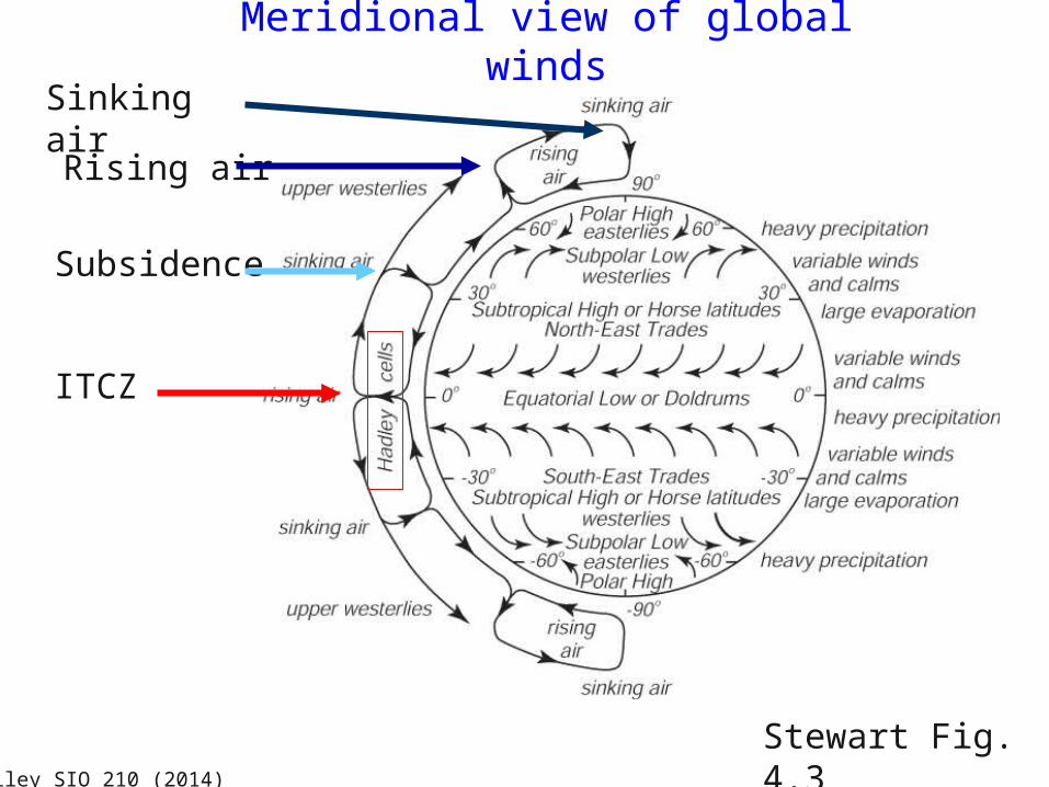
Meridional view of global winds

ITCZ

Stewart Fig. 4.3

Subsidence

Rising air

Sinking air


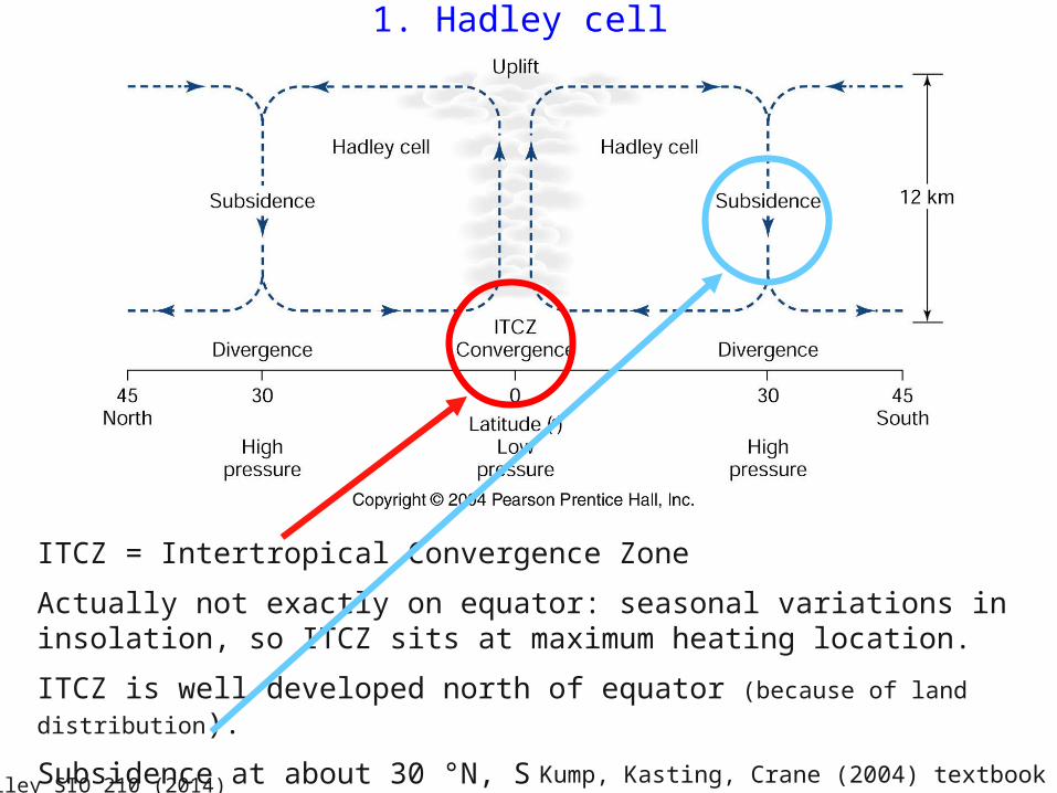
ITCZ = Intertropical Convergence Zone

Actually not exactly on equator: seasonal variations in insolation, so ITCZ sits at maximum heating location.

ITCZ is well developed north of equator (because of land distribution).

Subsidence at about 30 °N, S

1. Hadley cell


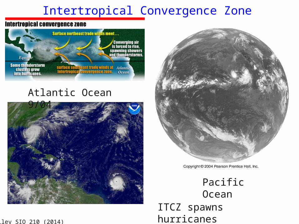
Atlantic Ocean 9/04

Pacific Ocean

Intertropical Convergence Zone

ITCZ spawns hurricanesTalley SIO 210 (2014)

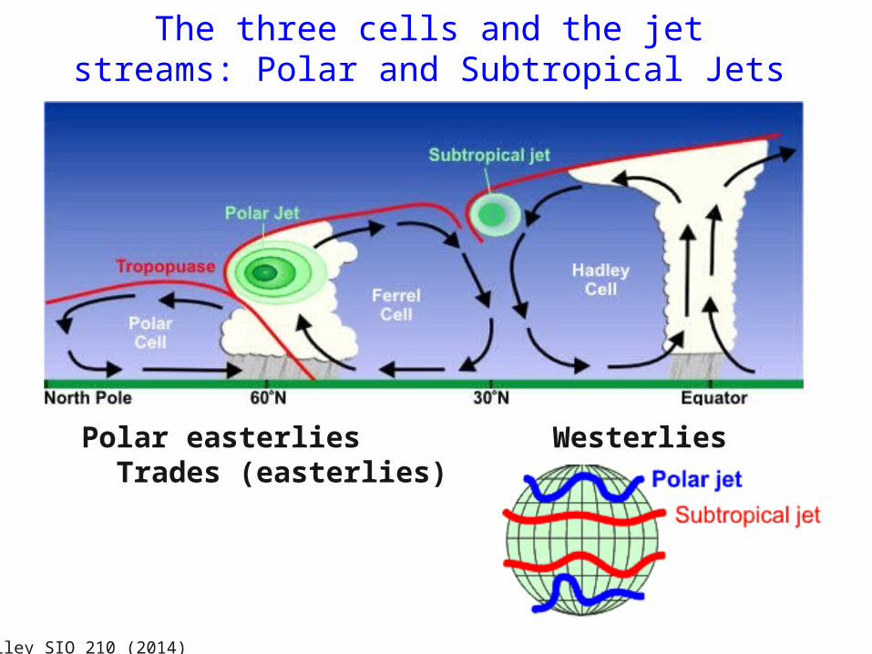
The three cells and the jet streams: Polar and Subtropical Jets

Polar easterlies Westerlies Trades (easterlies)


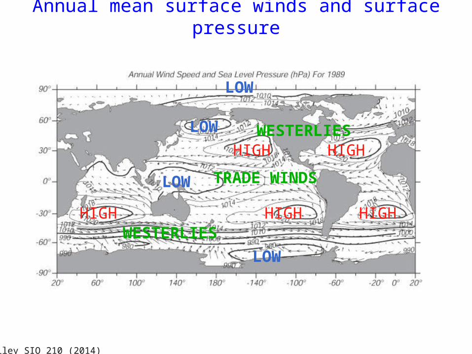
Annual mean surface winds and surface pressure

HIGH HIGH

HIGH HIGHHIGH

LOW

LOW

LOW

LOW

TRADE WINDS

WESTERLIES

WESTERLIES


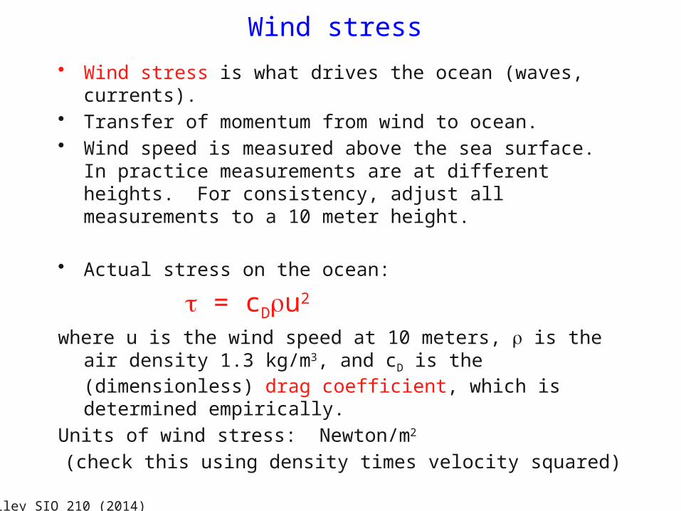
Wind stress

• Wind stress is what drives the ocean (waves, currents).• Transfer of momentum from wind to ocean.• Wind speed is measured above the sea surface. In

practice measurements are at different heights. For consistency, adjust all measurements to a 10 meter height.

• Actual stress on the ocean:

= cDu2 where u is the wind speed at 10 meters, is the air density

1.3 kg/m3, and cD is the (dimensionless) drag coefficient, which is determined empirically.

Units of wind stress: Newton/m2

(check this using density times velocity squared)


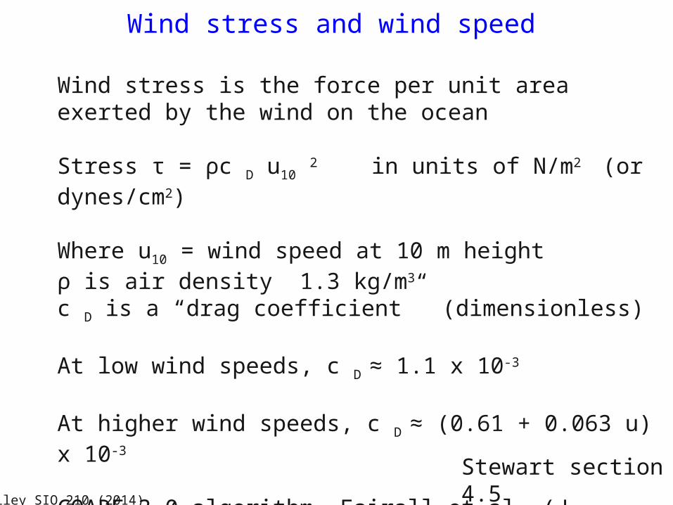
Wind stress and wind speed

Wind stress is the force per unit area exerted by the wind on the ocean

Stress τ = ρc D u10 2 in units of N/m2 (or dynes/cm2)

Where u10 = wind speed at 10 m heightρ is air density 1.3 kg/m3

c D is a “drag coefficient” (dimensionless)

At low wind speeds, c D ≈ 1.1 x 10-3

At higher wind speeds, c D ≈ (0.61 + 0.063 u) x 10-3

COARE 3.0 algorithm Fairall et al. (J. Climate 2003)Stewart section 4.5


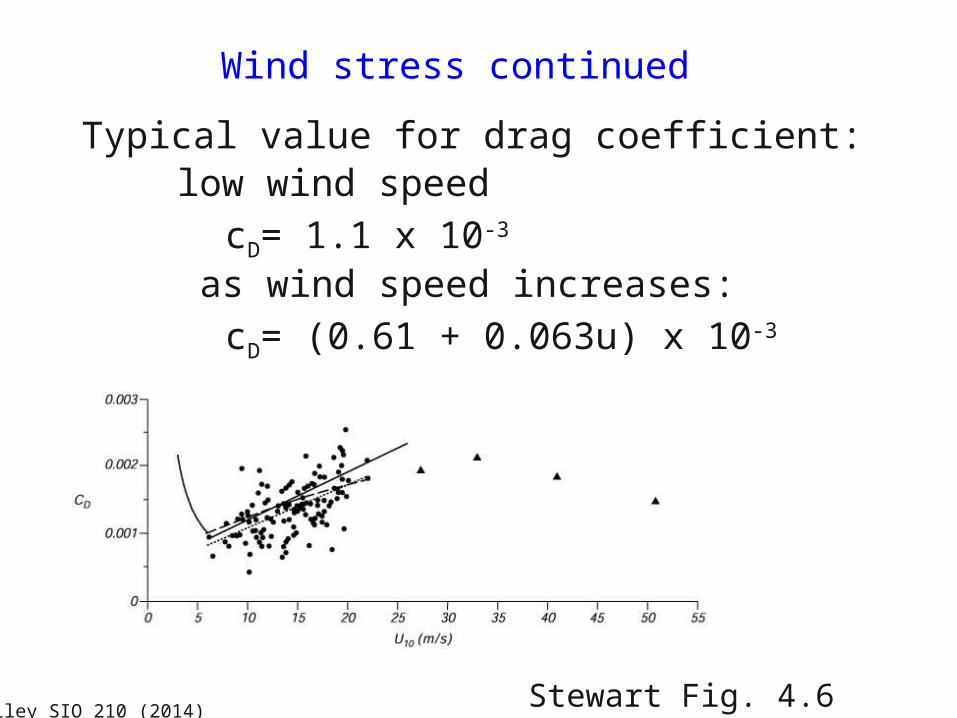
Wind stress continued

Typical value for drag coefficient: low wind speed

cD= 1.1 x 10-3

as wind speed increases:

cD= (0.61 + 0.063u) x 10-3

Stewart Fig. 4.6Talley SIO 210 (2014)

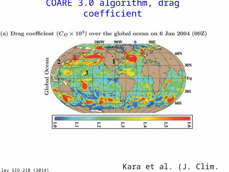
COARE 3.0 algorithm, drag coefficient

Kara et al. (J. Clim. 2007)Talley SIO 210 (2014)

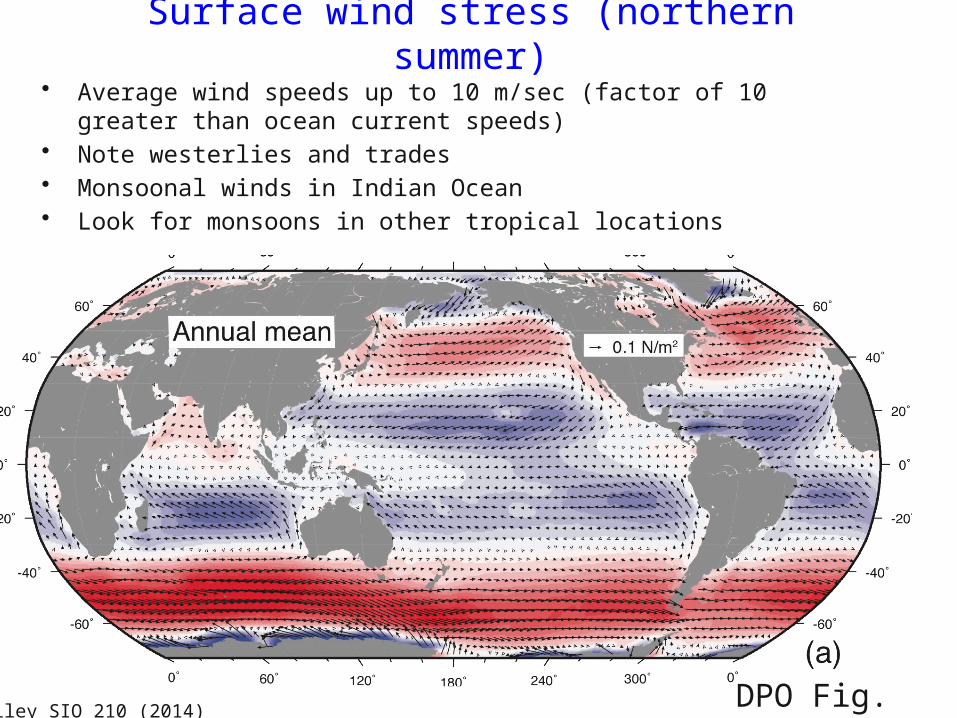
DPO Fig. 5.16a

Surface wind stress (northern summer)• Average wind speeds up to 10 m/sec (factor of 10 greater than

ocean current speeds)• Note westerlies and trades• Monsoonal winds in Indian Ocean• Look for monsoons in other tropical locations


Documents

Atmospheric circulation L. Talley, SIO 210 Fall, 2014 Vertical structure: troposphere, stratosphere, mesosphere, thermosphere Forcing: unequal distribution