Embed Size (px)
Citation preview
ENVIRONMENTALDOCUMENTATION No. 116
Air
Atmospheric Depositionof Nitrogen to theSwiss Seeland Region
Author Werner EugsterUniversity of Bern, Geographical Institute
Project Members Heinz WannerSilvan PeregoAlex LeuenbergerMatthias LiechtiMarkus ReinhardtPeter GeissbuhlerMarion GempelerJurg SchenkUniversity of Bern, Geographical Institute
Language editing Christopher E. Sidle
Project management Paul FilligerSwiss Agency for the Environment, Forests and Landscape, Bern
Distributed by Swiss Agency for the Environment, Forests and LandscapeDocumentationCH – 3003 Bern
Fax +41 (0)31 324 02 16E-mail: [email protected]: http://www.admin.ch/buwal/publikat/d/
Order number UM-116-E
Price Sfr. 15.—
c⃝ SAEFL 1999 11.99 600 10V10176
Contents
Abstracts 5
Preface 7
Summaries 9
1 Introduction 171.1 Purpose of the Study . . . . . . . . . . . . . . . . . . . . . . . . . . . . . 171.2 Scientific Work Carried out . . . . . . . . . . . . . . . . . . . . . . . . . 18
2 The Role of Nitrogen Deposition in the Nitrogen Cycle 21
3 The Study Area: the Swiss Seeland 253.1 Overview . . . . . . . . . . . . . . . . . . . . . . . . . . . . . . . . . . . 253.2 Landscape Evolution and Development . . . . . . . . . . . . . . . . . . . 293.3 Land Use in 1994 . . . . . . . . . . . . . . . . . . . . . . . . . . . . . . . 313.4 Climate . . . . . . . . . . . . . . . . . . . . . . . . . . . . . . . . . . . . 32
4 Modeling Approach 384.1 Overview . . . . . . . . . . . . . . . . . . . . . . . . . . . . . . . . . . . 384.2 Model Design . . . . . . . . . . . . . . . . . . . . . . . . . . . . . . . . . 384.3 Model Domain . . . . . . . . . . . . . . . . . . . . . . . . . . . . . . . . 394.4 Boundary Conditions . . . . . . . . . . . . . . . . . . . . . . . . . . . . . 404.5 Deposition Module . . . . . . . . . . . . . . . . . . . . . . . . . . . . . . 40
4.5.1 Aerodynamic Resistance Ra . . . . . . . . . . . . . . . . . . . . . 414.5.2 Laminar Boundary Layer Resistance Rb . . . . . . . . . . . . . . . 414.5.3 Canopy Resistance Rc . . . . . . . . . . . . . . . . . . . . . . . . 44
4.6 Strengths and Weaknesses of the Model . . . . . . . . . . . . . . . . . . 454.7 Concluding Remarks . . . . . . . . . . . . . . . . . . . . . . . . . . . . . 46
5 Selection of Representative Days and Model Inputs 485.1 Classification of Turbulent Transport Conditions . . . . . . . . . . . . . . 485.2 Selection of Representative Days for Modeling . . . . . . . . . . . . . . . 515.3 Emission Inventory for Ammonia . . . . . . . . . . . . . . . . . . . . . . 52
5.3.1 Comparison with the Emission Factor Method . . . . . . . . . . . 555.4 Emission Inventories for Other Trace Gases . . . . . . . . . . . . . . . . . 575.5 Meteorological Inputs . . . . . . . . . . . . . . . . . . . . . . . . . . . . 57
6 Dry Deposition of Nitrogen 596.1 Introduction . . . . . . . . . . . . . . . . . . . . . . . . . . . . . . . . . . 596.2 Seasonal and Regional Variation . . . . . . . . . . . . . . . . . . . . . . . 59
3

4 CONTENTS
6.2.1 Total Nitrogen Deposition . . . . . . . . . . . . . . . . . . . . . . 606.2.2 Deposition of Oxidized Nitrogen . . . . . . . . . . . . . . . . . . 626.2.3 Deposition of Reduced Nitrogen . . . . . . . . . . . . . . . . . . . 656.2.4 Ratio Between Local Emissions and Local Deposition Totals . . . 69
6.3 Regional Variation of Individual Turbulent Transport Classes . . . . . . . 69
7 Wet Deposition of Nitrogen 757.1 Introduction . . . . . . . . . . . . . . . . . . . . . . . . . . . . . . . . . . 757.2 Working Hypotheses . . . . . . . . . . . . . . . . . . . . . . . . . . . . . 757.3 The Schenk-type Wet-only Samplers . . . . . . . . . . . . . . . . . . . . 767.4 Methods . . . . . . . . . . . . . . . . . . . . . . . . . . . . . . . . . . . . 777.5 Sites . . . . . . . . . . . . . . . . . . . . . . . . . . . . . . . . . . . . . . 777.6 Scaling up to Annual Wet Deposition Estimates . . . . . . . . . . . . . . 78
7.6.1 First Approach . . . . . . . . . . . . . . . . . . . . . . . . . . . . 797.6.2 Second Approach . . . . . . . . . . . . . . . . . . . . . . . . . . . 807.6.3 Comparison Between the two Approaches . . . . . . . . . . . . . 80
7.7 Results . . . . . . . . . . . . . . . . . . . . . . . . . . . . . . . . . . . . . 80
8 Dry Deposition of Aerosol Particles 858.1 Introduction . . . . . . . . . . . . . . . . . . . . . . . . . . . . . . . . . . 858.2 Data used . . . . . . . . . . . . . . . . . . . . . . . . . . . . . . . . . . . 858.3 Height profile of dry particulate deposition: sedimentation . . . . . . . . 868.4 Impaction and diffusive deposition of small aerosol particles . . . . . . . 87
8.4.1 Nitrogen content estimation . . . . . . . . . . . . . . . . . . . . . 878.4.2 Dry deposition velocity estimation . . . . . . . . . . . . . . . . . 898.4.3 Deposition estimation . . . . . . . . . . . . . . . . . . . . . . . . 89
8.5 Total aerosol deposition . . . . . . . . . . . . . . . . . . . . . . . . . . . 90
9 Comparison with Swiss Study and Open Questions 939.1 Differences between this study and Rihm (1996) . . . . . . . . . . . . . 939.2 Open Questions . . . . . . . . . . . . . . . . . . . . . . . . . . . . . . . . 94
9.2.1 Ammonia Deposition to Open Water . . . . . . . . . . . . . . . . 949.2.2 Occult Deposition . . . . . . . . . . . . . . . . . . . . . . . . . . . 959.2.3 Conversion of Ammonia to Ammonium . . . . . . . . . . . . . . . 959.2.4 The Role of Oxidation of NOx to HNO3 . . . . . . . . . . . . . . . 95
10 Discussion and Conclusions 9610.1 Rural Plains of the Seeland . . . . . . . . . . . . . . . . . . . . . . . . . 9810.2 The Lower Jura South Slope . . . . . . . . . . . . . . . . . . . . . . . . . 9910.3 Lakes and Other Water Bodies . . . . . . . . . . . . . . . . . . . . . . . . 10010.4 The Urban Area of Bern . . . . . . . . . . . . . . . . . . . . . . . . . . . 10010.5 Forested Hills in the Seeland . . . . . . . . . . . . . . . . . . . . . . . . . 10110.6 Annual Average of the Entire Model Domain . . . . . . . . . . . . . . . . 10210.7 Conclusions . . . . . . . . . . . . . . . . . . . . . . . . . . . . . . . . . . 102
Index 107
A Color Plates 109
Abstracts
English
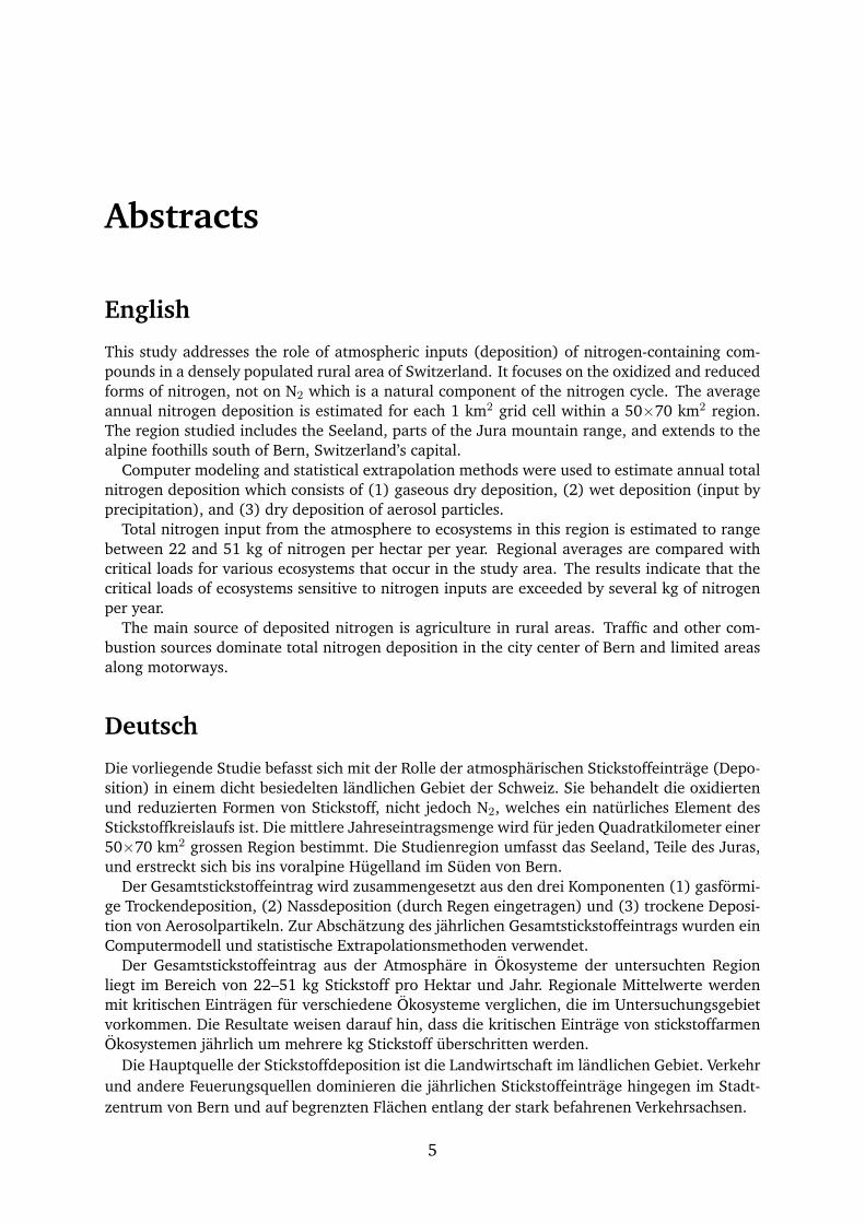
This study addresses the role of atmospheric inputs (deposition) of nitrogen-containing com-pounds in a densely populated rural area of Switzerland. It focuses on the oxidized and reducedforms of nitrogen, not on N2 which is a natural component of the nitrogen cycle. The averageannual nitrogen deposition is estimated for each 1 km2 grid cell within a 50×70 km2 region.The region studied includes the Seeland, parts of the Jura mountain range, and extends to thealpine foothills south of Bern, Switzerland’s capital.
Computer modeling and statistical extrapolation methods were used to estimate annual totalnitrogen deposition which consists of (1) gaseous dry deposition, (2) wet deposition (input byprecipitation), and (3) dry deposition of aerosol particles.
Total nitrogen input from the atmosphere to ecosystems in this region is estimated to rangebetween 22 and 51 kg of nitrogen per hectar per year. Regional averages are compared withcritical loads for various ecosystems that occur in the study area. The results indicate that thecritical loads of ecosystems sensitive to nitrogen inputs are exceeded by several kg of nitrogenper year.
The main source of deposited nitrogen is agriculture in rural areas. Traffic and other com-bustion sources dominate total nitrogen deposition in the city center of Bern and limited areasalong motorways.
Deutsch
Die vorliegende Studie befasst sich mit der Rolle der atmospharischen Stickstoffeintrage (Depo-sition) in einem dicht besiedelten landlichen Gebiet der Schweiz. Sie behandelt die oxidiertenund reduzierten Formen von Stickstoff, nicht jedoch N2, welches ein naturliches Element desStickstoffkreislaufs ist. Die mittlere Jahreseintragsmenge wird fur jeden Quadratkilometer einer50×70 km2 grossen Region bestimmt. Die Studienregion umfasst das Seeland, Teile des Juras,und erstreckt sich bis ins voralpine Hugelland im Suden von Bern.
Der Gesamtstickstoffeintrag wird zusammengesetzt aus den drei Komponenten (1) gasformi-ge Trockendeposition, (2) Nassdeposition (durch Regen eingetragen) und (3) trockene Deposi-tion von Aerosolpartikeln. Zur Abschatzung des jahrlichen Gesamtstickstoffeintrags wurden einComputermodell und statistische Extrapolationsmethoden verwendet.
Der Gesamtstickstoffeintrag aus der Atmosphare in Okosysteme der untersuchten Regionliegt im Bereich von 22–51 kg Stickstoff pro Hektar und Jahr. Regionale Mittelwerte werdenmit kritischen Eintragen fur verschiedene Okosysteme verglichen, die im Untersuchungsgebietvorkommen. Die Resultate weisen darauf hin, dass die kritischen Eintrage von stickstoffarmenOkosystemen jahrlich um mehrere kg Stickstoff uberschritten werden.
Die Hauptquelle der Stickstoffdeposition ist die Landwirtschaft im landlichen Gebiet. Verkehrund andere Feuerungsquellen dominieren die jahrlichen Stickstoffeintrage hingegen im Stadt-zentrum von Bern und auf begrenzten Flachen entlang der stark befahrenen Verkehrsachsen.
5
6 ABSTRACT
Francais
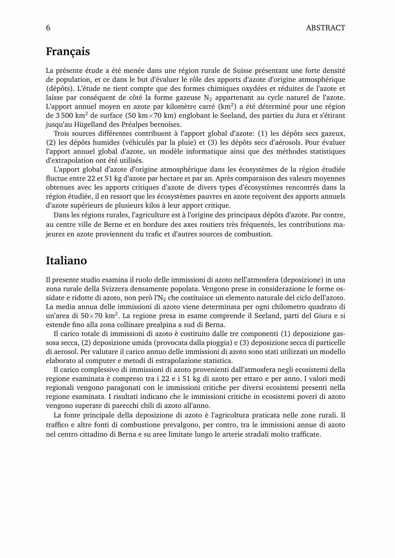
La presente etude a ete menee dans une region rurale de Suisse presentant une forte densitede population, et ce dans le but d’evaluer le role des apports d’azote d’origine atmospherique(depots). L’etude ne tient compte que des formes chimiques oxydees et reduites de l’azote etlaisse par consequent de cote la forme gazeuse N2 appartenant au cycle naturel de l’azote.L’apport annuel moyen en azote par kilometre carre (km2) a ete determine pour une regionde 3 500 km2 de surface (50 km×70 km) englobant le Seeland, des parties du Jura et s’etirantjusqu’au Hugelland des Prealpes bernoises.
Trois sources differentes contribuent a l’apport global d’azote: (1) les depots secs gazeux,(2) les depots humides (vehicules par la pluie) et (3) les depots secs d’aerosols. Pour evaluerl’apport annuel global d’azote, un modele informatique ainsi que des methodes statistiquesd’extrapolation ont ete utilises.
L’apport global d’azote d’origine atmospherique dans les ecosystemes de la region etudieefluctue entre 22 et 51 kg d’azote par hectare et par an. Apres comparaison des valeurs moyennesobtenues avec les apports critiques d’azote de divers types d’ecosystemes rencontres dans laregion etudiee, il en ressort que les ecosystemes pauvres en azote recoivent des apports annuelsd’azote superieurs de plusieurs kilos a leur apport critique.
Dans les regions rurales, l’agriculture est a l’origine des principaux depots d’azote. Par contre,au centre ville de Berne et en bordure des axes routiers tres frequentes, les contributions ma-jeures en azote proviennent du trafic et d’autres sources de combustion.
Italiano
Il presente studio esamina il ruolo delle immissioni di azoto nell’atmosfera (deposizione) in unazona rurale della Svizzera densamente popolata. Vengono prese in considerazione le forme os-sidate e ridotte di azoto, non pero l’N2 che costituisce un elemento naturale del ciclo dell’azoto.La media annua delle immissioni di azoto viene determinata per ogni chilometro quadrato diun’area di 50×70 km2. La regione presa in esame comprende il Seeland, parti del Giura e siestende fino alla zona collinare prealpina a sud di Berna.
Il carico totale di immissioni di azoto e costituito dalle tre componenti (1) deposizione gas-sosa secca, (2) deposizione umida (provocata dalla pioggia) e (3) deposizione secca di particelledi aerosol. Per valutare il carico annuo delle immissioni di azoto sono stati utilizzati un modelloelaborato al computer e metodi di estrapolazione statistica.
Il carico complessivo di immissioni di azoto provenienti dall’atmosfera negli ecosistemi dellaregione esaminata e compreso tra i 22 e i 51 kg di azoto per ettaro e per anno. I valori mediregionali vengono paragonati con le immissioni critiche per diversi ecosistemi presenti nellaregione esaminata. I risultati indicano che le immissioni critiche in ecosistemi poveri di azotovengono superate di parecchi chili di azoto all’anno.
La fonte principale della deposizione di azoto e l’agricoltura praticata nelle zone rurali. Iltraffico e altre fonti di combustione prevalgono, per contro, tra le immissioni annue di azotonel centro cittadino di Berna e su aree limitate lungo le arterie stradali molto trafficate.
Foreword
Nitrogen in its various chemical forms plays a major role in a great number of environ-mental issues. In excess amounts, it contributes to acidification and eutrophication ofthe soil and surface waters and leads to a decrease in ecosystem vitality and biodiver-sity. In the atmosphere, nitrogen compounds play an important role in the formationof ozone, oxidants and aerosols, potentially posing a threat to human health and plantgrowth.
In the framework of the UN/ECE Convention on Long-range Transboundary Air Pol-lution, critical levels and loads have been defined and an extensive mapping activity iscarried out in Europe. The main task of these activities is the mapping of the sensitiv-ity of receptors to air pollution, the current levels of ozone, the current deposition ofacidifying and eutrophying compounds, and the resulting exceedances of critical levelsand critical loads. In addition to the national and European scale mapping activities,local case studies are necessary. They give the possibility to compare the large scale re-sults with results from local studies which are based on different models with differentparameterisations of the processes.
To understand the nitrogen cycle in the atmosphere, emission, transport and depo-sition of oxidised as well as reduced nitrogen compounds have to be considered. Asthis study shows, 50–80% of total nitrogen deposition is reduced nitrogen which is lostto the atmosphere from agricultural sources. Therefore, ammonia emissions are veryimportant in studying nitrogen deposition to semi-natural ecosystems.
The modelling of the complete nitrogen cycle in the atmosphere is a rather chal-lenging task and many questions are still open. This study shall stimulate the scientificdiscussion on this subject and contribute to the mapping activities realised in the frame-work of the UN/ECE Convention.
Gerhard Leutert
Head of the Air Pollution Control Division
7

8 FOREWORD
Summaries
English
Nitrogen is essential for plant growthand thus also for food production. Be-cause the chemical form of nitrogenmost abundant in the atmosphere (N2)is not directly accessible to plants, largeamounts of fertilizers, containing oxi-dized and reduced forms of nitrogen,are used world-wide for food produc-tion. Various other human activities alsorelease significant amounts of oxidized(NOx) and reduced nitrogen compounds(NHx) into the environment, includingthe atmosphere. Because these com-pounds are directly available to plants,they contribute to the eutrophication ofecosystems.
Ecosystems are generally adapted tothe much lower nitrogen inputs theyreceive from nitrogen-fixing soil micro-organisms (which are capable of con-verting atmospheric N2 into oxidized andreduced chemical forms). Therefore, itis expected that additional inputs of oxi-dized and reduced nitrogen originatingfrom human activities may exhibit animporant impact on natural and semi-natural ecosystems. Malnutrition, lossof species diversity, and shifts in speciescomposition of ecosystems are some ofthe most apparent effects that nitrogencritical loads exceedances are expectedto impose on plant communities. Ani-mals and animal communities that feedon specific plants, or which would be af-fected by disturbance of the complex nu-trition web would then also experiencesignificant changes in their environment,and may eventually disappear.
This study addresses the role of atmo-spheric inputs (deposition) of nitrogen-containing compounds in a densely pop-ulated rural area of Switzerland that alsoincludes minor cities and towns. It fo-cuses on the oxidized and reduced formsof nitrogen, not on N2 which is a natu-ral component of the nitrogen cycle. Theaverage annual nitrogen deposition is es-timated for each 1 km2 grid cell withina 50×70 km2 region. The region stud-ied includes the Seeland, parts of theJura mountain range, and extends to thealpine foothills south of Bern, Switzer-land’s capital.
Total nitrogen deposition consists of(1) gaseous dry deposition, (2) wet de-position (input by precipitation), and(3) dry deposition of aerosol particles.Numerical computer modeling was em-ployed to estimate deposition of gaseouscompounds (e.g. ammonia NH3, nitricoxide NO, nitrogen dioxide NO2), whilewet deposition and aerosol depositionwere estimated via the extrapolation offield data over the study area.
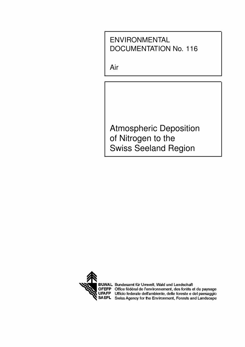
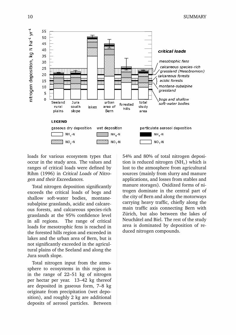
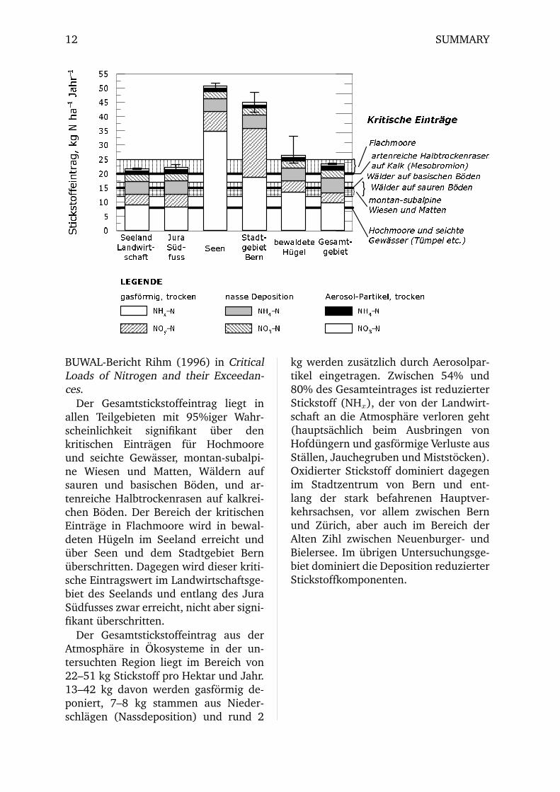
The annual estimates for each grid cellof the study area were then groupedto obtain regional averages (figure nextpage) for characteristic land-use typesand localities within the study area. Thebars show the annual average nitrogendeposition per hectar, and the error barsindicate the 95% confidence interval forthe annual loads. The shading of thebars shows the fractions of reduced andoxidized nitrogen, respectively, for eachof the three deposition components thatwere included in this analysis.
The horizontal lines in the backgroundof this figure show the nutrient critical
9
10 SUMMARY
��
��������������������
QLWURJH
Q�GHS
RVLWLR
Q��NJ
�1�KD
���\U
��
-XUDVRXWKVORSH
ODNHV6HHODQGUXUDOSODLQV
XUEDQDUHD�RI%HUQ
IRUHVWHGKLOOV
WRWDOVWXG\DUHD
}
}}
PHVRWURSKLF�IHQV
DFLGLF�IRUHVWVPRQWDQH�VXEDOSLQHJUDVVODQG
ERJV�DQG�VKDOORZVRIW�ZDWHU�ERGLHV
FDOFDUHRXV�IRUHVWV
FDOFDUHRXV�VSHFLHV�ULFKJUDVVODQG��0HVREURPLRQ�
FULWLFDO�ORDGV
1+[�112\�1
1+��112��1
1+��112��1
JDVHRXV�GU\�GHSRVLWLRQ ZHW�GHSRVLWLRQ SDUWLFXODWH�DHURVRO�GHSRVLWLRQ/(*(1'
loads for various ecosystem types thatoccur in the study area. The values andranges of critical loads were defined byRihm (1996) in Critical Loads of Nitro-gen and their Exceedances.
Total nitrogen deposition significantlyexceeds the critical loads of bogs andshallow soft-water bodies, montane-subalpine grasslands, acidic and calcare-ous forests, and calcareous species-richgrasslands at the 95% confidence levelin all regions. The range of criticalloads for mesotrophic fens is reached inthe forested hills region and exceeded inlakes and the urban area of Bern, but isnot significantly exceeded in the agricul-tural plains of the Seeland and along theJura south slope.
Total nitrogen input from the atmo-sphere to ecosystems in this region isin the range of 22–51 kg of nitrogenper hectar per year. 13–42 kg thereofare deposited in gaseous form, 7–8 kgoriginate from precipitation (wet depo-sition), and roughly 2 kg are additionaldeposits of aerosol particles. Between
54% and 80% of total nitrogen deposi-tion is reduced nitrogen (NHx) which islost to the atmosphere from agriculturalsources (mainly from slurry and manureapplications, and losses from stables andmanure storages). Oxidized forms of ni-trogen dominate in the central part ofthe city of Bern and along the motorwayscarrying heavy traffic, chiefly along themain traffic axis connecting Bern withZurich, but also between the lakes ofNeuchatel and Biel. The rest of the studyarea is dominated by deposition of re-duced nitrogen compounds.
SUMMARY 11
Deutsch
Stickstoff ist notwendig fur das Pflan-zenwachstum und somit auch fur dieErnahrung der Weltbevolkerung. Weildie chemische Form von Stickstoff, diein der Atmosphare am haufigsten ist(N2), nicht direkt pflanzenverfugbar ist,werden in der Landwirtschaft weltweitgrosse Mengen von Dungern verwendet,welche oxidierte und reduzierte Stick-stoffformen beinhalten. Bei verschiede-nen anderen menschlichen Tatigkeitenwerden ebenfalls grosse Mengen oxidier-ter (NOx) und reduzierter Stickstoffver-bindungen (NHx) an die Umwelt abge-geben, auch an die Atmosphare. Weildiese Verbindungen direkt zur Pflanze-nernahrung beitragen, fuhren sie auchzu einer Eutrophierung von Okosyste-men.
Okosysteme sind grundsatzlich an dieviel kleineren Stickstoffeintrage, welchesie von Stickstoff fixierenden Bodenmi-kroorganismen erhalten, angepasst (die-se besitzen die Fahigkeit, atmosphari-sches N2 in oxidierte und reduzier-te Stickstoffformen umzuwandeln). Des-halb wird angenommen, dass zusatzlicheEintrage von oxidiertem und reduzier-tem Stickstoff aus menschlichen Quelleneinen bedeutenden Einfluss auf naturli-che und naturnahe Okosysteme haben.Mangelerscheinungen, Verlust an Biodi-versitat und Veranderungen in der Ar-tenzusammensetzung von Okosystemensind einige der wichtigsten Effekte, diedurch das Uberschreiten der kritischenStickstoffeintragsmengen (critical loads)verursacht werden konnen. Tiere undTiergemeinschaften, die sich von speziel-len Pflanzenarten ernahren oder die an-derweitig durch die komplexe Nahrungs-kette beeinflusst werden, konnten erheb-lich in ihrer Umgebung beeintrachtigtwerden und eventuell aussterben.
Die vorliegende Studie befasst sich mitder Rolle der atmospharischen Stickstof-
feintrage (Deposition) in einem dicht be-siedelten landlichen Gebiet der Schweiz,welches auch kleinere Stadte und grosse-re Dorfer umfasst. Sie behandelt dieoxidierten und reduzierten Formen vonStickstoff, nicht jedoch N2, welches einnaturliches Element des Stickstoffkreis-laufs ist. Die mittlere Jahreseintrags-menge wird fur jeden Quadratkilome-ter einer 50×70 km2 grossen Region be-stimmt. Die Studienregion umfasst dasSeeland, Teile des Juras, und erstrecktsich bis ins voralpine Hugelland imSuden von Bern.
Der Gesamtstickstoffeintrag wird zu-sammengesetzt aus den drei Komponen-ten (1) gasformige Trockendeposition,(2) Nassdeposition (durch Regen ein-getragen) und (3) trockene Depositionvon Aerosolpartikeln. Ein Computermo-dell wurde verwendet zur Bestimmungder Trockendeposition gasformiger Sub-stanzen (z.B. Ammoniak NH3, Stick-oxid NO, Stickstoffdioxid NO2), wahrenddie Nassdeposition und Aerosoldeposi-tion anhand von Messdaten geschatztwurde, die fur das Untersuchungsgebietraumlich extrapoliert wurden.
Die Jahresfrachten jedes Quadratkilo-meters des Untersuchungsgebiets wur-den zu regionalen Mitteln ausgewahl-ter Teilgebiete zusammengefasst (Abbil-dung nachste Seite). Die Saulen zeigendie mittleren Jahressummen der Stick-stoffdeposition pro Hektar. Die verti-kalen Fehlerbalken definieren das 95%Konfidenzintervall der jahrlichen Ein-trage. Die Schattierung der Saulen zeigtdie jeweiligen Anteile von reduziertenund oxidierten Stickstoffformen der dreiin dieser Untersuchung berucksichtigtenDepositionsarten.
Die horizontalen Linien im Hinter-grund dieser Abbildung zeigen die kri-tischen Stickstoffeintrage ausgewahlterOkosystemtypen, die im Untersuchungs-gebiet vorkommen. Die kritischen Wer-te und Bereiche wurden festgelegt im
12 SUMMARY
��
��������������������
6WLFN
VWRIIH
LQWUDJ
��NJ�1
�KD���-D
KU��
-XUD6�G�IXVV
6HHQ6HHODQG/DQGZLUW�VFKDIW
6WDGW�JHELHW%HUQ
EHZDOGHWH+�JHO
*HVDPW�JHELHW
}
}}
)ODFKPRRUH
:lOGHU�DXI�VDXUHQ�%|GHQPRQWDQ�VXEDOSLQH:LHVHQ�XQG�0DWWHQ
+RFKPRRUH�XQG�VHLFKWH*HZlVVHU��7�PSHO�HWF��
:lOGHU�DXI�EDVLVFKHQ�%|GHQ
DUWHQUHLFKH�+DOEWURFNHQUDVHQDXI�.DON��0HVREURPLRQ�
.ULWLVFKH�(LQWUlJH
1+[�112\�1
1+��112��1
1+��112��1
JDVI|UPLJ��WURFNHQ QDVVH�'HSRVLWLRQ $HURVRO�3DUWLNHO��WURFNHQ/(*(1'(
BUWAL-Bericht Rihm (1996) in CriticalLoads of Nitrogen and their Exceedan-ces.
Der Gesamtstickstoffeintrag liegt inallen Teilgebieten mit 95%iger Wahr-scheinlichkeit signifikant uber denkritischen Eintragen fur Hochmooreund seichte Gewasser, montan-subalpi-ne Wiesen und Matten, Waldern aufsauren und basischen Boden, und ar-tenreiche Halbtrockenrasen auf kalkrei-chen Boden. Der Bereich der kritischenEintrage in Flachmoore wird in bewal-deten Hugeln im Seeland erreicht unduber Seen und dem Stadtgebiet Bernuberschritten. Dagegen wird dieser kriti-sche Eintragswert im Landwirtschaftsge-biet des Seelands und entlang des JuraSudfusses zwar erreicht, nicht aber signi-fikant uberschritten.
Der Gesamtstickstoffeintrag aus derAtmosphare in Okosysteme in der un-tersuchten Region liegt im Bereich von22–51 kg Stickstoff pro Hektar und Jahr.13–42 kg davon werden gasformig de-poniert, 7–8 kg stammen aus Nieder-schlagen (Nassdeposition) und rund 2
kg werden zusatzlich durch Aerosolpar-tikel eingetragen. Zwischen 54% und80% des Gesamteintrages ist reduzierterStickstoff (NHx), der von der Landwirt-schaft an die Atmosphare verloren geht(hauptsachlich beim Ausbringen vonHofdungern und gasformige Verluste ausStallen, Jauchegruben und Miststocken).Oxidierter Stickstoff dominiert dagegenim Stadtzentrum von Bern und ent-lang der stark befahrenen Hauptver-kehrsachsen, vor allem zwischen Bernund Zurich, aber auch im Bereich derAlten Zihl zwischen Neuenburger- undBielersee. Im ubrigen Untersuchungsge-biet dominiert die Deposition reduzierterStickstoffkomponenten.

SUMMARY 13
Francais
L’azote est un element necessaire ala croissance des plantes et par lameme a l’alimentation de la popu-lation mondiale. Or la forme chimi-que de l’azote la plus repandue dansl’atmosphere (N2) n’est pas directementutilisable par les plantes. Pour cette rai-son, l’agriculture utilise partout sur leglobe de grandes quantites d’engraiscontenant des formes chimiques reduiteset oxydees de l’azote. Diverses autresactivites humaines liberent egalementdans l’environnement et l’atmosphered’importantes quantites d’azote sous desformes chimiques reduites (NHx) etoxydees (NOx). Ces apports d’azote,de meme que ceux de l’agriculture,contribuent directement a la nutritiondes plantes et provoquent egalementl’eutrophisation des ecosystemes.
En principe, les ecosystemes sont ad-aptes aux quantites d’azote beaucoupplus faibles que leur apportent desmicro-organismes vivant dans le sol (cesderniers ont la propriete de fixer l’azotegazeux N2 de l’atmosphere et de le trans-former en formes chimiques oxydees oureduites). Par consequent, il est logi-que d’en deduire que tout apport sup-plementaire d’azote oxyde ou reduitd’origine humaine aura une influenceimportante sur les ecosystemes natu-rels ou d’aspect naturel. Des symptomesde carence, des pertes de biodiversiteet des modifications dans la composi-tion des especes peuvent compter par-mi les effets principaux provoques parle depassement des apports critiquesd’azote (critical loads). Ces phenomenespeuvent avoir des consequences tres gra-ves pour les betes (solitaires ou vivant engroupe) se nourrissant de certains typesbien particuliers de plantes et conduirememe a leur disparition. Pareillement,la complexite de la chaıne alimentairepeut conduire indirectement aux memes
consequences.La presente etude a ete menee dans
une region rurale de Suisse a forte den-site de population englobant tout aus-si bien des petites villes que des grosvillages, et ce dans le but d’evaluer lerole des apports d’azote d’origine at-mospherique (depots). L’etude ne ti-ent compte que des formes chimiquesoxydees et reduites de l’azote et lais-se par consequent de cote la forme ga-zeuse N2 appartenant au cycle naturelde l’azote. L’apport annuel moyen enazote par kilometre carre (km2) a etedetermine pour une region de 3 500 km2
de surface (50 km×70 km) englobant leSeeland, des parties du Jura et s’etirantjusqu’au Hugelland des Prealpes bernoi-ses.
Trois sources differentes contribuenta l’apport global d’azote: (1) les depotssecs gazeux, (2) les depots humides(vehicules par la pluie) et (3) les depotssecs d’aerosols. Un modele informatiquea ete applique pour la determination desdepots secs gazeux (par exemple: am-moniac NH3, oxyde d’azote NO, dioxyded’azote NO2). Par contre, l’evaluation desdepots humides et des depots d’aerosolsa ete effectuee sur la base de donneesde mesure, extrapolees par la suite surl’ensemble de la region etudiee.
La charge annuelle moyenne enazote par kilometre carre (km2) aete determinee pour differentes sous-regions choisies a l’interieur de la regionetudiee, et l’ensemble des resultats ob-tenus a ete regroupe sous la formed’un graphique (voir page suivante). Lescolonnes du graphique representent lasomme annuelle moyenne par hectaredes depositions d’azote. Les portions ha-churees de colonne representent les con-tributions respectives des differents ty-pes de depositions enonces ci-dessus.Enfin, des barres d’erreur verticalesdelimitent l’intervalle de confiance de95%.
14 SUMMARY
��
��������������������
$SSR
UW�GD
]RWH�
�NJ�1�KD
���DQ
��
3LHGVXG�GX-XUD
/DFV7HUUHV
DJULFROHVGX�6HHODQG
5pJLRQXUEDLQHGH�%HUQH
&ROOLQHVERLVpHV
7RWDOLWpGH�ODUpJLRQpWXGLpH
}
}}
%DV�PDUDLV
)RUrWV�VXU�VROV�DFLGHV3UDLULHV�PRQWDQ�VXEDOSLQHV
+DXWV�PDUDLV�HW�HDX[�SHX�SURIRQGHV��PDUHV�HWF��
)RUrWV�VXU�VROV�EDVLTXHV
3UDLULHV�VHPL�VqFKHV�j�JUDQGH�GLYHUVLWp�GHVSqFHVVXU�VROV�FDOFDLUHV��0HVREURPLRQ�
$SSRUWV�FULWLTXHV
1+[�112\�1
1+��112��1
1+��112��1
GpS{WV�JD]HX[�VHFV GpS{WV�KXPLGHV GpS{WV�DpURVROV�VHFV/(*(1'(
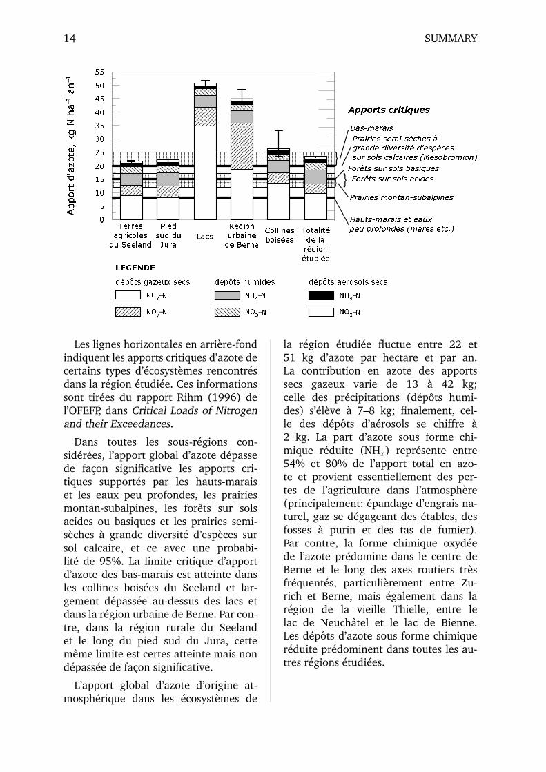
Les lignes horizontales en arriere-fondindiquent les apports critiques d’azote decertains types d’ecosystemes rencontresdans la region etudiee. Ces informationssont tirees du rapport Rihm (1996) del’OFEFP, dans Critical Loads of Nitrogenand their Exceedances.
Dans toutes les sous-regions con-siderees, l’apport global d’azote depassede facon significative les apports cri-tiques supportes par les hauts-maraiset les eaux peu profondes, les prairiesmontan-subalpines, les forets sur solsacides ou basiques et les prairies semi-seches a grande diversite d’especes sursol calcaire, et ce avec une probabi-lite de 95%. La limite critique d’apportd’azote des bas-marais est atteinte dansles collines boisees du Seeland et lar-gement depassee au-dessus des lacs etdans la region urbaine de Berne. Par con-tre, dans la region rurale du Seelandet le long du pied sud du Jura, cettememe limite est certes atteinte mais nondepassee de facon significative.
L’apport global d’azote d’origine at-mospherique dans les ecosystemes de
la region etudiee fluctue entre 22 et51 kg d’azote par hectare et par an.La contribution en azote des apportssecs gazeux varie de 13 a 42 kg;celle des precipitations (depots humi-des) s’eleve a 7–8 kg; finalement, cel-le des depots d’aerosols se chiffre a2 kg. La part d’azote sous forme chi-mique reduite (NHx) represente entre54% et 80% de l’apport total en azo-te et provient essentiellement des per-tes de l’agriculture dans l’atmosphere(principalement: epandage d’engrais na-turel, gaz se degageant des etables, desfosses a purin et des tas de fumier).Par contre, la forme chimique oxydeede l’azote predomine dans le centre deBerne et le long des axes routiers tresfrequentes, particulierement entre Zu-rich et Berne, mais egalement dans laregion de la vieille Thielle, entre lelac de Neuchatel et le lac de Bienne.Les depots d’azote sous forme chimiquereduite predominent dans toutes les au-tres regions etudiees.
SUMMARY 15
Italiano
L’azoto e indispensabile per la cres-cita delle piante e quindi anche perl’alimentazione della popolazione mon-diale. Dato che la forma chimicadell’azoto presente con maggior frequen-za nell’atmosfera (N2) non puo esse-re assimilata direttamente dalle pian-te, nell’agricoltura vengono impiegati, suscala mondiale, ingenti quantitativi difertilizzanti che tendono a ossidare e checontengono forme di azoto ridotte. Nelcorso di parecchie altre attivita umanevengono immessi nell’ambiente, e quin-di anche nell’atmosfera, grandi quanti-tativi di composti d’azoto (NHx) ridottie ossidati (NOx). Dal momento che que-sti composti contribuiscono direttamentead alimentare le piante, comportano an-che un’eutrofizzazione degli ecosistemi.
Gli ecosistemi sono fondamentalmen-te predisposti ad accogliere immissionidi azoto molto minori, le quali proven-gono da microrganismi presenti nel suo-lo che legano l’azoto (trasformando l’N2
presente nell’atmosfera in forme di azotoossidate e ridotte). Si presume percio cheimmissioni supplementari di azoto ossi-dato e ridotto di origine antropica eser-citino un influsso determinante su ecosi-stemi naturali e prossimi allo stato natu-rale. Sintomi di carenza, riduzione dellabiodiversita e cambiamenti nella compo-sizione delle specie degli ecosistemi so-no alcuni degli effetti piu importanti chepossono essere causati dal superamentodei quantitivi critici di immissione (criti-cal loads). Animali e popolazioni di ani-mali che si nutrono di specie di pian-te particolari o che possono essere influ-enzati per altre vie dalla catena alimen-tare complessa, possono essere sensibil-mente disturbati nel loro ambiente natu-rale ed eventualmente scomparire.
Il presente studio esamina il ruo-lo delle immissioni dell’azoto presentenell’atmosfera (deposizione) in una zona
rurale della Svizzera densamente popo-lata che comprende anche piccole citta-dine e paesi piu grandi. E’ incentrato sul-le forme ossidate e ridotte di azoto, manon sull’N2 che costituisce un elemen-to naturale del ciclo dell’azoto. La me-dia annua delle immissioni viene deter-minata per ogni chilometro quadrato diun’area di 50×70 km2. La regione esa-minata comprende il Seeland, parti delGiura e si estende fino alla zona collina-re prealpina a sud di Berna.
Il carico totale delle immissioni e co-stituito dalle tre componenti: (1) deposi-zione secca in forma gassosa, (2) depo-sizione umida (provocata dalla pioggia)e (3) deposizione secca di particelle diaerosol. Per determinare la deposizionesecca di sostanze gassose e stato utiliz-zato un modello elaborato al computer(p. es. ammoniaca NH3, ossido d’azotoNO, biossido d’azoto NO2); la deposizio-ne umida e quella di aerosol sono stateinvece stimate in base ai dati di misura-zioni estrapolate dal punto di vista ter-ritoriale, per quanto concerne l’area esa-minata.
I carichi annui per ogni chilometroquadrato della regione esaminata sonostati riassunti nelle medie regionali diaree parziali scelte (vedi fig. alla pagi-na seguente). Le colonne indicano la me-dia del totale annuo della deposizionedi azoto per ettaro. Le barre verticali re-lative agli errori definiscono l’intervallodi confidenza del 95% delle immissio-ni annue. L’ombreggiatura delle colon-ne indica le relative percentuali di for-me d’azoto ridotte e ossidate dei tre tipidi deposizione considerati nella presentericerca.
Le linee orizzontali sullo sfondo diquesta figura indicano le immissioni cri-tiche di alcuni tipi di ecosistemi scelti,presenti nella regione esaminata. I valo-ri e i settori critici sono stati stabiliti nelrapporto dell’UFAFP di Rihm (1996), inCritical Loads of Nitrogen and their Ex-
16 SUMMARY
��
��������������������
,PPL
VVLRQ
L�GD]
RWR��N
J�1�KD
���DQ
QR��
9HUVDQWHVXG�GHO*LXUD
/DJKL6HHODQG�DJULFROWXUD
$UHDXUEDQDGL�%HUQD
&ROOLQHERVFRVH
$UHDFRPSOHV�
VLYD
}
}}
3DOXGL
%RVFL�VX�WHUUHQL�DFLGL3UDWL�H�SDVFROL�VXEDOSLQLGL�PRQWDJQD
7RUELHUH�DOWH�H�DFTXH�EDVVH��DFTXLWULQL�HFF��
%RVFKL�VX�WHUUHQL�EDVLFL
3UDWL�VHPLVHFFKL�ULFFKL�GLVSHFLH�DQLPDOL�H�YHJHWDOLVX�WHUUHQR�FDOFDUHR�0HVREURPLRQ�
,PPLVVLRQL�FULWLFKH
1+[�112\�1
1+��112��1
1+��112��1
'HSRVL]LRQH�JDVVRVD��VHFFD 'HSRVL]LRQH�XPLGD 'HSRVL]LRQH�GL�SDUWLFHOOH�GL�DHURVRO/(*(1'$
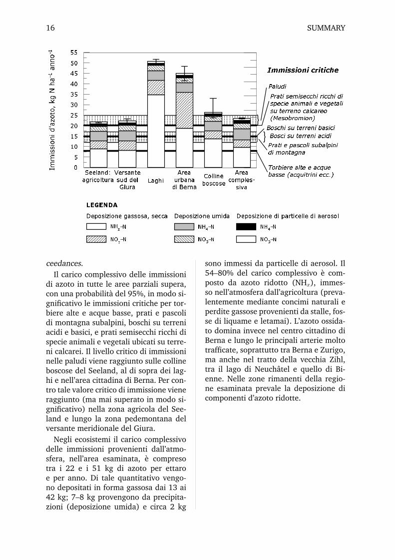
ceedances.Il carico complessivo delle immissioni
di azoto in tutte le aree parziali supera,con una probabilita del 95%, in modo si-gnificativo le immissioni critiche per tor-biere alte e acque basse, prati e pascolidi montagna subalpini, boschi su terreniacidi e basici, e prati semisecchi ricchi dispecie animali e vegetali ubicati su terre-ni calcarei. Il livello critico di immissioninelle paludi viene raggiunto sulle collineboscose del Seeland, al di sopra dei lag-hi e nell’area cittadina di Berna. Per con-tro tale valore critico di immissione vieneraggiunto (ma mai superato in modo si-gnificativo) nella zona agricola del See-land e lungo la zona pedemontana delversante meridionale del Giura.
Negli ecosistemi il carico complessivodelle immissioni provenienti dall’atmo-sfera, nell’area esaminata, e compresotra i 22 e i 51 kg di azoto per ettaroe per anno. Di tale quantitativo vengo-no depositati in forma gassosa dai 13 ai42 kg; 7–8 kg provengono da precipita-zioni (deposizione umida) e circa 2 kg
sono immessi da particelle di aerosol. Il54–80% del carico complessivo e com-posto da azoto ridotto (NHx), immes-so nell’atmosfera dall’agricoltura (preva-lentemente mediante concimi naturali eperdite gassose provenienti da stalle, fos-se di liquame e letamai). L’azoto ossida-to domina invece nel centro cittadino diBerna e lungo le principali arterie moltotrafficate, soprattutto tra Berna e Zurigo,ma anche nel tratto della vecchia Zihl,tra il lago di Neuchatel e quello di Bi-enne. Nelle zone rimanenti della regio-ne esaminata prevale la deposizione dicomponenti d’azoto ridotte.

1. Introduction
Plant growth in most ecosystems of theworld is limited by nitrogen supply. Toincrease yield, the application of ni-trogen fertilizers to agricultural cropshas been practiced ever since mankindmoved from the early stage of huntersand gatherers to agricultural farming.With the rapid growth of the world pop-ulation and the invention of artificial fer-tilizers it was possible to increase agri-cultural yields rapidly to keep pace withthe ever growing food demands of theglobal population. However, as with anyother human activity, some of the fertil-izer applied to agricultural fields neverreach the target plants but instead arevolatilized, and in so doing fertilize theatmosphere rather than the crops.
Agricultural fertilizers are just one ex-ample of nitrogen sources from humanactivities. Other important sources of ni-trogen are all kinds of traffic (especiallymotorized traffic and aircrafts), residen-tial heating and other combustion pro-cesses (human waste incinerators, indus-trial heating). All these sources emit ni-trogen in oxidized (NO, NO2) or reducedform (NH3) that are easily accessible forplant organisms.
1.1 Purpose of the Study
The purpose of this study was to givequantitative estimates of current nitro-gen loads in a rural area of Switzerlandwhere small towns, intensive agricultureand some industry dominate the picture.Thus, within the study area (Chapter 3)automobile traffic was supposed to onlyplay a minor role in current nitrogen
loads.
The focus of our interest was in findingthe link between source locations, wherenitrogen emitted by human activities islost to the atmosphere, and sink loca-tions, where this plant available nitro-gen is input into semi-natural and nat-ural ecosystems.
“Plant available nitrogen” is not welldefined in a scientific sense. With thisterm we refer to all the oxidized and re-duced chemical forms of nitrogen as theyappear in the atmosphere, and whichare potentially available to plant organ-isms. Thus, we exclude molecular nitro-gen (N2)—which makes up roughly 70%of the atmosphere—from our considera-tions, because N2 is not directly accessi-ble to plants due to its chemical form.
However, in reality, fungi and mycor-rhizae on plant roots may trap some ofthe so-called plant available nitrogen fortheir own use and thus make it unavail-able to plants. On the other hand, Rhi-zobium bacteria are able to chemicallyreduce small fractions of molecular ni-trogen (N2). This nitrogen is known tocontribute significantly to plant availablenitrogen pools in ecosystems with greatabundance of alders or legumes, andin regenerating agricultural fields whereclover and other legumes were seededintentionally.
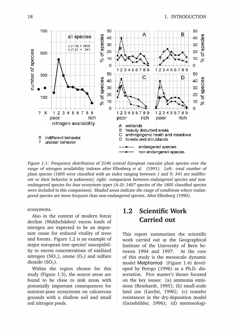
It was shown by Ellenberg (1990) thatmost nutrient-poor ecosystem types dis-play the highest species diversity andthe largest fraction of endangered plantspecies (Figure 1.1) and thus addition ofnutrients, especially nitrogen addition isexpected to have a huge impact on these
17
18 1. INTRODUCTION
AAAAAAAAAAAAAAAAAAAAAAAAAAAAAAAAAAAAAAAAAAAAAAAAAAAAAAAAAAAA
AAAAAAAAAAAAAAAAAAAAAAAAAAAAAAAAAAAAAAAAAAAAAAAAAAAAAAAAAAAA
AAAAAAAAAAAAAAAAAAAAAAAAAAAAAAAAAAAAAAAAAAAAAAAAAAAAAAAAAAAA
AAAAAAAAAAAAAAAAAAAAAAAAAAAAAAAAAAAAAAAAAAAAAAAAAAAAAAAAAAAAAAAAAAAAAAAAAAAAAAAAAAAA
AAAAAAAAAAAAAAAAAAAAAAAAAAAAAAAAAAAAAAAAAAAAAAAAAAAAAAAAAAAAAAAAAAAAAAAAAAAAAAAAAAAA
AAAAAAAAAAAAAAAAAAAAAAAAAAAAAAAAAAAAAAAAAAAAAAAAAAAAAAAAAAAAAAAAAAAAAAAAAAAAAAAAAAAA
AAAAAAAAAAAAAAAAAAAAAAAAAAAAAAAAAAAAAAAAAAAAAAAAAAAAAAAAAAAAAAAAAAAAAAAAAAAAAAAAAAAAAAAAAAAAAAAAAAAA
AAAAAAAAAAAAAAAAAAAAAAAAAAAAAAAAAAAAAAAAAAAAAAAAAAAAAAAAAAAAAAAAAAAAAAAAAAAAAAAAAAAAAAAAAAAAAAAAAAAA
AAAAAAAAAAAAAAAAAAAAAAAAAAAAAAAAAAAAAAAAAAAAAAAAAAAAAAAAAAAAAAAAAAAAAAAAAAAAAAAAAAAAAAAAAAAAAAAAAAAA
AAAAAAAAAAAAAAAAAAAAAAAAAAAAAAAAAAAAAAAAAAAAAAAAAAAAAAAAAAAAAAAAAAAAAAAA
AAAAAAAAAAAAAAAAAAAAAAAAAAAAAAAAAAAAAAAAAAAAAAAAAAAAAAAAAAAAAAAAAAAAAAAA
AAAAAAAAAAAAAAAAAAAAAAAAAAAAAAAAAAAAAAAAAAAAAAAAAAAAAAAAAAAAAAAAAAAAAAAA
1 2 3 4 5 6 7 8 9poor rich nitrogen availability
100
300
500
700
number of species
? X
n (1..9) = 1805n (?,X) = 341
1 2 3 4 5 6 7 8 9poor rich
01020304050
% of species
1 2 3 4 5 6 7 8 9poor rich
01020304050
% of species
1 2 3 4 5 6 7 8 90
1020304050
% of species
1 2 3 4 5 6 7 8 901020304050
% of species
endangered speciesnon endangered species
wetlandsheavily disturbed areasanthropogenic heath and meadowsforests and shrublands
ABCD
A B
C D
all species
indifferent behaviorunclear behavior
X?
Figure 1.1: Frequency distribution of 2146 central European vascular plant species over therange of nitrogen availability indexes after Ellenberg et al. (1991). Left: total number ofplant species (1805 were classified with an index ranging between 1 and 9; 341 are indiffer-ent or their behavior is unknown); right: comparison between endangered species and non-endangered species for four ecosystem types (A–D; 1407 species of the 1805 classified specieswere included in this comparison). Shaded areas indicate the range of conditions where endan-gered species are more frequent than non-endangered species. After Ellenberg (1990).
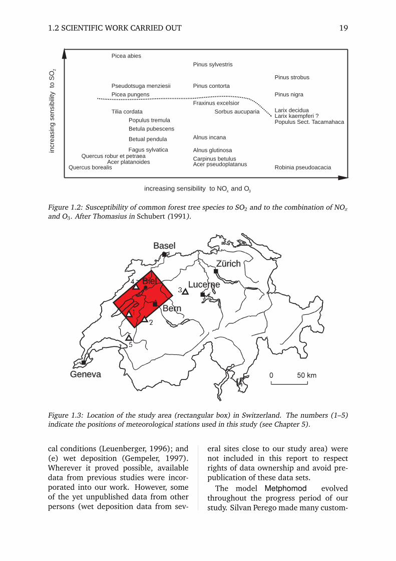
ecosystems.Also in the context of modern forest
decline (Waldschaden) excess loads ofnitrogen are expected to be an impor-tant cause for reduced vitality of treesand forests. Figure 1.2 is an example ofmajor european tree species’ susceptibil-ity to excess concentrations of oxidizednitrogen (NOx), ozone (O3) and sulfuredioxide (SO2).
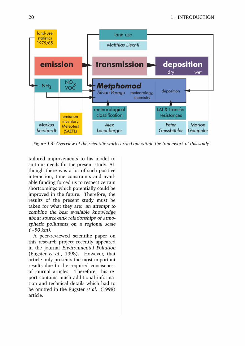
Within the region chosen for thisstudy (Figure 1.3), the source areas arefound to be close to sink areas withpotentially important consequences fornutrient-poor ecosystems on calcareousgrounds with a shallow soil and smallsoil nitrogen pools.
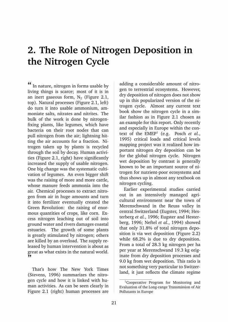
1.2 Scientific WorkCarried out
This report summarizes the scientificwork carried out at the GeographicalInstitute of the University of Bern be-tween 1994 and 1997. At the coreof this study is the mesoscale dynamicmodel Metphomod (Figure 1.4) devel-oped by Perego (1996) as a Ph.D. dis-sertation. Five master’s theses focusedon the key issues: (a) ammonia emis-sions (Reinhardt, 1995); (b) small-scaleland use (Liechti, 1996); (c) transferresistances in the dry-deposition model(Geissbuhler, 1996); (d) meteorologi-
1.2 SCIENTIFIC WORK CARRIED OUT 19
increasing sensibility to NOx and O3
incr
easi
ng s
ensi
bilit
y to
SO
2Picea abies
Pseudotsuga menziesii
Picea pungens
Tilia cordata
Populus tremula
Betula pubescens
Betual pendula
Fagus sylvaticaQuercus robur et petraea
Acer platanoidesQuercus borealis
Pinus sylvestris
Pinus contorta
Fraxinus excelsior
Sorbus aucuparia
Alnus incana
Alnus glutinosa
Carpinus betulusAcer pseudoplatanus
Pinus strobus
Pinus nigra
Larix deciduaLarix kaempferi ?Populus Sect. Tacamahaca
Robinia pseudoacacia
Figure 1.2: Susceptibility of common forest tree species to SO2 and to the combination of NOx
and O3. After Thomasius in Schubert (1991).
Bern
Biel
12
3
5
4
Geneva
Zürich
Basel
Lucerne
Figure 1.3: Location of the study area (rectangular box) in Switzerland. The numbers (1–5)indicate the positions of meteorological stations used in this study (see Chapter 5).
cal conditions (Leuenberger, 1996); and(e) wet deposition (Gempeler, 1997).Wherever it proved possible, availabledata from previous studies were incor-porated into our work. However, someof the yet unpublished data from otherpersons (wet deposition data from sev-
eral sites close to our study area) werenot included in this report to respectrights of data ownership and avoid pre-publication of these data sets.
The model Metphomod evolvedthroughout the progress period of ourstudy. Silvan Perego made many custom-
20 1. INTRODUCTION
Figure 1.4: Overview of the scientific work carried out within the framework of this study.
tailored improvements to his model tosuit our needs for the present study. Al-though there was a lot of such positiveinteraction, time constraints and avail-able funding forced us to respect certainshortcomings which potentially could beimproved in the future. Therefore, theresults of the present study must betaken for what they are: an attempt tocombine the best available knowledgeabout source-sink relationships of atmo-spheric pollutants on a regional scale(∼50 km).
A peer-reviewed scientific paper onthis research project recently appearedin the journal Environmental Pollution(Eugster et al., 1998). However, thatarticle only presents the most importantresults due to the required concisenessof journal articles. Therefore, this re-port contains much additional informa-tion and technical details which had tobe omitted in the Eugster et al. (1998)article.
2. The Role of Nitrogen Deposition inthe Nitrogen Cycle
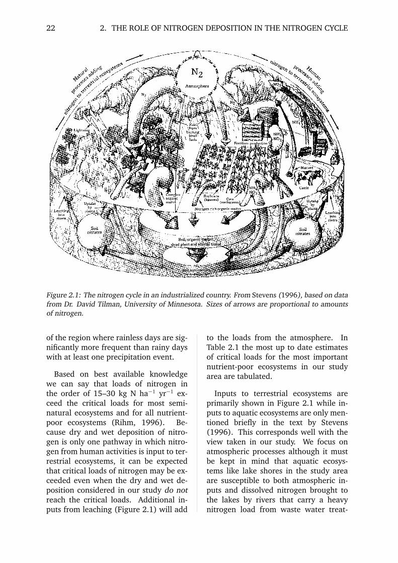
“ In nature, nitrogen in forms usable byliving things is scarce; most of it is inan inert gaseous form, N2 (Figure 2.1,top). Natural processes (Figure 2.1, left)do turn it into usable ammonium, am-moniate salts, nitrates and nitrites. Thebulk of the work is done by nitrogen-fixing plants, like legumes, which havebacteria on their root nodes that canpull nitrogen from the air; lightning hit-ting the air accounts for a fraction. Ni-trogen taken up by plants is recycledthrough the soil by decay. Human activi-ties (Figure 2.1, right) have significantlyincreased the supply of usable nitrogen.One big change was the systematic culti-vation of legumes. An even bigger shiftwas the raising of more and more cattle,whose manure feeds ammonia into theair. Chemical processes to extract nitro-gen from air in huge amounts and turnit into fertilizer eventually created theGreen Revolution: the raising of enor-mous quantities of crops, like corn. Ex-cess nitrogen leaching out of soil intoground water and rivers damages coastalestuaries. The growth of some plantsis greatly stimulated by nitrogen; othersare killed by an overload. The supply re-leased by human intervention is about asgreat as what exists in the natural world.
”That’s how The New York Times
(Stevens, 1996) summarizes the nitro-gen cycle and how it is linked with hu-man activities. As can be seen clearly inFigure 2.1 (right) human processes are
adding a considerable amount of nitro-gen to terrestrial ecosystems. However,dry deposition of nitrogen does not showup in this popularized version of the ni-trogen cycle. Almost any current textbook show the nitrogen cycle in a sim-ilar fashion as in Figure 2.1 chosen asan example for this report. Only recentlyand especially in Europe within the con-text of the EMEP1 (e.g. Posch et al.,1995) critical loads and critical levelsmapping project was it realized how im-portant nitrogen dry deposition can befor the global nitrogen cycle. Nitrogenwet deposition by contrast is generallyknown to be an important source of ni-trogen for nutrient-poor ecosystems andthus shows up in almost any textbook onnitrogen cycling.
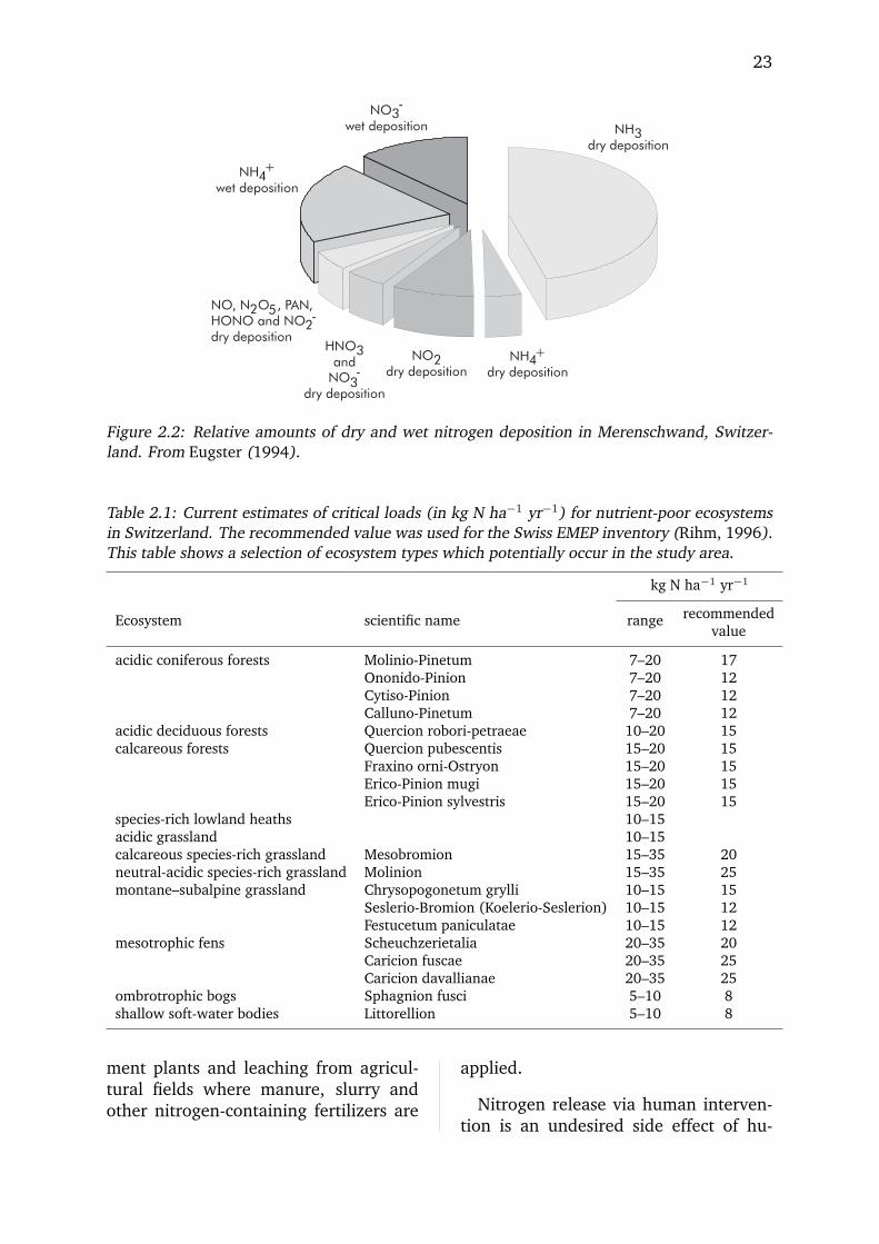
Earlier experimental studies carriedout in an intensively managed agri-cultural environment near the town ofMerenschwand in the Reuss valley incentral Switzerland (Eugster, 1994; Hes-terberg et al., 1996; Eugster and Hester-berg, 1996; Neftel et al., 1994) showedthat only 31.8% of total nitrogen depo-sition is via wet deposition (Figure 2.2)while 68.2% is due to dry deposition.From a total of 28.3 kg nitrogen per haper year at Merenschwand 19.3 kg orig-inate from dry deposition processes and9.0 kg from wet deposition. This ratio isnot something very particular to Switzer-land, it just reflects the climate regime
1Cooperative Program for Monitoring andEvaluation of the Long-range Transmission of AirPollutants in Europe
21
22 2. THE ROLE OF NITROGEN DEPOSITION IN THE NITROGEN CYCLE
Figure 2.1: The nitrogen cycle in an industrialized country. From Stevens (1996), based on datafrom Dr. David Tilman, University of Minnesota. Sizes of arrows are proportional to amountsof nitrogen.
of the region where rainless days are sig-nificantly more frequent than rainy dayswith at least one precipitation event.
Based on best available knowledgewe can say that loads of nitrogen inthe order of 15–30 kg N ha−1 yr−1 ex-ceed the critical loads for most semi-natural ecosystems and for all nutrient-poor ecosystems (Rihm, 1996). Be-cause dry and wet deposition of nitro-gen is only one pathway in which nitro-gen from human activities is input to ter-restrial ecosystems, it can be expectedthat critical loads of nitrogen may be ex-ceeded even when the dry and wet de-position considered in our study do notreach the critical loads. Additional in-puts from leaching (Figure 2.1) will add
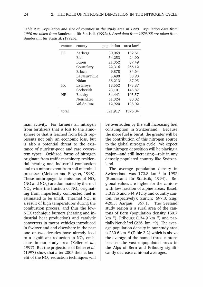
to the loads from the atmosphere. InTable 2.1 the most up to date estimatesof critical loads for the most importantnutrient-poor ecosystems in our studyarea are tabulated.
Inputs to terrestrial ecosystems areprimarily shown in Figure 2.1 while in-puts to aquatic ecosystems are only men-tioned briefly in the text by Stevens(1996). This corresponds well with theview taken in our study. We focus onatmospheric processes although it mustbe kept in mind that aquatic ecosys-tems like lake shores in the study areaare susceptible to both atmospheric in-puts and dissolved nitrogen brought tothe lakes by rivers that carry a heavynitrogen load from waste water treat-
23
Figure 2.2: Relative amounts of dry and wet nitrogen deposition in Merenschwand, Switzer-land. From Eugster (1994).
Table 2.1: Current estimates of critical loads (in kg N ha−1 yr−1) for nutrient-poor ecosystemsin Switzerland. The recommended value was used for the Swiss EMEP inventory (Rihm, 1996).This table shows a selection of ecosystem types which potentially occur in the study area.
kg N ha−1 yr−1
recommendedEcosystem scientific name rangevalue
acidic coniferous forests Molinio-Pinetum 7–20 17Ononido-Pinion 7–20 12Cytiso-Pinion 7–20 12Calluno-Pinetum 7–20 12
acidic deciduous forests Quercion robori-petraeae 10–20 15calcareous forests Quercion pubescentis 15–20 15
Fraxino orni-Ostryon 15–20 15Erico-Pinion mugi 15–20 15Erico-Pinion sylvestris 15–20 15
species-rich lowland heaths 10–15acidic grassland 10–15calcareous species-rich grassland Mesobromion 15–35 20neutral-acidic species-rich grassland Molinion 15–35 25montane–subalpine grassland Chrysopogonetum grylli 10–15 15
Seslerio-Bromion (Koelerio-Seslerion) 10–15 12Festucetum paniculatae 10–15 12
mesotrophic fens Scheuchzerietalia 20–35 20Caricion fuscae 20–35 25Caricion davallianae 20–35 25
ombrotrophic bogs Sphagnion fusci 5–10 8shallow soft-water bodies Littorellion 5–10 8
ment plants and leaching from agricul-tural fields where manure, slurry andother nitrogen-containing fertilizers are
applied.
Nitrogen release via human interven-tion is an undesired side effect of hu-
24 2. THE ROLE OF NITROGEN DEPOSITION IN THE NITROGEN CYCLE
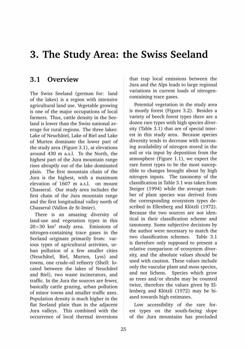
Table 2.2: Population and size of counties in the study area in 1990. Population data from1990 are taken from Bundesamt fur Statistik (1992a). Areal data from 1979/85 are taken fromBundesamt fur Statistik (1992b).
canton county population area km2
BE Aarberg 30,069 152.61Biel 54,253 24.90Buren 21,352 87.49Courtelary 22,316 266.12Erlach 9,878 84.64La Neuveville 5,498 58.98Nidau 38,213 87.95
FR La Broye 18,552 173.87Seebezirk 23,101 145.87
NE Boudry 34,441 105.57Neuchatel 51,324 80.02Val-de-Ruz 12,920 128.02
total 321,917 1396.04
man activity. For farmers all nitrogenfrom fertilizers that is lost to the atmo-sphere or that is leached from fields rep-resents not only an economic loss, butis also a potential threat to the exis-tance of nutrient-poor and rare ecosys-tem types. Oxidized forms of nitrogenoriginate from traffic machinery, residen-tial heating and industrial combustionand to a minor extent from soil microbialprocesses (Meixner and Eugster, 1998).These anthropogenic emissions of NOx
(NO and NO2) are dominated by thermalNOx while the fraction of NOx originat-ing from imperfectly combusted fuel isestimated to be small. Thermal NOx isa result of high temperatures during thecombustion process, and thus the low-NOX technique burners (heating and in-dustrial heat production) and catalyticconverters in motor vehicles introducedin Switzerland and elsewhere in the pastone or two decades have already leadto a significant reduction in NOx emis-sions in our study area (Keller et al.,1997). But the projections of Keller et al.(1997) show that after 2005 the net ben-efit of the NOx reduction techniques will
be overridden by the still increasing fuelconsumption in Switzerland. Becausethe more fuel is burnt, the greater will bethe contribution of this nitrogen sourceto the global nitrogen cycle. We expectthat nitrogen deposition will be playing amajor—and still increasing—role in anydensely populated country like Switzer-land.
The average population density inSwitzerland was 172.8 km−2 in 1992(Bundesamt fur Statistik, 1994). Re-gional values are higher for the cantonswith low fraction of alpine areas: Basel:5,313.5 and 544.9 (city and country can-ton, respectively); Zurich: 697.3; Zug:420.5, Aargau: 367.1. The Seelandstudy region is a rural area of the can-tons of Bern (population density 160.7km−2), Fribourg (134.9 km−2) and par-tially Neuchatel (226. km−29). The aver-age population density in our study areais 230.6 km−2 (Table 2.2) which is abovethe average of the named three cantonsbecause the vast unpopulated areas inthe Alps of Bern and Fribourg signifi-cantly decrease cantonal averages.
3. The Study Area: the Swiss Seeland
3.1 Overview
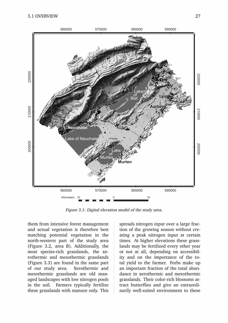
The Swiss Seeland (german for: landof the lakes) is a region with intensiveagricultural land use. Vegetable growingis one of the major occupations of localfarmers. Thus, cattle density in the See-land is lower than the Swiss national av-erage for rural regions. The three lakes:Lake of Neuchatel, Lake of Biel and Lakeof Murten dominate the lower part ofthe study area (Figure 3.1), at elevationsaround 430 m a.s.l. To the North, thehighest part of the Jura mountain rangerises abruptly out of the lake dominatedplain. The first mountain chain of theJura is the highest, with a maximumelevation of 1607 m a.s.l. on mountChasseral. Our study area includes thefirst chain of the Jura mountain rangeand the first longitudinal valley north ofChasseral (Vallon de St-Imier).
There is an amazing diversity ofland-use and vegetation types in this20×30 km2 study area. Emissions ofnitrogen-containing trace gases in theSeeland originate primarily from: var-ious types of agricultural activities, ur-ban pollution of a few smaller cities(Neuchatel, Biel, Murten, Lyss) andtowns, one crude-oil refinery (Shell: lo-cated between the lakes of Neuchateland Biel), two waste incinerators, andtraffic. In the Jura the sources are fewer,basically cattle grazing, urban pollutionof minor towns and smaller traffic axes.Population density is much higher in theflat Seeland plain than in the adjacentJura valleys. This combined with theoccurrence of local thermal inversions
that trap local emissions between theJura and the Alps leads to large regionalvariations in current loads of nitrogen-containing trace gases.
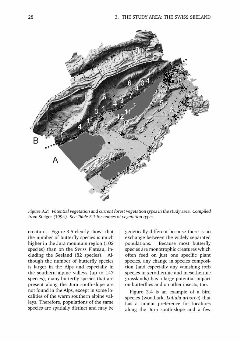
Potential vegetation in the study areais mostly forest (Figure 3.2). Besides avariety of beech forest types there are adozen rare types with high species diver-sity (Table 3.1) that are of special inter-est in this study area. Because speciesdiversity tends to decrease with increas-ing availability of nitrogen stored in thesoil or via input by deposition from theatmosphere (Figure 1.1), we expect therare forest types to be the most suscep-tible to changes brought about by highnitrogen inputs. The taxonomy of theclassification in Table 3.1 was taken fromSteiger (1994) while the average num-ber of plant species was derived fromthe corresponding ecosystem types de-scribed in Ellenberg and Klotzli (1972).Because the two sources are not iden-tical in their classification scheme andtaxonomy. Some subjective decisions bythe author were necessary to match thetwo classification schemes. Table 3.1is therefore only supposed to present arelative comparison of ecosystem diver-sity, and the absolute values should beused with caution. These values includeonly the vascular plant and moss species,and not lichens. Species which growas trees and/or shrubs may be countedtwice, therefore the values given by El-lenberg and Klotzli (1972) may be bi-ased towards high estimates.
Low accessibility of the rare for-est types on the south-facing slopeof the Jura mountains has precluded
25

26 3. THE STUDY AREA: THE SWISS SEELAND
Table 3.1: Species diversity of forest types found in the study area. The codes A, B, and 1–12refer to Figure 3.2. The values are the average number of plant species in a given ecosystemtype. Higher values indicate species-rich ecosystems (high species diversity), low values aretypical for monocultural agro-ecosystems. See text for details.
avg. numberCode german name scientific nameof plant species
A Beech forests at lower elevations of the Seeland 40.4Weissmoos-Buchenwald Luzulo silvaticae-Fagetum
leucobryetosum27.2
Waldhainsimsen-Buchenwald Luzulo silvaticae-Fagetumtypicum
36.2
Traubenkirschen-Eschenmischwald Pruno-Fraxinetum 39.4Waldmeister-Buchenwald Galio odorati-Fagetum
typicum40.4
Aronstab-Buchenwald Aro-Fagetum 43.6Immenblatt-Buchenwald Pulmonario-Fagetum
melittetosum andLathyro-Fagetum caricetosum
47.4
Lungenkraut-Buchenwald Pulmonario-Fagetum typicumand Lathyro-Fagetumtypicum
48.7
B Beech, maple and fir forests in the Jura mountains 43.9Tannen-Buchenwald (various types) Abieti-Fagetum 32.7–52.7Hirschzungen-Ahornwald Phyllitido-Aceretum 34.4Linden-Buchenwald 39.3Alpendost-Buchenwald 39.3Zahnwurz-Buchenwald Dentario-Fagetum typicum 42.1Blaugras-Buchenwald Seslerio-Fagetum 49.0Eiben-Buchenwald Taxo-Fagetum 50.0Weisseggen-Buchenwald Carici albae-Fagetum typicum 55.3
1 Platterbsen-Traubeneichenwald Lathyro-Quercetum 64.02 Schachtelhalm-Tannen-Fichtenwald Equiseto-Abieti-Piceetum 58.53 Strauchkronwicken-Flaumeichenwald Coronillo-Quercetum 51.5–57.14 Ahorn-Sommerlindenwald Aceri-Tilietum 55.35 Stieleichen-Hagebuchenmischwald Querco-Carpinetum 55.16 Ahorn-Buchenwald Aceri-Fagetum 45.87 Mehlbeer-Ahornwald Sorbo-Aceretum 42.48 Ulmen-Eschenauenwald Ulmo-Fraxinetum typicum 36.99 Kronwicken-Fohrenwald Coronillo-Pinetum 34.010 Silberweiden-Auenwald Salicetum albae 30.311 Seggen-Schwarzerlenbruch Carici elongatae-Alnetum
glutionsae27.1
12 Fohren-Birkenbruch Pino-Betuletum pubescentis 23.9— Ahorn-Eschenwald (on moist soils) Aceri-Fraxinetum 50.0
3.1 OVERVIEW 27
Lake of Neuchatel
Lakeof
Murten
Lakeof
BielLyss
Aarberg
Neuchatel
Biel
Murten
010Kilometers 10
560000200000 2
00000
210000 2
10000
220000 2
20000
560000
570000
570000
580000
580000
590000
590000
Figure 3.1: Digital elevation model of the study area.
them from intensive forest managementand actual vegetation is therefore bestmatching potential vegetation in thenorth-western part of the study area(Figure 3.2, area B). Additionally, themost species-rich grasslands, the xe-rothermic and mesothermic grasslands(Figure 3.3) are found in the same partof our study area. Xerothermic andmesothermic grasslands are old man-aged landscapes with low nitrogen poolsin the soil. Farmers typically fertilizethese grasslands with manure only. This
spreads nitrogen input over a large frac-tion of the growing season without cre-ating a peak nitrogen input at certaintimes. At higher elevations these grass-lands may be fertilized every other yearor not at all, depending on accessibil-ity and on the importance of the to-tal yield to the farmer. Forbs make upan important fraction of the total abun-dance in xerothermic and mesothermicgrasslands. Their color-rich blossoms at-tract butterflies and give an extraordi-narily well-suited environment to these
28 3. THE STUDY AREA: THE SWISS SEELAND
B
A
34
1211
10
5
8
6
13
6 34
5
9
4
2
7
10
41
Figure 3.2: Potential vegetation and current forest vegetation types in the study area. Compiledfrom Steiger (1994). See Table 3.1 for names of vegetation types.
creatures. Figure 3.5 clearly shows thatthe number of butterfly species is muchhigher in the Jura mountain region (102species) than on the Swiss Plateau, in-cluding the Seeland (82 species). Al-though the number of butterfly speciesis larger in the Alps and especially inthe southern alpine valleys (up to 147species), many butterfly species that arepresent along the Jura south-slope arenot found in the Alps, except in some lo-calities of the warm southern alpine val-leys. Therefore, populations of the samespecies are spatially distinct and may be
genetically different because there is noexchange between the widely separatedpopulations. Because most butterflyspecies are monotrophic creatures whichoften feed on just one specific plantspecies, any change in species composi-tion (and especially any vanishing forbspecies in xerothermic and mesothermicgrasslands) has a large potential impacton butterflies and on other insects, too.
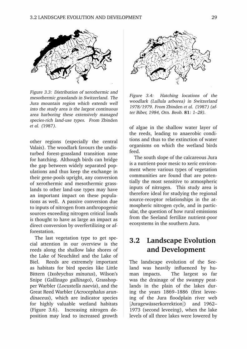
Figure 3.4 is an example of a birdspecies (woodlark, Lullula arborea) thathas a similar preference for localitiesalong the Jura south-slope and a few
3.2 LANDSCAPE EVOLUTION AND DEVELOPMENT 29
Figure 3.3: Distribution of xerothermic andmesothermic grasslands in Switzerland. TheJura mountain region which extends wellinto the study area is the largest continuousarea harboring these extensively managedspecies-rich land-use types. From Zbindenet al. (1987).
other regions (especially the centralValais). The woodlark favours the undis-turbed forest-grassland transition zonefor hatching. Although birds can bridgethe gap between widely separated pop-ulations and thus keep the exchange intheir gene-pools upright, any conversionof xerothermic and mesothermic grass-lands to other land-use types may havean important impact on these popula-tions as well. A passive conversion dueto inputs of nitrogen from anthropogenicsources exceeding nitrogen critical loadsis thought to have as large an impact asdirect conversion by overfertilizing or af-forestation.
The last vegetation type to get spe-cial attention in our overview is thereeds along the shallow lake shores ofthe Lake of Neuchatel and the Lake ofBiel. Reeds are extremely importantas habitats for bird species like LittleBittern (Ixobrychus minutus), Wilson’sSnipe (Gallinago gallinago), Grasshop-per Warbler (Locustella naevia), and theGreat Reed Warbler (Acrocephalus arun-dinaceus), which are indicator speciesfor highly valuable wetland habitats(Figure 3.6). Increasing nitrogen de-position may lead to increased growth
Figure 3.4: Hatching locations of thewoodlark (Lullula arborea) in Switzerland1978/1979. From Zbinden et al. (1987) (af-ter Biber, 1984, Orn. Beob. 81: 1–28).
of algae in the shallow water layer ofthe reeds, leading to anaerobic condi-tions and thus to the extinction of waterorganisms on which the wetland birdsfeed.
The south slope of the calcareous Jurais a nutrient-poor mesic to xeric environ-ment where various types of vegetationcommunities are found that are poten-tially the most sensitive to atmosphericinputs of nitrogen. This study area istherefore ideal for studying the regionalsource-receptor relationships in the at-mospheric nitrogen cycle, and in partic-ular, the question of how rural emissionsfrom the Seeland fertilize nutrient-poorecosystems in the southern Jura.
3.2 Landscape Evolutionand Development
The landscape evolution of the See-land was heavily influenced by hu-man impacts. The largest so farwas the drainage of the swampy peat-lands in the plain of the lakes dur-ing the years 1869–1886 (first levee-ing of the Jura floodplain river web[Juragewasserkorrektion]) and 1962–1973 (second leveeing), when the lakelevels of all three lakes were lowered by

30 3. THE STUDY AREA: THE SWISS SEELAND
Figure 3.5: Butterfly species in Switzerland (daytime active species only). Circles: number ofspecies by primary zones; squares: number of species that occur in two primary zones. Primaryzones: J Jura mountains; M Swiss Plateau (Mittelland); N Northern Alps; V Valais; G Grisons;S Southern Switzerland; E Engadine region. From SBN (1987).
Figure 3.6: Distribution of indicator bird species for highly valuable wetland habitats in Switzer-land. Indicator species used to define valuable wetland habitats are: Little Bittern (Ixobrychusminutus), Wilson’s Snipe (Gallinago gallinago), Grasshopper Warbler (Locustella naevia), andGreat Reed Warbler (Acrocephalus arundinaceus). From Zbinden et al. (1987)

3.3 LAND USE IN 1994 31
10 km
��BB
N
Figure 3.7: Landsat TM satellite image from 4 August 1994 used for land-use classification ofthe year 1994. From Liechti (1996).
roughly 2 m, and a flood protection sys-tem was built with channels between thelakes. It is possible that the deviation ofthe Aare river, which used to flood mostof the lower Seeland rather frequentlyhad the strongest effect on regional cli-mate and thus on the small-scale meteo-rological conditions that control the dis-persion, turbulent transport, and dry de-position of atmospheric trace gases. Be-fore the corrections, the Aare river joinedthe outflow of the Lake of Biel severalkilometers east of the city of Biel be-fore the corrections. Nowadays, the Aareriver enters the Lake of Biel. Thereforethe lake now acts as a buffer for high wa-ters. This deviation of the Aare river pre-vented the Seeland region from flood-
ing. With the new land claimed for agri-culture, local farmers transformed theSeeland into one of the most productiveagricultural regions of Switzerland.
Today, changes in land use are primar-ily due to alterations in farming equip-ment and crop types, and the continu-ing urbanization in the vicinity of citiesand larger towns. Therefore, we decidedto take the land use pattern of the year1994 as a reference for our study.
3.3 Land Use in 1994
As a basis for this study, MatthiasLiechti produced a land-use classification(Liechti, 1996) for the year 1994 usingfour Landsat Thematic Mapper scenes
32 3. THE STUDY AREA: THE SWISS SEELAND
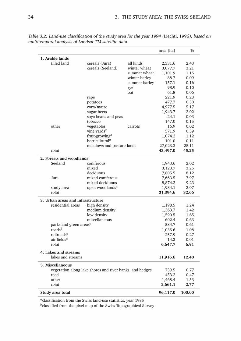
from 30 April, 17 June, 3 July and4 August 1994 (Fig. 3.7). These fourscenes cover most of the growing season(mid April to end of October) and allowa multitemporal-multispectral classifica-tion. This method is capable of resolvingcrops or vegetation types that have sim-ilar spectral properties at one time, buthave different phenology and thus dif-ferent spectral properties at other times(particularly in the early or late grow-ing season). The aim of Liechti’s workwas not only the validation of older sta-tistical land-use data, but also to deter-mine the level of resolution that couldbe achieved by a combination of satel-lite imagery and (typically much older)maps and federal statistics.
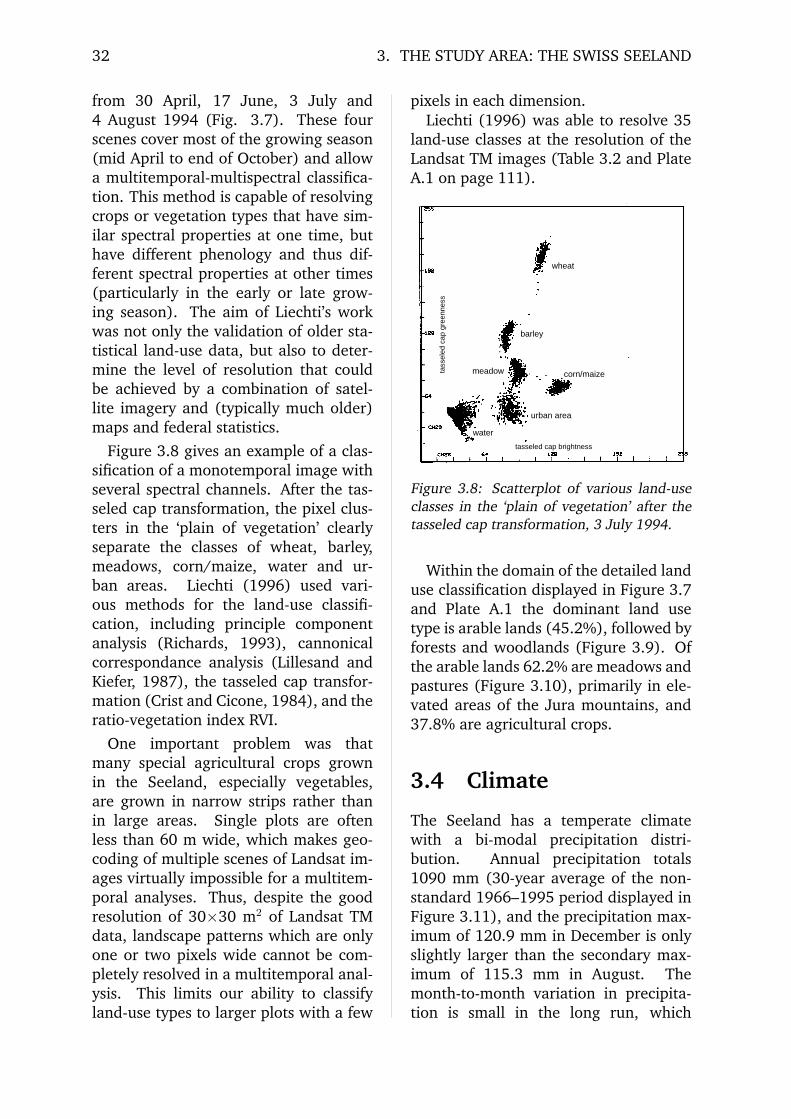
Figure 3.8 gives an example of a clas-sification of a monotemporal image withseveral spectral channels. After the tas-seled cap transformation, the pixel clus-ters in the ‘plain of vegetation’ clearlyseparate the classes of wheat, barley,meadows, corn/maize, water and ur-ban areas. Liechti (1996) used vari-ous methods for the land-use classifi-cation, including principle componentanalysis (Richards, 1993), cannonicalcorrespondance analysis (Lillesand andKiefer, 1987), the tasseled cap transfor-mation (Crist and Cicone, 1984), and theratio-vegetation index RVI.
One important problem was thatmany special agricultural crops grownin the Seeland, especially vegetables,are grown in narrow strips rather thanin large areas. Single plots are oftenless than 60 m wide, which makes geo-coding of multiple scenes of Landsat im-ages virtually impossible for a multitem-poral analyses. Thus, despite the goodresolution of 30×30 m2 of Landsat TMdata, landscape patterns which are onlyone or two pixels wide cannot be com-pletely resolved in a multitemporal anal-ysis. This limits our ability to classifyland-use types to larger plots with a few
pixels in each dimension.Liechti (1996) was able to resolve 35
land-use classes at the resolution of theLandsat TM images (Table 3.2 and PlateA.1 on page 111).
wheat
barley
tass
eled
cap
gre
enne
sstasseled cap brightness
meadow corn/maize
urban area
water
Figure 3.8: Scatterplot of various land-useclasses in the ‘plain of vegetation’ after thetasseled cap transformation, 3 July 1994.
Within the domain of the detailed landuse classification displayed in Figure 3.7and Plate A.1 the dominant land usetype is arable lands (45.2%), followed byforests and woodlands (Figure 3.9). Ofthe arable lands 62.2% are meadows andpastures (Figure 3.10), primarily in ele-vated areas of the Jura mountains, and37.8% are agricultural crops.
3.4 Climate
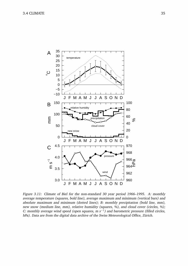
The Seeland has a temperate climatewith a bi-modal precipitation distri-bution. Annual precipitation totals1090 mm (30-year average of the non-standard 1966–1995 period displayed inFigure 3.11), and the precipitation max-imum of 120.9 mm in December is onlyslightly larger than the secondary max-imum of 115.3 mm in August. Themonth-to-month variation in precipita-tion is small in the long run, which

3.4 CLIMATE 33
6.9%
12.4% 2.8%
45.2%
32.7%Figure 3.9: Land-use classification for the year 1994.
2.5%4.5%
11.4%
15.9%
1.3% 1.1%1.1%
62.2%
Figure 3.10: Classification of arable lands for the year 1994.
34 3. THE STUDY AREA: THE SWISS SEELAND
Table 3.2: Land-use classification of the study area for the year 1994 (Liechti, 1996), based onmultitemporal analysis of Landsat TM satellite data.
area [ha] %
1. Arable landstilled land cereals (Jura) all kinds 2,331.6 2.43
cereals (Seeland) winter wheat 3,077.7 3.21summer wheat 1,101.9 1.15winter barley 88.7 0.09summer barley 157.1 0.16rye 98.9 0.10oat 61.8 0.06
rape 221.9 0.23potatoes 477.7 0.50corn/maize 4,977.5 5.17sugar beets 1,943.7 2.02soya beans and peas 24.1 0.03tobacco 147.0 0.15
other vegetables carrots 16.9 0.02vine yardsa 571.9 0.59fruit-growinga 1,074.2 1.12horticulturala 101.0 0.11meadows and pasture-lands 27,023.3 28.11
total 43,497.0 45.25
2. Forests and woodlandsSeeland coniferous 1,943.6 2.02
mixed 3,123.7 3.25deciduous 7,805.5 8.12
Jura mixed coniferous 7,663.5 7.97mixed deciduous 8,874.2 9.23
study area open woodlandsa 1,984.1 2.07total 31,394.6 32.66
3. Urban areas and infrastructureresidential areas high density 1,198.5 1.24
medium density 1,363.7 1.42low density 1,590.5 1.65miscellaneous 602.4 0.63
parks and green areasa 584.7 0.61roadsb 1,035.6 1.08railroadsa 257.9 0.27air fieldsa 14.3 0.01total 6,647.7 6.91
4. Lakes and streamslakes and streams 11,916.6 12.40
5. Miscellaneousvegetation along lake shores and river banks, and hedges 739.5 0.77reed 453.2 0.47other 1,468.4 1.53total 2,661.1 2.77
Study area total 96,117.0 100.00
aclassification from the Swiss land-use statistics, year 1985bclassified from the pixel map of the Swiss Topographical Survey
3.4 CLIMATE 35
J F M A M J J A S O N D−10
−505
101520253035
o C
J F M A M J J A S O N D0
50
100
150
mm
J F M A M J J A S O N D3.0
3.5
4.0
4.5
m s
−1
0
20
40
60
80
100
%
960
962
964
966
968
970
hPa
pressure
wind
new snow
precipitation
cloud cover
relative humidity
temperature
A
B
C
Figure 3.11: Climate of Biel for the non-standard 30 year period 1966–1995. A: monthlyaverage temperature (squares, bold line), average maximum and minimum (vertical bars) andabsolute maximum and minimum (dotted lines); B: monthly precipitation (bold line, mm),new snow (medium line, mm), relative humidity (squares, %), and cloud cover (circles, %);C: monthly average wind speed (open squares, m s−1) and barometric pressure (filled circles,hPa). Data are from the digital data archive of the Swiss Meteorological Office, Zurich.
36 3. THE STUDY AREA: THE SWISS SEELAND
is favorable for agriculture. However,in individual years, the variation insummer and early fall precipitation canseverely affect agricultural crops, partic-ularly during wet years. Droughts arebuffered by the Aare river which orig-inates in the Bernese Alps, and whichfeeds the ground water body in theporous fluvial and glacial deposits inthe lower Seeland region. The 30-year average temperature ranges be-tween 0.10◦C in January and 19.01◦C inJuly (data from the climate station inBiel, Figure 3.11A), with an annual aver-age of 9.23◦C. Absolute maximum tem-perature hardly ever exceeds 30◦C. InBiel, the absolute maximum temperaturerecorded was 30.70◦C, whilst the abso-lute minimum temperature was -7.90◦C,a value that reflects the proximity of theclimate station to the lakes. However,colder minimum temperatures are foundin the lower parts of the Seeland at dis-tances further from the lakes.
A typical climate feature of the See-land is the extensive fogginess which ismost frequent during the winter period(October to March; Wanner, 1979). InFigure 3.11B the fogginess can be seenin the annual cycles of mean relative hu-midity and cloud cover (by definition,fog is also included in the cloudinesstime series of a climate station).
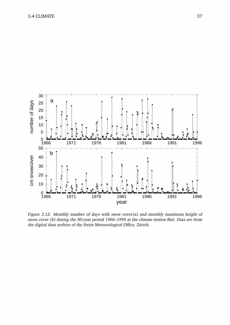
May to October were snowfree inthe 30-year period 1966–1995 (Figure3.11B), and snowfall is only a minor con-tribution to total precipitation even dur-ing the winter months at low altitudes.One of the most dramatic changes inthe past 30 years was the decrease inthe number of days with a snow coverduring the winter (Figure 3.12). There-fore it is important to know that thetime period used in this study to modelnitrogen deposition represents a win-ter situation of only a few days withsnow cover and very little precipitationfalling in the form of snow. However,
frozen soils occurred frequently duringhigh pressure conditions with dense fogor clear sky with no precipitation. Fig-ure 3.11C clearly indicates the frequentoccurrence of high pressure conditionsbetween June and January. The springseason (February to May) reflects thepassage of “April storms”, cyclones withhigh wind speeds and low pressure. Thehigh pressure conditions come in twovariants: during the fall season (Au-gust to October) high pressure is cor-related with low wind speeds. Theseare the conditions with the local name“Altweibersommer”1, where warm daysseem to extend the late summer well intothe fall season, despite cold nights. FromNovember to January, high pressure typ-ically correlates with dense (morning)fog in the Seeland region. The higherwind speeds are related to the “Bise”,the channeled northeasterly flow be-tween the Jura and the Alps (Wannerand Furger, 1990). There are also twovariants of the “Bise”: one which bringscold and clear air from continental re-gions, the other which brings dense fogin lower regions below approximately650–1000 m a.s.l. (“la bise noire”2).
1comparable to the Indian Summer in NorthAmerica.
2french for: the black Bise
3.4 CLIMATE 37
1966 1971 1976 1981 1986 1991 1996year
0
10
20
30
40
50
cm s
now
cove
r
1966 1971 1976 1981 1986 1991 1996 0
5
10
15
20
25
30
num
ber
of d
ays a
b
Figure 3.12: Monthly number of days with snow cover(a) and monthly maximum height ofsnow cover (b) during the 30-year period 1966–1995 at the climate station Biel. Data are fromthe digital data archive of the Swiss Meteorological Office, Zurich.
4. Modeling Approach
4.1 Overview
The core of this study is the dry deposi-tion modeling with Metphomod. In thischapter we present the basics of Met-phomod and elucidate the strengths andweaknesses of this model for the presentpurpose of nitrogen deposition model-ing.
Metphomod was developed by SilvanPerego (1996) for the purpose of mod-eling summer smog conditions, the pri-mary objective of the Pollumet1 project(Neininger and Dommen, 1996). Met-phomod is one of the first models of itskind which links the atmospheric mod-eling of meteorological conditions dy-namically with concurrent chemical re-actions of trace gases in the atmospherethat belong to the well-described but stillnot fully understood photochemical cy-cle during summer smog conditions.
Ozone (O3) is of primary interest inthe context of summer smog. Its pre-cursors include the bulk of the most im-portant nitrogen-containing trace gaseslike NO, NO2, NO3, HNO3, and thus Met-phomod is a valuable tool to model notonly the concentration and distributionof ozone in a region, but also the fluxesand deposition of nitrogen as well.
4.2 Model Design
Metphomod is a three-dimensional dy-namical mesoscale model of the Euleriantype. This compact definition character-
1Pollution and Meteorology of the SwissPlateau
izes some of the most important featuresof this model:
• The model domain, which is the ex-tent of the region to be modeled,is expressed in a three-dimensionalEulerian coordinate system. In ourapplication the horizontal extent ofthe domain was 70×50 km2 with 22vertical layers. The horizontal reso-lution was 1×1 km2 and the verticalspacing between layers was 100 mbetween 450 and 2650 m a.s.l.
• A dynamical model is one that mod-els the physical processes in the at-mosphere based on the primitiveequations of fluid dynamics. Insidethe model domain, every cell hasfour neighbors in the horizontal andtwo neighbors in the vertical dimen-sion. The model basically calculatesall interactions between any cell andits adjacent neighbors that lie withinthe model domain.
• The primitive equations used in themodel are prognostic2 equations,which means that the model knowsthe current state of every variablein the model (e.g concentration of atrace gas) and how it develops overtime. Thus, prognostic calculationsfor every variable can be performed.
• Mesoscale is a meteorological termand describes the scale for which themodel is designed. This corresponds
2prognostic means by definition that a predic-tion in time is possible
38
4.3 MODEL DOMAIN 39
to a domain of a few to a few hun-dred kilometers in the horizontal di-mension, and a few hundred to afew thousand meters in the verticaldimension.
The interactions between the individ-ual cells of the model domain are com-puted at the appropriate time step. Theinteractions are fluxes between two ad-jacent cells, and the chemical reactionsthat occur during one time step interval.Metphomod uses a variable time step of1, 2, 3, 5, 10, 15, 20, 30 or 40 seconds3
for meteorological variables (wind, tem-perature, humidity,...), and a fixed timestep of 120 seconds for chemical reac-tions.
Technical details about Metphomodwere published by Perego (1996), how-ever only in German4. Therefore wefeel that some additional detailed infor-mation is necessary here to describe themodel concept to people who don’t haveaccess to the German language.
The variable time step for meteoro-logical variables allows the computerto match the time scale of the modelwith the time scale of atmospheric tur-bulence, which is a function of horizon-tal wind speed. This saves computingtime, one of the limiting factors in sucha model study. If meteorological con-ditions are persistent, a large time stepstill adequately represents the develop-ment of the atmosphere over time, whileduring quick transitions like frontal pas-sages a time step as short as possible isrequired.
None of the time steps given herefully resolve atmospheric turbulence.Therefore, Metphomod uses the tran-silient turbulence closure scheme byStull (1988) to model the turbulent ex-change between cells which occurs on
3these are the settings used in this project, butthey can be defined freely
4a scientific article by Perego (1999) is ac-cepted for publication
shorter time scales than the one definedby the actual time step.
The atmospheric chemistry is imple-mented with an improved RADM mech-anism (Stockwell, 1986). The versionused in Metphomod knows 39 sub-stances and 82 chemical reactions. Weadded NH3 to this set, because it doesn’tbelong to the photochemical cycle, but isthe most important trace gas in the studyregion in terms of dry deposition. RADMuses the “lumped molecules” concept:similar chemical species which are alsosimilar in reactivity are aggregated intoclasses which are treated like one singlechemical species in the model. This al-lows a significant reduction in the num-ber of substances and reactions requir-ing direct consideration. The numberof substances included is one of the keylimiting factors in this kind of modeling,because computing time increases expo-nentially with each additional substance.
4.3 Model Domain
At first we intended to model the See-land region at as small a horizontal res-olution as possible. However, the timescale of chemical reactions in the pol-luted atmosphere requires a model do-main which is large enough so as to haveallowed all chemical reactions to haveachieved near steady steady state condi-tions by the time the wind moves the airacross the model domain. After some tri-als we ended up with a model domain of50×70 km2 where the region of interest(20×30 km2) is embedded (Figure 5.1).
Grid cell size was 1×1 km2 andthe thickness of the vertical layers was100 m. This gives rise to a new questionas to how to best represent topographywith such a large vertical spacing. Met-phomod inserts an additional interme-diate grid cell with its center 10 m abovethe topography of the digital elevation

40 4. MODELING APPROACH
model. With this special feature of Met-phomod, turbulent transport and mix-ing can still be resolved satisfactorily onmountain slopes and where model layerspoorly agree with local topography.
4.4 Boundary Conditions
Boundary conditions are one of the mostlimiting factors in modeling (both ingeneral and currently, despite the highcomplexity of the model). The idiom“garbage in—garbage out” brings thisneatly to the point and describes thevalue of a numerical model: without ad-equate input (at the borders of a model),the output will not be any better than theinput.
The model has six boundaries: the top,the bottom and the four sides of the box-like model domain. Metphomod’s mete-orology is basically driven by the hori-zontal pressure gradient defined at themodel top. The bottom is defined by thetopography. No wind may penetrate theground, but temperature, humidity andtrace gases interact with the surface intwo ways:
1. Flux from the surface to the atmo-sphere. This can be
• defined by an emission inven-tory (which can have temporalresolution). This approach isused for all trace gases in Met-phomod.
• defined by physical processeslike the absorption of solar ra-diation at the surface which istransformed into ground heatflux, latent heat flux and sensi-ble heat flux. Latent heat fluxbrings moisture from the soilinto the atmosphere, and sen-sible heat flux rises the temper-ature of the atmosphere. Heat
flux from the ground to the at-mosphere lowers the tempera-ture of the soil. These fluxeswhich interact with the atmo-sphere are computed by themodel and depend primarily onthe land-use, vegetation andsoil properties which are inputto the model in the same wayas emission inventories. So-lar position is computed in themodel using empirical astro-nomical equations.
2. Deposition from the atmosphere tothe surface. Deposition—or down-ward flux—is computed by themodel. Heat fluxes are treated in asimilar way for both downward andupward fluxes. However, dry depo-sition is modeled with a resistancemodel, which will be described inSection 4.5.
The four sides of the model can betreated in several ways. We used the ap-proach where the one or two sides fromwhich the mean wind is originating re-quire predefined background concentra-tions of all variables (derived from theEuropean EMEP emission inventory) andthe other sides are passive, i.e. allow theloss of trace gases out of the model do-main at a rate defined by the wind speedand the local concentrations at the bor-der.
4.5 Deposition Module
The deposition module of Metpho-mod calculates the deposition flux oftrace gases based on the concentra-tion gradient between the lowest gridcell and the concentration at roughnesslength z0, in analogy to Fick’s law of dif-fusion. The concentration gradient is thedriving force and a chain of tree resistorsRa, Rb, and Rc (Figure 4.1) determine
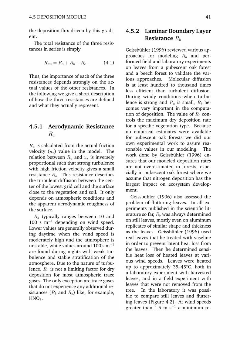
4.5 DEPOSITION MODULE 41
the deposition flux driven by this gradi-ent.
The total resistance of the three resis-tances in series is simply
Rtot = Ra +Rb +Rc . (4.1)
Thus, the importance of each of the threeresistances depends strongly on the ac-tual values of the other resistances. Inthe following we give a short descriptionof how the three resistances are definedand what they actually represent.
4.5.1 Aerodynamic ResistanceRa
Ra is calculated from the actual frictionvelocity (u∗) value in the model. Therelation between Ra and u∗ is inverselyproportional such that strong turbulencewith high friction velocity gives a smallresistance Ra. This resistance describesthe turbulent diffusion between the cen-ter of the lowest grid cell and the surfaceclose to the vegetation and soil. It onlydepends on atmospheric conditions andthe apparent aerodynamic roughness ofthe surface.Ra typically ranges between 10 and
100 s m−1 depending on wind speed.Lower values are generally observed dur-ing daytime when the wind speed ismoderately high and the atmosphere isunstable, while values around 100 s m−1
are found during nights with weak tur-bulence and stable stratification of theatmosphere. Due to the nature of turbu-lence, Ra is not a limiting factor for drydeposition for most atmospheric tracegases. The only exception are trace gasesthat do not experience any additional re-sistances (Rb and Rc) like, for example,HNO3.
4.5.2 Laminar Boundary LayerResistance Rb
Geissbuhler (1996) reviewed various ap-proaches for modeling Rb and per-formed field and laboratory experimentson leaves from a pubescent oak forestand a beech forest to validate the var-ious approaches. Molecular diffusionis at least hundred to thousand timesless efficient than turbulent diffusion.During windy conditions when turbu-lence is strong and Ra is small, Rb be-comes very important in the computa-tion of deposition. The value of Rb con-trols the maximum dry deposition ratefor a specific vegetation type. Becauseno empirical estimates were availablefor pubescent oak forests we did ourown experimental work to assure rea-sonable values in our modeling. Thework done by Geissbuhler (1996) en-sures that our modeled deposition ratesare not overestimated in forests, espe-cially in pubescent oak forest where weassume that nitrogen deposition has thelargest impact on ecosystem develop-ment.
Geissbuhler (1996) also assessed theproblem of fluttering leaves. In all ex-periments published in the scientific lit-erature so far, Rb was always determinedon still leaves, mostly even on aluminumreplicates of similar shape and thicknessas the leaves. Geissbuhler (1996) usedreal leaves that he treated with vaselinein order to prevent latent heat loss fromthe leaves. Then he determined sensi-ble heat loss of heated leaves at vari-ous wind speeds. Leaves were heatedup to approximately 35–45◦C, both ina laboratory experiment with harvestedleaves, and in a field experiment withleaves that were not removed from thetree. In the laboratory it was possi-ble to compare still leaves and flutter-ing leaves (Figure 4.2). At wind speedsgreater than 1.5 m s−1 a minimum re-
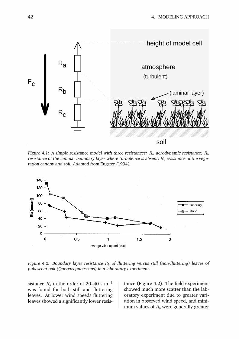
42 4. MODELING APPROACH
.
height of model cell
atmosphere
soil
Fc
Ra
Rb
Rc
(turbulent)
(laminar layer)
Figure 4.1: A simple resistance model with three resistances: Ra aerodynamic resistance; Rb
resistance of the laminar boundary layer where turbulence is absent; Rc resistance of the vege-tation canopy and soil. Adapted from Eugster (1994).
Figure 4.2: Boundary layer resistance Rb of fluttering versus still (non-fluttering) leaves ofpubescent oak (Quercus pubescens) in a laboratory experiment.
sistance Rb in the order of 20–40 s m−1
was found for both still and flutteringleaves. At lower wind speeds flutteringleaves showed a significantly lower resis-
tance (Figure 4.2). The field experimentshowed much more scatter than the lab-oratory experiment due to greater vari-ation in observed wind speed, and mini-mum values of Rb were generally greater

4.5 DEPOSITION MODULE 43
Table 4.1: Model parameters prescribed for various land use types in modeling canopy resis-tance Rc (in units of s m−1) for SO2 dry deposition.
land use season Rc,min Rc,max Rnight Rwet
urban built-up area spring 1000 1000 1000 1000summer 1000 1000 1000 0early fall 1000 1000 1000 1000late fall 1000 1000 1000 1000winter 200 200 200 200
agricultural crop spring 50 75 100 0summer 70 200 500 0early fall 500 500 500 100late fall 50 50 50 50winter 100 100 100 100
pasture land spring 100 200 400 0summer 100 200 500 0early fall 500 500 500 500late fall 500 500 500 500winter 100 100 100 100
deciduous forest spring 100 400 1000 0summer 60 300 1000 0early fall 1000 1000 1000 500late fall 1000 1000 1000 500winter 1000 1000 1000 1000
coniferous forest spring 150 400 1000 0summer 150 400 1000 0early fall 800 800 800 100late fall 800 1000 1000 100winter 500 500 500 500
riparian forest spring 100 400 1000 0summer 70 300 1000 0early fall 800 800 800 300late fall 800 800 1000 300winter 800 800 800 800
water surface all seasons 0 0 0 0
bog or wetland spring 50 75 100 0summer 50 75 100 0early fall 100 100 100 75late fall 100 100 100 75winter 100 100 100 100
mixed agricultural land spring 75 150 250 0summer 100 200 500 0early fall 500 500 500 100late fall 200 200 200 100winter 100 100 100 100
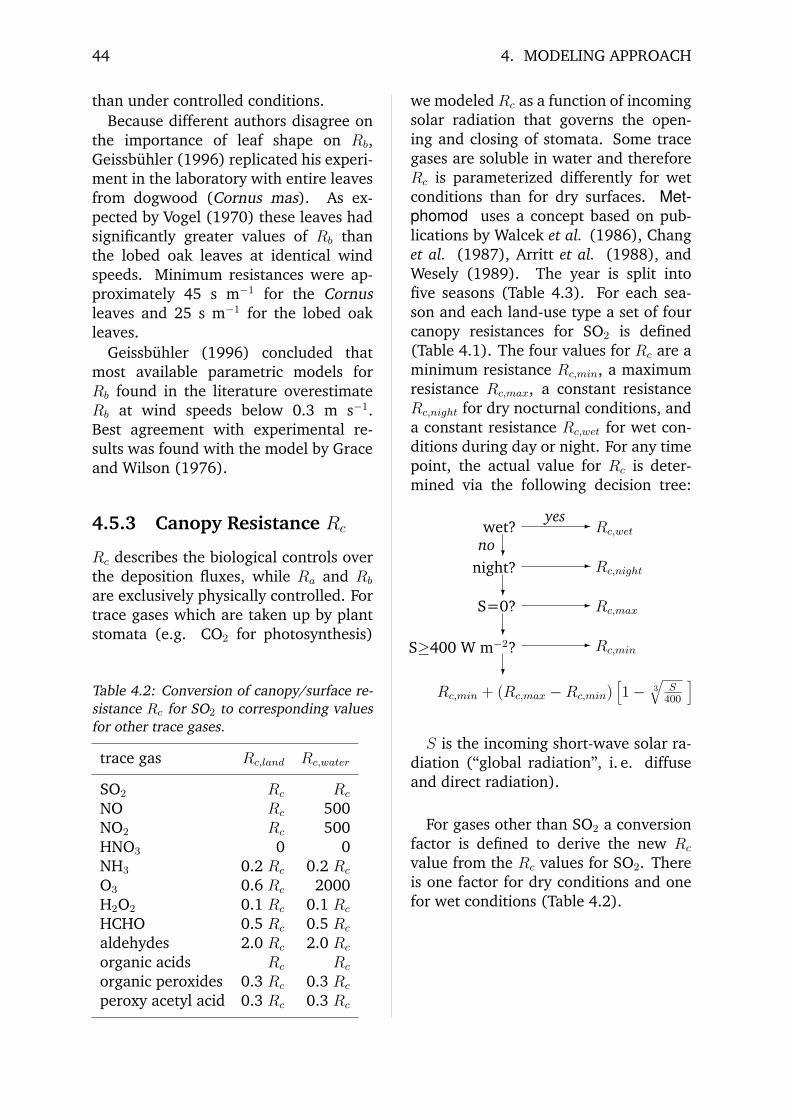
44 4. MODELING APPROACH
than under controlled conditions.Because different authors disagree on
the importance of leaf shape on Rb,Geissbuhler (1996) replicated his experi-ment in the laboratory with entire leavesfrom dogwood (Cornus mas). As ex-pected by Vogel (1970) these leaves hadsignificantly greater values of Rb thanthe lobed oak leaves at identical windspeeds. Minimum resistances were ap-proximately 45 s m−1 for the Cornusleaves and 25 s m−1 for the lobed oakleaves.
Geissbuhler (1996) concluded thatmost available parametric models forRb found in the literature overestimateRb at wind speeds below 0.3 m s−1.Best agreement with experimental re-sults was found with the model by Graceand Wilson (1976).
4.5.3 Canopy Resistance Rc
Rc describes the biological controls overthe deposition fluxes, while Ra and Rb
are exclusively physically controlled. Fortrace gases which are taken up by plantstomata (e.g. CO2 for photosynthesis)
Table 4.2: Conversion of canopy/surface re-sistance Rc for SO2 to corresponding valuesfor other trace gases.
trace gas Rc,land Rc,water
SO2 Rc Rc
NO Rc 500NO2 Rc 500HNO3 0 0NH3 0.2 Rc 0.2 Rc
O3 0.6 Rc 2000H2O2 0.1 Rc 0.1 Rc
HCHO 0.5 Rc 0.5 Rc
aldehydes 2.0 Rc 2.0 Rc
organic acids Rc Rc
organic peroxides 0.3 Rc 0.3 Rc
peroxy acetyl acid 0.3 Rc 0.3 Rc
we modeled Rc as a function of incomingsolar radiation that governs the open-ing and closing of stomata. Some tracegases are soluble in water and thereforeRc is parameterized differently for wetconditions than for dry surfaces. Met-phomod uses a concept based on pub-lications by Walcek et al. (1986), Changet al. (1987), Arritt et al. (1988), andWesely (1989). The year is split intofive seasons (Table 4.3). For each sea-son and each land-use type a set of fourcanopy resistances for SO2 is defined(Table 4.1). The four values for Rc are aminimum resistance Rc,min, a maximumresistance Rc,max, a constant resistanceRc,night for dry nocturnal conditions, anda constant resistance Rc,wet for wet con-ditions during day or night. For any timepoint, the actual value for Rc is deter-mined via the following decision tree:
wet?
night?
S=0?
S≥400 W m−2?
Rc,wet
Rc,night
Rc,max
Rc,min + (Rc,max −Rc,min)[1− 3
√S400
]Rc,min
yes
no-
-
-
-
?
?
?
?
S is the incoming short-wave solar ra-diation (“global radiation”, i. e. diffuseand direct radiation).
For gases other than SO2 a conversionfactor is defined to derive the new Rc
value from the Rc values for SO2. Thereis one factor for dry conditions and onefor wet conditions (Table 4.2).
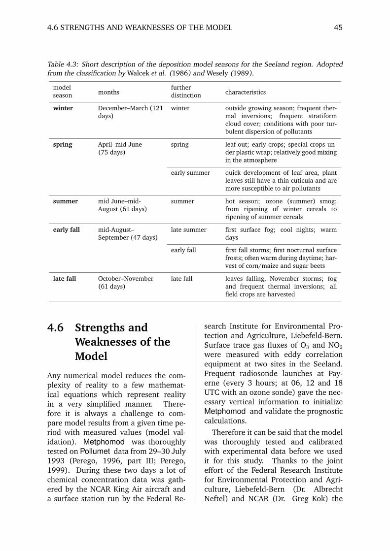
4.6 STRENGTHS AND WEAKNESSES OF THE MODEL 45
Table 4.3: Short description of the deposition model seasons for the Seeland region. Adoptedfrom the classification by Walcek et al. (1986) and Wesely (1989).
modelseason months
furtherdistinction characteristics
winter December–March (121days)
winter outside growing season; frequent ther-mal inversions; frequent stratiformcloud cover; conditions with poor tur-bulent dispersion of pollutants
spring April–mid-June(75 days)
spring leaf-out; early crops; special crops un-der plastic wrap; relatively good mixingin the atmosphere
early summer quick development of leaf area, plantleaves still have a thin cuticula and aremore susceptible to air pollutants
summer mid June–mid-August (61 days)
summer hot season; ozone (summer) smog;from ripening of winter cereals toripening of summer cereals
early fall mid-August–September (47 days)
late summer first surface fog; cool nights; warmdays
early fall first fall storms; first nocturnal surfacefrosts; often warm during daytime; har-vest of corn/maize and sugar beets
late fall October–November(61 days)
late fall leaves falling, November storms; fogand frequent thermal inversions; allfield crops are harvested
4.6 Strengths andWeaknesses of theModel
Any numerical model reduces the com-plexity of reality to a few mathemat-ical equations which represent realityin a very simplified manner. There-fore it is always a challenge to com-pare model results from a given time pe-riod with measured values (model val-idation). Metphomod was thoroughlytested on Pollumet data from 29–30 July1993 (Perego, 1996, part III; Perego,1999). During these two days a lot ofchemical concentration data was gath-ered by the NCAR King Air aircraft anda surface station run by the Federal Re-
search Institute for Environmental Pro-tection and Agriculture, Liebefeld-Bern.Surface trace gas fluxes of O3 and NO2
were measured with eddy correlationequipment at two sites in the Seeland.Frequent radiosonde launches at Pay-erne (every 3 hours; at 06, 12 and 18UTC with an ozone sonde) gave the nec-essary vertical information to initializeMetphomod and validate the prognosticcalculations.
Therefore it can be said that the modelwas thoroughly tested and calibratedwith experimental data before we usedit for this study. Thanks to the jointeffort of the Federal Research Institutefor Environmental Protection and Agri-culture, Liebefeld-Bern (Dr. AlbrechtNeftel) and NCAR (Dr. Greg Kok) the

46 4. MODELING APPROACH
concentrations of a large set of chemicaltrace gases were measured during thatperiod. However, of the 39 substancesincluded in Metphomod only a smallfraction were actually measured, makingit difficult to verify the model outputs forthe substances that were not measured.On the other hand, the comparison withavailable data from Pollumet 1993 is thebest that one can actually do in Switzer-land and probably also for most otherlocations in the world. This validationof Metphomod via the Pollumet data(Perego, 1999) is considered a strengthof the model.
Another model strength, is the directcoupling of air chemistry with the con-current meteorological processes in thelower troposphere. This improves theability of Metphomod to model thesmall-scale regional variation in nitrogendry deposition which is required for a re-gion with complex topography, such asthe Seeland and the adjacent Jura moun-tain ranges.
Not really weak points, but items thatshould be improved in the future, are(a) the heterogeneous chemistry, (b) thechemistry of NH3, (c) the biological con-trols over dry deposition, and (d) theundesirable decoupling of the depositionmodule from the energy balance modulein the model:
(a) At present, Metphomod modelshomogeneous gas-phase chemistryonly. Thus, no phase change of anysubstance is considered, i. e. build-ing of aerosol droplets and particlesdoes not occur in the model. Andfoggy or rainy events are not ade-quately modeled with Metphomod.
(b) NH3 does not belong to the setof photochemically reactive species.For the present study we added NH3
as a tracer that may react to NH+4
in the gas phase. However, in fur-ther studies it would be desirable to
define at least the reaction of NH3
with water droplets in the air. Atpresent we use a canopy resistancefor NH3 that is representative forgaseous NH+
4 as well. Therefore, theresults are labeled with NHx in Sec-tion 6 (NHx=NH3+NH+
4,(gaseous)).
(c) Biological control of dry deposi-tion is represented by the canopylayer resistance Rc only. This re-sistance varies according to solarshort-wave radiation (page 44) un-der dry conditions. There is nowater stress feedback in our cur-rent model. This means that drydeposition to plants may be over-estimated under drought conditionswhen plants close their stomata de-spite high solar radiation to preventthemselves from wilting.
(d) A key issue in a mesoscale modelis the treatment of surface energyfluxes. They determine the inter-action between the atmosphere andthe local surface and heavily influ-ence the air temperature and mois-ture in the model atmosphere. Al-though there is a close link betweenthese energy fluxes and plant activ-ity, the current version of Metpho-mod has no coupling between thetwo. Thus, the surface energy bal-ance may differ between the me-teorological part of the model andthe deposition module. This incon-sistency is widely spread in atmo-spheric modeling and attempts tostraighten out this problem in futuremodel generations were only startedrecently.
4.7 Concluding Remarks
Although we try to lay open the weak-nesses of our model approach it must be

4.7 CONCLUDING REMARKS 47
emphasized that Metphomod is an up-to-date mesoscale model and most issuesmentioned here are common to all cur-rent mesoscale models, not only to Met-phomod. We hope we were able to shedsome light on the black box “modeling”method for people not familiar with thiskind of approach. Understanding the as-sumptions on which a model is basedstrongly helps with the interpretation ofthe results.
5. Selection of Representative Daysand Model Inputs
5.1 Classification ofTurbulent TransportConditions
A new classification of turbulent trans-port conditions in the area of interest,the Seeland region with the adjacent up-lands of the Prealps in the south-east,and the Jura mountains in the north-west, was developed by Leuenberger(1996). Previously, Eugster (1994) hadshown that the relationship betweensurface fluxes of NO2 and the stan-dard synoptic weather classification af-ter Schuepp (1968) is not very wellsuited to regional dry deposition stud-ies and that a more detailed approachis needed. Before starting to developyet another classification scheme, Leuen-berger (1996) tested the performanceof weather classification schemes byHess and Brezowsky, (1969), Schuepp(1968), Wanner and Kunz (1977), Per-ret (1987), Rickli (1988), Wanner andFurger (1990), Furger (1990), andKunzle and Neu (1994). Despite the use-fulness of these approaches for the appli-cations for which they were designed for,none of them gave satisfactory results formesoscale trace gas flux modeling withMetphomod. Leuenberger (1996) statesthat the primary problems were scale is-sues (weather classifications tend to ad-dress scales of a whole continent ratherthan a specific region), problems withapplicability to a different locality otherthan the one for which they were devel-
oped for, and differences in key informa-tion that the classifications were able togive.
Thus, Leuenberger (1996) developeda classification that addresses the rele-vant information needed to select rep-resentative days for numerical modelingwith Metphomod. The most importantinformation that is required to character-ize a specific day in terms of turbulenttransport conditions for modeling tracegas fluxes are
• prevailing wind direction;
• typical wind speed (with or withoutthe knowledge of its diurnal cycle);
• thermal stability of the atmosphericboundary layer.
Eugster and Hesterberg (1996) foundthat daily total dry deposition of NO2
is dominated by the fluxes during themorning hours after the morning rushhour, while the afternoon and eveningconditions only contribute a minor frac-tion to the daily total deposition. There-fore, Leuenberger’s (1996) classificationprimarily aims at capturing daytime con-ditions, while nocturnal conditions haveonly a second priority in the classifica-tion scheme.
One requirement for the new classi-fication was to be as objective as pos-sible (allowing automatic classification),and that it be based on easily availabledata from the automatic weather sta-tion network ANETZ of the Swiss Mete-orological Office. Thus, no radiosonde
48

5.1 CLASSIFICATION OF TURBULENT TRANSPORT CONDITIONS 49
data was incorporated into the classi-fication. The vertical structure of theatmospheric boundary layer was deter-mined from vertical gradients betweentwo ANETZ stations at low elevationand three mountain top stations: Napf,1406 m a.s.l.; Chasseral, 1599 m a.s.l.;and Moleson, 1972 m a.s.l. (Figure 5.1).
The data used for the classificationwere the 10-minute average values fromthe years 1990 to 1993. Leuenberger(1996) suggested a six-step classificationscheme with the following steps:
1. Wind direction. For each of the fiveweather stations it is determinedwhether the wind direction is pri-marily from NE or from SW. The lim-its between these two sectors wereadjusted slightly for each station totake local channeling effects of thewind flow into account.
2. Initial number of transport condi-tions. From the results of step 1 aninitial class number was assigned toeach turbulent transport class. Withfive weather stations and two winddirection sectors this gives 25 = 32class numbers (0–31).
3. Thermal inversion criterion. Allcases where at least two out of thethree weather stations at the lowestelevations showed a thermal inver-sion (potential temperature at lowaltitude is colder than potential tem-perature at higher altitude) wereclassified separately into two inver-sion classes (Inv1 and Inv2).
4. Frequency of occurrence. Based onthe classification into classes 0–31,Inv1, and Inv2, the frequency of oc-currence during the four years ofdata (1990–1993) was determinedfor each class.
5. Significance test. Classes with a fre-quency of occurrence of more than
5% were further analyzed in the fol-lowing step.
6. Wind speed. The most commonclasses were split up into smallerclasses by wind speed. The classboundaries were defined individ-ually according to best availableknowledge on how differences inwind speed would lead to regionaldifferences in trace gas dry deposi-tion.
Based on this classification, referencedays were selected for modeling withMetphomod. The reference days wereselected in such a way that equal cover-age of the five seasons (Chapter 4.5.3;Table 4.3) was obtained, and that foreach season the most important turbu-lent transport conditions should be rep-resented. Originally we estimated tobe able to model approximately 15 ref-erence days with available funding andmanpower, three days for each of the fiveseasons.
The classification result by Leuen-berger (1996) for the study region is pre-sented in Table 5.1 for conditions withprevailing north-easterly winds, and inTable 5.2 for conditions with prevailingsouth-westerly flow. North-easterly flowis represented by eight classes whereofthree are dominated by a thermal inver-sion that traps air pollutants in a shal-low boundary layer over the Seelandregion. South-westerly flow is charac-terized by just four major classes, twoof them with a thermal inversion. Be-cause south-westerly flow is also associ-ated with the passage of weather frontsand thus with flushing of the polluted airin a large valley like the Seeland, we fur-ther split up the overwhelmingly dom-inant class 0 into various wind-speedclasses to take into account the differenteffects of fronts and ordinary weak-windconditions on trace gas fluxes and depo-sition in this region.

50 5. SELECTION OF REPRESENTATIVE DAYS AND MODEL INPUTS
Table 5.1: Classification of turbulent transport classes in the Seeland region during the years1990–1993. Classes with predominantly north-easterly flow. The flow type is characterizedby the prevailing wind direction at all 5 stations in Figure 5.1. An
⊗indicates that the wind
direction at this station does not influence the classification. Classes 16/7 and 31 are furtherseparated into subclasses according to the average wind speed u measured at station 1 (Pay-erne).
frequencyclass flow type (station 1-2-3-4-5)absolute relative
Inv1b NE-SW-⊗
-⊗
-⊗
89 11.3%Inv1d NE-NE-
⊗-⊗
-⊗
25 3.2%Inv2b NE-SW-
⊗-⊗
-⊗
50 6.4%1 NE-SW-SW-SW-SW 58 7.4%16/7 NE-NE-NE-SW-SW 217 27.6%—a u < 1.1 m s−1 71 9.0%—b 1.1 m s−1 ≤ u < 2.0 m s−1 97 12.3%—c u ≥ 2.0 m s−1 49 6.2%26 NE-NE-NE-NE-SW 53 6.7%27 NE-NE-NE-SW-NE 68 8.7%31 NE-NE-NE-NE-NE 153 19.5%—a u < 2.5 m s−1 21 2.7%—b 2.5 m s−1 ≤ u < 4.5 m s−1 68 8.7%—c u ≥ 4.5 m s−1 38 4.8%
total classified 713 90.7%grand total of NE classes 786 100.0%remaining classes 73 9.3%
Table 5.2: Same as Table 5.1 for the classes with predominantly south-westerly flow. Class 0 isfurther separated into subclasses according to the average wind speed u measured at station 1(Payerne).
frequencyclass flow type (station 1-2-3-4-5)absolute relative
Inv1a SW-SW-⊗
-⊗
-⊗
34 5.5%Inv2a SW-SW-
⊗-⊗
-⊗
30 4.9%0 SW-SW-SW-SW-SW 442 71.9%—a u < 1.5 m s−1 52 8.5%—b 1.5 m s−1 ≤ u < 4.0 m s−1 167 27.2%—c 4.0 m s−1 ≤ u < 6.0 m s−1 144 23.4%—d u ≥ 6.0 m s−1 79 12.8%3 SW-SW-NE-SW-SW 77 12.5%
total classified 583 94.8%grand total of SW classes 615 100.0%remaining classes 32 5.2%
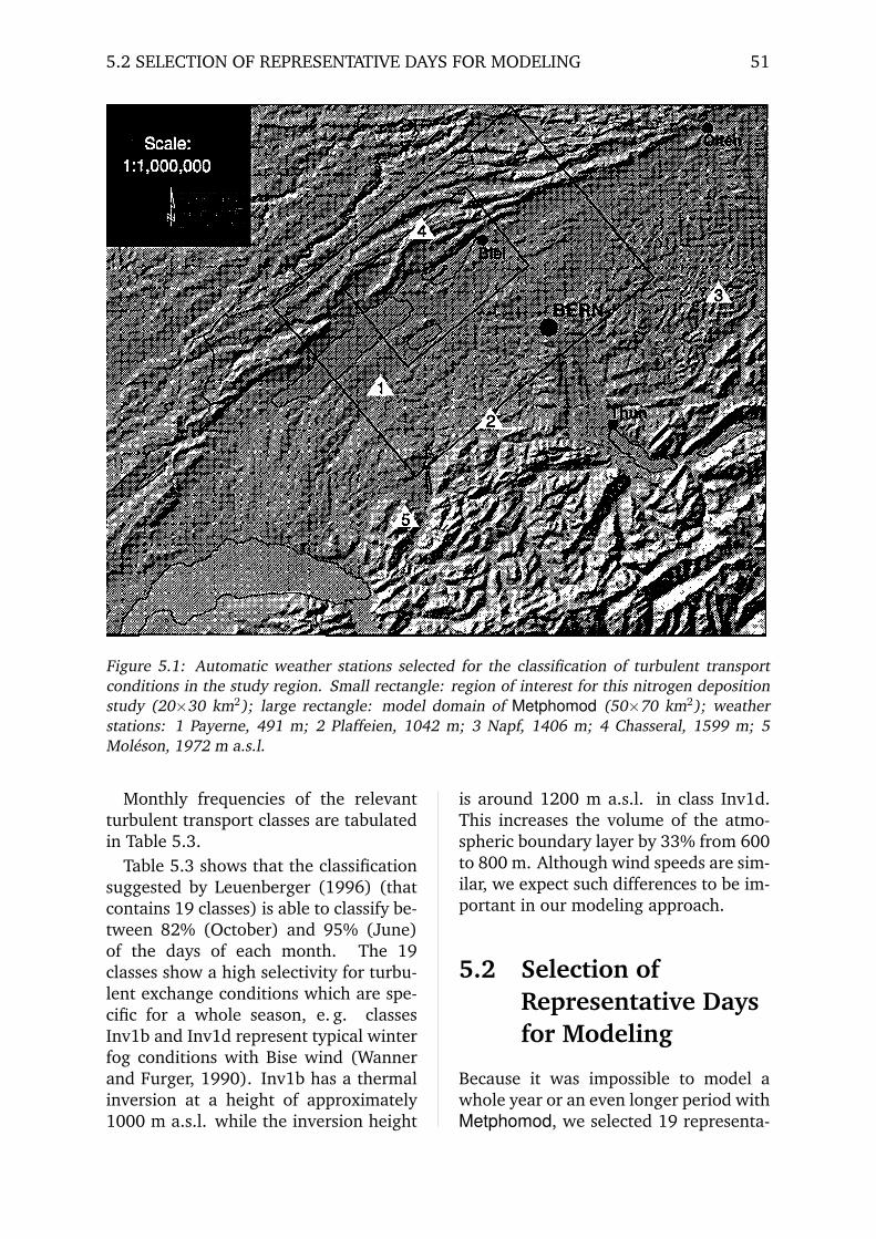
5.2 SELECTION OF REPRESENTATIVE DAYS FOR MODELING 51
Figure 5.1: Automatic weather stations selected for the classification of turbulent transportconditions in the study region. Small rectangle: region of interest for this nitrogen depositionstudy (20×30 km2); large rectangle: model domain of Metphomod (50×70 km2); weatherstations: 1 Payerne, 491 m; 2 Plaffeien, 1042 m; 3 Napf, 1406 m; 4 Chasseral, 1599 m; 5Moleson, 1972 m a.s.l.
Monthly frequencies of the relevantturbulent transport classes are tabulatedin Table 5.3.
Table 5.3 shows that the classificationsuggested by Leuenberger (1996) (thatcontains 19 classes) is able to classify be-tween 82% (October) and 95% (June)of the days of each month. The 19classes show a high selectivity for turbu-lent exchange conditions which are spe-cific for a whole season, e. g. classesInv1b and Inv1d represent typical winterfog conditions with Bise wind (Wannerand Furger, 1990). Inv1b has a thermalinversion at a height of approximately1000 m a.s.l. while the inversion height
is around 1200 m a.s.l. in class Inv1d.This increases the volume of the atmo-spheric boundary layer by 33% from 600to 800 m. Although wind speeds are sim-ilar, we expect such differences to be im-portant in our modeling approach.
5.2 Selection ofRepresentative Daysfor Modeling
Because it was impossible to model awhole year or an even longer period withMetphomod, we selected 19 representa-
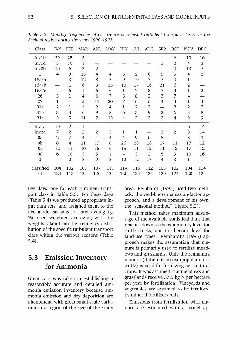
52 5. SELECTION OF REPRESENTATIVE DAYS AND MODEL INPUTS
Table 5.3: Monthly frequencies of occurrence of relevant turbulent transport classes in theSeeland region during the years 1990–1993.
Class JAN FEB MAR APR MAY JUN JUL AUG SEP OCT NOV DEC
Inv1b 29 25 3 — — — — — — 6 10 16Inv1d 5 10 1 — — — — — 1 2 4 2Inv2b 10 6 3 2 — — — — — 9 13 7
1 4 3 13 4 4 6 2 6 5 5 4 216/7a — 3 12 8 5 9 10 7 7 9 1 —16/7b — 1 6 3 15 10 17 16 21 6 2 —16/7c — 6 1 6 6 1 7 8 7 4 1 2
26 3 1 4 6 7 8 8 2 3 7 4 —27 1 — 5 11 20 7 6 6 4 3 1 431a 2 1 1 2 4 1 2 2 — 2 2 231b 3 3 6 9 8 6 5 9 2 6 3 831c 2 5 11 7 12 4 3 3 2 4 2 9
Inv1a 10 2 1 — — — — — — 1 6 14Inv2a 7 2 2 2 3 1 1 — 3 2 3 14
0a 2 7 4 1 4 4 9 6 8 1 3 30b 8 4 11 17 8 26 20 16 17 11 17 120c 12 11 10 15 6 15 11 12 11 12 17 120d 6 10 5 5 1 4 3 2 8 9 10 163 — 2 8 9 8 12 12 17 4 3 1 1
classified 104 102 107 107 111 114 116 112 103 102 104 114of 124 113 124 120 124 120 124 124 120 124 120 124
tive days, one for each turbulent trans-port class in Table 5.3. For these days(Table 5.4) we produced appropriate in-put data sets, and assigned them to thefive model seasons for later averaging.We used weighted averaging with theweights taken from the frequency distri-bution of the specific turbulent transportclass within the various seasons (Table5.4).
5.3 Emission Inventoryfor Ammonia
Great care was taken in establishing areasonably accurate and detailed am-monia emission inventory because am-monia emission and dry deposition arephenomena with great small-scale varia-tion in a region of the size of the study
area. Reinhardt (1995) used two meth-ods: the well-known emission-factor ap-proach, and a development of his own,the “seasonal method” (Figure 5.2).
This method takes maximum advan-tage of the available statistical data thatreaches down to the community level forcattle stocks, and the hectare level forland-use types. Reinhardt’s (1995) ap-proach makes the assumption that ma-nure is primarily used to fertilize mead-ows and grasslands. Only the remainingmanure (if there is an overpopulation ofcattle) is used for fertilizing agriculturalcrops. It was assumed that meadows andgrasslands receive 37.5 kg N per hectareper year by fertilization. Vineyards andvegetables are assumed to be fertilizedby mineral fertilizers only.
Emissions from fertilization with ma-nure are estimated with a model ap-
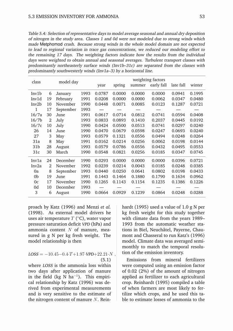
5.3 EMISSION INVENTORY FOR AMMONIA 53
Table 5.4: Selection of representative days to model average seasonal and annual dry depositionof nitrogen in the study area. Classes 1 and 0d were not modeled due to strong winds whichmade Metphomod crash. Because strong winds in the whole model domain are not expectedto lead to regional variation in trace gas concentrations, we reduced our modeling effort tothe remaining 17 days. The weighting factors indicate how the results from the individualdays were weighted to obtain annual and seasonal averages. Turbulent transport classes withpredominantly northeasterly surface winds (Inv1b–31c) are separated from the classes withpredominantly southwesterly winds (Inv1a–3) by a horizontal line.
weighting factorsclass model dayyear spring summer early fall late fall winter
Inv1b 6 January 1993 0.0787 0.0000 0.0000 0.0000 0.0941 0.1995Inv1d 19 February 1991 0.0208 0.0000 0.0000 0.0062 0.0347 0.0480Inv2b 10 November 1990 0.0448 0.0071 0.0085 0.0123 0.1287 0.0721
1 17 September 1993 — — — — — —16/7a 30 June 1991 0.0617 0.0714 0.0812 0.0741 0.0594 0.040816/7b 2 July 1993 0.0833 0.0893 0.1410 0.2037 0.0445 0.019216/7c 10 July 1990 0.0424 0.0500 0.0513 0.0741 0.0297 0.0240
26 14 June 1990 0.0470 0.0679 0.0598 0.0247 0.0693 0.024027 3 May 1993 0.0579 0.1321 0.0556 0.0494 0.0248 0.026431a 8 May 1991 0.0162 0.0214 0.0256 0.0062 0.0198 0.014431b 28 August 1993 0.0579 0.0786 0.0556 0.0432 0.0495 0.055331c 30 March 1990 0.0548 0.0821 0.0256 0.0185 0.0347 0.0745
Inv1a 24 December 1990 0.0293 0.0000 0.0000 0.0000 0.0396 0.0721Inv2a 2 November 1992 0.0239 0.0214 0.0043 0.0185 0.0248 0.0385
0a 8 September 1993 0.0440 0.0250 0.0641 0.0802 0.0198 0.04330b 19 June 1991 0.1443 0.1464 0.1880 0.1790 0.1634 0.09620c 17 November 1990 0.1265 0.1143 0.1154 0.1235 0.1386 0.12260d 10 December 1993 — — — — — —3 6 August 1990 0.0664 0.0929 0.1239 0.0864 0.0248 0.0288
proach by Katz (1996) and Menzi et al.(1998). As external model drivers heuses air temperature T (◦C), water vaporpressure saturation deficit VPD (hPa) andammonia content N of manure, mea-sured in g N per kg fresh weight. Themodel relationship is then
LOSS = −10.45−0.4·T+1.97·VPD+22.21·N ,(5.1)
where LOSS is the ammonia loss withintwo days after application of manurein the field (kg N ha−1). This empiri-cal relationship by Katz (1996) was de-rived from experimental measurementsand is very sensitive to the estimate ofthe nitrogen content of manure N . Rein-
hardt (1995) used a value of 1.0 g N perkg fresh weight for this study togetherwith climate data from the years 1989–1993 from the automatic weather sta-tions in Biel, Neuchatel, Payerne, Chau-mont and Chasseral to run Katz’s (1996)model. Climate data was averaged semi-monthly to match the temporal resolu-tion of the emission inventory.
Emissions from mineral fertilizerswere computed using an emission factorof 0.02 (2%) of the amount of nitrogenapplied as fertilizer to each agriculturalcrop. Reinhardt (1995) compiled a tableof when farmers are most likely to fer-tilize which crops, and he used this ta-ble to estimate losses of ammonia to the
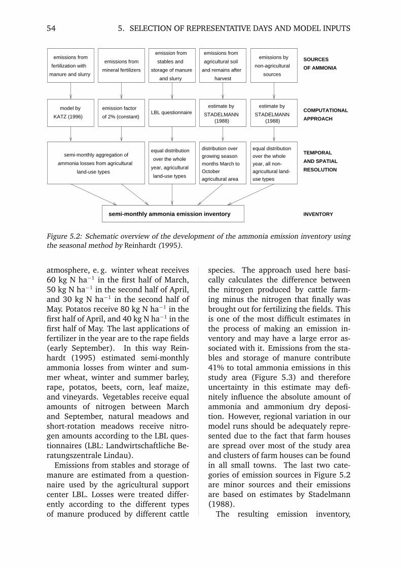
54 5. SELECTION OF REPRESENTATIVE DAYS AND MODEL INPUTS
growing season
months March to
October
agricultural area
over the whole
year, all non-
agricultural land-
use types
fertilization withmineral fertilizers
harvest
and remains after
agricultural soil
sources
non-agricultural
of 2% (constant)LBL questionnaire
(1988)STADELMANN
(1988)STADELMANN
land-use typesland-use types
year, agricultural
over the whole
SOURCES
COMPUTATIONAL
APPROACH
RESOLUTION
AND SPATIAL
TEMPORAL
INVENTORY
OF AMMONIAstables and
and slurry
emission from
emissions fromemissions from
emissions fromemissions by
model by emission factor estimate by estimate by
equal distribution distribution over equal distribution
manure and slurry
KATZ (1996)
storage of manure
semi-monthly ammonia emission inventory
semi-monthly aggregation of
ammonia losses from agricultural
Figure 5.2: Schematic overview of the development of the ammonia emission inventory usingthe seasonal method by Reinhardt (1995).
atmosphere, e. g. winter wheat receives60 kg N ha−1 in the first half of March,50 kg N ha−1 in the second half of April,and 30 kg N ha−1 in the second half ofMay. Potatos receive 80 kg N ha−1 in thefirst half of April, and 40 kg N ha−1 in thefirst half of May. The last applications offertilizer in the year are to the rape fields(early September). In this way Rein-hardt (1995) estimated semi-monthlyammonia losses from winter and sum-mer wheat, winter and summer barley,rape, potatos, beets, corn, leaf maize,and vineyards. Vegetables receive equalamounts of nitrogen between Marchand September, natural meadows andshort-rotation meadows receive nitro-gen amounts according to the LBL ques-tionnaires (LBL: Landwirtschaftliche Be-ratungszentrale Lindau).
Emissions from stables and storage ofmanure are estimated from a question-naire used by the agricultural supportcenter LBL. Losses were treated differ-ently according to the different typesof manure produced by different cattle
species. The approach used here basi-cally calculates the difference betweenthe nitrogen produced by cattle farm-ing minus the nitrogen that finally wasbrought out for fertilizing the fields. Thisis one of the most difficult estimates inthe process of making an emission in-ventory and may have a large error as-sociated with it. Emissions from the sta-bles and storage of manure contribute41% to total ammonia emissions in thisstudy area (Figure 5.3) and thereforeuncertainty in this estimate may defi-nitely influence the absolute amount ofammonia and ammonium dry deposi-tion. However, regional variation in ourmodel runs should be adequately repre-sented due to the fact that farm housesare spread over most of the study areaand clusters of farm houses can be foundin all small towns. The last two cate-gories of emission sources in Figure 5.2are minor sources and their emissionsare based on estimates by Stadelmann(1988).
The resulting emission inventory,
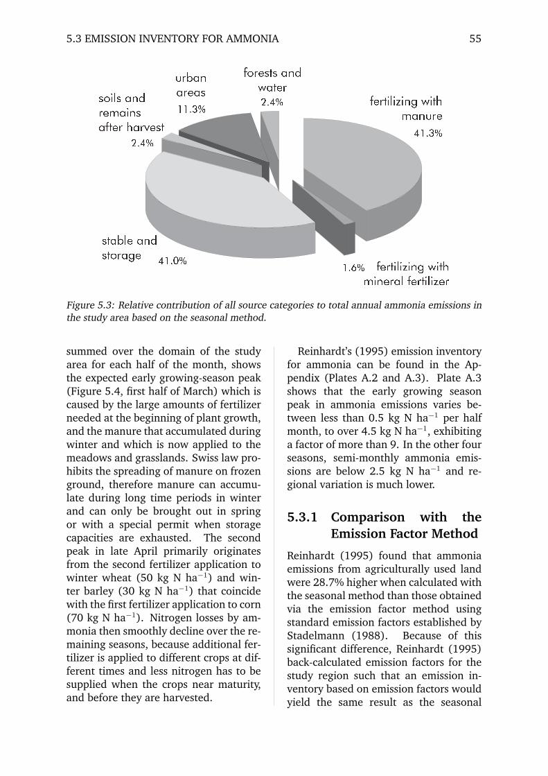
5.3 EMISSION INVENTORY FOR AMMONIA 55
fertilizing withmanure
fertilizing withmineral fertilizer
stable andstorage
soils andremainsafter harvest
urbanareas
forests andwater
41.3%
1.6%41.0%
2.4%
11.3% 2.4%
Figure 5.3: Relative contribution of all source categories to total annual ammonia emissions inthe study area based on the seasonal method.
summed over the domain of the studyarea for each half of the month, showsthe expected early growing-season peak(Figure 5.4, first half of March) which iscaused by the large amounts of fertilizerneeded at the beginning of plant growth,and the manure that accumulated duringwinter and which is now applied to themeadows and grasslands. Swiss law pro-hibits the spreading of manure on frozenground, therefore manure can accumu-late during long time periods in winterand can only be brought out in springor with a special permit when storagecapacities are exhausted. The secondpeak in late April primarily originatesfrom the second fertilizer application towinter wheat (50 kg N ha−1) and win-ter barley (30 kg N ha−1) that coincidewith the first fertilizer application to corn(70 kg N ha−1). Nitrogen losses by am-monia then smoothly decline over the re-maining seasons, because additional fer-tilizer is applied to different crops at dif-ferent times and less nitrogen has to besupplied when the crops near maturity,and before they are harvested.
Reinhardt’s (1995) emission inventoryfor ammonia can be found in the Ap-pendix (Plates A.2 and A.3). Plate A.3shows that the early growing seasonpeak in ammonia emissions varies be-tween less than 0.5 kg N ha−1 per halfmonth, to over 4.5 kg N ha−1, exhibitinga factor of more than 9. In the other fourseasons, semi-monthly ammonia emis-sions are below 2.5 kg N ha−1 and re-gional variation is much lower.
5.3.1 Comparison with theEmission Factor Method
Reinhardt (1995) found that ammoniaemissions from agriculturally used landwere 28.7% higher when calculated withthe seasonal method than those obtainedvia the emission factor method usingstandard emission factors established byStadelmann (1988). Because of thissignificant difference, Reinhardt (1995)back-calculated emission factors for thestudy region such that an emission in-ventory based on emission factors wouldyield the same result as the seasonal

56 5. SELECTION OF REPRESENTATIVE DAYS AND MODEL INPUTS
Jan
AJa
n B
Feb
AF
eb B
Mar
AM
ar B
Apr
AA
pr B
May
AM
ay B
Jun
AJu
n B
Jul A
Jul B
Aug
AA
ug B
Sep
AS
ep B
Oct
AO
ct B
Nov
AN
ov B
Dec
AD
ec B
0
20000
40000
60000
80000
100000
120000
140000kg
N p
er 1 / 2
mon
th
Figure 5.4: Semi-monthly ammonia emission totals for the study area. First half of monthlabeled A, second half labeled B.
method (Table 5.5).
Emission estimates from urban ar-eas, forest and water surfaces were ob-tained via the standard emission factortechnique, and thus did not differ inthe two approaches used by Reinhardt(1995). Including these source cat-egories, ammonia emissions estimatedwith the seasonal method were 23.8%higher in the domain of interest (28.7%if only agricultural land is considered)than the estimate with the old emissionfactors. Because Reinhardt’s (1995) sea-sonal method is based on more detailedinformation than the emission factormethod, we used the seasonal methodto produce the ammonia emission inven-tory for our model simulations. Emis-sion factors (Table 5.5) are only givenfor reference and for use in future stud-ies where the more data demanding sea-sonal method is not applicable.
The annual emission totals of bothmethods and the respective regionalvariation can be seen on color plate Fig-ure A.2, and the seasonal differencesfor the study region is displayed in Fig-
ure A.3. Because the length of a sea-son varies within our definition (Table4.3) we show semi-monthly total ammo-nia emissions in Plate A.3 to allow directcomparison between the individual pan-els.
Table 5.5: New and old emission factors (EF)(kg NH3-N ha−1 yr−1) for cattle in the studyarea, total population and relative contribu-tion to total ammonia emissions.
cattle total relative EFspecies number contrib. old new
cow 47261 87.4% 17.5 22.8pig 24615 4.4% 1.7 2.2horse 2509 2.4% 9.1 11.8sheepgoat
5996 1.4% 2.2 2.9
chicken 197548 4.4% 0.21 0.28
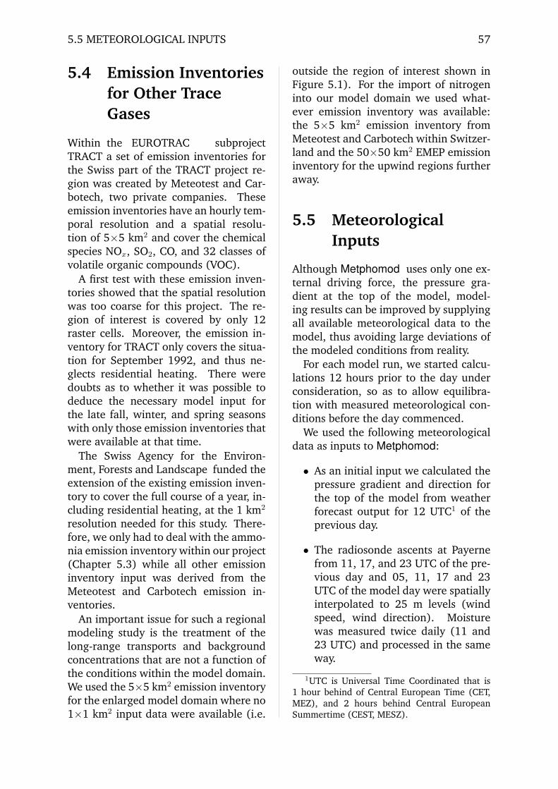
5.5 METEOROLOGICAL INPUTS 57
5.4 Emission Inventoriesfor Other TraceGases
Within the EUROTRAC subprojectTRACT a set of emission inventories forthe Swiss part of the TRACT project re-gion was created by Meteotest and Car-botech, two private companies. Theseemission inventories have an hourly tem-poral resolution and a spatial resolu-tion of 5×5 km2 and cover the chemicalspecies NOx, SO2, CO, and 32 classes ofvolatile organic compounds (VOC).
A first test with these emission inven-tories showed that the spatial resolutionwas too coarse for this project. The re-gion of interest is covered by only 12raster cells. Moreover, the emission in-ventory for TRACT only covers the situa-tion for September 1992, and thus ne-glects residential heating. There weredoubts as to whether it was possible todeduce the necessary model input forthe late fall, winter, and spring seasonswith only those emission inventories thatwere available at that time.
The Swiss Agency for the Environ-ment, Forests and Landscape funded theextension of the existing emission inven-tory to cover the full course of a year, in-cluding residential heating, at the 1 km2
resolution needed for this study. There-fore, we only had to deal with the ammo-nia emission inventory within our project(Chapter 5.3) while all other emissioninventory input was derived from theMeteotest and Carbotech emission in-ventories.
An important issue for such a regionalmodeling study is the treatment of thelong-range transports and backgroundconcentrations that are not a function ofthe conditions within the model domain.We used the 5×5 km2 emission inventoryfor the enlarged model domain where no1×1 km2 input data were available (i.e.
outside the region of interest shown inFigure 5.1). For the import of nitrogeninto our model domain we used what-ever emission inventory was available:the 5×5 km2 emission inventory fromMeteotest and Carbotech within Switzer-land and the 50×50 km2 EMEP emissioninventory for the upwind regions furtheraway.
5.5 MeteorologicalInputs
Although Metphomod uses only one ex-ternal driving force, the pressure gra-dient at the top of the model, model-ing results can be improved by supplyingall available meteorological data to themodel, thus avoiding large deviations ofthe modeled conditions from reality.
For each model run, we started calcu-lations 12 hours prior to the day underconsideration, so as to allow equilibra-tion with measured meteorological con-ditions before the day commenced.
We used the following meteorologicaldata as inputs to Metphomod:
• As an initial input we calculated thepressure gradient and direction forthe top of the model from weatherforecast output for 12 UTC1 of theprevious day.
• The radiosonde ascents at Payernefrom 11, 17, and 23 UTC of the pre-vious day and 05, 11, 17 and 23UTC of the model day were spatiallyinterpolated to 25 m levels (windspeed, wind direction). Moisturewas measured twice daily (11 and23 UTC) and processed in the sameway.
1UTC is Universal Time Coordinated that is1 hour behind of Central European Time (CET,MEZ), and 2 hours behind Central EuropeanSummertime (CEST, MESZ).
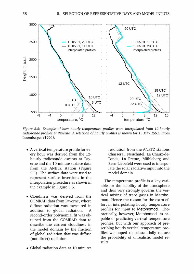
58 5. SELECTION OF REPRESENTATIVE DAYS AND MODEL INPUTS
-8 -4 0 4 8 12temperature,
oC
500
1000
1500
2000
2500
3000he
ight
, m a
.s.l.
12.05.91, 23 UTC13.05.91, 11 UTCinterpolated profiles
-4 0 4 8 12 16temperature,
oC
13.05.91, 11 UTC13.05.91, 23 UTCinterpolated profiles
0 UTC
1 UTC9 UTC
10 UTC
22 UTC
20 UTC12 UTC
15 UTC
12 UTC
20 UTC
Figure 5.5: Example of how hourly temperature profiles were interpolated from 12-hourlyradiosonde profiles at Payerne. A selection of hourly profiles is shown for 13 May 1991. FromLeuenberger (1996).
• A vertical temperature profile for ev-ery hour was derived from the 12-hourly radiosonde ascents at Pay-erne and the 10-minute surface datafrom the ANETZ station (Figure5.5). The surface data were used torepresent surface inversions in theinterpolation procedure as shown inthe example in Figure 5.5.
• Cloudiness was derived from theCOMRAD data from Payerne, wherediffuse radiation was measured inaddition to global radiation. Asecond-order polynomial fit was ob-tained from the COMRAD data todescribe the current cloudiness inthe model domain by the fractionof global radiation that was diffuse(not direct) radiation.
• Global radiation data at 10 minutes
resolution from the ANETZ stationsChasseral, Neuchatel, La Chaux-de-Fonds, La Fretaz, Muhleberg andBern-Liebefeld were used to interpo-late the solar radiative input into themodel domain.
The temperature profile is a key vari-able for the stability of the atmosphereand thus very strongly governs the ver-tical mixing of trace gases in Metpho-mod. Hence the reason for the extra ef-fort in interpolating hourly temperatureprofiles for input to Metphomod. The-oretically, however, Metphomod is ca-pable of predicting vertical temperatureprofiles, but with our approach of pre-scribing hourly vertical temperature pro-files we hoped to substantially reducethe probability of unrealistic model re-sults.
6. Dry Deposition of Nitrogen
6.1 Introduction
In this chapter we present the resultsof the Metphomod model runs. Colorplates can be found in Appendix A. Theresults for other forms of nitrogen depo-sition, essentially wet deposition (Chap-ter 7) and aerosol dry deposition (Chap-ter 8) will follow in subsequent chapters.
Seasonal and regional variation innitrogen dry deposition depends verymuch on atmospheric conditions andlength of season. Although there is aclear peak in ammonia emissions in thespring when all agricultural crops needa first application of fertilizer, manureor slurry (Figure 5.4 and Plate A.3),the resulting nitrogen dry deposition isnot only an important issue during thespring season.
In Section 6.2 we shall look at theseasonal and regional patterns for thenitrogen-containing species included inthe chemistry module of Metphomod. InSection 6.3 we shall look at the regionalvariation of total nitrogen dry depositionfor the individual days we modeled withMetphomod. This will reveal the influ-ence of atmospheric conditions on theregional variation of dry deposition.
The model output from Metphomod ispresented with an overlying layer show-ing the major rivers, lake shores, citiesand towns, and the topography withdashed contour lines (Figure 6.1). Forcomputational reasons the model do-main is not aligned with geographicNorth, but was rotated clockwise by anangle of 40◦. Thus, the apparent west–east extent of the Jura mountains and
the lakes of Neuchatel and Biel is ac-tually in the southwest–northeast direc-tion.
6.2 Seasonal andRegional Variation
The seasonal variation in dry depositionof total nitrogen, oxidized and reducedforms of nitrogen is shown in Figures6.2, 6.3, 6.5, 6.6, 6.8, and 6.9. Foreach of the three pairs of graphs we firstshow deposition totals per season (Fig-ures 6.2, 6.5 and 6.8) and then the samevalues converted to per-day depositionvalues (Figures 6.3, 6.6 and 6.9). Theseasonal totals are given for five subre-gions or surface types defined in Figure6.4, hereafter referred to as regions: (1)the agricultural areas of the Seeland ru-ral plain; (2) the meso- to xerothermicsouth slope of the Jura at elevations be-tween 429 and 1033 m a.s.l. (both for-est and grassland ecosystems occur inthis region); (3) the three lakes: Lakeof Neuchatel, Lake of Biel and Lake ofMurten; (4) a rectangular area encom-passing the urban area of Bern whichalso includes some adjacent semi-urbanareas; (5) forested hills at elevations be-tween 440 and 571 m a.s.l. in the See-land.
Because season lengths vary in theirnumber of days, we expect a larger sea-sonal dry deposition total from a longseason such as the winter season com-pared to a short season like early fall. Al-though different season lengths are rea-sonable and primarily reflect prevailing
59

60 6. DRY DEPOSITION OF NITROGEN
Figure 6.1: Topography (dashed lines), rivers and lake shores (bold lines), and local namesused in all following figures with model results, and in the color plates on pages 115–122. Thecontour line interval is 200 m from 500–1100 m a.s.l. and 100 m from 1100–1500 m a.s.l.Highest elevation is Mount Chasseral with 1606 m.
meteorological conditions, the nitrogendeposition per day is also of interest, al-though a large dry deposition during avery short time would not have a verylarge impact on annual dry depositiontotals. In this section we address the sea-sonal variations within the five regionsspecified above, and in Section 6.3 wewill look at the regional variations in thesame five regions for the 17 turbulenttransport classes used in this model ap-proach.
6.2.1 Total Nitrogen Deposi-tion
As expected the longest season (winter,121 days) also gets the highest input oftotal nitrogen (Figure 6.2). However, ifwe look at the deposition amounts per
day the seasonal variation is only small(Figure 6.3) compared with the differ-ences between the five regions. Thelakes receive by far the highest nitrogenloads, directly followed by the urban ar-eas.
In Figure 6.3 only the lakes and the ur-ban area of Bern show a clear seasonal-ity. The lakes get most nitrogen in winterand spring, while the urban area of Bernshows a winter maximum and a springminimum. The explanation for this isthe dominance of NHx deposition in to-tal nitrogen inputs to the lakes (comparealso Plates A.5 and A.7 in the Appendix),while nitrogen deposition in the urbanarea of Bern is also heavily influenced byNOy deposition.
Because most of the study area is non-urban and thus dominated by NHx inputs
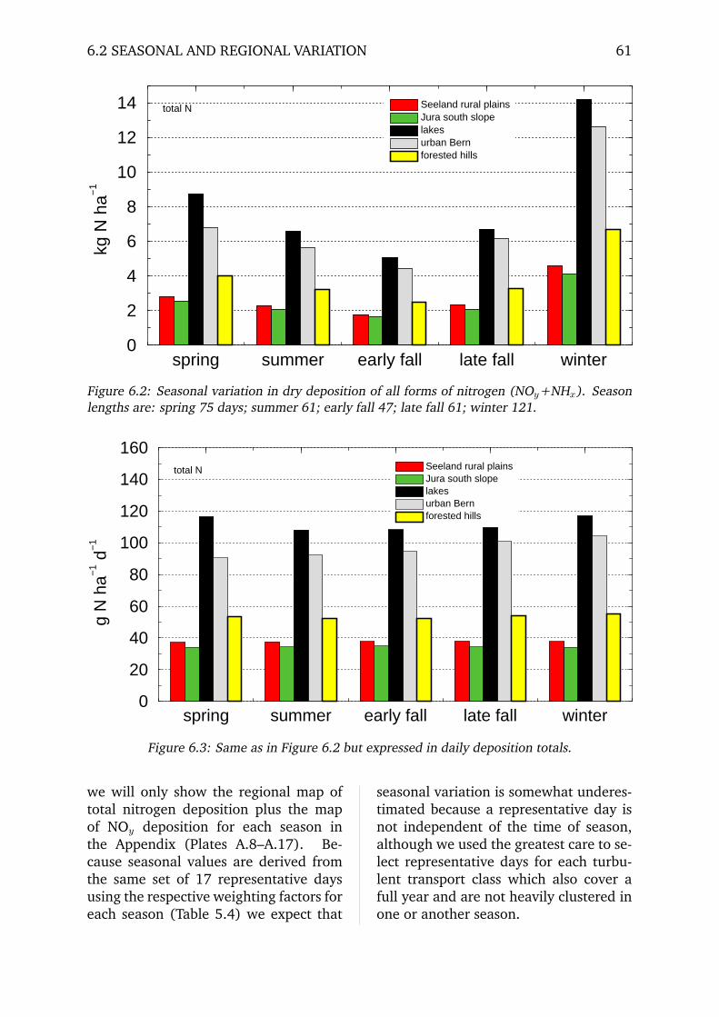
6.2 SEASONAL AND REGIONAL VARIATION 61
spring summer early fall late fall winter0
2
4
6
8
10
12
14kg
N h
a−1
Seeland rural plainsJura south slopelakesurban Bernforested hills
total N
Figure 6.2: Seasonal variation in dry deposition of all forms of nitrogen (NOy+NHx). Seasonlengths are: spring 75 days; summer 61; early fall 47; late fall 61; winter 121.
spring summer early fall late fall winter0
20
40
60
80
100
120
140
160
g N
ha−
1 d−
1
Seeland rural plainsJura south slopelakesurban Bernforested hills
total N
Figure 6.3: Same as in Figure 6.2 but expressed in daily deposition totals.
we will only show the regional map oftotal nitrogen deposition plus the mapof NOy deposition for each season inthe Appendix (Plates A.8–A.17). Be-cause seasonal values are derived fromthe same set of 17 representative daysusing the respective weighting factors foreach season (Table 5.4) we expect that
seasonal variation is somewhat underes-timated because a representative day isnot independent of the time of season,although we used the greatest care to se-lect representative days for each turbu-lent transport class which also cover afull year and are not heavily clustered inone or another season.

62 6. DRY DEPOSITION OF NITROGEN
������������������������
������������������������
���������������������������������������������������������������������������������������������������
���������������������������������������������������������������������������������������������������
������������������������������������������
������������������������������������������
������������������������������
������������������������������
���������������
���������������
Figure 6.4: Areas selected for regional averaging. Horizontal lines: Seeland rural plains; black:Jura south slope; inclined shade: lakes; vertical lines: urban area including Bern; gray: forestedhills (Jolimont, Schaltenrain, Bargenholz). Underlaying topography is grayshaded according tothe scale at right (elevations in m a.s.l.).
6.2.2 Deposition of OxidizedNitrogen
Deposition of oxidized nitrogen is thedominant form of nitrogen dry deposi-tion along major traffic axes and in citycenters. This is not a new finding andtherefore the extent of the region se-lected for describing urban Bern (Figure6.4) also includes suburban areas, cityforests and adjacent agricultural areas,a total of 60 km2, of which only a frac-tion is heavily polluted by NOx emittingsources. In this landscape mixture wefound that 48% of the total nitrogen drydeposition input of 35.6 kg N ha−1 yr−1
is in the form of oxidized nitrogen(17.2 kg N ha−1 yr−1) and 52% is in re-duced form (18.4 kg N ha−1 yr−1). Thuswe still found a slightly dominant NHx
deposition even in this area. This canbe explained by the different uptake re-sistances for oxidized and reduced formsof nitrogen. Because oxidized nitrogencompounds are not as well soluble inwater as NH3, the uptake resistance forNOy compounds is generally higher thanfor NH3 (Rc is held constant in Metpho-mod over urban areas at a value of 1000and 200 s m−1 for NOy and NH3, re-spectively; see Tables 4.1 and 4.2). Thisleads to the situation where NOy com-ponents are transported over longer dis-tances than NHx. Thus, NOx dry de-position dominates only in areas whereNOx emissions (and concentrations) aremanytimes higher than NH3 values. Thisis typically only the case in the center ofcities and large towns, within a few 100m of important traffic axes, and in some

6.2 SEASONAL AND REGIONAL VARIATION 63
spring summer early fall late fall winter0
1
2
3
4
5
6
7kg
N h
a−1
Seeland rural plainsJura south slopelakesurban Bernforested hills
NOy
Figure 6.5: Seasonal variation in dry deposition of oxidized forms of nitrogen(NOy=NO+NO2+NO3+HNO3). Season lengths are: spring 75 days; summer 61; early fall47; late fall 61; winter 121.
spring summer early fall late fall winter0
20
40
60
80
g N
ha−
1 d−
1
Seeland rural plainsJura south slopelakesurban Bernforested hills
NOy
Figure 6.6: Same as in Figure 6.5 but expressed in daily deposition totals.
industrial areas.The color plates in the Appendix
clearly show the high spatial variation ofNOy deposition during all seasons withinthe 60 km2 that were averaged for theurban area of Bern. Figure 6.7 shows
the ratio between dry deposition of ox-idized forms of nitrogen versus dry de-position of reduced forms of nitrogenfor the whole year at full spatial resolu-tion. In this figure we plotted the 1:1line as a solid line separating the ar-
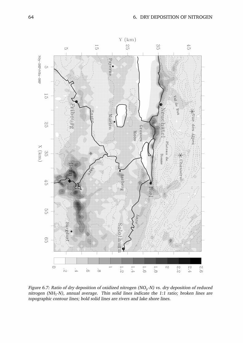
64 6. DRY DEPOSITION OF NITROGEN
Figure 6.7: Ratio of dry deposition of oxidized nitrogen (NOy-N) vs. dry deposition of reducednitrogen (NH3-N), annual average. Thin solid lines indicate the 1:1 ratio; broken lines aretopographic contour lines; bold solid lines are rivers and lake shore lines.
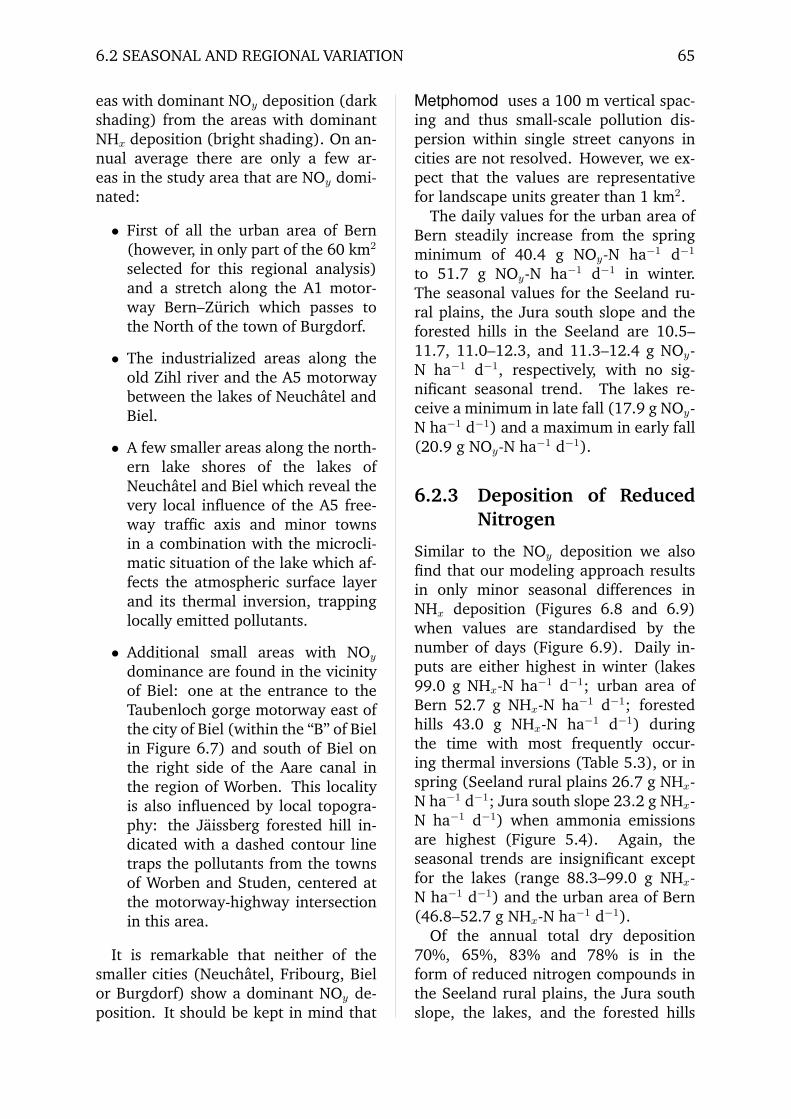
6.2 SEASONAL AND REGIONAL VARIATION 65
eas with dominant NOy deposition (darkshading) from the areas with dominantNHx deposition (bright shading). On an-nual average there are only a few ar-eas in the study area that are NOy domi-nated:
• First of all the urban area of Bern(however, in only part of the 60 km2
selected for this regional analysis)and a stretch along the A1 motor-way Bern–Zurich which passes tothe North of the town of Burgdorf.
• The industrialized areas along theold Zihl river and the A5 motorwaybetween the lakes of Neuchatel andBiel.
• A few smaller areas along the north-ern lake shores of the lakes ofNeuchatel and Biel which reveal thevery local influence of the A5 free-way traffic axis and minor townsin a combination with the microcli-matic situation of the lake which af-fects the atmospheric surface layerand its thermal inversion, trappinglocally emitted pollutants.
• Additional small areas with NOy
dominance are found in the vicinityof Biel: one at the entrance to theTaubenloch gorge motorway east ofthe city of Biel (within the “B” of Bielin Figure 6.7) and south of Biel onthe right side of the Aare canal inthe region of Worben. This localityis also influenced by local topogra-phy: the Jaissberg forested hill in-dicated with a dashed contour linetraps the pollutants from the townsof Worben and Studen, centered atthe motorway-highway intersectionin this area.
It is remarkable that neither of thesmaller cities (Neuchatel, Fribourg, Bielor Burgdorf) show a dominant NOy de-position. It should be kept in mind that
Metphomod uses a 100 m vertical spac-ing and thus small-scale pollution dis-persion within single street canyons incities are not resolved. However, we ex-pect that the values are representativefor landscape units greater than 1 km2.
The daily values for the urban area ofBern steadily increase from the springminimum of 40.4 g NOy-N ha−1 d−1
to 51.7 g NOy-N ha−1 d−1 in winter.The seasonal values for the Seeland ru-ral plains, the Jura south slope and theforested hills in the Seeland are 10.5–11.7, 11.0–12.3, and 11.3–12.4 g NOy-N ha−1 d−1, respectively, with no sig-nificant seasonal trend. The lakes re-ceive a minimum in late fall (17.9 g NOy-N ha−1 d−1) and a maximum in early fall(20.9 g NOy-N ha−1 d−1).
6.2.3 Deposition of ReducedNitrogen
Similar to the NOy deposition we alsofind that our modeling approach resultsin only minor seasonal differences inNHx deposition (Figures 6.8 and 6.9)when values are standardised by thenumber of days (Figure 6.9). Daily in-puts are either highest in winter (lakes99.0 g NHx-N ha−1 d−1; urban area ofBern 52.7 g NHx-N ha−1 d−1; forestedhills 43.0 g NHx-N ha−1 d−1) duringthe time with most frequently occur-ing thermal inversions (Table 5.3), or inspring (Seeland rural plains 26.7 g NHx-N ha−1 d−1; Jura south slope 23.2 g NHx-N ha−1 d−1) when ammonia emissionsare highest (Figure 5.4). Again, theseasonal trends are insignificant exceptfor the lakes (range 88.3–99.0 g NHx-N ha−1 d−1) and the urban area of Bern(46.8–52.7 g NHx-N ha−1 d−1).
Of the annual total dry deposition70%, 65%, 83% and 78% is in theform of reduced nitrogen compounds inthe Seeland rural plains, the Jura southslope, the lakes, and the forested hills
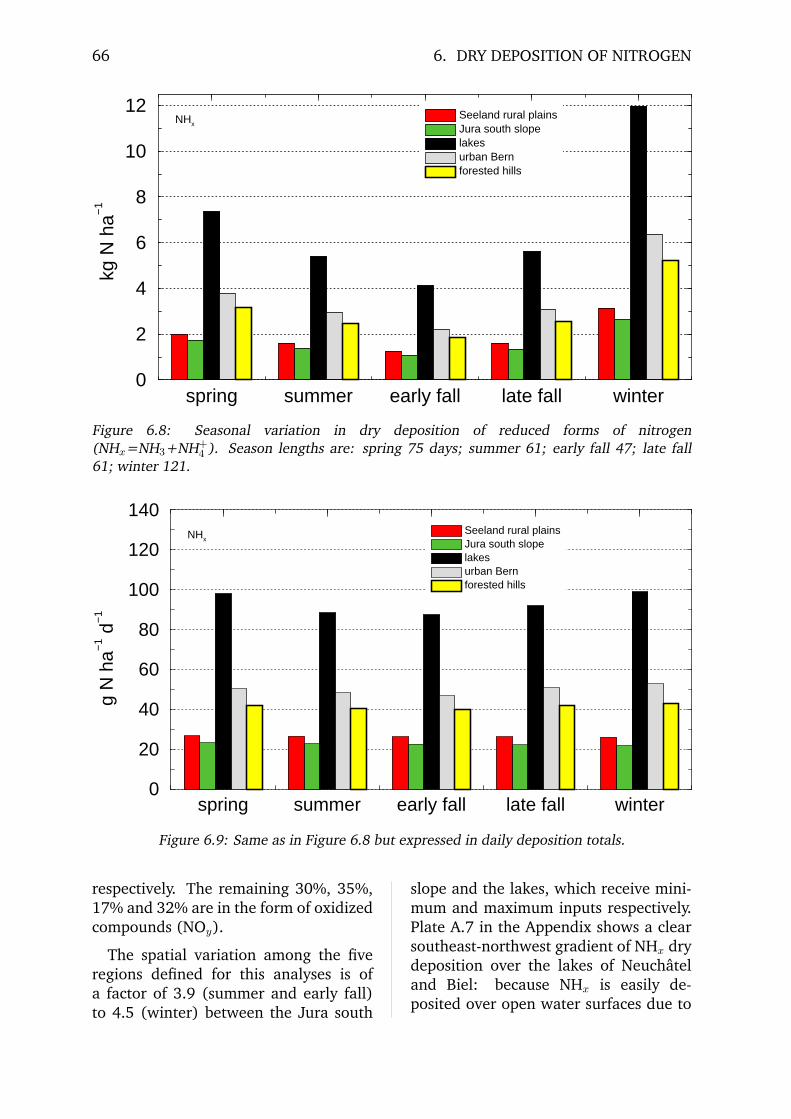
66 6. DRY DEPOSITION OF NITROGEN
spring summer early fall late fall winter0
2
4
6
8
10
12kg
N h
a−1
Seeland rural plainsJura south slopelakesurban Bernforested hills
NHx
Figure 6.8: Seasonal variation in dry deposition of reduced forms of nitrogen(NHx=NH3+NH+
4 ). Season lengths are: spring 75 days; summer 61; early fall 47; late fall61; winter 121.
spring summer early fall late fall winter0
20
40
60
80
100
120
140
g N
ha−
1 d−
1
Seeland rural plainsJura south slopelakesurban Bernforested hills
NHx
Figure 6.9: Same as in Figure 6.8 but expressed in daily deposition totals.
respectively. The remaining 30%, 35%,17% and 32% are in the form of oxidizedcompounds (NOy).
The spatial variation among the fiveregions defined for this analyses is ofa factor of 3.9 (summer and early fall)to 4.5 (winter) between the Jura south
slope and the lakes, which receive mini-mum and maximum inputs respectively.Plate A.7 in the Appendix shows a clearsoutheast-northwest gradient of NHx drydeposition over the lakes of Neuchateland Biel: because NHx is easily de-posited over open water surfaces due to
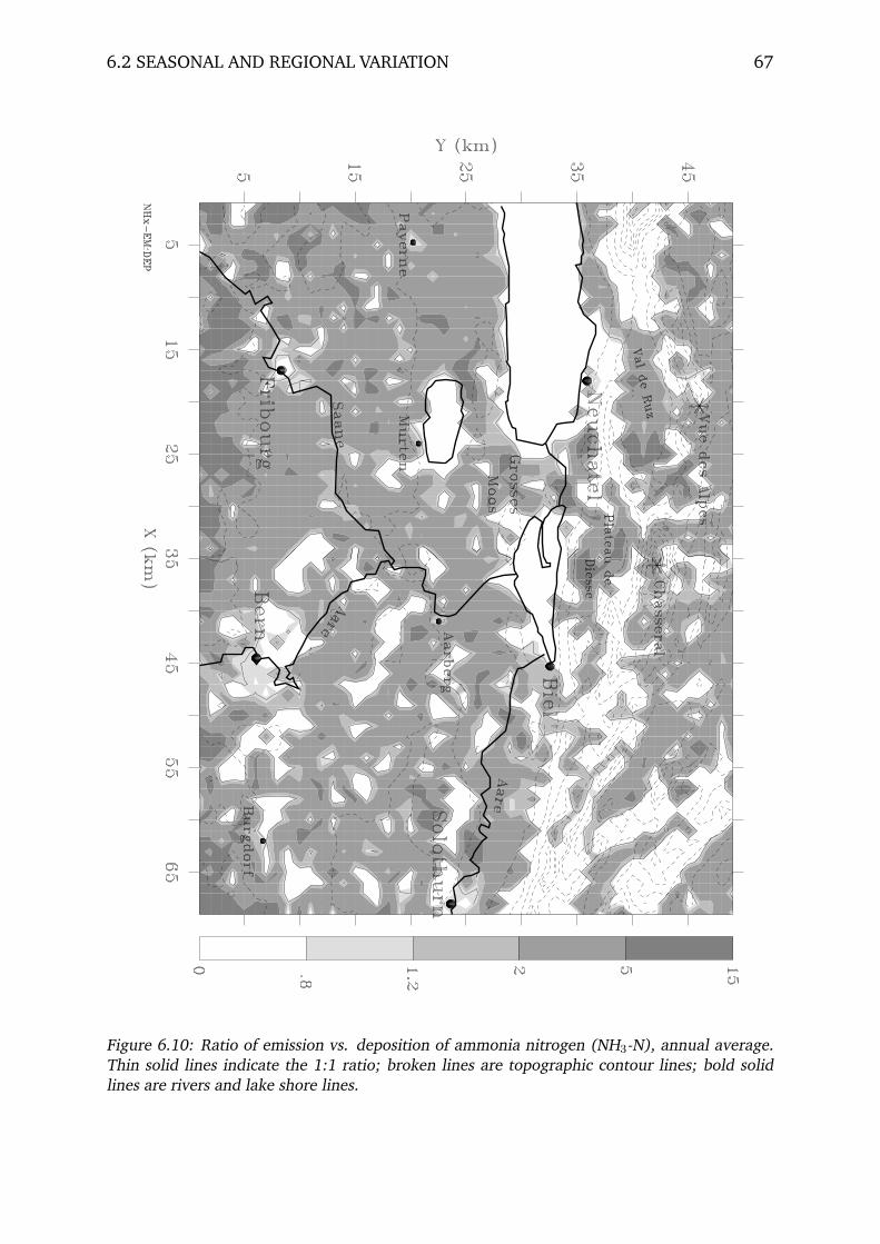
6.2 SEASONAL AND REGIONAL VARIATION 67
Figure 6.10: Ratio of emission vs. deposition of ammonia nitrogen (NH3-N), annual average.Thin solid lines indicate the 1:1 ratio; broken lines are topographic contour lines; bold solidlines are rivers and lake shore lines.

68 6. DRY DEPOSITION OF NITROGEN
Figure 6.11: Ratio of emission vs. deposition of total nitrogen in the study area, annual average.Thin solid lines indicate the 1:1 ratio; broken lines are topographic contour lines; bold solidlines are rivers and lake shore lines.
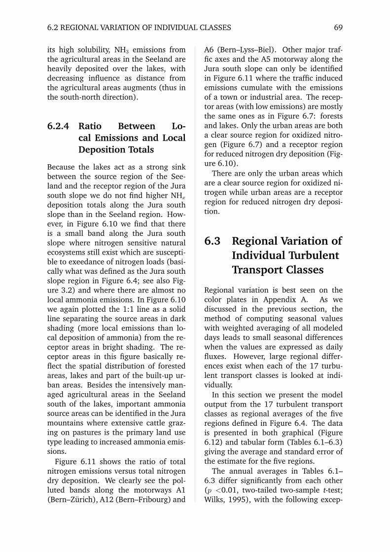
6.2 REGIONAL VARIATION OF INDIVIDUAL CLASSES 69
its high solubility, NH3 emissions fromthe agricultural areas in the Seeland areheavily deposited over the lakes, withdecreasing influence as distance fromthe agricultural areas augments (thus inthe south-north direction).
6.2.4 Ratio Between Lo-cal Emissions and LocalDeposition Totals
Because the lakes act as a strong sinkbetween the source region of the See-land and the receptor region of the Jurasouth slope we do not find higher NHx
deposition totals along the Jura southslope than in the Seeland region. How-ever, in Figure 6.10 we find that thereis a small band along the Jura southslope where nitrogen sensitive naturalecosystems still exist which are suscepti-ble to exeedance of nitrogen loads (basi-cally what was defined as the Jura southslope region in Figure 6.4; see also Fig-ure 3.2) and where there are almost nolocal ammonia emissions. In Figure 6.10we again plotted the 1:1 line as a solidline separating the source areas in darkshading (more local emissions than lo-cal deposition of ammonia) from the re-ceptor areas in bright shading. The re-ceptor areas in this figure basically re-flect the spatial distribution of forestedareas, lakes and part of the built-up ur-ban areas. Besides the intensively man-aged agricultural areas in the Seelandsouth of the lakes, important ammoniasource areas can be identified in the Juramountains where extensive cattle graz-ing on pastures is the primary land usetype leading to increased ammonia emis-sions.
Figure 6.11 shows the ratio of totalnitrogen emissions versus total nitrogendry deposition. We clearly see the pol-luted bands along the motorways A1(Bern–Zurich), A12 (Bern–Fribourg) and
A6 (Bern–Lyss–Biel). Other major traf-fic axes and the A5 motorway along theJura south slope can only be identifiedin Figure 6.11 where the traffic inducedemissions cumulate with the emissionsof a town or industrial area. The recep-tor areas (with low emissions) are mostlythe same ones as in Figure 6.7: forestsand lakes. Only the urban areas are botha clear source region for oxidized nitro-gen (Figure 6.7) and a receptor regionfor reduced nitrogen dry deposition (Fig-ure 6.10).
There are only the urban areas whichare a clear source region for oxidized ni-trogen while urban areas are a receptorregion for reduced nitrogen dry deposi-tion.
6.3 Regional Variation ofIndividual TurbulentTransport Classes
Regional variation is best seen on thecolor plates in Appendix A. As wediscussed in the previous section, themethod of computing seasonal valueswith weighted averaging of all modeleddays leads to small seasonal differenceswhen the values are expressed as dailyfluxes. However, large regional differ-ences exist when each of the 17 turbu-lent transport classes is looked at indi-vidually.
In this section we present the modeloutput from the 17 turbulent transportclasses as regional averages of the fiveregions defined in Figure 6.4. The datais presented in both graphical (Figure6.12) and tabular form (Tables 6.1–6.3)giving the average and standard error ofthe estimate for the five regions.
The annual averages in Tables 6.1–6.3 differ significantly from each other(p <0.01, two-tailed two-sample t-test;Wilks, 1995), with the following excep-

70 6. DRY DEPOSITION OF NITROGEN
Inv1
bIn
v1d
Inv2
b16
/7a
16/7
b16
/7c 26 27 31
a31
b31
cIn
v1a
Inv2
a 0a 0b 0c 30
20
40
60
80
100
kg N
ha−
1 yr−
1
Seeland rural plainJura south slopelakesurban Bernforested hills
total N
Inv1
bIn
v1d
Inv2
b16
/7a
16/7
b16
/7c 26 27 31
a31
b31
cIn
v1a
Inv2
a 0a 0b 0c 30
10
20
30
40
50
kg N
ha−
1 yr−
1
Seeland rural plainJura south slopelakesurban Bernforested hills
NOy
Inv1
bIn
v1d
Inv2
b16
/7a
16/7
b16
/7c 26 27 31
a31
b31
cIn
v1a
Inv2
a 0a 0b 0c 30
10
20
30
40
50
60
70
80
90
kg N
ha−
1 yr−
1
Seeland rural plainJura south slopelakesurban Bernforested hills
NHx
Figure 6.12: Dry deposition totals converted to annual values for the 17 turbulent transportclasses used in our modeling approach. Top: total nitrogen (NOy+NHx); middle: oxidizednitrogen compounds (NOy); bottom: reduced nitrogen compounds (NHx). Error bars indicatestandard errors of the averages.
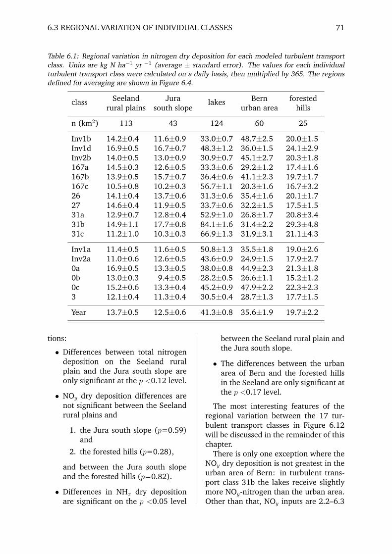
6.3 REGIONAL VARIATION OF INDIVIDUAL CLASSES 71
Table 6.1: Regional variation in nitrogen dry deposition for each modeled turbulent transportclass. Units are kg N ha−1 yr −1 (average ± standard error). The values for each individualturbulent transport class were calculated on a daily basis, then multiplied by 365. The regionsdefined for averaging are shown in Figure 6.4.
Seeland Jura Bern forestedclassrural plains south slope
lakesurban area hills
n (km2) 113 43 124 60 25
Inv1b 14.2±0.4 11.6±0.9 33.0±0.7 48.7±2.5 20.0±1.5Inv1d 16.9±0.5 16.7±0.7 48.3±1.2 36.0±1.5 24.1±2.9Inv2b 14.0±0.5 13.0±0.9 30.9±0.7 45.1±2.7 20.3±1.8167a 14.5±0.3 12.6±0.5 33.3±0.6 29.2±1.2 17.4±1.6167b 13.9±0.5 15.7±0.7 36.4±0.6 41.1±2.3 19.7±1.7167c 10.5±0.8 10.2±0.3 56.7±1.1 20.3±1.6 16.7±3.226 14.1±0.4 13.7±0.6 31.3±0.6 35.4±1.6 20.1±1.727 14.6±0.4 11.9±0.5 33.7±0.6 32.2±1.5 17.5±1.531a 12.9±0.7 12.8±0.4 52.9±1.0 26.8±1.7 20.8±3.431b 14.9±1.1 17.7±0.8 84.1±1.6 31.4±2.2 29.3±4.831c 11.2±1.0 10.3±0.3 66.9±1.3 31.9±3.1 21.1±4.3
Inv1a 11.4±0.5 11.6±0.5 50.8±1.3 35.5±1.8 19.0±2.6Inv2a 11.0±0.6 12.6±0.5 43.6±0.9 24.9±1.5 17.9±2.70a 16.9±0.5 13.3±0.5 38.0±0.8 44.9±2.3 21.3±1.80b 13.0±0.3 9.4±0.5 28.2±0.5 26.6±1.1 15.2±1.20c 15.2±0.6 13.3±0.4 45.2±0.9 47.9±2.2 22.3±2.33 12.1±0.4 11.3±0.4 30.5±0.4 28.7±1.3 17.7±1.5
Year 13.7±0.5 12.5±0.6 41.3±0.8 35.6±1.9 19.7±2.2
tions:
• Differences between total nitrogendeposition on the Seeland ruralplain and the Jura south slope areonly significant at the p <0.12 level.
• NOy dry deposition differences arenot significant between the Seelandrural plains and
1. the Jura south slope (p=0.59)and
2. the forested hills (p=0.28),
and between the Jura south slopeand the forested hills (p=0.82).
• Differences in NHx dry depositionare significant on the p <0.05 level
between the Seeland rural plain andthe Jura south slope.
• The differences between the urbanarea of Bern and the forested hillsin the Seeland are only significant atthe p <0.17 level.
The most interesting features of theregional variation between the 17 tur-bulent transport classes in Figure 6.12will be discussed in the remainder of thischapter.
There is only one exception where theNOy dry deposition is not greatest in theurban area of Bern: in turbulent trans-port class 31b the lakes receive slightlymore NOy-nitrogen than the urban area.Other than that, NOy inputs are 2.2–6.3

72 6. DRY DEPOSITION OF NITROGEN
Table 6.2: Regional variation in dry deposition of oxidized compounds (NOy) for each modeledturbulent transport class. Units are kg N ha−1 yr −1 (average ± standard error). The values foreach individual turbulent transport class were calculated on a daily basis, then multiplied by365. The regions defined for averaging are shown in Figure 6.4.
Seeland Jura Bern forestedclassrural plains south slope
lakesurban area hills
n (km2) 113 43 124 60 25
Inv1b 5.6±0.1 5.8±0.7 7.6±0.1 27.8±1.7 6.1±0.4Inv1d 7.2±0.1 8.7±0.4 9.3±0.1 19.7±0.8 7.3±0.2Inv2b 4.3±0.1 4.5±0.5 5.6±0.2 26.1±2.4 4.5±0.2167a 3.8±0.1 4.6±0.3 4.9±0.1 13.4±0.9 3.3±0.2167b 5.3±0.2 7.3±0.5 13.5±0.3 27.6±1.9 7.5±0.6167c 3.2±0.1 3.2±0.1 7.0±0.1 7.7±0.3 3.5±0.326 4.2±0.1 4.6±0.4 4.5±0.1 12.8±0.7 4.5±0.227 3.3±0.1 3.0±0.3 4.5±0.1 12.3±0.9 2.8±0.131a 4.2±0.1 4.6±0.3 10.9±0.2 13.2±0.6 5.8±0.631b 4.7±0.2 6.4±0.4 14.7±0.2 14.1±0.8 7.5±0.731c 2.0±0.0 1.7±0.1 4.3±0.1 7.4±0.5 2.0±0.2
Inv1a 2.5±0.0 3.8±0.2 3.1±0.1 15.7±1.0 2.7±0.1Inv2a 1.9±0.0 3.3±0.2 3.3±0.1 8.8±0.5 2.2±0.10a 4.9±0.1 3.6±0.3 7.6±0.2 25.2±1.9 4.4±0.20b 3.8±0.1 3.2±0.4 4.6±0.1 11.4±0.7 3.1±0.10c 4.8±0.1 4.1±0.3 6.6±0.1 25.6±1.4 4.6±0.23 3.0±0.1 3.0±0.2 5.0±0.1 8.8±0.4 3.5±0.2
Year 4.1±0.1 4.3±0.3 6.8±0.1 17.2±1.1 4.4±0.3
times higher in the urban area of Bernthan in the forested hills or the ruralplains of the Seeland.
Forested hills in the Seeland generallyreceive more total and reduced nitro-gen, independent of the turbulent trans-port conditions. Oxidized nitrogen how-ever is only dry deposited in excess ofthe amounts received in the Seeland ru-ral plains in turbulent transport classes16/7b, 31a, and 31b. These are classeswith prevailing northeasterly flow atlower altitudes in the Seeland, but ex-cluding the subclasses with the strongestor very weak winds (in the case of 16/7).This dependence on wind speed is seenin all NOy deposition amounts in theclasses 16/7 and 31: the subclasses with
moderate wind speed (16/7b and 31b)show the highest dry deposition of NOy,while at higher wind speeds the depo-sition is among the lowest (16/7c and31c).
The Jura south slope region receivesmore total nitrogen dry deposition thanthe Seeland rural plains in turbulenttransport classes 16/7b (+13%), 31b(+19%), and Inv2a (+15%). Andthe input is equal to within 10% ofthe input received in the Seeland ru-ral plains with turbulent transport condi-tions Inv1d, Inv2b, 16/7c, 26, 31a, 31c,Inv1a, 0c and 3.
Forested hills in the Seeland receive25% (16/7b) to 105% (31c) more totalnitrogen than the Jura south slope. The

6.3 REGIONAL VARIATION OF INDIVIDUAL CLASSES 73
Table 6.3: Regional variation in dry deposition of reduced nitrogen compounds (NHx) for eachmodeled turbulent transport class. Units are kg N ha−1 yr −1 (average ± standard error).The values for each individual turbulent transport class were calculated on a daily basis, thenmultiplied by 365. The regions defined for averaging are shown in Figure 6.4.
Seeland Jura Bern forestedclassrural plains south slope
lakesurban area hills
n (km2) 113 43 124 60 25
Inv1b 8.5±0.3 5.9±0.3 25.4±0.7 20.8±1.6 13.9±1.3Inv1d 9.7±0.5 7.9±0.3 39.0±1.2 16.3±1.3 16.7±2.8Inv2b 9.7±0.4 8.5±0.5 25.3±0.6 19.0±1.2 15.8±1.7167a 10.7±0.3 8.0±0.3 28.4±0.6 15.8±0.8 14.1±1.5167b 8.6±0.3 8.4±0.3 22.9±0.4 13.5±0.7 12.1±1.1167c 7.3±0.7 7.0±0.2 49.7±1.1 12.6±1.5 13.2±3.026 10.0±0.4 9.2±0.4 26.8±0.6 22.6±1.2 15.6±1.527 11.3±0.4 8.8±0.3 29.1±0.5 19.9±1.1 14.7±1.431a 8.8±0.6 8.2±0.2 42.0±0.9 13.5±1.4 15.0±2.831b 10.2±0.9 11.3±0.5 69.5±1.5 17.3±1.9 21.8±4.231c 9.2±1.0 8.5±0.3 62.6±1.3 24.5±3.0 19.0±4.1
Inv1a 8.9±0.5 7.8±0.4 47.7±1.3 19.8±1.6 16.2±2.5Inv2a 9.0±0.5 9.3±0.4 40.2±0.9 16.1±1.4 15.7±2.60a 12.0±0.5 9.7±0.4 30.3±0.8 19.7±0.9 16.9±1.60b 9.2±0.3 6.2±0.2 23.7±0.5 15.2±0.8 12.1±1.10c 10.4±0.6 9.1±0.3 38.6±0.9 22.3±1.3 17.7±2.13 9.1±0.4 8.3±0.3 25.5±0.4 19.9±1.0 14.2±1.3
Year 9.6±0.5 8.2±0.3 34.5±0.8 18.4±1.3 15.2±1.9
amount of total nitrogen dry depositedto the lakes is 2–6 fold the amount de-posited on the Seeland rural plains. Thisis mainly due to the solubility of NHx inwater which increases NHx deposition tothe lake by a factor of 2.5–6.8 comparedwith the Seeland rural plains, and a fac-tor of 2.7–7.3 compared with the Jurasouth slope. These are large regional dif-ferences within a horizontal distance ofonly 10–20 km!
The level of nitrogen deposition to thelakes revealed to be one of the key fea-tures in this study region. At low andhigh wind speeds of the classes wherewind speed is an additional classifier(16/7, 31, and 0), the NHx depositionis enhanced compared to moderate wind
speeds, except in the case of class 31b.This indicates that there is a complexdynamical interation between the turbu-lent transport in the atmosphere and theammonia deposition to the lakes. TheNHx dry deposition to the lakes variesby a factor of 3.0 between the turbulenttransport class with the lowest (16/7b)and highest (31b) inputs. In the otherfour regions it varies only by a factor 1.6,1.9, 1.9, and 1.8 for the Seeland ruralplain, the Jura south slope, the urbanarea of Bern, and the forested hills re-spectively. Larger variations than thoseof NHx deposition over the lakes are onlyfound for the NOy deposition over thelakes and in the urban area of Bern,where there is a factor of 4.7 and 3.8

74 6. DRY DEPOSITION OF NITROGEN
variation, respectively.The classes with pronounced thermal
inversions have a strong influence onNOy deposition in the urban area ofBern if surface wind direction is fromthe Northeast (classes Inv1b, Inv1d, andInv2b). When wind is from the South-west (Inv1a, Inv2a), the NOy depositionis still the highest in the urban area ofBern but with much lower absolute val-ues than under northeasterly flow. Thethermal inversions therefore do not seemto be the dominating factor when windsare from the southwest, as can be seen inthe values of classes 0a–0c which showhigher NOy inputs than the two classeswith a strong thermal inversion.
In 11 out of the 17 classes the lakesreceive more nitrogen by dry deposi-tion than the urban area of Bern. Al-though it was readily discussed that sucha comparison is not quite addressing thesame nitrogen components (NHx overthe lakes versus a combination of 48%NOy and 52% NHx in the urban area)it is a very useful statistic to get a han-dle on dry deposition of total nitrogen:in 65% of the weather conditions consid-ered in this study the lakes receive morenitrogen by dry deposition than the ur-ban area of Bern.
7. Wet Deposition of Nitrogen
7.1 Introduction
Wet deposition was treated separatelydue to the fact that Metphomod wasoriginally designed for modeling photo-smog conditions and thus does not in-clude a cloud physics and precipitationmodule in the version 1.1 used here.
To estimate the contribution of wetdeposition to annual nitrogen deposi-tion, we employed an experimental ap-proach in combination with data fromthe NABEL monitoring site at Payerne,where wet deposition is sampled on adaily basis. Our own mesurements doneby Gempeler (1997) covered five sites inthe study area to address spatial varia-tion in wet deposition during the grow-ing season. New wet-only samplers weredeveloped which run on battery powerand which use a new rain droplet detec-tion sensor developed at the Institute ofGeography at the University of Bern byMr. Jurg Schenk.
For a long-term comparison unpub-lished data (courtesy of Jurg Fuhrer, Fed-eral Research Institute for Environmen-tal Protection and Agriculture, Liebefeld-Bern) from three locations (Liebefeld-Bern; Belpmoos close to the Bern air-port; and Langenberg) were analysedand compared with Marion Gempeler’sdata.
7.2 Working Hypotheses
It is generally assumed that wet deposi-tion is a larger-scale phenomenon thandry deposition. Even if Metphomod were
able to model precipitation events rea-sonably, the question of the size of themodel domain would still remain. Onthe other hand, regional variation in wetdeposition is assumed to be much lessimportant than the regional variation indry deposition. Our experimental ap-proach thus was based on the followinghypotheses:
1. There is an altitudinal gradient inwet deposition nitrogen input dueto increasing precipitation amountswith higher altitude.
2. Regional variation is largest duringconvective (summertime) precipita-tion events. The horizontal extentof convective clouds is small, andupdrafts are strong, such that pol-luted air is drawn into the clouds.In this way, concentrations increasein the droplets of convective clouds,which results in increasing nitrogenconcentrations with increasing pre-cipitation amounts (Bloxham et al.,1984).
3. There is no regional variation dur-ing advective (non-convective) pre-cipitation events (e. g. warm fronts,late fall and early spring precipi-tation). The horizontal extent ofclouds is 100 km and more in thiscase, and precipitation is more orless evenly distributed over largeareas. Updrafts in the cloudsare only weak and therefore small-scale variation in nitrogen concen-trations is assumed to be unim-portant in the cloud water. Ni-
75
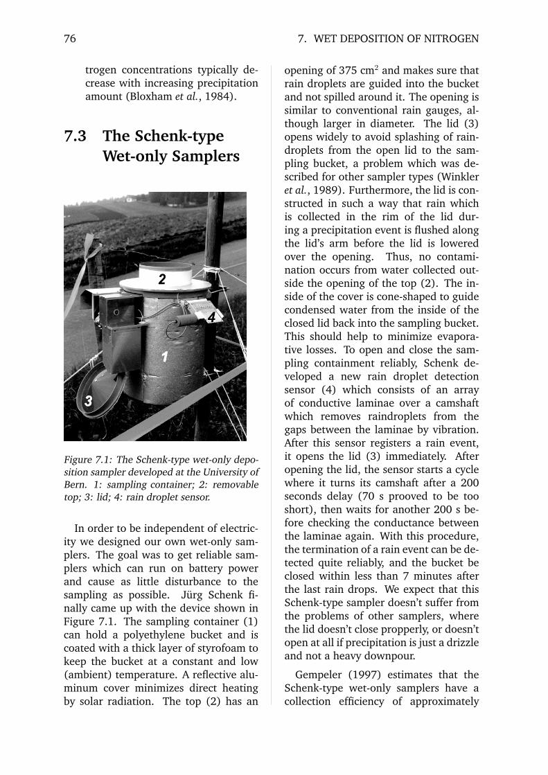
76 7. WET DEPOSITION OF NITROGEN
trogen concentrations typically de-crease with increasing precipitationamount (Bloxham et al., 1984).
7.3 The Schenk-typeWet-only Samplers
Figure 7.1: The Schenk-type wet-only depo-sition sampler developed at the University ofBern. 1: sampling container; 2: removabletop; 3: lid; 4: rain droplet sensor.
In order to be independent of electric-ity we designed our own wet-only sam-plers. The goal was to get reliable sam-plers which can run on battery powerand cause as little disturbance to thesampling as possible. Jurg Schenk fi-nally came up with the device shown inFigure 7.1. The sampling container (1)can hold a polyethylene bucket and iscoated with a thick layer of styrofoam tokeep the bucket at a constant and low(ambient) temperature. A reflective alu-minum cover minimizes direct heatingby solar radiation. The top (2) has an
opening of 375 cm2 and makes sure thatrain droplets are guided into the bucketand not spilled around it. The opening issimilar to conventional rain gauges, al-though larger in diameter. The lid (3)opens widely to avoid splashing of rain-droplets from the open lid to the sam-pling bucket, a problem which was de-scribed for other sampler types (Winkleret al., 1989). Furthermore, the lid is con-structed in such a way that rain whichis collected in the rim of the lid dur-ing a precipitation event is flushed alongthe lid’s arm before the lid is loweredover the opening. Thus, no contami-nation occurs from water collected out-side the opening of the top (2). The in-side of the cover is cone-shaped to guidecondensed water from the inside of theclosed lid back into the sampling bucket.This should help to minimize evapora-tive losses. To open and close the sam-pling containment reliably, Schenk de-veloped a new rain droplet detectionsensor (4) which consists of an arrayof conductive laminae over a camshaftwhich removes raindroplets from thegaps between the laminae by vibration.After this sensor registers a rain event,it opens the lid (3) immediately. Afteropening the lid, the sensor starts a cyclewhere it turns its camshaft after a 200seconds delay (70 s prooved to be tooshort), then waits for another 200 s be-fore checking the conductance betweenthe laminae again. With this procedure,the termination of a rain event can be de-tected quite reliably, and the bucket beclosed within less than 7 minutes afterthe last rain drops. We expect that thisSchenk-type sampler doesn’t suffer fromthe problems of other samplers, wherethe lid doesn’t close propperly, or doesn’topen at all if precipitation is just a drizzleand not a heavy downpour.
Gempeler (1997) estimates that theSchenk-type wet-only samplers have acollection efficiency of approximately

7.5 SITES 77
97% and collect all liquid precipitationwhich falls at an intensity of at least0.1 mm h−1. She estimates that themeasurements are representative within±5–15% for the sampling location, thusidentical to conventional precipitationgauges (Reiss et al., 1992).
7.4 Methods
The buckets from our wet-only depo-sition samplers were collected weeklyfrom 26 July to 28 November 1995 andfrom 10 April to 10 June 1996. The to-tal precipitation collected and the con-centration of nitrate (NO−
3 ), ammonium(NH+
4 ), sulfate (SO2−4 ), chlorine (Cl−),
and acidity (H+ and pH) were deter-mined in the laboratories of the Fed-eral Research Institute for Environmen-tal Protection and Agriculture, Liebefeld-Bern. Batches from several weeks wereprocessed at a time, and samples werestored at a temperature below 4◦C be-fore processing. According to Mulleret al. 1982, Gempeler (1997) estimatesthat concentration losses might be in theorder of 18% between collection andprocessing. Together with the samplingefficiency of the wet-only samplers weassume that our wet deposition mea-surements are integrating approximately80% of the true nitrogen wet deposition.
Sampling buckets were cleaned withde-ionized water, then filled with 0.1-molar chlorine acide (HCl) for severaldays for conditioning. Then they wereflushed with de-ionized water and storedin de-ionized water before use.
The same procedure was carried outwith the samplers when they were notin use. In the field, the lid was flushedwith de-ionized water after removal ofthe bucket and before installing the new,empty bucket to eliminate the memory-effect (Winkler et al., 1989).
Total precipitation was determined by
weighing the buckets, then the weightof each bucket was subtracted. Then, asmall fraction of the solution was sep-arated from the bulk for determiningacidity (pH) with an Orion 901 ion an-alyzer. Approximately 50 ml were fil-tered with a syringe through a 45 µm fil-ter, then stored in the refrigerator. Therest of the solution was discharged, ifthe weekly precipitation exceeded theamount needed for the analyses.
The nitrate, sulfate and chlorine an-ions were analyzed with a Dionex ionchromatograph. Ammonia was deter-mined photometrically.
7.5 Sites
The locations where wet deposition (Fig-ure 7.2) were chosen in order to givea rough transect across the Seeland ru-ral plains and the lower elevations onthe Jura south slope (where we expectthat an exceedance in nitrogen deposi-tion has the largest potential effect onpresent ecosystem types). The five sitesrun by Gempeler (1997) are listed inTable 7.1 together with four additionalsites from which long-term data setswere available.
Kerzersmoos (435 m) and Siselen(439 m) represent typical agriculturalareas in the Seeland rural plain re-gion. Kerzersmoos is also the focus ofthe BAT project (Regional Budgets ofAtmospheric Trace Gases) of the Fed-eral Research Institute for Environmen-tal Protection and Agriculture, Liebefeld-Bern , the University of Bern and theSwiss Federal Institute of Technology(ETH) Zurich.
Jolimont (562 m) is on top of Jolimonthill in an agriculturally used forest clear-ing close to a farmhouse and is sur-rounded by deciduous and mixed for-est. This location is representative forthe forested hills in the Seeland region.

78 7. WET DEPOSITION OF NITROGEN
Figure 7.2: Location of sites of wet-only deposition samplers.
Le Landeron (620 m) and Lignieres(875 m) were selected to assess the oro-graphic and altitudinal effect which weexpect to find along the Jura south slope.
7.6 Scaling up to AnnualWet DepositionEstimates
There are numerous methods via whichto scale up from short-term measure-ments to annual values. We selectedtwo methods for this study, based onthe experience we gained from our datameasured in the Seeland, and basedon the data availability for scaling up.
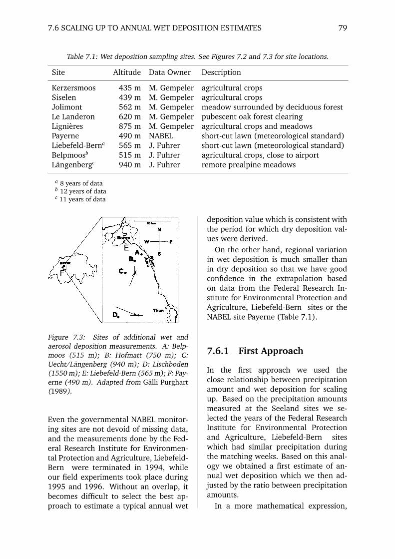
7.6 SCALING UP TO ANNUAL WET DEPOSITION ESTIMATES 79
Table 7.1: Wet deposition sampling sites. See Figures 7.2 and 7.3 for site locations.
Site Altitude Data Owner Description
Kerzersmoos 435 m M. Gempeler agricultural cropsSiselen 439 m M. Gempeler agricultural cropsJolimont 562 m M. Gempeler meadow surrounded by deciduous forestLe Landeron 620 m M. Gempeler pubescent oak forest clearingLignieres 875 m M. Gempeler agricultural crops and meadowsPayerne 490 m NABEL short-cut lawn (meteorological standard)Liebefeld-Berna 565 m J. Fuhrer short-cut lawn (meteorological standard)Belpmoosb 515 m J. Fuhrer agricultural crops, close to airportLangenbergc 940 m J. Fuhrer remote prealpine meadows
a 8 years of datab 12 years of datac 11 years of data
Er
Fr
Figure 7.3: Sites of additional wet andaerosol deposition measurements. A: Belp-moos (515 m); B: Hofmatt (750 m); C:Uecht/Langenberg (940 m); D: Lischboden(1550 m); E: Liebefeld-Bern (565 m); F: Pay-erne (490 m). Adapted from Galli Purghart(1989).
Even the governmental NABEL monitor-ing sites are not devoid of missing data,and the measurements done by the Fed-eral Research Institute for Environmen-tal Protection and Agriculture, Liebefeld-Bern were terminated in 1994, whileour field experiments took place during1995 and 1996. Without an overlap, itbecomes difficult to select the best ap-proach to estimate a typical annual wet
deposition value which is consistent withthe period for which dry deposition val-ues were derived.
On the other hand, regional variationin wet deposition is much smaller thanin dry deposition so that we have goodconfidence in the extrapolation basedon data from the Federal Research In-stitute for Environmental Protection andAgriculture, Liebefeld-Bern sites or theNABEL site Payerne (Table 7.1).
7.6.1 First Approach
In the first approach we used theclose relationship between precipitationamount and wet deposition for scalingup. Based on the precipitation amountsmeasured at the Seeland sites we se-lected the years of the Federal ResearchInstitute for Environmental Protectionand Agriculture, Liebefeld-Bern siteswhich had similar precipitation duringthe matching weeks. Based on this anal-ogy we obtained a first estimate of an-nual wet deposition which we then ad-justed by the ratio between precipitationamounts.
In a more mathematical expression,
80 7. WET DEPOSITION OF NITROGEN
this corresponds to the equation
FN,annual =
t2∑i=t1
pi,j
t2∑i=t1
pi,refk
·FN,annualk,ref , (7.1)
where FN,annual is the annual nitrogenwet deposition flux estimate for the See-land, pi,j is the precipitation amountat location j in the Seeland during theweek of year i, pi,refk is the precipitationamount during the same week of year kat some reference long-term station, andFN,annualk,ref is the corresponding annualnitrogen wet deposition flux at this ref-erence station during the same year k. t1and t2 are the first and last week of a spe-cific measuring campaign in the Seeland.
7.6.2 Second Approach
In the second approach we take the long-term values from the Federal ResearchInstitute for Environmental Protectionand Agriculture, Liebefeld-Bern sites andestimate the fraction of annual nitrogenwet deposition that occurs during theweeks of the year for which measure-ments from the Seeland study area areavailable. Using this fraction we scaleup the measured wet deposition to anaverage annual deposition without con-sidering the amount of precipitation. Inaddition to that, we adjust this estimatewith a factor which takes the samplingefficiency of our wet-only samplers intoaccount. It has been stated before thatthe concentration in precipitation wateris greatest at the very beginning of a pre-cipitation event in the case of summer-time convective precipitation. Due to thetime lag between the moment when therain droplet sensor detects the beginningof an event and the time when the sam-pling bucket is uncovered and fully ex-posed to the rain, an important fractionof wet deposition is not correctly col-lected. And during drizzling rain events
the buckets may stay closed, so that weestimate an overall sampling efficiencyof about 80%. Therefore, we add 25%to the wet deposition estimates obtainedin that way.
Again, in a more formal way, this maybe expressed by the equation
FN,annual =t2∑
i=t1
FN,i,j ·FN,annual,reft2∑
i=t1
FN,i,ref
· 1ξ.
(7.2)Here, FN,i,ref denotes the long-term av-erage nitrogen wet deposition flux dur-ing week i at some reference stationof the Federal Research Institute forEnvironmental Protection and Agricul-ture, Liebefeld-Bern, and FN,annual,ref isthe long-term average nitrogen wet de-position at the same station. ξ is the sam-pling efficiency which we estimate to beξ = 0.8.
7.6.3 Comparison Betweenthe two Approaches
We assume that the first approach yieldsa good estimate of total annual nitro-gen wet deposition in the Seeland for theyears with data. However, to be com-patible with the time period chosen fordry deposition modeling, we are rathermore interested in a good estimate for anaverage year, therefore we suggest thatthe second approach gives an estimatewhich is directly comparable to the drydeposition totals.
7.7 Results
Wet deposition of nitrogen shows greatinterannual variability, therefore mea-suring periods of 10 years or more arerequired to get a good estimate of long-term nitrogen inputs via precipitation.We knew that it is impossible to get agood experimental estimate of wet de-position within the three year funding
7.7 RESULTS 81
Table 7.2: Estimation of annual nitrogenwet deposition based on approach 1 (Section7.6.1). Precipitation in 1995 was most sim-ilar to the 1990 IUL data, while 1994 wasused for analogy with our 1996 data. Unitsare kg N ha−1 yr−1.
Year NO3-N NH4-N total N
1995 3.2–3.7 6.5–7.0 9.7–10.71996 2.5–2.8 4.2 6.7–7.0
average 3.0 5.5 8.5
period of this study. Therefore, ourapproach basically addressed the ques-tion of how to derive a reasonable esti-mate for our study area based on long-term measurements available from out-side the region.
Modelling of wet deposition on the re-gional scale was not possible with Met-phomod, mainly due to the fact that thespatial scale of gaseous transport, drydeposition and photochemical transfor-mation is at least one order of magni-tude smaller than the spatial scale ofcloud growth, transport, and precipita-tion, which govern wet deposition.
Gempeler’s (1997) field campaigns in1995 and 1996 cover 16 and 12 weeksof a full year’s cycle, respectively, whichis roughly 54% of a full year. This timeperiod totals 65% of annual precipitationand 66% of annual nitrogen wet deposi-tion (Table 7.3). Therefore, we are quiteconfident that scaling up from this dataset to an annual total is straightforwardand annual estimates should be reason-able despite the lack of long-term mea-surements from within the study area.
With approach 1 (Section 7.6.1) a to-tal nitrogen wet deposition of 8.5 kg perhectar per year is estimated for the studyarea (Table 7.2). 35% of this nitrogenis input in oxidized form (nitrate), and65% in reduced form (ammonium).
Aerosol particles consist mainly of am-
monium nitrate NH4NO3 and ammo-nium sulfate (NH4)2SO4. Thus, the ratioof nitrate versus ammonium depositiongives an indication of the origin of thenitrogen in the wet deposition. If onlyammonium nitrate were present, the wetdeposition of nitrogen should be 50% ni-trate and 50% ammonium. If only am-monium sulfate were present, the the-oretical values would be 0% for nitrateand 100% for ammonium. Therefore,the lower the sulfur emissions and depo-sitions in a region, the higher the frac-tion of nitrogen which is deposited in re-duced form as ammonium. This is con-sistent with the values measured for sul-fate in the Seeland by Gempeler (1997).Based on her measurements we estimateannual sulfur wet deposition to be in theorder of 4–4.5 kg S per hectar. This valueis lower than estimates for other simi-lar locations in industrialized countriesin Europe, and reflects the success in thenational sulfur emission reduction strat-egy. Sulfur wet deposition is not a mainproblem for the region and we thereforedo not go further into detailed discus-sion of sulfur deposition. However, sul-fur is also contributing to the acidifyinginputs which are still exceeding the criti-cal loads in the forests of the Seeland re-gion. All data from our study region onsulfate, chlorine and hydrogen (pH) in-puts are tabulated in Gempeler (1997).
Due to the rather wet conditions in1995 we assume that this estimate israther a high estimate for the long-termwet deposition input in the Seeland. Thevalues derived with the second approach(Section 7.6.2) are smaller (Table 7.4),but probably more representative for thelong-term annual total. The number ofsamples per site was too small to signifi-cantly detect regional differences in wetdeposition. One reason is also that just afew missing (weekly) values from differ-ent weeks at different sites dramaticallyreduce the statistical basis for an anal-
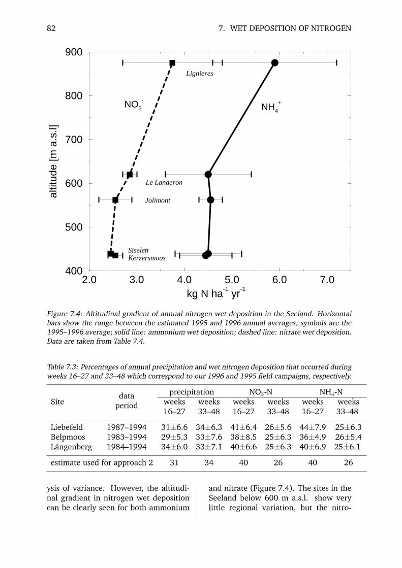
82 7. WET DEPOSITION OF NITROGEN
2.0 3.0 4.0 5.0 6.0 7.0kg N ha
-1 yr
-1
400
500
600
700
800
900al
titud
e [m
a.s
.l]
NO3
-
NH4
+
Lignieres
Le Landeron
Jolimont
SiselenKerzersmoos
Figure 7.4: Altitudinal gradient of annual nitrogen wet deposition in the Seeland. Horizontalbars show the range between the estimated 1995 and 1996 annual averages; symbols are the1995–1996 average; solid line: ammonium wet deposition; dashed line: nitrate wet deposition.Data are taken from Table 7.4.
Table 7.3: Percentages of annual precipitation and wet nitrogen deposition that occurred duringweeks 16–27 and 33–48 which correspond to our 1996 and 1995 field campaigns, respectively.
precipitation NO3-N NH4-NSite
dataweeks weeks weeks weeks weeks weeksperiod16–27 33–48 16–27 33–48 16–27 33–48
Liebefeld 1987–1994 31±6.6 34±6.3 41±6.4 26±5.6 44±7.9 25±6.3Belpmoos 1983–1994 29±5.3 33±7.6 38±8.5 25±6.3 36±4.9 26±5.4Langenberg 1984–1994 34±6.0 33±7.1 40±6.6 25±6.3 40±6.9 25±6.1
estimate used for approach 2 31 34 40 26 40 26
ysis of variance. However, the altitudi-nal gradient in nitrogen wet depositioncan be clearly seen for both ammonium
and nitrate (Figure 7.4). The sites in theSeeland below 600 m a.s.l. show verylittle regional variation, but the nitro-
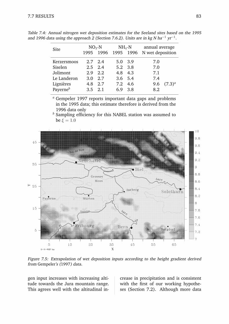
7.7 RESULTS 83
Table 7.4: Annual nitrogen wet deposition estimates for the Seeland sites based on the 1995and 1996 data using the approach 2 (Section 7.6.2). Units are in kg N ha−1 yr−1.
NO3-N NH4-N annual averageSite1995 1996 1995 1996 N wet deposition
Kerzersmoos 2.7 2.4 5.0 3.9 7.0Siselen 2.5 2.4 5.2 3.8 7.0Jolimont 2.9 2.2 4.8 4.3 7.1Le Landeron 3.0 2.7 3.6 5.4 7.4Lignieres 4.8 2.7 7.2 4.6 9.6 (7.3)a
Payerneb 3.5 2.1 6.9 3.8 8.2
a Gempeler 1997 reports important data gaps and problemsin the 1995 data; this estimate therefore is derived from the1996 data only
b Sampling efficiency for this NABEL station was assumed tobe ξ = 1.0
Figure 7.5: Extrapolation of wet deposition inputs according to the height gradient derivedfrom Gempeler’s (1997) data.
gen input increases with increasing alti-tude towards the Jura mountain range.This agrees well with the altitudinal in-
crease in precipitation and is consistentwith the first of our working hypothe-ses (Section 7.2). Although more data

84 7. WET DEPOSITION OF NITROGEN
would be needed to thoroughly test thehypothesis of an altitudinal dependencyin wet deposition, we can state that thisis rather a question of statistics and thatit is not unlikely that longer time serieswith less data gaps from all five Seelandsites would lead to statistically signifi-cant differences in altitudinal variationsof wet deposition.
However, hypotheses 2 and 3 (Sec-tion 7.2) remain open. Gempeler (1997)suggests that an experimental conceptto measure single precipitation eventsrather than weekly totals would be nec-essary to be able to clearly separateconvective from advective precipitationevents.
In Table 7.4 our estimate for an aver-age annual nitrogen wet deposition totalis 7.0 kg nitrogen per hectar in the See-land and about 7.4 kg nitrogen per hec-tar on the south slope of the Jura. Thisis roughly 18% below the estimate ob-tained via approach 1. From this we canconclude that we could derive a reason-able estimate of annual nitrogen wet de-position in the Seeland just by measur-ing precipitation, then scaling up withapproach 1, or by taking the values mea-sured at the NABEL site in Payerne (Ta-ble 7.4) which differ by only 15% fromthe values obtained in our study area byGempeler (1997). To increase our con-fidence in the altitudinal gradient, ad-ditional measurements would be neces-sary along the Jura south slope. A newproject that is currently operating willfocus on this altitudinal gradient mea-sured during summer 1998 precipitationevents (diploma thesis of Mrs DanielaNowak).
For regional extrapolation we onlyused the observed altitudinal gradientand no horizontal variation at constant
elevation. With the simple equation
FN (z) =7.0 : z < 620
7.0 + 0.0102 · (z − 620) : 620 ≤ z ≤ 9009.9 : z > 900
(7.3)
where z is altitude in m a.s.l. and FN
is annual wet deposition of nitrogen inkg N ha−1 yr−1 we produced Figure 7.5.

8. Dry Deposition of Aerosol Particles
8.1 Introduction
So far only dry deposition of nitrogen-containing trace gases and wet deposi-tion have been discussed. Dry depositionof aerosol particles were not included be-cause Metphomod only models gaseousphase chemistry. Particulate matter isnot represented in the model.
Because we found that wet depositionin the Seeland was similar to the valuesobtained in the Aare river valley south ofBern we assume that the same sites willgive us reasonable estimates for aerosoldry deposition as well. We therefore re-analized original and unpublished datafrom Galli Purghart (1989) to obtain anestimate of aerosol nitrogen depositionin our study area.
8.2 Data used
Brigitte Galli sampled dry particulatedeposition (large aerosol particles) andmeasured aerosol particle concentrationon a weekly basis using a Berner cas-cade impactor which fractionates 9 dif-ferent aerosol sizes. The data recordsof the dry particulate deposition at thefour sites Belpmoos, Hofmatt, Uecht andLischboden in the Gurbe river valley areshown in Figure 8.1. The sites corre-spond with the wet deposition sites men-tioned in Chapter 7.
The sampling of dry particulate depo-sition was performed by a dry-only sam-pling bucket which has its lid closed dur-ing precipitation events. Thus, we ex-pect that only the very large particles
are found in such a sample, and that to-tal aerosol dry deposition must be com-posed of the two components: (1) sedi-mentation of large particles, and (2) im-paction and diffusion of smaller parti-cles. For (1) we used the unpublisheddata of B. Galli, while we use FN,i =CN · vd for (2), where FN,i is the nitro-gen flux of small particles (aerosol sizes<8 µm were used), CN is the nitrogenconcentration of the aerosols derived bymultiplying measured aerosol mass witha nitrogen factor (see Section 8.4.1), andvd is the deposition velocity (sedimenta-tion, impaction and diffusion) describedin Section 8.4.2. Although there is someoverlap between the sedimentation mea-surements (1) and our calculation of thedeposition of small particles (2; for par-ticles >1 µm), we expect the resultingerror to be small compared to the uncer-tainty in sedimentation measurementsand estimates of nitrogen content anddeposition velocity.
We only used the 7 smallest fractionsof Galli’s 9 size fractions for this analysisbecause the performance of a Berner im-pactor for particle sizes >8 µm is uncer-tain, and because these two largest sizefractions are believed to have most over-lap with what was already sampled viathe dry-only sampling buckets.
85

86 8. DRY DEPOSITION OF AEROSOL PARTICLES
0 10 20 30 40 50 60week
0
5
100 10 20 30 40 50 60
0
5
10
m
g N
m−
2 wee
k−1
0 10 20 30 40 50 600
5
10
150 10 20 30 40 50 60
05
10152025
x x
Belpmoos
Hofmatt
Uecht
Lischboden
Figure 8.1: Weekly aerosol dry deposition data measured from 16 July 1985–16 September1986 at four sites in a height profile in the Bernese Prealps (see Figure 7.3). Dashed line withdiamonds: NH+
4 -N; solid line with squares: NO−3 -N; ×: data points of that week were deleted
in the adjusted data set. Unpublished data courtesy of B. Galli Purghart.
8.3 Height profile of dryparticulatedeposition:sedimentation
From the original data presented in Fig-ure 8.1 we eliminated weeks 18 (12–19 November 1985) and 42 (29 April–6 May 1986) at the elevated site Lisch-boden (1550 m a.s.l.). The sample col-lected during week 18 was contaminatedby ice needles of unknown origin (prob-ably from the outer border of the bucket,the lid, or a mast besides the collector),and the sample from week 42 was con-taminated by wet fog or dew deposits (B.
Galli Purghart, personal communicationfrom 27.03.1998).
Based on this corrected data set weget a height profile which closely resem-bles a Gaussian bell curve with a max-imum around 1000 m a.s.l. (Figure8.2). We assume that aerosol sedimen-tation is closely related to the averageheight of the top of the planetary bound-ary layer, which leads to this interestingpicture. For comparison we also showthe uncorrected data in Figure 8.2 (thinlines without symbols). This makes clearthat the deletion of some erroneous datadoes not strongly influence the shape ofthe profile, but brings about that theGaussian bell curve fitted to the profilematches the valley-bottom values as well
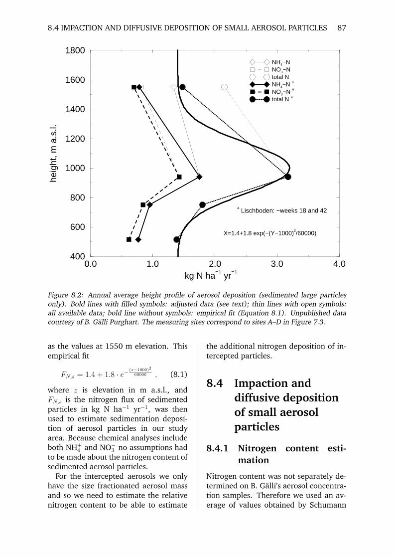
8.4 IMPACTION AND DIFFUSIVE DEPOSITION OF SMALL AEROSOL PARTICLES 87
0.0 1.0 2.0 3.0 4.0kg N ha
−1 yr
−1
400
600
800
1000
1200
1400
1600
1800he
ight
, m a
.s.l.
NH4−N NO3−N total N NH4−N a
NO3−N a
total N a
X=1.4+1.8 exp(−(Y−1000)2/60000)
a Lischboden: −weeks 18 and 42
Figure 8.2: Annual average height profile of aerosol deposition (sedimented large particlesonly). Bold lines with filled symbols: adjusted data (see text); thin lines with open symbols:all available data; bold line without symbols: empirical fit (Equation 8.1). Unpublished datacourtesy of B. Galli Purghart. The measuring sites correspond to sites A–D in Figure 7.3.
as the values at 1550 m elevation. Thisempirical fit
FN,s = 1.4 + 1.8 · e−(z−1000)2
60000 , (8.1)
where z is elevation in m a.s.l., andFN,s is the nitrogen flux of sedimentedparticles in kg N ha−1 yr−1, was thenused to estimate sedimentation deposi-tion of aerosol particles in our studyarea. Because chemical analyses includeboth NH+
4 and NO−3 no assumptions had
to be made about the nitrogen content ofsedimented aerosol particles.
For the intercepted aerosols we onlyhave the size fractionated aerosol massand so we need to estimate the relativenitrogen content to be able to estimate
the additional nitrogen deposition of in-tercepted particles.
8.4 Impaction anddiffusive depositionof small aerosolparticles
8.4.1 Nitrogen content esti-mation
Nitrogen content was not separately de-termined on B. Galli’s aerosol concentra-tion samples. Therefore we used an av-erage of values obtained by Schumann

88 8. DRY DEPOSITION OF AEROSOL PARTICLES
1 2 3 4 5 6 7 8impactor size fraction
0
2
4
6
8
10
12
14ni
trog
en c
onte
nt, %
averageHeimgartner #1Heimgartner #2Heimgartner #3Schumann
1 2 3 4 5 6 7 8impactor size fraction
0
2
4
6
8
10
NH4
+
NO3
-
Figure 8.3: Nitrogen content (mass fraction) of aerosol particles collected on 8 impactor stages:1=0.06–0.125 µm; 2=0.125–0.25 µm; 3=0.25–0.5 µm; 4=0.5–1 µm; 5=1–2 µm; 6=2–4 µm;7=4–8 µm; 8=8–16 µm. Data were taken from Heimgartner 1987 (3 individual measurements)and Schumann 1989. The Schumann data were weighted with factor 3 for the average curve.
(1989) and Heimgartner (1987). Weweighted the published values of Schu-mann (1989) by a factor of 3 whenaveraging them together with the un-published values of Heimgartner (1987).Both data sources show that relative ni-trogen content is largest at intermediateparticle sizes (Figure 8.3) in the range0.25–1.0 µm (impactor stages 3–4), andthat nitrogen content is relatively low forlarge aerosol particles.
For smaller particles the fraction ofNH+
4 nitrogen is higher than the frac-tion of NO−
3 nitrogen, while large parti-cles (stages 7 and 8) contain almost noNH+
4 and NO−3 nitrogen (0.9–1.6%). As
an overall average the thus derived rela-tive nitrogen content of aerosol particlesis 13.3% of total aerosol mass (stages 1–7; 13.0% if stage 8 is included in averag-ing).
The total nitrogen concentration at thefour stations Belpmoos, Hofmatt, Uecht
0.1 1 10particle diameter, µm
0.0
0.5
1.0
1.5
2.0
2.5
µg N
m−
3
Belpmoos 515 m a.s.l.Hofmatt 750 m a.s.l.Uecht 940 m a.s.l.Lischboden 1550 m a.s.l.
Figure 8.4: Size-fractionated concentrationof nitrogen in aerosol particles in a heightprofile near Bern. Data from Galli Purghart(1989), 8 October 1985 to 16 September1986.
and Lischboden on particles <8 µm isthus estimated to be 4.77, 4.01, 3.23,and 1.60 µg N m−3 respectively. Forcomparison we show the bulk concen-tration measurements made at Payerneduring the years 1993 and 1995 (Krieg,
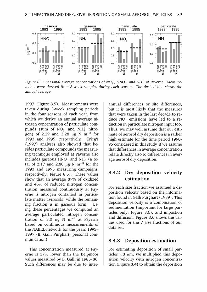
8.4 IMPACTION AND DIFFUSIVE DEPOSITION OF SMALL AEROSOL PARTICLES 89
Win
ter
Spr
ing
Sum
mer
Fal
l
Win
ter
Spr
ing
Sum
mer
Fal
l 0.0
0.1
0.2
0.3
µg m
−3
gaseous1993 1995
Win
ter
Spr
ing
Sum
mer
Fal
l
Win
ter
Spr
ing
Sum
mer
Fal
l
0.0
1.0
2.0
3.0
4.0
gaseous1993 1995
Win
ter
Spr
ing
Sum
mer
Fal
l
Win
ter
Spr
ing
Sum
mer
Fal
l
0.0
0.5
1.0
1.5
2.0
particulate1993 1995
Win
ter
Spr
ing
Sum
mer
Fal
l
Win
ter
Spr
ing
Sum
mer
Fal
l
0.0
1.0
2.0
3.0
particulate1993 1995
HNO3NH3 NO3
− NH4
+
Figure 8.5: Seasonal average concentrations of NO−3 , HNO3, and NH+
4 at Payerne. Measure-ments were derived from 3-week samples during each season. The dashed line shows theannual average.
1997; Figure 8.5). Measurements weretaken during 3-week sampling periodsin the four seasons of each year, fromwhich we derive an annual average ni-trogen concentration of particulate com-punds (sum of NO−
3 and NH+4 nitro-
gen) of 2.29 and 3.28 µg N m−3 for1993 and 1995, respectively. Krieg‘s(1997) analyses also showed that be-sides particulate compounds the measur-ing technique employed at Payerne alsoincludes gaseous HNO3 and NH3 (a to-tal of 2.17 and 2.80 µg N m−3 for the1993 and 1995 measuring campaigns,respectively; Figure 8.5). These valuesshow that an average 87% of oxidizedand 46% of reduced nitrogen concen-tration measured continuously at Pay-erne is nitrogen contained in particu-late matter (aerosols) while the remain-ing fraction is in gaseous form. Us-ing these percentages we computed anaverage particulated nitrogen concen-tration of 3.0 µg N m−3 at Payernebased on continuous measurements ofthe NABEL-network for the years 1993–1997 (B. Galli Purghart, personal com-munication).
This concentration measured at Pay-erne is 37% lower than the Belpmoosvalues measured by B. Galli in 1985/86.Such differences may be due to inter-
annual differences or site differences,but it is most likely that the measuresthat were taken in the last decade to re-duce NOx emissions have led to a re-duction in particulate nitrogen input too.Thus, we may well assume that our esti-mate of aerosol dry deposition is a ratherhigh estimate for the time period 1990-95 considered in this study, if we assumethat differences in average concentrationrelate directly also to differences in aver-age aerosol dry deposition.
8.4.2 Dry deposition velocityestimation
For each size fraction we assumed a de-position velocity based on the informa-tion found in Galli Purghart (1989). Thisdeposition velocity is a combination ofsedimentation (important for large par-ticles only; Figure 8.6), and impactionand diffusion. Figure 8.6 shows the val-ues used for the 7 size fractions of ourdata set.
8.4.3 Deposition estimation
For estimating deposition of small par-ticles <8 µm, we multiplied this depo-sition velocity with nitrogen concentra-tion (Figure 8.4) to obtain the deposition
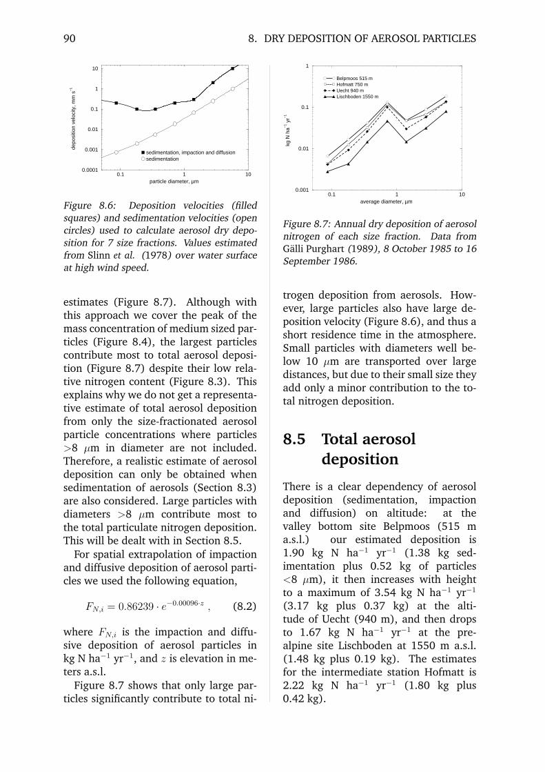
90 8. DRY DEPOSITION OF AEROSOL PARTICLES
0.1 1 10particle diameter, µm
0.0001
0.001
0.01
0.1
1
10de
posi
tion
velo
city
, mm
s−
1
sedimentation, impaction and diffusionsedimentation
Figure 8.6: Deposition velocities (filledsquares) and sedimentation velocities (opencircles) used to calculate aerosol dry depo-sition for 7 size fractions. Values estimatedfrom Slinn et al. (1978) over water surfaceat high wind speed.
estimates (Figure 8.7). Although withthis approach we cover the peak of themass concentration of medium sized par-ticles (Figure 8.4), the largest particlescontribute most to total aerosol deposi-tion (Figure 8.7) despite their low rela-tive nitrogen content (Figure 8.3). Thisexplains why we do not get a representa-tive estimate of total aerosol depositionfrom only the size-fractionated aerosolparticle concentrations where particles>8 µm in diameter are not included.Therefore, a realistic estimate of aerosoldeposition can only be obtained whensedimentation of aerosols (Section 8.3)are also considered. Large particles withdiameters >8 µm contribute most tothe total particulate nitrogen deposition.This will be dealt with in Section 8.5.
For spatial extrapolation of impactionand diffusive deposition of aerosol parti-cles we used the following equation,
FN,i = 0.86239 · e−0.00096·z , (8.2)
where FN,i is the impaction and diffu-sive deposition of aerosol particles inkg N ha−1 yr−1, and z is elevation in me-ters a.s.l.
Figure 8.7 shows that only large par-ticles significantly contribute to total ni-
0.1 1 10average diameter, µm
0.001
0.01
0.1
1
kg N
ha−
1 yr−
1
Belpmoos 515 mHofmatt 750 mUecht 940 mLischboden 1550 m
Figure 8.7: Annual dry deposition of aerosolnitrogen of each size fraction. Data fromGalli Purghart (1989), 8 October 1985 to 16September 1986.
trogen deposition from aerosols. How-ever, large particles also have large de-position velocity (Figure 8.6), and thus ashort residence time in the atmosphere.Small particles with diameters well be-low 10 µm are transported over largedistances, but due to their small size theyadd only a minor contribution to the to-tal nitrogen deposition.
8.5 Total aerosoldeposition
There is a clear dependency of aerosoldeposition (sedimentation, impactionand diffusion) on altitude: at thevalley bottom site Belpmoos (515 ma.s.l.) our estimated deposition is1.90 kg N ha−1 yr−1 (1.38 kg sed-imentation plus 0.52 kg of particles<8 µm), it then increases with heightto a maximum of 3.54 kg N ha−1 yr−1
(3.17 kg plus 0.37 kg) at the alti-tude of Uecht (940 m), and then dropsto 1.67 kg N ha−1 yr−1 at the pre-alpine site Lischboden at 1550 m a.s.l.(1.48 kg plus 0.19 kg). The estimatesfor the intermediate station Hofmatt is2.22 kg N ha−1 yr−1 (1.80 kg plus0.42 kg).
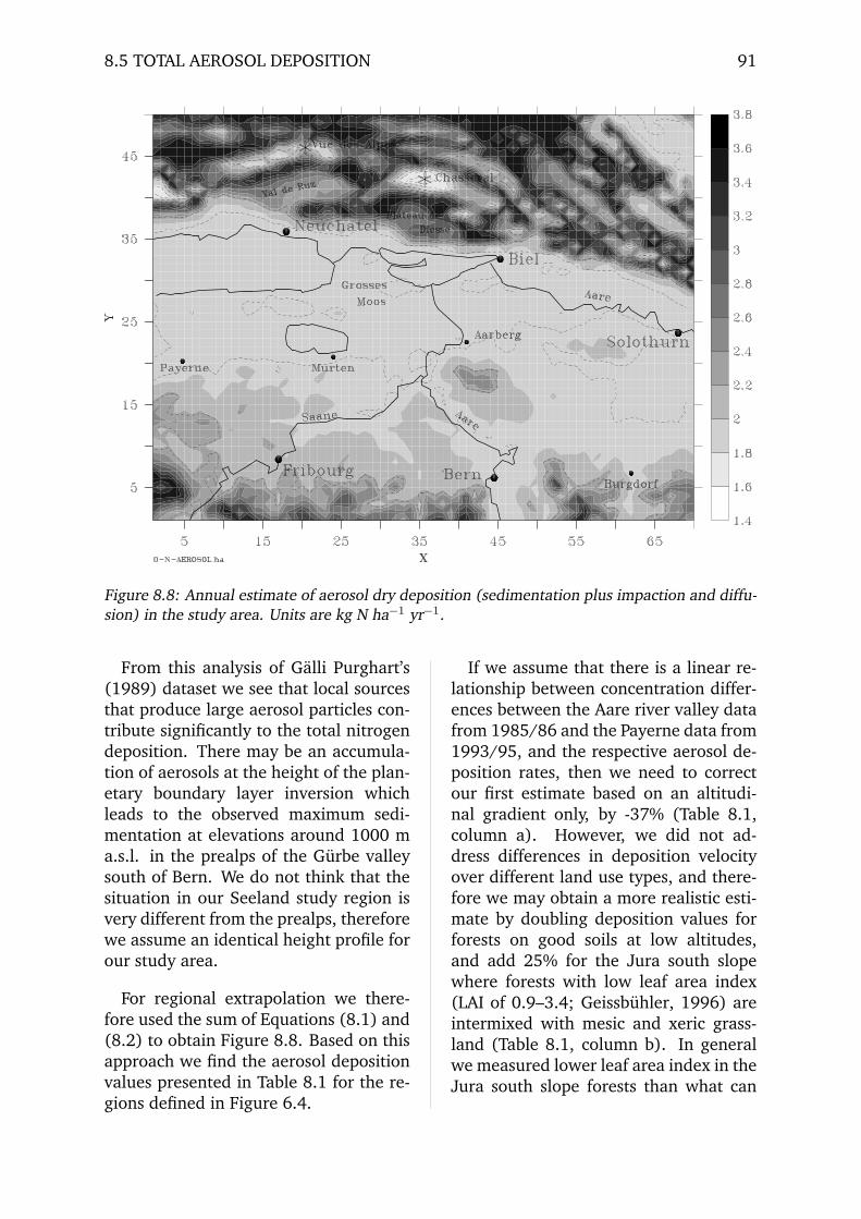
8.5 TOTAL AEROSOL DEPOSITION 91
Figure 8.8: Annual estimate of aerosol dry deposition (sedimentation plus impaction and diffu-sion) in the study area. Units are kg N ha−1 yr−1.
From this analysis of Galli Purghart’s(1989) dataset we see that local sourcesthat produce large aerosol particles con-tribute significantly to the total nitrogendeposition. There may be an accumula-tion of aerosols at the height of the plan-etary boundary layer inversion whichleads to the observed maximum sedi-mentation at elevations around 1000 ma.s.l. in the prealps of the Gurbe valleysouth of Bern. We do not think that thesituation in our Seeland study region isvery different from the prealps, thereforewe assume an identical height profile forour study area.
For regional extrapolation we there-fore used the sum of Equations (8.1) and(8.2) to obtain Figure 8.8. Based on thisapproach we find the aerosol depositionvalues presented in Table 8.1 for the re-gions defined in Figure 6.4.
If we assume that there is a linear re-lationship between concentration differ-ences between the Aare river valley datafrom 1985/86 and the Payerne data from1993/95, and the respective aerosol de-position rates, then we need to correctour first estimate based on an altitudi-nal gradient only, by -37% (Table 8.1,column a). However, we did not ad-dress differences in deposition velocityover different land use types, and there-fore we may obtain a more realistic esti-mate by doubling deposition values forforests on good soils at low altitudes,and add 25% for the Jura south slopewhere forests with low leaf area index(LAI of 0.9–3.4; Geissbuhler, 1996) areintermixed with mesic and xeric grass-land (Table 8.1, column b). In generalwe measured lower leaf area index in theJura south slope forests than what can
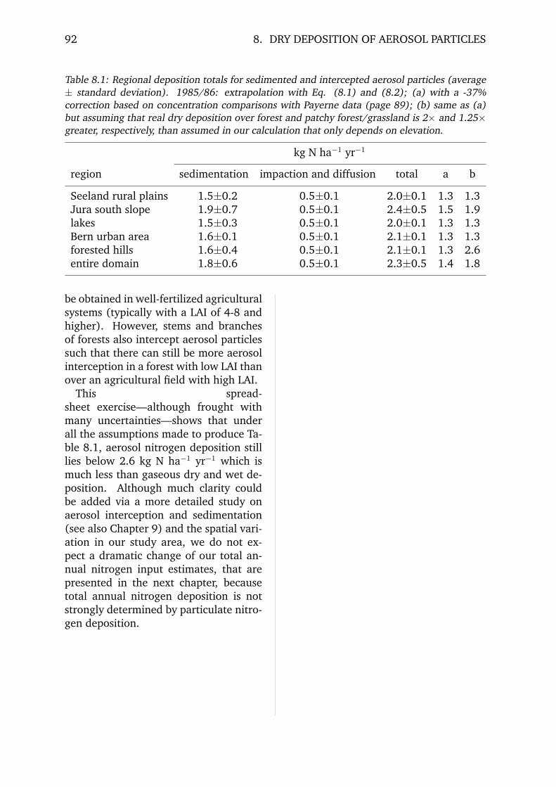
92 8. DRY DEPOSITION OF AEROSOL PARTICLES
Table 8.1: Regional deposition totals for sedimented and intercepted aerosol particles (average± standard deviation). 1985/86: extrapolation with Eq. (8.1) and (8.2); (a) with a -37%correction based on concentration comparisons with Payerne data (page 89); (b) same as (a)but assuming that real dry deposition over forest and patchy forest/grassland is 2× and 1.25×greater, respectively, than assumed in our calculation that only depends on elevation.
kg N ha−1 yr−1
region sedimentation impaction and diffusion total a b
Seeland rural plains 1.5±0.2 0.5±0.1 2.0±0.1 1.3 1.3Jura south slope 1.9±0.7 0.5±0.1 2.4±0.5 1.5 1.9lakes 1.5±0.3 0.5±0.1 2.0±0.1 1.3 1.3Bern urban area 1.6±0.1 0.5±0.1 2.1±0.1 1.3 1.3forested hills 1.6±0.4 0.5±0.1 2.1±0.1 1.3 2.6entire domain 1.8±0.6 0.5±0.1 2.3±0.5 1.4 1.8
be obtained in well-fertilized agriculturalsystems (typically with a LAI of 4-8 andhigher). However, stems and branchesof forests also intercept aerosol particlessuch that there can still be more aerosolinterception in a forest with low LAI thanover an agricultural field with high LAI.
This spread-sheet exercise—although frought withmany uncertainties—shows that underall the assumptions made to produce Ta-ble 8.1, aerosol nitrogen deposition stilllies below 2.6 kg N ha−1 yr−1 which ismuch less than gaseous dry and wet de-position. Although much clarity couldbe added via a more detailed study onaerosol interception and sedimentation(see also Chapter 9) and the spatial vari-ation in our study area, we do not ex-pect a dramatic change of our total an-nual nitrogen input estimates, that arepresented in the next chapter, becausetotal annual nitrogen deposition is notstrongly determined by particulate nitro-gen deposition.

9. Comparison with Swiss Study andOpen Questions
9.1 Differences betweenthis study and Rihm(1996)
The modeling concept of the earlierRihm (1996) study is very different fromthe present study. Therefore, a detailedcomparison of the model results of bothstudies was made to assess potentialproblems and uncertainties that may ex-ist with either of the two modeling ap-proaches.
The advantage of the approach usedby Rihm (1996), which employs a ge-ographical information system (GIS), is(a) the ability to cover the whole ofSwitzerland at the 1 km2 resolution,and (b) the possibility for quick up-dates when the emission inventorieschange. The disadvantage is, however,that only statistical extrapolation meth-ods are used which do not consider ac-tual weather conditions, such as pre-vailing wind direction, atmospheric sta-bility, or wind speed. In particular,Rihm (1996) used constant land-use spe-cific deposition velocities for estimatinggaseous dry deposition.
The advantage of the approach usedby Metphomod is that many physicalprocesses are modeled in a mechanisticway that allows incorporation of actualweather conditions and turbulent trans-port mechanisms. The disadvantage isthe smaller domain size and the highcomplexity of the model which makes itmore difficult to interpret the results.
Both model approaches rely on similarinput data (emission inventories) which,however, are subject to development andchanges. For example, Reinhardt (1995)obtained 28.7% greater ammonia emis-sions in 1994/1995 with his seasonalmethod (Section 5.3.1) than with theemission factor method. However, forthe present comparison with the Rihm(1996) GIS model, the newest versionof the ammonia emission inventory wasalso used. Interestingly, the findingsby Reinhardt (1995) are now incorpo-rated in the most current emission fac-tors, which even exceed the values pro-posed by Reinhardt in 1995. For ex-ample, over the Seeland domain consid-ered in this report, the most recent am-monia emission inventory produces 18%greater annual emissions than the inven-tory used for this study.
On the other hand, a decrease in theemission and concentration of oxidizednitrogen compounds has been observedover the past 10 years in Switzerland(Filliger, 1998). NOx concentration de-creased by 37%, NO2 by 28% (Filliger,1998). As of June 1998, the newestemission inventory used with the Rihm(1996) GIS model yields 8,429 tonnesof total N deposition per year over theSeeland domain (corresponding to 24.0kg N ha−1 yr−1) while the total annualnitrogen deposition computed with theMetphomod model approach employedin this study is 8,625 tonnes N yr−1 or24.6 kg N ha−1 yr−1.
This small difference is acceptable,
93
94 9. COMPARISON WITH SWISS STUDY AND OPEN QUESTIONS
but it appears that with the newer in-put data the ratio between the depo-sitions of reduced nitrogen compounds(NHx), and of oxidized nitrogen com-pounds (NOx) would shift more towardsincreasing NHx depositions, while NOx
depositions would be slightly decreas-ing. However, both approaches agreein their general finding that the deposi-tion amounts of reduced nitrogen com-pounds are the dominant input in all ar-eas except in the centers of cities (espe-cially in Bern), were NOx deposition isthe dominant form of nitrogen deposi-tion.
The deposition amounts actually re-ceived by different land-use types varymore strongly between the two modelapproaches. While the GIS model doesnot take into account any dynamic ef-fects of accumulation behind obstacles(hills, mountain ranges) there is muchmore small-scale variation in the Met-phomod results. The GIS model usesan inverse distance method for estimat-ing deposition fluxes as a function ofthe distance from the source. No site-specific wind patterns are incorporatedin this extrapolation method, and the lat-eral dispersion of trace gases in the See-land is overestimated. The annual de-position totals of individual 1 km2 gridcells along the Jura south slope typi-cally agree within ±5–10 kg N ha−1 yr−1,while the GIS estimates for the south-eastern part of the model domain exhibita high bias compared with the Metpho-mod approach, particularly over forests.
One problem that emerged in thiscomparison and which may also be im-portant for interpreting these differencesis the following: the GIS approach used alattice system where the nodes of a meshwith 1 km2 spacing are modeled, whileMetphomod results express averages ofthe 1 km2 grid cells. Therefore, the land-use class of a GIS lattice node may differfrom the dominant or effective land use
defined for the corresponding grid cell inMetphomod.
The Metphomod annual depositionamounts for lakes and the urban areaof Bern are significantly higher than theGIS results, which tend to underestimatethe nitrogen deposition for individualgrid cells.
9.2 Open Questions
9.2.1 Ammonia Deposition toOpen Water
The problem of estimating ammonia de-position to open water surfaces has beenbrought to our attention by one of thereferees who reviewed the scientific ar-ticle by Eugster et al. (1998). Olderstudies rely on the fact that ammoniais easily soluble in water with a pH be-low 7–8, and therefore it was assumedin this study that there is no uptake re-sistance Rc for ammonia, such that de-position of ammonia to an open watersurface is only determined by the atmo-spheric and boundary-layer resistancesRa + Rb. This assumption is now un-der debate due to recent publicationswhich show that there might still be aconsiderable uptake resistance for am-monia even when the water pH is be-low 7–8. Because it was never the in-tention of this project to assess the nitro-gen inputs to the lakes in particular, it isonly stated here that the deposition val-ues to lake surfaces—which also differstrongly between the GIS approach andMetphomod—may be subject to signifi-cant changes if this model study shouldbe replicated. It is suggested to per-form laboratory experiments with sur-face water samples taken from the lakesof Neuchatel, Biel and Murten, in orderto directly determine Rc. This estimatewould then be less uncertain than the lit-erature values employed in this study.
9.2 OPEN QUESTIONS 95
9.2.2 Occult Deposition
Another open question is the occult de-position inputs during fog events, whichare not currently included in our annualestimates. It is expected that occult de-position to the montane and subalpineforests may add as much as 30–40% tothe annual wet deposition. It is currentlynot possible to make credible estimatesof occult deposition inputs in the See-land study area. However, because ofthe known high frequency of winter fogevents, it is very likely that future de-velopments in this research area will in-crease annual estimates of nitrogen de-position considerably when occult depo-sition is included.
9.2.3 Conversion of Ammoniato Ammonium
The version of Metphomod used inthis study does not consider heteroge-neous reactions of ammonia to formammonium-containing aerosol particles.Therefore, in the present approach,the dry deposition of particulate mat-ter was treated independently from thegaseous dry deposition. However, theresidence time of gaseous ammonia ismuch shorter than that for ammoniumin aerosol particles. Thus, local depo-sition of ammonia may be overempha-sised in the present approach because lo-cally emitted ammonia is not convertedto ammonium and therefore can not betransported over large distances. In theGIS approach the ratio between locallydeposited and locally emitted ammoniais prescribed to be 46%, while a ratio of57% is obtained via the Metphomod ap-proach. Although only a small fraction ofgaseous ammonia is in fact converted toaerosols and then transported over largedistances, this mechanism may be impor-tant in rural areas where reduced nitro-gen compounds dominate annual depo-
sition totals.
9.2.4 The Role of Oxidation ofNOx to HNO3
Metphomod results for oxidized nitro-gen compounds exhibit a relatively smallcontribution of HNO3 deposition to theNOy deposition total (typically less than10%). Long-term field measurements atthe Harvard Forest research site in NorthAmerica, however, suggest that oxida-tion of NO2 to HNO3 in the presence ofozone and aerosol particles is importantfor NOy deposition budgets (Mungeret al., 1998). The chemistry module ofMetphomod includes oxidation of NO2
to NO3 in the presence of O3 and the sub-sequent reaction NO3+NO2 →N2O5, butit does not include the heterogeneous re-action N2O5+H2O→HNO3 in the pres-ence of aerosols (Munger et al., 1998).Therefore, the HNO3 concentrations anddeposition fluxes in Metphomod compu-tations may be significantly lower thanthey would be if heterogeneous chemi-cal reactions were already included. Thisimplies that inclusion of heterogeneouschemical reactions in future versions ofMetphomod’s chemistry module may in-crease the significance of oxidized nitro-gen deposition in the study area com-pared with the current estimates for thisreport.
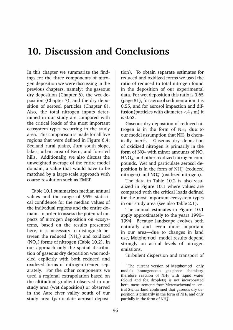
10. Discussion and Conclusions
In this chapter we summarize the find-ings for the three components of nitro-gen deposition we were discussing in theprevious chapters, namely: the gaseousdry deposition (Chapter 6), the wet de-position (Chapter 7), and the dry depo-sition of aerosol particles (Chapter 8).Also, the total nitrogen inputs deter-mined in our study are compared withthe critical loads of the most importantecosystem types occurring in the studyarea. This comparison is made for all fiveregions that were defined in Figure 6.4:Seeland rural plains, Jura south slope,lakes, urban area of Bern, and forestedhills. Additionally, we also discuss theunweighted average of the entire modeldomain, a value that would have to bematched by a large-scale approach withcoarse resolution such as EMEP.
Table 10.1 summarizes median annualvalues and the range of 95% statisti-cal confidence for the median values ofthe individual regions and the entire do-main. In order to assess the potential im-pacts of nitrogen deposition on ecosys-tems, based on the results presentedhere, it is necessary to distinguish be-tween the reduced (NHx) and oxidized(NOy) forms of nitrogen (Table 10.2). Inour approach only the spatial distribu-tion of gaseous dry deposition was mod-eled explicitly with both reduced andoxidized forms of nitrogen treated sep-arately. For the other components weused a regional extrapolation based onthe altitudinal gradient observed in ourstudy area (wet deposition) or observedin the Aare river valley south of ourstudy area (particulate aerosol deposi-
tion). To obtain separate estimates forreduced and oxidized forms we used theratio of reduced to total nitrogen foundin the deposition of our experimentaldata. For wet deposition this ratio is 0.65(page 81), for aerosol sedimentation it is0.55, and for aerosol impaction and dif-fusion(particles with diameter <4 µm) itis 0.63.
Gaseous dry deposition of reduced ni-trogen is in the form of NH3 due toour model assumption that NH3 is chem-ically inert1. Gaseous dry depositionof oxidized nitrogen is primarily in theform of NO2 with minor amounts of NO,HNO3, and other oxidized nitrogen com-pounds. Wet and particulate aerosol de-position is in the form of NH+
4 (reducednitrogen) and NO−
3 (oxidized nitrogen).The data in Table 10.2 is also visu-
alized in Figure 10.1 where values arecompared with the critical loads definedfor the most important ecosystem typesin our study area (see also Table 2.1).
The annual estimates in Figure 10.1apply approximately to the years 1990–1994. Because landscape evolves bothnaturally and—even more importantin our area—due to changes in landuse, Metphomod model results dependstrongly on actual levels of nitrogenemissions.
Turbulent dispersion and transport of
1The current version of Metphomod onlymodels homogeneous gas-phase chemistry,therefore reaction of NH3 with liquid water(cloud and fog droplets) is not incorporatedhere; measurements from Merenschwand in cen-tral Switzerland confirmed that gaseous dry de-position is primarily in the form of NH3 and onlypartially in the form of NH+
4 .
96
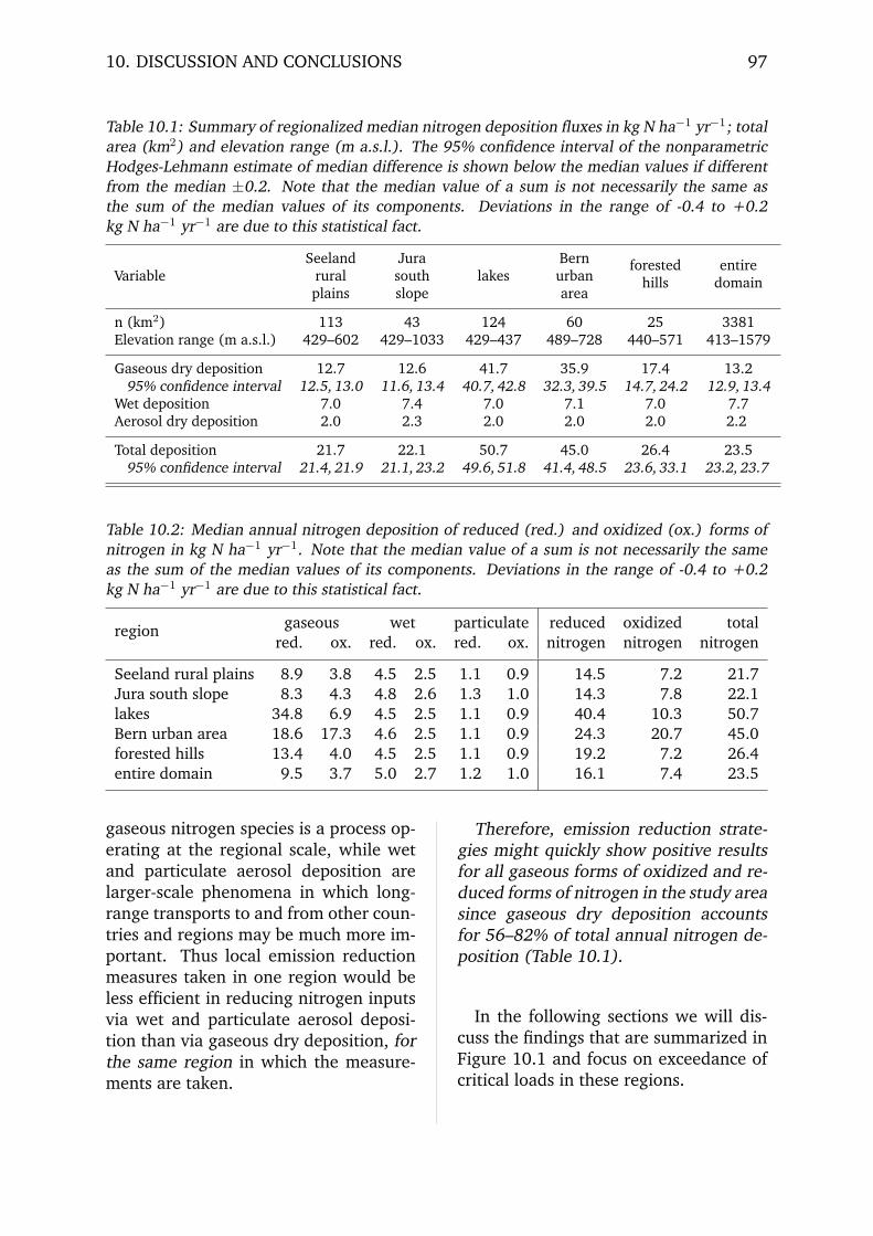
10. DISCUSSION AND CONCLUSIONS 97
Table 10.1: Summary of regionalized median nitrogen deposition fluxes in kg N ha−1 yr−1; totalarea (km2) and elevation range (m a.s.l.). The 95% confidence interval of the nonparametricHodges-Lehmann estimate of median difference is shown below the median values if differentfrom the median ±0.2. Note that the median value of a sum is not necessarily the same asthe sum of the median values of its components. Deviations in the range of -0.4 to +0.2kg N ha−1 yr−1 are due to this statistical fact.
Seeland Jura BernVariable rural south lakes urban
forested entire
plains slope areahills domain
n (km2) 113 43 124 60 25 3381Elevation range (m a.s.l.) 429–602 429–1033 429–437 489–728 440–571 413–1579
Gaseous dry deposition 12.7 12.6 41.7 35.9 17.4 13.295% confidence interval 12.5, 13.0 11.6, 13.4 40.7, 42.8 32.3, 39.5 14.7, 24.2 12.9, 13.4
Wet deposition 7.0 7.4 7.0 7.1 7.0 7.7Aerosol dry deposition 2.0 2.3 2.0 2.0 2.0 2.2
Total deposition 21.7 22.1 50.7 45.0 26.4 23.595% confidence interval 21.4, 21.9 21.1, 23.2 49.6, 51.8 41.4, 48.5 23.6, 33.1 23.2, 23.7
Table 10.2: Median annual nitrogen deposition of reduced (red.) and oxidized (ox.) forms ofnitrogen in kg N ha−1 yr−1. Note that the median value of a sum is not necessarily the sameas the sum of the median values of its components. Deviations in the range of -0.4 to +0.2kg N ha−1 yr−1 are due to this statistical fact.
gaseous wet particulate reduced oxidized totalregionred. ox. red. ox. red. ox. nitrogen nitrogen nitrogen
Seeland rural plains 8.9 3.8 4.5 2.5 1.1 0.9 14.5 7.2 21.7Jura south slope 8.3 4.3 4.8 2.6 1.3 1.0 14.3 7.8 22.1lakes 34.8 6.9 4.5 2.5 1.1 0.9 40.4 10.3 50.7Bern urban area 18.6 17.3 4.6 2.5 1.1 0.9 24.3 20.7 45.0forested hills 13.4 4.0 4.5 2.5 1.1 0.9 19.2 7.2 26.4entire domain 9.5 3.7 5.0 2.7 1.2 1.0 16.1 7.4 23.5
gaseous nitrogen species is a process op-erating at the regional scale, while wetand particulate aerosol deposition arelarger-scale phenomena in which long-range transports to and from other coun-tries and regions may be much more im-portant. Thus local emission reductionmeasures taken in one region would beless efficient in reducing nitrogen inputsvia wet and particulate aerosol deposi-tion than via gaseous dry deposition, forthe same region in which the measure-ments are taken.
Therefore, emission reduction strate-gies might quickly show positive resultsfor all gaseous forms of oxidized and re-duced forms of nitrogen in the study areasince gaseous dry deposition accountsfor 56–82% of total annual nitrogen de-position (Table 10.1).
In the following sections we will dis-cuss the findings that are summarized inFigure 10.1 and focus on exceedance ofcritical loads in these regions.
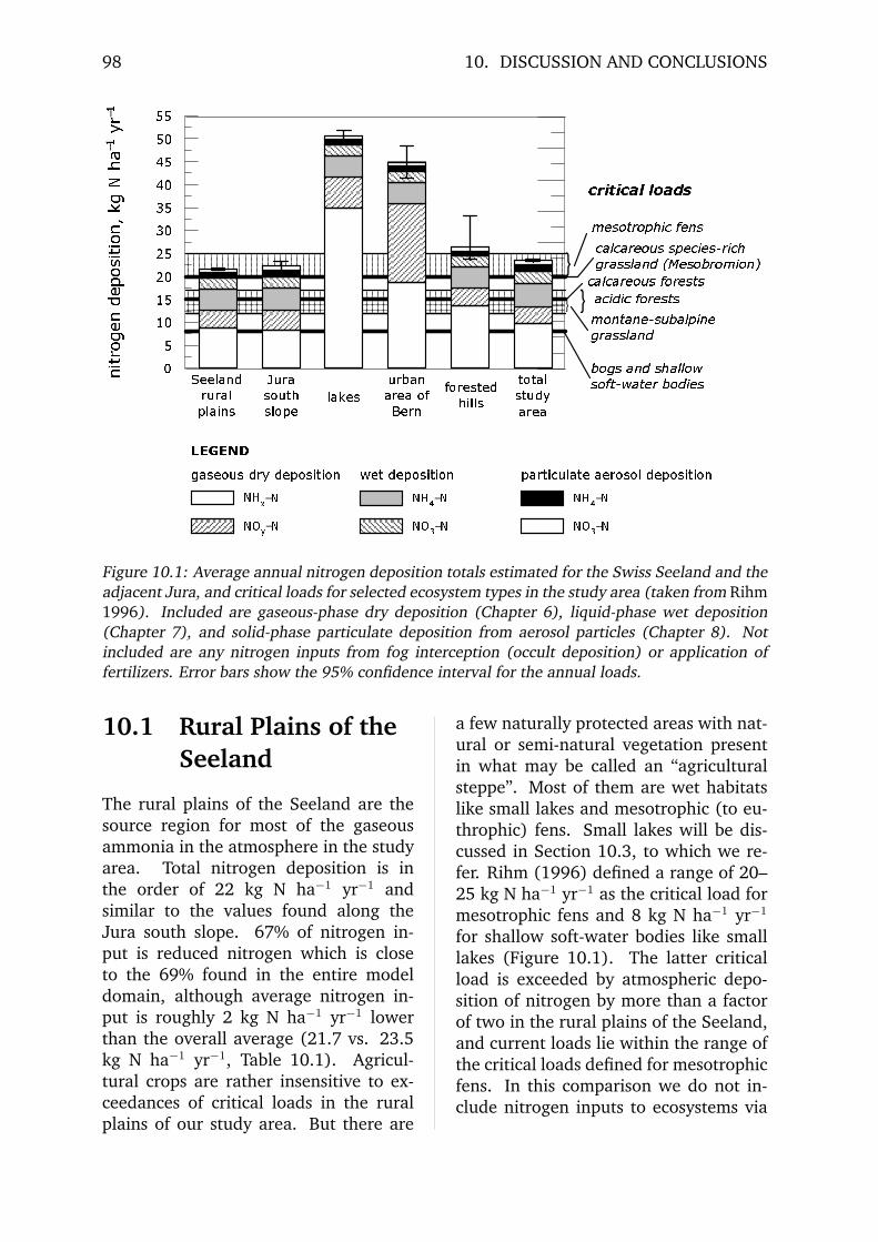
98 10. DISCUSSION AND CONCLUSIONS
��
��������������������
QLWURJH
Q�GHS
RVLWLR
Q��NJ
�1�KD
���\U
��
-XUDVRXWKVORSH
ODNHV6HHODQGUXUDOSODLQV
XUEDQDUHD�RI%HUQ
IRUHVWHGKLOOV
WRWDOVWXG\DUHD
}
}}
PHVRWURSKLF�IHQV
DFLGLF�IRUHVWVPRQWDQH�VXEDOSLQHJUDVVODQG
ERJV�DQG�VKDOORZVRIW�ZDWHU�ERGLHV
FDOFDUHRXV�IRUHVWV
FDOFDUHRXV�VSHFLHV�ULFKJUDVVODQG��0HVREURPLRQ�
FULWLFDO�ORDGV
1+[�112\�1
1+��112��1
1+��112��1
JDVHRXV�GU\�GHSRVLWLRQ ZHW�GHSRVLWLRQ SDUWLFXODWH�DHURVRO�GHSRVLWLRQ/(*(1'
Figure 10.1: Average annual nitrogen deposition totals estimated for the Swiss Seeland and theadjacent Jura, and critical loads for selected ecosystem types in the study area (taken from Rihm1996). Included are gaseous-phase dry deposition (Chapter 6), liquid-phase wet deposition(Chapter 7), and solid-phase particulate deposition from aerosol particles (Chapter 8). Notincluded are any nitrogen inputs from fog interception (occult deposition) or application offertilizers. Error bars show the 95% confidence interval for the annual loads.
10.1 Rural Plains of theSeeland
The rural plains of the Seeland are thesource region for most of the gaseousammonia in the atmosphere in the studyarea. Total nitrogen deposition is inthe order of 22 kg N ha−1 yr−1 andsimilar to the values found along theJura south slope. 67% of nitrogen in-put is reduced nitrogen which is closeto the 69% found in the entire modeldomain, although average nitrogen in-put is roughly 2 kg N ha−1 yr−1 lowerthan the overall average (21.7 vs. 23.5kg N ha−1 yr−1, Table 10.1). Agricul-tural crops are rather insensitive to ex-ceedances of critical loads in the ruralplains of our study area. But there are
a few naturally protected areas with nat-ural or semi-natural vegetation presentin what may be called an “agriculturalsteppe”. Most of them are wet habitatslike small lakes and mesotrophic (to eu-throphic) fens. Small lakes will be dis-cussed in Section 10.3, to which we re-fer. Rihm (1996) defined a range of 20–25 kg N ha−1 yr−1 as the critical load formesotrophic fens and 8 kg N ha−1 yr−1
for shallow soft-water bodies like smalllakes (Figure 10.1). The latter criticalload is exceeded by atmospheric depo-sition of nitrogen by more than a factorof two in the rural plains of the Seeland,and current loads lie within the range ofthe critical loads defined for mesotrophicfens. In this comparison we do not in-clude nitrogen inputs to ecosystems via

10.2 THE LOWER JURA SOUTH SLOPE 99
the leaching of dissolved nitrate fromclose-by agricultural fields (that con-tribute further to euthrophication). It isvery likely that the combination of atmo-spheric and hydrospheric nitrogen loadssignificantly exceeds the critical loadsfor mesotrophic fens, whilst atmosphericinputs alone only exceed critical loadsfor nitrogen-poor ecosystems (bogs andshallow soft-water bodies), and decidu-ous and coniferous forests on acidic soils(critical load of 12–17 kg N ha−1 yr−1).
10.2 The Lower JuraSouth Slope
Our estimated annual total of nitrogendeposition to the lower elevations of theJura south slope is 22.1 kg nitrogen perhectar. This number does not include thelargely unknown contribution of fog in-terception (occult deposition) that mightbe important along the Jura south slope(see Chapter 9). However, even thepresent estimate is significantly abovethe critical load for calcareous forests(15 kg N ha−1 yr−1) and the critical loadof managed species-rich grassland oncalcareous ground (e.g. Mesobromion,20 kg N ha−1 yr−1, Figure 10.1).
The pubescent oak forests (Quercionpubescentis) that were the focus ofGeissbuhler’s (1996) contribution to thisstudy are the most important nutrient-poor forest ecosystem type along theJura south slope at lower elevations.They receive an annual nitrogen inputof at least 22.1 kg of nitrogen per hec-tar (fog interception not included) whichis roughly 7 kg or 48% above the valuerecommended by Rihm (1996). Thecritical load for an ecosystem was esti-mated by Rihm (1996) in a complex pro-cedure that not only looks at absolutenitrogen input, but places this in rela-tion to denitrification rate, leaching rate,and nitrogen immobilization rate, from
which the effective nitrogen available forplant growth can be derived (Posch et al.,1995). Thus, they represent best avail-able knowledge. Via the work done byGeissbuhler (1996) we made sure of ob-taining reasonable results for this ecosys-tem type even though it is not the mostwide-spread. Therefore, there is 95%confidence that the current nitrogen in-put to pubescent oak forests along theJura south slope is actually exceedingboth the recommended critical load forthis ecosystem type, as well as the up-per bound of the range given in Table 2.1which is exceeded by 2.1 kg N ha−1 yr−1
or 11%.So far, we have not addressed the
situation of the higher elevations ofthe Jura south slope since the domi-nant vegetation type there is fir forestintermixed with some deciduous trees(maple, beech). This type of coniferousforest on nonacidic surface is less suscep-tible to atmospheric nitrogen inputs thanthe ecosystem types found at lower ele-vations, and therefore we do not expect asignificant exceedance of the critical loadat higher elevations. Because elevationsgreater than 1000–1200 m a.s.l. are gen-erally above the typical winter fog layerin this area, we also do not expect a sig-nificant nitrogen input by fog intercep-tion that was neglected in this study dueto unavailability of representative datafor the area of interest.
An interesting point in the compari-son with the adjacent lakes (discussed inthe next section) is the abrupt change inrelative contribution of gaseous ammo-nia between lakes and the lower eleva-tions of the Jura south slope. Along theJura south slope 38% of total nitrogendeposition is gaseous dry deposition ofammonia while it is 69% over the lakes.At the beginning of this project we es-tablished a working hypothesis that am-monia emissions from the Seeland ruralplains are transported via the local wind

100 10. DISCUSSION AND CONCLUSIONS
systems towards the Jura south slopewhere there would be a significantly in-creased input of locally emitted ammo-nia from agricultural sources. However,our results show a very different picture:nitrogen input along the Jura south slopeis not significantly higher than over therural plains of the Seeland, and it is verylikely that the lakes act as a filter or bar-rier for ammonia, acting so between thesource region of the Seeland and the re-ceptor region along the Jura south slope.There is strong evidence that the lakesare absorbing most of the locally emittedammonia from agricultural sources.
However, the parameters used for es-timating NH3 deposition over the lakesare currently under dispute as stated inChapter 9.2.1. It is therefore likely thatif deposition of reduced nitrogen is cur-rently overestimated over lakes, then de-position amounts along the lower Jurasouth slope would increase as depositionover lakes decreases.
10.3 Lakes and OtherWater Bodies
Although only large lakes are repre-sented in the Metphomod model, the re-sults also apply to smaller lakes with anextent of less than 1 km2 (the grid reso-lution of Metphomod) and other aquaticsystems like rivers.
The most important finding is thedominance of gaseous ammonia depo-sition that contributes 69% to total an-nual nitrogen deposition. This is a resultof the intensive agricultural land use inthe rural plains of the Seeland and thephysical fact that ammonia is water sol-uble while the oxidized forms of nitro-gen (primarily NO2 and NO) are not. Foraquatic ecosystems the nitrogen inputfrom the atmosphere is not the only in-put pathway for nitrogen, and the well-known nitrate leaching from agricultural
fields may substantially increase currentloads of nitrogen to aquatic ecosystemsby imports from rivers entering a lake.The critical load for shallow soft-waterbodies of 5–10 kg N ha−1 yr−1 (recom-mended value is 8 kg N ha−1 yr−1) is ex-ceeded 6-fold by the current inputs viadeposition from the atmosphere alone.
This raises an open question of howadditional nitrogen input from the atmo-sphere may affect aquatic ecosystems.Based on our model results it does notseem very likely that current nitrogendeposition loads could be reduced belowthe critical load for shallow soft-waterbodies, even under a scenario with zeroagricultural land use (which would elim-inate almost all NHx dry deposition) be-cause the remaining deposition of 15.9kg N ha−1 yr−1 (Table 2.1) is still dou-ble the critical load defined for shallowsoft-water bodies.
The situation, however, may be lessdramatic for the larger lakes such asthe Lake of Neuchatel, the Lake of Bieland the Lake of Murten, where the ra-tio between lake surface and total mixedvolume of the water body (the volumebetween the lake surface and the ther-mocline) is much lower than in shal-low lakes. Because the current prob-lems with dissolved nitrate in the riverand lake water are known and reduc-tion strategies for these nitrogen sourcesare available, there has not so far beena strong focus on the additional at-mospheric inputs of nitrogen to theseecosystems. Our computations, however,show that atmospheric inputs of nitrogento aquatic systems are of an importantand non-negligible quantity.
10.4 The Urban Area ofBern
It is not surprising that an urban areasuch as the one chosen for this study

10.5 FORESTED HILLS IN THE SEELAND 101
has high nitrogen deposition. How-ever, it was a surprise to realize thatthe Metphomod model shows less ni-trogen deposition in the urban area ofBern than what we found over the threelakes in the Seeland (45.0 vs. 50.7kg N ha−1 yr−1). Plate A.4 in the Ap-pendix shows that even within the ur-ban area of Bern there are only a fewhot spots where nitrogen deposition ex-ceeds the values found over the lakes.These locations in the northeast of thecity of Bern are located on the freeway(Tiefenau viaduct and Schonbuhl free-way intersection) where traffic density ishighest. Apart from these two hot spotsthe spatial distribution of nitrogen depo-sition over the urban area of Bern is sim-ilar to the values over the lakes.
An important difference in the com-parison of nitrogen inputs to lakes withthe inputs received in the urban area ofBern is the chemical form of nitrogen de-position. As expected the relative frac-tion of oxidized nitrogen (with traffic, in-dustrial, and residential heating as pri-mary sources) is higher than over thelakes (46% vs. 20%). Thus, the namedsources of oxidized nitrogen are 2-foldmore important for nitrogen depositionto the urban area of Bern than for nitro-gen deposition to the lakes.
The relative contribution of gaseousdry deposition to total nitrogen deposi-tion is similar for both the urban areaand for the lakes (80% vs. 82%) andshow that three forths of total nitro-gen deposition is gaseous dry deposition.This fraction is around 40% higher thanthe average of the entire domain (56%),the rural plains of the Seeland (59%), orthe Jura south slope (57%).
10.5 Forested Hills inthe Seeland
It is generally assumed that forests re-ceive substantially more nitrogen depo-sition than other land use types. Thestructure of a forest canopy reveals alarge surface especially for interceptionand impaction of aerosol particles, butalso for gaseous compounds in the air.Our results show that nitrogen inputto forests in the Seeland region is onlyroughly 22% higher than what we ob-served over agricultural surfaces in theSeeland. Because forests are primarilyfound on areas less suitable for agricul-ture, especially hills (drumlins of the lastglaciation and other sandstone hills),this increased deposition is not only dueto differences in canopy structure, butalso due to differences in concentrationsof nitrogeneous compounds in the at-mosphere. The surface topography ofthe forested hills selected in this study(Table 10.1) is on average 59 m abovethe rural plains of the Seeland. Becauseof steep near-surface gradients of tracegases we assume that this topographicaldifference might also explain part of the22% increase in nitrogen deposition overforests.
Why did we not find 2-fold or evenhigher inputs to forests in our studyarea? One explanation is the leaf areaof deciduous forests at this altitude:a deciduous or mixed forest as foundin our region does not have a higherleaf area index than agricultural crops.Geissbuhler (1996) measured a maxi-mum effective leaf area index (LAI) of3.37 for a beech forest in our study area,and a LAI of 3.29 for a maple and lindentree forest. The woody area index (WAI)of the same forest types were 1.91 and1.67, respectively. This is much lowerthan what can be found in well fertilizedgrassland (with a typical LAI of 8–10) or
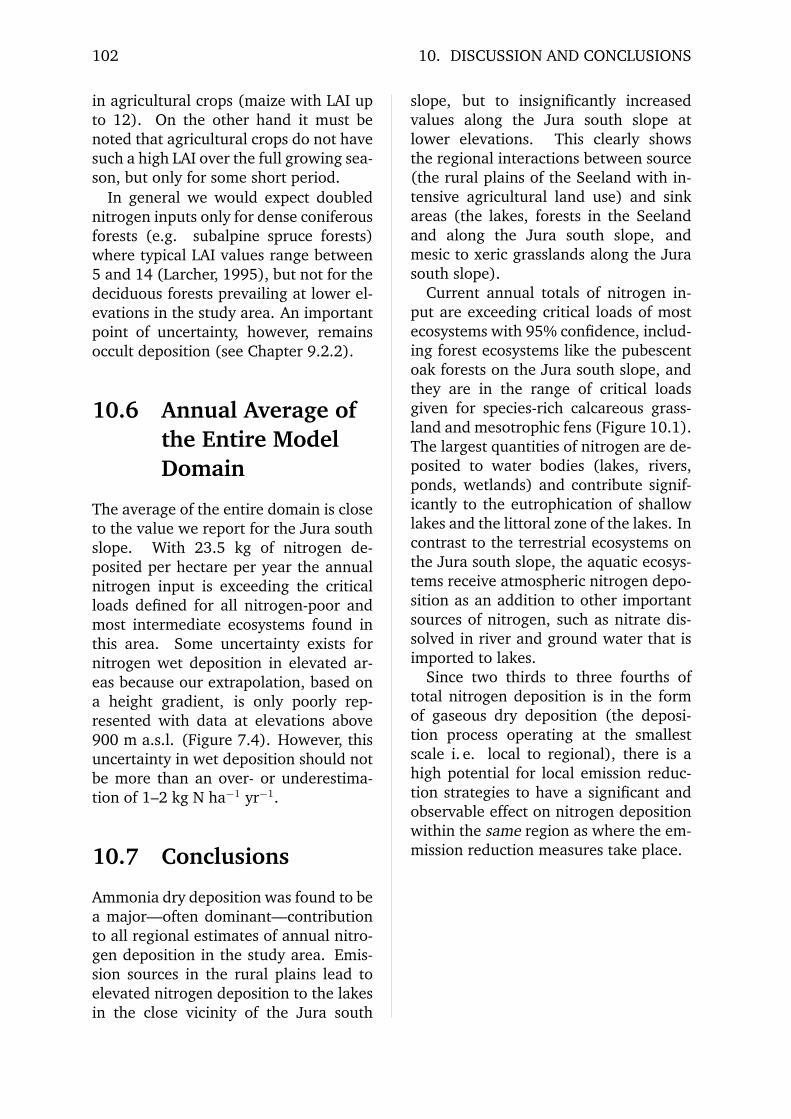
102 10. DISCUSSION AND CONCLUSIONS
in agricultural crops (maize with LAI upto 12). On the other hand it must benoted that agricultural crops do not havesuch a high LAI over the full growing sea-son, but only for some short period.
In general we would expect doublednitrogen inputs only for dense coniferousforests (e.g. subalpine spruce forests)where typical LAI values range between5 and 14 (Larcher, 1995), but not for thedeciduous forests prevailing at lower el-evations in the study area. An importantpoint of uncertainty, however, remainsoccult deposition (see Chapter 9.2.2).
10.6 Annual Average ofthe Entire ModelDomain
The average of the entire domain is closeto the value we report for the Jura southslope. With 23.5 kg of nitrogen de-posited per hectare per year the annualnitrogen input is exceeding the criticalloads defined for all nitrogen-poor andmost intermediate ecosystems found inthis area. Some uncertainty exists fornitrogen wet deposition in elevated ar-eas because our extrapolation, based ona height gradient, is only poorly rep-resented with data at elevations above900 m a.s.l. (Figure 7.4). However, thisuncertainty in wet deposition should notbe more than an over- or underestima-tion of 1–2 kg N ha−1 yr−1.
10.7 Conclusions
Ammonia dry deposition was found to bea major—often dominant—contributionto all regional estimates of annual nitro-gen deposition in the study area. Emis-sion sources in the rural plains lead toelevated nitrogen deposition to the lakesin the close vicinity of the Jura south
slope, but to insignificantly increasedvalues along the Jura south slope atlower elevations. This clearly showsthe regional interactions between source(the rural plains of the Seeland with in-tensive agricultural land use) and sinkareas (the lakes, forests in the Seelandand along the Jura south slope, andmesic to xeric grasslands along the Jurasouth slope).
Current annual totals of nitrogen in-put are exceeding critical loads of mostecosystems with 95% confidence, includ-ing forest ecosystems like the pubescentoak forests on the Jura south slope, andthey are in the range of critical loadsgiven for species-rich calcareous grass-land and mesotrophic fens (Figure 10.1).The largest quantities of nitrogen are de-posited to water bodies (lakes, rivers,ponds, wetlands) and contribute signif-icantly to the eutrophication of shallowlakes and the littoral zone of the lakes. Incontrast to the terrestrial ecosystems onthe Jura south slope, the aquatic ecosys-tems receive atmospheric nitrogen depo-sition as an addition to other importantsources of nitrogen, such as nitrate dis-solved in river and ground water that isimported to lakes.
Since two thirds to three fourths oftotal nitrogen deposition is in the formof gaseous dry deposition (the deposi-tion process operating at the smallestscale i. e. local to regional), there is ahigh potential for local emission reduc-tion strategies to have a significant andobservable effect on nitrogen depositionwithin the same region as where the em-mission reduction measures take place.

Bibliography
Arritt R. W., Pielke R. A. and Segal M.(1988) Variations of Sulfure Diox-ide Deposition Velocity ResultingFrom Terrain-forced Mesoscale Cir-culations. Atm. Environment 22,715–723.
Bloxham R. M., Hornbeck J. W. and Mar-tin C. W. (1984) The Influence ofStorm Characteristics on Sulfate inPrecipitation. Water, Air and SoilPollution 23, 359–374.
Bundesamt fur Statistik (ed.) (1992a)Eidgenossische Volkszahlung 1990:Bevolkerungsentwicklung 1850–1990, vol. 1. Bundesamt fur Statis-tik, Bern. 212 p.
Bundesamt fur Statistik (ed.) (1992b)Die Bodennutzung der Schweiz:Arealstatistik 1979/85, vol. 2. Bun-desamt fur Statistik, Bern. 227 p.
Bundesamt fur Statistik (ed.) (1994)Statistisches Jahrbuch der Schweiz.Verlag Neue Zurcher Zeitung, Zu-rich. 448 p.
Chang J. S., Brost R. A., Isaksen I. S. A.,Madronich S., Middleton P., Stock-well W. R. and Walcek C. J. (1987)Three-dimensional Eulerian AcidDeposition Model: Physical Con-cepts and Formulation. J. Geophys.Res. 92, 681–700.
Crist E. P. and Cicone R. (1984) APhysically-based Transformation ofThematic Mapper Data — The TMTasseled Cap. IEEE Transact. onGeoscience and Remote Sensing GE-22.
Ellenberg H., jun. (1990) OkologischeVeranderungen in Biozonosendurch Stickstoffeintrag. In: Am-
moniak in der Umwelt – Kreislaufe,Wirkungen, Minderung. Darmstadt,Kuratorium fur Technik undBauwesen in der Landwirtschaft,44.1–44.24.
Ellenberg H. and Klotzli F. (1972)Waldgesellschaften und Waldstan-dorte der Schweiz. Mitteilun-gen der Eidgenossischen Anstalt furdas forstliche Versuchswesen 48(4),589–930.
Ellenberg H., Weber H. E., Dull R.,Wirth V., Werner W. and PaulissenD. (1991) Zeigerwerte von Pflanzenin Mitteleuropa, vol. 18 of ScriptaGeobotanica. Erich Goltze, Gottin-gen. 248 p.
Eugster W. (1994) Mikrometeorologis-che Bestimmung des NO2-Flussesan der Grenzflache Boden/Luft. Ge-ographica Bernensia G37, 164 p.ISBN 3-906290-90-5.
Eugster W. and Hesterberg R. (1996)Transfer Resistances of NO2 De-termined From Eddy CorrelationFlux Measurements Over a LitterMeadow at a Rural Site on theSwiss Plateau. Atmospheric Envi-ronment 30(8), 1247–1254.
Eugster W., Perego S., Wanner H., Leuen-berger A., Liechti M., Reinhardt M.,Geissbuhler P., Gempeler M. andSchenk J. (1998) Spatial Variationin Annual Nitrogen Deposition in aRural Region in Switzerland. Envi-ronmental Pollution 102(S1), 327–335.
Filliger P. (1998) NABEL Luftbelastung1997, vol.303 of SchriftenreiheUmwelt. Swiss Agency for the En-
103

104 10. DISCUSSION AND CONCLUSIONS
vironment, Forests and Landscape(SAEFL), Bern. 193 p.
Furger M. (1990) Die Radiosondierungenvon Payerne: Dynamisch-klimato-logische Untersuchungen zur Ver-tikalstruktur des Windfeldes. Lenti-cularis, Opfikon (Switzerland).191 p.
Galli Purghart B. C. (1989) Schwer-metalle auf grossenfraktioniertemAerosol und in der Deposition: Un-tersuchungen an einem Hohenpro-fil im Kanton Bern. ADAG, Zurich.126 p.
Geissbuhler P. (1996) Parameter derTrockendeposition: Bestimmungdes Leaf Area Index (LAI) und desGrenzschichtwiderstands (Rb) vonFlaumeichenwaldern am Jurasud-fuss. Master’s thesis, Universityof Bern, Institute of Geography.125 p.
Gempeler M. (1997) Bestimmung derNassdeposition von Stickstoffver-bindungen im Gebiet des berni-schen Seelandes. Master’s thesis,University of Bern, Institute of Ge-ography.
Georgii H. W. and Pankrath J. (eds.)(1982) Deposition of AtmosphericPollutants. D. Reidel Publ. Comp.,Dordrecht, Holland.
Grace J. and Wilson J. (1976) TheBoundary Layer over a PopulusLeaf. J. Experimental Botany 27,231–241.
Heimgartner R. (1987) unpublished lab-oratory report. EAWAG Dubendorf,Switzerland.
Hess P. and Brezowsky H. (1969) Kata-log der Grosswetterlagen Europas.Berichte des Deutschen Wetterdienst113.
Hesterberg R., Blatter A., Fahrni M.,Rosset M., Neftel A., Eugster W.and Wanner H. (1996) Deposi-tion of Nitrogen-Containing Com-pounds to an Extensively Managed
Grassland in Central Switzerland.Environmental Pollution 91(1), 21–34.
Katz P. E. (1996) Ammoniakemissio-nen nach der Gulleanwendung aufGrunland. PhD thesis, ETH ZurichNr. 11382, Zurich. 71 p.
Keller M., Heldstab J. and KunzleT. (1997) NO2-Immissionen in derSchweiz 1990–2010, vol. 289 ofSchriftenreihe Umwelt. Federal Of-fice of Environment, Forests andLandscape, Bern. 63 p.
Krieg F. (1997) Stickstoffhaltige Gas-und Aerosolkomponenten in Pay-erne 1995, vol. 76 of Umwelt-Materialien. Federal Office of En-vironment, Forests and Landscape,Bern. 84 p.
Kunzle T. and Neu U. (1994) Exper-imentelle Studien zur raumlichenStruktur und Dynamik des Som-mersmogs uber dem SchweizerMittelland. Geographica BernensiaG7, 211 p.
Larcher W. (1995) Physiological PlantEcology. Springer, Berlin, 3rd edi-tion. 506 p.
Leuenberger A. (1996) Berechnung dergasformigen Deposition von oxi-dierten Stickstoffverbindungen imGebiet des bernischen Seelandes.Master’s thesis, University of Bern,Institute of Geography. 167 p.
Liechti M. (1996) Landnutzungskartie-rung im Gebiet des Seelandesund des angrenzenden Juras —Rechnergestutzte Erfassung derkleinraumigen Landnutzung mitmultitemporalen Landsat-5 The-matic Mapper Daten unter Ein-bezug von Arealstatistik und Pixel-karte. Master’s thesis, Universityof Bern, Institute of Geography.111 p.
Lillesand T. and Kiefer R. (1987) RemoteSensing and Image Interpretation.John Wiley & Sons, Inc., New York.
10.7 CONCLUSIONS 105
Meixner F. X. and Eugster W. (1998)In: Tenhunen and Kabat, Integrat-ing Hydrology, Ecosystem Dynam-ics, and Biogeochemistry in Com-plex Landscapes. Dahlem WorkshopReport. John Wiley & Sons Ltd.,Chichester. Effects of LandscapePattern and Topography on Emis-sions and Transport.
Menzi H., Katz P. E., Fahrni M., NeftelA. and Frick R. (1998) A Sim-ple Empirical Model Based on Re-gression Analysis to Estimate Am-monia Emissions After Manure Ap-plication. Atmospheric Environment32(3), 301–307.
Muller K. P., Aheimer G. and GravenhorstG. (1982) The Influence of Im-mediate Freezing on the ChemicalComposition of Rain-samples. In:Georgii and Pankrath, Depositionof Atmospheric Pollutants. D. ReidelPubl. Comp., Dordrecht, Holland.125–132.
Munger J. W., Fan S.-M., Bakwin P. S.,Goulden M. L., Goldstein A. H.,Colman A. S. and Wofsy S. C.(1998) Regional Budgets of Ni-trogen Oxides From ContinentalSources: Variations of Rates for Ox-idation and Deposition With Sea-son and Distance From Source Re-gions. J. Geophys. Res. 103(D7),8355–8368.
Neftel A., Wanner H., Blatter A., EugsterW., Fahrni M., Hesterberg R. andRosset M. (1994) Stickstoffeintragaus der Luft in ein Naturschutzge-biet, vol. 28 of Umwelt-MaterialienLuft. Federal Office of Envi-ronment, Forests and Landscape(FOEFL), Bern. 135 p.
Neininger B. and Dommen J. (1996)POLLUMET — Luftverschmutzungund Meteorologie in der Schweiz,vol. 63 of Umwelt-Materialien. Fed-eral Office of Environment, Forestsand Landscape, Bern. 282 p.
Perego S. (1996) Ein numerischesModell zur Simulation des Som-mersmogs. Geographica BernensiaG47, 202 p.
Perego S. (1999) MetPhoMod: A nu-merical Mesoscale Model for Sim-ulation of Regional Photosmog inComplex Terrain: Model Descrip-tion and Application During Pol-lumet 1993 (Switzerland). Meteo-rology and Atmospheric Physics ac-cepted.
Perret R. (1987) Une classificationdes situations meteorologiques al’usage de la prevision. Ar-beitsbericht der Schweiz. Meteorol.Anstalt 46, 127 p.
Posch M., de Smet P. A. M., Hettelingh J.-P. and Downing R. J. (eds.) (1995)Calculation and Mapping of Criti-cal Thresholds in Europe: Status Re-port 1995. Coordination Center forEffects, National Institute of Pub-lic Health and the Environment,Bilthoven, the Netherlands. 197 p.
Reinhardt M. (1995) Abschatzungder Emission und Deposition vonAmmoniak wahrend verschiede-ner Jahreszeiten im Gebiet desSeelandes und des angrenzendenJuras. Master’s thesis, University ofBern, Institute of Geography. 80 p.
Reiss M., Hauschild H., Rudolf B. andSchneider U. (1992) Die Behand-lung des systematischen Fehlers beiNiederschlagsmessungen. Meteo-rologische Zeitschrift 1, 51–58.
Richards J. (1993) Remote Sensing —Digital Image Analyses. An Introduc-tion. Springer Verlag, Berlin.
Rickli R. (1988) Untersuchungen zumAusbreitungsklima der Region Biel.Geographica Bernensia G32, 120 p.
Rihm B. (1996) Critical Loads of Nitrogenand their Exceedances: EutrophyingAtmospheric Deposition, vol. 275 ofEnvironmental Series. Federal Of-fice of Environment, Forests and
106 10. DISCUSSION AND CONCLUSIONS
Landscape, Bern. 82 p.SBN (ed.) (1987) Tagfalter und ihre
Lebensraume — Arten, Gefahrdung,Schutz. Schweizerischer Bund furNaturschutz (SBN), Basel. 516 p.
Schubert R. (ed.) (1991) Lehrbuch derOkologie. Gustav Fischer, Jena(Germany), 3rd edition. 657 p.
Schuepp M. (1968) Regionale Klima-beschreibungen, 1. Teil. Beiheftz. d. Ann. Schweiz. Meteorol. Zen-tralanstalt 2, 245 p.
Schumann T. (1989) Precipitation Scav-enging of Aerosol Particles: A WinterTime Field Study. PhD thesis, ETHZurich Nr. 11382, Zurich, Switzer-land. 295 p.
Slinn W. G. N., Hasse L., Hicks B. B.,Hogan A. W., Lai D., Liss P. S.,Munnich K. O., Sehmel G. A. andVittori O. (1978). Atm. Environ-ment 12, 2055.
Stadelmann F. X. (1988) Estimation ofAmmonia Losses in Swiss Agricul-ture FAO-COST joint workshop on“safe and efficient slurry utiliza-tion”. FAC Liebefeld, Bern.
Steiger P. (1994) Walder der Schweiz.Ott, Thun. 359 p.
Stevens W. K. (1996) Too Much of aGood Thing Makes Nitrogen Three-fold Menace — Atmosphere, OzoneLayer and Habitat can all SufferDamage. The New York Times (10December 1996), B5–B8.
Stockwell W. R. (1986) A HomogeneousGas Phase Mechanism for use ina Regional Acid Deposition Model.Atm. Environment 20, 1615–1632.
Stull R. B. (1988) An Introductionto Boundary Layer Meteorology.Kluwer, Dordrecht. 666 p.
Tenhunen J. D. and Kabat P.(eds.) (1998) Integrating Hydro-logy, Ecosystem Dynamics, and Bio-geochemistry in Complex LandscapesDahlem Workshop Report. JohnWiley & Sons Ltd., Chichester. In
press.Vogel S. (1970) Convective Cooling
at low Airspeed and the Shapesof Broad Leaves. J. ExperimentalBotany 21, 91–101.
Walcek C. J., Brost R. A. and Chang J. S.(1986) SO2, Sulfate and HNO3 De-position Velocities Computed UsingRegional Landuse and Meteorolog-ical Data. Atm. Environment 20,949–964.
Wanner H. and Furger M. (1990) TheBise — Climatology of a RegionalWind North of the Alps. Meteorol.Atmos. Phys. 43, 105–115.
Wanner H. (1979) Zur Bildung, Ver-teilung und Vorhersage winter-licher Nebel im Querschnitt Jura–Alpen. Geographica Bernensia G7,240 p.
Wanner H. and Kunz S. (1977) DieLokalwettertypen der Region Bern.Beitr. zum Klima der Region Bern 9,96 p.
Wesely M. L. (1989) Parametrization ofSurface Resistances to Gaseous DryDeposition in Regional-Scale Nu-merical Models. Atmospheric Envi-ronment 23, 1293–1304.
Wilks D. S. (1995) Statistical Methods inthe Atmospheric Sciences. AcademicPress, San Diego. 467 p.
Winkler P., Jobst S. and HarderC. (1989) Meteorologische Prufungund Beurteilung von Sammelgeratenfur die nasse Deposition, vol.1/89 ofBPT-Bericht. GSF, Munchen. 315 p.
Zbinden N., Imhof T. and Pfister H. P.(1987) Ornithologische Merkblatterfur die Raumplanung. Schweize-rische Vogelwarte, Sempach,Switzerland.

Index
afforestation, 29algae, growth of, 29Altweibersommer, 36ammonia emissions, 55, 56, 93ammonia loss, 53ANETZ, 49, 58arable land, 32atmospheric chemistry, 39atmospheric inputs, 29atmospheric processes, 22
BAT, 77Belpmoos, 75Bise, 36, 51boundary conditions, 40Burgdorf, 65butterflies, 27, 30
potential impact on, 28
catalytic converters, 24cattle density, 25Chasseral, 51Chasseral (mount), 25COMRAD, 58concentration, trend over last 10 years, 93critical levels, 21critical loads, 21–23, 96, 99
deposition, 40, 96–102aerosol, see deposition, drydry, 21, 22, 38, 39, 41, 46, 48, 49, 52,
59–74, 85–92module, 40occult, 95, 102total, 21uncertainty over water surface, 94wet, 21, 22, 75–84
deposition velocity, 93diffusion, 40, 41
molecular, 41
economic loss, 24ecosystem
aquatic, 22, 102natural, 17
nitrogen pools, 17nitrogen-poor, 102nutrient-poor, 17, 18, 21–24, 29rare, 24semi-natural, 17, 22species-rich, 26terrestrial, 21, 22
EMEP, 21, 23, 40, 57, 96emission factor, 53, 55, 56, 93emission inventory, 40, 54, 93enery fluxes, 46
fluttering (leaves), 41fog, 36fog interception, see deposition, occultfogginess, 36forest
decline, 18types, 26
Gewasserkorrektion, see leveeinggrassland, 29
species-rich, 27Green Revolution, 21
heterogeneous chemistry, 95human activities, 21, 23human activity, 17
imports, 97Indian Summer, see Altweibersommer
Jolimont, 77Jura mountain range, 25, 29Juragewasserkorrektion, see leveeingJaissberg, 65
Kerzersmoos, 77
lake shore, 22, 29land use pattern, 31Landsat, 31, 32landscape evolution, 29LBL, 54Le Landeron, 77
107
108 INDEX
leveeing, 29Liebefeld, 75Lignieres, 78local names, 60long-range transports, 97low-NOX, 24Langenberg, 75
manure, 23, 27, 52, 55storage of, 54
Merenschwand, 21, 23model domain, 39, 51Moleson, 51
NABEL, 75, 79, 84, 89Napf, 51nitrogen
dissolved, 22inert gaseous, 21molecular, 17oxidized, 17, 24plant available, 17reduced, 17
nitrogen cycle, 21, 22, 24, 29nitrogen deposition, 24
pastures, 69Payerne, 51, 75, 79, 84photochemical cycle, 38Plaffeien, 51plant
endangered species, 17, 18nitrogen-fixing, 21species diversity, 25, 26
population density, 24precipitation, 32pressure gradient, 40, 57pubescent oak forests, 99
radiosonde, 45, 48, 57, 58RADM, 39rain droplet sensor, 75, 76ratio of reduced to total nitrogen, 96reeds, 29reference days, 49regions, defined, 62resistance
aerodynamic, 41canopy, 44laminar boundary layer, 41model, 42
Reuss valley, 21
RVI, 32
seasons, 44, 45Siselen, 77slurry, 23smog (summer), 38snowfall, 36Studen, 65susceptibility, 19, 22
tasseled cap transformation, 32Taubenloch gorge, 65temperature, 36thermal inversion, 49, 51, 65, 74time period (1990–1994), 96time step, 39topography, 39, 40, 60traffic
aircraft, 17motorized, 17
transilient turbulence, 39transports
long-range, 57turbulent dispersion, 96turbulent transport, 93, 96
class, 52conditions, 48
validation, 41, 45vegetation
current, 28potential, 25, 28
Waldschaden, see forest declinewaste incinerators, 17waste water treatment, 22water stress, 46weather classification, 48wet-only sampler, 75, 76
collection efficiency, 76wetland birds, 29wetland habitats, 29, 30woodlark, 28, 29Worben, 65
Zihl river, 65

A. Color Plates
The color plates presented here are ref-erenced and discussed in Chapters 3, 5,6, and 10. The text in this Appendixis therefore only supposed to help thereader quickly understand what the in-dividual color plates display. For adeeper understanding of the contents ofthe plates the reader is referred to thecorresponding chapters.
Land Use Classification1994
On page 111 (Plate A.1) the land-useclassification by Liechti (1996) is shownat full resolution. For modeling pur-poses the full resolution derived fromsatellite imaginery was aggregated to1×1 km2 cells. Liechti (1996) alsoproduced an intermediate resolution of1 ha (100×100 m2; not shown). PlateA.1 indicates at which scale the land-usecould be resolved in future modelingstudies; however, to benefit from thisincreased resolution, Metphomod willhave to be adapted to this finer scale,and model parameters for the land-usetypes thus resolved must then be deter-mined.
Ammonia EmissionInventory
The color plates on pages 112–113 showthe annual and seasonal ammonia emis-sions calculated by Reinhardt (1995). InPlate A.2 the two methods used by Rein-hardt are compared for the annual to-
tals. Plate A.3 shows the semi-monthlyaverage emissions during the five modelseasons.
Total Annual NitrogenDeposition
The color plate on page 114 shows thespatial pattern of total annual nitrogendeposition (the sum of gaseous dry de-position, wet deposition, and dry partic-ulate aerosol deposition) for the studyarea (Plate A.4).
For this and al following plates themodel domain is oriented from thenorthwest at top to southeast at the bot-tom (40◦ rotation angle between mapnorth and geographic north). The exactposition of the model domain is shownin Figure 5.1 on page 51.
Dry Deposition ModelResults
Annual Totals of Nitrogen DryDeposition
The color plates on pages 115–117 showthe annual total of nitrogen dry deposi-tion (modelled with Metphomod). Forall color plates on pages 115–122 thecolor coding is from green (low values)to red (high values). However it is tobe noted that the color classes are notequally spaced in all plates so as to im-prove readability. All deposition valuesare given in kg N ha−1 yr−1.
109
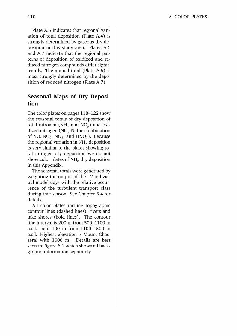
110 A. COLOR PLATES
Plate A.5 indicates that regional vari-ation of total deposition (Plate A.4) isstrongly determined by gaseous dry de-position in this study area. Plates A.6and A.7 indicate that the regional pat-terns of deposition of oxidized and re-duced nitrogen compounds differ signif-icantly. The annual total (Plate A.5) ismost strongly determined by the depo-sition of reduced nitrogen (Plate A.7).
Seasonal Maps of Dry Deposi-tion
The color plates on pages 118–122 showthe seasonal totals of dry deposition oftotal nitrogen (NHx and NOy) and oxi-dized nitrogen (NOy-N, the combinationof NO, NO2, NO3, and HNO3). Becausethe regional variation in NHx depositionis very similar to the plates showing to-tal nitrogen dry deposition we do notshow color plates of NHx dry depositionin this Appendix.
The seasonal totals were generated byweighting the output of the 17 individ-ual model days with the relative occur-rence of the turbulent transport classduring that season. See Chapter 5.4 fordetails.
All color plates include topographiccontour lines (dashed lines), rivers andlake shores (bold lines). The contourline interval is 200 m from 500–1100 ma.s.l. and 100 m from 1100–1500 ma.s.l. Highest elevation is Mount Chas-seral with 1606 m. Details are bestseen in Figure 6.1 which shows all back-ground information separately.

A. COLOR PLATES 111
open
wat
er
whe
at
barle
y
rye
rape
pota
toes
corn
/mai
ze
suga
r be
ets
soy
bean
s an
d pe
as
oat
toba
cco
unkn
own
gene
ral l
and
use
vine
yar
ds
orch
ards
hort
icul
ture
mea
dow
s an
d pa
stur
es
ripar
ian
vege
tatio
n
resi
dent
ial a
reas
(r.
a.)
high
den
sity
r.a
.
med
ium
den
sity
r.a
.
low
den
sity
r.a
.
mis
cella
neou
s r.
a.
road
s
railr
oads
air
field
s
coni
fero
us fo
rest
mix
ed fo
rest
deci
duou
s fo
rest
coni
fero
us m
ixed
fore
st (
Jura
)
deci
duou
s m
ixed
fore
st (
Jura
)
deci
duou
s fo
rest
(Ju
ra)
Plate A.1: Landsat TM multitemporal and multispectral land use classification for 1994 (corre-sponding with Table 3.2). North is at left.
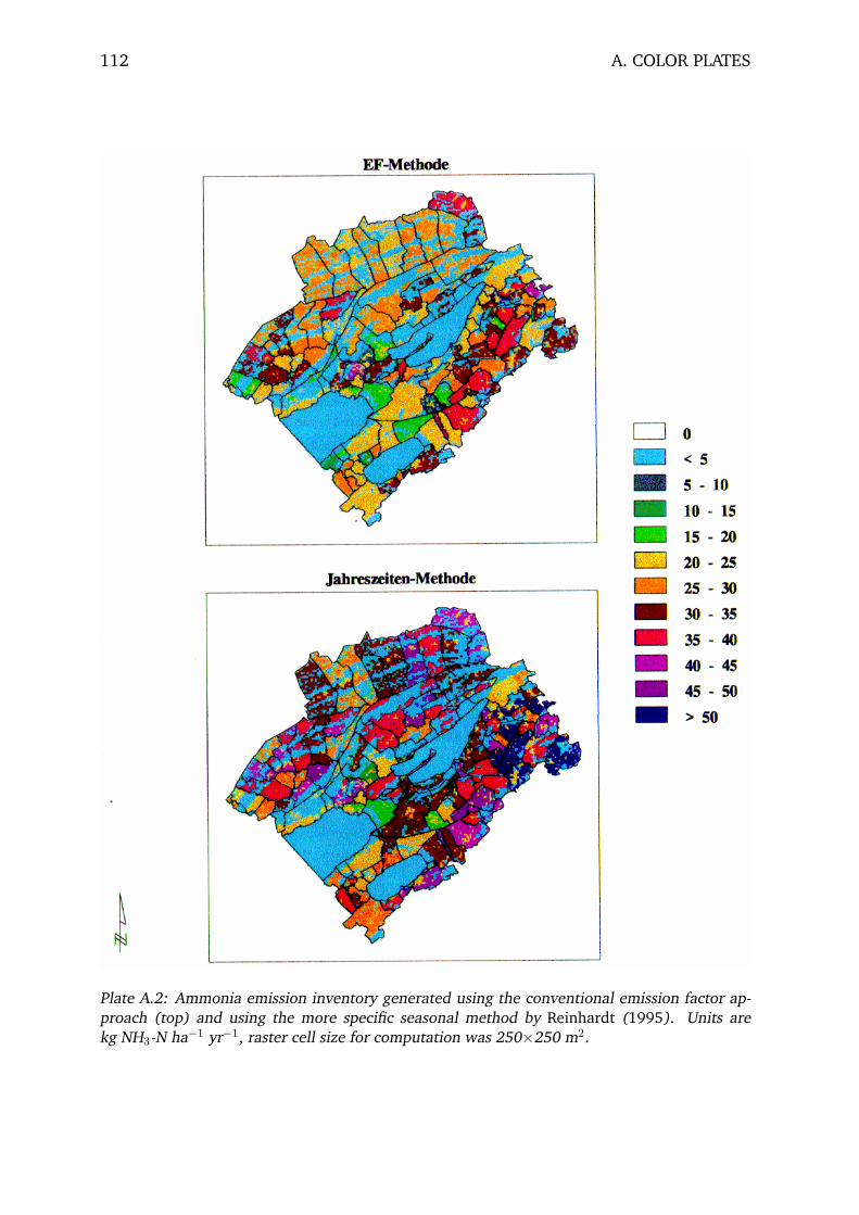
112 A. COLOR PLATES
Plate A.2: Ammonia emission inventory generated using the conventional emission factor ap-proach (top) and using the more specific seasonal method by Reinhardt (1995). Units arekg NH3-N ha−1 yr−1, raster cell size for computation was 250×250 m2.
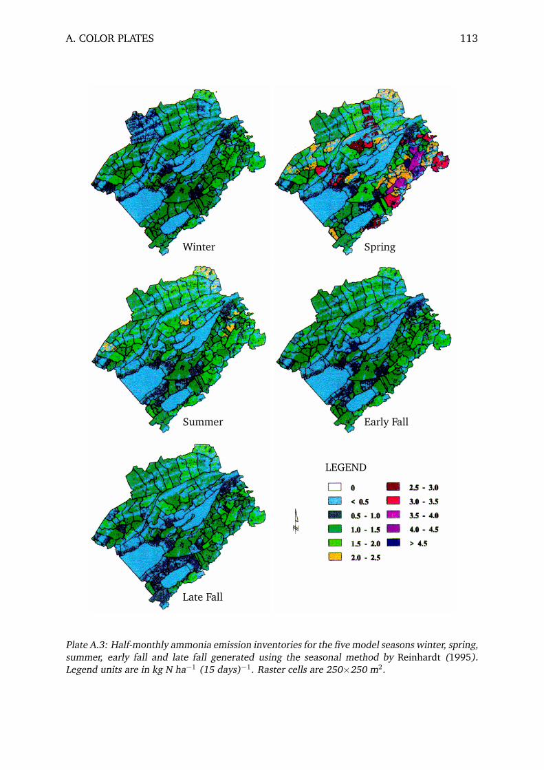
A. COLOR PLATES 113
Winter Spring
Summer Early Fall
Late Fall
LEGEND
Plate A.3: Half-monthly ammonia emission inventories for the five model seasons winter, spring,summer, early fall and late fall generated using the seasonal method by Reinhardt (1995).Legend units are in kg N ha−1 (15 days)−1. Raster cells are 250×250 m2.

114 A. COLOR PLATES
Total Annual Nitrogen Deposition
Plate A.4: Total annual nitrogen deposition of gaseous dry deposition, wet deposition andaerosol deposition (sedimentation and impaction) in kg N ha−1 yr−1.

A. COLOR PLATES 115
Annual Totals of Nitrogen Dry Deposition
Plate A.5: Total annual nitrogen dry deposition.
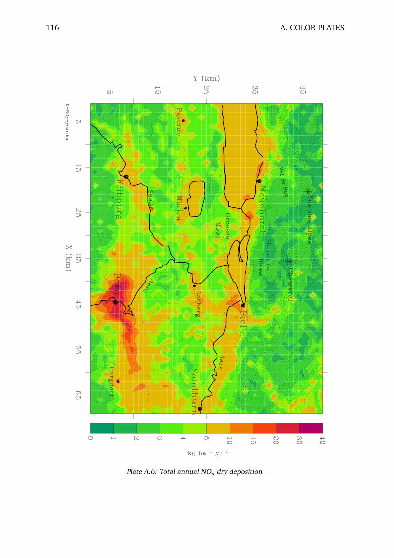
116 A. COLOR PLATES
Plate A.6: Total annual NOy dry deposition.
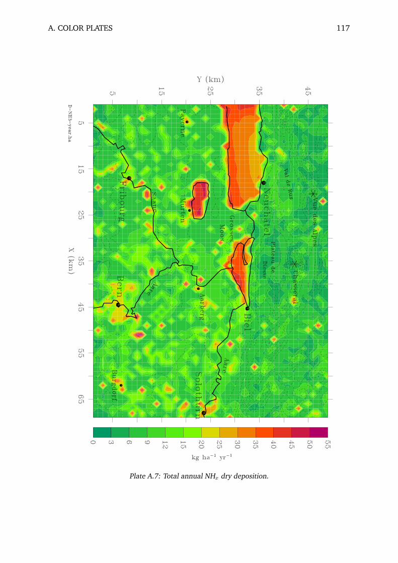
A. COLOR PLATES 117
Plate A.7: Total annual NHx dry deposition.
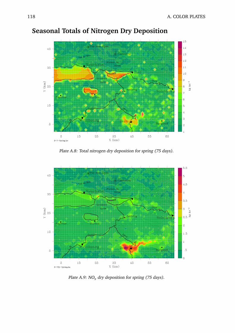
118 A. COLOR PLATES
Seasonal Totals of Nitrogen Dry Deposition
Plate A.8: Total nitrogen dry deposition for spring (75 days).
Plate A.9: NOy dry deposition for spring (75 days).

A. COLOR PLATES 119
Plate A.10: Total nitrogen dry deposition for summer (61 days).
Plate A.11: NOy dry deposition for summer (61 days).
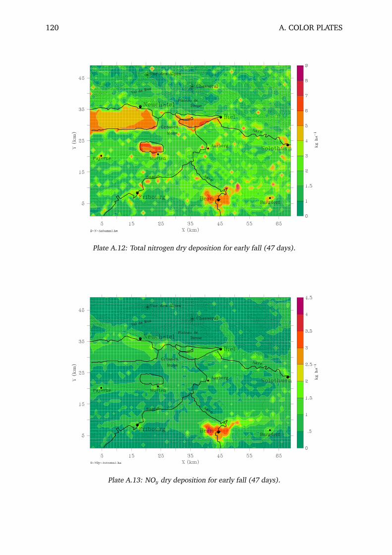
120 A. COLOR PLATES
Plate A.12: Total nitrogen dry deposition for early fall (47 days).
Plate A.13: NOy dry deposition for early fall (47 days).

A. COLOR PLATES 121
Plate A.14: Total nitrogen dry deposition for late fall (61 days).
Plate A.15: NOy dry deposition for late fall (61 days).
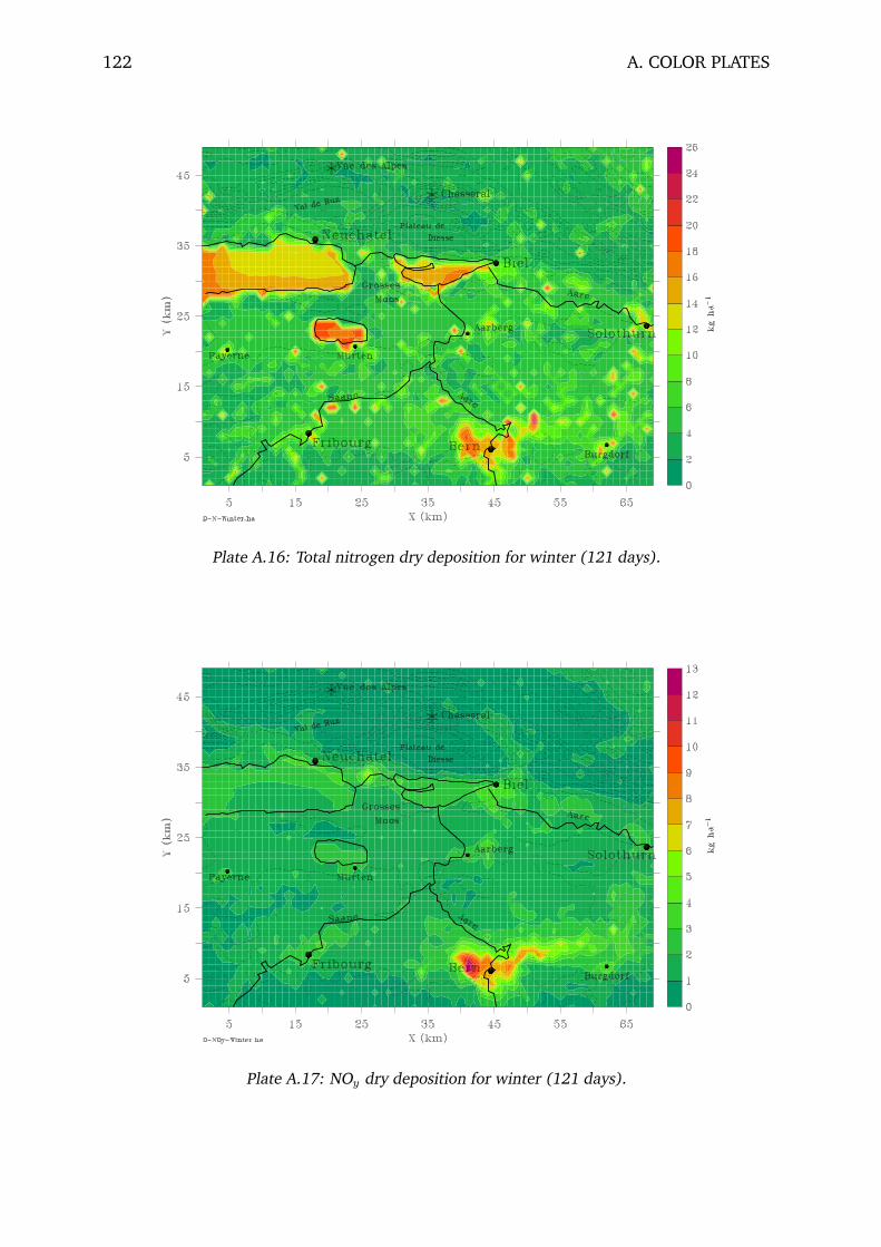
122 A. COLOR PLATES
Plate A.16: Total nitrogen dry deposition for winter (121 days).
Plate A.17: NOy dry deposition for winter (121 days).