Atmospheric emissions from vegetation fires in Portugal (1990–2008

Atmos. Chem. Phys., 11, 2625–2640, 2011www.atmos-chem-phys.net/11/2625/2011/doi:10.5194/acp-11-2625-2011© Author(s) 2011. CC Attribution 3.0 License.

AtmosphericChemistry

and Physics

Atmospheric emissions from vegetation fires inPortugal (1990–2008): estimates, uncertainty analysis,and sensitivity analysis

I. M. D. Rosa1,*, J. M. C. Pereira1, and S. Tarantola2

1Technical University of Lisbon, School of Agriculture, Center for Forest Studies, Tapada da Ajuda,1349-017 Lisboa, Portugal2Joint Research Centre of the European Commission, Ispra, Italy* now at: Faculty of Natural Sciences, Division of Biology, Imperial College of London, Silwood Park Campus, UK

Received: 25 June 2010 – Published in Atmos. Chem. Phys. Discuss.: 22 September 2010Revised: 31 January 2011 – Accepted: 10 March 2011 – Published: 21 March 2011

Abstract. Atmospheric emissions from wildfires in Portu-gal were estimated yearly over the period 1990–2008 usingLandsat-based burnt area maps and land cover maps, nationalforest inventory data, biometric models, and literature reviewdata. Emissions were calculated as the product of area burnt,biomass loading per unit area, combustion factor, and emis-sion factor, using land cover specific values for all variables.Uncertainty associated with each input variable was quanti-fied with a probability density function or a standard devia-tion value. Uncertainty and sensitivity analysis of estimateswere performed with Monte Carlo and variance decomposi-tion techniques. Area burnt varied almost 50-fold during thestudy period, from about 9000 ha in 2008 to 440 000 ha in2003. Emissions reach maximum and minimum in the sameyears, with carbon dioxide equivalent (CO2eq.) values of 159and 5655 Gg for 2008 and 2003, respectively. Emission fac-tors, and the combustion factor for shrubs were identifiedas the variables with higher impact on model output vari-ance. There is a very strong correlation between area burntand emissions, allowing for good emissions estimates oncearea burnt is quantified. Pyrogenic emissions were comparedagainst those from various economy sectors and found to rep-resent 1% to 9% of the total.

Correspondence to:I. M. D. Rosa([email protected])

1 Introduction

Environmental impacts of wildfires affect abiotic and bioticecosystem components, including flora, fauna, soil, water,air, and cultural resources (Brown and Smith, 2000). Fromthe standpoint of atmospheric impacts, land use and naturalresource managers need timely, accurate information to as-sess, monitor, and predict emission magnitudes and air qual-ity impacts, namely from prescribed burning programs, acutehealth effects of smoke exposure, visibility reduction, and toassess tradeoffs between air quality impacts from wildlandfire and prescribed fire (Sandberg et al., 2002).

Several studies have analysed various aspects of the at-mospheric impacts of wildfires in Europe, ranging from themore general, such as air quality issues (Miranda et al.,2009a) and emissions assessment (Barbosa et al., 2009), tomore specific or local, including particulate matter emis-sions, transport, and radiative effects (Hodzic et al., 2007),mercury emissions (Cinnirella and Pirrone, 2006), emissionsand global warming relationships (Miranda et al., 1994), theimpact of Eastern European agricultural fires on Arctic airpollution (Stohl et al., 2007), and satellite tracking of emis-sion and transport of pollution from an extreme fire episode(Turquety et al., 2009). Barbosa et al. (2009) presented ananalysis of wildfire numbers and area burnt in Europe us-ing data from the European Forest Fire Information Sys-tem (EFFIS), which show that an annual average (2000–2005) of about 95 000 fires occurred and 600 000 ha wereburnt in 23 European countries. About two-thirds of the fireswere recorded in five southern European countries (France,Greece, Italy, Portugal, and Spain) where an annual averageof about 500 000 burnt every year. Their pyrogenic carbon

Published by Copernicus Publications on behalf of the European Geosciences Union.

http://creativecommons.org/licenses/by/3.0/

2626 I. M. D. Rosa et al.: Emissions from vegetation fires

dioxide (CO2) annual emissions estimates for the 23 Euro-pean countries were 8.4 to 20.4 Tg year−1.

A few studies have dealt with pyrogenic emissions in Por-tugal. Miranda et al. (1994) estimated CO2 emissions dueto wildfires and found that in years when the burnt area ex-ceeds 100 000 ha this contribution could reach 7% of the totalPortuguese CO2 emissions. Miranda et al. (2009a) modelledsmoke plume impact on urban air quality in Lisbon duringthe extreme 2003 fire season and obtained results in reason-able agreement with those observed at ground-based moni-toring networks. Miranda et al. (2009b) modeled air qualityover the entire area of Portugal during August 2003, usingan operational 3-D chemistry transport model. Results werecompared with monitoring data from regional air quality net-works, and were found to improve substantially where wild-fire emissions were included, namely for particulate matterand ozone (O3). Pio et al. (2008) collected aerosol samplesin central coastal Portugal, also during the summer 2003 ex-treme fire season, when over 400 000 ha of forests, shrub-lands and agricultural areas were burnt. During this period,aerosol samples were analysed for total mass and for a setof inorganic and organic compounds, including tracers ofbiomass burning. From organic C-to-levoglucosan or organicC-to-K ratios it was estimated that 40 to 55% of primary or-ganic C could be attributed to wood smoke. Studies by Silvaet al. (2006) and Pio et al. (2006), which estimated pyrogenicemissions in Portugal during the 1990s, are direct precursorsto the present analysis. Silva et al. (2006) estimated CO2equivalent emissions ranging from a low of 0.474 Mt in 1997to a maximum of 3869 Mt CO2eq. in 1998. CO2eq. is a univer-sal measurement to evaluate the impact of releasing differentgreenhouse gases to the atmosphere. Each greenhouse gas(GHG) has a global warming potential (GWP), which esti-mates the impact of a chemical species in global warming,when compared to the impact of CO2 (which has a GWP of1). A linear regression model between annual area burnt andCO2eq. emissions for the 1990s led to an estimate of 7.39 MtCO2eq. emitted during the record area burnt year 2003. Theyalso calculated that the amount of GHG released by wild-fires in 1991 corresponded to 22.4% of that emitted by theenergy sector, 44.2% of the manufacturing and constructionactivities, 32.9% of the transport sector, 31.1% of that re-leased by agriculture, and 81% of industrial activity emis-sions. Pio et al. (2006) estimated pyrogenic dioxin emissionsas the second largest source for this pollutant at the nationallevel (17%).

Most biomass burning emission studies rely on the modeldeveloped by Seiler and Crutzen (1980), which combines in-formation on above-ground biomass available for burning,combustion factors, burning area, and emission factors fora certain species and vegetation type, to calculate the py-rogenic emissions (Wooster et al., 2005). However, thesevariables are hard to estimate, which causes large uncertain-ties in results. Recently introduced methodologies based onsatellite measurements, are meant to improve these estimates

(Wooster et al., 2004). Recent biomass burning studies bothat regional (e.g. Pereira et al., 2009a) and global scales (e.g.Kaiser et al. 2009) rely on the relationship between fire radia-tive power (FRP), biomass consumed during a wildfire event,and smoke aerosol emission factor to provide estimates ofthe total amount of aerosol and trace gases emitted into theatmosphere (Woodster et al., 2005; Freeborn et al., 2008;Pereira et al., 2009a). These new methods are especially im-portant to overcome one of the main limitations of traditionalmethods: the difficulty in obtaining near real-time emissionsestimates. Despite their advantages, these new methodolo-gies still have uncertainties attached. The FRP satellite prod-ucts, both from the Moderate Resolution Imaging Spectrora-diometer (MODIS) and from the Geostationary OperationalEnvironmental Satellites (GOES), require complex valida-tions, yet unavailable. In addition, they also suffer from tech-nical problems such as channel saturation, undetected fires,and cloud cover, among others (Pereira et al., 2009a).

Schultz et al. (2008) considered that three main factors ofuncertainty limit the accuracy of long-term, global biomassburning emission data sets. These factors, also relevant atthe regional scale of the present study, are the accuracy ofestimates of burnt area, combustion completeness, and emis-sion factors. The effect of burnt area uncertainty on pyro-genic emission estimates was taken into account by Barbosaet al. (1999), and by Korontzi et al. (2004), using two differ-ent burnt area spatial datasets. Burnt area maps used hereinwere derived from much higher spatial resolution satelliteimagery, and checked for accuracy against field data. Useof a country-wide, long-term, high accuracy burnt area geo-graphical dataset is an important asset of the present study.From a methodological standpoint, another relevant contri-bution of this study is the use of a formal uncertainty andsensitivity assessment approach that is much more sophis-ticated than the error analysis approach used by Scholes etal. (1996), Levine (1996), and Barbosa et al. (1999).

The objectives of the present study are to estimate atmo-spheric emissions from wildfires in Portugal over the last twodecades, to assess the uncertainty inherent in those estimates,and to identify the main sources of uncertainty. We rely on acombination of burnt area maps and land cover maps derivedfrom remotely sensed data, forest inventory data, statisticalgrowth models for forests and shrublands, and results fromthe literature for combustion factors, emissions factors, andfor biomass of some land cover types.

2 Study area

Portugal is located between latitude 37◦ N and 42◦ N andbetween longitude 9.5◦ W and 6.5◦ W. Climate is temper-ate, typically hot and dry during the summer, and cooland wet in winter. Topography is rugged, especially inthe northern half of the country, and most vegetation coveris evergreen, drought resistant, and pyrophitic. These

Atmos. Chem. Phys., 11, 2625–2640, 2011 www.atmos-chem-phys.net/11/2625/2011/

I. M. D. Rosa et al.: Emissions from vegetation fires 2627

environmental features make the region susceptible to veg-etation fires, a characteristic that has been reinforced duringthe last four or five decades by demographic, socio-economic(Mather and Pereira, 2006) and climatic trends (Pereira etal., 2002). Since the 1960s many countryside areas have suf-fered substantial population losses, abandonment of agricul-tural fields, reduction of goat and sheep herds, resulting ina decrease in grazing, and lowered use of fuel wood. Thus,progressive accumulation of fine fuels has been occurring inforests and woodlands that previously were cleared of under-brush. Given the decrease in agricultural activity, large areasof marginal productivity were converted to forest or aban-doned to old-field succession.

About one-third of the area of Portugal is covered byforests and woodlands. Maritime pine (Pinus pinaster)forests are located mainly in the northern half of the country,while Eucalypt (Eucalyptus globulus) forests are widespreadin western Portugal, and in a few inland areas, in the centraland southern parts of the country. Evergreen oak woodlandspredominate in the south. Cork oak (Quercus suber) wood-lands are the tree land cover type in SW Portugal and alongthe Tagus river valley, while Holm oak (Quercus rotundifo-lia) predominates in the SE. Agricultural areas occupy abouthalf of the country and, although widespread, dominate inthe central coastal plain, along main river valleys, and inthe south. Central and northern Portugal agricultural land-scapes are a mosaic of diverse crops, vineyards, and olivegroves. Agriculture in southern Portugal is dominated by dryland farming of cereal crops. Most shrublands are located innorthern and eastern Portugal, but also occur in other regions,usually mountainous and/or sparsely populated.

3 Data and methods

Calculation of GHG (carbon dioxide (CO2), nitrous oxide(N2O), and methane (CH4)), other trace gases and aerosolspyrogenic emissions in Portugal between 1990 and 2008 re-lied on the model of Seiler and Crutzen (1980):

Ea =

∑i

∑n

AiBniαniEFa (1)

whereEa is the mass emitted of chemical speciesa (kg), Ai

is the burnt area on land cover classi (ha),Bni is the biomassof the n component on the land cover classi (Mg ha−1), α

is the combustion factor (%), andEF is the emission factor(kg Mg−1).

However, there are important uncertainties associated withestimates of these variables. Area burnt uncertainty is causedby large inter-annual variability and inaccuracies in satellite-based burnt area mapping. Uncertainties associated withbiomass, combustion factors, and emissions factors are theresult of sampling error and large variability in fire be-haviour and effects on diverse vegetation types. Values for

Table 1. Land cover classes used to determine burnt area. Theseclasses were aggregated into three main groups on the basis ofmethodological similarities for biomass estimation.

Land cover classes

Forest Maritime pineUmbrella pineEucalyptCork oakHolm oakOther ConiferOther BroadleavedMixed (Maritime pineand Eucalypt)Mixed (Eucalypt andCork oak)∗

Agriculture AgroforestryOrchardVineyardAnnual cropsOlive grovesHeterogeneous cropsSparsely vegetated

Shrublands Shrublands and grasslandsBurnt more than once

∗ only for the 2000–2008 period

the variables in Eq. (1) were obtained from a combination ofin-house data, literature review, and model-based estimates.We performed an uncertainty and sensitivity analysis to as-sess the dependence ofEa on values of the input variables.

3.1 Burnt area

Burnt area in each land cover class and each year wasestimated using the approach of Pereira and Santos (2003),which assumes that there are no land-use changes, apartfrom fire, during the period considered. Due to thisassumption and the existence of different land coverdatasets, with different spatial resolutions, the analysiswas split into two periods: for the 1990s, we used aland cover map derived from aerial photo-interpretation,with a spatial resolution of 1:25 000 and minimum map-ping unit of 1 ha (Portuguese Geographic Institute, URLhttp://www.igeo.pt/produtos/CEGIG/COS.htm). From 2000to 2008, the analysis of annual fire incidence by landcover type relied on the CORINE2000 land cover mapof Portugal, with a spatial resolution of 1:100 000 and aminimum mapping unit of 25 ha (European EnvironmentAgency, URL http://www.eea.europa.eu/data-and-maps/figures/corine-land-cover-2000-by-country-1). We deriveda common, simplified legend for the two maps, whichwas deemed adequate for estimating pyrogenic emissions

www.atmos-chem-phys.net/11/2625/2011/ Atmos. Chem. Phys., 11, 2625–2640, 2011

http://www.igeo.pt/produtos/CEGIG/COS.htm

http://www.eea.europa.eu/data-and-maps/figures/corine-land-cover-2000-by-country-1

http://www.eea.europa.eu/data-and-maps/figures/corine-land-cover-2000-by-country-1


(Table 1). The land cover maps for each analysis periodwere updated with the areas burnt annually, designated bythe corresponding fire year.

The CORINE2000 land cover map legend only consid-ers three main forest classes (“Broadleaved”, “Conifer” and“Mixed”), which are too broad for emissions assessment,since each class contains forest types that are very differentin structure, biomass, and vulnerability to fire. Therefore,we used data from the 2005–2006 National Forest Inventory(NFI) field plots to split these overly broad classes into ho-mogeneous forest types, from the standpoint of emissions as-sessment.

The modified land cover map of Portugal was overlainwith the fire perimeter atlas to quantify the area burnt an-nually in each land cover type. The fire perimeter atlas usedin the present study is derived from Landsat satellite imageryfor the period between 1990 and 2008, with a spatial reso-lution of 30 m and a minimum mapped unit of 5 ha (Pereiraand Santos, 2003). The procedure is semi-automatic, start-ing with a supervised approach using classification trees, fol-lowed by on-screen editing of classification results. The finalstep – validation – is made by comparing the results againstthe Portuguese official field statistics (National Forest Au-thority, URL: http://www.afn.min-agricultura.pt/portal/dudf/estatisticas) at the parish and county level.

3.2 Biomass estimation

Estimating biomass fuel loadings is complex due to the highspatial heterogeneity and dynamic character of vegetation.For the sake of simplicity, all land cover classes were ag-gregated into three main groups (Forests, Shrublands andAgriculture), on the basis of methodological similarities forbiomass estimation (Table 1).

3.2.1 Forests

Forest fires can affect one or more fuel strata, including litter,surface fuels, and tree crowns. We considered four compo-nents of the total forest biomass: litter, understory shrubs,tree crown leaves and fine (<2 cm Ø) branches. We as-sume that woody fuels>2cm Ø are not consumed by wild-fires, which may underestimate emissions under extreme fireseverity.

Forest litter fuel loadings were obtained from a literaturereview (Table 2). These values are from temperate ecosys-tems and are separated by different types of forest cover. Thefact that only one study quantifies litter for Umbrella pineforests in the Mediterranean (Stamou et al., 1998), preventedus from including this variable in the uncertainty and sensi-tivity analysis.

NFI field plots provide data on understory shrub speciescomposition, percent cover, and mean height. Equation (2)combines these data with species-specific bulk density (Silva

et al., 2006), to yield understory shrub fuel loading perhectare:

Bj =

6∑1

ρbsPcsiAi (2)

where Bj represents the shrubs biomass in the plotj

(kg m−2), ρbs is the bulk density of shrubs species s(kg m−3), Pcsi is the percent cover speciess on height classi (%), andAi is the class height (m).

In order to determine the crown biomass we first had toestimate the trees’ height, using hypsometric equations (Na-tional Forest Authority, 2010), since the NFI only describesthe height of the dominant trees. Afterwards, we applieda set of equations from the Portuguese NFI (Correia et al.,2008 and National Forest Authority, 2010) to estimate theleaves biomass. For some species (Cork oak, Holm oak andother broadleaved) we used the equations from the SpanishNFI (Montero et al., 2005), since the Portuguese NFI doesnot provide leaf biomass equations for these species. Finally,to determine the fine branches biomass, we applied SpanishNFI equations (Montero et al., 2005), since the PortugueseNFI equations for branches biomass do not differentiate di-ameter classes.

3.2.2 Shrublands

This broad group includes the “Shrublands and grasslands”class, as well as those areas burnt at least twice during the pe-riod under analysis (“Burnt more than once”), and considerstwo components, namely litter and shrubs.

Estimation of total shrubland biomass relied on Ol-son’s (1963) model and the field data gathered bySimoes (2006), relating shrubland biomass and age. Olson’smodel is given by:

Wshb= a(1−e−bt

)(3)

whereWshb is shrub biomass (Mg ha−1), a represents max-imum fuel load (Mg ha−1) andb is the time since last fire(years). Parametersa andb were estimated with an ordinaryleast squares model fit. Confidence intervals (95%) of the pa-rameters estimated mean value were calculated as well as theroot mean square error of the model fitted, which quantifiesthe error associated to the predictions of shrub biomass.

Using Eq. (3) requires knowledge of the shrub patch age.We can determine age at the time of burning for the patchesthat burnt at least twice during the study period. However, weignore the age of the ”Shrublands and grasslands” patches atthe time they burn during our study period. Therefore, it wasnecessary to estimate a mean patch age, for input into Olson’smodel. That was done using the methodology of Johnson andGutsell (1994):

APL = b

γ(

2c

)γ

(1c

) (4)


http://www.afn.min-agricultura.pt/portal/dudf/estatisticas

http://www.afn.min-agricultura.pt/portal/dudf/estatisticas


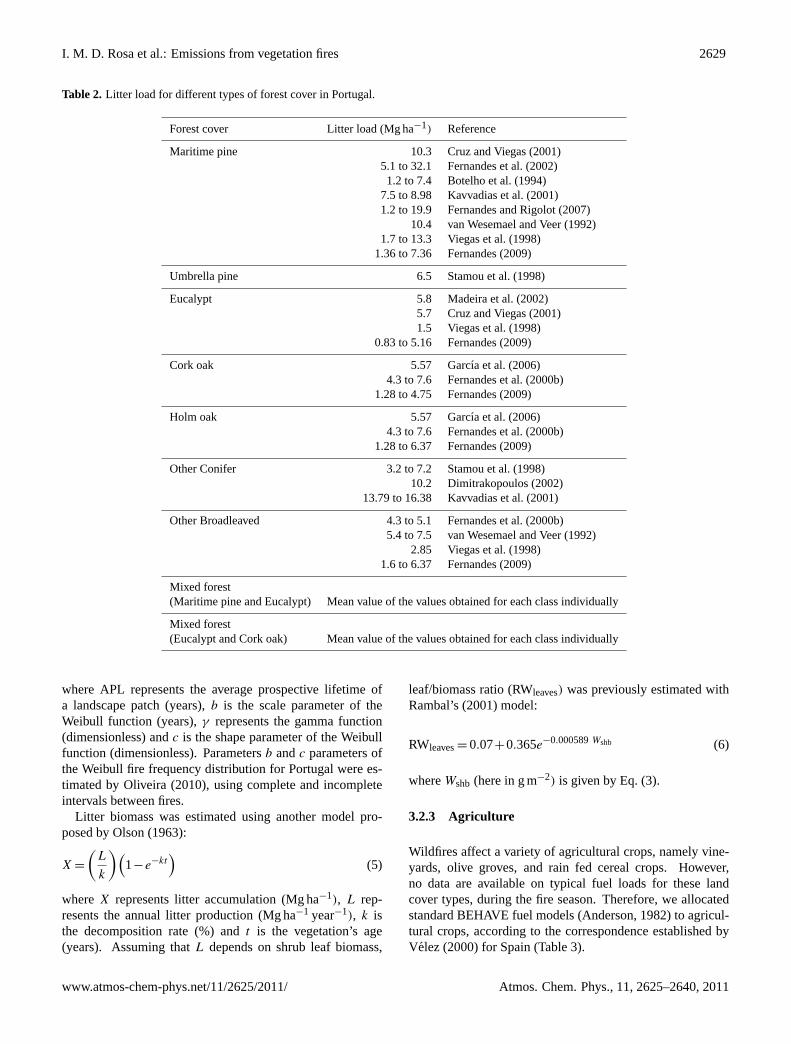
Table 2. Litter load for different types of forest cover in Portugal.

Forest cover Litter load (Mg ha−1) Reference

Maritime pine 10.3 Cruz and Viegas (2001)5.1 to 32.1 Fernandes et al. (2002)1.2 to 7.4 Botelho et al. (1994)

7.5 to 8.98 Kavvadias et al. (2001)1.2 to 19.9 Fernandes and Rigolot (2007)

10.4 van Wesemael and Veer (1992)1.7 to 13.3 Viegas et al. (1998)

1.36 to 7.36 Fernandes (2009)

Umbrella pine 6.5 Stamou et al. (1998)

Eucalypt 5.8 Madeira et al. (2002)5.7 Cruz and Viegas (2001)1.5 Viegas et al. (1998)

0.83 to 5.16 Fernandes (2009)

Cork oak 5.57 Garcıa et al. (2006)4.3 to 7.6 Fernandes et al. (2000b)

1.28 to 4.75 Fernandes (2009)

Holm oak 5.57 Garcıa et al. (2006)4.3 to 7.6 Fernandes et al. (2000b)

1.28 to 6.37 Fernandes (2009)

Other Conifer 3.2 to 7.2 Stamou et al. (1998)10.2 Dimitrakopoulos (2002)

13.79 to 16.38 Kavvadias et al. (2001)

Other Broadleaved 4.3 to 5.1 Fernandes et al. (2000b)5.4 to 7.5 van Wesemael and Veer (1992)

2.85 Viegas et al. (1998)1.6 to 6.37 Fernandes (2009)

Mixed forest(Maritime pine and Eucalypt) Mean value of the values obtained for each class individually

Mixed forest(Eucalypt and Cork oak) Mean value of the values obtained for each class individually

where APL represents the average prospective lifetime ofa landscape patch (years),b is the scale parameter of theWeibull function (years),γ represents the gamma function(dimensionless) andc is the shape parameter of the Weibullfunction (dimensionless). Parametersb andc parameters ofthe Weibull fire frequency distribution for Portugal were es-timated by Oliveira (2010), using complete and incompleteintervals between fires.

Litter biomass was estimated using another model pro-posed by Olson (1963):

X =

(L

k

)(1−e−kt

)(5)

whereX represents litter accumulation (Mg ha−1), L rep-resents the annual litter production (Mg ha−1 year−1), k isthe decomposition rate (%) andt is the vegetation’s age(years). Assuming thatL depends on shrub leaf biomass,

leaf/biomass ratio (RWleaves) was previously estimated withRambal’s (2001) model:

RWleaves= 0.07+0.365e−0.000589Wshb (6)

whereWshb (here in g m−2) is given by Eq. (3).

3.2.3 Agriculture

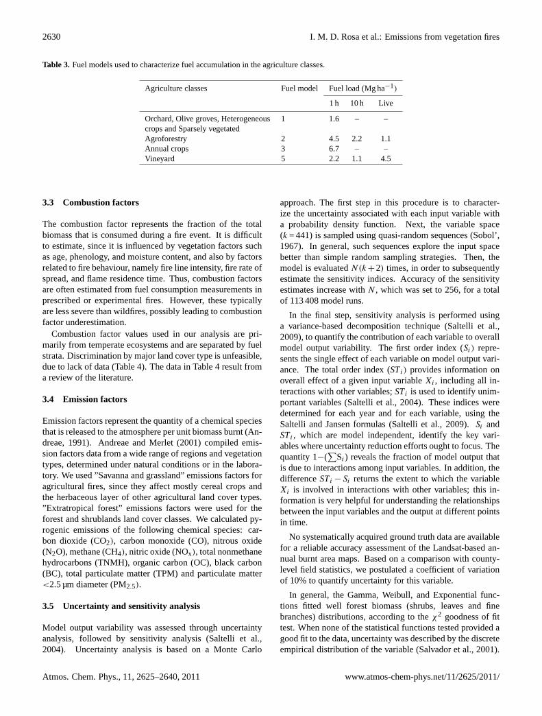
Wildfires affect a variety of agricultural crops, namely vine-yards, olive groves, and rain fed cereal crops. However,no data are available on typical fuel loads for these landcover types, during the fire season. Therefore, we allocatedstandard BEHAVE fuel models (Anderson, 1982) to agricul-tural crops, according to the correspondence established byVelez (2000) for Spain (Table 3).



Table 3. Fuel models used to characterize fuel accumulation in the agriculture classes.

Agriculture classes Fuel model Fuel load (Mg ha−1)

1 h 10 h Live

Orchard, Olive groves, Heterogeneous 1 1.6 – –crops and Sparsely vegetatedAgroforestry 2 4.5 2.2 1.1Annual crops 3 6.7 – –Vineyard 5 2.2 1.1 4.5

3.3 Combustion factors

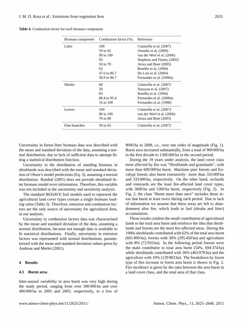
The combustion factor represents the fraction of the totalbiomass that is consumed during a fire event. It is difficultto estimate, since it is influenced by vegetation factors suchas age, phenology, and moisture content, and also by factorsrelated to fire behaviour, namely fire line intensity, fire rate ofspread, and flame residence time. Thus, combustion factorsare often estimated from fuel consumption measurements inprescribed or experimental fires. However, these typicallyare less severe than wildfires, possibly leading to combustionfactor underestimation.

Combustion factor values used in our analysis are pri-marily from temperate ecosystems and are separated by fuelstrata. Discrimination by major land cover type is unfeasible,due to lack of data (Table 4). The data in Table 4 result froma review of the literature.

3.4 Emission factors

Emission factors represent the quantity of a chemical speciesthat is released to the atmosphere per unit biomass burnt (An-dreae, 1991). Andreae and Merlet (2001) compiled emis-sion factors data from a wide range of regions and vegetationtypes, determined under natural conditions or in the labora-tory. We used ”Savanna and grassland” emissions factors foragricultural fires, since they affect mostly cereal crops andthe herbaceous layer of other agricultural land cover types.”Extratropical forest” emissions factors were used for theforest and shrublands land cover classes. We calculated py-rogenic emissions of the following chemical species: car-bon dioxide (CO2), carbon monoxide (CO), nitrous oxide(N2O), methane (CH4), nitric oxide (NOx), total nonmethanehydrocarbons (TNMH), organic carbon (OC), black carbon(BC), total particulate matter (TPM) and particulate matter<2.5 µm diameter (PM2.5).

3.5 Uncertainty and sensitivity analysis

Model output variability was assessed through uncertaintyanalysis, followed by sensitivity analysis (Saltelli et al.,2004). Uncertainty analysis is based on a Monte Carlo

approach. The first step in this procedure is to character-ize the uncertainty associated with each input variable witha probability density function. Next, the variable space(k = 441) is sampled using quasi-random sequences (Sobol’,1967). In general, such sequences explore the input spacebetter than simple random sampling strategies. Then, themodel is evaluatedN(k+2) times, in order to subsequentlyestimate the sensitivity indices. Accuracy of the sensitivityestimates increase withN , which was set to 256, for a totalof 113 408 model runs.

In the final step, sensitivity analysis is performed usinga variance-based decomposition technique (Saltelli et al.,2009), to quantify the contribution of each variable to overallmodel output variability. The first order index (Si) repre-sents the single effect of each variable on model output vari-ance. The total order index (STi) provides information onoverall effect of a given input variableXi , including all in-teractions with other variables;STi is used to identify unim-portant variables (Saltelli et al., 2004). These indices weredetermined for each year and for each variable, using theSaltelli and Jansen formulas (Saltelli et al., 2009).Si andSTi , which are model independent, identify the key vari-ables where uncertainty reduction efforts ought to focus. Thequantity 1−(

∑Si) reveals the fraction of model output that

is due to interactions among input variables. In addition, thedifferenceSTi −Si returns the extent to which the variableXi is involved in interactions with other variables; this in-formation is very helpful for understanding the relationshipsbetween the input variables and the output at different pointsin time.

No systematically acquired ground truth data are availablefor a reliable accuracy assessment of the Landsat-based an-nual burnt area maps. Based on a comparison with county-level field statistics, we postulated a coefficient of variationof 10% to quantify uncertainty for this variable.

In general, the Gamma, Weibull, and Exponential func-tions fitted well forest biomass (shrubs, leaves and finebranches) distributions, according to theχ2 goodness of fittest. When none of the statistical functions tested provided agood fit to the data, uncertainty was described by the discreteempirical distribution of the variable (Salvador et al., 2001).



Table 4. Combustion factor for each biomass component.

Biomass component Combustion factor (%) Reference

Litter 100 Cinnirella et al. (2007)59 to 92 Ormeno et al. (2009)90 to 100 van der Werf et al. (2006)93 Stephens and Finney (2002)50 to 70 Arora and Boer (2005)63 Botelho et al. (1994)47.6 to 86.7 De Luis et al. (2004)58.9 to 86.7 Fernandes et al. (2000a)

Shrubs 60 Cinnirella et al. (2007)50 Narayan et al. (2007)83 Botelho et al. (1994)88.4 to 95.4 Fernandes et al. (2000a)16 to 100 Fernandes et al. (1998)

Leaves 100 Cinnirella et al. (2007)80 to 100 van der Werf et al. (2006)70 to 80 Arora and Boer (2005)

Fine branches 50 to 65 Cinnirella et al. (2007)

Uncertainty in forest litter biomass data was described withthe mean and standard deviation of the data, assuming a nor-mal distribution; due to lack of sufficient data to attempt fit-ting a statistical distribution function.

Uncertainty in the distribution of standing biomass inshrublands was described with the mean and standard devia-tion of Olson’s model predictions (Eq. 3), assuming a normaldistribution. Rambal (2001) does not provide shrubland lit-ter biomass model error information. Therefore, this variablewas not included in the uncertainty and sensitivity analysis.

The standard BEHAVE fuel models used to represent theagricultural land cover types contain a single biomass load-ing value (Table 3). Therefore, emission and combustion fac-tors are the only source of uncertainty for agricultural fires,in our analysis.

Uncertainty in combustion factors data was characterisedby the mean and standard deviation of the data, assuming anormal distribution, because not enough data is available tofit statistical distributions. Finally, uncertainty in emissionfactors was represented with normal distributions, parame-terised with the mean and standard deviation values given byAndreae and Merlet (2001).

4 Results

4.1 Burnt area

Inter-annual variability in area burnt was very high duringthe study period, ranging from over 300 000 ha and over400 000 ha in 2005 and 2003, respectively, to a low of

9000 ha in 2008, i.e., over one order of magnitude (Fig. 1).Burnt area increased substantially, from a total of 900 000 hain the first decade to 1300 000 ha in the second period.

During the 19 years under analysis, the land cover classmost affected by fire was “Shrublands and grasslands”, withmore than 600 000 ha burnt. Maritime pine forests and Eu-calypt forests also burnt extensively: more than 335 000 haand 333 000 ha, respectively. On the other hand, orchardsand vineyards are the least fire-affected land cover types,with 3600 ha and 5300 ha burnt, respectively (Fig. 2). InFig. 2, the class “Burnt more than once” includes those ar-eas that burnt at least twice during each period. Due to lackof information we assume that these areas are left to aban-donment after fire, which leads to fuel (shrubs and litter)accumulation.

These results confirm the small contribution of agriculturallands to the total area burnt and reinforce the idea that shrub-lands and forests are the most fire-affected areas. During the1990s shrublands contributed with 62% of the total area burnt(601 800 ha), forests with 30% (295 450 ha) and agriculturewith 8% (72 910 ha). In the following period forests werethe main contributor to total area burnt (54%, 694 374 ha)while shrublands contributed with 36% (463 878 ha) and theagriculture with 10% (129 803 ha). The breakdown by foresttype of this increase in forest area burnt is shown in Fig. 2.Fire incidence is given by the ratio between the area burnt ina land cover class, and the total area of that class.



Fig. 1. Total burnt area in Portugal between 1990 and 2008.

Fig. 2. Total burnt area and fire incidence by land cover class be-tween 1990 and 2008.

4.2 Biomass

4.2.1 Forests

The median was used to quantify the biomass of shrubs, andof tree leaves and fine branches due to the strong bias ofthe data towards a higher frequency of low biomass values.Mean values are also given (in brackets) to facilitate compar-ison with results from previous research.

Forest understory shrub biomass displayed a wide rangeof values, varying from a median of 0 and 0.14 Mg ha−1

(1.8 and 3.09 Mg ha−1) for Holm oak and Cork oak in ev-ergreen oak woodlands, to a maximum of 4.45 Mg ha−1

(8.24 Mg ha−1) in Maritime pine stands. Similar resultswere obtained for tree leaf and fine branch biomass. Thelowest median tree leaf values were also obtained forevergreen oak woodlands, varying between 0.21 Mg ha−1

Fig. 3. Biomass accumulation (Mg ha−1) in each forest class.

and 0.32 Mg ha−1 (0.25 and 0.41 Mg ha−1) for Holm oakand Cork oak, respectively. For the fine branch biomassthe values obtained for these woodlands were 0.35 and0.54 Mg ha−1 (0.42 and 0.7 Mg ha−1) for Holm oak andCork oak, respectively. The highest of all leaf medianbiomass values were obtained for “other conifer forests”,with 4.74 Mg ha−1 (5.06 Mg ha−1), while Umbrella pineforests displayed the highest median fine branch biomass,with 6.20 Mg ha−1 (7.61 Mg ha−1).

Figure 3 shows mean biomass accumulation in each for-est class, by biomass component. The difference in crownbiomass values between the evergreen oaks and the otherspecies is due to stand density differences. Evergreen oakwoodlands in Portugal typically have very low tree density.

4.2.2 Shrublands

Parameter estimation for Olson’s equation yielded the shrub-land biomass accumulation model:

Wshb= 18.86(1−e−0.23t

)(7)

where Wshb (Mg ha−1) is the total aboveground shrubbiomass andt is the stand age, in years. The root meansquare error of the model is 8 Mg ha−1, which is ratherhigh, considering the mean biomass of the original data(13 Mg ha−1). Therefore, this variable will have a signifi-cant uncertainty attached. Table 5 shows the 95% confidenceintervals for the model estimated parameters.

Mean patch age estimated for “Shrublands and grasslands”was 30 years, resulting in estimates of 3.40 Mg ha−1and18.84 Mg ha−1 for shrubland litter and abovegroundbiomass, respectively. The corresponding estimates for theareas that burnt at least twice during the period under anal-ysis were 1.21 Mg ha−1 to 2.68 Mg ha−1 and 3.86 Mg ha−1

to 16.46 Mg ha−1for shrub litter and aboveground biomass,respectively.



Table 5. 95% confidence interval of the parameters estimatedmean value.

Parameter Mean Lower limit Upper limit

a 18.86 17.12 20.60b 0.23 0.17 0.29


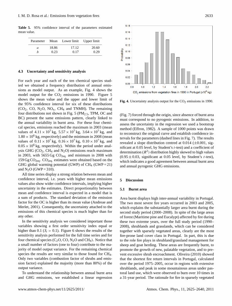
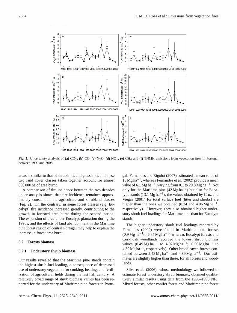
For each year and each of the ten chemical species stud-ied we obtained a frequency distribution of annual emis-sions as model output. As an example, Fig. 4 shows themodel output for the CO2 emissions in 1990. Figure 5shows the mean value and the upper and lower limit ofthe 95% confidence interval for six of these distributions(CO2, CO, N2O, NOx, CH4 and TNMH). The remainingfour distributions not shown in Fig. 5 (PM2.5, TPM, OC andBC) present the same emissions pattern, clearly linked tothe annual variability in burnt area. For these four chemi-cal species, emissions reached the maximum in 2003 (meanvalues of 4.11× 107 kg, 5.57× 107 kg, 3.64× 107 kg, and1.80× 106 kg, respectively) and the minimum in 2008 (meanvalues of 0.11× 107 kg, 0.16× 107 kg, 0.10× 107 kg, and0.05× 106 kg, respectively). Within the period under anal-ysis GHG (CO2, CH4 and N2O) emissions reach maximumin 2003, with 5655 Gg CO2eq. and minimum in 2008 with159 Gg CO2eq. CO2eq. estimates were obtained based on theGHG global warming potential (GWP) of CH4 (GWP = 21)and N2O (GWP = 310).

All time series display a strong relation between mean andconfidence interval, i.e. years with higher mean emissionsvalues also show wider confidence intervals, implying higheruncertainty in the estimates. Direct proportionality betweenmean and confidence interval is expected in a model that isa sum of products. The standard deviation of the emissionfactor for the OC is higher than its mean value (Andreae andMerlet, 2001). Consequently, the uncertainty attached to theemissions of this chemical species is much higher than forany other.

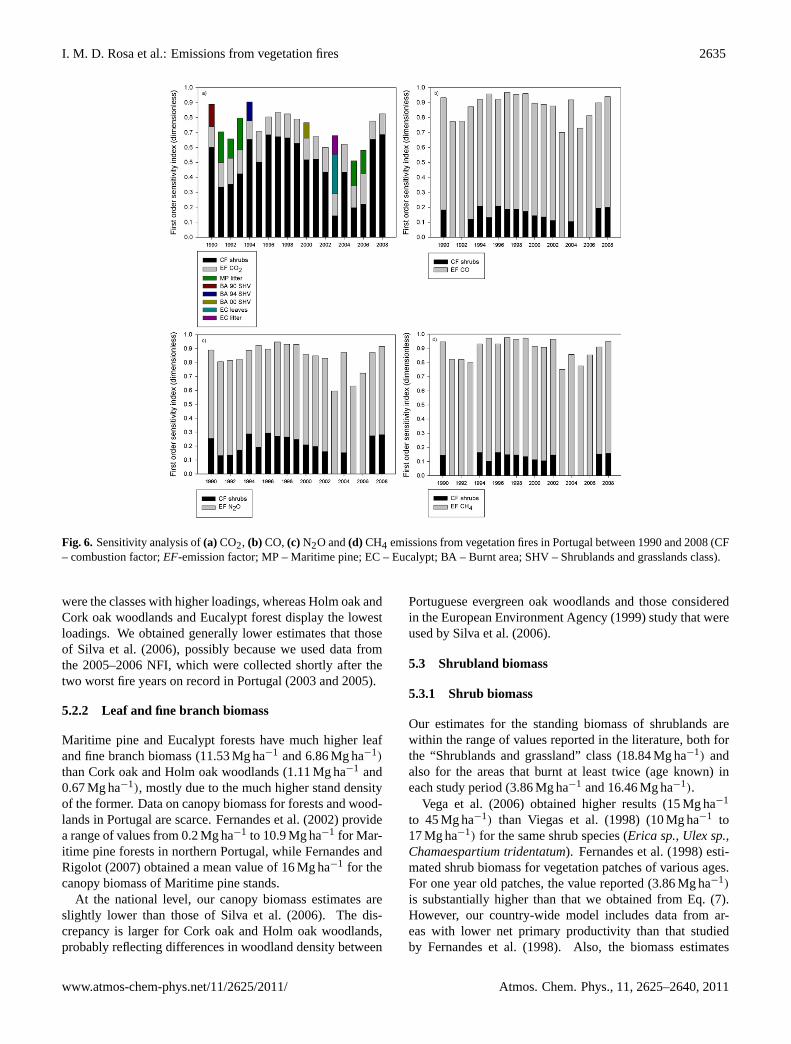
In the sensitivity analysis we considered important thosevariables showing a first order sensitivity index equal orhigher than 0.1 (Si > 0.1). Figure 6 shows the results of thesensitivity analysis performed for the full time series and forfour chemical species (C2O, CO, N2O and CH4). Notice thata small number of factors (one to four) contribute to the ma-jority of model output variance. For the remaining chemicalspecies the results are very similar to those found for CH4.Only two variables (combustion factor of shrubs and emis-sion factor) explained the majority (more than 80%) of theoutput variance.

To understand the relationship between annual burnt areaand GHG emissions, we established a linear regression

Fig. 4. Uncertainty analysis output for the CO2 emissions in 1990.

(Fig. 7) forced through the origin, since absence of burnt areamust correspond to no pyrogenic emissions. In addition, toassess the uncertainty in the regression we used a bootstrapmethod (Effron, 1982). A sample of 1000 points was drawnto reconstruct the original curve and establish confidence in-tervals for the parameters (dashed lines in Fig. 7). The resultsrevealed a slope distribution centred at 0.014 (±0.001, sig-nificant at 0.05 level, by Student’st-test) and a coefficient ofdetermination (R2) distribution highly skewed to high values(0.95± 0.03, significant at 0.05 level, by Student’st-test),which indicates a good agreement between annual burnt areaand annual pyrogenic GHG emissions.

5 Discussion

5.1 Burnt area

Area burnt displays high inter-annual variability in Portugal.The two most severe fire years occurred in 2003 and 2005,which explains the substantially larger area burnt during thesecond study period (2000–2008). In spite of the large areasof forest (Maritime pine and Eucalypt) affected by fire duringthese two extreme years, over the full study period (1990–2008), shrublands and grasslands, which can be consideredtogether with sparsely vegetated areas, clearly are the mostfire-prone land cover class in Portugal. In part, this is dueto the role fire plays in shrubland/grassland management forsheep and goat herding. These areas are frequently burnt, topromote the growth of new, palatable vegetation, and to pre-vent excessive shrub encroachment. Oliveira (2010) showedthat the shortest fire return intervals in Portugal, calculatedover the period 1975–2005, occur in regions with extensiveshrublands, and peak in some mountainous areas under pas-toral land use, which were observed to burn over 10 times ina 31-year period. The rationale for fire in sparsely vegetated



Fig. 5. Uncertainty analysis of(a) CO2, (b) CO, (c) N2O, (d) NOx, (e) CH4 and (f) TNMH emissions from vegetation fires in Portugalbetween 1990 and 2008.

areas is similar to that of shrublands and grasslands and thesetwo land cover classes taken together account for almost800 000 ha of area burnt.

A comparison of fire incidence between the two decadesunder analysis shows that fire incidence remained approx-imately constant in the agriculture and shrubland classes(Fig. 2). On the contrary, in some forest classes (e.g. Eu-calypt) fire incidence increased greatly, contributing to thegrowth in forested area burnt during the second period.The expansion of area under Eucalypt plantation during the1990s, and the effects of land abandonment in the Maritimepine forest region of central Portugal may help to explain theincrease in forest area burnt.

5.2 Forests biomass

5.2.1 Understory shrub biomass

Our results revealed that the Maritime pine stands containthe highest shrub fuel loading, a consequence of decreaseduse of understory vegetation for cooking, heating, and fertil-ization of agricultural fields during the last half century. Arelatively broad range of shrub biomass values has been re-ported for the understory of Maritime pine forests in Portu-

gal. Fernandes and Rigolot (2007) estimated a mean value of15 Mg ha−1, whereas Fernandes et al. (2002) provide a meanvalue of 6.1 Mg ha−1, varying from 0.1 to 20.8 Mg ha−1. Notonly for the Maritime pine (42 Mg ha−1) but also for Euca-lypt stands (13.1 Mg ha−1), the values obtained by Cruz andViegas (2001) for total surface fuel (litter and shrubs) arehigher than the ones we obtained (8.24 and 4.96 Mg ha−1,respectively). However, they also obtained higher under-story shrub fuel loadings for Maritime pine than for Eucalyptstands.

The higher understory shrub fuel loadings reported byFernandes (2009) were found in Maritime pine forests(0.9 Mg ha−1to 6.35 Mg ha−1) whereas Eucalypt forests andCork oak woodlands recorded the lowest shrub biomassvalues (0.49 Mg ha−1 to 4.02 Mg ha−1; 0.56 Mg ha−1 to4.39 Mg ha−1, respectively). Other broadleaved forests con-tained between 2.48 Mg ha−1 and 4.89 Mg ha−1. Our esti-mates are slightly higher than these, for all forests and wood-lands.

Silva et al. (2006), whose methodology we followed toestimate forest understory shrub biomass, obtained qualita-tively similar results using data from the 1995–1998 NFI.Mixed forests, other conifer forest and Maritime pine forest



Fig. 6. Sensitivity analysis of(a) CO2, (b) CO,(c) N2O and(d) CH4 emissions from vegetation fires in Portugal between 1990 and 2008 (CF– combustion factor;EF-emission factor; MP – Maritime pine; EC – Eucalypt; BA – Burnt area; SHV – Shrublands and grasslands class).

were the classes with higher loadings, whereas Holm oak andCork oak woodlands and Eucalypt forest display the lowestloadings. We obtained generally lower estimates that thoseof Silva et al. (2006), possibly because we used data fromthe 2005–2006 NFI, which were collected shortly after thetwo worst fire years on record in Portugal (2003 and 2005).

5.2.2 Leaf and fine branch biomass

Maritime pine and Eucalypt forests have much higher leafand fine branch biomass (11.53 Mg ha−1 and 6.86 Mg ha−1)

than Cork oak and Holm oak woodlands (1.11 Mg ha−1 and0.67 Mg ha−1), mostly due to the much higher stand densityof the former. Data on canopy biomass for forests and wood-lands in Portugal are scarce. Fernandes et al. (2002) providea range of values from 0.2 Mg ha−1 to 10.9 Mg ha−1 for Mar-itime pine forests in northern Portugal, while Fernandes andRigolot (2007) obtained a mean value of 16 Mg ha−1 for thecanopy biomass of Maritime pine stands.

At the national level, our canopy biomass estimates areslightly lower than those of Silva et al. (2006). The dis-crepancy is larger for Cork oak and Holm oak woodlands,probably reflecting differences in woodland density between

Portuguese evergreen oak woodlands and those consideredin the European Environment Agency (1999) study that wereused by Silva et al. (2006).

5.3 Shrubland biomass

5.3.1 Shrub biomass

Our estimates for the standing biomass of shrublands arewithin the range of values reported in the literature, both forthe “Shrublands and grassland” class (18.84 Mg ha−1) andalso for the areas that burnt at least twice (age known) ineach study period (3.86 Mg ha−1 and 16.46 Mg ha−1).

Vega et al. (2006) obtained higher results (15 Mg ha−1

to 45 Mg ha−1) than Viegas et al. (1998) (10 Mg ha−1 to17 Mg ha−1) for the same shrub species (Erica sp., Ulex sp.,Chamaespartium tridentatum). Fernandes et al. (1998) esti-mated shrub biomass for vegetation patches of various ages.For one year old patches, the value reported (3.86 Mg ha−1)

is substantially higher than that we obtained from Eq. (7).However, our country-wide model includes data from ar-eas with lower net primary productivity than that studiedby Fernandes et al. (1998). Also, the biomass estimates



obtained by Fernandes et al. (2000a) in the north-eastern Por-tugal for 5-year old shrublands are lower those predicted byEq. (7). Our own estimates, although higher than those ofSilva et al. (2006), are closer to values previously reportedfor Portugal.

5.3.2 Litter biomass

Our results for shrubland litter biomass are within the rangeof values reported for Mediterranean countries. Dimi-trakopoulos (2002) estimated loadings of 0.7 Mg ha−1 to3.4 Mg ha−1 for shrublands in Greece. In Turkey, Saglamet al. (2008) reported shrubland litter values of up to12.4 Mg ha−1, with a mean value of 4.4 Mg ha−1. InSpain, De Luis et al. (2004) obtained higher values thanours, for 12-year old shrubland communities (9.24 Mg ha−1,18.17 Mg ha−1, and 18.98 Mg ha−1). Our calculations oflitter accumulation have a direct, deterministic relation-ship with shrubland biomass (Eq. 7). Since our estimatesof shrubland biomass were higher than those of Silva etal. (2006), our litter estimates necessarily exceed theirs.


Figure 5 summarises model output uncertainty. Resultsof the uncertainty analysis for the entire time series re-veal a very high inter-annual variability, which reflects an-nual area burnt. Within this large annual variability, 2003was the year with the highest pyrogenic GHG and aerosolsemissions. CO2 was the gas with larger quantities emit-ted (5083± 1,703 Gg, 95% C.I.,n = 256) (Fig. 5a). How-ever, significant amounts of N2O and CH4 were also released(259± 140 Gg and 313± 233 Gg CO2eq., 95% C.I.,n = 256,respectively) (Fig. 5c and e). Pyrogenic emissions werelowest in 2008 with only 143± 46 Gg CO2, 9± 6 Gg CO2eq.CH4 and 7± 4 Gg CO2eq. N2O (95% C.I.,n = 256) emitted(Figs. 5a, c and e). Our estimates are highly correlated (Pear-son’s correlation (r), all significant at 0.01 level) with thewildfires’ GHG emissions reported by the European Environ-ment Agency (EEA) for the same period in Portugal (Pereiraet al., 2009b). The burnt area estimates are highly correlated(r = 0.95), as well as the GHG (r = 0.91), CO2 (r = 0.91),CH4 (r = 0.99) and N2O emissions (r = 0.99).

Both methods revealed 2003 and 2008 as the yearswith higher and lower emissions, respectively. However,our estimates are much more conservative (5655versus11 289 Gg CO2eq. in 2003), despite the fact that our burntarea estimates are higher (440 025versus286 000 ha). Thesedifferences arise mainly from significant discrepancies be-tween CO2 pyrogenic emissions estimates. Contrarily to ourstudy, EEA also account for indirect carbon losses, such asthe natural decay of dead organic matter following fires, aswell as harvesting emissions, which account for the loss ofthe entire dead tree at the time of fire (Pereira et al., 2009b).This can lead to an overestimation since it includes leaves,

branches, wood, bark and roots. On the contrary, as men-tioned above, we assume that in a typical fire only leaves andsmall branches are consumed, which can lead to some under-estimation in the case of severe wildfires.

The complexity of the sensitivity analysis performed inthis study is due to the large number (a total of 441) of vari-ables considered. However, most of these variables haveSi

andSTi values close to zero, meaning they have very smallimpact in the output variance and can be held constant. Inter-actions between variables play hardly any role in determiningmodel output variability. Only a small number of factors in-teract (STi > Si), and they do it at a very weak levels. Thisis true for every chemical species except CO2, which dis-plays stronger interactions between variables (Fig. 6a). CO2emissions are orders of magnitude larger than those of otherspecies, and since uncertainties are directly proportional toemissions (due to the multiplicative model used); this proba-bly leads to the existence of more interactions between vari-ables. The same argument can explain why in the years 2003and 2005, which were the years with the highest amount ofarea burnt, there are more interactions than in any other yearwithin the time series (Fig. 6). Therefore, the occurrence andmagnitude of interactions are evidently related to the exis-tence of variables with larger uncertainty range.

Sensitivity analysis for chemical species with a positiveemission factor coefficient of variation (for example, PM2.5,OC and TNMH) revealed the large influence of this variableon model output. In these cases, the single effect of this vari-able always accounted for more than 80% of model outputvariance.

The sensitivity analysis identified emission factors forforests and shrublands, and the combustion factor of shrub-lands as the variables with the largest impact on model outputvariance. Importance of the latter variable possibly reflectsthe large extent of shrubland area burnt. The single effects ofthese two variables add to roughly 80–90% of the total modeloutput variance, meaning that the effect of interactions be-tween variables is quite low (10–20% of the total variance).These results were similar for every year and every chemicalspecies under analysis (except for CO2). Therefore, it is veryimportant to reduce uncertainties attached to these variables,in order to lower model output variance.

Combustion factors intrinsically are very variable, due totheir strong dependence on fuel moisture and fire behaviour.A shortage of data on this variable for wildfires in Portu-gal further enhances associated uncertainty. It may be possi-ble to model combustion completeness as a function of a fireweather index (Amiro et al., 2001), thus obtaining more ac-curate estimates, but natural variability is expected to remainhigh. Emission factors proved to be the variable to whichmodel outputs are most sensitive. Thus, it ought to be a pri-ority target for uncertainty reduction in emissions estimation.

Miranda et al. (2008) published emission estimates for arange of land cover types in Portugal, but only mean valueswere provided. Pyrogenic emissions obtained in the present



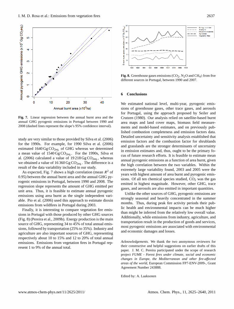
Fig. 7. Linear regression between the annual burnt area and theannual GHG pyrogenic emissions in Portugal between 1990 and2008 (dashed lines represent the slope’s 95% confidence interval).

study are very similar to those provided by Silva et al. (2006)for the 1990s. For example, for 1990 Silva et al. (2006)estimated 1640 Gg CO2eq. of GHG whereas we determineda mean value of 1540 Gg CO2eq.. For the 1990s, Silva etal. (2006) calculated a value of 19 218 Gg CO2eq., whereaswe obtained a value of 16 360 Gg CO2eq.. The difference is aresult of the data variability included in our study.

As expected, Fig. 7 shows a high correlation (meanR2 of0.95) between the annual burnt area and the annual GHG py-rogenic emissions in Portugal, between 1990 and 2008. Theregression slope represents the amount of GHG emitted perunit area. Thus, it is feasible to estimate annual pyrogenicemissions using area burnt as the single independent vari-able. Pio et al. (2006) used this approach to estimate dioxinemissions from wildfires in Portugal during 2003.

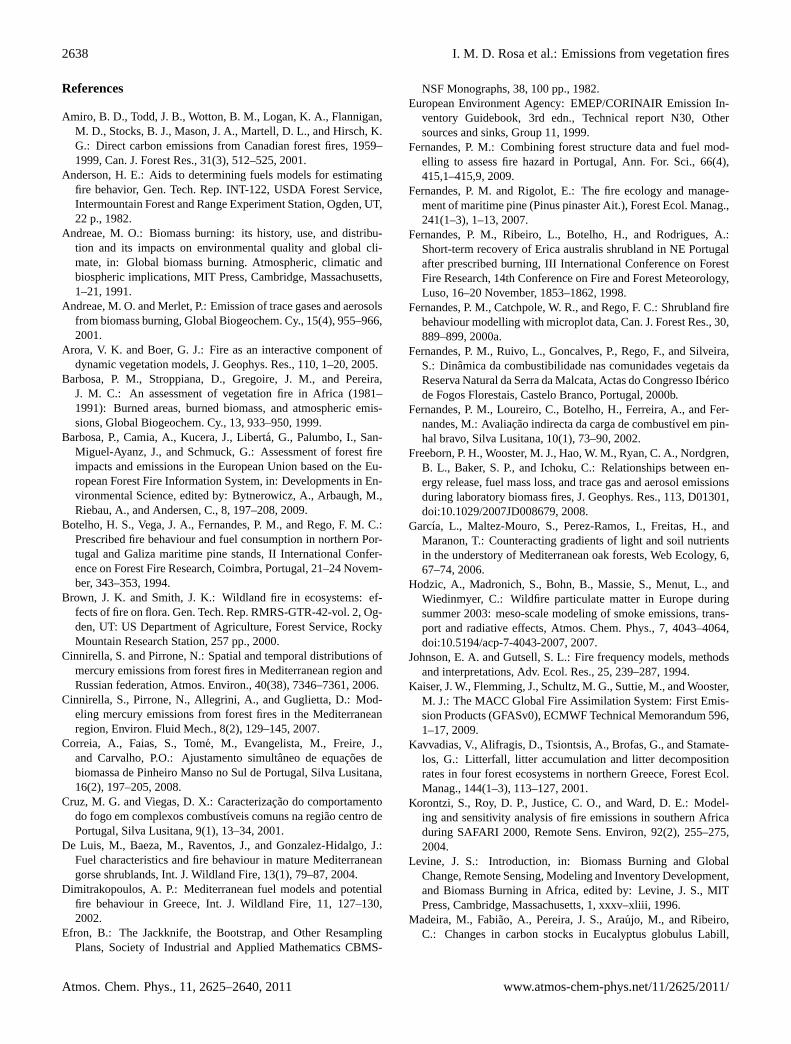
Finally, it is interesting to compare vegetation fire emis-sions in Portugal with those produced by other GHG sources(Fig. 8) (Pereira et al., 2009b). Energy production is the mainsource of GHG, representing 34 to 45% of total annual emis-sions, followed by transportation (25% to 35%). Industry andagriculture are also important sources of GHG, representingrespectively about 10 to 15% and 12 to 20% of total annualemissions. Emissions from vegetation fires in Portugal rep-resent 1 to 9% of the annual total.

Fig. 8. Greenhouse gases emissions (CO2, N2O and CH4) from fivedifferent sources in Portugal, between 1990 and 2007.

6 Conclusions

We estimated national level, multi-year, pyrogenic emis-sions of greenhouse gases, other trace gases, and aerosolsfor Portugal, using the approach proposed by Seiler andCrutzen (1980). Our analysis relied on satellite-based burntarea maps and land cover maps, biomass field measure-ments and model-based estimates, and on previously pub-lished combustion completeness and emission factors data.Detailed uncertainty and sensitivity analysis established thatemission factors and the combustion factor for shrublandsand grasslands are the stronger determinants of uncertaintyin emission estimates and, thus, ought to be the primary fo-cus of future research efforts. It is feasible to estimate meanannual pyrogenic emissions as a function of area burnt, giventhe high correlation between the two variables. Within theextremely large variability found, 2003 and 2005 were theyears with highest amount of area burnt and pyrogenic emis-sions. Of all ten chemical species studied, CO2 was the gasemitted in highest magnitude. However, other GHG, tracegases, and aerosols are also emitted in important quantities.

Unlike the other sources of GHG, pyrogenic emissions arestrongly seasonal and heavily concentrated in the summermonths. Thus, during peak fire activity periods their pub-lic health and environmental impacts can be much higherthan might be inferred from the relatively low overall value.Additionally, while emissions from industry, agriculture, andtransportation result in the production of goods and services,most pyrogenic emissions are associated with environmentaland economic damages and losses.

Acknowledgements.We thank the two anonymous reviewers fortheir constructive and helpful suggestions on earlier drafts of thispaper. J. M. C. Pereira participated under the scope of researchproject FUME - Forest fires under climate, social and economicchanges in Europe, the Mediterranean and other fire-affectedareas of the world, European Commission FP7-ENV-2009-, GrantAgreement Number 243888.

Edited by: A. Laaksonen



References

Amiro, B. D., Todd, J. B., Wotton, B. M., Logan, K. A., Flannigan,M. D., Stocks, B. J., Mason, J. A., Martell, D. L., and Hirsch, K.G.: Direct carbon emissions from Canadian forest fires, 1959–1999, Can. J. Forest Res., 31(3), 512–525, 2001.

Anderson, H. E.: Aids to determining fuels models for estimatingfire behavior, Gen. Tech. Rep. INT-122, USDA Forest Service,Intermountain Forest and Range Experiment Station, Ogden, UT,22 p., 1982.

Andreae, M. O.: Biomass burning: its history, use, and distribu-tion and its impacts on environmental quality and global cli-mate, in: Global biomass burning. Atmospheric, climatic andbiospheric implications, MIT Press, Cambridge, Massachusetts,1–21, 1991.

Andreae, M. O. and Merlet, P.: Emission of trace gases and aerosolsfrom biomass burning, Global Biogeochem. Cy., 15(4), 955–966,2001.

Arora, V. K. and Boer, G. J.: Fire as an interactive component ofdynamic vegetation models, J. Geophys. Res., 110, 1–20, 2005.

Barbosa, P. M., Stroppiana, D., Gregoire, J. M., and Pereira,J. M. C.: An assessment of vegetation fire in Africa (1981–1991): Burned areas, burned biomass, and atmospheric emis-sions, Global Biogeochem. Cy., 13, 933–950, 1999.

Barbosa, P., Camia, A., Kucera, J., Liberta, G., Palumbo, I., San-Miguel-Ayanz, J., and Schmuck, G.: Assessment of forest fireimpacts and emissions in the European Union based on the Eu-ropean Forest Fire Information System, in: Developments in En-vironmental Science, edited by: Bytnerowicz, A., Arbaugh, M.,Riebau, A., and Andersen, C., 8, 197–208, 2009.

Botelho, H. S., Vega, J. A., Fernandes, P. M., and Rego, F. M. C.:Prescribed fire behaviour and fuel consumption in northern Por-tugal and Galiza maritime pine stands, II International Confer-ence on Forest Fire Research, Coimbra, Portugal, 21–24 Novem-ber, 343–353, 1994.

Brown, J. K. and Smith, J. K.: Wildland fire in ecosystems: ef-fects of fire on flora. Gen. Tech. Rep. RMRS-GTR-42-vol. 2, Og-den, UT: US Department of Agriculture, Forest Service, RockyMountain Research Station, 257 pp., 2000.

Cinnirella, S. and Pirrone, N.: Spatial and temporal distributions ofmercury emissions from forest fires in Mediterranean region andRussian federation, Atmos. Environ., 40(38), 7346–7361, 2006.

Cinnirella, S., Pirrone, N., Allegrini, A., and Guglietta, D.: Mod-eling mercury emissions from forest fires in the Mediterraneanregion, Environ. Fluid Mech., 8(2), 129–145, 2007.

Correia, A., Faias, S., Tome, M., Evangelista, M., Freire, J.,and Carvalho, P.O.: Ajustamento simultaneo de equacoes debiomassa de Pinheiro Manso no Sul de Portugal, Silva Lusitana,16(2), 197–205, 2008.

Cruz, M. G. and Viegas, D. X.: Caracterizacao do comportamentodo fogo em complexos combustıveis comuns na regiao centro dePortugal, Silva Lusitana, 9(1), 13–34, 2001.

De Luis, M., Baeza, M., Raventos, J., and Gonzalez-Hidalgo, J.:Fuel characteristics and fire behaviour in mature Mediterraneangorse shrublands, Int. J. Wildland Fire, 13(1), 79–87, 2004.

Dimitrakopoulos, A. P.: Mediterranean fuel models and potentialfire behaviour in Greece, Int. J. Wildland Fire, 11, 127–130,2002.

Efron, B.: The Jackknife, the Bootstrap, and Other ResamplingPlans, Society of Industrial and Applied Mathematics CBMS-

NSF Monographs, 38, 100 pp., 1982.European Environment Agency: EMEP/CORINAIR Emission In-

ventory Guidebook, 3rd edn., Technical report N30, Othersources and sinks, Group 11, 1999.

Fernandes, P. M.: Combining forest structure data and fuel mod-elling to assess fire hazard in Portugal, Ann. For. Sci., 66(4),415,1–415,9, 2009.

Fernandes, P. M. and Rigolot, E.: The fire ecology and manage-ment of maritime pine (Pinus pinaster Ait.), Forest Ecol. Manag.,241(1–3), 1–13, 2007.

Fernandes, P. M., Ribeiro, L., Botelho, H., and Rodrigues, A.:Short-term recovery of Erica australis shrubland in NE Portugalafter prescribed burning, III International Conference on ForestFire Research, 14th Conference on Fire and Forest Meteorology,Luso, 16–20 November, 1853–1862, 1998.

Fernandes, P. M., Catchpole, W. R., and Rego, F. C.: Shrubland firebehaviour modelling with microplot data, Can. J. Forest Res., 30,889–899, 2000a.

Fernandes, P. M., Ruivo, L., Goncalves, P., Rego, F., and Silveira,S.: Dinamica da combustibilidade nas comunidades vegetais daReserva Natural da Serra da Malcata, Actas do Congresso Ibericode Fogos Florestais, Castelo Branco, Portugal, 2000b.

Fernandes, P. M., Loureiro, C., Botelho, H., Ferreira, A., and Fer-nandes, M.: Avaliacao indirecta da carga de combustıvel em pin-hal bravo, Silva Lusitana, 10(1), 73–90, 2002.

Freeborn, P. H., Wooster, M. J., Hao, W. M., Ryan, C. A., Nordgren,B. L., Baker, S. P., and Ichoku, C.: Relationships between en-ergy release, fuel mass loss, and trace gas and aerosol emissionsduring laboratory biomass fires, J. Geophys. Res., 113, D01301,doi:10.1029/2007JD008679, 2008.

Garcıa, L., Maltez-Mouro, S., Perez-Ramos, I., Freitas, H., andMaranon, T.: Counteracting gradients of light and soil nutrientsin the understory of Mediterranean oak forests, Web Ecology, 6,67–74, 2006.

Hodzic, A., Madronich, S., Bohn, B., Massie, S., Menut, L., andWiedinmyer, C.: Wildfire particulate matter in Europe duringsummer 2003: meso-scale modeling of smoke emissions, trans-port and radiative effects, Atmos. Chem. Phys., 7, 4043–4064,doi:10.5194/acp-7-4043-2007, 2007.

Johnson, E. A. and Gutsell, S. L.: Fire frequency models, methodsand interpretations, Adv. Ecol. Res., 25, 239–287, 1994.

Kaiser, J. W., Flemming, J., Schultz, M. G., Suttie, M., and Wooster,M. J.: The MACC Global Fire Assimilation System: First Emis-sion Products (GFASv0), ECMWF Technical Memorandum 596,1–17, 2009.

Kavvadias, V., Alifragis, D., Tsiontsis, A., Brofas, G., and Stamate-los, G.: Litterfall, litter accumulation and litter decompositionrates in four forest ecosystems in northern Greece, Forest Ecol.Manag., 144(1–3), 113–127, 2001.

Korontzi, S., Roy, D. P., Justice, C. O., and Ward, D. E.: Model-ing and sensitivity analysis of fire emissions in southern Africaduring SAFARI 2000, Remote Sens. Environ, 92(2), 255–275,2004.

Levine, J. S.: Introduction, in: Biomass Burning and GlobalChange, Remote Sensing, Modeling and Inventory Development,and Biomass Burning in Africa, edited by: Levine, J. S., MITPress, Cambridge, Massachusetts, 1, xxxv–xliii, 1996.

Madeira, M., Fabiao, A., Pereira, J. S., Araujo, M., and Ribeiro,C.: Changes in carbon stocks in Eucalyptus globulus Labill,


http://dx.doi.org/10.5194/acp-7-4043-2007


plantations induced by different water and nutrient availability,Forest Ecol. Manag., 171(1), 75–85, 2002.

Mather, A. and Pereira, J. M. C.: Transicao florestal e fogo emPortugal, in: Incendios florestais em Portugal: caracterizacao,impactes e prevencao, edited by: Pereira, J. S., Pereira, J. M.C., Rego, F., Silva, J. M. N., and Silva, T. P., ISAPress, Lisboa,257–282, 2006.

Miranda, A. I., Coutinho, M., and Borrego, C.: Forest fire emissionsin Portugal: A contribution to global warming?, Environ. Pollut.,83(1–2), 121–123, 1994.

Miranda, A. I., Monteiro, A., Martins, V., Carvalho, A., Schaap, M.,Builtjes, P., and Borrego, C.: Forest fires impact on air qualityover Portugal, in: NATO/CCMS International Technical Meet-ing on Air Pollution Modeling and its applications, 29, 190–198,edited by: Borrego, C. and Miranda, A. I., Springer, Aveiro, Por-tugal, 2008.

Miranda, A. I., Marchi, E., Ferretti, M., and Millan, M. M.: Forestfires and air quality issues in Southern Europe, in: Developmentsin Environmental Science, edited by: Bytnerowicz, A., Arbaugh,M., Riebau, A., and Andersen, C., 8, 209–231, 2009a.

Miranda, A. I., Borrego, C., Martins, H., Martins, V., Amorim, J. H.,Valente, J., and Carvalho, A.: Forest fire emissions and air pollu-tion in southern Europe, 171–187, in: Earth observation of wild-land fires in Mediterranean ecosystems, edited by: Chuvieco, E.,Springer-Verlag, Berlin, Heidelberg, Germany, 2009b.

Montero, G., Ruiz-Peinado, R., and Munoz, M.: Produccion debiomasa y fijacion de CO2 por los bosques espanoles, INIA, 220,25–36, 2005.

Narayan, C., Fernandes, P. M., van Brusselen, J., and Schuck, A.:Potential for CO2 emissions mitigation in Europe through pre-scribed burning in the context of the Kyoto Protocol, Forest Ecol.Manag., 251(3), 164–173, 2007.

National Forest Authority: 5th National Forest Inventory –Mainland Portugal,http://www.afn.min-agricultura.pt/portal/ifn/relatorio-final-ifn5-florestat-1, 2010.

Oliveira, S. L. J., Pereira, J. M. C., and Carreiras, J. M. B.: Fire fre-quency analysis in Portugal (1975–2005), using satellite-basedburned area maps, Int. J. Wildland Fire, submitted, 2010.

Olson, J. S.: Energy storage and the balance of producers anddecomposers in ecological systems, Ecology, 44(2), 322–331,1963.

Ormeno, E., Cespedes, B., Sanchez, I., Velasco-Garcıa, A., Moreno,J., Fernandez, C., and Baldy, V.: The relationship between ter-penes and flammability of leaf litter, Forest Ecol. Manag., 257(2),471–482, 2009.

Pereira, J. S., Correia, A. V., Correia, A. P., Pereira, J. M. C.,Oliveira, A. C., Freitas, H., Reis, R. M., Branco, M., Caldeira,M. C., Cruz, C. S., Bugalho, M., and Vasconcelos, M. J.: Forestsand biodiversity, Climate Change in Portugal, Scenarios, Impactsand Adaptation Measures, edited by: Santos, F. D., Forbes, K.,and Moita, R., Gradiva, Lisboa, 369–413, 2002.

Pereira, J. M. C. and Santos, M. T. N.: Fire risk and burnt areamapping in Portugal, Direccao Geral das Florestas, Lisboa, 2003.

Pereira, G., Freitas, S. R., Moraes, E. C., Ferreira, N. J.,Shimabukuro, Y. E., Rao, V. B., and Longo, K. M.: Estimatingtrace gas and aerosol emissions over South America: relationshipbetween fire radiative energy released and aerosol optical depthobservations, Atmos. Environ., 43, 6388–6397, 2009a.

Pereira, T. C., Seabra, T., Maciel, H., and Torres, P.: Portuguese na-

tional inventory report on greenhouse gases, 1990–2007, Submit-ted under the United Nations framework convention on climatechange and the Kyoto protocol, Agencia Portuguesa do Ambi-ente, 2009b.

Pio, C. A., Silva, T. P., and Pereira, J. M. C.: Emissoes e impacto naatmosfera, in: Incendios florestais em Portugal: caracterizacao,impactes e prevencao, edited by: Pereira, J. S., Pereira, J. M.C., Rego, F., Silva, J. M. N., and Silva, T. P., ISAPress, Lisboa,165–198, 2006.

Pio, C. A., Legrand, M., Alves, C. A., Oliveira, T., Afonso, J., Ca-seiro, A., Puxbaum, H., Sanchez-Ochoa, A., and Gelencser, A.:Chemical composition of atmospheric aerosols during the 2003summer intense forest fire period, Atmos. Environ., 42, 7530–7543, 2008.

Rambal, S.: Hierarchy and productivity of Mediterranean-typeecosystems, in: Terrestrial global productivity, Academic Press,San Diego, 315–344, 2001.

Saglam, B., Kucuk, O., Bilgili, E., Durmaz, B., and Baysal, I.: Es-timating fuel biomass of some shrub species (Maquis) in Turkey,Turk. J. Agric. For., 32, 349–356, 2008.

Saltelli, A., Tarantola, S., Campolongo, F., and Ratto, M.: Sensi-tivity analysis in practice. A guide to assessing scientific models,John Wiley & Sons Ltd., West Sussex, England, 2004.

Saltelli, A., Annoni, P., Azzini, I., Campolongo, F., Ratto, M., andTarantola, S.: Variance based sensitivity analysis of model out-put, Design and estimator for the total sensitivity index, Comput.Phys. Commun., 2009

Salvador, R., Pinol, J., Tarantola, S., and Pla, E.: Global sensitivityanalysis and scale effects of a fire propagation model used overMediterranean shrublands, Ecol. Model., 136, 175–189, 2001.

Sandberg, D. V., Ottmar, R. D., Peterson, J. L., and Core, J.: Wild-land fire on ecosystems: effects of fire on air, Gen. Tech. Rep.RMRS-GTR-42-vol. 5. Ogden, UT: US Department of Agricul-ture, Forest Service, Rocky Mountain Research Station, 79 pp.,2002.

Scholes, R. J., Ward, D. E., and Justice, C. O.: Emissions of tracegases and aerosol particles due to vegetation burning in southernhemisphere Africa, J. Geophys. Res., 101, 23677–23682, 1996.

Schultz, M. G., Heil, A., Hoelzemann, J. J., Spessa, A., Thon-icke, K., Goldammer, J. G., Held, A. C., Pereira, J. M. C.,and van het Bolscher, M.: Global wildland fire emissionsfrom 1960 to 2000, Global Biogeochem. Cy., 22, GB2002,doi:10.1029/2007GB003031,2008.

Seiler, W. and Crutzen, P. J.: Estimates of gross and net fluxes ofcarbon between the biosphere and the atmosphere from biomassburning, Climatic Change, 2, 207–247, 1980.

Silva, T. P., Pereira, J. M. C., Paul, J. C., Santos, M. T. N., andVasconcelos, M. J. P.: Estimativa de emissoes atmosfericas orig-inadas por fogos rurais em Portugal (1990–1999), Silva Lusitana,14(2), 239–263, 2006.

Simoes, S. M.: Expansao ao Alentejo e Algarve de uma curva deacumulacao pos-fogo para a biomassa arbustiva, Instituto Su-perior de Agronomia, Universidade Tecnica de Lisboa, Lisboa,2006.

Sobol’, I. M.: Distribution of points in a cube and approximate eval-uation of integrals, Zh. Vych. Mat. Mat. Fiz., 7, 784802, U.S.S.RComput. Maths. Math. Phys., 7, 86112, 1967 (in English, in Rus-sian).

Stamou, N., Kalabokidis, K. D., Konstantinidis, P., Fotiou, S.,


http://www.afn.min-agricultura.pt/portal/ifn/relatorio-final-ifn5-florestat-1

http://www.afn.min-agricultura.pt/portal/ifn/relatorio-final-ifn5-florestat-1


Christodoulou, A., Blioumis, V., Prastacos, P., Diamandakis, M.,and Kochilakis, G.: Improving the efficiency of the wildlandfire prevention and supression system in Greece, III InternationalConference on Forest Fire Research, 14th Conference on Fireand Forest Meteorology, Luso, Portugal, 16–20 November, 203–221, 1998.

Stephens, S. and Finney, M.: Prescribed fire mortality of SierraNevada mixed conifer tree species: effects of crown damage andforest floor combustion, Forest Ecol. Manag., 162(2), 261–271,2002.

Stohl, A., Berg, T., Burkhart, J. F., Fjæraa, A. M., Forster, C., Her-ber, A., Hov, Ø., Lunder, C., McMillan, W. W., Oltmans, S.,Shiobara, M., Simpson, D., Solberg, S., Stebel, K., Strom, J.,Tørseth, K., Treffeisen, R., Virkkunen, K., and Yttri, K. E.: Arc-tic smoke - record high air pollution levels in the European Arcticdue to agricultural fires in Eastern Europe in spring 2006, Atmos.Chem. Phys., 7, 511–534,doi:10.5194/acp-7-511-2007, 2007.

Turquety, S., Hurtmans, D., Hadji-Lazaro, J., Coheur, P.-F., Cler-baux, C., Josset, D., and Tsamalis, C.: Tracking the emissionand transport of pollution from wildfires using the IASI CO re-trievals: analysis of the summer 2007 Greek fires, Atmos. Chem.Phys., 9, 4897–4913,doi:10.5194/acp-9-4897-2009, 2009.

van der Werf, G. R., Randerson, J. T., Giglio, L., Collatz, G. J.,Kasibhatla, P. S., and Arellano Jr., A. F.: Interannual variabil-ity in global biomass burning emissions from 1997 to 2004, At-mos. Chem. Phys., 6, 3423–3441,doi:10.5194/acp-6-3423-2006,2006.

van Wesemael, B. and Veer, M.A.C.: Soil organic matter accumula-tion, litter decomposition and humus forms under mediterranean-type forests in southern Tuscany, Italy, J. Soil Sci., 43, 133–144,1992.

Vega, J., Fernandes, P., Cuinas, P., Fonturbel, M., Perez, J., andLoureiro, C.: Fire spread analysis of early summer field experi-ments in shrubland fuel types of northwestern Iberia, Forest Ecol.Manag., 234, S102, doi:10.1016/j.foreco.2006.08.138, 2006.

Velez, R.: La defensa contra los incendios forestales, Fundamentosy experiencias, Mc- Grawhill, Madrid, Spain, 7.1–7.16, 2000.

Viegas, D. X., Ribeiro, P. R., and Cruz, M. G.: Characterisation ofthe combustibility of forest fuels, III International Conference onForest Fire Research, 14th Conference on Fire and Forest Mete-orology, Luso, Portugal, 16–20 November, 467–482, 1998.

Wooster, M. J., Perry, G., Zhukov, B., and Oertel, D.: BiomassBurning Emissions Inventories: modelling and remote sensingof fire intensity and biomass combustion rates, in: Spatial Mod-elling of the Terrestrial Environment, edited by: Kelly R., Drake,N., and Barr, S., 175–196, Wiley, Chichester, UK, 2004.

Wooster, M. J., Roberts, G., Perry, G. L. W., and Kaufman,Y. J.: Retrieval of biomass combustion rates and totals fromfire radiative power observations: FRP derivation and cali-bration relationships between biomass consumption and fireradiative energy release, J. Geophys. Res., 110, D24311,doi:10.1029/2005JD006318, 2005.





Documents

Atmospheric emissions from vegetation fires in Portugal (1990–2008