29-Jan-2003

DRAFT ONLY – DO NOT CITE

1

Atmospheric oxygen in the 1990s from a global flask sampling network: Trends and variability pertaining to the carbon cycle

Andrew C. Manning1 Ralph F. Keeling

William J. Paplawsky Laura E. Katz

Elizabeth M. McEvoy Chris G. Atwood

DRAFT #8: 29-Jan-2003

Scripps Institution of Oceanography, La Jolla, California, USA.

1 Now at: Max-Planck-Institute for Biogeochemistry, Jena, Germany.

29-Jan-2003

DRAFT ONLY – DO NOT CITE

2

Abstract.

We present time series measurements of up to 11 years in length of atmospheric O2 and

CO2 concentration data from eleven sampling stations worldwide. We discuss the temporal and

spatial distributions of the seasonal cycles, interannual long-term trends, and latitudinal gradients

observed. With these data we are able to distinguish between oceanic and land biotic carbon

uptake and thus we discuss the temporal and spatial variability observed due to processes

occurring in these two reservoirs.

From a subset of these data we have calculated a global carbon budget for the decade of

the 1990s. Fossil fuel combustion during this period released an average of 6.33±0.38 Gt C/y, of

which 3.21±0.13 Gt C/y remained in the atmosphere, 1.68±0.52 Gt C/y were taken up by the

oceans, and 1.44±0.66 Gt C/y were taken up by the land biota, illustrating that the land biota and

oceans are roughly equally important for global carbon uptake. We repeated this computational

technique on shorter one year time-steps, and observed significant interannual variability

particularly, in the land biotic carbon sink. El Niño effects appear to play a role in the land biotic

sink, but they do not appear to affect the oceanic sink. Other mechanisms remain to be found to

explain much of the observed variability. Temporal variability was also observed in the

amplitude of the seasonal cycle of O2, and we speculate that in the mid to high latitudes of the

southern hemisphere, this results from variability in wind strength over the oceans.

29-Jan-2003

DRAFT ONLY – DO NOT CITE

3

1. Introduction

Evidence continues to grow supporting significant anthropogenic-induced changes in

Earth’s climate system [e.g. Mann et al., 1998; Tans et al., 1996]. One of the major players

causing such changes is changes in atmospheric CO2 concentrations, owing to the ability of CO2

to close a portion of the otherwise open absorption window in the radiation spectrum, at 12-17

µm [Peixoto and Oort, 1992], preventing infrared radiation from escaping back into space, thus

potentially warming the Earth [Graedel and Crutzen, 1993]. As anthropogenic CO2 production

continues to accelerate from the combustion of fossil fuels it becomes increasingly important to

understand the partitioning of CO2 into the atmospheric, oceanic, and terrestrial reservoirs so that

reliable future projections of climate and climate change can be made.

Careful measurements of background atmospheric CO2 concentrations from a large

number of monitoring stations around the world provide us with spatial and temporal data on the

increase of CO2 in the atmospheric reservoir [e.g. GLOBALVIEW-CO2, 1999]. But to quantify

the partitioning of CO2 uptake in the oceanic and terrestrial reservoirs no direct methods exist,

but several different indirect carbon-based methods have been employed, including: use of

surface ocean pCO2 data [Takahashi et al., 1999; Tans et al., 1990]; several different approaches

making use of atmospheric 13CO2/12CO2 data [Bacastow et al., 1996; Gruber and Keeling, 1999;

Heimann and Maier-Reimer, 1996; Quay et al., 1992; Tans et al., 1993]; use of inverse

atmospheric transport models [Enting et al., 1995; Keeling et al., 1989; Tans et al., 1990]; and

use of ocean carbon models [several models are compared in Orr, 1997]. Each of these methods

has inherent strengths and weaknesses. The oceanic pCO2 method suffers from a sparsity of

data, particularly in the southern hemisphere, and from uncertainties in gas transfer velocities

[Liss and Merlivat, 1986]. 13CO2/12CO2 methods make use of the fact that during terrestrial

29-Jan-2003

DRAFT ONLY – DO NOT CITE

4

photosynthesis uptake of carbon favors the lighter 12C isotope whereas discrimination between

the two isotopes in oceanic carbon uptake is very small [Ciais et al., 1995]. Interpreting 13C/12C

data is complicated, however, by a disequilibrium effect, arising because land biotic respiration

occurs from carbon stocks that were assimilated up to several decades earlier. In addition, C3

and C4 plants discriminate against 13C to differing degrees and the global relative distributions of

C3 and C4 plants, especially in the tropics, is not well known, and changes with time. These

methods also suffer from laboratory intercalibration problems. Heimann and Maier-Reimer

[1996] showed that even with a factor of two reduction in the largest uncertainties in these 13C

methods, the uncertainty in the oceanic carbon sink would still be 0.8 Gt C/y or greater.

Atmospheric oxygen measurements provide an additional, independent ocean/land

carbon sink partitioning method as first discussed by Machta [1980], and they can also provide

additional information about the global carbon cycle not obtainable from a study of carbon and

its isotopes alone [e.g. Bender et al., 1998; Keeling et al., 1993]. O2 and CO2 are inversely

linked by the processes of photosynthesis, respiration, and combustion. For example,

photosynthesis of land biota produces atmospheric O2 and consumes atmospheric CO2, whereas

combustion of fossil fuel or biomass burning consumes O2 and produces CO2. However, several

characteristics, all related to oceanic processes, result in decoupled changes in the atmospheric

concentrations of O2 and CO2. First, the characteristic most pertinent to distinguishing between

the ocean and land partitioning of CO2 is that a portion of the fossil fuel-derived atmospheric

CO2 dissolves into the oceans, but the corresponding fossil fuel-derived atmospheric O2 decrease

is not offset by an O2 flux from the oceans. This is because in the ocean-atmosphere system,

99% of the O2 is in the atmosphere because O2 is relatively insoluble in seawater [e.g. Bender

and Battle, 1999], hence the relative changes in the atmospheric O2 concentration caused by

29-Jan-2003

DRAFT ONLY – DO NOT CITE

5

fossil fuel combustion are very small and result in no appreciable change in the equilibrium

position with respect to the ocean. In contrast, only 2% of the carbon in the ocean-atmosphere

system is in the atmosphere [e.g. Bender and Battle, 1999], thus changes in atmospheric CO2 are

relatively significant and perturb the atmosphere-ocean equilibrium, driving a flux of CO2 across

the air-sea interface into the oceans.

Second, although biologically-induced seasonal changes in dissolved O2 and dissolved

CO2 in the euphotic zone of the ocean are inversely coupled, the air-sea fluxes of these two

species are decoupled owing to a CO2 buffering effect created by reactions of CO2 with water to

form carbonic acid and carbonate and bicarbonate ions, whereas O2 is geochemically neutral in

the oceans. Therefore the partial pressure of dissolved CO2 has a much smaller seasonal

variation than it would if CO2 were geochemically neutral, resulting in a much smaller seasonal

signal of air-sea gas exchange of CO2.

Third, seasonal CO2 fluxes across the air-sea interface are further suppressed because of

the opposing effects of marine biotic photosynthesis and respiration patterns versus temperature-

induced solubility changes and mixed-layer depth changes. In autumn and winter, for example,

the mixed layer deepens incorporating CO2-rich waters in surface waters and at the same time

photosynthesis is less dominant over respiration, combining to increase surface water CO2

concentrations. However, at the same time cooler surface waters result in higher gas solubilities

and waters can hold more dissolved CO2 without becoming supersaturated. In contrast, also in

autumn and winter, deepening of the mixed layer incorporates O2-depleted waters in surface

waters, less photosynthesis produces less O2, and colder waters cause an increase in the

undersaturation of O2. These processes combine to drive a net flux of O2 from the atmosphere

into the oceans. During spring and summer these effects are opposite with a net O2 flux out of

29-Jan-2003

DRAFT ONLY – DO NOT CITE

6

surface waters. In summary, these effects partially cancel each other out for CO2, but reinforce

each other for O2, causing an even greater flux of O2 across the air-sea interface and a much

weaker CO2 flux. The magnitude of these effects is dependent on latitude and region, but as a

very rough estimate, the ocean temperature effects contribute about 15% of the observed

atmospheric O2 ratio seasonal cycle.

The fourth difference is similar to the third, but occurs on different spatial and temporal

scales. Beneath the seasonal thermocline, in the main thermocline, falling organic matter is

respired causing O2 undersaturation. These waters are transported laterally along isopycnal

(constant density) surfaces from low latitude waters, where they tend to be deep, to high latitudes

where they outcrop and are ventilated. These waters are undersaturated in O2 both because of

the respiration of organic matter that occurred at low latitudes and due to the lower temperatures

at higher latitudes increasing solubility, therefore they present an O2 demand to the atmosphere.

As in the case above, however, these respiration and temperature-solubility effects cancel for

CO2. These lateral, main thermocline ocean ventilation processes occur on decadal time scales.

Finally, for processes on land, although O2 and CO2 are always inversely coupled,

different processes have different O2:CO2 molar exchange ratios and thus can be distinguished

from each other. Fossil fuel combustion has a global average O2:CO2 exchange ratio of about

1.39 moles of O2 consumed per mole of CO2 produced [Keeling, 1988a], whereas land biotic

photosynthesis and respiration has an average ratio of about 1.1 [Severinghaus, 1995]. These

ratios can vary over spatial and temporal scales, for example in regions with high natural gas

usage such as The Netherlands values greater than 1.5 have been observed (H. Meijer, personal

communication), whereas a study of diurnal cycling at the WLEF tower in Wisconsin, USA, has

shown ratios as low as 0.97.

29-Jan-2003

DRAFT ONLY – DO NOT CITE

7

For a more in-depth discussion of the physical, chemical and biological controls and

influences on atmospheric O2 concentrations, the reader is referred to Bender and Battle [1999]

and Bender et al. [1998].

A landmark in early measurements of atmospheric O2 concentrations are those of

Benedict [1912] who used a chemical extraction technique followed by volumetric analysis.

Benedict [1912] reported that atmospheric O2 was constant to the precision he could attain of 60

ppm. Subsequent measurements by Carpenter [1937] with a similar measurement technique and

Machta and Hughes [1970] with a paramagnetic technique, reaffirmed Benedict’s [1912] results

to approximately the same level of precision.

More recently, several independent analytical techniques have been developed, some of

which can measure atmospheric O2 to a precision of 1 ppm or better. All of these techniques

have been used to demonstrate atmospheric O2 variability, and used in the study of

biogeochemical processes such as those described above. The techniques that have been

developed are interferometric [Keeling, 1988b]; zirconium oxide electrode electrochemistry

[Bloom et al., 1989]; mass spectrometric [Bender et al., 1994b]; paramagnetic [Manning et al.,

1999]; vacuum ultraviolet absorption [Stephens, 1999]; gas chromatographic [Tohjima, 2000];

and lead electrode fuel cell electrochemistry (B. Stephens, personal communication).

Keeling and Shertz [1992] presented the first time series of precise atmospheric O2

measurements, showing data from three years of sampling at three different locations. From

these data they calculated oceanic and land biotic carbon sinks, and they gave an estimate of net

production in the global ocean derived from the atmospheric O2 seasonal cycles observed.

Keeling et al. [1996] updated the oceanic and land biotic sinks estimate with three more years of

data, and also interpreted the latitudinal gradient of atmospheric O2 concentrations to estimate

29-Jan-2003

DRAFT ONLY – DO NOT CITE

8

the hemispheric distribution of the land biotic sink. Bender et al. [1996] established an

independent sampling program and from their data they calculated independent estimates of the

oceanic and land biotic CO2 sinks, and estimates for net oceanic production in the southern

hemisphere. In a continuation of the same sampling program, Battle et al. [2000] updated the

oceanic and land biotic sinks estimate to mid-1997 and compared these results with sinks derived

from an analysis of 13CO2 data.

In order to estimate oceanic and land biotic CO2 sinks prior to 1989 when atmospheric O2

measurement flask programs first began, Bender et al. [1994a] and Battle et al. [1996] studied air

in the firn of Antarctic ice sheets at Vostok and South Pole respectively. Another analysis of old

air was carried out by Langenfelds et al. [1999] using the Cape Grim Air Archive, a suite of

tanks filled with air samples between 1978 and 1997. Unfortunately, unsuitable sampling

techniques meant that most of the samples contained artefacts in O2 concentration, but despite

this Langenfelds et al. [1999] were able to give an estimate of the oceanic and land biotic sinks

for this time period.

Finally, atmospheric O2 measurements have been used to improve our knowledge in

other areas of biogeochemical interest. Keeling et al. [1998b] used O2 data and an atmospheric

transport model to improve estimates of air-sea gas-exchange velocities; Stephens et al. [1998]

used the same data and transport model to compare and assess the performance of three different

ocean carbon cycle models; and Balkanski et al. [1999] incorporated satellite ocean color data

into an ocean biology model to estimate O2 fluxes, then used an atmospheric transport model to

calculate seasonal cycles of atmospheric O2. By comparing to observed O2 seasonal cycles

Balkanski et al. [1999] were able to assess both the satellite data and the ocean biology model.

The remainder of this paper will update and expand on the results of Keeling and Shertz

29-Jan-2003

DRAFT ONLY – DO NOT CITE

9

[1992] and Keeling et al. [1996], showing six additional years of data and a larger network of

sampling stations. Section 2 describes our flask sampling and analysis methods, presents

preliminary data, and discusses various manipulations and omissions we have carried out on the

preliminary data, correcting for obvious technical and logistical reasons. Section 3 calculates

global oceanic and land biotic carbon sinks for the 1990s, and compares these results against

different computational techniques, and with other results published in the literature. Section 4

discusses interannual variability observed in the oceanic and land biotic sinks, in secular trends,

in the amplitude of seasonal cycles, and in latitudinal gradients, and discusses possible

mechanisms for these observations.

2. Sample Collection and Analysis of Preliminary Data

2.1. Methods

The eleven field sampling stations in the Scripps O2/N2 network are shown in Table 1 and

Figure 1. Stations were selected in a manner so as to achieve a globally representative network,

and taking advantage of previously established sampling stations. Sampling ceased at Niwot

Ridge (NWR) in April 1993, shortly after our laboratory was moved from the National Center

for Atmospheric Research (NCAR) in Boulder, Colorado to Scripps Institution of Oceanography

in La Jolla, California. The Macquarie Island (MCQ) record was obtained for only 17 months

before it was stopped in January 1994 because of high shipping costs.

Flask sampling methodology is described in detail in Keeling et al. [1998a]. Briefly,

ambient air samples are collected at each station approximately biweekly, in triplicate, in 5 L

glass flasks equipped with two stopcocks sealed with Viton o-rings. Prior to shipment to field

stations, flasks contain dry air at approximately 1 bar. At each station air is drawn through an

29-Jan-2003

DRAFT ONLY – DO NOT CITE

10

intake line mounted up a tower or mast. A small compressor pump maintains an air flow ranging

from 2 to 5 STP L/min, depending on the station, flushing ambient air through each flask. A

cold trap at temperatures ranging from -55°C to -90°C, depending on the station, pre-dries the air

to remove water vapour. Flushing continues until a minimum of 15 flask volumes have passed

through each flask, then the sample is sealed off, at a pressure of approximately 1 bar. A back

pressure regulator is employed at stations located significantly above sea level to achieve 1 bar

of pressure in the flasks. Samples are collected in a temperature-controlled environment to

minimize possible fractionation effects. Flask samples are shipped back to our laboratory in La

Jolla for analysis. In the case of South Pole (SPO) and Macquarie Island, samples may be stored

on site for as long as ten months before they are shipped back to La Jolla, and as long as two

months at Palmer Station (PSA). All other stations ship samples back within three weeks of

collection.

Flask samples are collected by station personnel during what are considered to be “clean,

background air” conditions. The general criteria used to determine when these conditions are

met is a pre-established wind direction and speed, and where available, relatively steady, non-

fluctuating, in situ atmospheric CO2 concentrations, or criteria based on other trace gas species

which are measured in situ. We wish to sample air that has not been contaminated by local or

regional anthropogenic or terrestrial processes. In this manner we can observe synoptic and

hemispheric-scale spatial trends, and seasonal and interannual temporal trends. Thus, for

example, stations such as La Jolla (LJO) and Cape Grim (CGO), require a relatively narrow wind

direction window (roughly westerlies for both stations) to meet these sampling requirements.

Cape Kumukahi (KUM) and American Samoa (SMO) on the other hand require the prevalent

easterly trade winds.

29-Jan-2003

DRAFT ONLY – DO NOT CITE

11

In our laboratory flask samples are analysed simultaneously for CO2 concentration on a

Siemens nondispersive infrared analyser (NDIR), and for O2/N2 ratio on our interferometric

analyser [Keeling, 1988b]. Samples are analysed relative to a working gas, which in turn is

calibrated each day against a pair of secondary reference gases of pre-determined O2/N2 ratios

and CO2 concentrations. A suite of twelve primary reference gases are analysed roughly every

six months as a check on the long-term stability of the secondary reference gases for both O2/N2

ratios and CO2 concentrations. (See Keeling et al. [1998a] for a detailed discussion on reference

gases and calibration procedures). In early 2000 we updated our long term O2/N2 and CO2

calibration scales based on observed eleven-year trends of these primary gases, and, for CO2,

based on careful comparisons over the same time period against the “Scripps 1999 manometric

scale” maintained at the CO2 laboratory of C. D. Keeling at the Scripps Institution of

Oceanography.

2.2. Preliminary Data Presentation

Figures 2, 3, and 4 show data from all stations for O2/N2 ratios, CO2 concentration, and

Atmospheric Potential Oxygen (APO, defined below) respectively. Each data point represents

averages of two or three replicates collected on the same day. Differences in O2/N2 ratios are

expressed in “per meg” units, where

6

ref22

ref22sam2222 10

)/N(O)/N(O)/N(Omeg)(per )/N(O ×−=δ ,

where sam22 )/N(O is the ratio of the sample gas and ref22 )/N(O is the ratio of an arbitrary

reference gas cylinder. 1 per meg is equivalent to 0.001 per mil, the unit typically used in stable

isotope work. This ratio is used to define what is meant by O2 concentration. Then by making

(1)

29-Jan-2003

DRAFT ONLY – DO NOT CITE

12

the assumption that atmospheric N2 concentrations are constant, this definition of O2

concentration can be applied to derive O2 fluxes1. In these units, 4.8 per meg are essentially

equivalent to 1 ppm (i.e., 1 µmole O2 per mole of dry air). CO2 concentrations are expressed as

the mole fraction of dry gas in ppm units. It is also useful (see Stephens et al. [1997]) to examine

the tracer, Atmospheric Potential Oxygen, which is mostly conservative with respect to O2 and

CO2 exchanges in land biota. APO is defined as

22O

22 X )/N(Omeg)(per APO CO

B X∆+= αδ ,

where Bα represents the O2:CO2 exchange ratio for land biotic photosynthesis and respiration,

2OX is the standard mole fraction of O2 in dry air, and 2COX∆ is the difference in the CO2 mole

fraction of the sample from an arbitrary reference gas, in ppm. This definition is a simplified

version of the formula presented in Stephens et al. [1998] since here we have neglected minor

influences from CH4 and CO oxidation. We use Bα = 1.1 based on measurements in

Severinghaus [1995], and 2OX = 0.20946 from Machta and Hughes [1970]. Variations in APO

can only be caused by air-sea exchanges of O2, N2, and CO2, and by combustion of fossil fuels,

since the O2:CO2 exchange ratio for fossil fuels is approximately 1.4, different from the value of

1.1 in land biotic exchanges [Keeling et al., 1998b; Stephens et al., 1998].

Since 1989 when our flask sampling program began 5276 flask samples have been

collected, of which 5014 have been analysed in our laboratory, and 4653, 4772, and 4644 are

presented in the plots of Figures 2, 3, and 4 respectively. Triplicate flasks collected on the same

day from the same station are averaged and plotted as a single point in these figures. Reasons for

(2)

1 Typical peak N2 fluxes are 6% of O2 fluxes, and because N2 is approximately four times more abundant in the atmosphere, the impact on the atmospheric O2/N2 ratio is only 1.5% that of O2 fluxes.

29-Jan-2003

DRAFT ONLY – DO NOT CITE

13

non-analysis or exclusion from the plots include flask breakage, identified sampling problems in

the field, and procedural problems in our laboratory. For each triplicate, outliers are excluded if

they are more than 8 per meg different from the triplicate mean.

All curve fits in Figures 2, 3, and 4, with the exception of Niwot Ridge and Macquarie

Island stations, are computed as a least squares fit to the sum of a four harmonic annual seasonal

cycle, and a stiff Reinsch [1967] spline to account for the interannual trend and other non-

seasonal variability. Owing to the shortness of the records, Niwot Ridge and Macquarie Island

curve fits are computed as a least squares fit to the sum of a two harmonic annual seasonal cycle

and a fixed linear trend.

Several salient features of the data stand out in Figures 2, 3, and 4. All stations exhibit

long-term interannual trends, and, with the possible exception of some southern hemisphere

stations in CO2, all stations have a clear annual seasonal cycle. Fossil fuel combustion results in

the decreasing trend observed in O2/N2 ratios and APO, and the increasing trend in CO2.

Seasonal cycling is predominantly a result of seasonal changes in the growing patterns of biota,

predominantly land biota in the case of CO2, marine biota in the case of APO, and a combination

of land and marine biota in the case of O2/N2 ratios. Additional processes can also affect the

observed seasonal cycles, in particular other oceanic processes can affect the O2/N2 ratio and

APO cycles, as discussed in the Introduction. Other temporal and spatial features observed in

the data are discussed in detail in sections 4 and 5 below.

2.3. Data Adjustments

Obtaining O2/N2 ratio measurements to an accuracy of 5 per meg or better (0.005 ‰)

presents many logistical and technical challenges not faced in typical trace gas measurements.

29-Jan-2003

DRAFT ONLY – DO NOT CITE

14

This can be understood conceptually by considering that we are attempting to observe changes in

O2 concentrations of 1 part in 209,500. Thus over the years we have continued to discover

additional factors and variables in both field sampling methods and instrumental analysis

techniques that can create artefacts in O2/N2 ratios. This section describes those findings only as

they pertain to our flask sampling methods, and the subsequent corrections we have applied to

the data, where possible.

At Mauna Loa, from inception in January 1991 through to July 1993, O2/N2 ratio data

exhibit greater short-term variability than other stations (see Figure 2). This becomes even more

apparent in the Mauna Loa APO plot in Figure 4. At first we reasoned that this scatter in the

data could be illustrating real atmospheric variability [Manning and Keeling, 1994]. Heimann et

al. [section 5.5, 1989] have shown that a significant fraction of the CO2 variability observed at

Mauna Loa is related to changing synoptic weather patterns particular to the area, further

supporting this conclusion. Variations in north-south transport in the proximity of Mauna Loa

have the potential to bring air masses of either northern hemisphere or southern hemisphere

origin to the area. During much of the year because of both seasonal and anthropogenic effects,

these different air masses have large differences in O2/N2 ratios and CO2 concentrations and this

could be reflected by greater variability in O2/N2 ratios and CO2 concentrations in Mauna Loa

flask samples. Indeed, a statistical analysis of these data supported this conclusion, showing that

at least 37% of the scatter in the residuals of the flask data from the curve fits could be explained

by real atmospheric variability and not by experimental artefacts [Manning and Keeling, 1994].

In July 1993, however, it became apparent from communication with Mauna Loa station

personnel that the cold trap used to dry the incoming air stream was intermittently leaking.

Mauna Loa personnel collect our air samples somewhat differently from all other stations in that

29-Jan-2003

DRAFT ONLY – DO NOT CITE

15

the flasks are left flushing overnight for many hours. During this time, ice builds up in the cold

trap, causing a slow buildup in the flow restriction and hence increasing the upstream pressure.

This pressure could act on the tapered joint seal of the two-piece glass cold trap, periodically

breaking the seal and causing intermittent leakage. The positive pressure in the cold trap would

probably prevent contamination of room air into the sample, however O2 and N2 would escape

from the leak at different rates, fractionating the O2/N2 ratio of the sample. Once this problem

was identified, a new cold trap was sent to Mauna Loa with a different design that would not

allow such leakage. Subsequent O2/N2 ratio and APO data can be seen to exhibit less scatter

(Figures 2 and 4). These suspect Mauna Loa data are shown as open circles in Figures 2 and 4,

and are not used in subsequent data analyses. Concurrent CO2 data for the same period are also

discarded.

In 1998 we discovered that in a flowing air stream O2 will fractionate relative to N2 under

many circumstances at a ‘tee’ junction, where an incoming air stream divides into two outlet air

streams [Manning et al., 2002]. Three of our flask sampling stations, Mauna Loa, Samoa, and

La Jolla have employed plumbing arrangements with such a tee. At each of these stations the

division of flow existed because we shared our intake lines with independent continuous

atmospheric CO2 monitoring programs. Recognizing this problem, we set out to eliminate all

tees.

At Mauna Loa, the tee was eliminated from the sampling system in June 1998 when we

obtained a dedicated intake line. Flask samples were collected simultaneously on the old and

new setup at that time and indicated that the tee was producing a –13.5 per meg artifact. This

result is further supported by subsequent samples collected, shown in Figures 2 and 4, which

appear to indicate a stepwise increase in the data in June 1998 of the order of 10 to 15 per meg

29-Jan-2003

DRAFT ONLY – DO NOT CITE

16

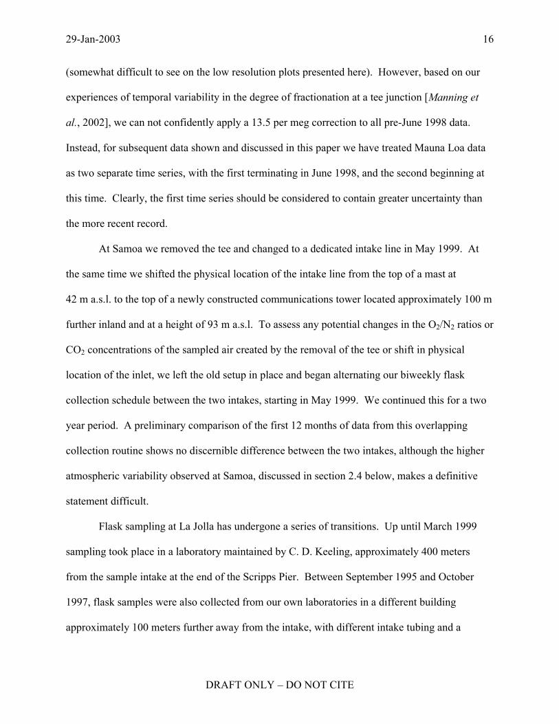
(somewhat difficult to see on the low resolution plots presented here). However, based on our

experiences of temporal variability in the degree of fractionation at a tee junction [Manning et

al., 2002], we can not confidently apply a 13.5 per meg correction to all pre-June 1998 data.

Instead, for subsequent data shown and discussed in this paper we have treated Mauna Loa data

as two separate time series, with the first terminating in June 1998, and the second beginning at

this time. Clearly, the first time series should be considered to contain greater uncertainty than

the more recent record.

At Samoa we removed the tee and changed to a dedicated intake line in May 1999. At

the same time we shifted the physical location of the intake line from the top of a mast at

42 m a.s.l. to the top of a newly constructed communications tower located approximately 100 m

further inland and at a height of 93 m a.s.l. To assess any potential changes in the O2/N2 ratios or

CO2 concentrations of the sampled air created by the removal of the tee or shift in physical

location of the inlet, we left the old setup in place and began alternating our biweekly flask

collection schedule between the two intakes, starting in May 1999. We continued this for a two

year period. A preliminary comparison of the first 12 months of data from this overlapping

collection routine shows no discernible difference between the two intakes, although the higher

atmospheric variability observed at Samoa, discussed in section 2.4 below, makes a definitive

statement difficult.

Flask sampling at La Jolla has undergone a series of transitions. Up until March 1999

sampling took place in a laboratory maintained by C. D. Keeling, approximately 400 meters

from the sample intake at the end of the Scripps Pier. Between September 1995 and October

1997, flask samples were also collected from our own laboratories in a different building

approximately 100 meters further away from the intake, with different intake tubing and a

29-Jan-2003

DRAFT ONLY – DO NOT CITE

17

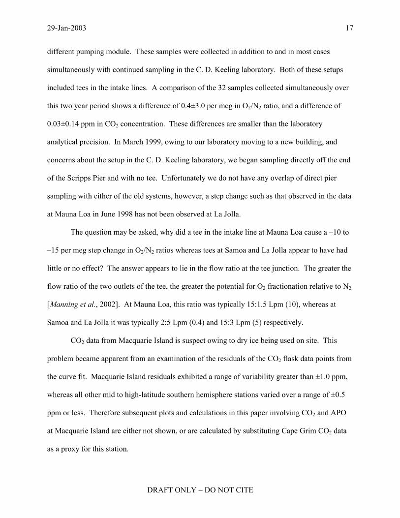
different pumping module. These samples were collected in addition to and in most cases

simultaneously with continued sampling in the C. D. Keeling laboratory. Both of these setups

included tees in the intake lines. A comparison of the 32 samples collected simultaneously over

this two year period shows a difference of 0.4±3.0 per meg in O2/N2 ratio, and a difference of

0.03±0.14 ppm in CO2 concentration. These differences are smaller than the laboratory

analytical precision. In March 1999, owing to our laboratory moving to a new building, and

concerns about the setup in the C. D. Keeling laboratory, we began sampling directly off the end

of the Scripps Pier and with no tee. Unfortunately we do not have any overlap of direct pier

sampling with either of the old systems, however, a step change such as that observed in the data

at Mauna Loa in June 1998 has not been observed at La Jolla.

The question may be asked, why did a tee in the intake line at Mauna Loa cause a –10 to

–15 per meg step change in O2/N2 ratios whereas tees at Samoa and La Jolla appear to have had

little or no effect? The answer appears to lie in the flow ratio at the tee junction. The greater the

flow ratio of the two outlets of the tee, the greater the potential for O2 fractionation relative to N2

[Manning et al., 2002]. At Mauna Loa, this ratio was typically 15:1.5 Lpm (10), whereas at

Samoa and La Jolla it was typically 2:5 Lpm (0.4) and 15:3 Lpm (5) respectively.

CO2 data from Macquarie Island is suspect owing to dry ice being used on site. This

problem became apparent from an examination of the residuals of the CO2 flask data points from

the curve fit. Macquarie Island residuals exhibited a range of variability greater than ±1.0 ppm,

whereas all other mid to high-latitude southern hemisphere stations varied over a range of ±0.5

ppm or less. Therefore subsequent plots and calculations in this paper involving CO2 and APO

at Macquarie Island are either not shown, or are calculated by substituting Cape Grim CO2 data

as a proxy for this station.

29-Jan-2003

DRAFT ONLY – DO NOT CITE

18

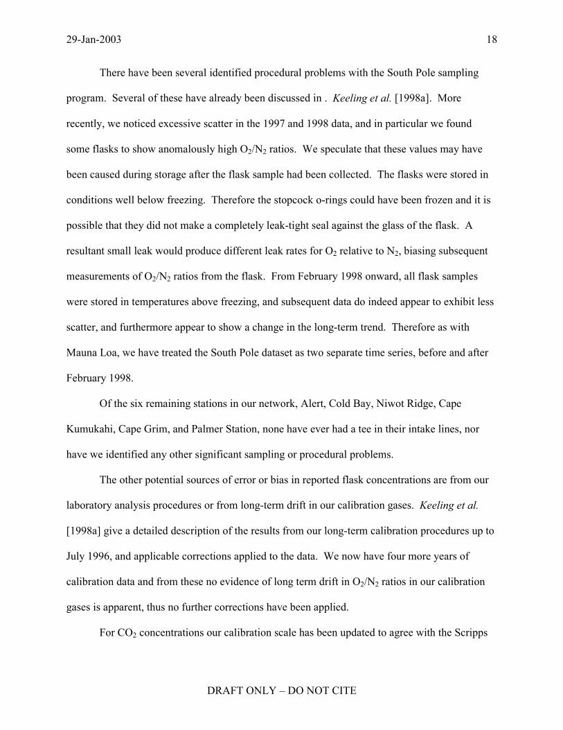
There have been several identified procedural problems with the South Pole sampling

program. Several of these have already been discussed in . Keeling et al. [1998a]. More

recently, we noticed excessive scatter in the 1997 and 1998 data, and in particular we found

some flasks to show anomalously high O2/N2 ratios. We speculate that these values may have

been caused during storage after the flask sample had been collected. The flasks were stored in

conditions well below freezing. Therefore the stopcock o-rings could have been frozen and it is

possible that they did not make a completely leak-tight seal against the glass of the flask. A

resultant small leak would produce different leak rates for O2 relative to N2, biasing subsequent

measurements of O2/N2 ratios from the flask. From February 1998 onward, all flask samples

were stored in temperatures above freezing, and subsequent data do indeed appear to exhibit less

scatter, and furthermore appear to show a change in the long-term trend. Therefore as with

Mauna Loa, we have treated the South Pole dataset as two separate time series, before and after

February 1998.

Of the six remaining stations in our network, Alert, Cold Bay, Niwot Ridge, Cape

Kumukahi, Cape Grim, and Palmer Station, none have ever had a tee in their intake lines, nor

have we identified any other significant sampling or procedural problems.

The other potential sources of error or bias in reported flask concentrations are from our

laboratory analysis procedures or from long-term drift in our calibration gases. Keeling et al.

[1998a] give a detailed description of the results from our long-term calibration procedures up to

July 1996, and applicable corrections applied to the data. We now have four more years of

calibration data and from these no evidence of long term drift in O2/N2 ratios in our calibration

gases is apparent, thus no further corrections have been applied.

For CO2 concentrations our calibration scale has been updated to agree with the Scripps

29-Jan-2003

DRAFT ONLY – DO NOT CITE

19

1999 manometric scale maintained by the C. D. Keeling laboratory, also at Scripps Institution of

Oceanography. We also noticed and corrected for a step change in the span of our CO2 analyser

in March 1993 which coincided with the change in physical location of our laboratory from

Boulder, Colorado, to La Jolla, California. This is perhaps not surprising since in Boulder the

CO2 analyser was actively controlled to ambient pressure which is approximately 830 mbar at

the altitude of Boulder. When we moved to La Jolla, situated at sea level, we changed the gas

handling design so as to continue to actively stabilize the CO2 analyser to 830 mbar. However, it

appears that despite our efforts, a change in the span of the analyser occurred. This change was

of the order of 0.4 ppm/Volt, which, for example, corresponded to a change in one reference gas

of about 0.1 ppm CO2. No changes in O2/N2 ratios in calibration gases relative to each other

were observed after the move to La Jolla.

During a two month period from September to November 1996 a diaphragm on a

compressor pump in the analysis system was leaking. This pump is located downstream of the

CO2 analyser and so did not affect CO2 concentrations, but, being upstream of the interferometric

O2 analyser, it resulted in a change in the O2/N2 ratio. Because our primary calibration gases

were analysed during this period, a correction could be applied to the 136 flasks that were

analysed and the data we show in Figures 2 and 4 have this correction applied.

3. Global Oceanic and Land Biotic Carbon Sinks

As mentioned in the Introduction, precise measurements of atmospheric O2, along with

concurrent CO2 measurements, allow estimates of global oceanic and land biotic carbon sinks to

be derived. In this section we present calculations of these sinks made over different time

periods and using data from different stations, and we compare our results with results from

29-Jan-2003

DRAFT ONLY – DO NOT CITE

20

other researchers.

The primary contribution to the interannual downward trend in O2/N2 ratios (and upward

trend in CO2 concentrations) is anthropogenic combustion of fossil fuels. Other processes can

also affect this trend such as biomass burning, anthropogenic land use changes, net uptake by the

land biota, and oceanic ventilation processes occurring on interannual time scales. Oceanic

uptake of atmospheric CO2, however, reduces the observed upward trend in atmospheric CO2

concentrations, but has no affect on the observed downward trend in O2/N2 ratios. Thus the

global budgets for atmospheric CO2 and O2 can be respectively represented by

∆CO2 = F – O – B, and

∆O2 = –αFF + αBB + Z,

where ∆CO2 is the globally averaged observed change in atmospheric CO2 concentration, ∆O2 is

the globally averaged observed change in atmospheric O2 concentration, F is the source of CO2

emitted from fossil fuel combustion (and cement manufacture), O is the oceanic CO2 sink, B is

the net land biotic CO2 sink (including biomass burning, land use changes, and land biotic

uptake), αF and αB are the global average O2:CO2 molar exchange ratios for fossil fuels and land

biota respectively, and Z is the net exchange of atmospheric O2 with the oceans. All quantities,

except for the exchange ratios, αF and αB, are expressed in units of moles per year.

In all calculations below, a value of 1.10±0.05 is used for αB [Severinghaus, 1995]. That

is, 1.1 moles of atmospheric O2 are produced for every mole of atmospheric CO2 consumed by

the land biota. An average value of 1.39±0.04 is used for αF which was calculated from a

knowledge of the amount of the different fossil fuel types combusted from year to year [Marland

et al., 2002], and from the average O2:C oxidative ratios for full combustion of each fuel type

[Keeling, 1988a]. This value for αF was found to change only negligibly for any of the different

(3)

(4)

29-Jan-2003

DRAFT ONLY – DO NOT CITE

21

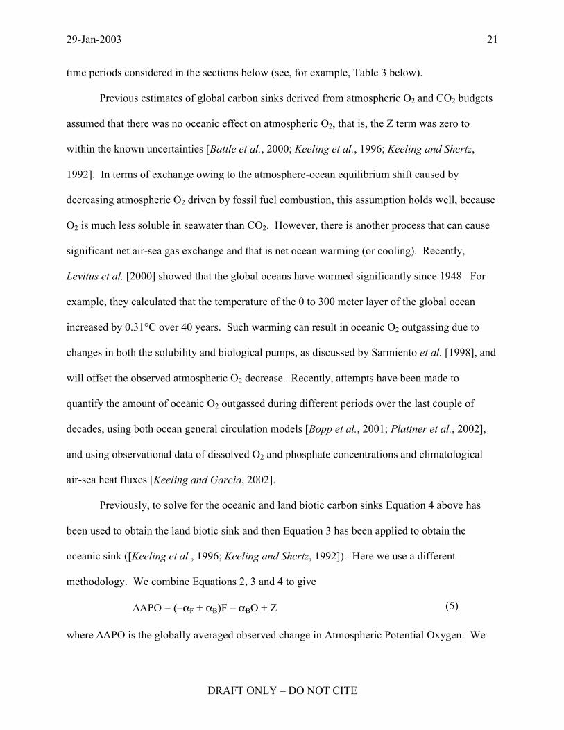
time periods considered in the sections below (see, for example, Table 3 below).

Previous estimates of global carbon sinks derived from atmospheric O2 and CO2 budgets

assumed that there was no oceanic effect on atmospheric O2, that is, the Z term was zero to

within the known uncertainties [Battle et al., 2000; Keeling et al., 1996; Keeling and Shertz,

1992]. In terms of exchange owing to the atmosphere-ocean equilibrium shift caused by

decreasing atmospheric O2 driven by fossil fuel combustion, this assumption holds well, because

O2 is much less soluble in seawater than CO2. However, there is another process that can cause

significant net air-sea gas exchange and that is net ocean warming (or cooling). Recently,

Levitus et al. [2000] showed that the global oceans have warmed significantly since 1948. For

example, they calculated that the temperature of the 0 to 300 meter layer of the global ocean

increased by 0.31°C over 40 years. Such warming can result in oceanic O2 outgassing due to

changes in both the solubility and biological pumps, as discussed by Sarmiento et al. [1998], and

will offset the observed atmospheric O2 decrease. Recently, attempts have been made to

quantify the amount of oceanic O2 outgassed during different periods over the last couple of

decades, using both ocean general circulation models [Bopp et al., 2001; Plattner et al., 2002],

and using observational data of dissolved O2 and phosphate concentrations and climatological

air-sea heat fluxes [Keeling and Garcia, 2002].

Previously, to solve for the oceanic and land biotic carbon sinks Equation 4 above has

been used to obtain the land biotic sink and then Equation 3 has been applied to obtain the

oceanic sink ([Keeling et al., 1996; Keeling and Shertz, 1992]). Here we use a different

methodology. We combine Equations 2, 3 and 4 to give

∆APO = (–αF + αB)F – αBO + Z

where ∆APO is the globally averaged observed change in Atmospheric Potential Oxygen. We

(5)

29-Jan-2003

DRAFT ONLY – DO NOT CITE

22

use Equation 5 to obtain the oceanic sink and then use Equation 3 to obtain the land biotic sink.

There are several reasons for using this methodology.

First, in deriving the oceanic sink, the uncertainty calculated from a quadrature sum of

errors is reduced by using Equation 5. Second, uncertainty is further reduced because short-term

(daily to seasonal) atmospheric variability is less in APO than in O2/N2 ratios. Third, we expect

longer term interannual variability in APO to be reduced compared to O2/N2 ratios because the

APO signal is not affected by interannual variability in the land biotic sink, and indeed APO data

shown in Figure 6 appear to confirm this, exhibiting less variability than comparative O2/N2 ratio

data in Figure 5 (These two figures are discussed in Section 4 below). Once we have obtained

the oceanic sink from Equation 5, we then have the choice of using either Equation 3 or 4 to

derive the land biotic sink. We chose to use Equation 3, both because it avoids applying the

oceanic O2 outgassing term a second time, a parameter which is known only very poorly, and

because with Equation 3 we have the option of using global atmospheric CO2 datasets from other

sources to derive ∆CO2, in particular the NOAA/CMDL global network, which has a much

denser global coverage than our own network, thus giving a more robust estimate of the land

biotic sink.

Several simplifying assumptions have been applied in formulating Equations 3, 4, and 5.

We assume that there is no longterm net change in marine productivity (which would affect

atmospheric O2); we assume no longterm (interannual) oceanic O2 ventilation other than that

associated with oceanic warming effects, accounted for in our Z term; we have included a Z

term for N2 as a correction factor to the observed atmospheric O2/N2 ratio, but we only calculate

oceanic N2 outgassing caused directly by changes in solubility resulting from ocean warming;

we assume that there is no Z term for CO2; and in Equation 5, we assume that the O2:CO2 molar

29-Jan-2003

DRAFT ONLY – DO NOT CITE

23

exchange ratio of all land biota (that is, αB) is 1.10, and that influences on APO due to oxidation

of CH4 and CO are negligible.

3.1. Calculation for the Decade of the 1990s

The data and results presented in this section have been used in the IPCC

(Intergovernmental Panel for Climate Change) Third Assessment Report ([Prentice et al.,

2001]), in their presentation of the oceanic and land biotic sinks for the decade of the 1990s. The

IPCC referenced Manning [2001]. However, Manning [2001] is a Ph.D. dissertation, and thus is

not a formally published or peer-reviewed document. For this reason, and because of the interest

shown by many workers, the work of Manning [2001] is duplicated here. Furthermore, we

provide detailed tables of data so that our calculations can be repeated by other researchers if

desired.

We calculate global averages of APO and CO2 by using data from selected stations in our

global network. For each station used we use the curve fits to the flask data shown in Figures 3

and 4 to adjust all flask data to the 15th of each month, then we calculate monthly means.

Months with no flask data are filled in using the curve fits. We average twelve consecutive

monthly means to compute annual means for APO and CO2, repeating this calculation at six-

month time steps centered on 1 January and 1 July of each year. The IPCC wished to report

global oceanic and land biotic carbon sinks for the entire decade of the 1990s so as to compare

these results with similar results computed for the 1980s decade. Eleven years of APO and CO2

data are needed in order to perform these calculations for the ten year period from 1 January

1990 to 1 January 2000. The technique subtracts an annual average centered on 1 January 2000

from an annual average centered on 1 January 1990, and therefore requires atmospheric

29-Jan-2003

DRAFT ONLY – DO NOT CITE

24

measurements spanning the period from 1 July 1989 to 1 July 2000. La Jolla is the only station

for which such a dataset exists. The Alert record comes close, with samples collected on two

dates in 1989, in November and December. Therefore our strategy is to use both the La Jolla and

Alert records, with a slightly different method of calculating the beginning point of the Alert

record.

In the Appendix we assess the robustness of the Alert beginning point calculation,

comment on not using any data from a southern hemisphere station, and detail other

considerations that were necessary to arrive at these particular results. Table 2 shows annual

averages of O2/N2 ratio data and calculated APO data for La Jolla, Alert, and the average of these

two stations. These APO annual averages are shown graphically as solid circles in Figure 7,

which shows also calculated annual averages of CO2. These data points show the expected

trends of decreasing APO over time and increasing CO2 concentrations.

We calculate the amount of CO2 produced from fossil fuel combustion and cement

manufacture from data in Marland et al. [2002]. We calculate the amount of O2 (and thus APO)

consumed from a knowledge of the relative fraction of the different fossil fuel types combusted

each year and the O2:CO2 oxidative ratios for each fuel type given in Keeling [1988a], assuming

full combustion of fossil fuel carbon to CO2. These data are shown in Table 3. For the ten year

period from January 1990 to January 2000 these fossil fuel emissions resulted in 63.3±3.8 Gt C

of CO2 being released to the atmosphere (F in Equations 3, 4, and 5; see also penultimate row of

Table 3), and, if no other processes were involved, would have resulted in a total APO decrease

of 41.8±2.5 per meg and an atmospheric CO2 increase of 29.8±1.8 ppm. These hypothetical

APO and CO2 changes are shown in Figure 7 as a straight line labelled “change due to fossil fuel

combustion only”. However, the observed atmospheric changes over this ten year period were

29-Jan-2003

DRAFT ONLY – DO NOT CITE

25

an APO decrease of 81.7±6.0 per meg (∆APO in Equation 5), and an atmospheric CO2 increase

of 15.11±0.61 ppm (32.1±1.3 Gt C; ∆CO2 in Equation 3). The value for ∆APO was found

simply by subtracting the 1990.0 mean from the 2000.0 mean (see Table 2). For ∆CO2,

however, as proposed above, we have used NOAA/CMDL data [Conway et al., 1994]. In this

particular calculation, this has the additional advantage of allowing us to include southern

hemisphere stations in the global average for ∆CO2 since the NOAA dataset includes such

stations extending back in time to at least 1990. Thus the global value for ∆CO2 was determined

(P. Tans, personal communication) using a 2-D atmospheric transport model described in Tans et

al. [Tans et al., 1989].

Setting the Z term (Equation 5) to zero for the moment, it is a useful exercise to calculate

average oceanic and land biotic sinks assuming no oceanic O2 outgassing term. From the data

above this results in:

oceanic carbon sink = 1.62±0.50 Gt C/y, and

land biotic carbon sink = 1.51±0.64 Gt C/y.

These results are illustrated graphically in Figure 7.

As mentioned above, the oceanic O2 outgassing term, Z, should incorporate effects due to

both the solubility and biological pumps. Three recent studies [Bopp et al., 2001; Keeling and

Garcia, 2002; Plattner et al., 2002] have produced estimates for Z, however, at the time the

IPCC report was published none of these studies had been completed. Therefore, in faithfulness

to our duplication of our work for the IPCC, we derive here our own estimate for the solubility-

only effect on oceanic O2 outgassing. Because the effects of ocean warming on the biological

pump are more complex and poorly understood, we make no attempt here to correct for any

possible effects.

29-Jan-2003

DRAFT ONLY – DO NOT CITE

26

We assume a 1 W/m2 warming rate over the global oceans during the 1990s (M.

Heimann, personal communication). This corresponds to a 0.71 W/m2 warming over the entire

surface of the Earth. Because of the uncertain nature of this calculation, we assign a 100%

uncertainty to this warming rate. 1 W/m2 results in a total of 1.14 x 1023 J of energy being

absorbed by the oceans during the decade of the 1990s. Using an O2 solubility temperature

dependence of 5.818 x 10-6 mol/kg/K [Weiss, 1970], this results in a total of 1.59 x 1014 mol O2

outgassed from the oceans in the 1990s. Net N2 outgassing from the oceans will also occur,

offsetting the increase in the atmospheric O2/N2 ratio. We calculate that 2.58 x 1014 mol N2

outgassed from the oceans in the 1990s, or 0.69 x 1014 mol O2 equivalent. Therefore 0.90 x 1014

mol O2 were effectively outgassed after applying this N2 correction. Recalculating the average

oceanic and land biotic carbon sinks in the 1990s results in:

oceanic carbon sink = 1.71±0.52 Gt C/y, and

land biotic carbon sink = 1.41±0.66 Gt C/y. 1

These results show that the global oceanic and land biotic carbon sinks are of

approximately comparable magnitude and importance in the global carbon budget. These results

also show an approximate 0.1 Gt C/y shift in both sinks when allowance is made for an ocean

warming effect with subsequent O2 outgassing caused by solubility pump changes, with the

oceanic sink becoming larger and the land biotic sink smaller. It is important to keep in mind

with these IPCC results that additional oceanic O2 outgassing most probably occurred owing to

1 There are two minor differences in the calculation presented here compared to that of Manning [, 2001 #725]. First, Manning [, 2001 #725] did not have available fossil fuel emission data from Marland et al. [, 2002 #653] through to the end of 1999, instead using data from British Petroleum for emissions in 1998 and 1999 (H. Kheshgi, personal communication). Second, at that time the Alert record went only as far as May 2000, two months short of the July 2000 required to achieve an annual average centred on 1 January 2000. Therefore a slightly different technique was used to obtain this year 2000 annual average. The resulting differences between the oceanic and land biotic sinks of Manning [, 2001 #725] and those presented here was only 0.03 Pg C/y. Therefore to a precision of one decimal place, as presented in the IPCC report, the results are the same.

29-Jan-2003

DRAFT ONLY – DO NOT CITE

27

biological pump changes induced by the ocean warming trend, and that this would result in a

larger oceanic carbon sink and a smaller land biotic carbon sink than calculated here.

We would also like to make it explicitly clear that this calculation technique effectively

determines a global oceanic carbon sink from northern hemisphere data only, then using this

oceanic sink result, the land biotic sink is calculated from globally averaged CO2 data. This

provides a more robust estimate of the land biotic sink, advantageous since the land sink exhibits

much greater natural variability than the oceanic sink (see section 3.4 below). In addition, the

land biotic sink can be expected to show greater north-south asymmetry than the oceanic sink,

thus greater bias would result if the land biotic sink was also calculated from northern

hemisphere-only data.

29-Jan-2003

DRAFT ONLY – DO NOT CITE

28

7. Appendix:

Additional Considerations for the 1990s Global Sinks Calculation

In this section we give further details on additional considerations that were necessary to

arrive at the global sink calculations presented in section 3.1. We also detail how we arrived at

the uncertainties given for these sinks. In the La Jolla dataset we discarded some data from flask

samples collected in 1990. This is pertinent to any comparison made to Keeling and Shertz

[1992], where our 1990 data were also used. In 1989 and 1990, some of the stopcocks on the

glass flasks sealed with Teflon o-rings, rather than Viton o-rings. Keeling and Shertz [1992],

observing very low O2 concentrations in some flask samples, realized that they were

contaminated, and attributed this problem to preferential diffusion of O2 relative to N2 through

the Teflon o-rings. Keeling and Shertz [1992] discarded many, but not all, of the samples

collected in these flasks. With the longer dataset now available, we were able to show that the

Teflon o-ring-sealed flasks retained by Keeling and Shertz [1992] also exhibited a small negative

O2 anomaly from the apparent baseline. Therefore we discarded all remaining samples collected

in Teflon o-ring-sealed flasks. Although CO2 concentrations were not affected by the Teflon o-

ring-sealed flasks, we removed CO2 data obtained from the same flasks also, so as not to cause

inconsistent aliasing of the two datasets. This removed seven sampling dates in 1990 from the

dataset, leaving a total of five dates when samples were collected from La Jolla in 1989 and three

in 1990 (in 1991 our regular sampling program was initiated and, for example, in this year 18

samples were collected). The raw data retained are shown in Figure 8a. Here we have shown

APO data only, and we have seasonally detrended the data, removing the four-harmonic

component of the curve fit from all data points. Therefore this figure shows the actual data used

to compute the annual means.

29-Jan-2003

DRAFT ONLY – DO NOT CITE

29

Because of the sparseness of the early part of the La Jolla record, we then proceeded to

look in more detail at the Alert record. If the Alert record shows a similar long-term trend as La

Jolla, then this will provide greater confidence in the La Jolla data. Flask samples were collected

on two dates at Alert in 1989, none in 1990, and 15 in 1991 when a regular sampling program

was begun. Figure 8b shows the Alert seasonally detrended APO.

In order to include the Alert data in the oceanic and land biotic sink calculations, annual

averages centered on 1 January 1990, and 1 January 2000 are needed, therefore requiring data

back to 1 July 1989, and up to 1 July 2000 in the normal calculation methods. Since in 1989 we

only have data from samples collected in November and December, our procedure to calculate

an “annual” average was as follows: The computer program used for calculating curve fits to the

data also reports monthly values of the curve fit on the 15th of each month, and reports

deseasonalized values for each month. Therefore we averaged four deseasonalized monthly

values, from November and December 1989, based on flask samples, and from January and

February 1990, based on interpolated monthly values of the curve fit, resulting in an average

centered on 1 January 1990.

The advantages of using APO data instead of O2/N2 ratio data have been mentioned in

Section 3 above. For the unique case of these IPCC calculations, using APO is even more

advantageous, helping reduce additional uncertainty that could have arisen both due to the

sparseness of the early La Jolla and Alert records, and the necessary interpolation of the early

Alert record. This becomes apparent when we compare longterm trends at La Jolla and Alert in

O2/N2 ratios and APO over different time periods. For the nine year period starting in 1991

when sampling programs were in full operation at both stations, the O2/N2 ratio trend differed by

about 5 per meg over the nine years. Whereas with the interpolated Alert dataset, and the sparse

29-Jan-2003

DRAFT ONLY – DO NOT CITE

30

early record of La Jolla added, the difference in the trends doubles to 10 per meg over ten years.

However, APO data over the same intervals (illustrated in Figure 8) show only a 2 per meg

difference in the Alert and La Jolla trends over nine years, and also a 2 per meg difference over

the longer ten year period. These findings provide confidence both in the use of APO data, and

in the Alert interpolation technique and subsequent averaging of Alert and La Jolla stations to

obtain a northern hemisphere proxy.

The final consideration in the IPCC calculation is the lack of southern hemisphere O2/N2

data in computing “global” carbon sinks. Not only is there an interhemispheric gradient in O2/N2

ratios and APO [Stephens et al., 1998], but these gradients exhibit significant interannual

variability. This makes it problematic to use only northern hemisphere stations in calculating a

global average. We attempted to quantify this additional error by comparing the Cape Grim

trend to the Alert and La Jolla trends over the time period for which we have Cape Grim data,

which is a 9.5 year measurement period from January 1991 to July 2000. Over this time period,

the O2/N2 ratio at Cape Grim decreased by about 15 per meg more than at the two northern

hemisphere stations. In APO the difference was less, but still high at about 10 per meg. Since in

a true global calculation the southern hemisphere would contribute a weighting of one-half to the

global trend, we decided to add ±3 per meg uncertainty to the reported APO trend because of this

lack of southern hemisphere data.

A summary of the uncertainties assigned to the different variables used in the global sinks

calculation is shown in Table 4. The total uncertainty in the assigned global APO trend is ±8.2

per meg. This was derived from a quadrature sum of the ±6 per meg uncertainty for a typical

global O2/N2 (or APO) trend computation [Keeling et al., 1996], ±3 per meg attributed to the

lack of southern hemisphere data, ±3.4 per meg additional uncertainty attributed to sparse data in

29-Jan-2003

DRAFT ONLY – DO NOT CITE

31

the early Alert record and the Alert interpolation, and ±3.2 per meg attributed to the sparse La

Jolla data in 1989 and 1990. These latter two uncertainties were calculated by considering the

residuals of the flask data from the curve fits of the full Alert and La Jolla records. These

residuals are shown in Figure 9. The standard deviation of these residuals was calculated for the

full record, then the standard error was calculated by considering how many flask samples were

used in deriving the 1990 annual averages. Figure 9 also aids in verifying that the 1989 and

1990 data are not unusual in terms of their residuals from the fitted curves.

8. References

Bacastow, R.B., C.D. Keeling, T.J. Lueker, M. Wahlen, and W.G. Mook, The 13C Suess effect in the world surface oceans and its implications for oceanic uptake of CO2: Analysis of observations at Bermuda, Global Biogeochemical Cycles, 10 (2), 335-346, 1996.

Balkanski, Y., P. Monfray, M. Battle, and M. Heimann, Ocean primary production derived from satellite data: An evaluation with atmospheric oxygen measurements, Global Biogeochemical Cycles, 13 (2), 257-271, 1999.

Battle, M., M. Bender, T. Sowers, P.P. Tans, J.H. Butler, J.W. Elkins, J.T. Ellis, T. Conway, N. Zhang, P. Lang, and A.D. Clarke, Atmospheric gas concentrations over the past century measured in air from firn at the South Pole, Nature, 383, 231-235, 1996.

Battle, M., M.L. Bender, P.P. Tans, J.W.C. White, J.T. Ellis, T. Conway, and R.J. Francey, Global carbon sinks and their variability inferred from atmospheric O2 and δ13C, Science, 287 (5462), 2467-2470, 2000.

Bender, M., T. Ellis, P. Tans, R. Francey, and D. Lowe, Variability in the O2/N2 ratio of southern hemisphere air, 1991-1994: Implications for the carbon cycle, Global Biogeochemical Cycles, 10 (1), 9-21, 1996.

Bender, M.L., M. Battle, and R.F. Keeling, The O2 balance of the atmosphere: A tool for studying the fate of fossil-fuel CO2, Annu. Rev. Energy Environ., 23, 207-223, 1998.

Bender, M.L., and M.O. Battle, Carbon cycle studies based on the distribution of O2 in air, Tellus Series B-Chemical and Physical Meteorology, 51 (2), 165-169, 1999.

Bender, M.L., T. Sowers, J.M. Barnola, and J. Chappellaz, Changes in the O2/N2 ratio of the atmosphere during recent decades reflected in the composition of air in the firn at Vostok Station, Antarctica, Geophysical Research Letters, 21, 189-192, 1994a.

Bender, M.L., P.P. Tans, J.T. Ellis, J. Orchardo, and K. Habfast, A high precision isotope ratio mass spectrometry method for measuring the O2/N2 ratio of air, Geochimica et Cosmochimica Acta, 58 (21), 4751-4758, 1994b.

Benedict, F.G., The Composition of the Atmosphere with Special Reference to its Oxygen Content, Carnegie Institution of Washington, 1912.

Bloom, A.J., R.M. Caldwell, J. Finazzo, R.L. Warner, and J. Weissbart, Oxygen and carbon

29-Jan-2003

DRAFT ONLY – DO NOT CITE

32

dioxide fluxes from barley shoots depend on nitrate assimilation, Plant Physiology, 91 (1), 352-356, 1989.

Bopp, L., C. Le Quere, M. Heimann, A.C. Manning, and P. Monfray, Climate-induced oceanic oxygen fluxes: Implications for the contemporary carbon budget, GBC, 2001.

Carpenter, T.M., The constancy of the atmosphere with respect to carbon dioxide and oxygen content, J. Amer. Chem. Soc., 59, 358-360, 1937.

Ciais, P., P.P. Tans, J.W.C. White, M. Trolier, R.J. Francey, J.A. Berry, D.R. Randall, P.J. Sellers, J.G. Collatz, and D.S. Schimel, Partitioning of ocean and land uptake of CO2 as inferred by δ13C measurements from the NOAA Climate Monitoring and Diagnostics Laboratory Global Air Sampling Network, Journal of Geophysical Research, 100 (D3), 5051-5070, 1995.

Conway, T.J., P.P. Tans, L.S. Waterman, K.W. Thoning, D.R. Kitzis, K.A. Masarie, and N. Zhang, Evidence for interannual variability of the carbon cycle from the NOAA/CMDL global air sampling network, Journal of Geophysical Research, 99 (D11), 22,831-22,855, 1994.

Enting, I.G., C.M. Trudinger, and R.J. Francey, A synthesis inversion of the concentration and δ13C of atmospheric CO2, Tellus Series B-Chemical and Physical Meteorology, 47 (1-2), 35-52, 1995.

GLOBALVIEW-CO2, GLOBALVIEW-CO2: Cooperative Atmospheric Data Integration Project - Carbon Dioxide, CD-ROM, NOAA/CMDL, Boulder, Colorado. [Also available on Internet via anonymous FTP to ftp.cmdl.noaa.gov, Path: ccg/co2/GLOBALVIEW], 1999.

Graedel, T.E., and P.J. Crutzen, Atmospheric change: an Earth system perspective, 446 pp., W. H. Freeman and Company, New York, 1993.

Gruber, N., and C.D. Keeling, The isotopic air-sea disequilibrium and the oceanic uptake of anthropogenic CO2, in Proceedings of the 2nd International Symposium, CO2 in the Oceans, Center for Global Environmental Research, National Institute for Environmental Studies, Tsukuba, Japan, 1999.

Heimann, M., C.D. Keeling, and C.J. Tucker, A three-dimensional model of atmospheric CO2 transport based on observed winds: 3. Seasonal cycle and synoptic time scale variations, in Geophysical Monograph 55, Aspects of climate variability in the Pacific and the Western Americas, edited by D.H. Peterson, pp. 277-303, American Geophysical Union, Washington D. C., 1989.

Heimann, M., and E. Maier-Reimer, On the relations between the oceanic uptake of CO2 and its carbon isotopes, Global Biogeochemical Cycles, 10 (1), 89-110, 1996.

Keeling, C.D., S.C. Piper, and M. Heimann, A three-dimensional model of atmospheric CO2 transport based on observed winds: 4. Mean annual gradients and interannual variations, in Geophysical Monograph 55, Aspects of climate variability in the Pacific and the Western Americas, edited by D.H. Peterson, pp. 305-363, American Geophysical Union, Washington D. C., 1989.

Keeling, R.F., Development of an interferometric oxygen analyzer for precise measurement of the atmospheric O2 mole fraction, Ph.D. thesis, Harvard University, Cambridge, Massachusetts, U.S.A., 1988a.

Keeling, R.F., Measuring correlations between atmospheric oxygen and carbon dioxide mole fractions: A preliminary study in urban air, Journal of Atmospheric Chemistry, 7, 153-176, 1988b.

29-Jan-2003

DRAFT ONLY – DO NOT CITE

33

Keeling, R.F., and H.E. Garcia, The change in oceanic O2 inventory associated with recent global warming, Proceedings of the National Academy of Sciences of the United States of America, 99 (12), 7848-7853, 2002.

Keeling, R.F., A.C. Manning, E.M. McEvoy, and S.R. Shertz, Methods for measuring changes in atmospheric O2 concentration and their applications in southern hemisphere air, Journal of Geophysical Research, 103 (D3), 3381-3397, 1998a.

Keeling, R.F., R.P. Najjar, M.L. Bender, and P.P. Tans, What atmospheric oxygen measurements can tell us about the global carbon cycle, Global Biogeochemical Cycles, 7 (1), 37-67, 1993.

Keeling, R.F., S.C. Piper, and M. Heimann, Global and hemispheric CO2 sinks deduced from changes in atmospheric O2 concentration, Nature, 381, 218-221, 1996.

Keeling, R.F., and S.R. Shertz, Seasonal and interannual variations in atmospheric oxygen and implications for the global carbon cycle, Nature, 358, 723-727, 1992.

Keeling, R.F., B.B. Stephens, R.G. Najjar, S.C. Doney, D. Archer, and M. Heimann, Seasonal variations in the atmospheric O2/N2 ratio in relation to the kinetics of air-sea gas exchange, Global Biogeochemical Cycles, 12 (1), 141-163, 1998b.

Langenfelds, R.L., R.J. Francey, L.P. Steele, M. Battle, R.F. Keeling, and W.F. Budd, Partitioning of the global fossil CO2 sink using a 19-year trend in atmospheric O2, Geophysical Research Letters, 26 (13), 1897-1900, 1999.

Levitus, S., J.I. Antonov, T.P. Boyer, and C. Stephens, Warming of the world ocean, Science, 287 (5461), 2225-2229, 2000.

Liss, P.S., and L. Merlivat, Air-sea gas exchange rates: Introduction and synthesis, in The Role of Air-Sea Exchange in Geochemical Cycling, edited by P. Buat-Menard, pp. 113-127, D Reidel, Norwell, Mass, 1986.

Machta, L., Oxygen depletion, in Proceedings of the International Meeting on Stable Isotopes in Tree Ring Research, edited by G.C. Jacoby, pp. 125-127, 1980.

Machta, L., and E. Hughes, Atmospheric oxygen in 1967 to 1970, Science, 168, 1582-1584, 1970.

Mann, M.E., R.S. Bradley, and M.K. Hughes, Global-scale temperature patterns and climate forcing over the past six centuries, Nature, 392 (6678), 779-787, 1998.

Manning, A.C., Temporal variability of atmospheric oxygen from both continuous measurements and a flask sampling network: Tools for studying the global carbon cycle, Ph. D. thesis, University of California, San Diego, La Jolla, California, U.S.A., 2001.

Manning, A.C., and R.F. Keeling, Correlations in short-term variations in atmospheric oxygen and carbon dioxide at Mauna Loa Observatory, in Climate Monitoring and Diagnostics Laboratory, No. 22, Summary Report 1993, edited by J.T. Peterson, and R.M. Rosson, pp. 121-123, U.S. Department of Commerce, NOAA Environmental Research Laboratories, Boulder, CO, 1994.

Manning, A.C., R.F. Keeling, and J.P. Severinghaus, Precise atmospheric oxygen measurements with a paramagnetic oxygen analyzer, Global Biogeochemical Cycles, 13 (4), 1107-1115, 1999.

Manning, A.C., M.R. Manning, G.W. Brailsford, A.J. Gomez, R.F. Keeling, W.J. Paplawsky, and C.G. Atwood, Oceanic and terrestrial contributions to atmospheric O2 and CO2 derived from continuous measurements at Baring Head, New Zealand, 2002.

Marland, G., T.A. Boden, and R.J. Andres, Global, Regional, and National Annual CO2 Emissions from Fossil-Fuel Burning, Cement Production, and Gas Flaring: 1751-1999,

29-Jan-2003

DRAFT ONLY – DO NOT CITE

34

Carbon Dioxide Information Analysis Center, Oak Ridge National Laboratory, U.S. Department of Energy, Oak Ridge, Tenn., U.S.A., 2002.

Orr, J.C., Ocean Carbon-Cycle Model Intercomparison Project (OCMIP), 27 pp., 1997. Peixoto, J.P., and A.H. Oort, Physics of climate, 520 pp., American Institute of Physics, New

York, 1992. Plattner, G.K., F. Joos, and T.F. Stocker, Revision of the global carbon budget due to changing

air-sea oxygen fluxes, GBC, 2002. Prentice, I.C., G.D. Farquhar, M.J.R. Fasham, M.L. Goulden, M. Heimann, V.J. Jaramillo, H.S.

Kheshgi, C. Le Quéré, R.J. Scholes, and D.W.R. Wallace, The Carbon Cycle and Atmospheric CO2, in Climate Change 2001: The Scientific Basis.

Contribution of Working Group I to the Third Assessment Report of the Intergovernmental Panel on Climate Change (IPCC), edited by J.T. Houghton, Y. Ding, D.J. Griggs, M. Noguer, P.J. van der Linden, and D. Xiaosu, pp. 944, Cambridge University Press, Cambridge, 2001.

Quay, P.D., B. Tilbrook, and C.S. Wong, Oceanic uptake of fossil fuel CO2: Carbon-13 evidence, Science, 256, 74-79, 1992.

Reinsch, C.M., Smoothing by spline functions, Num. Math., 10, 177-183, 1967. Sarmiento, J.L., T.M.C. Hughes, R.J. Stouffer, and S. Manabe, Simulated response of the ocean

carbon cycle to anthropogenic climate warming, Nature, 393, 245-249, 1998. Severinghaus, J.P., Studies of the terrestrial O2 and carbon cycles in sand dune gases and in

Biosphere 2, Ph.D. thesis, Columbia University, New York, U.S.A., 1995. Stephens, B.B., Field-based atmospheric oxygen measurements and the ocean carbon cycle, Ph.

D. thesis, University of California, San Diego, La Jolla, California, U.S.A., 1999. Stephens, B.B., R.F. Keeling, M. Heimann, K.D. Six, R. Murnane, and K. Caldeira, Testing

global ocean carbon cycle models using measurements of atmospheric O2 and CO2 concentration, in Global Biogeochemical Cycles, 1997.

Stephens, B.B., R.F. Keeling, M. Heimann, K.D. Six, R. Murnane, and K. Caldeira, Testing global ocean carbon cycle models using measurements of atmospheric O2 and CO2 concentration, Global Biogeochemical Cycles, 12 (2), 213-230, 1998.

Takahashi, T., R.H. Wanninkhof, R.A. Feely, R.F. Weiss, D.W. Chipman, N. Bates, J. Olafsson, C. Sabine, and S.C. Sutherland, Net sea-air CO2 flux over the global oceans: an improved estimate based on the sea-air CO2 difference, in Proceedings of the 2nd International Symposium, CO2 in the Oceans, pp. 9-14, Center for Global Environmental Research, National Institute for Environmental Studies, Tsukuba, Japan, 1999.

Tans, P.P., P.S. Bakwin, and D.W. Guenther, A feasible global carbon cycle observing system: A plan to decipher today's carbon cycle based on observations, Global Change Biology, 2, 309-318, 1996.

Tans, P.P., J.A. Berry, and R.F. Keeling, Oceanic 13C/12C observations: a new window on ocean CO2 uptake, Global Biogeochemical Cycles, 7 (2), 353-368, 1993.

Tans, P.P., T.J. Conway, and T. Nakazawa, Latitudinal distribution of the sources and sinks of atmospheric carbon dioxide derived from surface observations and an atmospheric transport model, Journal of Geophysical Research, 94 (D4), 5151-5172, 1989.

Tans, P.P., I.Y. Fung, and T. Takahashi, Observational constraints on the global atmospheric CO2 budget, Science, 247, 1431-1438, 1990.

Tohjima, Y., Method for measuring changes in the atmospheric O2/N2 ratio by a gas chromatograph equipped with a thermal conductivity detector, Journal of Geophysical

29-Jan-2003

DRAFT ONLY – DO NOT CITE

35

Research-Atmospheres, 105 (D11), 14575-14584, 2000. Weiss, R.F., The solubility of nitrogen, oxygen and argon in water and seawater, Deep-Sea

Research, 17, 721-735, 1970.

-

Table 1. Flask Sampling Stations in the Scripps O2/N2 Network Station code

Station Latitude Longitude Elevation (m a.s.l.)

Time period

ALT Alert, Northwest Territories, Canada 82°27’N 62°31’W 210 Nov. 1989 – May 2000 CBA Cold Bay, Alaska, USA 55°12’N 162°43’W 25 Aug. 1995 – May 2000 NWR Niwot Ridge, Colorado, USA 40°03’N 105°38’W 3749 Apr. 1991 – Apr. 1993 LJO La Jolla, California, USA 32°52’N 117°15’W 15 May 1989 – June 2000 MLO Mauna Loa, Hawaii, USA 19°32’N 155°35’W 3397 Jan. 1991 – May 2000 KUM Cape Kumukahi, Hawaii, USA 19°31’N 154°49’W 3 June 1993 – May 2000 SMO Cape Matatula, American Samoa, USA 14°15’S 170°34’W 42/93* June 1993 – Apr. 2000 CGO Cape Grim, Tasmania, Australia 40°41’S 144°41’E 94 Jan. 1991 – Dec. 1999 MCQ Macquarie Island, Australia 54°29’S 158°58’E 94 Sep. 1992 – Jan. 1994 PSA Palmer Station, Antarctica 64°55’S 64°00’W 10 Sep. 1996 – Mar. 2000 SPO South Pole Station, Antarctica 89°59’S 24°48’W 2810 Nov. 1991 – Dec 1999 * In May 1999 a new sampling intake was installed on a new tower, 93 m above sea level.

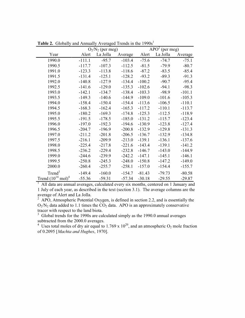
Table 2. Globally and Annually Averaged Trends in the 1990s1 O2/N2 (per meg) APO2 (per meg)

Year Alert La Jolla Average Alert La Jolla Average 1990.0 -111.1 -95.7 -103.4 -75.6 -74.7 -75.1 1990.5 -117.7 -107.3 -112.5 -81.5 -79.9 -80.7 1991.0 -123.3 -113.8 -118.6 -87.2 -83.5 -85.4 1991.5 -131.4 -125.1 -128.2 -93.2 -89.3 -91.3 1992.0 -140.8 -127.9 -134.4 -100.2 -90.7 -95.4 1992.5 -141.6 -129.0 -135.3 -102.6 -94.1 -98.3 1993.0 -142.1 -134.7 -138.4 -103.3 -98.9 -101.1 1993.5 -149.3 -140.6 -144.9 -109.0 -101.6 -105.3 1994.0 -158.4 -150.4 -154.4 -113.6 -106.5 -110.1 1994.5 -168.3 -162.4 -165.3 -117.2 -110.1 -113.7 1995.0 -180.2 -169.3 -174.8 -125.3 -112.5 -118.9 1995.5 -191.5 -178.5 -185.0 -131.2 -115.7 -123.4 1996.0 -197.0 -192.3 -194.6 -130.9 -123.8 -127.4 1996.5 -204.7 -196.9 -200.8 -132.9 -129.8 -131.3 1997.0 -211.2 -201.8 -206.5 -136.7 -132.9 -134.8 1997.5 -216.1 -209.9 -213.0 -139.1 -136.1 -137.6 1998.0 -225.4 -217.8 -221.6 -143.4 -139.1 -141.2 1998.5 -236.2 -229.4 -232.8 -146.7 -143.0 -144.9 1999.0 -244.6 -239.9 -242.2 -147.1 -145.1 -146.1 1999.5 -250.8 -245.3 -248.0 -150.8 -147.2 -149.0 2000.0 -260.4 -255.7 -258.1 -157.0 -154.4 -155.7 Trend3 -149.4 -160.0 -154.7 -81.43 -79.73 -80.58

Trend (1014 mol)4 -55.36 -59.31 -57.34 -30.18 -29.55 -29.87 1 All data are annual averages, calculated every six months, centered on 1 January and 1 July of each year, as described in the text (section 3.1). The average columns are the average of Alert and La Jolla. 2 APO, Atmospheric Potential Oxygen, is defined in section 2.2, and is essentially the O2/N2 data added to 1.1 times the CO2 data. APO is an approximately conservative tracer with respect to the land biota. 3 Global trends for the 1990s are calculated simply as the 1990.0 annual averages subtracted from the 2000.0 averages. 4 Uses total moles of dry air equal to 1.769 x 1020, and an atmospheric O2 mole fraction of 0.2095 [Machta and Hughes, 1970].

Table 3. Global Fossil Fuel Combustion Data for the 1990s

Year

CO2 produced1

(106 tonnes)2

O2 consumed3 (106 tonnes)

O2:C molar ratio

1990 6,104 22,581 1.3891991 6,183 22,955 1.394 1992 6,095 22,546 1.388 1993 6,073 22,514 1.391 1994 6,221 23,029 1.389 1995 6,407 23,752 1.392 1996 6,517 24,181 1.393 1997 6,601 24,517 1.394 1998 6,566 24,339 1999 6,521 24,172 Total 63,288 234,587 1.3914

Total (1014 mol) 52.70 73.32 1 Data are from Marland et al. [2000], and include CO2 produced from solid, liquid, and gas fuel, as well as from flared gas and cement manufacture. 2 106 tonnes is equivalent to 0.001 Gt, or 0.001 Pg. 3 O2 consumed is calculated assuming full combustion of all fossil fuel types, and using O2:CO2 molar ratios for each fuel type from Keeling [1988a]. That is, O2:CO2 is 1.17 for solid fuel; 1.44 for liquid fuel; 1.95 for gas fuel; and 1.98 for flared gas. (Cement manufacture does not consume O2.) 4 Average O2:CO2 molar ratio.

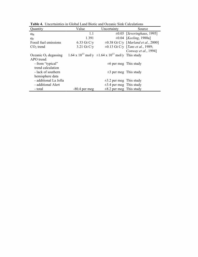
Table 4. Uncertainties in Global Land Biotic and Oceanic Sink Calculations Quantity Value Uncertainty Source αB 1.1 ±0.05 [Severinghaus, 1995] αF 1.391 ±0.04 [Keeling, 1988a] Fossil fuel emissions 6.33 Gt C/y ±0.38 Gt C/y [Marland et al., 2000] CO2 trend 3.21 Gt C/y ±0.13 Gt C/y [Tans et al., 1989;

Conway et al., 1994] Oceanic O2 degassing 1.64 x 1013 mol/y ±1.64 x 1013 mol/y This study APO trend:

- from “typical” trend calculation

±6 per meg This study

- lack of southern hemisphere data

±3 per meg This study

- additional La Jolla ±3.2 per meg This study - additional Alert ±3.4 per meg This study - total -80.4 per meg ±8.2 per meg This study

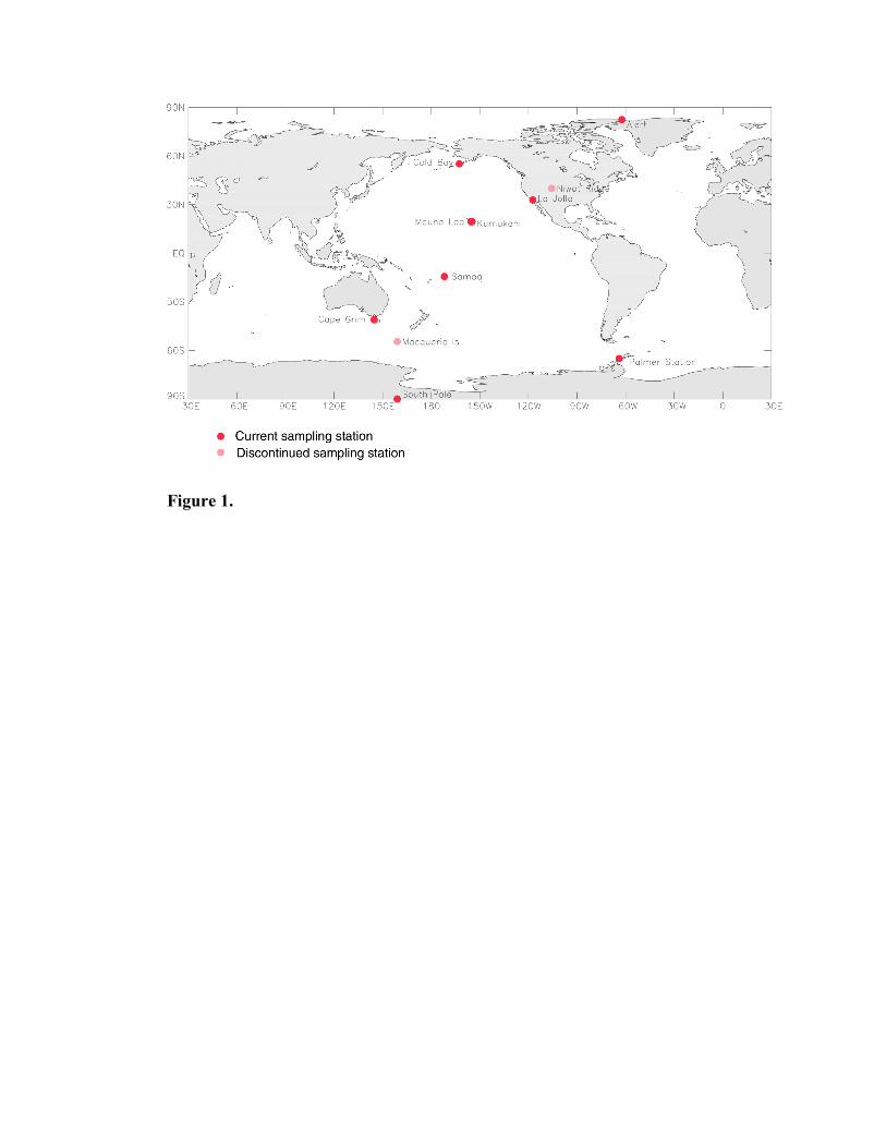
Figure 1.

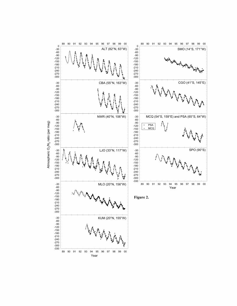
MCQ (54°S, 159°E) and PSA (65°S, 64°W)

Year

-300-270-240-210-180-150-120

-90-60-30

ALT (82°N, 63°W)

89 90 91 92 93 94 95 96 97 98 99 00

-300-270-240-210-180-150-120

-90-60-30

0

CBA (55°N, 163°W)

-300-270-240-210-180-150-120

-90-60-30

LJO (33°N, 117°W)

-300-270-240-210-180-150-120

-90-60-30

MLO (20°N, 156°W)

Year

Atm

osph

eric

O2/N

2 rat

io (p

er m

eg)

-300-270-240-210-180-150-120

-90-60-30

KUM (20°N, 155°W)

89 90 91 92 93 94 95 96 97 98 99 00-330-300-270-240-210-180-150-120

-90-60-30

SMO (14°S, 171°W)

89 90 91 92 93 94 95 96 97 98 99 00

-300-270-240-210-180-150-120

-90-60-30

0

CGO (41°S, 145°E)

-300-270-240-210-180-150-120

-90-60-30

SPO (90°S)

Year89 90 91 92 93 94 95 96 97 98 99 00

-330-300-270-240-210-180-150-120

-90-60-30

NWR (40°N, 106°W)

-300-270-240-210-180-150-120

-90-60-30

PSAMCQ

Figure 2.

MCQ (54°S, 159°E) and PSA (65°S, 64°W)

Year

348351354357360363366369372375

ALT (82°N, 63°W)

89 90 91 92 93 94 95 96 97 98 99 00

348351354357360363366369372375378

CBA (55°N, 163°W)

348351354357360363366369372375

LJO (33°N, 117°W)

348351354357360363366369372375

MLO (20°N, 156°W)

Year

Atm

osph

eric

CO

2 con

cent

ratio

n (p

pm)

348351354357360363366369372375

KUM (20°N, 155°W)

89 90 91 92 93 94 95 96 97 98 99 00345348351354357360363366369372375

SMO (14°S, 171°W)

89 90 91 92 93 94 95 96 97 98 99 00

348351354357360363366369372375378

CGO (41°S, 145°E)

348351354357360363366369372375

SPO (90°S)

Year89 90 91 92 93 94 95 96 97 98 99 00

345348351354357360363366369372375

NWR (40°N, 106°W)

348351354357360363366369372375

PSAMCQ

Figure 3.

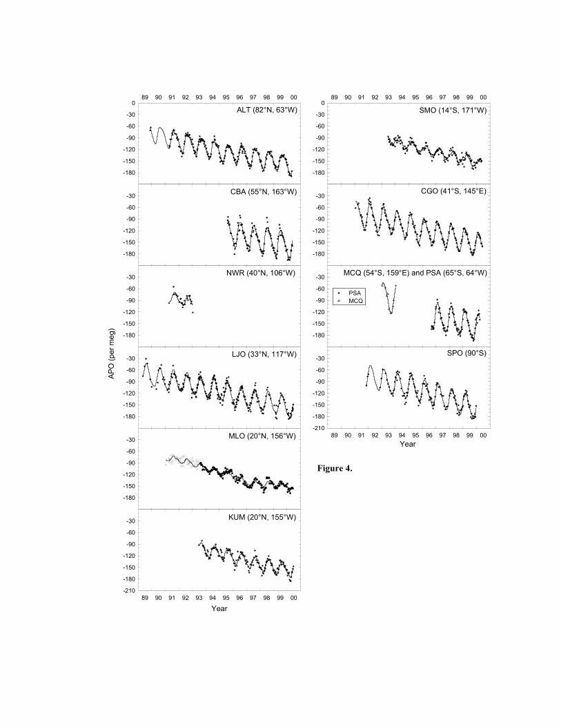
MCQ (54°S, 159°E) and PSA (65°S, 64°W)

Year

-180

-150

-120

-90

-60

-30

ALT (82°N, 63°W)

89 90 91 92 93 94 95 96 97 98 99 00

-180

-150

-120

-90

-60

-30

0

CBA (55°N, 163°W)

-180

-150

-120

-90

-60

-30

LJO (33°N, 117°W)

-180

-150

-120

-90

-60

-30

MLO (20°N, 156°W)

Year

APO

(per

meg

)

-180

-150

-120

-90

-60

-30

KUM (20°N, 155°W)

89 90 91 92 93 94 95 96 97 98 99 00-210

-180

-150

-120

-90

-60

-30

SMO (14°S, 171°W)

89 90 91 92 93 94 95 96 97 98 99 00

-180

-150

-120

-90

-60

-30

0

CGO (41°S, 145°E)

-180

-150

-120

-90

-60

-30

SPO (90°S)

Year89 90 91 92 93 94 95 96 97 98 99 00

-210

-180

-150

-120

-90

-60

-30

NWR (40°N, 106°W)

-180

-150

-120

-90

-60

-30

PSAMCQ

Figure 4.

PSA (65°S, 64°W)-60

-40

-20

0

20

ALT (82°N, 63°W)

91 92 93 94 95 96 97 98 99 00

-60

-40

-20

0

20

CBA (55°N, 163°W)

-60

-40

-20

0

20

LJO (33°N, 117°W)

-60

-40

-20

0

20

MLO (20°N, 156°W)

Des

easo

naliz

ed m

onth

y O

2/N2 r

atio

ave

rage

s di

ffere

nced

from

CG

O s

plin

e (p

er m

eg)

-60

-40

-20

0

20

KUM (20°N, 155°W)

91 92 93 94 95 96 97 98 99 00

-60

-40

-20

0

20

SMO (14°S, 171°W)

91 92 93 94 95 96 97 98 99 00

-60

-40

-20

0

20

SPO (90°S)

Year91 92 93 94 95 96 97 98 99 00

-60

-40

-20

0

20

CGO (41°S, 145°E)

91 92 93 94 95 96 97 98 99 00

Des

easo

naliz

ed

O2/N

2 rat

io a

t CG

O (p

er m

eg)

-300-270-240-210-180-150-120-90-60

Year

Figure 5.

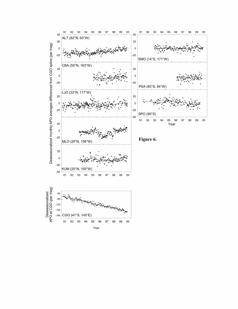
PSA (65°S, 64°W)-20

0

20

ALT (82°N, 63°W)

91 92 93 94 95 96 97 98 99 00

-20

0

20

40

CBA (55°N, 163°W)

-20

0

20

LJO (33°N, 117°W)

-20

0

20

MLO (20°N, 156°W)

Dea

seas

onal

ized

mon

thly

APO

ave

rage

s di

ffere

nced

from

CG

O s

plin

e (p

er m

eg)

-20

0

20

KUM (20°N, 155°W)

91 92 93 94 95 96 97 98 99 00-40

-20

0

20

SMO (14°S, 171°W)

91 92 93 94 95 96 97 98 99 00

-20

0

20

40

SPO (90°S)

Year91 92 93 94 95 96 97 98 99 00

-40

-20

0

20

CGO (41°S, 145°E)

Year

91 92 93 94 95 96 97 98 99 00

Dea

seas

onal

ized

APO

at C

GO

(per

meg

)

-180

-150

-120

-90

-60

Figure 6.

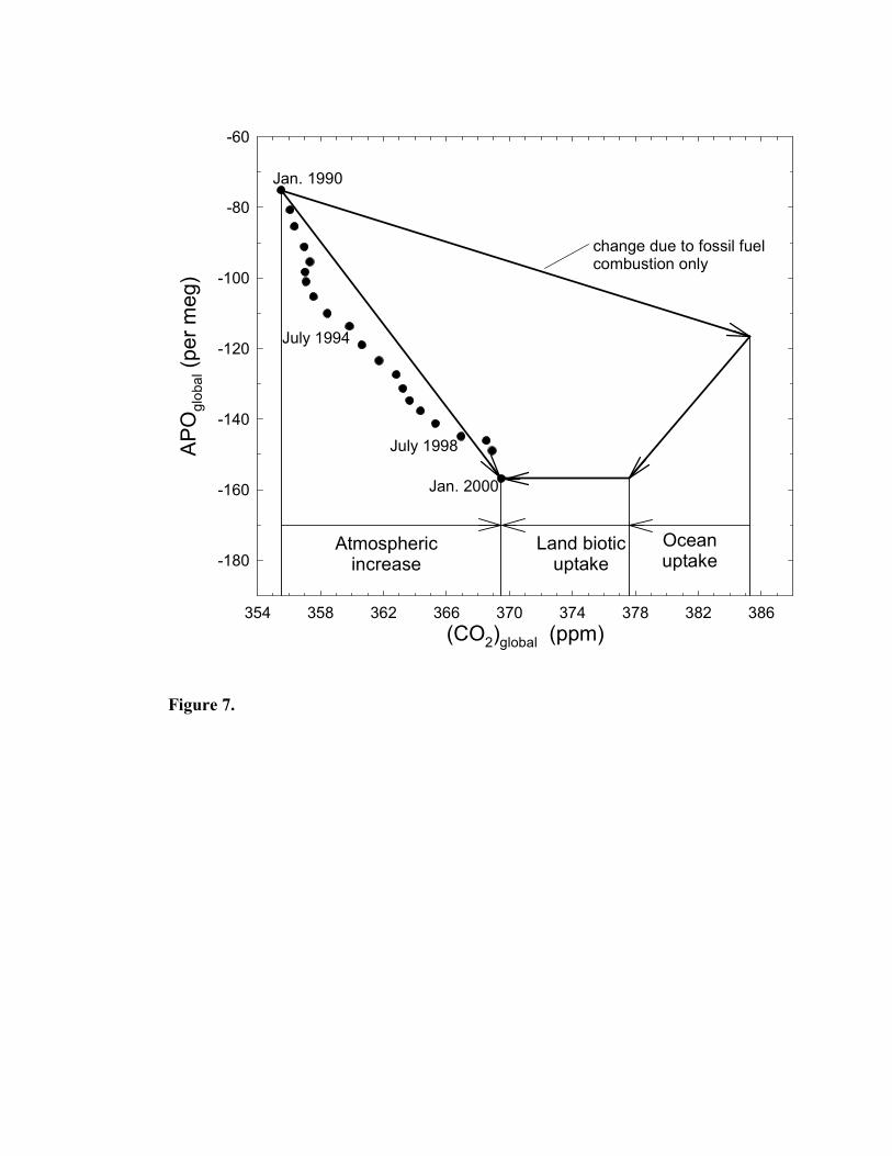
Figure 7.

Oceanuptake

(CO2)global (ppm)354 358 362 366 370 374 378 382 386

APO

glob

al (p

er m

eg)

-180

-160

-140

-120

-100

-80

-60

Jan. 1990

July 1998

July 1994

change due to fossil fuelcombustion only

Atmosphericincrease

Land bioticuptake

Jan. 2000

Figure 8.

a. La Jolla

Year

1989 1990 1991 1992 1993 1994 1995 1996 1997 1998 1999 2000

Sea

sona

lly d

etre

nded

AP

O (p

er m

eg)

-180

-150

-120

-90

-60

b. Alert

1989 1990 1991 1992 1993 1994 1995 1996 1997 1998 1999 2000-180

-150

-120

-90

-60

a. La Jolla

1989 1990 1991 1992 1993 1994 1995 1996 1997 1998 1999 2000

AP

O re

sidu

als

from

cur

ve fi

t (pe

r meg

)

-60

-40

-20

0

20

40

60

b. Alert

Year1989 1990 1991 1992 1993 1994 1995 1996 1997 1998 1999 2000

-60

-40

-20

0

20

40

60

Figure 9.