Atmospheric response to the North Atlantic Ocean variabilityon seasonal to decadal time scales

Guillaume Gastineau • Fabio D’Andrea •

Claude Frankignoul

Received: 11 November 2011 / Accepted: 7 March 2012

� Springer-Verlag 2012

Abstract The NCEP twentieth century reanalyis and a

500-year control simulation with the IPSL-CM5 climate

model are used to assess the influence of ocean-atmosphere

coupling in the North Atlantic region at seasonal to decadal

time scales. At the seasonal scale, the air-sea interaction

patterns are similar in the model and observations. In both,

a statistically significant summer sea surface temperature

(SST) anomaly with a horseshoe shape leads an atmo-

spheric signal that resembles the North Atlantic Oscillation

(NAO) during the winter. The air-sea interactions in the

model thus seem realistic, although the amplitude of the

atmospheric signal is half that observed, and it is detected

throughout the cold season, while it is significant only in

late fall and early winter in the observations. In both model

and observations, the North Atlantic horseshoe SST

anomaly pattern is in part generated by the spring and

summer internal atmospheric variability. In the model, the

influence of the ocean dynamics can be assessed and is

found to contribute to the SST anomaly, in particular at the

decadal scale. Indeed, the North Atlantic SST anomalies

that follow an intensification of the Atlantic meridional

overturning circulation (AMOC) by about 9 years, or an

intensification of a clockwise intergyre gyre in the Atlantic

Ocean by 6 years, resemble the horseshoe pattern, and are

also similar to the model Atlantic Multidecadal Oscillation

(AMO). As the AMOC is shown to have a significant

impact on the winter NAO, most strongly when it leads by

9 years, the decadal interactions in the model are consistent

with the seasonal analysis. In the observations, there is also

a strong correlation between the AMO and the SST

horseshoe pattern that influences the NAO. The analogy

with the coupled model suggests that the natural variability

of the AMOC and the gyre circulation might influence the

climate of the North Atlantic region at the decadal scale.

Keywords Air-sea interactions � North Atlantic �AMOC � Decadal variability

1 Introduction

Climate variability in the North Atlantic is dominated by

the fluctuations of the jet stream position due to internal

atmospheric variability, known as North Atlantic Oscilla-

tion (NAO). The NAO is mainly active during the winter

season (Thompson and Wallace 1998), and is associated to

the Arctic Oscillation, because of the interactions with the

Pacific/North American pattern (Quadrelli and Wallace

2004). The NAO is the dominant mode of climate vari-

ability over the North Atlantic region and it modulates a

large fraction of the variance of precipitation and temper-

ature over Europe and North America. The NAO also

generates the sea surface temperature (SST) anomaly tri-

pole, which has a pole off Cape Hatteras, and two poles

with an opposite polarity in the subpolar region and the

This paper is a contribution to the special issue on the IPSL and

CNRM global climate and Earth System Models, both developed in

France and contributing to the 5th coupled model intercomparison

project.

G. Gastineau (&) � C. Frankignoul

Laboratoire d’Oceanographie et du Climat: Experimentations et

Approches Numeriques (LOCEAN), Universite Pierre et Marie

Curie-Paris 6, IPSL/CNRS, 4 place Jussieu, BP100, 75252 Paris

Cedex 05, France

e-mail: Guillaume.Gastineau@locean-ipsl.upmc.fr

F. D’Andrea

Laboratoire de Meteorologie Dynamique (LMD),

IPSL/CNRS, Ecole Normale Superieure,

24 rue Lhomond, 75231 Paris, France

123

Clim Dyn

DOI 10.1007/s00382-012-1333-0

eastern subtropical Atlantic. The tripole is driven by tur-

bulent heat flux anomalies and, to a lesser extent, by the

anomalous Ekman advection associated with the NAO

(Cayan 1992; Deser et al. 2009).

On short time scales, the temporal evolution of the NAO

is consistent with a first-order Markov process with an

e-folding timescale of about 10 days (Feldstein 2000). The

ocean mixed layer integrates the atmospheric variability

into a red noise like signal, enhancing the low frequency

variability (Frankignoul and Hasselmann 1977). Several

studies point to a weak feedback of the ocean onto the

NAO that may slightly increase the power density spec-

trum of the NAO at the interannual to decadal frequency

band. In observations, Czaja and Frankignoul (1999, 2002)

showed that a tripolar horseshoe-like SST anomaly in late

summer has a significant influence on the winter NAO. The

North Atlantic horseshoe (NAH) SST anomaly, which is

somewhat different from the tripole generated by the NAO,

was suggested to be itself triggered by the atmospheric

variability during the summer season. However, the pos-

sible role of the ocean dynamics has not been investigated.

A similar influence of the ocean was also established using

atmospheric GCM experiments. For instance, Watanabe

and Kimoto (2000) and Peng et al. (2003) found that the

SST anomaly tripole also has an influence on the NAO

mainly during winter, acting as a positive feedback.

The SST in the Atlantic Ocean also displays in both the

historical record (Kushnir 1994) or paleoproxies (Mann

et al. 1998; Gray et al. 2004) a marked multidecadal var-

iability with a 65–80 years period, called the Atlantic

Multidecadal Oscillation (AMO). In its positive phase, the

AMO primarily reflects a warming of much of the North

Atlantic with maximum SST anomaly in the subpolar

region, and a weak cooling in the South Atlantic. It is

considered to be largely driven by the variability of the

Atlantic meridional overturning circulation (AMOC), and

climate model simulations show that a stronger AMOC

leads to an increased oceanic northward heat transport and,

after some delay, a SST warming in the North Atlantic

(e.g. Delworth and Greatbatch 2000; Knight et al. 2005).

However, the AMO is also affected by global warming

(Trenberth and Shea 2006) and by other climatic modes of

variability such as El Nino Southern Oscillation (ENSO),

so its pattern may not solely reflect the AMOC influence

(Dong et al. 2006; Guan and Nigam 2009; Compo and

Sardeshmukh 2010; Marini 2011). The climatic impact of

the AMO has been assessed with atmospheric GCM runs

with prescribed SST anomalies, which primarily suggest

that the tropical warming in a positive AMO phase chan-

ges the atmospheric circulation during summer similarly to

a Gill-like response to the diabatic latent heating in the

Caribbean Basin (Sutton and Hodson 2005, 2007; Hodson

et al. 2010). An impact of the AMO onto the summer

NAO was suggested by Folland et al. (2009), but the

mechanism for this AMO influence remains to be found.

So far, no robust impact onto the winter NAO was

reported.

As the climatic impact of the ocean dynamics and in

particular the AMOC cannot be established from sparse

observations, climate models have to be used. Conceptual

models (Marshall et al. 2001) or intermediate complexity

models (Eden and Greatbatch 2003) suggest that the ocean

dynamics could influence the NAO by modulating the

North Atlantic SST through changes in the heat transport

by the AMOC or by the subpolar and subtropical gyre

circulations. In 6 climate models, Gastineau and Frankig-

noul (2011) found that an AMOC intensification leads to a

weak negative NAO phase during winter, after a delay of a

few years. This NAO signal was interpreted as the modu-

lation of the North Atlantic storm track by the SST changes

that followed an AMOC increase. These SST anomalies

were similar to the model AMOs. If the decadal AMOC

and AMO variations indeed influence the NAO, the inter-

action should be seen in the observations at the seasonal

scale, since the atmospheric response time is a few months

at most. However, as the signal-to-noise ratio may be low

in the observations due to data limitations and uncertain-

ties, it is of interest to first consider a coupled model where

a much larger sample is available and, in addition, the

AMOC is known.

The horizontal gyre circulation has also been shown to

influence the North Atlantic SST anomalies in conceptual

models (Marshall et al. 2001; Czaja and Marshall 2001;

D’Andrea et al. 2005), or in coupled models (Bellucci

et al. 2008; Schneider and Fan 2012). In these studies the

NAO produces an intergyre gyre, resembling the subtrop-

ical gyre, but extending farther north, after a delay of

several years. The intergyre gyre then modifies the SST

anomalies in the North Atlantic through the heat advection,

and enhances the SST and NAO decadal variability in

some cases.

The main purpose of this paper is to investigate the

interactions between the North Atlantic Ocean and the

atmosphere in IPSL-CM5, the version 5 of the Institut

Pierre Simon Laplace (IPSL) climate model, with a focus

on the oceanic influence on the atmosphere. The model

validity is first established by comparison with observa-

tions. As the model is found to reproduce successfully

much of the observed features of the North Atlantic air-sea

interactions at the seasonal scale, it is then used to explore

the links between the air-sea interactions at the seasonal

and decadal scales. A main result of this paper is that the

SST anomalies that influence the NAO at the seasonal scale

are strongly influenced in the model by the low-frequency

variability of the AMOC and to a lesser extend by the

intergyre gyre. The atmospheric impacts of the AMOC

G. Gastineau et al.

123

occur via a modulation of the SST anomalies that resem-

bles the NAH SST pattern found at the seasonal scale.

The model and data are presented in the next section.

The ocean-atmosphere relationships during the seasonal

cycle are evaluated in Sect. 3. Section 4 investigates the

influence of the ocean dynamics, and the last section is

devoted to discussion and conclusions.

2 Model and data

2.1 Observations

To investigate the air-sea interactions at both seasonal and

decadal scales, we use the longest available reanalysis, the

twentieth century NCEP reanalysis during the period

1901–2005 (Compo et al. 2011). The twentieth century

NCEP reanalysis assimilates only surface pressure reports,

using an ensemble von Kalman filter assimilation method.

It uses a recent version of the NCEP-GFS model and is

forced with the HadISST sea-ice and SST (Rayner et al.

2003). The North Atlantic is a well sampled region and the

reanalysis provides a state of the art estimation for the

climate variability of the twentieth century, with well

quantified uncertainties. Here, we only use the 500-hPa

geopotential height anomaly data. The 500-hPa geopoten-

tial height and assimilated sea-level pressure are expected

to be strongly linked, because of the equivalent barotropic

character of the main patterns of extratropical atmospheric

variability (Peng and Whitaker 1999). The 500-hPa geo-

potential height from the reanalysis was also previously

validated using independent observations from the twenti-

eth century (Stickler et al. 2009; Compo et al. 2011).

Lacking a better model, a third order trend is removed from

the geopotential height prior to analysis to eliminate the

effect of global warming.

The HadISST dataset is used for the SST anomalies. The

SST is strongly influenced by the warming trend due to

increasing greenhouse gas concentrations during the

twentieth century. This influence needs to be carefully

filtered when estimating the natural decadal or multideca-

dal variability. Previous studies have removed a linear (e.g.

Sutton and Hodson 2005) or a quadratic (Enfield and Cid-

Serrano 2010) trend while Trenberth and Shea (2006)

removed the global mean of the SST fields in order to

retrieve the low frequency variability. In this study, we use

the data of Marini (2011), where linear inverse modeling

(LIM, e.g. Penland and Matrosova 2006) was used to

remove the global warming signal in the HadISST data of

the 1901–2005 period. Indeed, in a twentieth century

simulation of IPSL-CM5, the LIM filter provided an AMO

estimation that had a larger correlation with the AMOC

than the secular trend removal by other methods (Marini

2011). We call these data HadISST-LIM. The HadISST-

LIM data are available between 0 and 60�N, for four sea-

sons JFM, AMJ, JAS and OND. We reconstructed monthly

outputs by linear temporal interpolation.

2.2 Model

IPSL-CM5 is the version 5 of the IPSL climate model

involved in the phase 5 of the Coupled Model Intercom-

parison Project (CMIP5). The model uses the atmosphere

model LMDZ5A (Laboratoire Meteorologie Dynamique

GCM version 5, where Z stands for ‘‘zoom’’, while A

indicates standard physical parametrizations), the ocean

model NEMO (Nucleus for European Modeling of the

Ocean, Madec 2008) and the ORCHIDEE (Organizing

Carbon and Hydrology in Dynamic Ecosystems) land

surface model (Krinner et al. 2005), coupled with the

OASIS3 module (Ocean Atmosphere Sea Ice Soil version

3, Valcke 2006). The version of IPSL-CM5 used is IPSL-

CM5A-LR, where LR stands for low resolution and A

indicates that atmospheric physical parameterizations are

minimally modified compared to the previous version of

the IPSL model. This simulation uses a low atmospheric

resolution of 3.75� 9 1.9� and 39 vertical levels, and an

oceanic resolution of about 2� and 31 levels, with a finer

oceanic grid of 0.5� at the equator. The main difference

with IPSL-CM4 is the increased latitudinal and vertical

atmospheric resolution, which improves the position of the

jet streams and the storm tracks, although they are still

shifted a few degrees equatorward (Guemas and Codron

2011). The stratosphere is also better resolved with 15

levels in the stratosphere, up to 1 hPa (Maury et al. 2012).

In IPSL-CM5, the Gulf Stream is too weak, as in most low

resolution models, and too equatorward. As shown below,

the AMOC is of the order of 10 Sv, which is low compared

to observations (Cunningham et al. 2007), other climate

models (Medhaug and Furevik 2011), or oceanic reanaly-

ses (Munoz et al. 2011), that show an AMOC within the

range of 12–30 Sv. The weak AMOC is related to the large

extension of the winter sea-ice due to a cold bias in mid-

latitudes, as in the previous version of the model (Msadek

and Frankignoul 2009). This prevents the oceanic con-

vection from happening in the Labrador Sea, so that the

main convection site is located South of Iceland. Here, we

use a preindustrial control simulation of 500 years, after a

spin-up of several hundred years. Although the simulation

is relatively stable, we removed a second order trend from

all model outputs prior to analysis.

The first two empirical orthogonal functions (EOFs) of

the winter 500-hPa geopotential height over the North

Atlantic (Fig. 1) show the main patterns of atmospheric

variability in IPSL-CM5. Here and in the following, EOFs

are displayed as regression maps onto the corresponding

Atmospheric response

123

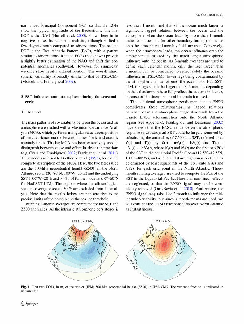
normalized Principal Component (PC), so that the EOFs

show the typical amplitude of the fluctuations. The first

EOF is the NAO (Hurrell et al. 2003), shown here in its

negative phase. Its pattern is realistic, although shifted a

few degrees north compared to observations. The second

EOF is the East Atlantic Pattern (EAP), with a pattern

similar to observations. Rotated EOFs (not shown) provide

a sightly better estimation of the NAO and shift the geo-

potential anomalies southward. However, for simplicity,

we only show results without rotation. The overall atmo-

spheric variability is broadly similar to that of IPSL-CM4

(Msadek and Frankignoul 2009).

3 SST influence onto atmosphere during the seasonal

cycle

3.1 Method

The main patterns of covariability between the ocean and the

atmosphere are studied with a Maximum Covariance Anal-

ysis (MCA), which performs a singular value decomposition

of the covariance matrix between atmospheric and oceanic

anomaly fields. The lag MCA has been extensively used to

distinguish between cause and effect in air-sea interactions

(e.g. Czaja and Frankignoul 2002; Frankignoul et al. 2011).

The reader is referred to Bretherton et al. (1992), for a more

complete description of the MCA. Here, the two fields used

are the 500-hPa geopotential height (Z500) in the North

Atlantic sector (20–80�N, 100�W–20�E) and the underlying

SST (100�W–20�E and 0�–70�N for the model and 0�–60�N

for HadISST-LIM). The regions where the climatological

sea-ice coverage exceeds 50 % are excluded from the anal-

ysis. Note that the results below are not sensitive to the

precise limits of the domain and the sea-ice threshold.

Running 3-month averages are computed for the SST and

Z500 anomalies. As the intrinsic atmospheric persistence is

less than 1 month and that of the ocean much larger, a

significant lagged relation between the ocean and the

atmosphere when the ocean leads by more than 1 month

indicates an oceanic (or other boundary forcing) influence

onto the atmosphere, if monthly fields are used. Conversely,

when the atmosphere leads, the ocean influence onto the

atmosphere is masked by the much larger atmospheric

influence onto the ocean. As 3-month averages are used to

define each calendar month, only the lags larger than

3 months can be considered to reflect solely the oceanic

influence in IPSL-CM5, lower lags being contaminated by

the atmospheric influence onto the ocean. For HadISST-

LIM, the lags should be larger than 3–5 months, depending

on the calendar month, to fully reflect the oceanic influence,

because of the linear temporal interpolation used.

The additional atmospheric persistence due to ENSO

complicates these relationships, as lagged relations

between ocean and atmosphere might also result from the

remote ENSO teleconnection onto the North Atlantic

region (see Appendix). Frankignoul and Kestenare (2002)

have shown that the ENSO influence on the atmospheric

response to extratropical SST could be largely removed by

substituting the anomalies of Z500 and SST, referred to as

Z(t) and T(t), by Z(t) - aN1(t) - bN2(t) and T(t) -

cN1(t) - dN2(t), where N1(t) and N2(t) are the first two PCs

of the SST in the equatorial Pacific Ocean (12.5�S–12.5�N,

100�E–80�W), and a, b, c and d are regression coefficients

determined by least square fits of the SST onto N1(t) and

N2(t), for each grid point in the North Atlantic. Three-

month running averages are used to compute the PCs of the

SST in the Equatorial Pacific. Note that non-linear effects

are neglected, so that the ENSO signal may not be com-

pletely removed (OrtizBevia et al. 2010). Furthermore, the

ENSO signal may take 1 or 2 month to influence the mid-

latitude variability, but since 3-month means are used, we

will consider the ENSO teleconnection over North Atlantic

as instantaneous.

Fig. 1 First two EOFs, in m, of the winter (JFM) 500-hPa geopotential height (Z500) in IPSL-CM5. The variance fraction is indicated in

parentheses

G. Gastineau et al.

123

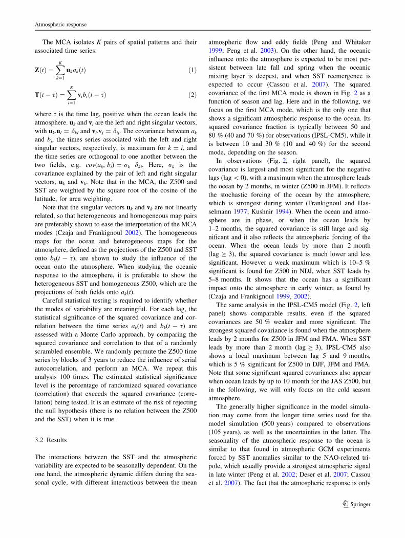
The MCA isolates K pairs of spatial patterns and their

associated time series:

ZðtÞ ¼XK

k¼1

ukakðtÞ ð1Þ

Tðt � sÞ ¼XK

i¼1

vibiðt � sÞ ð2Þ

where s is the time lag, positive when the ocean leads the

atmosphere. uk and vi are the left and right singular vectors,

with uk.ul = dkl and vi.vj = dij. The covariance between ak

and bi, the times series associated with the left and right

singular vectors, respectively, is maximum for k = i, and

the time series are orthogonal to one another between the

two fields, e.g. cov(ak, bi) = rk dki. Here, rk is the

covariance explained by the pair of left and right singular

vectors, uk and vk. Note that in the MCA, the Z500 and

SST are weighted by the square root of the cosine of the

latitude, for area weighting.

Note that the singular vectors uk and vk are not linearly

related, so that heterogeneous and homogeneous map pairs

are preferably shown to ease the interpretation of the MCA

modes (Czaja and Frankignoul 2002). The homogeneous

maps for the ocean and heterogeneous maps for the

atmosphere, defined as the projections of the Z500 and SST

onto bk(t - s), are shown to study the influence of the

ocean onto the atmosphere. When studying the oceanic

response to the atmosphere, it is preferable to show the

heterogeneous SST and homogeneous Z500, which are the

projections of both fields onto ak(t).

Careful statistical testing is required to identify whether

the modes of variability are meaningful. For each lag, the

statistical significance of the squared covariance and cor-

relation between the time series ak(t) and bk(t - s) are

assessed with a Monte Carlo approach, by comparing the

squared covariance and correlation to that of a randomly

scrambled ensemble. We randomly permute the Z500 time

series by blocks of 3 years to reduce the influence of serial

autocorrelation, and perform an MCA. We repeat this

analysis 100 times. The estimated statistical significance

level is the percentage of randomized squared covariance

(correlation) that exceeds the squared covariance (corre-

lation) being tested. It is an estimate of the risk of rejecting

the null hypothesis (there is no relation between the Z500

and the SST) when it is true.

3.2 Results

The interactions between the SST and the atmospheric

variability are expected to be seasonally dependent. On the

one hand, the atmospheric dynamic differs during the sea-

sonal cycle, with different interactions between the mean

atmospheric flow and eddy fields (Peng and Whitaker

1999; Peng et al. 2003). On the other hand, the oceanic

influence onto the atmosphere is expected to be most per-

sistent between late fall and spring when the oceanic

mixing layer is deepest, and when SST reemergence is

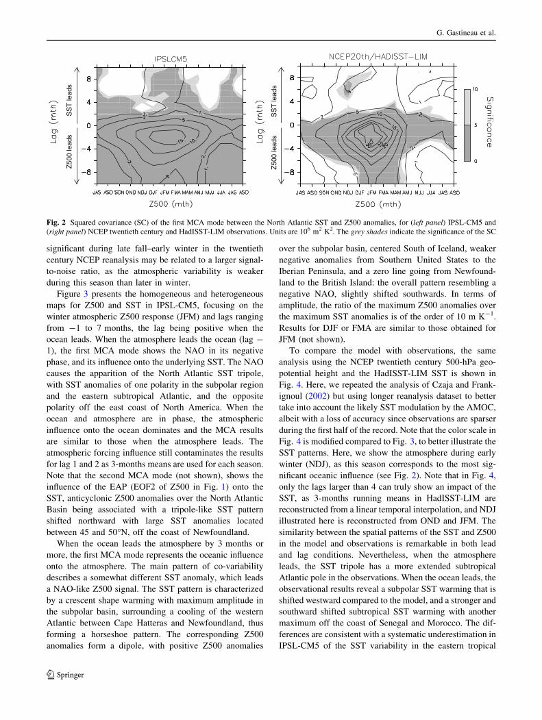
expected to occur (Cassou et al. 2007). The squared

covariance of the first MCA mode is shown in Fig. 2 as a

function of season and lag. Here and in the following, we

focus on the first MCA mode, which is the only one that

shows a significant atmospheric response to the ocean. Its

squared covariance fraction is typically between 50 and

80 % (40 and 70 %) for observations (IPSL-CM5), while it

is between 10 and 30 % (10 and 40 %) for the second

mode, depending on the season.

In observations (Fig. 2, right panel), the squared

covariance is largest and most significant for the negative

lags (lag \ 0), with a maximum when the atmosphere leads

the ocean by 2 months, in winter (Z500 in JFM). It reflects

the stochastic forcing of the ocean by the atmosphere,

which is strongest during winter (Frankignoul and Has-

selmann 1977; Kushnir 1994). When the ocean and atmo-

sphere are in phase, or when the ocean leads by

1–2 months, the squared covariance is still large and sig-

nificant and it also reflects the atmospheric forcing of the

ocean. When the ocean leads by more than 2 month

(lag C 3), the squared covariance is much lower and less

significant. However a weak maximum which is 10–5 %

significant is found for Z500 in NDJ, when SST leads by

5–8 months. It shows that the ocean has a significant

impact onto the atmosphere in early winter, as found by

(Czaja and Frankignoul 1999, 2002).

The same analysis in the IPSL-CM5 model (Fig. 2, left

panel) shows comparable results, even if the squared

covariances are 50 % weaker and more significant. The

strongest squared covariance is found when the atmosphere

leads by 2 months for Z500 in JFM and FMA. When SST

leads by more than 2 month (lag C 3), IPSL-CM5 also

shows a local maximum between lag 5 and 9 months,

which is 5 % significant for Z500 in DJF, JFM and FMA.

Note that some significant squared covariances also appear

when ocean leads by up to 10 month for the JAS Z500, but

in the following, we will only focus on the cold season

atmosphere.

The generally higher significance in the model simula-

tion may come from the longer time series used for the

model simulation (500 years) compared to observations

(105 years), as well as the uncertainties in the latter. The

seasonality of the atmospheric response to the ocean is

similar to that found in atmospheric GCM experiments

forced by SST anomalies similar to the NAO-related tri-

pole, which usually provide a strongest atmospheric signal

in late winter (Peng et al. 2002; Deser et al. 2007; Cassou

et al. 2007). The fact that the atmospheric response is only

Atmospheric response

123

significant during late fall–early winter in the twentieth

century NCEP reanalysis may be related to a larger signal-

to-noise ratio, as the atmospheric variability is weaker

during this season than later in winter.

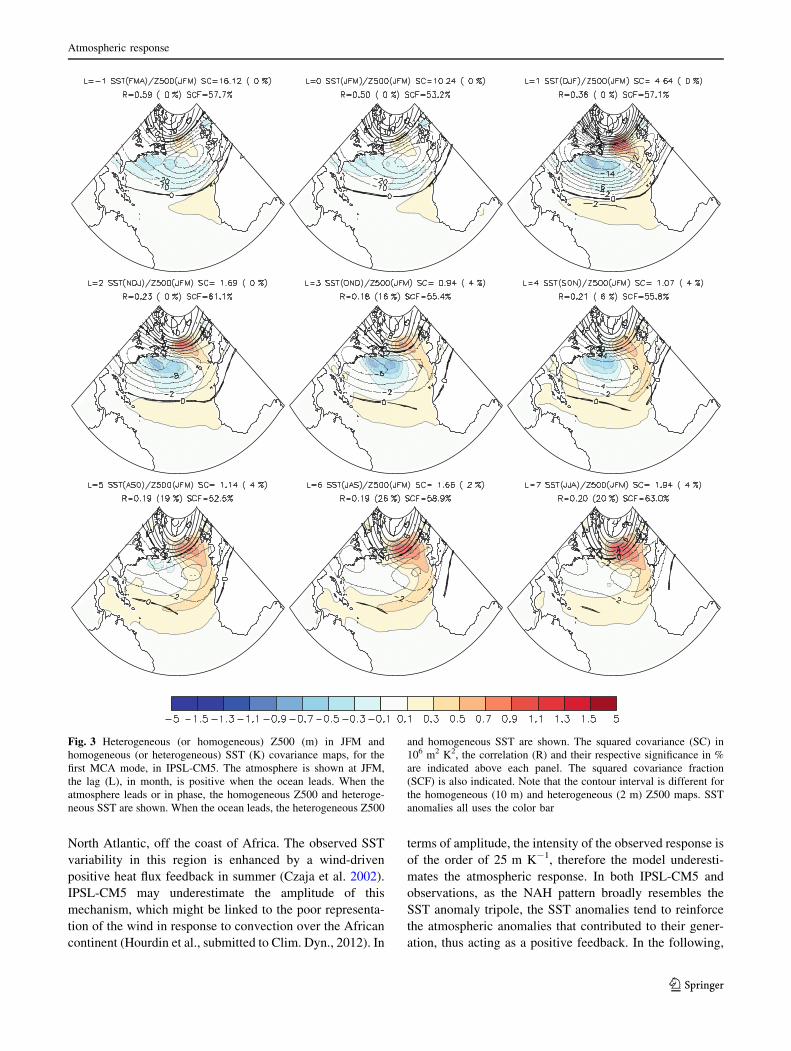
Figure 3 presents the homogeneous and heterogeneous

maps for Z500 and SST in IPSL-CM5, focusing on the

winter atmospheric Z500 response (JFM) and lags ranging

from -1 to 7 months, the lag being positive when the

ocean leads. When the atmosphere leads the ocean (lag -

1), the first MCA mode shows the NAO in its negative

phase, and its influence onto the underlying SST. The NAO

causes the apparition of the North Atlantic SST tripole,

with SST anomalies of one polarity in the subpolar region

and the eastern subtropical Atlantic, and the opposite

polarity off the east coast of North America. When the

ocean and atmosphere are in phase, the atmospheric

influence onto the ocean dominates and the MCA results

are similar to those when the atmosphere leads. The

atmospheric forcing influence still contaminates the results

for lag 1 and 2 as 3-months means are used for each season.

Note that the second MCA mode (not shown), shows the

influence of the EAP (EOF2 of Z500 in Fig. 1) onto the

SST, anticyclonic Z500 anomalies over the North Atlantic

Basin being associated with a tripole-like SST pattern

shifted northward with large SST anomalies located

between 45 and 50�N, off the coast of Newfoundland.

When the ocean leads the atmosphere by 3 months or

more, the first MCA mode represents the oceanic influence

onto the atmosphere. The main pattern of co-variability

describes a somewhat different SST anomaly, which leads

a NAO-like Z500 signal. The SST pattern is characterized

by a crescent shape warming with maximum amplitude in

the subpolar basin, surrounding a cooling of the western

Atlantic between Cape Hatteras and Newfoundland, thus

forming a horseshoe pattern. The corresponding Z500

anomalies form a dipole, with positive Z500 anomalies

over the subpolar basin, centered South of Iceland, weaker

negative anomalies from Southern United States to the

Iberian Peninsula, and a zero line going from Newfound-

land to the British Island: the overall pattern resembling a

negative NAO, slightly shifted southwards. In terms of

amplitude, the ratio of the maximum Z500 anomalies over

the maximum SST anomalies is of the order of 10 m K-1.

Results for DJF or FMA are similar to those obtained for

JFM (not shown).

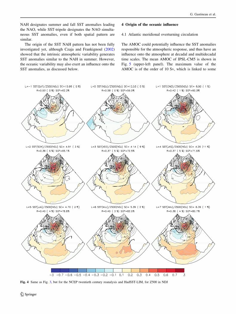
To compare the model with observations, the same

analysis using the NCEP twentieth century 500-hPa geo-

potential height and the HadISST-LIM SST is shown in

Fig. 4. Here, we repeated the analysis of Czaja and Frank-

ignoul (2002) but using longer reanalysis dataset to better

take into account the likely SST modulation by the AMOC,

albeit with a loss of accuracy since observations are sparser

during the first half of the record. Note that the color scale in

Fig. 4 is modified compared to Fig. 3, to better illustrate the

SST patterns. Here, we show the atmosphere during early

winter (NDJ), as this season corresponds to the most sig-

nificant oceanic influence (see Fig. 2). Note that in Fig. 4,

only the lags larger than 4 can truly show an impact of the

SST, as 3-months running means in HadISST-LIM are

reconstructed from a linear temporal interpolation, and NDJ

illustrated here is reconstructed from OND and JFM. The

similarity between the spatial patterns of the SST and Z500

in the model and observations is remarkable in both lead

and lag conditions. Nevertheless, when the atmosphere

leads, the SST tripole has a more extended subtropical

Atlantic pole in the observations. When the ocean leads, the

observational results reveal a subpolar SST warming that is

shifted westward compared to the model, and a stronger and

southward shifted subtropical SST warming with another

maximum off the coast of Senegal and Morocco. The dif-

ferences are consistent with a systematic underestimation in

IPSL-CM5 of the SST variability in the eastern tropical

Z50

0 le

ads

SS

T le

ads

Z50

0 le

ads

SS

T le

ads

Fig. 2 Squared covariance (SC) of the first MCA mode between the North Atlantic SST and Z500 anomalies, for (left panel) IPSL-CM5 and

(right panel) NCEP twentieth century and HadISST-LIM observations. Units are 106 m2 K2. The grey shades indicate the significance of the SC

G. Gastineau et al.

123

North Atlantic, off the coast of Africa. The observed SST

variability in this region is enhanced by a wind-driven

positive heat flux feedback in summer (Czaja et al. 2002).

IPSL-CM5 may underestimate the amplitude of this

mechanism, which might be linked to the poor representa-

tion of the wind in response to convection over the African

continent (Hourdin et al., submitted to Clim. Dyn., 2012). In

terms of amplitude, the intensity of the observed response is

of the order of 25 m K-1, therefore the model underesti-

mates the atmospheric response. In both IPSL-CM5 and

observations, as the NAH pattern broadly resembles the

SST anomaly tripole, the SST anomalies tend to reinforce

the atmospheric anomalies that contributed to their gener-

ation, thus acting as a positive feedback. In the following,

Fig. 3 Heterogeneous (or homogeneous) Z500 (m) in JFM and

homogeneous (or heterogeneous) SST (K) covariance maps, for the

first MCA mode, in IPSL-CM5. The atmosphere is shown at JFM,

the lag (L), in month, is positive when the ocean leads. When the

atmosphere leads or in phase, the homogeneous Z500 and heteroge-

neous SST are shown. When the ocean leads, the heterogeneous Z500

and homogeneous SST are shown. The squared covariance (SC) in

106 m2 K2, the correlation (R) and their respective significance in %

are indicated above each panel. The squared covariance fraction

(SCF) is also indicated. Note that the contour interval is different for

the homogeneous (10 m) and heterogeneous (2 m) Z500 maps. SST

anomalies all uses the color bar

Atmospheric response

123

NAH designates summer and fall SST anomalies leading

the NAO, while SST-tripole designates the NAO simulta-

neous SST anomalies, even if both spatial pattern are

similar.

The origin of the SST NAH pattern has not been fully

investigated yet, although Czaja and Frankignoul (2002)

showed that the intrinsic atmospheric variability generates

SST anomalies similar to the NAH in summer. However,

the oceanic variability may also exert an influence onto the

SST anomalies, as discussed below.

4 Origin of the oceanic influence

4.1 Atlantic meridional overturning circulation

The AMOC could potentially influence the SST anomalies

responsible for the atmospheric response, and thus have an

influence onto the atmosphere at decadal and multidecadal

time scales. The mean AMOC of IPSL-CM5 is shown in

Fig. 5 (upper-left panel). The maximum value of the

AMOC is of the order of 10 Sv, which is linked to some

Fig. 4 Same as Fig. 3, but for the NCEP twentieth century reanalysis and HadSST-LIM, for Z500 in NDJ

G. Gastineau et al.

123

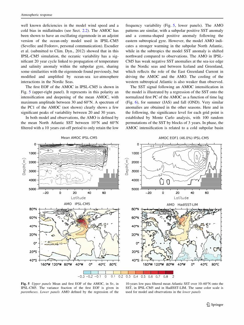
well known deficiencies in the model wind speed and a

cold bias in midlatitudes (see Sect. 2.2). The AMOC has

been shown to have an oscillating eigenmode in an adjoint

version of the ocean-only model used in IPSL-CM5

(Sevellec and Fedorov, personal communication). Escudier

et al. (submitted to Clim. Dyn., 2012) showed that in this

IPSL-CM5 simulation, the oceanic variability has a sig-

nificant 20 year cycle linked to propagation of temperature

and salinity anomaly within the subpolar gyre, sharing

some similarities with the eigenmode found previously, but

modified and amplified by ocean-sea ice-atmosphere

interactions in the Nordic Seas.

The first EOF of the AMOC in IPSL-CM5 is shown in

Fig. 5 (upper-right panel). It represents in this polarity an

intensification and deepening of the mean AMOC, with

maximum amplitude between 30 and 60�N. A spectrum of

the PC1 of the AMOC (not shown) clearly shows a few

significant peaks of variability between 20 and 30 years.

In both model and observations, the AMO is defined by

the mean North Atlantic SST between 10�N and 60�N

filtered with a 10 years cut-off period to only retain the low

frequency variability (Fig. 5, lower panels). The AMO

patterns are similar, with a subpolar positive SST anomaly

and a comma-shaped positive anomaly following the

eastern subtropical gyre. However, the model AMO indi-

cates a stronger warming in the subpolar North Atlantic,

while in the subtropics the model SST anomaly is shifted

northward compared to observations. The AMO in IPSL-

CM5 has weak negative SST anomalies at the sea-ice edge

in the Nordic seas and between Iceland and Greenland,

which reflects the role of the East Greenland Current in

driving the AMOC and the AMO. The cooling of the

western subtropical Atlantic is also weaker than observed.

The SST signal following an AMOC intensification in

the model is illustrated by a regression of the SST onto the

normalized first PC of the AMOC as a function of time lag

(Fig. 6), for summer (JAS) and fall (OND). Very similar

anomalies are obtained in the other seasons. Here and in

the following, the significance level for each grid point is

established by Monte Carlo analysis, with 100 random

permutations of the SST by blocks of 3 years. In phase, the

AMOC intensification is related to a cold subpolar basin

Fig. 5 Upper panels Mean and first EOF of the AMOC, in Sv, in

IPSL-CM5. The variance fraction of the first EOF is given in

parentheses. Lower panels AMO defined by the regression of the

10-years low pass filtered mean Atlantic SST over 10–60�N onto the

SST, in IPSL-CM5 and in HadISST-LIM. The same color scale is

used for model and observations in the lower panels

Atmospheric response

123

and a warm subtropical North Atlantic, in particular off the

coast of North America. The subpolar basin south of Ice-

land, where deep convection occurs in the model, is cold,

in part due to the mixing of the surface and deep waters

which took place a few years before the AMOC intensifi-

cation. As shown in Eden and Willebrand (2001); Desha-

yes and Frankignoul (2008); Gastineau and Frankignoul

(2011), most models show a negative AMOC anomaly in

the subpolar regions and a positive one in the subtropics as

a fast response to a positive NAO, consistent with the

anomalous Ekman pumping and the deep return flow dri-

ven by the NAO surface wind stress. The NAO also causes

the apparition of the North Atlantic SST tripole, through

the modification of the surface heat fluxes (see Figs. 3, 4).

After an AMOC intensification, the poleward heat transport

increases and a strong warming develops in the subpolar

basin. The positive SST anomalies are first located in the

North Atlantic current region, then propagate into the

subpolar region by lag 3, expanding and intensifying until

they reach a maximum at 9 years lag. At the same time, the

warming spreads in the subtropical gyre while cooling

occurs in the Gulf Stream region, so that the SST anomaly

forms a comma-shaped pattern in the North Atlantic. The

similarity between the AMOC-induced SST and the AMO

in the model is striking (compare lower-left panel of Fig. 5

and the lower panels of Fig. 6), as in most climate models

(Knight et al. 2005; Msadek and Frankignoul 2009), even

if the lag between the AMOC and AMO is model depen-

dent (Marini 2011).

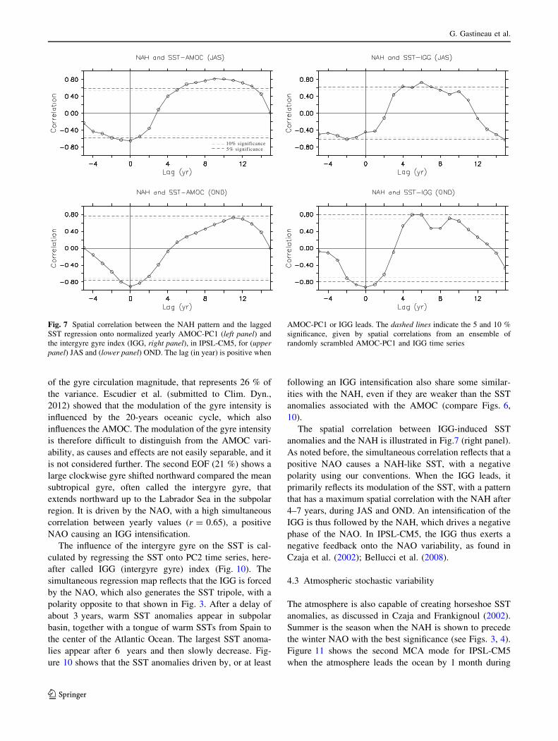
The AMOC-induced SSTs also have strong similarities

with the NAH pattern found in the MCA (compare with

Fig. 3, lag 6 or 7). In Fig. 7, we computed the spatial

correlation between the SSTs regressed onto AMOC-

PC1 at different lags in years and the SST NAH pattern,

which is given by the homogeneous SST map in Fig. 3

when the SST leads the JFM negative NAO by 3 months

(SST in OND) and 6 months (SST in JAS). The signifi-

cance of the spatial correlations are based on the 5 and

10 % strongest spatial correlations obtained in an ensemble

of 200 randomly scrambled AMOC time series, using

blocks of 3 years to account for autocorrelation.

In summer (JAS, Fig. 7, upper-left panel), the SST

patterns have a broad and significant positive spatial cor-

relation, which reaches its maximum 9 years after the

AMOC in summer (JAS), while a weaker negative corre-

lation is found in phase. The negative in phase correlation

is due to the NAO simultaneously influencing the SST and

the AMOC, as a negative phase of the NAO causes tripolar

SST anomalies that have similarities with the NAH, while

it weakly decreases the AMOC (Gastineau and Frankignoul

2011). On the other hand, as shown in Fig. 6, the SST is

progressively modulated by the currents associated with an

AMOC intensification until the SST anomaly reaches the

horseshoe-shape at lag 6–13 years that can optimally force

an atmospheric signal. In fall (OND, Fig. 7, lower-left

panel), a larger negative correlation is obtained in phase, as

the NAO is more active during this season. A weakly

significant positive correlation is still obtained when the

AMOC leads by 11 years, which indicates a weaker but

statistically significant AMOC influence onto the NAH.

The cold-season atmospheric response to the AMOC has

been discussed in Gastineau and Frankignoul (2011), who

showed that it was most significant when the AMOC leads

by 9 years in IPSL-CM5, with a negative phase of the

NAO following an AMOC intensification. The pathways of

the winter atmospheric response to the AMOC in IPSL-

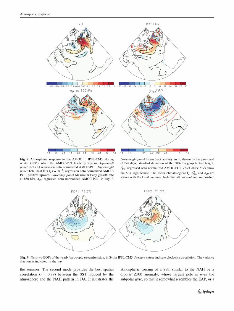
CM5 are presented for lag 9 in Fig. 8, with the regressions

onto the normalized AMOC-PC1 of the winter (JFM) SST,

heat flux, 850-hPa maximum Eady growth rate and

500-hPa transient eddy activity. Note that the storm track

intensity is calculated from daily outputs.

The SST anomalies in the North Atlantic modify the

heat exchanges between the ocean and the atmosphere,

the atmosphere acting as a negative feedback that damps

the SST anomalies as in Frankignoul and Kestenare (2002)

and Park et al. (2005). This increases the upward heat flux

in the southern subpolar basin, where the SST anomalies

are the largest, and decreases it further north. In the Gulf

Stream/North Atlantic Current region where the climato-

logical heat flux is maximum, the heat flux decreases to the

north and increases to the south, thus shifting the ocean

forcing southward. These changes contribute to the

decrease of the storm track intensity and shift the storm

track southward, as shown by the maximum Eady growth

rate at 850-hPa (Fig. 8, lower-left panel) and the 500-hPa

geopotential height standard deviation (Fig. 8, lower-right

panel), leading to a negative NAO phase. We suspect that it

is the reduction (amplification) of meridional SST gradient

in southern (northern) subpolar region, together with the

southward shift in the Gulf Stream/North Atlantic Current

region, which causes the overall decrease of the storm track

and the negative NAO response. The signal is similar in

IPSL-CM4, which was illustrated in Gastineau and

Frankignoul (2011), but the atmospheric response is

stronger and more significant in IPSL-CM5.

4.2 Atlantic gyre circulation

The mean gyre circulation of IPSL-CM5 shows a clock-

wise subtropical gyre centered at 30�N, and a counter-

clockwise subpolar gyre centered at 55�N (not shown). The

circulation within the subtropical gyre reaches 35 Sv,

which is comparable to observational estimates (Schott

et al. 1988). The first two EOFs of the barotropic stream-

function are shown in Fig. 9, positive values indicating

clockwise circulation. The first EOF indicates a modulation

G. Gastineau et al.

123

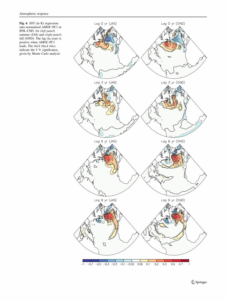
Fig. 6 SST (in K) regression

onto normalized AMOC-PC1 in

IPSL-CM5, for (left panel)summer (JAS) and (right panel)fall (OND). The lag (in year) is

positive when AMOC-PC1

leads. The thick black linesindicate the 5 % significance,

given by Monte Carlo analysis

Atmospheric response

123

of the gyre circulation magnitude, that represents 26 % of

the variance. Escudier et al. (submitted to Clim. Dyn.,

2012) showed that the modulation of the gyre intensity is

influenced by the 20-years oceanic cycle, which also

influences the AMOC. The modulation of the gyre intensity

is therefore difficult to distinguish from the AMOC vari-

ability, as causes and effects are not easily separable, and it

is not considered further. The second EOF (21 %) shows a

large clockwise gyre shifted northward compared the mean

subtropical gyre, often called the intergyre gyre, that

extends northward up to the Labrador Sea in the subpolar

region. It is driven by the NAO, with a high simultaneous

correlation between yearly values (r = 0.65), a positive

NAO causing an IGG intensification.

The influence of the intergyre gyre on the SST is cal-

culated by regressing the SST onto PC2 time series, here-

after called IGG (intergyre gyre) index (Fig. 10). The

simultaneous regression map reflects that the IGG is forced

by the NAO, which also generates the SST tripole, with a

polarity opposite to that shown in Fig. 3. After a delay of

about 3 years, warm SST anomalies appear in subpolar

basin, together with a tongue of warm SSTs from Spain to

the center of the Atlantic Ocean. The largest SST anoma-

lies appear after 6 years and then slowly decrease. Fig-

ure 10 shows that the SST anomalies driven by, or at least

following an IGG intensification also share some similar-

ities with the NAH, even if they are weaker than the SST

anomalies associated with the AMOC (compare Figs. 6,

10).

The spatial correlation between IGG-induced SST

anomalies and the NAH is illustrated in Fig.7 (right panel).

As noted before, the simultaneous correlation reflects that a

positive NAO causes a NAH-like SST, with a negative

polarity using our conventions. When the IGG leads, it

primarily reflects its modulation of the SST, with a pattern

that has a maximum spatial correlation with the NAH after

4–7 years, during JAS and OND. An intensification of the

IGG is thus followed by the NAH, which drives a negative

phase of the NAO. In IPSL-CM5, the IGG thus exerts a

negative feedback onto the NAO variability, as found in

Czaja et al. (2002); Bellucci et al. (2008).

4.3 Atmospheric stochastic variability

The atmosphere is also capable of creating horseshoe SST

anomalies, as discussed in Czaja and Frankignoul (2002).

Summer is the season when the NAH is shown to precede

the winter NAO with the best significance (see Figs. 3, 4).

Figure 11 shows the second MCA mode for IPSL-CM5

when the atmosphere leads the ocean by 1 month during

5% significance10% significance

Fig. 7 Spatial correlation between the NAH pattern and the lagged

SST regression onto normalized yearly AMOC-PC1 (left panel) and

the intergyre gyre index (IGG, right panel), in IPSL-CM5, for (upperpanel) JAS and (lower panel) OND. The lag (in year) is positive when

AMOC-PC1 or IGG leads. The dashed lines indicate the 5 and 10 %

significance, given by spatial correlations from an ensemble of

randomly scrambled AMOC-PC1 and IGG time series

G. Gastineau et al.

123

the summer. The second mode provides the best spatial

correlation (r = 0.79) between the SST induced by the

atmosphere and the NAH pattern in JJA. It illustrates the

atmospheric forcing of a SST similar to the NAH by a

dipolar Z500 anomaly, whose largest pole is over the

subpolar gyre, so that it somewhat resembles the EAP, or a

Fig. 8 Atmospheric response to the AMOC in IPSL-CM5, during

winter (JFM), when the AMOC-PC1 leads by 9 years. Upper-leftpanel SST (K) regression onto normalized AMOC-PC1. Upper-rightpanel Total heat flux Q (W m-1) regression onto normalized AMOC-

PC1, positive upward. Lower-left panel Maximum Eady growth rate

at 850-hPa, rBI, regressed onto normalized AMOC-PC1, in day-1.

Lower-right panel Storm track activity, in m, shown by the pass-band

(2.2–5 days) standard deviation of the 500-hPa geopotential height,

z02500, regressed onto normalized AMOC-PC1. Thick black lines show

the 5 % significance. The mean climatological Q, z02500 and rBI are

shown with thick red contours. Note that all red contours are positive

Fig. 9 First two EOFs of the yearly barotropic streamfunction, in Sv, in IPSL-CM5. Positive values indicate clockwise circulation. The variance

fraction is indicated in the top

Atmospheric response

123

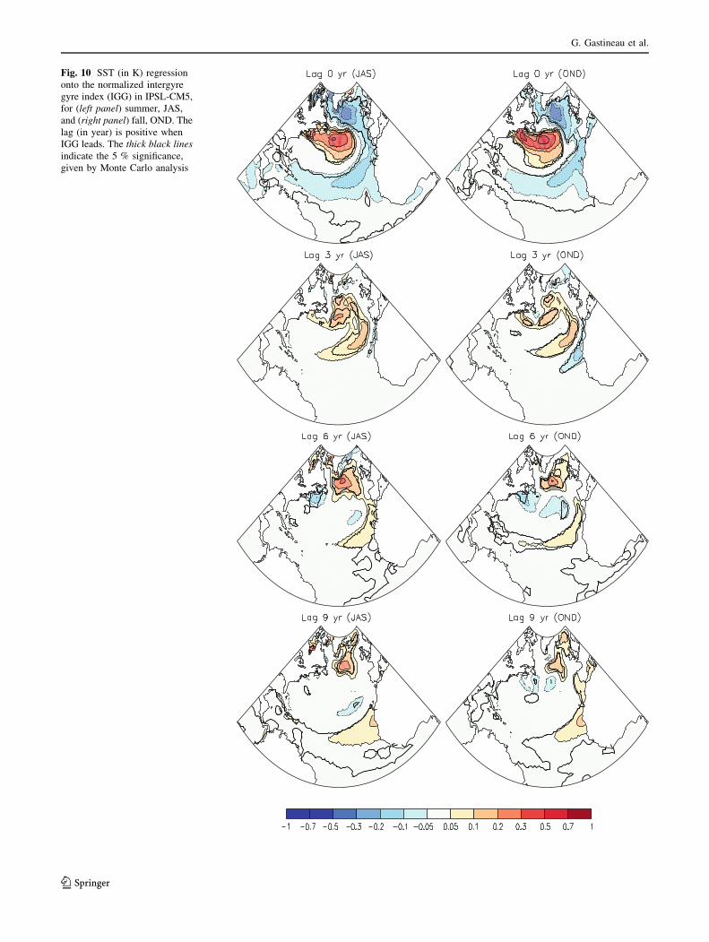
Fig. 10 SST (in K) regression

onto the normalized intergyre

gyre index (IGG) in IPSL-CM5,

for (left panel) summer, JAS,

and (right panel) fall, OND. The

lag (in year) is positive when

IGG leads. The thick black linesindicate the 5 % significance,

given by Monte Carlo analysis

G. Gastineau et al.

123

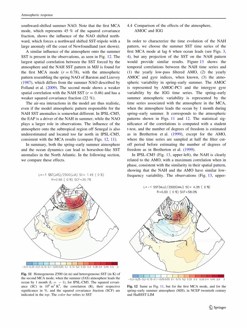
southward-shifted summer NAO. Note that the first MCA

mode, which represents 45 % of the squared covariance

fraction, shows the influence of the NAO shifted north-

ward, which forces a northward shifted SST-tripole with a

large anomaly off the coast of Newfoundland (not shown).

A similar influence of the atmosphere onto the summer

SST is present in the observations, as seen in Fig. 12. The

largest spatial correlation between the SST forced by the

atmosphere and the NAH SST pattern in MJJ is found for

the first MCA mode (r = 0.78), with the atmospheric

pattern resembling the spring NAO of Barston and Lizevey

(1987), which differs from the summer NAO described by

Folland et al. (2009). The second mode shows a weaker

spatial correlation with the NAH SST (r = 0.46) and has a

weaker squared covariance fraction (22 %).

The air-sea interactions in the model are thus realistic,

even if the model atmospheric pattern responsible for the

NAH SST anomalies is somewhat different. In IPSL-CM5,

the EAP is a driver of the NAH in summer, while the NAO

plays a larger role in observations. The influence of the

atmosphere onto the subtropical region off Senegal is also

underestimated and located too far north in IPSL-CM5,

consistent with the MCA results (compare Figs. 12, 11).

In summary, both the spring–early summer atmosphere

and the ocean dynamics can lead to horseshoe-like SST

anomalies in the North Atlantic. In the following section,

we compare these effects.

4.4 Comparison of the effects of the atmosphere,

AMOC and IGG

In order to characterize the time evolution of the NAH

pattern, we choose the summer SST time series of the

first MCA mode at lag 6 when ocean leads (see Figs. 3,

4), but any projection of the SST on the NAH pattern

would provide similar results. Figure 13 shows the

temporal correlations between the NAH time series and

(1) the yearly low-pass filtered AMO, (2) the yearly

AMOC and gyre indices, when known, (3) the atmo-

spheric variability in spring–early summer. The AMOC

is represented by AMOC-PC1 and the intergyre gyre

variability by the IGG time series. The spring–early

summer atmospheric variability is represented by the

time series associated with the atmosphere in the MCA,

when the atmosphere leads the ocean by 1 month during

spring–early summer. It corresponds to the atmospheric

patterns shown in Figs. 11 and 12. The statistical sig-

nificance of the correlations is computed with a student

t-test, and the number of degrees of freedom is estimated

as in Bretherton et al. (1999), except for the AMO,

where the time series are sampled at half the filter cut-

off period before estimating the number of degrees of

freedom as in Bretherton et al. (1999).

In IPSL-CM5 (Fig. 13, upper-left), the NAH is clearly

related to the AMO, with a maximum correlation when in

phase, consistent with the similarity in their spatial pattern,

showing that the NAH and the AMO have similar low-

frequency variability. The observations (Fig. 13, upper-

Fig. 11 Homogeneous Z500 (in m) and heterogeneous SST (in K) of

the second MCA mode, when the summer (JAS) atmosphere leads the

ocean by 1 month (L = - 1), for IPSL-CM5. The squared covari-

ance (SC) in 106 m2 K2, the correlation (R), their respective

significance in %, and the squared covariance fraction (SCF) are

indicated in the top. The color bar refers to SST

Fig. 12 Same as Fig. 11, but for the first MCA mode, and for the

spring–early summer atmosphere (MJJ), in NCEP twentieth century

and HadISST-LIM

Atmospheric response

123

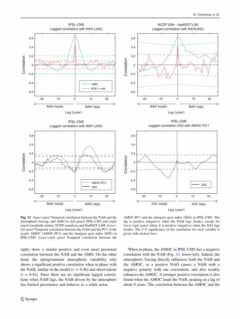
right) show a similar positive and even more persistent

correlation between the NAH and the AMO. On the other

hand, the spring/summer atmospheric variability only

shows a significant positive correlation when in phase with

the NAH, similar in the model (r = 0.46) and observations

(r = 0.42). Since there are no significant lagged correla-

tions when NAH lags, the NAH driven by the atmosphere

has limited persistence and behaves as a white noise.

When in phase, the AMOC in IPSL-CM5 has a negative

correlation with the NAH (Fig. 13, lower-left). Indeed, the

atmospheric forcing directly influences both the NAH and

the AMOC, as a positive NAO causes a NAH with a

negative polarity with our convention, and also weakly

enhances the AMOC. A stronger positive correlation is also

found when the AMOC leads the NAH, peaking at a lag of

about 9 years. The correlation between the AMOC and the

-20 -10 0 10 20

-0.6

-0.4

-0.2

0

0.2

0.4

0.6

Cor

rela

tion

-20 -10 0 10 20

-0.6

-0.4

-0.2

0

0.2

0.4

0.6

Cor

rela

tion

-20 -10 0 10 20

-0.6

-0.4

-0.2

0

0.2

0.4

0.6

Cor

rela

tion

-20 -10 0 10 20

-0.6

-0.4

-0.2

0

0.2

0.4

0.6

Cor

rela

tion

AMO

ATM -1 mth

IGG

AMOC-PC1IGG

Fig. 13 Upper panel Temporal correlation between the NAH and the

atmospheric forcing, and AMO in (left panel) IPSL-CM5 and (rightpanel) twentieth century NCEP reanalysis and HadISST-LIM. Lower-left panel Temporal correlation between the NAH and the PC1 of the

yearly AMOC (AMOC-PC1) and the intergyre gyre index (IGG) in

IPSL-CM5. Lower-right panel Temporal correlation between the

AMOC-PC1 and the intergyre gyre index (IGG) in IPSL-CM5. The

lag is positive (negative) when the NAH lags (leads), except for

lower-right panel where it is positive (negative) when the IGG lags

(leads). The 5 % significance of the correlation for each variable is

given with dashed lines

G. Gastineau et al.

123

NAH remains significant from lag 5 to lag 13, reflecting a

rather low-frequency influence. Since the NAH influences

the NAO, this confirms that the low-frequency variability

of the AMOC has an impact onto the atmosphere, as shown

by Gastineau and Frankignoul (2011). A significant nega-

tive correlation is also seen when the AMOC leads the

NAH by about 20 years, reflecting the change of phase

associated with the strong 20-years cycle of the AMOC.

The IGG index also shows significant links with the

NAH in IPSL-CM5, with a negative correlation while in

phase and positive correlation when the IGG leads by a time

lag between 4 and 9 years. There is also a significant neg-

ative correlation when the IGG leads by 15–23 years, which

presumably also reflects the 20-years periodicity that is seen

in many oceanic variables in IPSL-CM5. To briefly docu-

ment the links between the IGG and the AMOC, Fig. 13

(lower-right) shows the temporal correlation between

AMOC-PC1 and IGG. The IGG precedes the AMOC by

3–11 years, which is consistent with the 5-years lag

between the subpolar influence on the IGG and the AMOC

discussed in Escudier et al. (submitted to Clim. Dyn., 2012).

No significant correlation is found when the AMOC leads,

so that the delayed effects of the AMOC (lag 9) and that of

IGG (lag 5) are well distinct. Since the lag correlation with

the AMOC is substantially larger than with the IGG, the

AMOC effects seems to dominate the effect of the IGG.

5 Discussion and conclusion

The ocean-atmosphere coupling in the North Atlantic

region is investigated in the IPSL-CM5 model and obser-

vations with a MCA between the SST and the 500-hPa

geopotential height. The model results are compared to

observations of the twentieth century, after the global

warming pattern is removed using a linear inverse model-

ing method. In both model and observations, the main

patterns of covariability are given by the NAO and the SST

tripole when the atmosphere leads, and by similar NAH

SST and NAO-like patterns when the ocean leads. The SST

influence is twice weaker in IPSL-CM5, but it is significant

during the whole cold season, while the SST influence is

only detected during early winter for the observations,

which may, in part, reflects the longer sample in the model

and the observational uncertainties. Both in IPSL-CM5 and

the observations, the SST anomalies exert a positive

feedback on the NAO variability since the tripole and the

NAH patterns are rather similar. The NAH pattern in the

observation has been related to the stochastic variability of

the atmosphere during summer (Czaja and Frankignoul

2002). Here, we show that the NAH pattern also has a

significant decadal and multidecadal variability, which is

closely related to the AMO.

In the IPSL-CM5 model, an AMOC intensification

causes an increase of the northward oceanic heat transport,

which warms the temperatures in the North Atlantic region.

Therefore, the AMOC, which largely drives the AMO, is

also a driver of the NAH, the AMOC leading both the NAH

and the AMO by 9 years. As the summer NAH is followed

in winter by an atmospheric response resembling a nega-

tive NAO phase, the AMOC-induced warming has a sig-

nificant impact on the winter NAO activity, favoring a

negative NAO state as found by Gastineau and Frankignoul

(2011). The AMOC was also found to be a main driver of

the AMO in other climate models (e.g. Knight et al. 2005;

Danabasoglu 2008; Marini 2011). Therefore, we suggest a

possible influence of the AMOC onto the NAH and NAO

during the twentieth century, although no direct AMOC

observations are available to verify such link. Since the

AMOC may be predictable up to a decade ahead (Collins

et al. 2006), the AMOC influence onto the NAO implies a

potential decadal predictability of the NAO. This may

explain the predictability found over the North Atlantic

region in the decadal forecast experiments (Pohlmann et al.

2006; Keenlyside et al. 2008; Teng et al. 2011).

The AMOC is a two dimensional view of a more

complex three dimensional oceanic circulation, and the

meridional overturning is not the only process that influ-

ences the NAH even though it appears to be the dominant

one. In IPSL-CM5, an intergyre gyre that is forced by the

NAO also explains part of the NAH SST anomalies, sim-

ilarly to the studies of Czaja and Marshall (2001) and

Bellucci et al. (2008). Interestingly, the intergyre gyre

leads to a delayed damping of the SST anomalies that are

directly generated by the NAO, with a delay of 4–9 years,

which is consistent with the time scale of Rossby wave

propagation through the Atlantic Basin. The water-mass

pathways and their influence on SST need further investi-

gations to reveal the processes involved in the AMOC and

gyre circulation and their links.

The sea ice may also play a role in the coupling between

ocean and atmosphere. Previous studies suggest that sea ice

variability acts as a negative feedback on the NAO, as the

sea-ice anomaly pattern driven by a positive NAO tends to

generate a negative NAO-like atmospheric response

(Magnusdottir et al. 2004; Deser et al. 2007; Strong et al.

2009). As the sea-ice extension is too large is IPSL-CM5,

the sea-ice variations take place in unrealistic locations and

their impact should be different. Gastineau and Frankig-

noul (2011) suggested that the AMOC primarily influences

the atmosphere in the model via SST changes, not sea-ice

changes, but the issue requires further studies.

The IPSL-CM5 simulation presented in this study uses a

low resolution. Chelton and Xie (2010) have shown that

low-resolution atmospheric GCMs strongly underestimate

the ocean-atmosphere coupling due to the poor

Atmospheric response

123

representation of SST fronts and their impact onto the

atmosphere. This may explain in part the low sensitivity of

the model response compared to the observations. A better

understanding of the ocean-atmosphere interactions is

needed as the resolution of the models increases.

Acknowledgments The research leading to these results has

received funding from the European Community’s 7th framework

programme (FP7/2007-2013) under grant agreement No. GA212643

(THOR: ‘‘Thermohaline Overturning—at Risk’’, 2008-2012). We are

grateful to C. Marini who provided the HadISST-LIM data. We also

thank J. Mignot, D. Swingedouw and two anonymous reviewers for

their useful comments and suggestions.

Appendix: The removal of ENSO from North Atlantic

SST and geopotential height

The variability of ENSO is assessed using the first two PCs

of the SST in the equatorial Pacific Ocean (12.5�S–12.5�N,

100�E–80�W). The first (second) modes represent between

62 and 66 % (7 and 11 %) of the total variance depending

on the season. The ENSO variability is rather low in IPSL-

CM5, with an incorrect phase locking of the ENSO vari-

ability to the annual cycle, even if its frequency spectrum is

relatively similar to that of the observations.

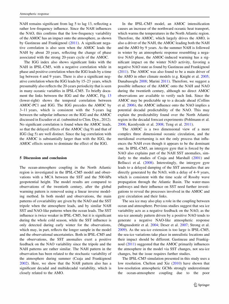
Here, the relations between ENSO and the North

Atlantic variability are assessed using simultaneous

regressions of the SST (K) and Z500 (m) onto the first

normalized PC of the Equatorial Pacific SST. In observa-

tions (Fig. 14), the main ENSO effect is to shift the sub-

tropical jets equatorwards during El Nino phase, thereby

inducing the same SST anomalies as a negative NAO in the

Atlantic subtropical domain (Seager et al. 2003), while the

subpolar North Atlantic SST anomalies are much weaker

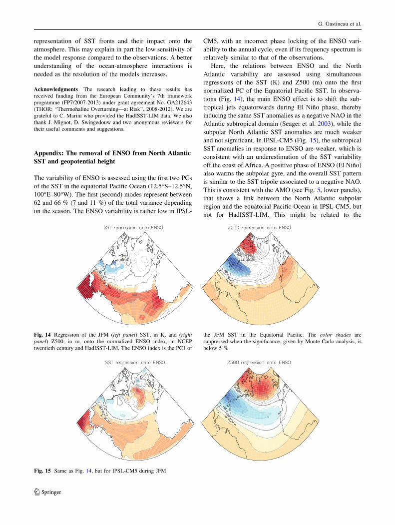
and not significant. In IPSL-CM5 (Fig. 15), the subtropical

SST anomalies in response to ENSO are weaker, which is

consistent with an underestimation of the SST variability

off the coast of Africa. A positive phase of ENSO (El Nino)

also warms the subpolar gyre, and the overall SST pattern

is similar to the SST tripole associated to a negative NAO.

This is consistent with the AMO (see Fig. 5, lower panels),

that shows a link between the North Atlantic subpolar

region and the equatorial Pacific Ocean in IPSL-CM5, but

not for HadISST-LIM. This might be related to the

Fig. 14 Regression of the JFM (left panel) SST, in K, and (rightpanel) Z500, in m, onto the normalized ENSO index, in NCEP

twentieth century and HadISST-LIM. The ENSO index is the PC1 of

the JFM SST in the Equatorial Pacific. The color shades are

suppressed when the significance, given by Monte Carlo analysis, is

below 5 %

Fig. 15 Same as Fig. 14, but for IPSL-CM5 during JFM

G. Gastineau et al.

123

incorrect phase locking of ENSO, which was demonstrated

to alter the teleconnection with the Equatorial Pacific.

The winter Z500 related to ENSO SST anomalies has

strong anomalies over North America, as the Pacific-North

American pattern is strongly modulated by ENSO. Over

the North Atlantic the Z500 anomalies are roughly similar

to the NAO, an El Nino phase causing a negative phase of

the NAO in both model and observation as in Alexander

and Scott (2002). The anomalies are also similar to those of

OrtizBevia et al. (2010), but the strong non-linearity of the

ENSO teleconnections is neglected in this study.

In both the model and observations, ENSO has an

impact onto SST and Z500 similar to the local influence of

SST anomalies (compare Figs. 14 and 15 with Figs. 3 and

4, for lags larger than 3–4 months). Unlike in the obser-

vations of Frankignoul and Kestenare (2005), the removal

of ENSO turned out to reduce the statistical significance of

squared covariance and correlation of the first MCA mode

when the ocean leads compared to other studies Czaja and

Frankignoul (1999); Czaja and Frankignoul (2002), where

ENSO was not removed from the SST and Z500. For

example, when ENSO is not removed in observations, the

squared covariance of the first MCA mode is 5 % signifi-

cant up to lag 6 months when the ocean leads for Z500 in

FMA, while the statistical significance is similar for Z500

in NDJ.

References

Alexander M, Scott J (2002) The influence of ENSO on air-sea

interaction in the Atlantic. Geophys Res Lett 29(14):46. doi:

10.1029/2001GL014347

Barston AG, Lizevey RE (1987) Classification, seasonality and

persistence of low-frequency atmospheric circulation patterns.

Mon Wea Rev 115:1083–1126

Bellucci A, Gualdi S, Scoccimarro E, Navarra A (2008) NAO-ocean

circulation interactions in a coupled general circulation model.

Clim Dyn 31(7):759–777

Bretherton C, Widmann M, Dymnikov V, Wallace J, Blade I (1999)

The effective number of spatial degrees of freedom of a time-

varying field. J Climate 12(7):1990–2009

Bretherton CS, Smith C, Wallace JM (1992) An intercomparison of

methods for finding coupled patterns in climate data. J Climate

5(6):541–560

Cassou C, Deser C, Alexander MA (2007) Investigating the impact of

reemerging sea surface temperature anomalies on the winter

atmospheric circulation over the North Atlantic. J Climate

20(14):3510–3526

Cayan DR (1992) Latent and sensible heat flux anomalies over the

northern oceans: the connection to monthly atmospheric circu-

lation. J Climate 5(4):354–369

Chelton D, Xie S-P (2010) Coupled ocean-atmosphere interaction at

oceanic mesoscales. Oceanography 23(4):52–69

Collins M et al (2006) Interannual to decadal climate predictability in

the North Atlantic: a multimodel-ensemble study. J Climate

19(7):1195–1203

Compo GP, Sardeshmukh PD (2010) Removing ENSO-related

variations from the climate record. J Climate 23(8):1957–1978

Compo GP et al (2011) The twentieth century reanalysis project. Q J

R Meteorol Soc 137(654):1–28

Cunningham SA et al (2007) Temporal variability of the Atlantic

meridional overturning circulation at 26.5N. Science 317(5840):

935–938

Czaja A, Frankignoul C (1999) Influence of the North Atlantic SST

on the atmospheric circulation. Geophys Res Lett 26:2969–2972

Czaja A, Frankignoul C (2002) Observed impact of Atlantic SST

anomalies on the North Atlantic oscillation. J Climate 15(6):606–

623

Czaja A, Marshall J (2001) Observations of atmosphere-ocean

coupling in the North Atlantic. Q J R Meteorol Soc

127:1893–1916

Czaja A, van der Vaart P, Marshall J (2002) A diagnostic study of the

role of remote forcing in tropical Atlantic variability. J Climate

15(22):3280–3290

Danabasoglu G (2008) On multidecadal variability of the Atlantic

meridional overturning circulation in the community climate

system model version 3. J Climate 21(21):5524–5544

D’Andrea F, Czaja A, Marshall J (2005) Impact of anomalous ocean

heat transport on the North Atlantic oscillation. J Climate

18(23):4955–4969

Delworth TL, Greatbatch RJ (2000) Multidecadal thermohaline

circulation variability driven by atmospheric surface flux forc-

ing. J Climate 13(9):1481–1495

Deser C, Alexander MA, Xie S, Phillips AS (2009) Sea surface

temperature variability: patterns and mechanisms. Annu Rev

Marine Sci 2(1):115–143

Deser C, Tomas RA, Peng S (2007) The transient atmospheric

circulation response to North Atlantic SST and sea ice anom-

alies. J Climate 20(18):4751–4767

Deshayes J, Frankignoul C (2008) Simulated variability of the

circulation in the North Atlantic from 1953 to 2003. J Climate

21(19):4919–4933

Dong B, Sutton RT, Scaife AA (2006) Multidecadal modulation of El

Nino Southern Oscillation (ENSO) variance by Atlantic Ocean

sea surface temperatures. Geophys Res Lett 33(8):L08 705. doi:

10.1029/2006GL025766

Eden C, Greatbatch RJ (2003) A damped decadal oscillation in the

North Atlantic climate system. J Climate 16(24):4043–4060

Eden C, Willebrand J (2001) of interannual to decadal variability of

the North Atlantic circulation. J Climate 14(10):2266–2280

Enfield DB, Cid-Serrano L (2010) Secular and multidecadal war-

mings in the North Atlantic and their relationships with major

hurricane activity. Int J Climatol 30(2):174–184

Feldstein SB (2000) The timescale, power spectra, and climate noise

properties of teleconnection patterns. J Climate 13(24):4430–4440

Folland CK, Knight J, Linderholm HW, Fereday D, Ineson S, Hurrell

JW (2009) The summer North Atlantic oscillation: past, present,

and future. J Climate 22(5):1082–1103

Frankignoul C, Chouaib N, Liu Z (2011) Estimating the observed

atmospheric response to SST anomalies: maximum covariance

analysis, generalized equilibrium feedback assessment, and

maximum response estimation. J Climate 24(10):2523–2539.

doi:10.1175/2010JCLI3696.1

Frankignoul C, Hasselmann K (1977) Stochastic climate models. Part

II: application to sea-surface temperature anomalies and ther-

mocline variability. Tellus 29(4):289–305

Frankignoul C, Kestenare E (2002) The surface heat flux feedback.

Part I: estimates from observations in the Atlantic and the North

Pacific. Clim Dyn 19:633–647

Frankignoul C, Kestenare E (2005) Air-sea interactions in the tropical

Atlantic: a view based on lagged rotated maximum covariance

analysis. J Climate 18(18):3874–3890

Atmospheric response

123

Gastineau G, Frankignoul C (2011) Cold-season atmospheric response

to the natural variability of the Atlantic meridional overturning

circulation. Clim Dyn, in press, 1–21. doi:10.1007/s00382-011-

1109-y

Gray ST, Graumlich LJ, Betancourt JL, Pederson GT (2004) A tree-

ring based reconstruction of the Atlantic multidecadal oscillation

since 1567 AD. Geophys Res Lett 31(12):L12 205. doi:

10.1029/2004GL019932

Guan B, Nigam S (2009) Analysis of Atlantic SST variability factoring

interbasin links and the secular trend: clarified structure of the

Atlantic multidecadal oscillation. J Climate 22(15):4228–4240

Guemas V, Codron F (2011) Differing impacts of resolution changes

in latitude and longitude on the midlatitudes in the LMDZ

atmospheric GCM. J Climate 24(22):5831–5849

Hodson D, Sutton R, Cassou C, Keenlyside N, Okumura Y, Zhou T

(2010) Climate impacts of recent multidecadal changes in

Atlantic Ocean sea surface temperature: a multimodel compar-

ison. Clim Dyn 34:1041–1058

Hurrell J, Kushnir Y, Visbeck M, Ottersen G (2003) An overview of

the North Atlantic oscillation. The North Atlantic oscillation,

climatic significance and environmental impact. AGU Geophys

Monogr 134:1–35

Keenlyside N, Latif M, Jungclaus J, Kornblueh L, Roeckner E (2008)

Advancing decadal-scale climate prediction in the North Atlantic

sector. Nature 453:84–88

Knight J, Allan R, Folland C, Vellinga M, Mann M (2005) A

signature of persistent natural thermohaline circulation cycles in

observed climate. Geophys Res Lett 32:L20 708. doi:

1029/2005GL024 233

Krinner G et al (2005) A dynamic global vegetation model for studies

of the coupled atmosphere-biosphere system. Global Biogeo-

chem Cycles 19(1):GB1015. doi:10.1029/2003GB002199

Kushnir Y (1994) Interdecadal variations in North Atlantic sea

surface temperature and associated atmospheric conditions.

J Climate 7(1):141–157

Madec G (2008) NEMO ocean engine. Tech. rep., Note du Pole de

modelisation, Institut Pierre-Simon Laplace (IPSL) No 27

Magnusdottir G, Deser C, Saravanan R (2004) The effects of North

Atlantic SST and sea ice anomalies on the winter circulation in

CCM3. Part I: main features and storm track characteristics of

the response. J Climate 17(5):857–876

Mann ME, Bradley RS, Hughes MK (1998) Global-scale temperature

patterns and climate forcing over the past six centuries. Nature

392(6678):779–787

Marini C (2011) On the causes and effects of the Atlantic Meridional

Overturning Circulation. Ph.D. dissertation, LOCEAN-IPSL,

Universite Pierre et Marie Curie

Marshall J, Johnson H, Goodman J (2001) A study of the interaction

of the North Atlantic oscillation with ocean circulation. J Climate

14(7):1399–1421

Maury P, Lott F, Guez L, Duvel J-P (2012) Tropical variability and

stratospheric equatorial waves in the IPSLCM5 model. Clim

Dyn. doi:10.1007/s00382-011-1273-0

Medhaug I, Furevik T (2011) North Atlantic 20th century multideca-

dal variability in coupled climate models: sea surface temper-

ature and ocean overturning circulation. Ocean Sci 7:389–404.

doi:10.5194/os-7-389-2011

Msadek R, Frankignoul C (2009) Atlantic multidecadal oceanic

variability and its influence on the atmosphere in a climate

model. Clim Dyn 33:45–62

Munoz E, Kirtman B, Weijer W (2011) Varied representation of the

Atlantic meridional overturning across multidecadal ocean

reanalyses. Deep Sea Res II 58(17–18):1848–1857

OrtizBevia MJ, Perez-Gonzalez I, Alvarez-Garcıa FJ, Gershunov A

(2010) Nonlinear estimation of El Nino impact on the North

Atlantic winter. J Geophys Res 115:D21 123. doi:10.1029/2009JD

013387

Park S, Deser C, Alexander MA (2005) Estimation of the surface heat

flux response to sea surface temperature anomalies over the

global oceans. J Climate 18(21):4582–4599

Peng S, Robinson WA, Li S (2002) North Atlantic SST forcing of the

NAO and relationships with intrinsic hemispheric variability.

Geophys Res Lett 29(8):1276. doi:10.1029/2001GL014043

Peng S, Robinson WA, Li S (2003) Mechanisms for the NAO

responses to the North Atlantic SST tripole. J Climate

16(12):1987–2004

Peng S, Whitaker JS (1999) Mechanisms determining the atmospheric

response to midlatitude SST anomalies. J Climate 12(5):1393–

1408

Penland C, Matrosova L (2006) Studies of El Nino and interdecadal

variability in tropical sea surface temperatures using a nonnor-

mal filter. J Climate 19(22):5796–5815

Pohlmann H, Sienz F, Latif M (2006) Influence of the multidecadal

Atlantic meridional overturning circulation variability on Euro-

pean climate. J Climate 19(23):6062–6067

Quadrelli R, Wallace JM (2004) A simplified linear framework for

interpreting patterns of northern hemisphere wintertime climate

variability. J Climate 17(19):3728–3744

Rayner NA, Parker DE, Horton EB, Folland CK, Alexander LV,

Rowell DP, Kent EC, Kaplan A (2003) Global analyses of sea

surface temperature, sea ice, and night marine air temperature

since the late nineteenth century. J Geophys Res 108(D14):4407.

doi:10.1029/2002JD002670

Schneider EK, Fan M (2012) Observed decadal North Atlantic tripole

SST variability. Part II: diagnosis of mechanisms. J Atmos Sci

69(1):51–64

Schott FA, Lee TN, Zantopp R (1988) Variability of structure and

transport of the Florida current in the period range of days to

seasonal. J Phys Oceanogr 18(9):1209–1230

Seager R, Harnik N, Kushnir Y, Robinson W, Miller J (2003)

Mechanisms of hemispherically symmetric climate variability.

J Climate 16:2960–2978

Stickler A et al (2009) The comprehensive historical upper-air

network. Bull Am Meteorol Soc 91(6):741–751

Strong C, Magnusdottir G, Stern H (2009) Observed feedback

between winter sea ice and the North Atlantic oscillation.

J Climate 22(22):6021–6032

Sutton RT, Hodson DLR (2007) Climate response to basin-scale

warming and cooling of the North Atlantic Ocean. J Climate

20(5):891–907

Sutton RW, Hodson DLR (2005) Atlantic Ocean forcing of North

American and European summer climate. Science 309:115–118

Teng H, Branstator G, Meehl GA (2011) Predictability of the Atlantic

overturning circulation and associated surface patterns in two

CCSM3 climate change ensemble experiments. J Climate, in

press, doi:10.1175/2011JCLI4207.1

Thompson D, Wallace J (1998) The Arctic oscillation signature in the

wintertime geopotential height and temperature fields. Geophys

Res Lett 25:1297–1300

Trenberth KE, Shea DJ (2006) Atlantic hurricanes and natural

variability in 2005. Geophys Res Lett 33:L12 704. doi:

10.1029/2006GL026 894

Valcke S (2006) OASIS3 User guide (prism 2-5). Tech. rep.,

CERFACS PRISM Support Initiative Report, No 3, p 64

Watanabe M, Kimoto M (2000) Atmosphere-ocean thermal coupling

in the North Atlantic: a positive feedback. Q J R Meteorol Soc

126(570):3343–3369

G. Gastineau et al.

123