Page 1

Atmospheric Turbulence

Lecture 2, ASTR 289

Claire Max UC Santa Cruz

January 14, 2016 Please remind me to take a break at 10:45 or so

Page 2

Observing through Earth’s Atmosphere

•  "If the Theory of making Telescopes could at length be fully brought into Practice, yet there would be certain Bounds beyond which telescopes could not perform …

•  For the Air through which we look upon the Stars, is in perpetual Tremor ...

•  The only Remedy is a most serene and quiet Air, such as may perhaps be found on the tops of the highest Mountains above the grosser Clouds."

Isaac Newton

Page 3

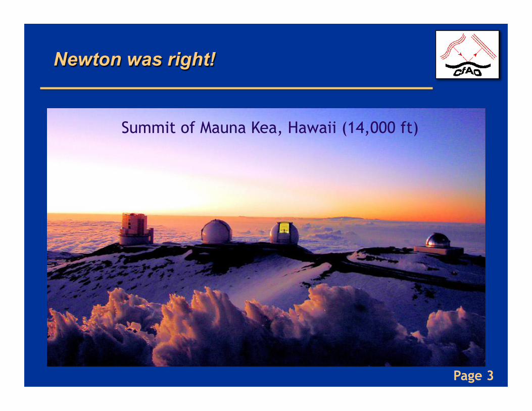
Newton was right!

Summit of Mauna Kea, Hawaii (14,000 ft)

Page 4

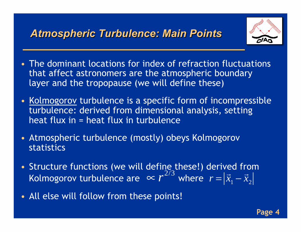
Atmospheric Turbulence: Main Points

•  The dominant locations for index of refraction fluctuations that affect astronomers are the atmospheric boundary layer and the tropopause (we will define these)

•  Kolmogorov turbulence is a specific form of incompressible turbulence: derived from dimensional analysis, setting heat flux in = heat flux in turbulence

•  Atmospheric turbulence (mostly) obeys Kolmogorov statistics

•  Structure functions (we will define these!) derived from Kolmogorov turbulence are where

•  All else will follow from these points!

∝ r2/3 r =!x1 −!x2

Page 5

Atmospheric Turbulence Issues for AO

• What determines the index of refraction in air?

• Origins of turbulence in Earth’s atmosphere

• Energy sources for turbulence

• Kolmogorov turbulence models

Page 6

Outline of lecture

• Physics of turbulence in the Earth’s atmosphere

–  Location

–  Origin

–  Energy sources

• Mathematical description of turbulence

– Goal: build up to derive an expression for r0, based on statistics of Kolmogorov turbulence

Page 7

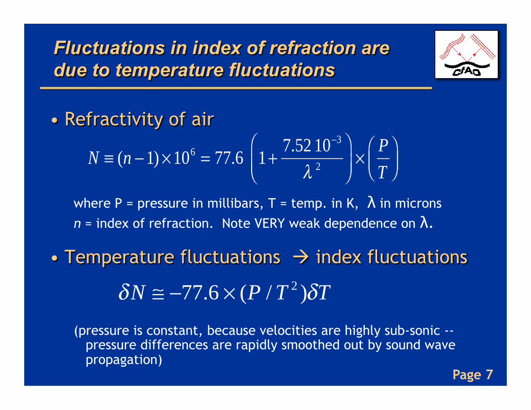
Fluctuations in index of refraction are due to temperature fluctuations

• Refractivity of air

where P = pressure in millibars, T = temp. in K, λ in microns n = index of refraction. Note VERY weak dependence on λ.

• Temperature fluctuations à index fluctuations

(pressure is constant, because velocities are highly sub-sonic --

pressure differences are rapidly smoothed out by sound wave propagation)

N ≡ (n −1) ×106 = 77.6 1+ 7.52 10−3

λ 2

⎛⎝⎜

⎞⎠⎟×

PT

⎛⎝⎜

⎞⎠⎟

δN ≅ −77.6 × (P / T 2 )δT

Page 8

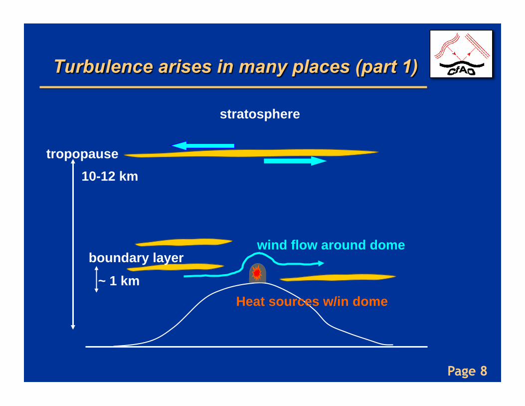
Turbulence arises in many places (part 1)

stratosphere!

Heat sources w/in dome"

boundary layer!~ 1 km"

tropopause!10-12 km"

wind flow around dome!

Page 9

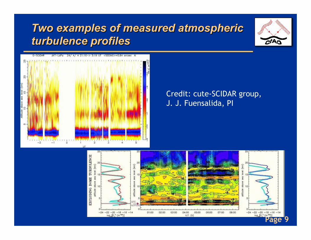
Two examples of measured atmospheric turbulence profiles

Credit: cute-SCIDAR group, J. J. Fuensalida, PI

Page 10

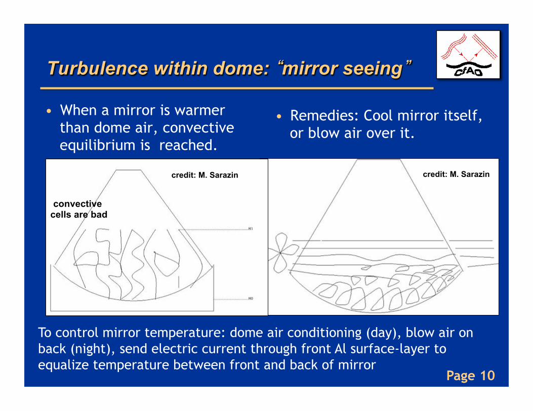
Turbulence within dome: “mirror seeing”

•  When a mirror is warmer than dome air, convective equilibrium is reached.

•  Remedies: Cool mirror itself, or blow air over it.

To control mirror temperature: dome air conditioning (day), blow air on back (night), send electric current through front Al surface-layer to equalize temperature between front and back of mirror

credit: M. Sarazin credit: M. Sarazin

convective cells are bad

Page 11

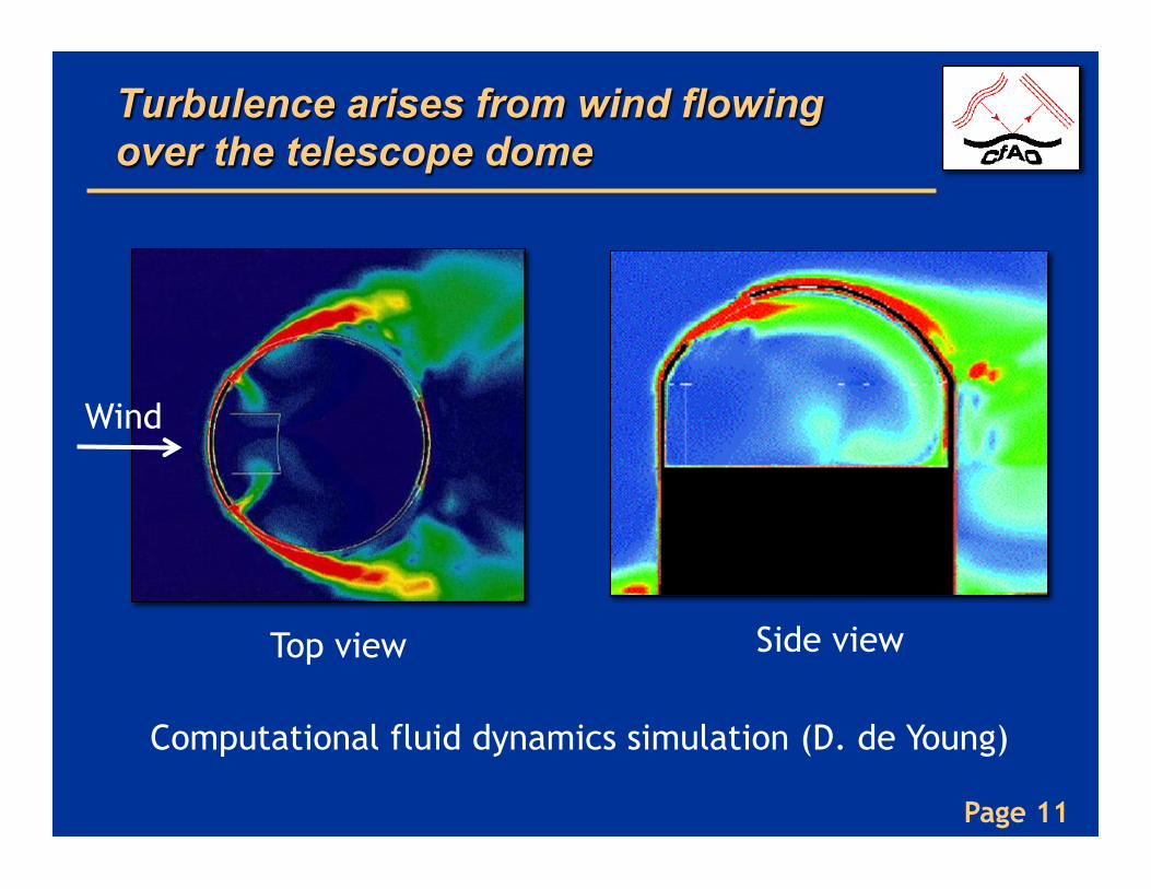
Turbulence arises from wind flowing over the telescope dome

Computational fluid dynamics simulation (D. de Young)

Top view Side view

Wind

Page 12

Turbulent boundary layer has largest effect on “seeing”

•  Wind speed must be zero at ground, must equal vwind several hundred meters up (in the “free atmosphere”)

•  Adjustment takes place at bottom of boundary layer –  Where atmosphere feels strong influence of earth’s surface –  Turbulent viscosity slows wind speed to zero at ground

•  Quite different between day and night –  Daytime: boundary layer is thick (up to a km), dominated by

convective plumes rising from hot ground. Quite turbulent. –  Night-time: boundary layer collapses to a few hundred

meters, is stably stratified. See a few “gravity waves.” Perturbed if winds are high.

Page 13

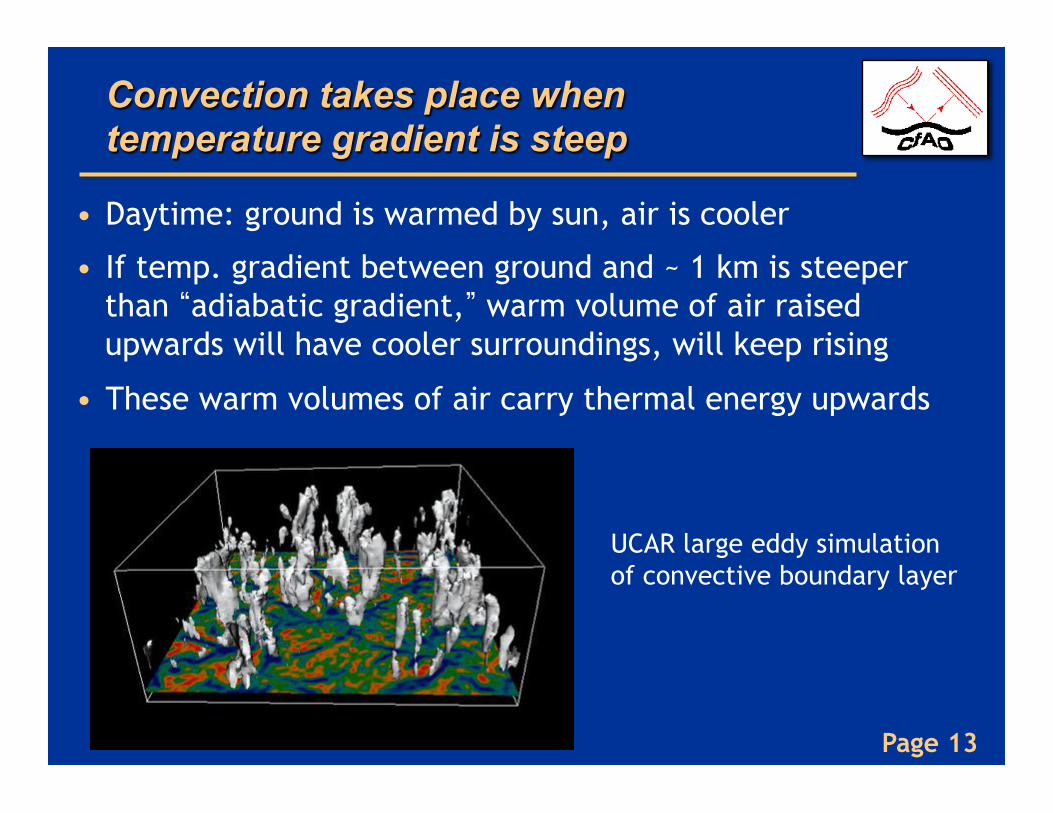
Convection takes place when temperature gradient is steep

•  Daytime: ground is warmed by sun, air is cooler

•  If temp. gradient between ground and ~ 1 km is steeper than “adiabatic gradient,” warm volume of air raised upwards will have cooler surroundings, will keep rising

•  These warm volumes of air carry thermal energy upwards

UCAR large eddy simulation of convective boundary layer

Page 14

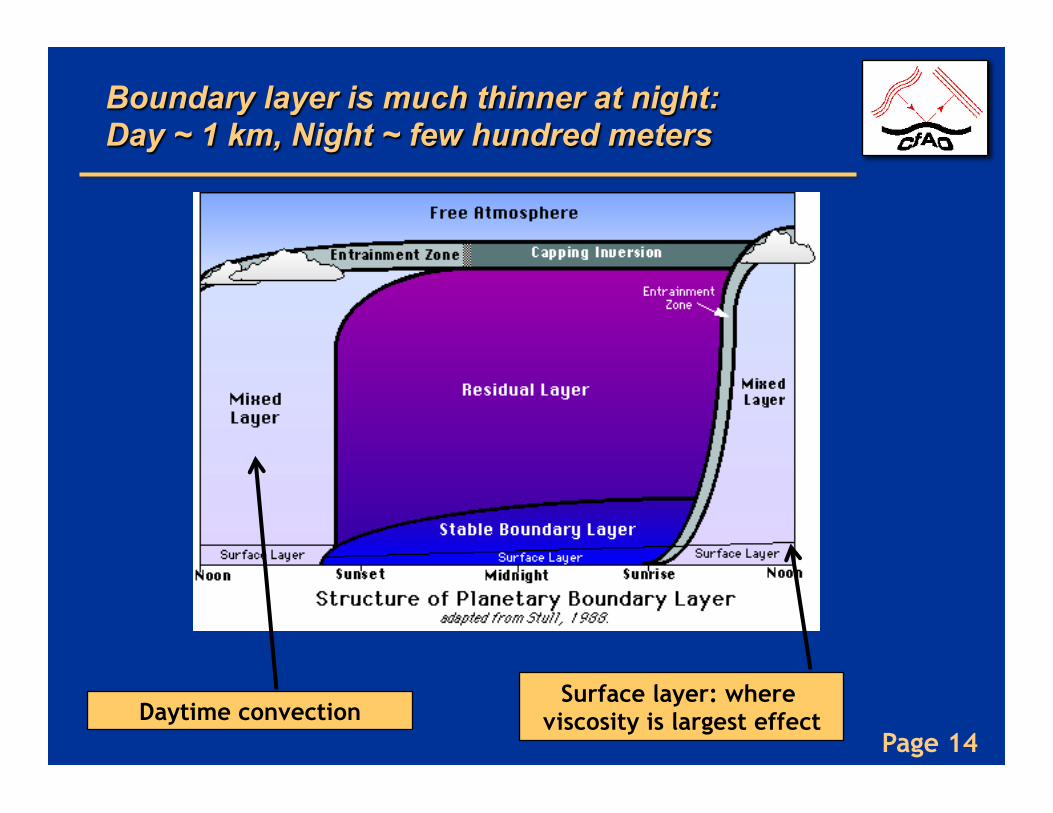
Boundary layer is much thinner at night: Day ~ 1 km, Night ~ few hundred meters

Surface layer: where viscosity is largest effect Daytime convection

Page 15

Implications: solar astronomers vs. night-time astronomers

• Daytime: Solar astronomers have to work with thick and messy turbulent boundary layer

• Night-time: Less total turbulence, but boundary layer is still single largest contribution to “seeing”

• Neutral times: near dawn and dusk – Smallest temperature difference between

ground and air, so wind shear causes smaller temperature fluctuations

Page 16

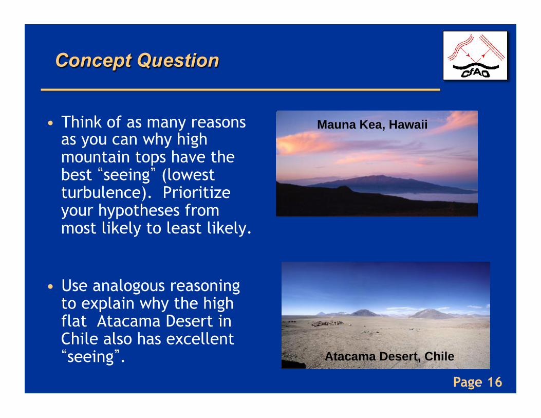
Concept Question

•  Think of as many reasons as you can why high mountain tops have the best “seeing” (lowest turbulence). Prioritize your hypotheses from most likely to least likely.

•  Use analogous reasoning to explain why the high flat Atacama Desert in Chile also has excellent “seeing”.

Mauna Kea, Hawaii

Atacama Desert, Chile

Page 17

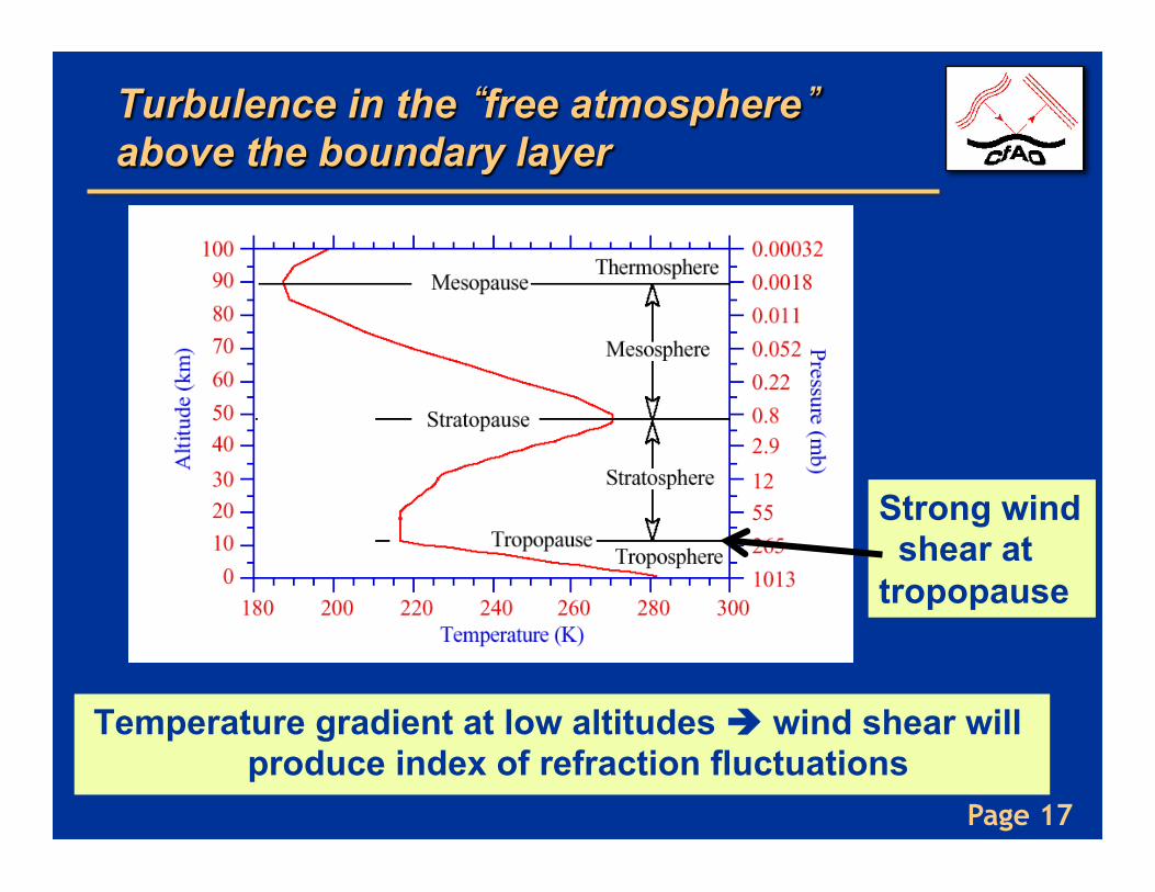
Strong wind shear at tropopause

Turbulence in the “free atmosphere” above the boundary layer

Temperature gradient at low altitudes è wind shear will produce index of refraction fluctuations

Page 18

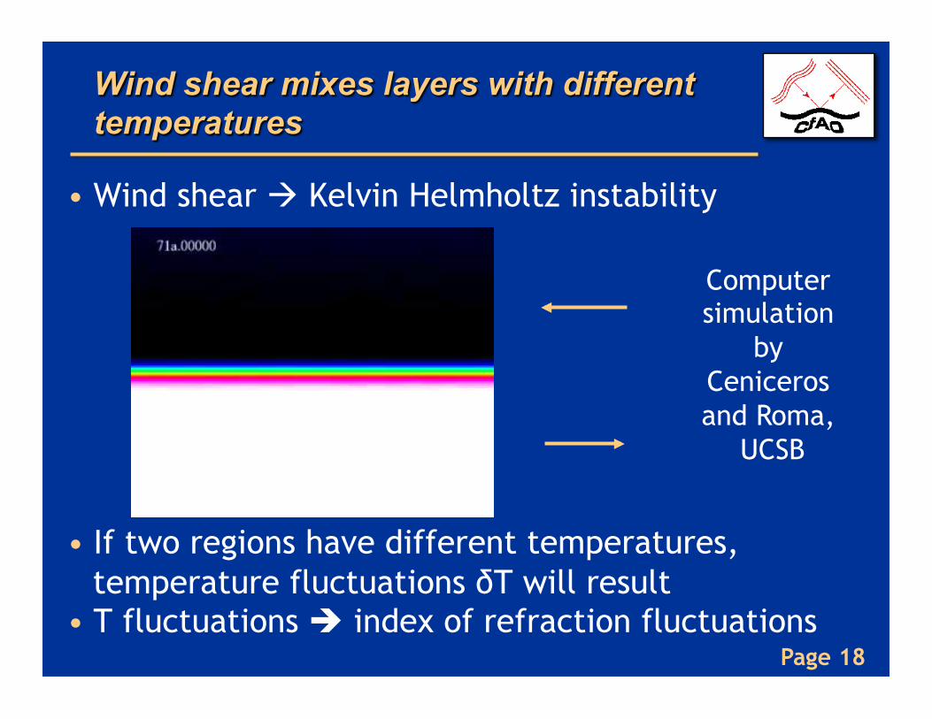
Wind shear mixes layers with different temperatures

• Wind shear à Kelvin Helmholtz instability

•  If two regions have different temperatures,

temperature fluctuations δT will result • T fluctuations è index of refraction fluctuations

Computer simulation

by Ceniceros and Roma,

UCSB

Page 19

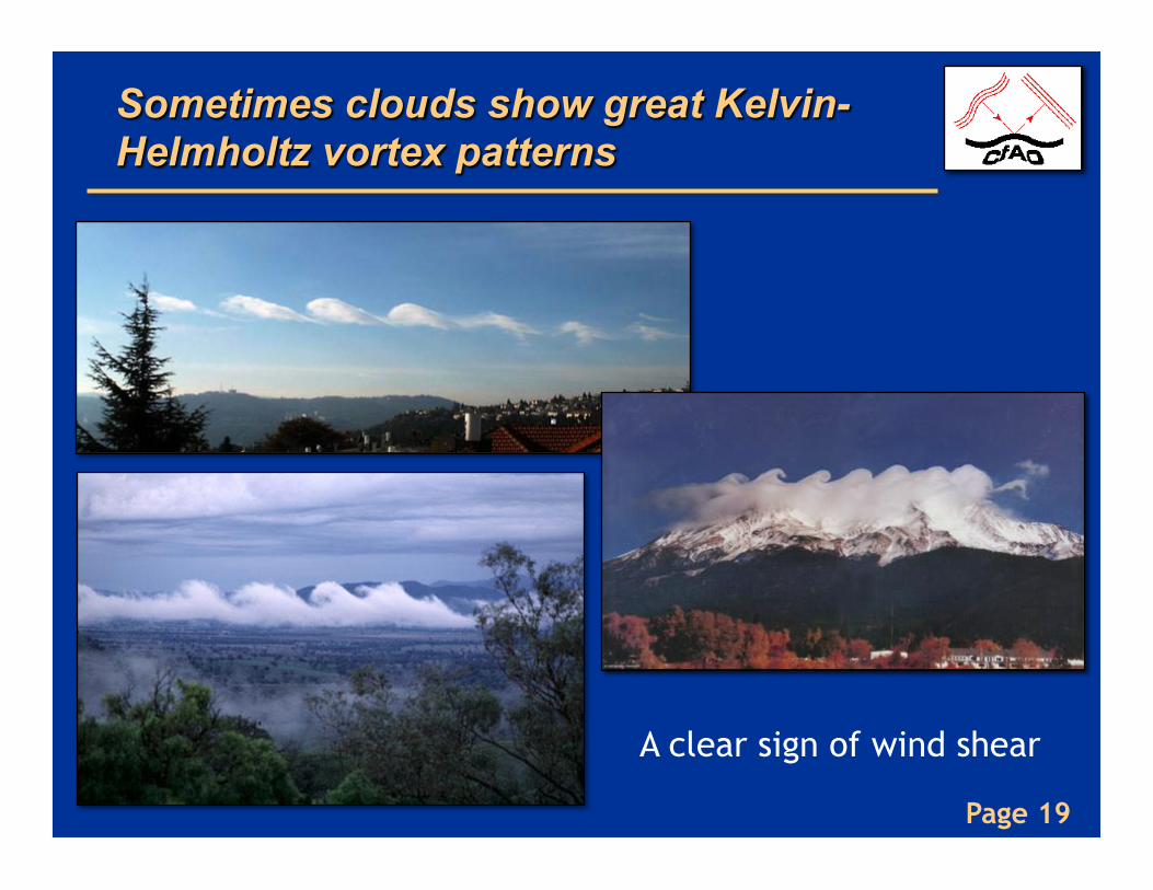
Sometimes clouds show great Kelvin-Helmholtz vortex patterns

A clear sign of wind shear

Page 20

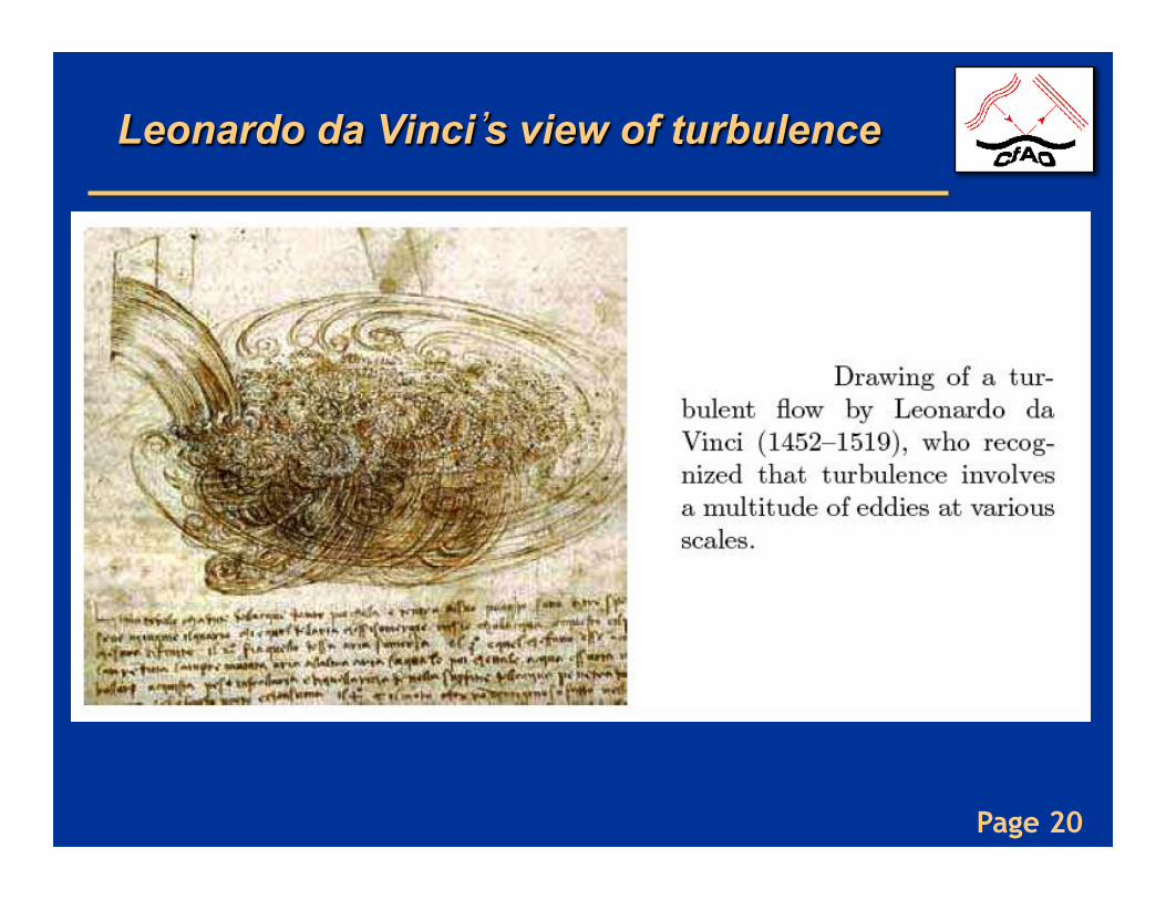
Leonardo da Vinci’s view of turbulence

Page 21

Kolmogorov turbulence in a nutshell

Big whorls have little whorls,

Which feed on their velocity;

Little whorls have smaller whorls,

And so on unto viscosity.

L. F. Richardson (1881-1953)

Page 22

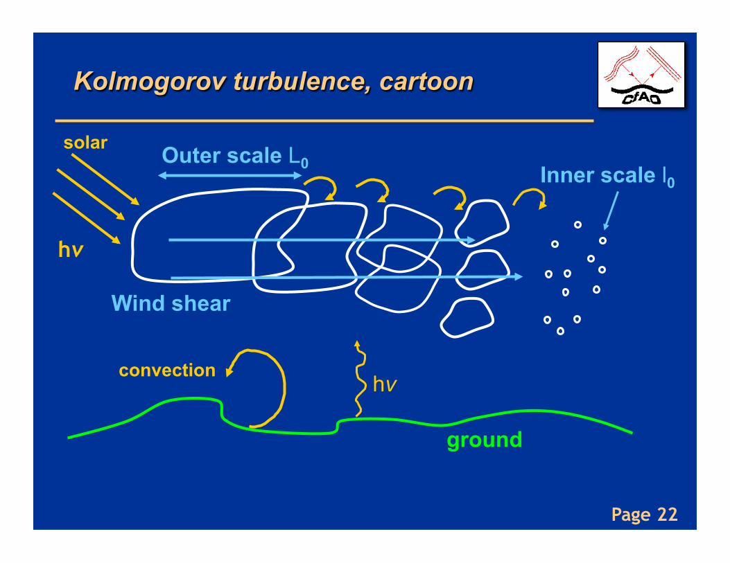
Kolmogorov turbulence, cartoon

Outer scale L0

ground

Inner scale l0

hν convection

solar

hν

Wind shear

Page 23

Kolmogorov turbulence, in words

•  Assume energy is added to system at largest scales - “outer scale” L0

•  Then energy cascades from larger to smaller scales (turbulent eddies “break down” into smaller and smaller structures).

•  Size scales where this takes place: “Inertial range”.

•  Finally, eddy size becomes so small that it is subject to dissipation from viscosity. “Inner scale” l0

•  L0 ranges from 10’s to 100’s of meters; l0 is a few mm

Page 24

Breakup of Kelvin-Helmholtz vortex

•  Start with large coherent vortex structure, as is formed in K-H instability

•  Watch it develop smaller and smaller substructure

•  Analogous to Kolmogorov cascade from large eddies to small ones

•  http://www.youtube.com/watch?v=hUXVHJoXMmU

Page 25

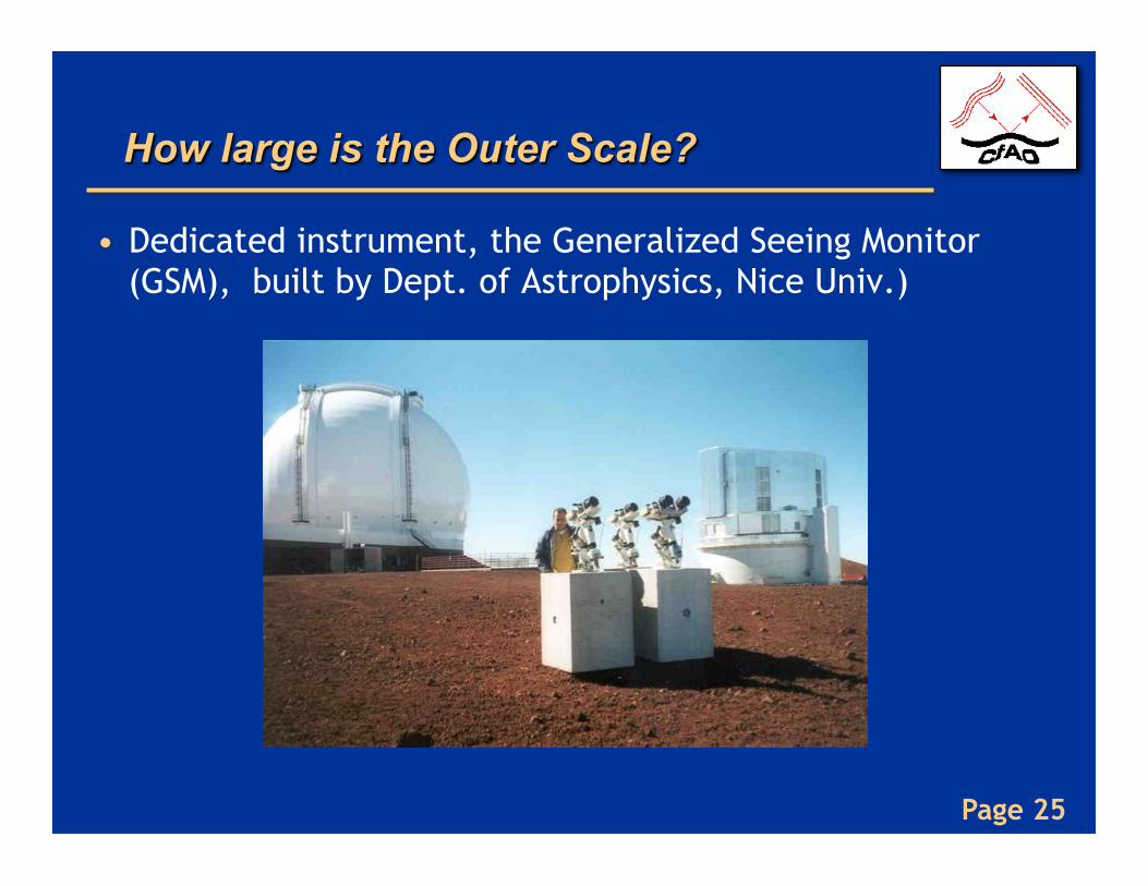
How large is the Outer Scale?

•  Dedicated instrument, the Generalized Seeing Monitor (GSM), built by Dept. of Astrophysics, Nice Univ.)

Page 26

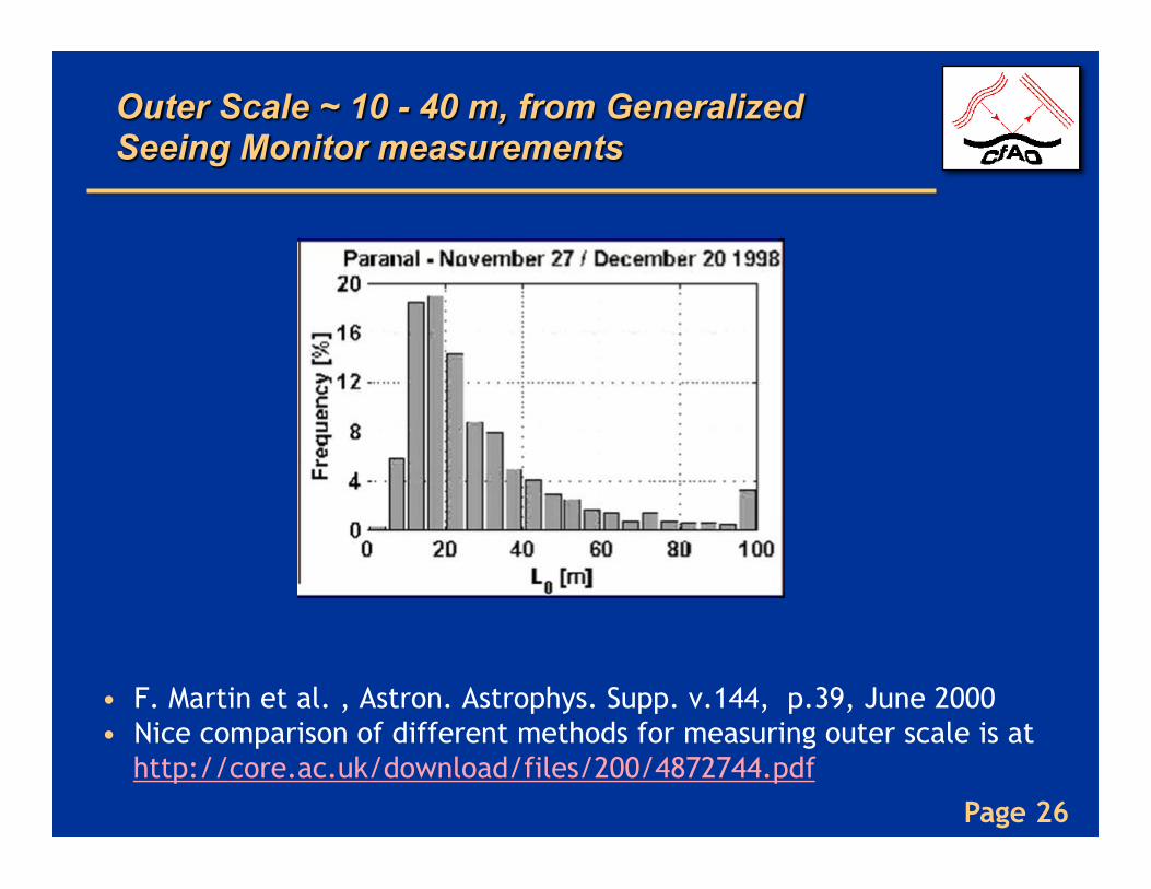
Outer Scale ~ 10 - 40 m, from Generalized Seeing Monitor measurements

•  F. Martin et al. , Astron. Astrophys. Supp. v.144, p.39, June 2000 •  Nice comparison of different methods for measuring outer scale is at

http://core.ac.uk/download/files/200/4872744.pdf

Page 27

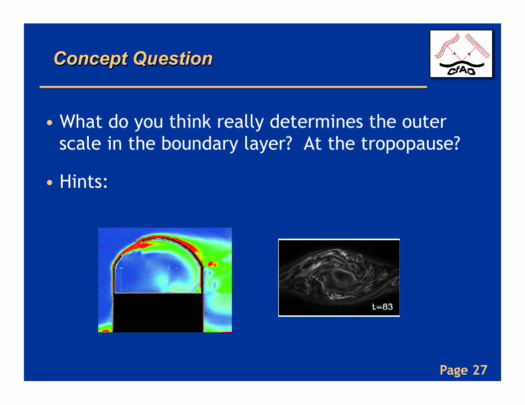
Concept Question

• What do you think really determines the outer scale in the boundary layer? At the tropopause?

• Hints:

Page 28

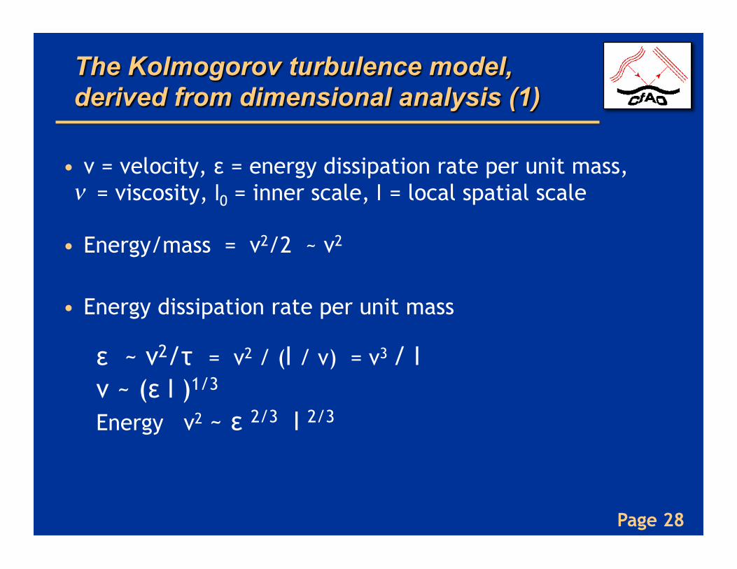
The Kolmogorov turbulence model, derived from dimensional analysis (1)

•  v = velocity, ε = energy dissipation rate per unit mass, = viscosity, l0 = inner scale, l = local spatial scale

•  Energy/mass = v2/2 ~ v2

•  Energy dissipation rate per unit mass

ε ~ v2/τ = v2 / (l / v) = v3 / l v ~ (ε l )1/3

Energy v2 ~ ε 2/3 l 2/3

ν

Page 29

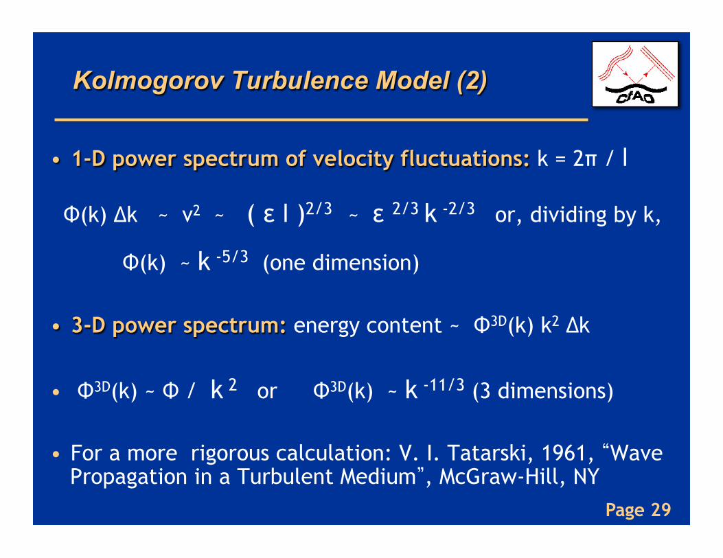
Kolmogorov Turbulence Model (2)

•  1-D power spectrum of velocity fluctuations: k = 2π / l

Φ(k) Δk ~ v2 ~ ( ε l )2/3 ~ ε 2/3 k -2/3 or, dividing by k,

Φ(k) ~ k -5/3 (one dimension)

•  3-D power spectrum: energy content ~ Φ3D(k) k2 Δk

•  Φ3D(k) ~ Φ / k 2 or Φ3D(k) ~ k -11/3 (3 dimensions)

•  For a more rigorous calculation: V. I. Tatarski, 1961, “Wave Propagation in a Turbulent Medium”, McGraw-Hill, NY

Page 30

k (cm-1)

Pow

er (

arbi

trar

y un

its)

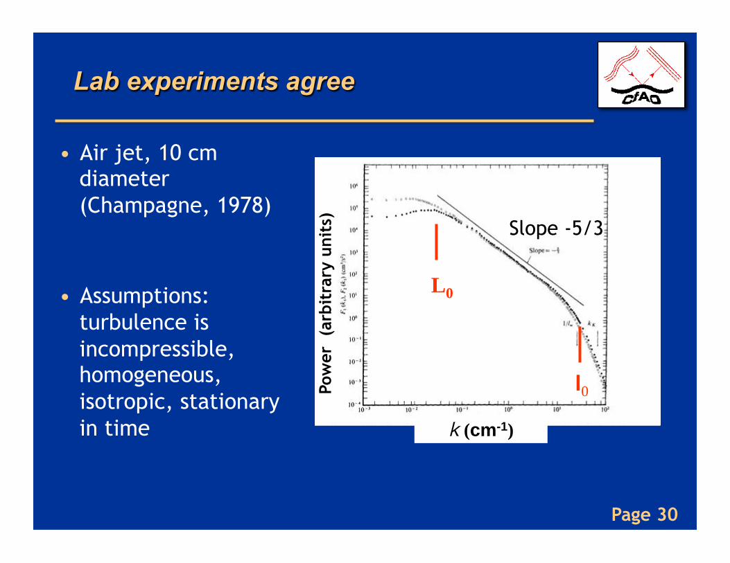
Lab experiments agree

•  Air jet, 10 cm diameter (Champagne, 1978)

•  Assumptions: turbulence is incompressible, homogeneous, isotropic, stationary in time

Slope -5/3

L0

l0

Page 31

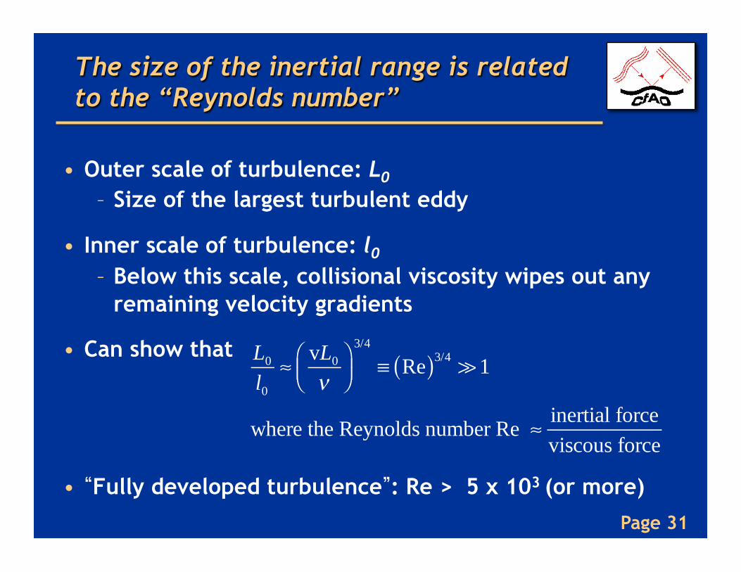
The size of the inertial range is related to the “Reynolds number”

•  Outer scale of turbulence: L0

–  Size of the largest turbulent eddy

•  Inner scale of turbulence: l0

–  Below this scale, collisional viscosity wipes out any remaining velocity gradients

•  Can show that

•  “Fully developed turbulence”: Re > 5 x 103 (or more)

L0

l0

≈ vL0

ν⎛⎝⎜

⎞⎠⎟

3/4

≡ Re( )3/4 1

where the Reynolds number Re ≈ inertial forceviscous force

Page 32

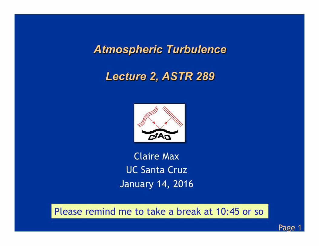
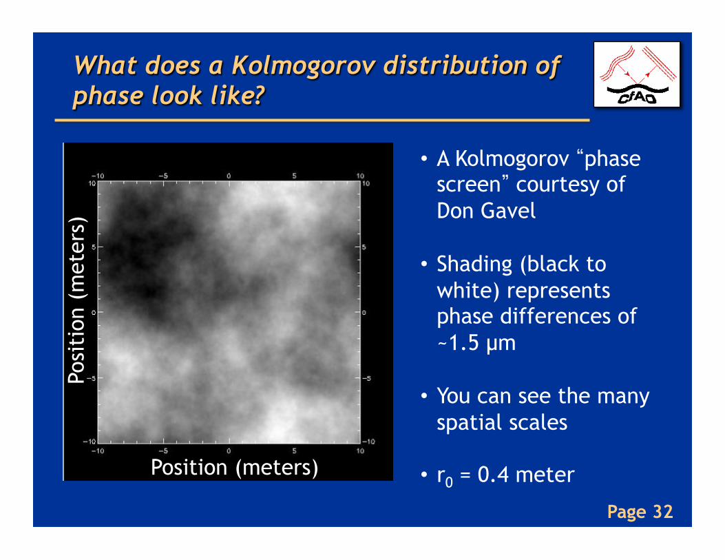
What does a Kolmogorov distribution of phase look like?

Position (meters)

Posi

tion

(m

eter

s)

•  A Kolmogorov “phase screen” courtesy of Don Gavel

•  Shading (black to white) represents phase differences of ~1.5 µm

•  You can see the many spatial scales

•  r0 = 0.4 meter

Page 33

Structure functions are used a lot in AO discussions. What are they?

•  Mean values of meteorological variables change with time over minutes to hours. Examples: T, p, humidity

•  If f(t) is a non-stationary random variable,

Ft(τ) = f ( t +τ) - f ( t) is a difference function that is stationary for small τ , varies for long τ.

•  Structure function is measure of intensity of fluctuations of f (t) over a time scale less than or equal to τ :

Df(τ) = < [ Ft(τ) ]2> = < [ f (t + τ) - f ( t) ]2 >

•  mean square

Page 34

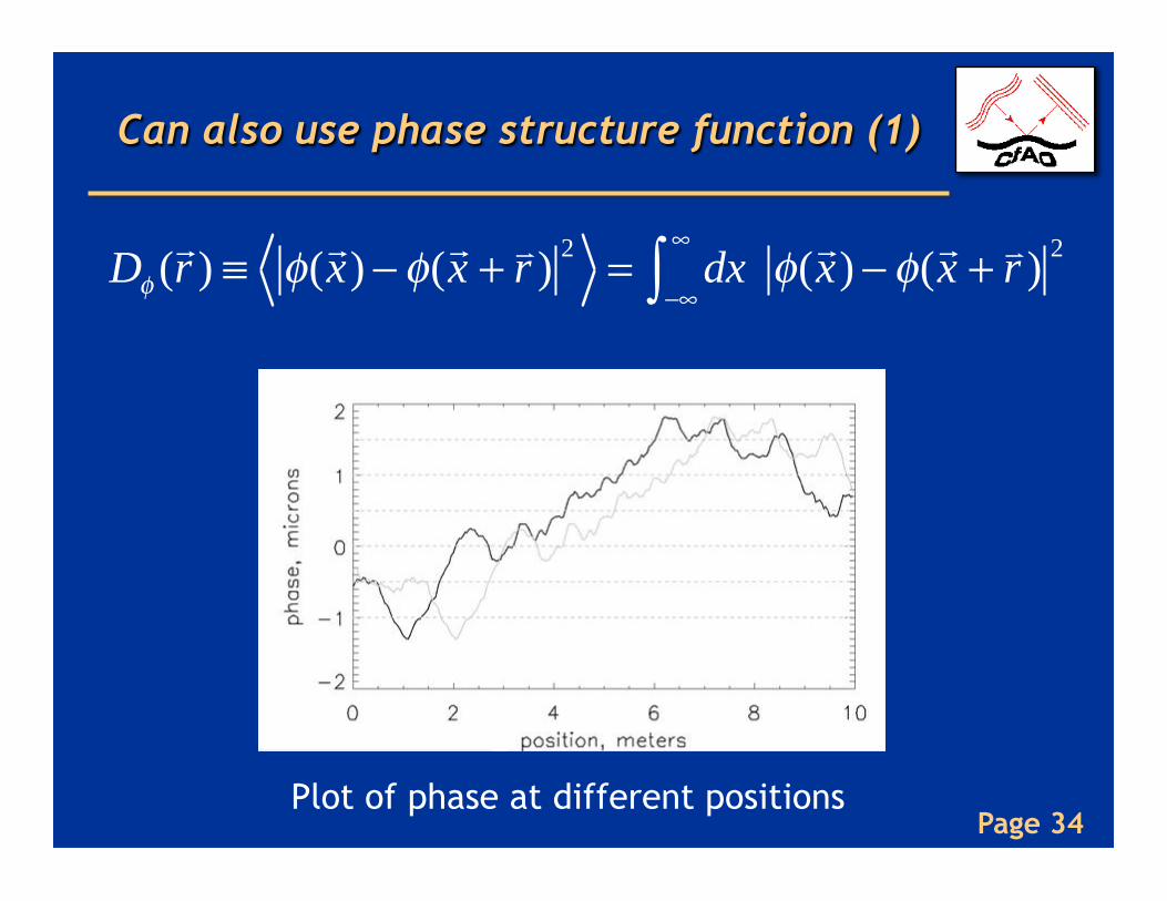
Can also use phase structure function (1)

Dφ (r ) ≡ φ(x) −φ(x + r ) 2 = dx

−∞

∞

∫ φ(x) −φ(x + r ) 2

Plot of phase at different positions

Page 35

Sidebar: different units to express phase

•  Φ Phase expressed as an angle in radians

•  Φ = (k� x) - ωt for a traveling wave

•  Φ in units of length? Φ ~ k x, or Φ/k ~ x

•  Φ in units of wavelength? Φ ~ k x ~ 2π(x/λ) –  So when Φ ~ 2π, x ~ λ. “One wave” of phase.

Page 36

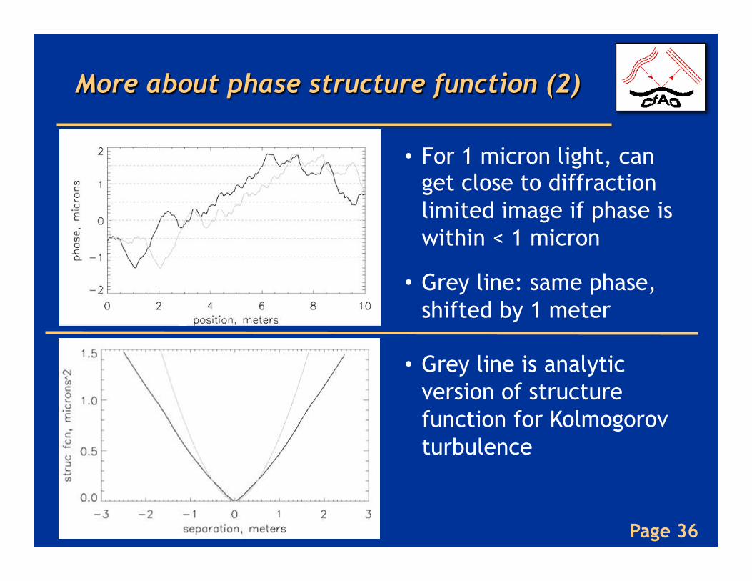
More about phase structure function (2)

•  For 1 micron light, can get close to diffraction limited image if phase is within < 1 micron

•  Grey line: same phase, shifted by 1 meter

•  Grey line is analytic

version of structure function for Kolmogorov turbulence

Page 37

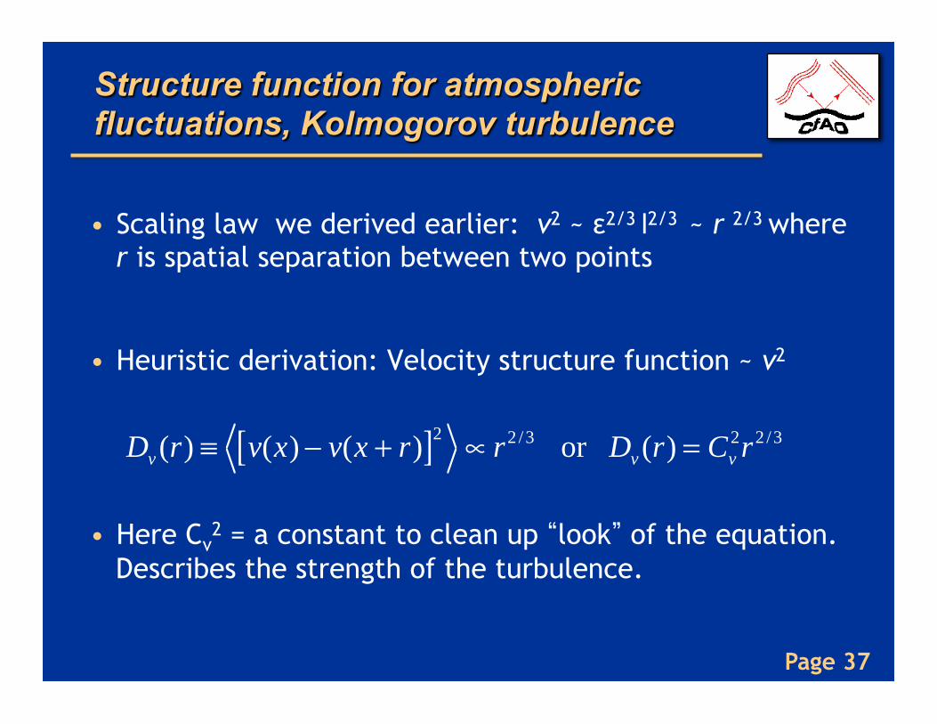
Structure function for atmospheric fluctuations, Kolmogorov turbulence

•  Scaling law we derived earlier: v2 ~ ε2/3 l2/3 ~ r 2/3 where r is spatial separation between two points

•  Heuristic derivation: Velocity structure function ~ v2

•  Here Cv2 = a constant to clean up “look” of the equation.

Describes the strength of the turbulence.

Dv (r) ≡ v(x) − v(x + r)[ ]2 ∝ r2 /3 or Dv (r) = Cv2r2 /3

Page 38

Derivation of Dv from dimensional analysis (1)

•  If turbulence is homogenous, isotropic, stationary

where f is a dimensionless function of a dimensionless argument.

• Dimensions of α are v2, dimensions of β are length, and they must depend only on ε and ν (the only free parameters in the problem).

[ ν ] ~ cm2 s-1 [ ε ] ~ erg s-1 gm-1 ~ cm2 s-3

Dv (x1, x2 ) = α × f (| x1 − x2 | /β)

Page 39

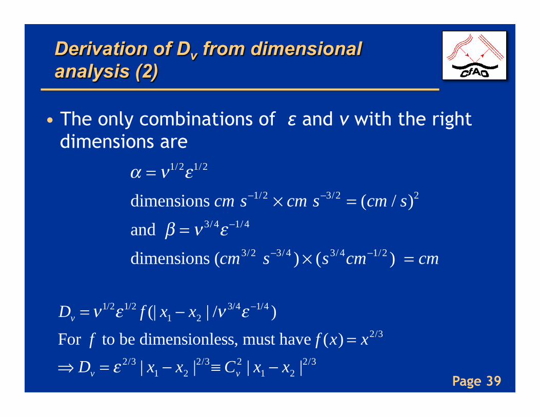
Derivation of Dv from dimensional analysis (2)

• The only combinations of ε and ν with the right dimensions are

α = ν1/2ε1/2

dimensions cm s−1/2 × cm s−3/2 = (cm / s)2

and β = ν 3/4ε−1/4

dimensions (cm3/2 s−3/4 ) × (s3/4cm−1/2 ) = cm

Dv = ν1/2ε1/2 f (| x1 − x2 | /ν 3/4ε −1/4 )

For f to be dimensionless, must have f (x) = x2/3

⇒ Dv = ε 2/3 | x1 − x2 |2/3≡ Cv2 | x1 − x2 |2/3

Page 40

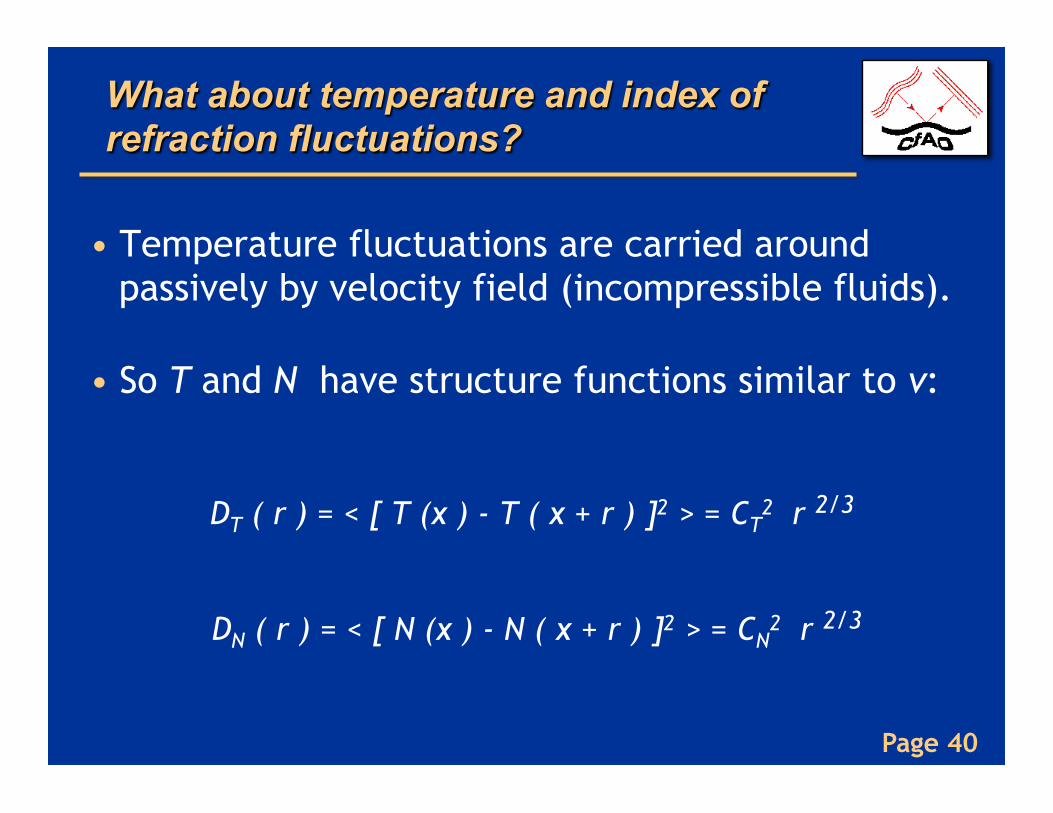
What about temperature and index of refraction fluctuations?

• Temperature fluctuations are carried around passively by velocity field (incompressible fluids).

• So T and N have structure functions similar to v:

DT ( r ) = < [ T (x ) - T ( x + r ) ]2 > = CT2 r 2/3

DN ( r ) = < [ N (x ) - N ( x + r ) ]2 > = CN2 r 2/3

Page 41

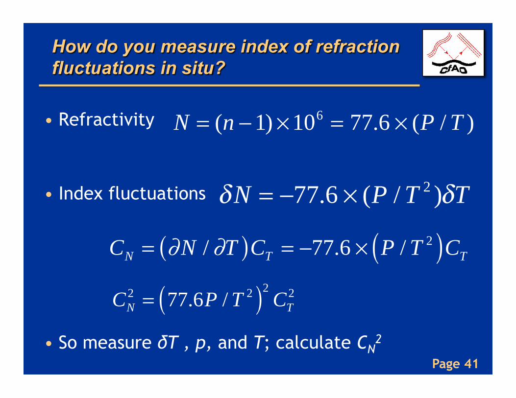
How do you measure index of refraction fluctuations in situ?

• Refractivity

•  Index fluctuations

• So measure δT , p, and T; calculate CN2

N = (n −1) ×106 = 77.6 × (P / T )

δN = −77.6 × (P / T 2 )δT

CN = ∂N / ∂T( )CT = −77.6 × P / T 2( )CT

CN2 = 77.6P / T 2( )2

CT2

Page 42

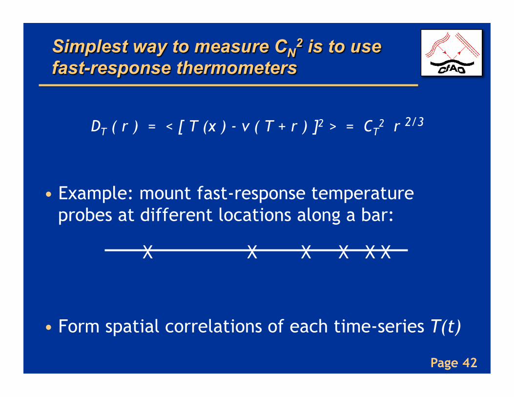
Simplest way to measure CN2 is to use

fast-response thermometers

DT ( r ) = < [ T (x ) - v ( T + r ) ]2 > = CT2 r 2/3

• Example: mount fast-response temperature probes at different locations along a bar:

X X X X X X

• Form spatial correlations of each time-series T(t)

Page 43

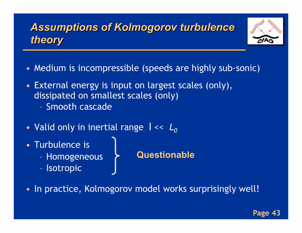
Assumptions of Kolmogorov turbulence theory

•  Medium is incompressible (speeds are highly sub-sonic)

•  External energy is input on largest scales (only), dissipated on smallest scales (only) –  Smooth cascade

•  Valid only in inertial range l << L0

•  Turbulence is –  Homogeneous –  Isotropic

•  In practice, Kolmogorov model works surprisingly well!

Questionable

Page 44

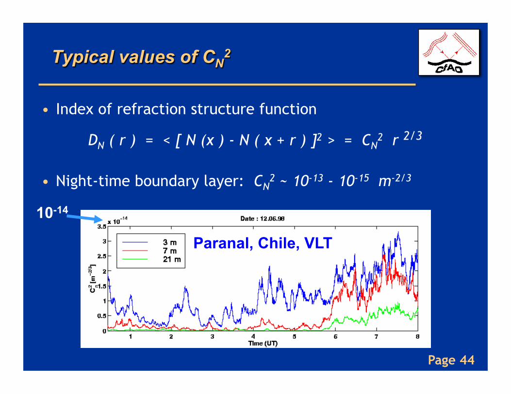
Typical values of CN2

•  Index of refraction structure function

DN ( r ) = < [ N (x ) - N ( x + r ) ]2 > = CN2 r 2/3

•  Night-time boundary layer: CN2 ~ 10-13 - 10-15 m-2/3

10-14

Paranal, Chile, VLT

Page 45

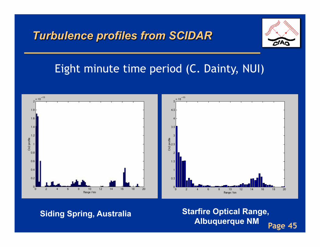
Turbulence profiles from SCIDAR

Eight minute time period (C. Dainty, NUI)

Siding Spring, Australia Starfire Optical Range, Albuquerque NM

Page 46

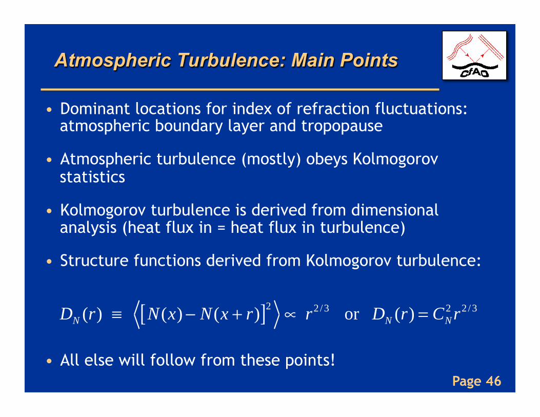
Atmospheric Turbulence: Main Points

•  Dominant locations for index of refraction fluctuations: atmospheric boundary layer and tropopause

•  Atmospheric turbulence (mostly) obeys Kolmogorov statistics

•  Kolmogorov turbulence is derived from dimensional analysis (heat flux in = heat flux in turbulence)

•  Structure functions derived from Kolmogorov turbulence:

•  All else will follow from these points!

DN (r) ≡ N(x) − N(x + r)[ ]2 ∝ r2 /3 or DN (r) = CN2 r2 /3

Page 47

Part 2: Effect of turbulence on spatial coherence function of light

• We will use structure functions D ~ r2/3 to calculate various statistical properties of light propagation thru index of refraction variations

• I will outline calculation in class. Reading in Section 4: Quirrenbach goes into gory detail. I will ask you to write down the full analysis in your homework.

Page 48

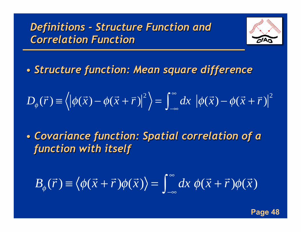
Definitions - Structure Function and Correlation Function

• Structure function: Mean square difference

• Covariance function: Spatial correlation of a function with itself

Dφ (r ) ≡ φ(x) −φ(x + r ) 2 = dx

−∞

∞

∫ φ(x) −φ(x + r ) 2

Bφ (r ) ≡ φ(x + r )φ(x) = dx

−∞

∞

∫ φ(x + r )φ(x)

Page 49

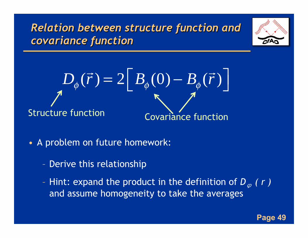
Relation between structure function and covariance function

•  A problem on future homework:

–  Derive this relationship

–  Hint: expand the product in the definition of Dϕ ( r ) and assume homogeneity to take the averages

Dφ (r ) = 2 Bφ (0) − Bφ (r )⎡⎣ ⎤⎦

Structure function Covariance function

Page 50

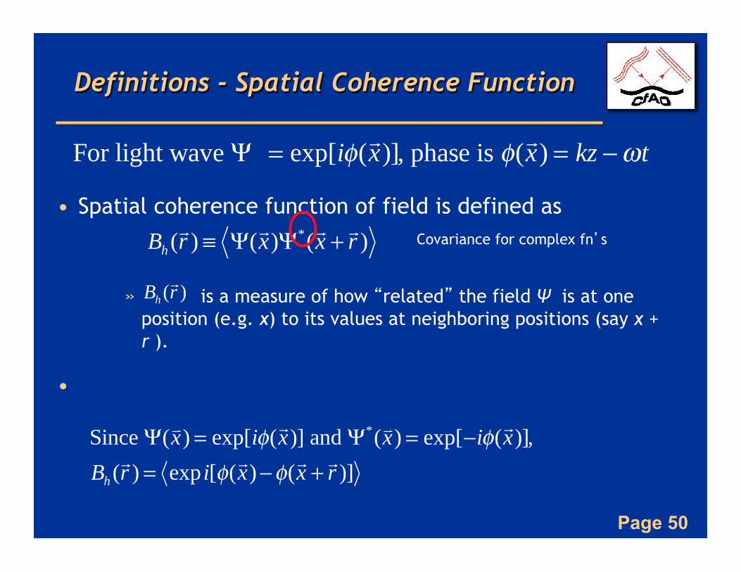
Definitions - Spatial Coherence Function

•  Spatial coherence function of field is defined as Covariance for complex fn’s

»  is a measure of how “related” the field Ψ is at one position (e.g. x) to its values at neighboring positions (say x + r ).

• 

For light wave Ψ = exp[iφ(x)], phase is φ(x) = kz −ωt

Bh (!r ) ≡ Ψ(!x)Ψ*(!x + !r )

Bh (r )

Since Ψ(!x) = exp[iφ("x)] and Ψ*(!x) = exp[−iφ("x)],Bh ("r ) = exp i[φ("x)−φ("x + "r )]

Page 51

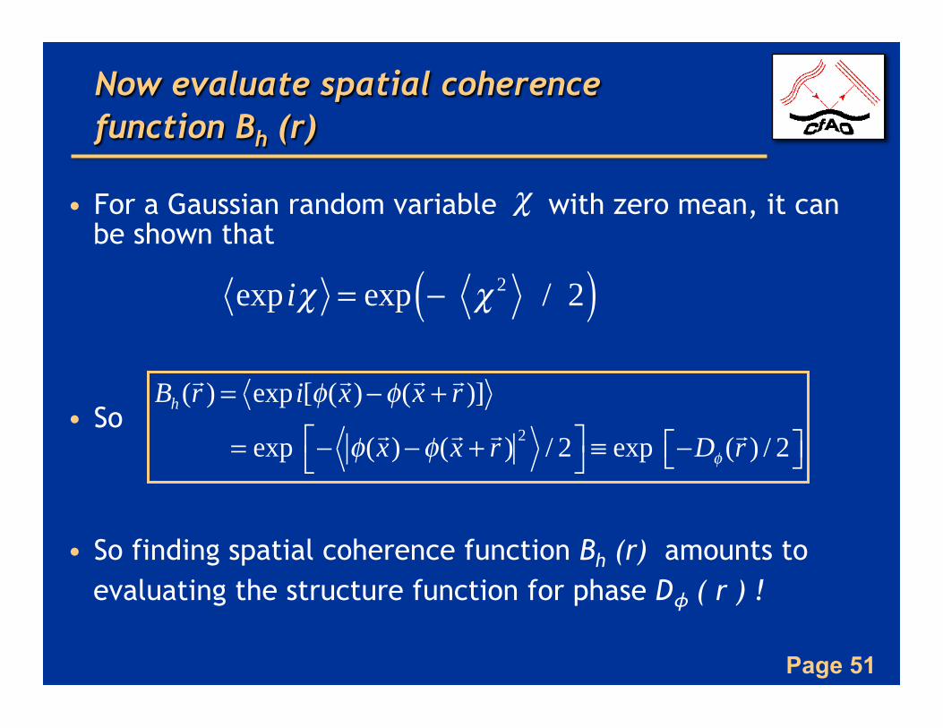
Now evaluate spatial coherence function Bh (r)

•  For a Gaussian random variable with zero mean, it can be shown that

•  So

•  So finding spatial coherence function Bh (r) amounts to evaluating the structure function for phase Dϕ ( r ) !

exp iχ = exp − χ 2 / 2( )

Bh (!r ) = exp i[φ(!x)−φ(!x + !r )]

= exp − φ(!x)−φ(!x + !r ) 2 / 2⎡⎣

⎤⎦ ≡ exp −Dφ (!r ) / 2⎡⎣ ⎤⎦

χ

Page 52

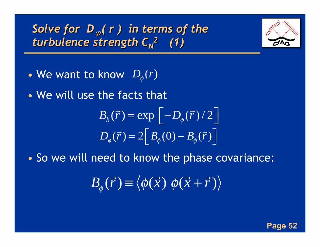
Solve for Dϕ( r ) in terms of the turbulence strength CN

2 (1)

• We want to know

• We will use the facts that

• So we will need to know the phase covariance: Dφ (r ) = 2 Bφ (0) − Bφ (r )⎡⎣ ⎤⎦ Bh (r ) = exp −Dφ (r ) / 2⎡⎣ ⎤⎦

Bφ (r ) ≡ φ(x) φ(x + r )

Dφ (r)

Page 53

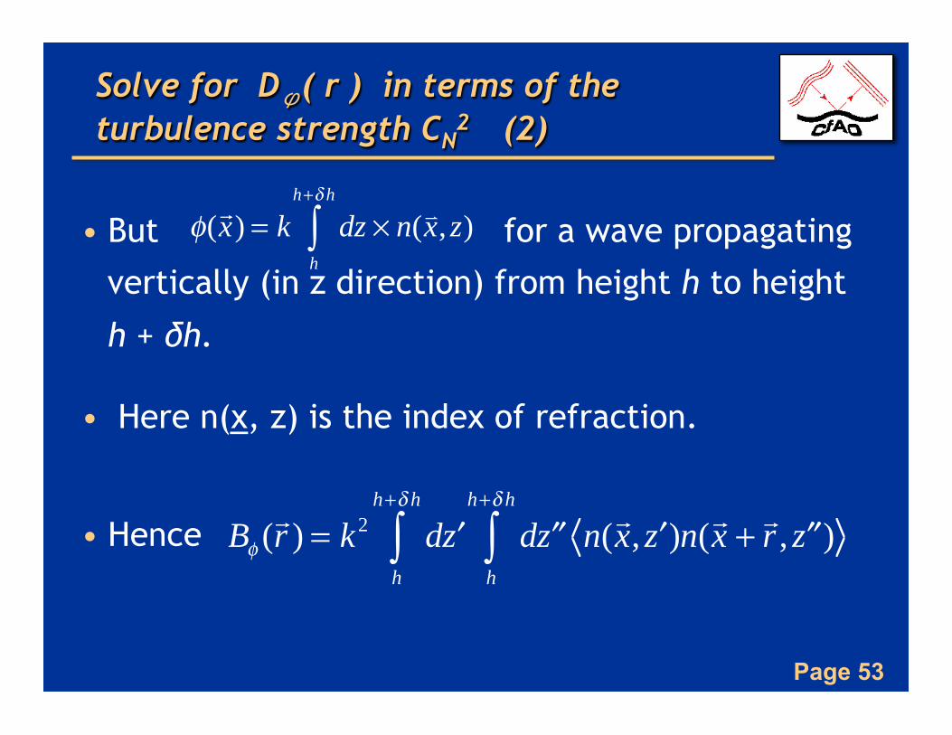
Solve for Dϕ( r ) in terms of the turbulence strength CN

2 (2)

• But for a wave propagating

vertically (in z direction) from height h to height

h + δh.

•  Here n(x, z) is the index of refraction.

• Hence Bφ (r ) = k2 d ′z

h

h+δ h

∫ d ′′zh

h+δ h

∫ n(x, ′z )n(x + r , ′′z )

φ(x) = k dz × n(x, z)

h

h+δ h

∫

Page 54

Solve for Dϕ( r ) in terms of the turbulence strength CN

2 (3)

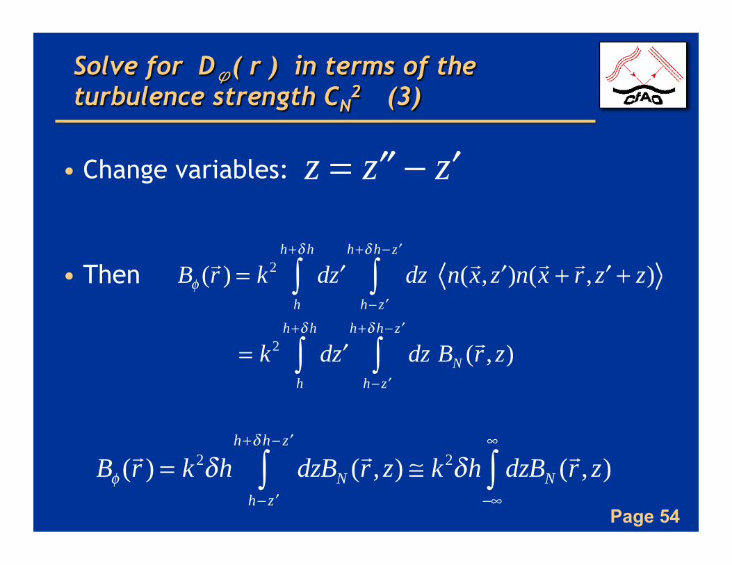
• Change variables:

• Then

z = ′′z − ′z

Bφ (r ) = k2 d ′zh

h+δ h

∫ dz n(x, ′z )n(x + r , ′z + z)h− ′z

h+δ h− ′z

∫

= k2 d ′zh

h+δ h

∫ dz BNh− ′z

h+δ h− ′z

∫ (r , z)

Bφ (r ) = k2δh dzBN

h− ′z

h+δ h− ′z

∫ (r , z) ≅ k2δh dzBN−∞

∞

∫ (r , z)

Page 55

Solve for Dϕ( r ) in terms of the turbulence strength CN

2 (4)

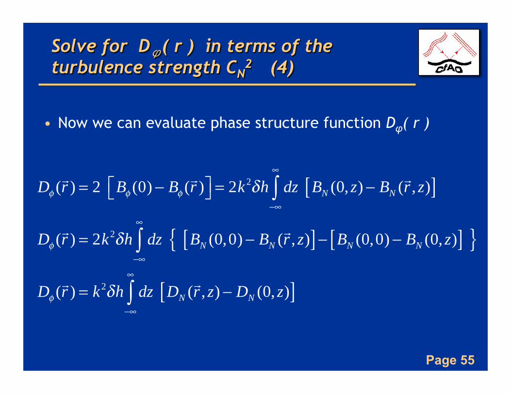
•  Now we can evaluate phase structure function Dφ( r )

Dφ (r ) = 2 Bφ (0) − Bφ (r )⎡⎣ ⎤⎦ = 2k2δh dz BN (0, z) − BN (r , z)[ ]−∞

∞

∫

Dφ (r ) = 2k2δh dz BN (0,0) − BN (r , z)[ ]− BN (0,0) − BN (0, z)[ ] { }−∞

∞

∫

Dφ (r ) = k2δh dz−∞

∞

∫ DN (r , z) − DN (0, z)[ ]

Page 56

Solve for Dϕ( r ) in terms of the turbulence strength CN

2 (5)

• 

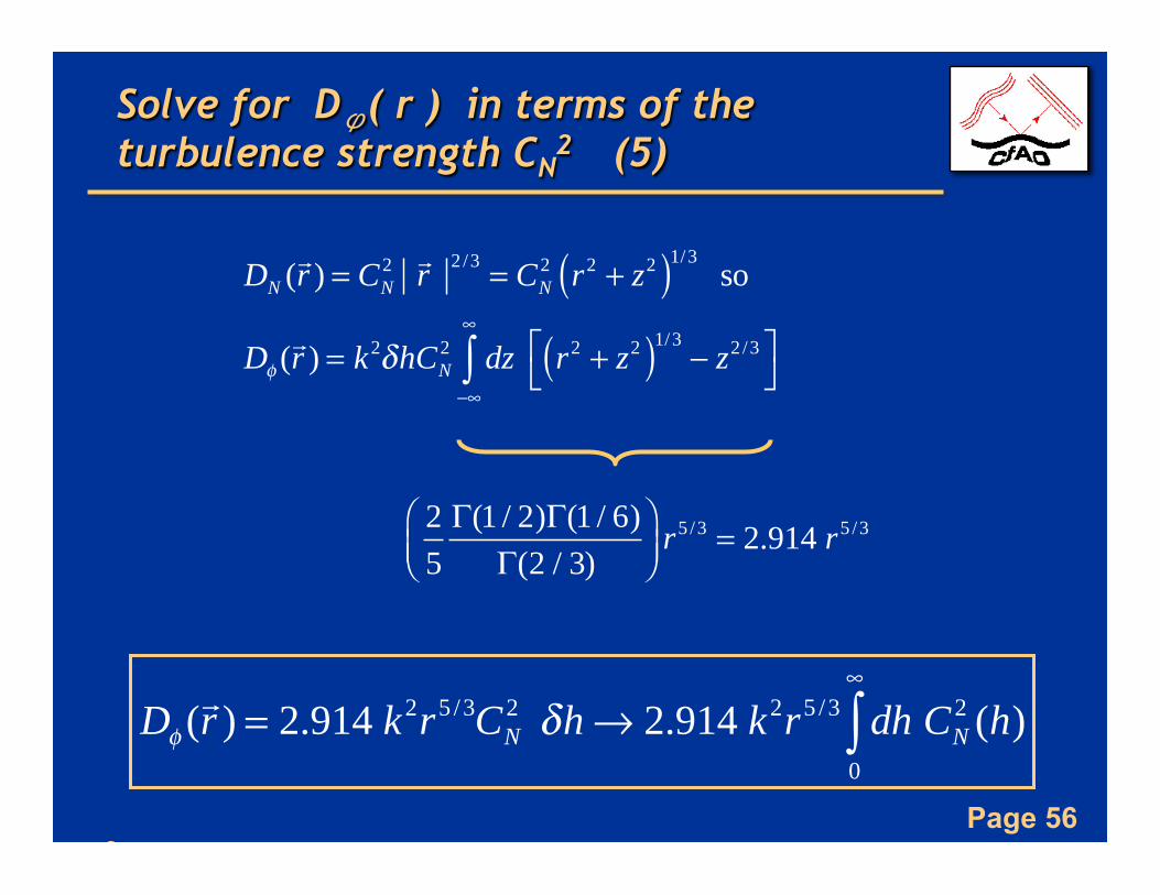
25Γ(1 / 2)Γ(1 / 6)

Γ(2 / 3)⎛⎝⎜

⎞⎠⎟

r5 /3 = 2.914 r5 /3

DN (r ) = CN2 r 2 /3 = CN

2 r2 + z2( )1/3 so

Dφ (r ) = k2δhCN2 dz r2 + z2( )1/3

− z2 /3⎡⎣

⎤⎦

−∞

∞

∫

Dφ (r ) = 2.914 k2r5 /3CN

2 δh → 2.914 k2r5 /3 dh 0

∞

∫ CN2 (h)

Page 57

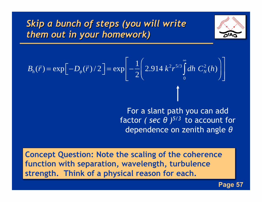
Skip a bunch of steps (you will write them out in your homework)

For a slant path you can add factor ( sec θ )5/3 to account for

dependence on zenith angle θ

Concept Question: Note the scaling of the coherence function with separation, wavelength, turbulence strength. Think of a physical reason for each.

Bh (!r ) = exp −Dφ (!r ) / 2⎡⎣ ⎤⎦ = exp − 1

22.914 k2r5/3 dh CN

2 (h)0

∞

∫⎛⎝⎜

⎞⎠⎟

⎡

⎣⎢⎢

⎤

⎦⎥⎥

Page 58

Given the spatial coherence function, calculate effect on telescope resolution

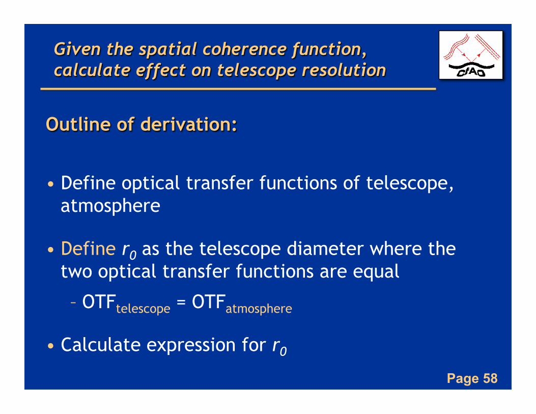
Outline of derivation:

• Define optical transfer functions of telescope, atmosphere

• Define r0 as the telescope diameter where the two optical transfer functions are equal

– OTFtelescope = OTFatmosphere

• Calculate expression for r0

Page 59

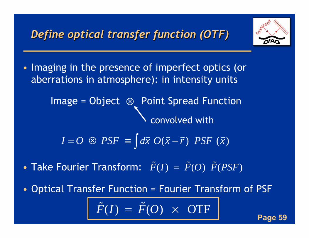
Define optical transfer function (OTF)

•  Imaging in the presence of imperfect optics (or aberrations in atmosphere): in intensity units

Image = Object Point Spread Function

•  Take Fourier Transform:

• Optical Transfer Function = Fourier Transform of PSF

convolved with

⊗

I = O ⊗ PSF ≡ dx O(x − r ) PSF (x)∫

F(I ) = F(O) F(PSF)

F(I ) = F(O) × OTF

Page 60

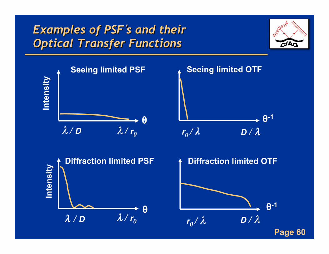
Examples of PSF’s and their Optical Transfer Functions

Seeing limited PSF

Diffraction limited PSF

Inte

nsity

θ

θ

Inte

nsity

Seeing limited OTF

Diffraction limited OTF

λ / r0

λ / r0λ / D

λ / D r0 / λ D / λ

r0 / λ D / λ

θ-1

θ-1

Page 61

Next time: Derive r0 and all the good things that come from knowing r0

• Define r0 as the telescope diameter where the optical transfer functions of the telescope and atmosphere are equal

• Use r0 to derive relevant timescales of turbulence

• Use r0 to derive “Isoplanatic Angle”: – AO performance degrades as astronomical

targets get farther from guide star