Embed Size (px)
Citation preview
Meteorological Training Course Lecture Series
ECMWF, 2002 1
Atmospheric waves
By Martin Miller
European Centre for Medium-Range Weather Forecasts
1. INTRODUCTION
In orderto understandthemany andvariedapproximationsandassumptionswhich aremadein designinga nu-
mericalmodelof theearthsatmosphere(whetherof small-scalefeaturessuchasindividual clouds,or mesoscale,
regional,globalweatherpredictionor climatemodels),it is necessaryto studythevariouswavemotionswhichcan
bepresent.Theidentificationandappreciationof themechanismsof thesewaveswill allow usto isolateor elim-
inatecertainwavetypesandto betterunderstandtheviability andeffectivenessof commonlymadeapproximations
such as assuming hydrostatic balance.
Herewewill attemptto identify thebasicatmosphericwavemotions,to emphasisetheirmostimportantproperties
andtheir physicalcharacteristics.Basictextbookssuchas'An Introductionto DynamicMeteorology'by Holton
or 'NumericalPredictionandDynamicMeteorology'by Haltiner and Williams provide a goodintroductionand
complementthis shortcoursewell. Whereasthesetextbookstreateachwavemotionseparatelystartingfrom dif-
ferentsimplifiedequationsets,we will separatewavesfrom a morecompleteequationsetby variousapproxima-
tionsmadeat laterstagesthusmakingit easierto relatetheimpactof a particularapproximationon severalwave
types. Nevertheless,to retainall wavetypesin theinitial equationsetis unmanageableandwewill introducesub-
sets of equations later.
We will restrictourselvesto neutral(non-amplifying,non-decaying)wavesin which energy exchangesareoscil-
latory.
While theexactequationshavebeenconsiderablysimplifiedinto ausefulform for studiesof atmosphericdynam-
ics,thesesimplifiedequationscannotbesolvedanalyticallyexceptin certainspecialcases.Themaindifficulty aris-
esthroughthenon-linearadvectiveterms , etc.Althoughthesetermscanconsiderablymodify the
linearsolutionsandarealsophysically significantbecausethey representtransferandfeedbackbetweendifferent
scalesof motion,thelinearizedequations(obtainedby removing second-orderadvectiveterms)areusefulfor iden-
tifying theorigin of distincttypesof wave(acoustic,gravity andcyclone)in theequations.It shouldbeunderstood
that althoughnonlinearitywill modify the acoustic,gravity andlong wavesit will not introduceany additional
wave types.Sincetheorigin of wavescanbeidentifiedin thelinearizedequationsandthesecanbesolvedanalyt-
ically, useful methods for filtering individual modes can be determined.
2. BASIC EQUATIONS
Thefollowing mathematicalanalysisrequiresa choiceof verticalcoordinate.While it is commonto usepressure
or a pressure-basedverticalcoordinatein large-scalemodelling,this is not a necessarytheoreticalrestrictionand
we can write the equations in (height), (pressure) or ( ), as follows:
-coordinates
v ∇⋅( )v v�
∇⋅
� � σ ���*⁄=
� ������, , ,( )

Atmospheric waves
2 Meteorological Training Course Lecture Series
ECMWF, 2002
(1)
(2)
(3)
(4)
(5)
where and
All source/sink terms are omitted.
-coordinates
An exact transformation of(1)–(5) to -coordinates gives:
(6)
(7)
(8)
(9)
(10)
where
(11)
and , , and
D D �-------- � �–
1ρ---∂�
∂�------–=
D �D �------- � +
1ρ---∂�
∂�------–=
D �D �--------- �+
1ρ---∂�
∂�------–=
∂ ∂�------
∂ �∂�------
∂ �∂�-------+ +
DD �------ ρln( )=
DD �------
�ln( ) κ D
D �------ �ln( )=
DD �------ ∂
∂ �----- ∂∂�------ � ∂
∂�------ � ∂∂�------+ + += κ
����-----=
� �������, , ,( )�
D D �-------- ���– 1 ε+( )∂Φ
∂�-------–=
D �D �------- ��+ 1 ε+( )∂Φ
∂�-------–=
����--------- 1 ε+( )∂Φ
∂�-------–=
∂ ∂�------
∂ �∂�------
∂ω∂�-------+ +
DD �------ 1 ε+( )ln{ }=
D�
D �--------- κω��------------=
ε 1�---
D �D �--------- 1
� 2------ D
D �------ DφD �-------= =
ω� �� �--------= Φ � �= D
D �------ ∂∂ �----- ∂
∂�------ � ∂∂�------ ω ∂
∂�------+ + +=

Atmospheric waves
Meteorological Training Course Lecture Series
ECMWF, 2002 3
-coordinates
Either by transforming(1)(5) or (6)–(11) we can obtain the exact -coordinate set:
(12)
(13)
(14)
(15)
(16)
where , and .
All partial derivatives respect their coordinate system.
Notethatputting in (3), and elsewheregivesthefamiliar large-scaleequationsets,but we
will not make this approximationat present.In principlethefollowing linearizedanalysiscanbedonein any co-
ordinate;we will useheightbut muchof this analysishasbeendonein pressureandsigmacoordinateselsewhere
(e.g.Kasahara, 1974;Miller, 1974;Miller and White, 1984).
For simplicity wewill supposethatthemotionis independentof andneglectthevariationof theCoriolisparam-
eterwith latitude( ). Also wewill considersmalldisturbancesonaninitially motionlessatmos-
phere. A non-zero basic flow and restoration of and non-zero will be considered later.
In orderto tracetheeffectof individual termswewill use‘tracerparameters' whichhave thevalue
1 but can be set to zero to eliminate the relevant term.
We define ,where and is a reference pressure (e.g. 105 Pa), and write
where denotesmallperturbationson a meanstateand definethe
basichorizontallystratifiedatmospherewith . Sinceweconsidersmallperturbationssuchthatprod-
ucts of perturbations can be negelcted and that , , we can write(1)–(5) as:
σ ��� σ, , ���*⁄ �,=( )
σ
D D �-------- � �– 1 ε+( )∂Φ
∂�-------–��� ∂
∂�------�
*ln( )–=
D �D �------- � + 1 ε+( )∂Φ
∂�-------–��� ∂
∂�------�
*ln( )–=
���σ
--------- 1 ε+( )∂Φ∂σ-------–=
∂ ∂�------
∂ �∂�------
∂σ̇∂σ------+ +
DD �------ �
*ln( ) DD �------+– 1 ε+( )ln{ }=
D�
D �--------- κ� σ̇
σ---
DD �------ �
*ln( )+
=
σ̇�
σ� �--------= DD �------ ∂
∂ �----- ∂∂�------ � ∂
∂�------ σ̇ ∂∂σ------+ + +=
D � D �⁄ 0= ε 0=
�β ∂� ∂�⁄ 0= =
β ∂ ∂�⁄�
1�
2�
3�
4, , ,
Θ θln≡ θ� � 00�--------
κ
= �00
= 0 δ = δ +
� = � 0 δ � = δ �+
� = � 0 δ � = δ �+
ρ = ρ0�( ) δρ+
� = �0�( ) δ�+
Θ = Θ0�( ) δΘ+
δ , δ � , δ � , δρ, δ� , δΘ ρ0�( ) � 0
�( ) Θ0�( ),,
∂� 0
∂�--------- � ρ0–=
δ� /p0 1« δρ /ρ0 1« δΘ /Θ0 1«
Atmospheric waves
4 Meteorological Training Course Lecture Series
ECMWF, 2002
(17)
(18)
(19)
(20)
(21)
where and .
EXERCISE:
DeriveEq. (19)
Thecoefficients � ��� in (17)–(21)areindependentof and , sotheseequationsarelinearand,in an
unboundedregion,admitsolutionsof theseparableform where canbeacomplex func-
tion, and and arethe -wavenumberandthefrequency respectively. Complex valuesof would imply am-
plifying/decaying waves which are not considered here.
The full solutionis theappropriateFourier sumof termsof this form over all wavenumbers.Sincewe shall be
looking at individual waves we choose to discuss individual wave components rather than the Fourier sum.
Inserting , , andthecorrespondingexpressionsfor ,
, , and into (17)-(21),andnotingthattheoperators , canbereplacedby and , re-
spectively, yields the following set of ordinary differential equations in the unknowns :
(22)
(23)
(24)
(25)
(26)
Then(22) and(23) give:
∂δ ∂ �---------- � δ �–
∂∂�------
δ�ρ0------
+ 0=
∂δ �∂ �--------- � δ + 0=
�4∂δ �∂ �----------- ∂
∂�------δ�ρ0------
�3� δ�
ρ0------– � δΘ–+ 0=
�2
∂∂ �-----
δρρ0------
∂δ ∂�---------- ∂δ �
∂�-----------�
1δ ��0
--------------–+ + 0=
∂∂ �-----δΘ δ � �+ 0=
� ∂∂�------ θ0ln( )= 1�
0-------
∂∂�------ ρ0ln( )–=
� � � 1�
0⁄ � �� �( ) �! � σ �+( )( )exp
� σ � σ
δ ˆ �( ) �! � σ �+( )( )exp= δ � � ˆ �( ) �! � σ �+( )( )exp= δ �δ� δρ δΘ ∂ ∂�⁄ ∂ ∂ �⁄ �" � σ
ˆ � ˆ � ˆ � ˆ ρ0⁄ ρ̂ ρ0⁄ Θ̂, , , , ,
� σ ˆ �#� ˆ– �" � ˆρ0-----+ 0=
� σ � ˆ �# ˆ+ 0=
�4 � σ � ˆ �d
d � ˆρ0-----
�3�� ˆρ0-----– � Θ̂–+ 0=
�2 � σ ρ̂
ρ0----- �" # ˆ �d
d � ˆ�
1 � ˆ�0
-----------–+ + 0=
� σΘ̂ � ˆ �+ 0=

Meteorological Training Course Lecture Series
ECMWF, 2002 5
(27)
(28)
Eliminating between(25) and(27), and using (26) and the relation:
where is the Laplacian speed of sound, gives:
(29)
Using (30)
to eliminate from (24) yields:
(31)
In general , , arefunctionsof � so and areobtainedby simultaneoussolutionof thetwo first
orderequations(29)and(31)andthe , , , fieldsobtainedfrom (27), (28), (30)and(25), respectively.
However, for ourpresentpurposesit is sufficient to considerconstant(mean)valuesof , and whichare
related by . Then the differential equation for the height variation of is:
(32)
3. EXACT SOLUTIONS OF THE LINEARIZED EQUATIONS
The exact linearized equation for , obtained by setting in (32), is:
(33)
ˆ σ σ2 � 2–-----------------
� ˆρ0-----–=
� ˆ �$� σ2 � 2–-----------------
� ˆρ0-----–=
ˆ
δΘ̂ 1γ---� ˆ�
0------ ρ̂
ρ0-----–
1� 2----� ˆρ0----- ρ̂
ρ0-----–= =
� ��
0=
�dd � ˆ � � 2
�1�0
-------– � ˆ � σ
�2� 2
----- 2
σ2 � 2–-----------------–
� ˆ
ρ0-----+ + 0=
Θ̂ �"� ˆ �σ----=
Θ̂
� σ �dd � � 3–
� ˆρ0----- � � �
4σ2–( ) � ˆ+ 0=
� 1�
0⁄ � � � ˆ � ˆ ρ0⁄ ˆ � ˆ Θ̂ ρ̂ ρ0⁄
� 1�
0⁄ �� � � 2⁄+ 1
�0⁄= � ˆ
σ � 2
2
d
d � � 2�
3–( )�
1�0
-------–+ �dd
+ � � �4σ2–( ) 2
σ2 � 2–-----------------
�2� 2
-----–
– � � 3 � � 2
�1�0
-------–
� ˆ = 0
� ˆ �1
�2
�3
�4 1= = = =
σ � 2
2
d
d 1�0
------- �dd
– � � σ2–( ) 2
σ2 � 2–----------------- 1
� 2----–
�%� 1�
0-------–
–+ � ˆ 0=

Atmospheric waves
6 Meteorological Training Course Lecture Series
ECMWF, 2002
Onesolutionof (33) is , andthecorrespondingdynamicalstructurecanbedeterminedby setting in
(22)–(26)to give and . This is geostrophicmotionin the -directionandis also
exactly hydrostatic. More detail of this solution will be considered later.
If in (33) then:
(34)
Setting leads to the differential equation:
(35)
In general,if thewave motionis confinedbetweenphysicalboundaries,then(35) mustbesolvedwith respectto
boundaryconditions—thatis mustsatisfythe differentialequation(35) andthe prescribedvaluesof on
theseboundaries.It is reasonableto supposethatonly wavesof a certainfrequency andwavenumbercansatisfy
all these constraints. For such waves the permissible values of the (characteristic) function
are calledeigenvalues and the solutions corresponding to these eigenvalues are calledeigenfunctions.
For simplicity we shall supposethat thefluid is unbounded(theboundedproblemwith at
(say)canbeattemptedasanexercise)andin thiscaseit is readilyseenthat is asolutionto (35)provided
that:
(36)
This frequency or 'dispersion' relationship is of fourth order in:
(37)
and contains two pairs of waves moving in the and directions, with:
(38)
σ 0= σ 0=
ˆ � ˆ 0= = � ˆ �" &�⁄( ) � ˆ ρ0⁄( )= �
σ 0≠
� 2
2
d
d � ˆ 1�0
------- �dd � ˆ–
2 � � σ2–( )σ2 � 2–
------------------------------- σ2
� 2-----+
� ˆ+ 0=
� ˆ � *�( ) � 2
�0⁄( )exp=
� 2
2
d
d � * 2 � � σ2–( )σ2 � 2–
------------------------------- σ2
� 2----- 1
4�
02
-----------–+ � *+ 0=
� * � *
' σ � � � � � 0, , ,, ,( ) 2 � � σ2–( )σ2 � 2–
------------------------------- σ2
� 2----- 1
4�
02
-----------–+=
� * 0= � �2⁄±=
� * e(*),+∝
- 2 2 � � σ2–( )σ2 � 2–
------------------------------- σ2
� 2----- 1
4�
02
-----------–+=
σ
σ4 σ2 � 2 � 2 2 - 2 1
4�
02
-----------+ + +– � 2 2 � � � 2 - 2 1
4�
02
-----------+ ++ 0=
�+ �–
σg2 1
2--- � 2 � 2 2 - 2 1
4�
02
-----------+ + + 1 1
4� 2 2 � � � 2 - 2 1
4�
02
-----------+ +
� 2 � 2 2 - 2 1
4�
02
-----------+ + +
2-----------------------------------------------------------------------–
12---
–=

Atmospheric waves
Meteorological Training Course Lecture Series
ECMWF, 2002 7
(39)
Thefirst pair of rootsrepresentinertial–gravity wavesandthesecondpair representacousticwaves. This is not
obvious,especiallywith thedegreeof complicationrepresentedin thesetwo relationships,soit is usefulto look at
extreme cases (i.e. short/long waves) to clarify the above classification.
In suchdispersionrelationsa basicunshearedzonalflow ( ) canbeincludedby replacing by ( ), i.e.
Doppler shifted.
3.1 Gravity Waves
In thetroposphere,the inertial frequency is smallcomparedwith theBrunt–Väisäläfrequency (a global
averageof ). Moreover their magnitudestogetherwith thoseof and satisfythefollowing
inequalities:
(40)
Using relation(40) and consideringshort waves such that , then(38) reduces to:
(41)
This is thedispersionrelationfor shortinternalgravity waves(wavelength km say).Sincethewavesarerel-
atively short they are not modified significantly by rotation (no� in (41)).
(41) defines an upper limit to the frequency, i.e. for , with a period of about 10 minutes.
Since , thepropagationis primarily in thevertical , with propagationspeedsof approx-
imately 10m/s.
We can substitute back into(22)–(26) and obtain the ‘geometry'.
EXERCISE:
Showthat theseoscillationsaretransverse(particlepathsparallel to wavefronts).Derivefrom(41)a relationship
between group velocity and phase velocity and consider its geometric interpretation.
Gravity wavesactasa signalto thesurroundingfluid of localisedchangesin potentialtemperature.Shortgravity
waves are dispersive since their phase velocity is a function of and they radiate energy.
Internalgravity wavesareexcitedby local diabaticor mechanicalforcing. A particularlyinteresting,important,
andubiquitoustypeof gravity waveisgeneratedwhenthereisstablystratifiedflow overorography. Theseareknow
asleewaves, astationarywavepatternoveranddownstreamof theobstacle.Relativeto themeanwind thephase
σa2 1
2--- � 2 � 2 2 - 2 1
4�
02
-----------+ + + 1 1
4� 2 2 � � � 2 - 2 1
4�
02
-----------+ +
� 2 � 2 2 - 2 1
4�
02
-----------+ + +
2-----------------------------------------------------------------------–
12---
+=
σ σ .+
� � �� � �⁄ 10 2–∼ � �
0
�02 � 2
� 2------------- � 2
� �--------� � � 0
2
� 2---------------- 1« « «
2 � � � 2⁄( )»
σg2 � � 2
2 - 2 1 4�
02⁄+ +( )
-------------------------------------------------≅
50≤
σg2 � �∼ 2 - 2»
2 - 2» σ2 2⁄ σ2 - 2⁄«( )
σg � �=
σ ⁄
Atmospheric waves
8 Meteorological Training Course Lecture Series
ECMWF, 2002
linesslopeupstream;energy mustbepropagatedupwardhencethephasevelocitymusthaveadownwardcompo-
nent (this follows from the previous exercise). Since the waves are stationary :
.
This can be solved for (given ) to give the phaseslopes. For vertical propagation , i.e.
, hencefavourableleewaveconditionsrequiresuitablelocalcombinationsof mountain/hillgeometry
and large-scale flow.
Theimportanceof vertically propagatinggravity waves,especiallyleewaves,in forecastandclimatemodelshas
attractedrecentattentionandtheirassociatedverticalmomentumfluxesappearto beasignificantfactorin thedy-
namics of the large-scale circulation and of the stratosphere in particular.
As wemovetowardsthelongwave limit of (38) theinfluenceof rotation(through ) is increasinglyfelt andthese
long inertial gravity waveshave frequenciestendingtowards / Their horizontalphasespeedsbecomelarge,of
relevancein the designof time-integration schemesand in the problemof initialisation. The limiting caseof
represents a pureinertial wave with neither buoyancy or pressure forces important.
EXERCISE:
Substitute back into(22)–(26).
3.2 Acoustic waves
In asimilarmannerwecanexamine(39). Theinequalitiesin (40)areindependentof thecharacterof theoscillation
and consideringshort waves such that it follows that:
(42)
Also if , then:
(43)
The structure of these short waves may be found by substituting Eq.(43) back into(22)–(26).
EXERCISE:
Show that these waves are longitudinal with negligible temperature changes.
Themotiontransmitspressureperturbationswith a speedc, thespeedof sound,for all wavelengths—i.e.themo-
tion is nondispersive.
For long acoustic waves i.e. , and it is readily deduced that:
��0 0=
� � 2 - 2 1 4
�02⁄+ +( )
1 2⁄--------------------------------------------------------=
- 1 �, , - 2 0> � � ⁄<
��
σ �=
σ �=
2 � � � 2⁄»
σa2 � 2 2 - 2 1 4
�02⁄+ +( )≅
2 - 2 1 4�
02⁄+( )»
σa2 � 2 2≅
σ2 � 2» σ2 � �» 0→
Atmospheric waves
Meteorological Training Course Lecture Series
ECMWF, 2002 9
(44)
Since , arehorizontalandverticalphasespeeds,respectively, wecandeducethatshortacousticwaves
propagate with wave fronts almost vertical and vice-versa for long waves.
4. SIMPLIFIED SOLUTIONS TO THE LINEARIZED EQUATIONS—FILTERING APPROXIMA TIONS
It is usefulto simplify theexactlinearizedequationssincewecanthenextendthephysicalprinciplesbehindthese
approximations to simplify the much more complicated non-linear equations.
In particular, in thissectionweshallshow how soundwavesandgravity wavescanbefiltered,anddeterminecon-
ditions under which the static approximation to the pressure field is valid.
It is notobvious‘a priori' how anapproximationmadein oneequationfeedsthroughto affect termsin otherequa-
tionsandhencemodify themathematicalandphysicalsolutions.Wethereforecarryout thenecessaryelimination
rathercarefullyandfor this purposewe retaintheparameters to tracetheeffectsof anapproxima-
tion. However, we seefrom (32) that and occurin thecombination which vanishesin theexact
equations . Consequently, a spurioustermwill ariseif we neglect but retain , or
vice-versa.We thereforemusteitherretainboth and or neglectboth.We thereforehave to set in
(32).
For reasonsalready discussed,the acoustic and inertial-gravity solutions to (32) are proportional to
, provided that the oscillations obey the following frequency equation:
(45)
4.1 The elimination of acoustic waves
It is helpful to discussthephysicalorigin of acousticwavesin orderto indicatethemathematicalapproximations
necessaryfor their elimination. Acousticwaveswill occurin any elasticmedium,andtheelasticcompressibility
of a fluid is representedby in thecontinuityequation,so it is reasonableto supposethat theremoval of
this termwill filter acousticwaves. Moreover, sincewe want to usethesesimplified(anelastic)equationsin, for
example,a lateranalysisof gravity waves,wehopethattheeffectof filtering soundwaveswill notdistortthegrav-
ity waves in the anelastic equations
So setting , in the general frequency equation(45) gives:
(46)
(46) hasonly two rootsin , contrastingwith the correspondingexact frequency equation(36) which hasfour
roots, representingtwo inertial-gravity waves and two acoustic waves. Rearranging(46) and noting that
,
σ2 � 2 - 2 1 4�
02⁄+( )≅
σ ⁄ σ -⁄
�1�
2�
3�
4, , ,�2
�3
�2�
3–( )�1�
2�
3�
4 1= = = =( ) �2
�3�
2�
3�
3�
2=
� -�
1
2�
0-----------+
�exp
2 - 2�
12
4�
02
----------- 2 � 2 � �– σ2 �
4 1–( )+[ ]
σ2 � 2–--------------------------------------------------------------- �
2�
4σ2
� 2-----– � � 2
1 �1–( )�
0------------------- � � 3 1–( )++ + + + 0=
∂ρ ∂ �⁄
�3
�2 0= = �
1�
4 1= =
2 � � σ2–( )σ2 � 2–
------------------------------- - 2 1
4�
02
-----------+=
σ
� 2 � �⁄ 1«
Atmospheric waves
10 Meteorological Training Course Lecture Series
ECMWF, 2002
(47)
The short-wave approximation ( ) to (47) is:
(48)
which by comparisonwith theshort-wave approximationto theexactequation(41) clearly representsan(undis-
torted) gravity-wave oscillation. Similarly the long inertial waves represented by are undistorted.
Thebasiccriterionfor neglectof , viz , is obtainedby comparing(46) and(36) andthis
criterion can be seen to be that:
Thatis, thatthefrequency of inertial-gravity wavesmustbemuchsmallerthantheacousticfrequency, acondition
always well satisfied.
Fromtheseconsiderationswecanusetheacousticallyfilteredequationswith confidencein any detailedexamina-
tion of gravity waves in the atmosphere.
Putting in the fully non-linearequationsdefinesa setof equationswhich do not supportacoustic
waves. Although local elasticdensitychangesareabsent,variationsin densityareincludedthroughthevertical
density variation and where multiplied by in the vertical momentum equation.
4.2 The hydrostatic approximation
Thehydrostaticapproximationto thepressurefield ( ) canbemadeif in thever-
tical componentof themomentumequation(19).However, neithertheprecisecircumstancesunderwhich thisap-
proximation is valid nor its dynamical feedback on wave structure is obvious.
Referring to(45) it is clear that the criteria for the neglect of the terms involving are:
(a)
(b)
Thefirst criterionis alwayswell satisfiedby inertial-gravity andgeostrophicwaves,sincetheseareof low frequen-
cy by comparisonwith theacousticoscillations.Thesecondcriterionis well satisfiedby inertialwavesbut notby
very shortgravity waves,sincefrom (41) we establishedthat is their approximatefrequency. We therefore
examinethis secondcriteriona little morecarefully. From(41)weseethatthefrequency of puregravity wavesis
given by:
σ2 � 2 � � 2
2 - 2 1
4�
02
-----------+ +-------------------------------------+=
2 � 2 � �⁄( ) 2 1 4�
02⁄+( )»
σ2 � � 2
2 - 2 1
4�
02
-----------+ +-------------------------------------=
σ2 � 2∼
∂ ∂ � δρ ρ0⁄( )⁄ �2 0=
σ2 � 2 2 - 2 1
4�
02
-----------+ + «
�2
�3 0= =
�0( ) �
� � � �⁄ 0= ∂ δ �( ) �∂⁄ � δΘ«
�4
σ2 � 2 2 - 2 1 4�
02⁄+ +( )«
σ2 � �«
� �
σ2 � � 2
2 - 2 1 4�
02⁄+ +
--------------------------------------------≅
Atmospheric waves
Meteorological Training Course Lecture Series
ECMWF, 2002 11
in which case only if . We can thereforeonly set for systemswith flow
'geometry'satisfying this criterion, i.e. the horizontal wavelength must be much greater than the vertical
wavelength.
To demonstrate this more clearly we set , in (45), showing that:
(49)
Comparingthisequationwith (41) it is obviousthatunless , thegravity wavewill beconsider-
ably distortedif thepressurefield is hydrostatic.Theinertial wave is, however, unaffected.Soin particular, if the
systembeinganalysedhascomparableverticalandhorizontalwavelength,thehydrostaticassumptionshouldnot
beused- for examplein convective scalemodels.If however , that is km for disturbancesof
depth km, the hydrostatic approximation will not appreciably distort the gravity waves.
Acousticfrequenciesdonotappearin (49)andatfirst sightit wouldappearthatall acousticoscillationshavebeen
filteredfrom theequationsof motionby makingthepressurefieldshydrostatic.This is not thecasehowever, since
oscillationscharacterisedby everywherearenotrepresentedin (49); sincethisequationwasobtainedfrom
(32)by assumingthat wasnot identicallyzero.Verticallypropagatingacousticwaves( )are,however, fil-
tered by demanding that the pressure field should by hydrostatic.
4.3 The Lamb wave
Wenow examinethecasewhere everywhere.In thiscase(32)is clearlyredundant,andwemustreferback
to (29) and(31) to obtain the frequency of possible oscillations. From these equations with
(50)
(51)
Now is a trivial solutionbecausewith , it follows thatthefluid mustbemotionlessandhydro-
static i.e. the initial state.
The root is the geostrophic mode previously examined.
The remaining oscillation is represented by:
(52)
with
Since tracetheelasticcompressibilitythis typeof motionis aform of acousticwave,andcanbeeliminated
by setting in the continuity equation and in the vertical momentum equation (19).
Note that, if but , a spurious pressure perturbation will arise.
σ2 � �« 2 - 2 1 4�
02⁄+« �
4 0=
�4 0= �
1�
2�
3 1= = =
σ2 � 2 � � 2
- 2 1 4�
02⁄+
--------------------------------+=
2 - 2 1 4�
02⁄+«
2 0 2+»
2 0 100≥10∼
� ˆ 0=
� ˆ � ˆ 0≠
� ˆ 0=
� ˆ 0=
σ�
2� 2----- 2
σ2 � 2–-----------------–
� ˆ
ρ0----- 0=
σ �dd � � 3–
� ˆρ0----- 0=
� ˆ ρ0⁄ 0= � ˆ 0=
δ δ � δ � δρ δΘ δ� 0= = = = = =( )
σ 0=
2
σ2 � 2–-----------------
�2� 2
-----=
�dd � � 3–
� ˆρ0----- 0=
�2�
3,∂δρ ∂ �⁄ 0= � δ� /ρ 0=
�2 0= �
3 1= � ˆ ρ⁄ e3 +∝
Atmospheric waves
12 Meteorological Training Course Lecture Series
ECMWF, 2002
To discuss the structure of the oscillation more carefully set , in which case:
(53)
Referring back to the equations of motion in the usual way we obtain for the rest of the variables
Theoscillationis thereforeapressurepulsepropagatinghorizontallyat thespeedof sound.Thistypeof oscillation
is known asa Lambwave; it hasnegligible physicalsignificanceandis removedby theanelasticapproximation.
TheLambwave canalsobeeliminatedby appropriateupper- or lower-boundaryconditions.For large-scalefore-
castmodelsthesemethodsof eliminationarenot usuallyappropriate.However the longestgravity waveshave
comparable phase speeds to the Lamb wave (see Section 7).
It is worth stressingthatthepresenceof theelastictermin thecontinuityequationis ratherconcealedin thepres-
sure-andsigma-coordinateformsof thecontinuityequation,however both(9) and(15) areelastic(evenwith the
hydrostatic approximation, ).
Although the hydrostaticapproximationfilters vertically propagating soundwavesit is unnecessarilyrestrictive
andit hasbeenshown thata smallapproximationto theverticalaccelerationcanachieve thesameeffect (Miller,
1974;Miller and White, 1984).
4.4 Filtering of gravity waves
For thetheoreticalstudyof large-scaledynamicsandalsofor theearlierlarge-scalenumericalmodels,thepresence
of gravity wavesis of little significance(andanuisance!).Thefollowing analysisdemonstratesthatrequiringthe
local rate of change of divergence to be zero is a sufficient filter.
Taking(17)–(21), setting and eliminating and leads to the equations:
where we have introduced an additional tracer, , on . These equations have the
dispersion relation:
�2
�3 1= =
σ2 � 2 2 � 2+=
� ˆρ0----- e3 + � σ �+( )cos=
� ˆ � ˆ 0= =
Θ̂ 0=
ˆ σ � 2--------
� ˆρ0-----
–=
ε 0=
�1
�2
�3
�4 0= = = = δΘ δ �
�5
∂∂ �-----
∂δ ∂�----------
� ∂δ �∂�---------–
∂2
∂� 2-------- δ�
ρ0------
+ 0=
∂∂ �-----
∂δ �∂�---------
� ∂δ ∂�----------
+ 0=
∂∂ �-----
∂2
∂ � 2-------- δ�
ρ0------
� � ∂δ
∂�---------- – 0=
�5
∂∂ �-----
∂δ ∂�----------
Atmospheric waves
Meteorological Training Course Lecture Series
ECMWF, 2002 13
(54)
It canreadilybeseenthatsetting eliminatesthe inertial–gravity wave solution. Useof therotationalor
geostrophic wind clearly achieves this.
4.5 Filtered Rossby wave (previously the solution)
Using the previous filtering approximationsandnow retainingthe variationof Coriolis parameterwith latitude
leads to the following equation for the pressure perturbation ( ):
(55)
Putting proportional to gives the dispersion relation:
and for a uniform basic zonal current (i.e. replacing by ):
(56)
Thus these waves, known asRossby waves, must propagatewestward relative to the mean zonal flow since:
ClearlyRossbywavesaredispersive andlong zonalandmeridionalwavelengthswill propagatefastest.However
typical valuesshow that large-scaleRossbywavesmove quiteslowly (10 m s-1). From (56) we candeducethat
short zonal wavelengths have a group velocity opposite in direction to their phase velocity.
Equation(55) is a form of thebarotropicvorticity equationwhich statesthat thevertical componentof absolute
vorticity is conservedfollowing thehorizontalmotion.A usefulphysicalappreciationof thewestwardpropagation
is shown in Fig. 1 (from Holton).
σ � 2 �5σ2–( ) � �
2
- 2-------+ 0=
�5 0=
σ 0=
δ� ρ0⁄( ) � ˜≡
∂∂ �-----
∂2� ˜∂ � 2--------- ∂2� ˜
∂ � 2---------
� 02
� �--------∂2� ˜∂� 2---------+ +
β∂� ˜∂�-------+ 0=
� ˜ i � 4$� -5� σ �–+ +( )[ ]exp
σ β 2 4 2 - 2 � 0
2
� �--------+ + --------------------------------------------–=
6σ σ 6–( )
σ 6 β 2 4 2 - 2 � 0
2
� �--------+ + --------------------------------------------–=
��0 6 β
2 4 2 - 2 � 02
� �--------+ + --------------------------------------------–=
Atmospheric waves
14 Meteorological Training Course Lecture Series
ECMWF, 2002
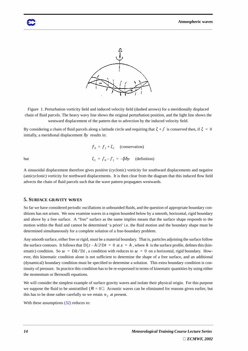
Figure 1. Perturbation vorticity field and induced velocity field (dashed arrows) for a meridionally displaced
chain of fluid parcels. The heavy wavy line shows the original perturbation position, and the light line shows the
westward displacement of the pattern due to advection by the induced velocity field.
By consideringachainof fluid parcelsalonga latitudecircleandrequiringthat is conservedthen,if
initially, a meridional displacement results in:
but
A sinusoidaldisplacementthereforegivespositive (cyclonic) vorticity for southwarddisplacementsandnegative
(anticyclonic) vorticity for northwarddisplacements.It is thenclearfrom thediagramthatthis inducedflow field
advects the chain of fluid parcels such that the wave pattern propagates westwards.
5. SURFACE GRAVITY WAVES
Sofarwehaveconsideredperiodicoscillationsin unboundedfluids,andthequestionof appropriateboundarycon-
ditionshasnotarisen.Wenow examinewavesin aregionboundedbelow by asmooth,horizontal,rigid boundary
andabove by a freesurface. A “free” surfaceasthenameimpliesmeansthat thesurfaceshaperespondsto the
motionwithin thefluid andcannotbedetermined‘a priori' i.e. thefluid motionandtheboundaryshapemustbe
determined simultaneously for a complete solution of a free-boundary problem.
Any smoothsurface,eitherfreeor rigid, mustbeamaterialboundary. Thatis,particlesadjoiningthesurfacefollow
thesurfacecontours.It followsthat at , where is thesurfaceprofile,definesthis(kin-
ematic)condition. So , a conditionwith reducesto on a horizontal,rigid boundary. How-
ever, this kinematicconditionaloneis not sufficient to determinethe shapeof a free surface,andan additional
(dynamical)boundaryconditionmustbespecifiedto determinea solution. This extra boundaryconditionis con-
tinuity of pressure.In practicethisconditionhasto bere-expressedin termsof kinematicquantitiesby usingeither
the momentum or Bernoulli equations.
Wewill considerthesimplestexampleof surfacegravity wavesandisolatetheirphysicalorigin. For thispurpose
we supposethefluid to beunstratified . Acousticwavescanbeeliminatedfor reasonsgivenearlier, but
this has to be done rather carefully so we retain at present.
With these assumptions(32) reduces to:
ζ �+ ζ 0=
δ�
� 0 � 1 ζ1 (conservation)+=
ζ1 � 0 � 1– βδ� (definition)–= =
D � 7–( ) D �⁄ 0= � 7= 7� D 7 D �⁄= � 0=
� 0=( ) �2
Atmospheric waves
Meteorological Training Course Lecture Series
ECMWF, 2002 15
(57)
For simplicity we will look at the behaviour of small amplitude waves in a fluid with a free surface
above which thepressureis assumedconstant(e.g.air–seainterface,modelof waves
on inversion). The lower boundary is assumed to be a rigid horizontal surface at .
With the above comments in mind the (non linear) boundary conditions are:
(i) at
(ii) at
(iii) pressurecontinuousat the free surface,which in this example is equivalent to at
.
The linearized forms of these conditions are:
(i) at
(ii) at
(iii) at which,by using(29)andtheconditionthat ,
can be shown to be equivalent to
(58)
From(58) we seethat if we eliminateacousticwavesby setting , we mustalsoset in the
boundaryconditionotherwiseanoscillation,spuriousin thesensethatit cannotoccurin theexactequations,will
arise through an inconsistent approximation.
Equation(57), with theabove boundaryconditions,canreadilybesolved for all wavelengthsbut it is
instructive to consider long and short waves independently.
5.1 Long waves
If wavesarelong to theextentthat and , thenthenon-hydrostatictermcontainingtheterm in
(57) can be neglected by comparison with and the solution is seen to be:
(59)
where .
� 2
2
d
d � ˆ�
1�0
------- �dd � ˆ– �
4σ2 2
σ2 � 2–-----------------
�2� 2
-----– � ˆ– 0=
7����,( )� � σ �+( )cos= � 0=
� 0= � 0=
� D 7 D �⁄= � 7=
D� D �⁄ 0=� 7=
δ � 0= � 0=
δ � ∂ 7 ∂ �⁄= � 7=
∂ δ� ρ0⁄( ) ∂ �⁄ � δ �= � 7= � � � 2⁄+ 1�
0⁄=
�dd � ˆ
�1�
2–( )�0
---------------------- � 2
σ2 � 2–-----------------+ � ˆ– 0 at � 7= =
�2
�3 0= = �
1 0=
� 0 1« 7 1« �4
1�
0⁄( ) 8,� ˆ 8 �⁄( )
δ � σ� 1 e
91 +:
0-------
–
e
91 ;:
0-------
1– --------------------------- � σ �+( )sin=
σ2 � 2 � � 0 2 1 e
91 ;:
0-------–
–
+=

Atmospheric waves
16 Meteorological Training Course Lecture Series
ECMWF, 2002
If the height scale is negligible by comparison with the density scale height left( )
andis, therefore,thepropagationspeedof long surfacewavesin a liquid or anatmosphericlayerwhich is much
shallower than 7 km. For instance, long waves on the boundary-layer inversion, km and so m s-1.
If, on the other hand, (for example in a deep gas) then .
It is easyto show that theearthsrotationonly becomesimportantfor synopticscalesor longer. For theearthsat-
mospherethesedeeplongwavespropagateatabout270m s-1. Theselongwavesareoftenreferredto as“shallow
water” waves and the equationset resulting from (17)–(21) with the relevant approximations(normally with
) form the “shallow waterequations”.Theseprovide a popularequationset for analytical/dynamical
studies and also for testing and designing numerical integration schemes.
5.2 Short waves
When and theterminvolving cannotbeneglectedwhereasrotationcanobviouslybeso. The
solution can be shown to be:
(60)
where . Hence for , , a much slower phase speed than the long waves.
If desired, free-surface waves can be eliminated by imposing rigid upper and lower boundary conditions.
6. EQUATORIAL WAVES
NeartheEquatoratmosphericwavesacquirearatherdifferentcharacterandwhatwereclearlydistinctmechanisms
ceaseto beso. Following Matsuno(1966)wewill studyequatorialwavesusingtheshallow waterequationswith
, known astheequatorialbeta-plane,andincluding , andlinearizeagainaboutastateof nomo-
tion. Hence:
(61)
EXERCISE:
7 �0«
σ ---
� 2
2----- � 7+
O7�
0-------
+=
7 1≈ � 100≈
7 �0» σ
---� 2
2----- � � 0+
=
∂ ∂�⁄ 0≠
� 0 1» 7 1» �4
δ � σ� �( )sinh
7( )sin---------------------- �
1
� 7–( )2�
0----------------- � σ �+( )sinexp–=
σ2 �, 7( )tanh= 7 1» σ ⁄ �< ⁄≈
� β�= ∂ ∂�⁄ 0≠
∂ '∂ �-------- β� � '– � ∂ 7 '
∂�--------+ = 0
∂ � '∂ �------- β� ' � ∂ 7 ′
∂�--------+ + = 0
∂ 7 ′∂ �--------
� ∂ '∂�-------- ∂ � '
∂�-------+ + = 0
Atmospheric waves
Meteorological Training Course Lecture Series
ECMWF, 2002 17
Derive the above equations from(1)–(5).
Assumingwavelikeformsfor in theeast–westdirection,but retainingthe
-variation explicitly leads to the differential equation:
(62)
It is convenient to non-dimensionalize the equation using:
(62) then becomes:
(63)
This equation is a form of Schrödinger equation with solutions, if
, (64)
of the form ,
where is an th order Hermite polynomial ( ).
Clearly the solutions are 'trapped' near the Equator by the Gaussian function .
The dispersion or frequency relationship(64) is cubic in :
(65)
Thethreedistinctrootsrepresentapairof inertialgravity wavesandoneRossbywave. Thesolutionscanconven-
iently be studied by considering the cases (a) and (b) ( large), hence:
(66)
(67)
Returning to dimensional variables, we obtain for the phase velocities (defined by ):
,
' � ' 7 ', ,( ) ˆ � ˆ 7 ˆ, ,( ) �! � σ �+( )[ ]exp=�
d2 � ˆd� 2--------- σ2
� �--------- 2– βσ
------β2
� �--------- y2–+ � ˆ+ 0=
� 2 � �β
-------------λ2 2;β� �-------------µ2 σ2; � � βω2= = =
8 2 � ˆ8 λ2--------- ω2 µ2– µ
ω---- λ2–+
� ˆ+ 0=
ω2 µ2– µω----+ 2� 1 ( �+ 0 1 2 … ), , ,= =
� ˆ � 0 λ2 2⁄–( ) = 9 λ( )exp=
= 9 � = 0 1 = 1, 2λ = 2, 2 2λ2 1–( )= = =
λ2 2⁄–( )exp
ω
ω3 µ2 2� 1+ +( )ω– µ+ 0=
ω2 µ2∼ ω µ«
ω1 2, µ2 2� 1+ ++−=
ω3µ
µ2 2� 1+ +----------------------------=
� σ ⁄–≡
�1 2, � � 1 β 2� 1+( )
2 � �------------------------++−=
�3
β
2 β 2� 1+( )� �------------------------+
------------------------------------------–=

Atmospheric waves
18 Meteorological Training Course Lecture Series
ECMWF, 2002
Obviously area pair of eastward andwestward propagating inertial gravity waveswhile is a westward
propagating Rossby wave.
For these three solutions are distinct but for , (65) can be factorized:
Theroot is unacceptable(show) but theroot is aneastwardpropagatingin-
ertialgravity waveandtherootomega is calledamixedRossbygravity wave; this is
because,as (thelimiting caseof gravity waves(see(66)), while, as , thelimit-
ing case of Rossby waves (see(67)).
Oneotherimportantspecialcaseis when . This correspondsto a wave with identicallyzero.This has
solutions(see(61)) , whereonly thepositive root is acceptable(thenegative root violates
theequatorialbeta-planeassumption.Seealso(65) with ). This fast-moving eastwardpropagatingwave
is theKelvin wave (seeFig. 2 ). Thesewavesoccurcommonlyin theoceanaswavesalongcoastlines(decaying
exponentially away from the coast).
Figure 2. Velocityandpressuredistributionsin thehorizontalplanefor (a)Kelvin waves,and(b) Rossby–gravity
waves (from Matsuno “Quasi-geostrophic motions in the equatorial area”, J. Meteorol. Soc. Japan, 1966).
Datastudiesof theequatorialstratospherehave identifiedbothvery long wavelengthKelvin andmixedRossby–
gravity waves.Considerablerecentinteresthasbeenshown in thesetropicalwavesin studiesof diabaticforcing in
thetropicsandits impactonhigherlatitudes(Gill , 1980etc.).Fig. 3 summarisestheseequatorialwavecharacter-
istics.
�1 2,
�3
� 1≥ � 0=
ω µ–( ) ω2 ωµ 1–+( ) 0=
ω µ= ω1 µ 2⁄– µ 2⁄( )2 1+–=
ω2 µ 2⁄– µ 2⁄( )2 1++=
µ 0 ω2 1→,→ µ ∞ ω2 0→,→
� 1–= � ˆ� σ ⁄– � �±= = � 1–=

Atmospheric waves
Meteorological Training Course Lecture Series
ECMWF, 2002 19
Figure 3. Non-dimensionalfrequenciesfrom (65)asa functionof wavenumber. Thelinesindicatethefollowing
types of waves: Eastward propagating inertial–gravity wave (thin solid line); westward propagating inertial–
gravity wave (thin dashedline); Rossbywave (thick solid line); Kelvin wave (thick dashedline). (After Matsuno
1966)

Atmospheric waves
20 Meteorological Training Course Lecture Series
ECMWF, 2002
7. SUMMAR Y DIAGRAM AND MODELLING IMPLICA TIONS
Figure 4. Waves in a compressible atmosphere (from J. S. A. Green — Dynamics lecture notes)
Fig. 4 summarisesthebasicwave types.It is adispersiondiagramof horizontalphasespeedplottedagainsthori-
zontalwavelength(bothlogarithmicscales)soisoplethsof wave periodarestraightlinesof unit slopewith inter-
cept . Some points of interest are:
(i) The short vertical wavelengthacousticwaves which, while having phasespeedsnormal to their
wave frontsequalto , havevery largehorizontalphasespeeds(with wave frontsalmost
parallel to the ground).
(ii) Mesoscale gravity waves are almost non-dispersive.
(iii) Rossbywavesfor long wavelengthsvary like while theshorterwavelengthsincludethemixed
Rossby-gravity mode.
In previoussectionswe have identifiedseveralwave typeswith a wide rangeof frequencies.Thechoiceof time
stepin anumericalmodelis dominatedby thehighestfrequency waves(seeLectureNote1.4).Thusfor example,
acousticwaveshave a frequency andfor a typical large-scalemodel .
Hence is dominatedby theverticallypropagatingacousticwavesandit is desirableto filter out theseverti-
cally propagating waves by assuming hydrostatic balance.
σlog
� ��
=
2–
σ � 2 - 2+= -⁄ ∆� ∆�⁄ 10 2–∼=
σMAX

Atmospheric waves
Meteorological Training Course Lecture Series
ECMWF, 2002 21
Horizontallypropagatingacousticwaves(Lamb)poselessof aproblemsincetheirfrequenciesarenotmuchhigher
thanthe long gravity wavesdiscussedearlierleft ( ). Neverthelessvariousnumerical
techniques have been devised to ease this restriction (see Lecture Note 1.4).
Wecouldmaketheanelasticapproximation( in thecontinuityequation)but retainthenon-hydrostat-
ic terms.An equationsetbasedon(17)–(21)with thenallowsusto predict , and ; however
thesecomponentsmustsatisfythecontinuityequation.Differentiating(20) with respectto time andsubstituting
from (17), (18) and (19) gives a diagnostic Poisson-type equation for the pressure of the form
which mustbe invertedeachtime step.This is a relatively expensive procedure
andnotjustifiablefor large-scalemodelsbecausethehydrostaticapproximationis well-satisfied.For muchsmaller
scalemodelswhere thedecisionis no longerstraightforwardandgenerallyeithertheanelasticapproxi-
mation is made or sound waves are retained and treated by some sophisticated numerical technique.
REFERENCES
Gill , A. E.,1980:Somesimplesolutionsfor heat-inducedtropicalcirculation.Quart.J.Roy. Meteor. Soc.,106, 447
- 462.
Haltiner, E. andWilliams, R. T., 1980:NumericalPredictionandDynamicMeteorology. 2ndEdition.Wiley, 477
pp.
Holton, J.R.,1972:An introductionto dynamicmeteorology. InternationalGeophysicalSeries,Vol. 16,Academic
Press, 319 pp.
Kasahara, 1974:Variousverticalcoordinatesystemsusedfor numericalweatherprediction.Mon. Wea.Rev., 102,
509 - 522.
Matsuno, 1966: Quasi-geostrophic motions in the equatorial area. J. Met. Soc. Japan,44, 25 - 43.
Miller, M. J.1974:On theuseof pressureasverticalcoordinatein modellingconvection. Quart.J.Roy. Meteor.
Soc.,100, 155 - 162.
Miller, M. J.andWhite,A. A. 1984:On thenon-hydrostaticequationsin pressureandsigmacoordinates.Quart.
J. Roy. Meteor. Soc.,110, 515 - 535.
ACKNOWLEDGEMENTS
Thesenotesrely heavily on unpublishedlecturenoteswritten by J.S.A. Greenwith subsequentmodificationsby
M. W. Moncrieff. Additional material was gleaned from a number of referenced sources.
σa( ) σg⁄ γ��� � �⁄ 1≥∼
∂ρ ∂ �⁄ 0=�2
�3 0= = � �
∇2 δ� ρ0⁄( ) >?@�A� …, , ,( )=
∆ � ∆�≥