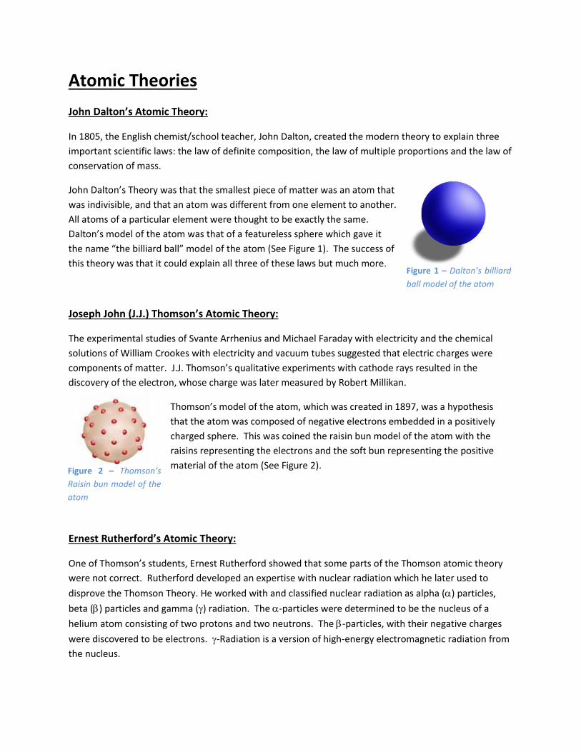
Figure 2 – Thomson’s

Raisin bun model of the

atom

Atomic Theories

John Dalton’s Atomic Theory:

In 1805, the English chemist/school teacher, John Dalton, created the modern theory to explain three

important scientific laws: the law of definite composition, the law of multiple proportions and the law of

conservation of mass.

John Dalton’s Theory was that the smallest piece of matter was an atom that

was indivisible, and that an atom was different from one element to another.

All atoms of a particular element were thought to be exactly the same.

Dalton’s model of the atom was that of a featureless sphere which gave it

the name “the billiard ball” model of the atom (See Figure 1). The success of

this theory was that it could explain all three of these laws but much more.

Joseph John (J.J.) Thomson’s Atomic Theory:

The experimental studies of Svante Arrhenius and Michael Faraday with electricity and the chemical

solutions of William Crookes with electricity and vacuum tubes suggested that electric charges were

components of matter. J.J. Thomson’s qualitative experiments with cathode rays resulted in the

discovery of the electron, whose charge was later measured by Robert Millikan.

Thomson’s model of the atom, which was created in 1897, was a hypothesis

that the atom was composed of negative electrons embedded in a positively

charged sphere. This was coined the raisin bun model of the atom with the

raisins representing the electrons and the soft bun representing the positive

material of the atom (See Figure 2).

Ernest Rutherford’s Atomic Theory:

One of Thomson’s students, Ernest Rutherford showed that some parts of the Thomson atomic theory

were not correct. Rutherford developed an expertise with nuclear radiation which he later used to

disprove the Thomson Theory. He worked with and classified nuclear radiation as alpha () particles,

beta () particles and gamma () radiation. The -particles were determined to be the nucleus of a

helium atom consisting of two protons and two neutrons. The -particles, with their negative charges

were discovered to be electrons. -Radiation is a version of high-energy electromagnetic radiation from

the nucleus.

Figure 1 – Dalton’s billiard

ball model of the atom

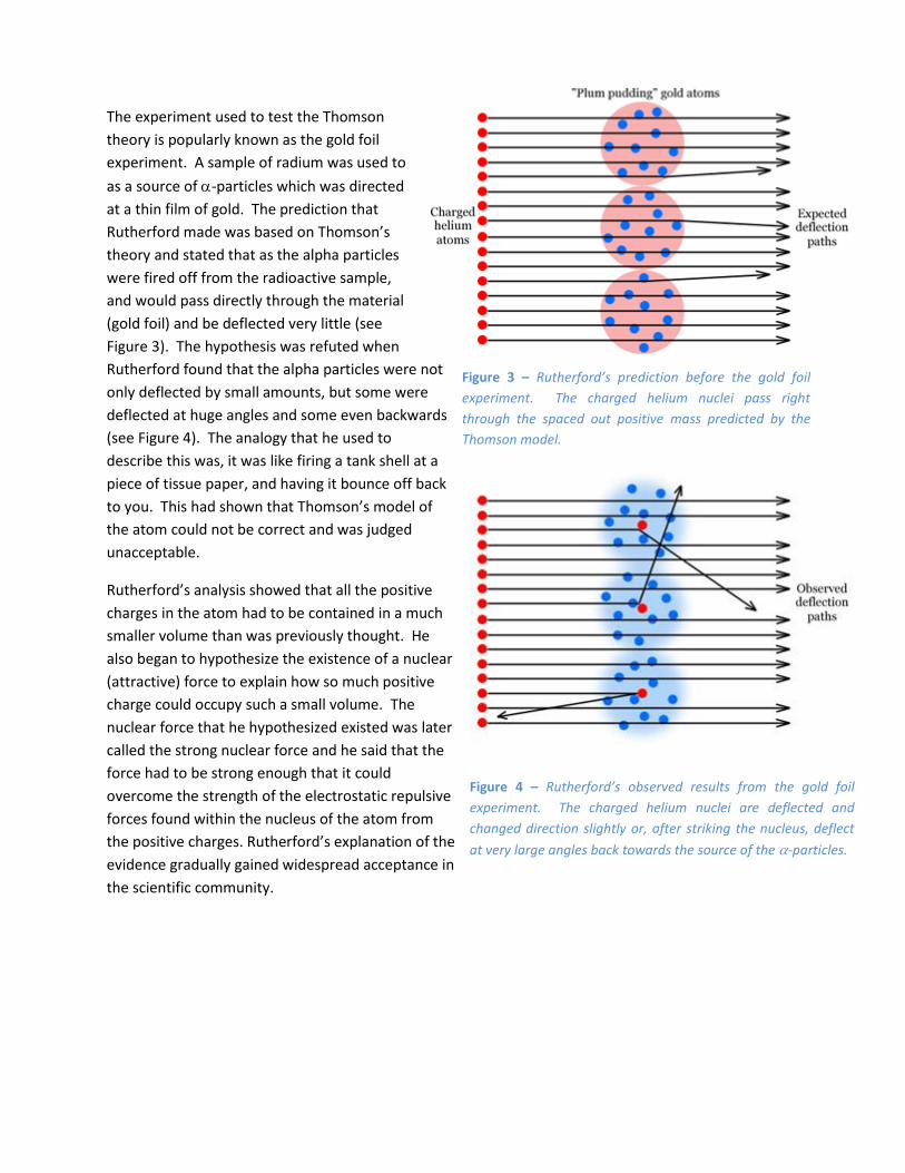
Figure 3 – Rutherford’s prediction before the gold foil

experiment. The charged helium nuclei pass right

through the spaced out positive mass predicted by the

Thomson model.

The experiment used to test the Thomson

theory is popularly known as the gold foil

experiment. A sample of radium was used to

as a source of -particles which was directed

at a thin film of gold. The prediction that

Rutherford made was based on Thomson’s

theory and stated that as the alpha particles

were fired off from the radioactive sample,

and would pass directly through the material

(gold foil) and be deflected very little (see

Figure 3). The hypothesis was refuted when

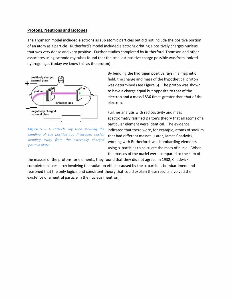
Rutherford found that the alpha particles were not

only deflected by small amounts, but some were

deflected at huge angles and some even backwards

(see Figure 4). The analogy that he used to

describe this was, it was like firing a tank shell at a

piece of tissue paper, and having it bounce off back

to you. This had shown that Thomson’s model of

the atom could not be correct and was judged

unacceptable.

Rutherford’s analysis showed that all the positive

charges in the atom had to be contained in a much

smaller volume than was previously thought. He

also began to hypothesize the existence of a nuclear

(attractive) force to explain how so much positive

charge could occupy such a small volume. The

nuclear force that he hypothesized existed was later

called the strong nuclear force and he said that the

force had to be strong enough that it could

overcome the strength of the electrostatic repulsive

forces found within the nucleus of the atom from

the positive charges. Rutherford’s explanation of the

evidence gradually gained widespread acceptance in

the scientific community.

Figure 4 – Rutherford’s observed results from the gold foil

experiment. The charged helium nuclei are deflected and

changed direction slightly or, after striking the nucleus, deflect

at very large angles back towards the source of the -particles.

Protons, Neutrons and Isotopes

The Thomson model included electrons as sub atomic particles but did not include the positive portion

of an atom as a particle. Rutherford’s model included electrons orbiting a positively charges nucleus

that was very dense and very positive. Further studies completed by Rutherford, Thomson and other

associates using cathode ray tubes found that the smallest positive charge possible was from ionized

hydrogen gas (today we know this as the proton).

By bending the hydrogen positive rays in a magnetic

field; the charge and mass of the hypothetical proton

was determined (see Figure 5). The proton was shown

to have a charge equal but opposite to that of the

electron and a mass 1836 times greater than that of the

electron.

Further analysis with radioactivity and mass

spectrometry falsified Dalton’s theory that all atoms of a

particular element were identical. The evidence

indicated that there were, for example, atoms of sodium

that had different masses. Later, James Chadwick,

working with Rutherford, was bombarding elements

using -particles to calculate the mass of nuclei. When

the masses of the nuclei were compared to the sum of

the masses of the protons for elements, they found that they did not agree. In 1932, Chadwick

completed his research involving the radiation effects caused by the -particles bombardment and

reasoned that the only logical and consistent theory that could explain these results involved the

existence of a neutral particle in the nucleus (neutron).

Figure 5 – A cathode ray tube showing the

bending of the positive ray (hydrogen nuclei)

bending away from the externally charged

positive plate.

The Origins of Quantum Theory

Black Body Radiation

As a solid is heated to higher and higher temperatures, it begins to glow. Initially, it appears red and

then become white when the temperatures increase to higher levels. Since white light is a combination

of all the colours, the light emitted by the hotter object, must be accompanied by, for example, blue

light. The changes in the colours and the corresponding spectra do not depend on the composition of

the solid.

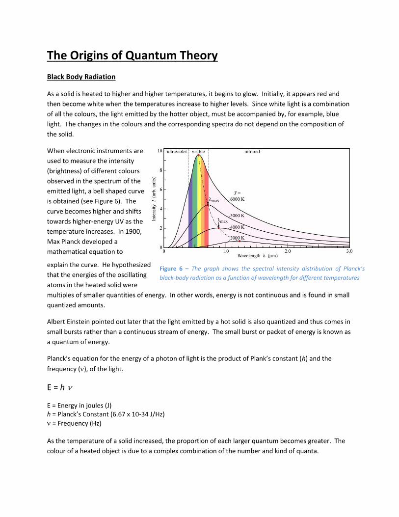
When electronic instruments are

used to measure the intensity

(brightness) of different colours

observed in the spectrum of the

emitted light, a bell shaped curve

is obtained (see Figure 6). The

curve becomes higher and shifts

towards higher-energy UV as the

temperature increases. In 1900,

Max Planck developed a

mathematical equation to

explain the curve. He hypothesized

that the energies of the oscillating

atoms in the heated solid were

multiples of smaller quantities of energy. In other words, energy is not continuous and is found in small

quantized amounts.

Albert Einstein pointed out later that the light emitted by a hot solid is also quantized and thus comes in

small bursts rather than a continuous stream of energy. The small burst or packet of energy is known as

a quantum of energy.

Planck’s equation for the energy of a photon of light is the product of Plank’s constant (h) and the

frequency (), of the light.

E = h

E = Energy in joules (J) h = Planck’s Constant (6.67 x 10-34 J/Hz)

= Frequency (Hz) As the temperature of a solid increased, the proportion of each larger quantum becomes greater. The

colour of a heated object is due to a complex combination of the number and kind of quanta.

Figure 6 – The graph shows the spectral intensity distribution of Planck’s

black-body radiation as a function of wavelength for different temperatures

The Photoelectric Effect

Greek philosophers believed that light was a stream of particles. Christian Huygens proposed that light

can be best described as a wave. Isaac Newton, the famous English scientist, opposed Huygens view

and continued to try to explain the properties of light in terms of minute particle which he called

corpuscles.

Mounting evidence from scientists with reflections, refractions and diffraction favoured the wave

hypothesis. James Maxwell proposed that light is an electromagnetic wave composed of electric and

magnetic fields that can exert forces on charged particles. The electromagnetic wave theory, known as

the classical theory of light, became widely accepted when new experiments supported this view.

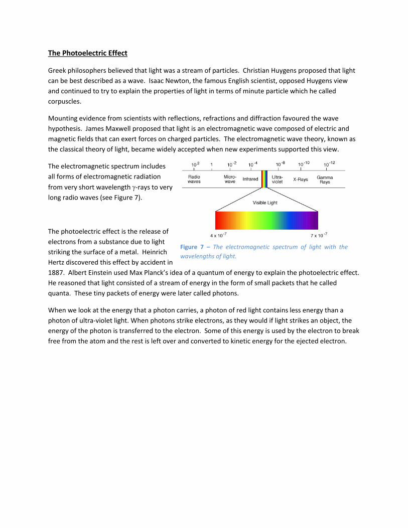
The electromagnetic spectrum includes

all forms of electromagnetic radiation

from very short wavelength -rays to very

long radio waves (see Figure 7).

The photoelectric effect is the release of

electrons from a substance due to light

striking the surface of a metal. Heinrich

Hertz discovered this effect by accident in

1887. Albert Einstein used Max Planck’s idea of a quantum of energy to explain the photoelectric effect.

He reasoned that light consisted of a stream of energy in the form of small packets that he called

quanta. These tiny packets of energy were later called photons.

When we look at the energy that a photon carries, a photon of red light contains less energy than a

photon of ultra-violet light. When photons strike electrons, as they would if light strikes an object, the

energy of the photon is transferred to the electron. Some of this energy is used by the electron to break

free from the atom and the rest is left over and converted to kinetic energy for the ejected electron.

Figure 7 – The electromagnetic spectrum of light with the

wavelengths of light.

The Bohr Atomic Theory

Atomic Spectra

Ernest Rutherford and other scientists had guessed that the electrons move around the nucleus as

planets orbit the sun. An electron traveling in a circular orbit is constantly changing its directions, and

thus accelerating. According to the classical theory, the orbiting electron should emit photons of

electromagnetic radiation, losing energy in the process, and thus spiraling inwards towards the nucleus,

collapsing the atom. This prediction was obviously incorrect as we are here reading this document.

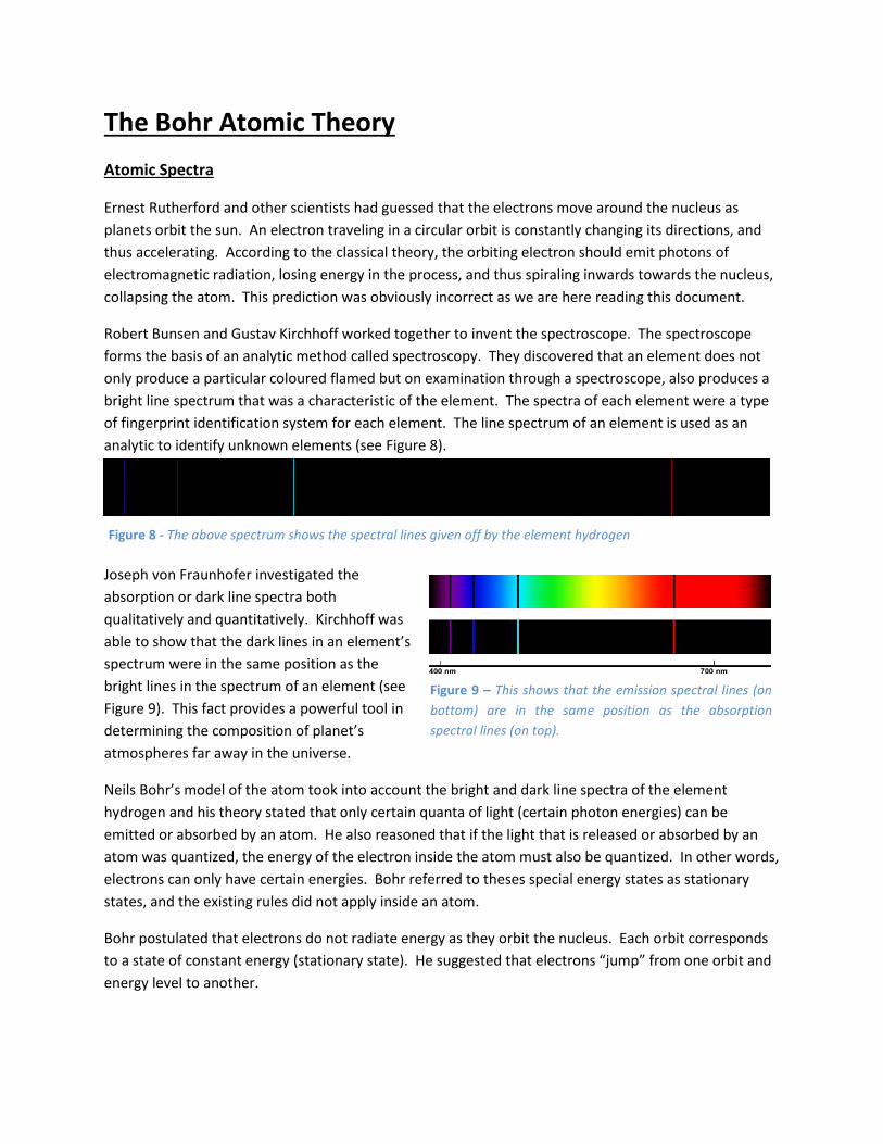
Robert Bunsen and Gustav Kirchhoff worked together to invent the spectroscope. The spectroscope

forms the basis of an analytic method called spectroscopy. They discovered that an element does not

only produce a particular coloured flamed but on examination through a spectroscope, also produces a

bright line spectrum that was a characteristic of the element. The spectra of each element were a type

of fingerprint identification system for each element. The line spectrum of an element is used as an

analytic to identify unknown elements (see Figure 8).

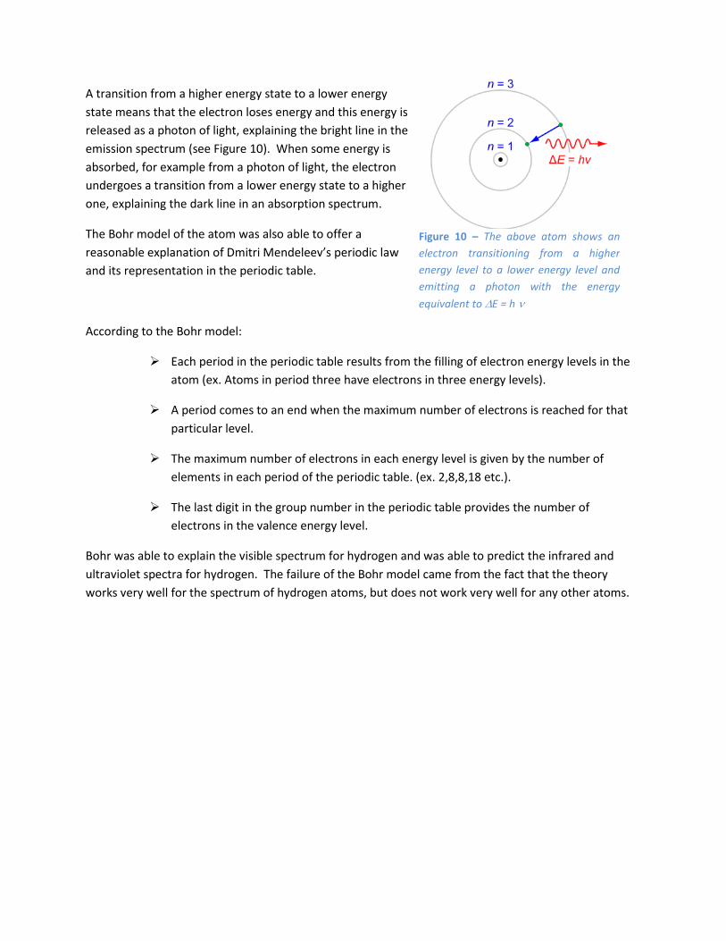
Joseph von Fraunhofer investigated the

absorption or dark line spectra both

qualitatively and quantitatively. Kirchhoff was

able to show that the dark lines in an element’s

spectrum were in the same position as the

bright lines in the spectrum of an element (see

Figure 9). This fact provides a powerful tool in

determining the composition of planet’s

atmospheres far away in the universe.

Neils Bohr’s model of the atom took into account the bright and dark line spectra of the element

hydrogen and his theory stated that only certain quanta of light (certain photon energies) can be

emitted or absorbed by an atom. He also reasoned that if the light that is released or absorbed by an

atom was quantized, the energy of the electron inside the atom must also be quantized. In other words,

electrons can only have certain energies. Bohr referred to theses special energy states as stationary

states, and the existing rules did not apply inside an atom.

Bohr postulated that electrons do not radiate energy as they orbit the nucleus. Each orbit corresponds

to a state of constant energy (stationary state). He suggested that electrons “jump” from one orbit and

energy level to another.

Figure 8 - The above spectrum shows the spectral lines given off by the element hydrogen

Figure 9 – This shows that the emission spectral lines (on

bottom) are in the same position as the absorption

spectral lines (on top).

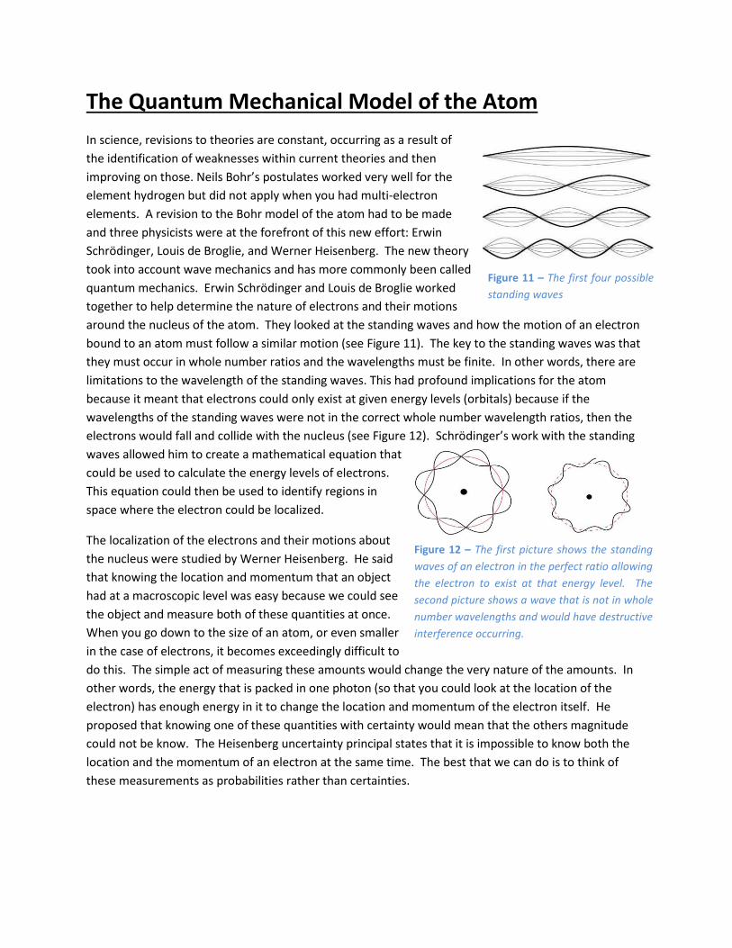
A transition from a higher energy state to a lower energy

state means that the electron loses energy and this energy is

released as a photon of light, explaining the bright line in the

emission spectrum (see Figure 10). When some energy is

absorbed, for example from a photon of light, the electron

undergoes a transition from a lower energy state to a higher

one, explaining the dark line in an absorption spectrum.

The Bohr model of the atom was also able to offer a

reasonable explanation of Dmitri Mendeleev’s periodic law

and its representation in the periodic table.

According to the Bohr model:

➢ Each period in the periodic table results from the filling of electron energy levels in the

atom (ex. Atoms in period three have electrons in three energy levels).

➢ A period comes to an end when the maximum number of electrons is reached for that

particular level.

➢ The maximum number of electrons in each energy level is given by the number of

elements in each period of the periodic table. (ex. 2,8,8,18 etc.).

➢ The last digit in the group number in the periodic table provides the number of

electrons in the valence energy level.

Bohr was able to explain the visible spectrum for hydrogen and was able to predict the infrared and

ultraviolet spectra for hydrogen. The failure of the Bohr model came from the fact that the theory

works very well for the spectrum of hydrogen atoms, but does not work very well for any other atoms.

Figure 10 – The above atom shows an

electron transitioning from a higher

energy level to a lower energy level and

emitting a photon with the energy

equivalent to E = h

The Quantum Mechanical Model of the Atom

In science, revisions to theories are constant, occurring as a result of

the identification of weaknesses within current theories and then

improving on those. Neils Bohr’s postulates worked very well for the

element hydrogen but did not apply when you had multi-electron

elements. A revision to the Bohr model of the atom had to be made

and three physicists were at the forefront of this new effort: Erwin

Schrödinger, Louis de Broglie, and Werner Heisenberg. The new theory

took into account wave mechanics and has more commonly been called

quantum mechanics. Erwin Schrödinger and Louis de Broglie worked

together to help determine the nature of electrons and their motions

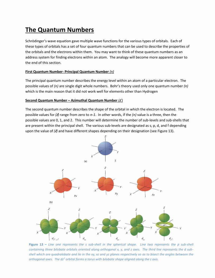
around the nucleus of the atom. They looked at the standing waves and how the motion of an electron

bound to an atom must follow a similar motion (see Figure 11). The key to the standing waves was that

they must occur in whole number ratios and the wavelengths must be finite. In other words, there are

limitations to the wavelength of the standing waves. This had profound implications for the atom

because it meant that electrons could only exist at given energy levels (orbitals) because if the

wavelengths of the standing waves were not in the correct whole number wavelength ratios, then the

electrons would fall and collide with the nucleus (see Figure 12). Schrödinger’s work with the standing

waves allowed him to create a mathematical equation that

could be used to calculate the energy levels of electrons.

This equation could then be used to identify regions in

space where the electron could be localized.

The localization of the electrons and their motions about

the nucleus were studied by Werner Heisenberg. He said

that knowing the location and momentum that an object

had at a macroscopic level was easy because we could see

the object and measure both of these quantities at once.

When you go down to the size of an atom, or even smaller

in the case of electrons, it becomes exceedingly difficult to

do this. The simple act of measuring these amounts would change the very nature of the amounts. In

other words, the energy that is packed in one photon (so that you could look at the location of the

electron) has enough energy in it to change the location and momentum of the electron itself. He

proposed that knowing one of these quantities with certainty would mean that the others magnitude

could not be know. The Heisenberg uncertainty principal states that it is impossible to know both the

location and the momentum of an electron at the same time. The best that we can do is to think of

these measurements as probabilities rather than certainties.

Figure 11 – The first four possible

standing waves

Figure 12 – The first picture shows the standing

waves of an electron in the perfect ratio allowing

the electron to exist at that energy level. The

second picture shows a wave that is not in whole

number wavelengths and would have destructive

interference occurring.

The Quantum Numbers

Schrödinger’s wave equation gave multiple wave functions for the various types of orbitals. Each of

these types of orbitals has a set of four quantum numbers that can be used to describe the properties of

the orbitals and the electrons within them. You may want to think of these quantum numbers as an

address system for finding electrons within an atom. The analogy will become more apparent closer to

the end of this section.

First Quantum Number- Principal Quantum Number (n)

The principal quantum number describes the energy level within an atom of a particular electron. The

possible values of (n) are single digit whole numbers. Bohr’s theory used only one quantum number (n)

which is the main reason that it did not work well for elements other than Hydrogen

Second Quantum Number – Azimuthal Quantum Number (l )

The second quantum number describes the shape of the orbital in which the electron is located. The

possible values for (l) range from zero to n-1. In other words, if the (n) value is a three, then the

possible values are 0, 1, and 2. This number will determine the number of sub-levels and sub-shells that

are present within the principal shell. The various sub-levels are designated as s, p, d, and f depending

upon the value of (l) and have different shapes depending on their designation (see Figure 13).

Figure 13 – Line one represents the s sub-shell in the spherical shape. Line two represents the p sub-shell

containing three bilobate orbitals oriented along orthogonal x, y, and z axes. The third line represents the d sub-

shell which are quadralobate and lie in the xy, xz and yz planes respectively so as to bisect the angles between the

orthogonal axes. The dz2 orbital forms a torus with bilobate shape aligned along the z axis.

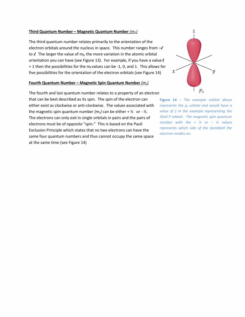
Third Quantum Number – Magnetic Quantum Number (ml )

The third quantum number relates primarily to the orientation of the

electron orbitals around the nucleus in space. This number ranges from –l

to l. The larger the value of ml, the more variation in the atomic orbital

orientation you can have (see Figure 13). For example, if you have a value l

= 1 then the possibilities for the ml values can be -1, 0, and 1. This allows for

five possibilities for the orientation of the electron orbitals (see Figure 14)

Fourth Quantum Number – Magnetic Spin Quantum Number (ms)

The fourth and last quantum number relates to a property of an electron

that can be best described as its spin. The spin of the electron can

either exist as clockwise or anti-clockwise. The values associated with

the magnetic spin quantum number (ms) can be either + ½ or - ½.

The electrons can only exit in single orbitals in pairs and the pairs of

electrons must be of opposite “spin.” This is based on the Pauli

Exclusion Principle which states that no two electrons can have the

same four quantum numbers and thus cannot occupy the same space

at the same time (see Figure 14)

Figure 14 – The example orbital above

represents the pz orbital and would have a

value of 1 in the example representing the

third P orbital. The magnetic spin quantum

number with the + ½ or – ½ values

represents which side of the dumbbell the

electron resides on.

Orbital Diagrams

In order to show the energy distribution of electrons in an atom, we have developed orbital diagrams

that not only show which orbitals are filled, but also the location and energy of the electrons. They are

helpful to us to understand where electrons are, and from where they can be removed or added to

atoms. They are also a way of pictorially representing the four quantum numbers that we have learned

about. There are some rules to consider before we begin with our orbital diagrams and these rules are

fundamental rules when constructing our diagrams. Included in this are examples of energy level

diagrams (see Figure 16). They cannot be broken!

Pauli Exclusion Principle:

The Pauli Exclusion Principle states that no two electrons in an atom can have

the same four quantum numbers and as a result cannot occupy the same

location in space. The electron repulsion pressures hold up and do not allow

this to happen. This is also the reason that atoms can be so vast with over 99%

of the atom open space, with infinitesimally small particles making up the atom,

and yet be solid at the macroscopic level (it is why we do not fall through the

floor as we stand here reading this page).

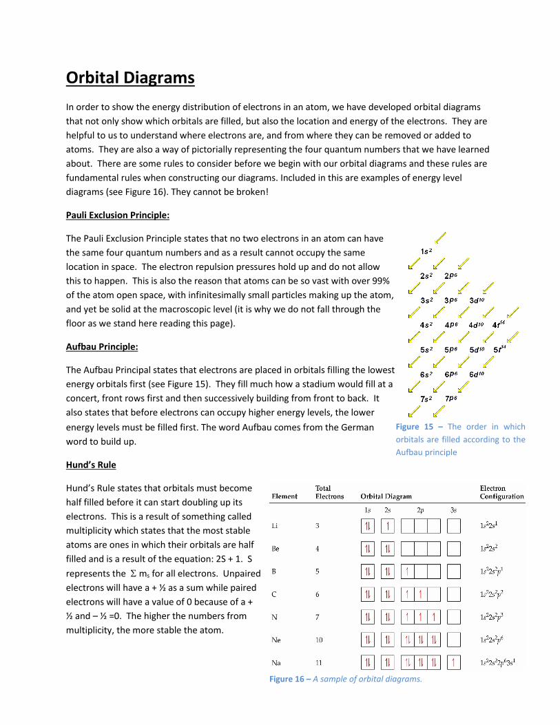
Aufbau Principle:

The Aufbau Principal states that electrons are placed in orbitals filling the lowest

energy orbitals first (see Figure 15). They fill much how a stadium would fill at a

concert, front rows first and then successively building from front to back. It

also states that before electrons can occupy higher energy levels, the lower

energy levels must be filled first. The word Aufbau comes from the German

word to build up.

Hund’s Rule

Hund’s Rule states that orbitals must become

half filled before it can start doubling up its

electrons. This is a result of something called

multiplicity which states that the most stable

atoms are ones in which their orbitals are half

filled and is a result of the equation: 2S + 1. S

represents the ms for all electrons. Unpaired

electrons will have a + ½ as a sum while paired

electrons will have a value of 0 because of a +

½ and – ½ =0. The higher the numbers from

multiplicity, the more stable the atom.

Figure 16 – A sample of orbital diagrams.

Figure 15 – The order in which

orbitals are filled according to the

Aufbau principle

Electron Configurations

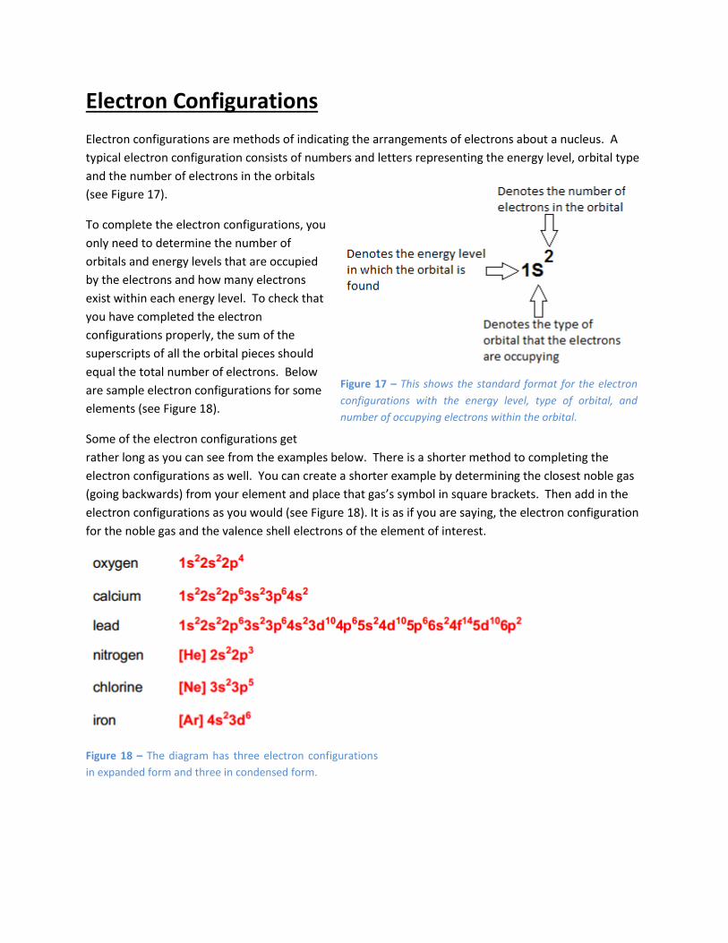
Electron configurations are methods of indicating the arrangements of electrons about a nucleus. A

typical electron configuration consists of numbers and letters representing the energy level, orbital type

and the number of electrons in the orbitals

(see Figure 17).

To complete the electron configurations, you

only need to determine the number of

orbitals and energy levels that are occupied

by the electrons and how many electrons

exist within each energy level. To check that

you have completed the electron

configurations properly, the sum of the

superscripts of all the orbital pieces should

equal the total number of electrons. Below

are sample electron configurations for some

elements (see Figure 18).

Some of the electron configurations get

rather long as you can see from the examples below. There is a shorter method to completing the

electron configurations as well. You can create a shorter example by determining the closest noble gas

(going backwards) from your element and place that gas’s symbol in square brackets. Then add in the

electron configurations as you would (see Figure 18). It is as if you are saying, the electron configuration

for the noble gas and the valence shell electrons of the element of interest.

Figure 17 – This shows the standard format for the electron

configurations with the energy level, type of orbital, and

number of occupying electrons within the orbital.

Figure 18 – The diagram has three electron configurations

in expanded form and three in condensed form.