Embed Size (px)
Citation preview

Attending kindergarten improves cognitive but not
socioemotional development in India∗
Joshua T. Dean Seema Jayachandran
University of Chicago Booth School of Business Northwestern University
November 17, 2019
Abstract
Pre-primary schooling is available but has low participation in many developing coun-
tries, which could exacerbate the socioeconomic gradient in readiness for primary
school. We study the effects of expanding access to kindergarten on child develop-
ment in Karnataka, India, through a randomized evaluation. We partnered with a
private kindergarten provider to offer two-year scholarships to children in low-income
families. Children who attend our partner’s kindergarten due to the scholarship expe-
rience a 0.8 standard deviation gain in cognitive development. About 40% of the effect
persists through the first year of primary school. We find no effect on socioemotional
development. Some children induced to attend our partner’s kindergarten would have
attended no kindergarten, while others would have attended a different kindergarten.
We use machine learning techniques to predict each child’s counterfactual activity and
then estimate separate treatment effects for different types of switchers. The short-run
effect on cognition is driven by children who would not have otherwise attended kinder-
garten, but the persistent component of the effect does not vary by counterfactual.
∗We thank UBS Optimus Foundation for funding this research; Tvisha Nevatia, Sadish Dhakal, Aditya Madhusudan, Akhila
Kovvuri, Sachet Bangia, Alejandro Favela, Ricardo Dahis, and Ariella Park for research assistance; and Azzurra Ruggeri for
advising us on measurement of child development. This study was preregistered in the AEA Trial Registry as AEARCTR-
0001078.

1 Introduction
Expanding access to pre-primary education has emerged as one of the next policy pri-
orities for developing countries, most of which have made great progress toward universal
enrollment in primary education in recent decades. Government-provided or subsidized
kindergarten and pre-kindergarten remain rare in developing countries. At the same time,
there is a growing consensus on the importance of the pre-primary years for children’s de-
velopment (Almond and Currie, 2011).
Most evidence on the impacts of pre-primary schooling is from developed countries,
but there are several reasons these estimates might not extrapolate to developing countries.
First, the quality of instruction might differ. Second, the effect size depends on how much
cognitive stimulation occurs through the counterfactual activity, such as home care, and
this will vary across contexts. Third, the persistence of the gains will depend on how much
remedial help primary schools give to lagging students; the tendency to “teach to the top” in
developing countries could make the effects of pre-primary schooling particularly persistent.
In this paper, we partner with a large, private provider of kindergarten, Hippocampus
Learning Centers (HLC), in Karnataka, India to evaluate how attending formal kindergarten
affects cognitive and socioemotional development. HLC runs kindergartens in over 200 vil-
lages. We randomly allocate scholarships to attend HLC, which cover 80-90% of the cost for
two years, among a sample of 808 children across 71 villages. The scholarship offer increases
the likelihood of attending HLC by 47 percentage points and the likelihood of attending
kindergarten at all by 20 percentage points.
We find that attending HLC has a large positive effect on cognitive development. At the
end of kindergarten, children induced to attend HLC by the scholarship score 0.8 standard
deviations higher than their peers on cognitive tests. This is the same magnitude as the
growth in scores over the two years among those in the control group who do not attend any
kindergarten between baseline and endline. The effect size attenuates by 60% by the end
of first grade, but the persistent component is still sizeable. This finding is similar to the
Head Start Impact Study which finds that about 45% of the effect persists from the end of
the second year of Head Start through the end of first grade (Kline and Walters, 2016); the
Head Start decline starts from a much smaller short-run effect size of 0.245, however.
We find no impact on socioemotional development, in either the short- or medium-run.
One potential explanation is that socioemotional skills arise through interacting with other
1

children in a structured environment, which the counterfactual activity also entails for most
children in our sample; attending public day care centers (anganwadis) is common.
We also decompose the effects by the child’s propensity to have attended kindergarten
even in the absence of our intervention. Understanding this heterogeneity is policy relevant
for two reasons. First, a government subsidy to attend kindergarten could likely target
families too poor to afford kindergarten better than we logistically were able to. The gains
to those who would not have otherwise attended kindergarten provides an upper bound on
the effect size a government might expect if it rolled out a similar program but with improved
targeting. Second, for logistical reasons we partnered with one provider, but a government
program would likely allow vouchers to be used at multiple providers. The treatment effect
on those who we induce to switch to HLC from a different kindergarten is a measure of how
much our partner outperforms or underperforms its competitors. Other questions about the
impacts of a scaled-up voucher program remain, such as how much the supply side would
expand in response to the increased demand, but the decomposition provides some important
extra facts to guide policy-making.
For the decomposition, we follow Crepon et al. (2019) and use machine learning tech-
niques to obtain a prediction of each child’s counterfactual attendance. The prediction
projects the control group’s actual behavior onto child- and village-level predetermined char-
acteristics. One advantage of the prospective nature of our study is that we could and did
ask parents at baseline what their plans were for the child’s care in the coming two years;
we can include these responses as predictors.
We then combine the prediction with a method proposed by Hull (2018) to obtain local
average treatment effects for two mutually exclusive types of compliers: those who would
have attended some kindergarten and those that would have attended none. We find that
attending HLC has a positive impact on cognitive development for both groups, but the effect
is much larger for those who would have otherwise not attended kindergarten (1.4 standard
deviations) than those who would have attended a non-HLC kindergarten (0.4 standard
deviations). When we decompose the end-of-first-grade effect, in contrast, we cannot reject
that the persistent component of the gains is the same for both groups.
2

2 Background
2.1 Pre-primary education in India
Enrollment in formal pre-primary schooling is quite limited in India; the gross enrollment
ratio in 2017 was 14% (UNESCO Institute of Statistics). The pre-primary education that
exists is offered by the private sector, without government funding. Most villages do have a
government-run anganwadi center, which provides around four hours a day of free child care
but does not offer instruction, e.g., with structured curriculum or by trained teachers.
The government’s role in pre-primary education in India in likely to expand in the near
future. In summer 2019, the Government of India released a draft proposal to include the
three years before entry into primary school under the Right to Education Act (Jebaraj,
2019). In the meantime, some states have already begun expanding their formal kinder-
garten capacity. For example, Karnataka announced in the summer of 2019 that it would be
opening 276 formal pre-primary centers in existing primary schools (Belur, 2019). Another
potential path to expanded access is to upgrade the services offered by anganwadi centers,
adding formal kindergarten instruction. Finally, the government could subsidize attendance
at private kindergartens, for example through a voucher program.
2.2 Related literature
There is a large literature in the United States and other high-income countries assessing
the benefits of formal pre-primary education (see Almond and Currie (2011) for a review). In
general, studies using non-experimental methods find quite large and persistent benefits to
early intervention, while randomized evaluations have tended to find smaller effects. There
are some notable exceptions such as Heckman et al. (2010), however.
There are at least three reasons to be cautious about extrapolating the results from
these settings to low-income countries. First, the returns to attending pre-primary school is
a construct about gains relative to the child’s counterfactual time use. As Kline and Walters
(2016) demonstrate, effect sizes can be highly dependent on what a child’s counterfactual
activity. Because these counterfactuals likely differ significantly across contexts, the treat-
ment effects of expanding enrollment to pre-primary school are also likely to differ. For
example, compared to a child in the US, a child in rural India is much less likely to have chil-
dren’s books and other educational materials at home, but is potentially more likely to have
daily social interaction with other children through anganwadi centers. Second, programs
3

in developing countries often suffer from implementation challenges, so school quality might
systematically differ. Finally, the persistence of the effects as children progress through pri-
mary school will depend on whether children who enter primary school less prepared receive
extra attention to help them catch up. Compared to the US, the education systems in de-
veloping countries typically offer limited remedial instruction, with the curriculum instead
geared towards the top of the class (Glewwe et al., 2009; Duflo et al., 2011). For example,
Muralidharan et al. (2019) find no improvement over the course of a year on either Math
or Hindi for students in the bottom tercile of middle-schools in Delhi. In such a context, a
student who starts primary school behind her peers because she did not attend kindergarten
might remain behind; attending kindergarten might have positioned her to learn more in
first grade and subsequently.
There is a large non-experimental literature on the benefits of attending kindergarten
and pre-kindergarten in developing countries that finds mixed evidence (see Engle et al.
(2011) for an overview).1 There are also recent experimental studies on community-run
preschools (e.g., Blimpo and Pugatch (2017), Martinez et al. (2017), Bouguen et al. (2018),
and Berkes and Bougen (2019)).2 These community-based schools are generally run for a
few hours a day by a member of the community. In contrast, we study a more formal type
of kindergarten that is similar to US-style pre-K and kindergarten. School runs from 10:00
am to 4:00 pm, and teachers follow daily, detailed schedules and lesson plans developed by
curriculum specialists in the central office who stay abreast of current educational practice.3
To achieve this level of professionalism and standardization, teachers complete 20 days of
intense training after being hired. They then meet with HLC curriculum staff once a month
at regional gatherings to go over the lesson plans they will teach in the coming month. In
addition, for each skill domain, HLC sets specific learning targets, and children are tested
every month to assess their progress against these targets.
1Andrew et al. (2019) shows that improving pedagogical practice for preschool teachers can improvelearning.
2Several recent studies examine psycho-social stimulation for children younger than kindergarten age(which is roughly four to six years old) (Gertler et al., 2014; Attanasio et al., 2015).
3As an example, in one lesson plan from the teacher training materials, the teacher is instructed to usethat day’s time allocated to English to have children complete the letter-tracing patterns on page 60 of theHLC writing book.
4

3 Experimental design
3.1 Description of the intervention
Our study takes place in 71 villages in which HLC runs a kindergarten. HLC is a private
kindergarten provider operating over 200 centers in Karnataka. Its kindergartens offer three
grade levels, lower and upper kindergarten, which are the two years preceding first grade,
and a preschool year before that, which has considerably lower enrollment and which we do
not focus on.
We randomize scholarships to attend HLC for two years. HLC’s fees vary by village
size and year of kindergarten and range from 3,500 to 4,800 rupees per year. The total
costs inclusive of materials (e.g., books, school uniform, backpack) range from 5,125 to 7,825
rupees per year. The scholarship covers all fees and materials except for a 1000 rupee co-pay
per year, which the family is required to pay. Thus the scholarship represents a 4,125 to
6,825 rupee subsidy (60 to 100 US dollars), which is 80% to 87% of total costs.
Families who do not enroll at HLC may choose one of the following alternatives: daycare
at the anganwadi center, another private kindergarten provider, or caring for their child
at home. The anganwadi centers are primarily focused on providing supervision and do
not have a structured curriculum. Other private kindergartens have similar but somewhat
higher fees and teacher salaries, and also have structured curricula. HLC differs by offering
smaller class sizes, having barer-bones facilities, and putting less emphasis on rote learning
and homework.4 HLC also generally targets children from poorer families compared to its
competitors.
3.2 Sample recruitment and randomization
The kindergarten school year starts in early June. In the spring of 2016 we enrolled 808
children across 71 villages in Karnataka in our study (Figure 1 shows a map of the study
villages.). Within each village, enumerators visited households to identify those with children
between the ages of 3.5 and 4.5 on June 1, 2016 and who were not currently enrolled at HLC.5
Surveyors administered an asset inventory to interested households to assess their economic
4Our data on alternative private kindergartens comes from a small survey of other private kindergartensoperating in our study villages that we conducted.
5Our study considers the two standard years of kindergarten; some children may have already beenenrolled in the preschool year that HLC offers. Additionally, we intentionally recruited toward the endof the school enrollment period so that families who are likely to send their children to HLC without thescholarship have already had time to enroll.
5
standing. We then use a predetermined formula that combined the asset data into a score
and used a predetermined cutoff to determine eligibility. The formula and cutoff were based
on a pilot we conducted the previous year. For eligible households, surveyors scheduled visits
to complete a baseline assessment of the children’s development and to survey the parents.
Of the 888 children who met these inclusion criteria, 808 children (or more precisely
the parent of 808 of them) chose to enroll in the study by completing the baseline child
tests and parent surveys. Within each village we enrolled no more than 16 children in the
study to avoid overwhelming the HLC center and to minimize potential spillover effects. In
cases where more than 16 children completed all enrollment criteria, we randomly selected
16 subjects. Study enrollees were informed that scholarships to HLC would be awarded on
the basis of a lottery. We randomly assigned half of the children in each village to receive a
scholarship. Table 1 presents summary statistics for characteristics of sample children and
their families and balance tests.
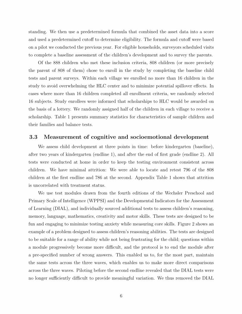
3.3 Measurement of cognitive and socioemotional development
We assess child development at three points in time: before kindergarten (baseline),
after two years of kindergarten (endline 1), and after the end of first grade (endline 2). All
tests were conducted at home in order to keep the testing environment consistent across
children. We have minimal attrition: We were able to locate and retest 796 of the 808
children at the first endline and 786 at the second. Appendix Table 1 shows that attrition
is uncorrelated with treatment status.
We use test modules drawn from the fourth editions of the Wechsler Preschool and
Primary Scale of Intelligence (WPPSI) and the Developmental Indicators for the Assessment
of Learning (DIAL), and individually sourced additional tests to assess children’s reasoning,
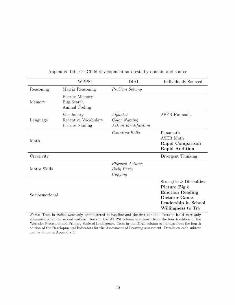
memory, language, mathematics, creativity and motor skills. These tests are designed to be
fun and engaging to minimize testing anxiety while measuring core skills. Figure 2 shows an
example of a problem designed to assess children’s reasoning abilities. The tests are designed
to be suitable for a range of ability while not being frustrating for the child; questions within
a module progressively become more difficult, and the protocol is to end the module after
a pre-specified number of wrong answers. This enabled us to, for the most part, maintain
the same tests across the three waves, which enables us to make more direct comparisons
across the three waves. Piloting before the second endline revealed that the DIAL tests were
no longer sufficiently difficult to provide meaningful variation. We thus removed the DIAL
6

instruments and added two new math assessments to maintain coverage of most domains for
the second endline.
Directly assessing children’s socioemotional development at these ages and in the field
is challenging without highly trained evaluators. For the first endline, we rely on parents’
reports by administering the widely used Strengths and Difficulties Questionnaire or SDQ.
This questionnaire asks parents to rate whether several statements about their child (such
as “Restless, overactive, cannot stay still for long”) are “not true”, “somewhat true” or
“certainly true”. At the second endline, when children are older, we adapted or created
ways to directly assess children’s motivation to learn, personalities, ability to read others’
emotions, prosociality, and behavioral performance in school. Appendix Table 2 summarizes
all of the measures administered to the children and Appendix C provides the details of each
measure.
4 Estimation strategy
4.1 Effects of being offered a scholarship and of attending HLC
We pre-specified two primary specifications, a reduced-form model and an instrumental
variables (IV) model. The reduced-form model of the effect of the scholarship offer, which
we estimate separately for each endline wave, is as follows:
yij = β1scholarshipij + β2y0ij + villagej + f(genderij, ageij) + εij (1)
where yij is an outcome for child i in village j, scholarshipij is whether the child was offered
a scholarship, y0ij is the baseline value of yij if available, villagej are fixed effects for the
villages, and f(genderij, ageij) are age and gender controls. Specifically, we pre-specified
that if neither age and gender fixed effects nor an age cubic-polynomial interacted with
gender improved explanatory power in the control group at endline, that we would use a
non-interacted cubic polynomial in age with an indicator for gender for this set of controls.
Based on this algorithm, we use the non-interacted controls throughout.
We also estimate the following IV model, which pools across different counterfactual
options:
yij = β1enrolled in HLCij + β2y0ij + villagej + f(genderij, ageij) + εij (2)
7

where being enrolled in HLC is now instrumented with the scholarship offer. We use enroll-
ment in HLC as the endogenous variable rather than enrollment in kindergarten because the
scholarship increased not only the likelihood of attending kindergarten but also which kinder-
garten a child attended. In other words, treatment induced some children to switch from
attending another kindergarten to attending HLC, which would be an exclusion restriction
violation if “enrolled in kindergarten” were the endogenous variable.6
One potential concern with this IV model is that the scholarship also reduces the fees
paid by always takers and those who switch to HLC from another kindergarten. Thus, income
could be another channel besides HLC attendance that is affecting test scores. Parental
spending on educational inputs like books is negligible in our setting and we do not find any
effect of treatment on such spending. A back of the envelope calculation suggests that an
income effect operating through other channels such as nutrition is very unlikely to produce
the large impacts on cognition we find.
Our outcomes are z-score indices. For each test, we subtract off the control mean and
divide by the standard deviation.7 We then average across all cognitive tests to form our
primary outcome, within the domains shown in Table 2 to form domain-specific indices, and
across the socioemotional measures.
4.2 Decomposing the effect by counterfactual activity
Our compliers – children who attend HLC because of the scholarship – are a het-
erogeneous group who vary in what they would have done absent the scholarship. The
LATE estimated using the pooled IV above is a weighted average of these counterfactual-
specific LATEs or “subLATEs.”. In this section, we describe how we separately estimate the
counterfactual-specific effects.
We focus on a specific dimension of the fallback heterogeneity – the child’s propensity to
enroll in a kindergarten absent the scholarship. Understanding how these effects differ is not
only intellectually interesting, but also policy relevant. Consider a government contemplating
expanding a voucher program similar to the scholarships that we randomize. The effect
6We deviate here from our pre-analysis plan, which stated we would use “enrolled in any kindergarten” asthe endogenous variable. We realized the extent of the exclusion restriction violation was non-trivial whenwe saw that a large share of children induced to attend HLC switch from other kindergarten providers.
7Before the first endline, we specified that we would use the baseline control mean and standard deviationfor this normalization. We realized that that choice makes it more difficult to make direct comparisons acrosswaves, as test composition and the standard deviations change. Therefore before endline 2 we pre-specifiedthat we would use contemporaneous control group values.
8

of our scholarship on children who otherwise would not have attended kindergarten gives
insight into how large of an effect the government might expect if it could perfectly target
the program towards families who would otherwise not send their children to kindergarten.
In addition, the impact on switchers from other kindergartens is informative about about
whether our provider is better or worse than other providers in the market. This relative
position is important for deciding how restricted the vouchers should be across providers.
By dividing counterfactual activity into two categories, we are pooling together children
who would have stayed home with those who would have attended anganwadi centers.8 We
would ideally have liked to separately identify these effects, but we have very few children
who stay at home so too little power to do so. Similarly, some children have a mixture of two
activities, such as one year of anganwadi and then one year of another kindergarten. Again for
statistical power reasons, we ignore these subtleties. We believe the dichotomous approach
captures the most important aspect of the heterogeneity, whether a child is receiving a formal
school curriculum or not.
One approach to measuring counterfactuals that we used was simply to ask parents.
Unlike many studies on kindergarten or pre-K, ours is prospective, so we asked parents at
baseline what their plans were if they did not receive the scholarship. Appendix Table 3
shows the predictive power of these baseline reports on ultimate enrollment decisions for the
control group. Unfortunately, these plans are less predictive than might be hoped, possibly
because parents thought we would use the information to assign scholarships, even when we
truthfully explained we would not, or because these decisions are last-minute.
We improve on this by following Crepon et al. (2019) in using machine learning (ML)
to predict counterfactual probabilities that the child will be enrolled in kindergarten using
covariates (including the baseline survey responses about enrollment plans). We proceed as
follows:
1. For each village, we fit a LASSO model using repeated cross validation on the other
70 villages to predict years of kindergarten and treatment status.
2. Using predictors selected by LASSO, we then run OLS and logit respectively to remove
LASSO bias. We then use these estimations to form predictions for individuals in the
selected village.
8We predict years of any kindergarten attended, which pools those who would have attended HLC andthose who would have attended another kindergarten absent the scholarship. The IV effect, however, isidentified off those who would have attended another kindergarten, for the usual reason that IV effects arenot identified off of always takers.
9

3. We repeat this 1000 times and take the median of the 1000 predictions to purge any
estimation variability. Appendix Figure 1 shows this procedure appears to successfully
result in fully converged values.
4. Finally, we residualize treatment with its predicted value and estimate the regression
with the weights from Crepon et al. (2019) to orthogonalize the final estimate with
regard to machine learning prediction error.
With the ML prediction in hand, we can then examine how the treatment effect varies
with the predicted years of attending kindergarten absent the scholarship. If we are willing to
make additional assumptions, the method in Hull (2018) allows us to obtain point estimates
for two different types of compliers. Specifically, we can use the ML prediction to construct
a second instrumental variable by interacting the treatment indicator, scholarshipij, with
the predicted years of attending kindergarten, KGyearsij.
We use the two instruments in an IV estimation with two endogenous regressors that
represent mutually exclusive and collectively exhaustive counterfactuals for the compliers.
Specifically, we define the two counterfactuals as always attended anganwadi or home care
and ever attended a non-HLC kindergarten. (The variables are defined with the qualifiers
‘always’ and ‘ever’ because some children engage in different activities across the two years.)
We expect the instruments to reduce these endogenous regressors, with children shifting
away from these activities toward HLC.9 The IV coefficient on the ‘always anganwadi/home’
endogenous regressor represents the effect of attending HLC for a child who would have
otherwise always attended anganwadi/home. The second IV coefficient is the effect for a
child induced to attend HLC who would have otherwise attended another kindergarten (for
either one or two years).
The additional assumptions we make in estimating with this two-instrument model are
as follows: 1) There are two, exclusive types of compliers (those that ever go to kindergarten
and those that do not without the scholarship), and 2) the subLATEs for these compliers are
mean independent of our prediction of their propensity to attend kindergarten. That is, the
heterogeneity of the reduced-form effects by the predicted counterfactual is due just to this
variable shifting the counterfactual, not to, say, affecting how much of the HLC curriculum
a student absorbs. While this second assumption is obviously restrictive, we believe this still
adds useful information above and beyond the overall IV results.
9The residual category of attending HLC is, specifically, “always attended HLC or attended a combinationof HLC and home/anganwadi.
10

5 Results at the end of kindergarten
5.1 Enrollment in kindergarten
We now turn to presenting our empirical results. Figure 3 breaks down children’s
enrollment status, separately for the treatment and control groups and for the first and second
years of the kindergarten period. In the control in the first year, 54% of children attend the
anganwadi and another 5% are cared for at home. Most of the others attend kindergarten
(17% at HLC and 23% at another KG). In the treatment group, the share at HLC increases
by 51 percentage points to 68%. Few students attend a different kindergarten than HLC, but
surprisingly, 25% of children attend anganwadis. That is, the take-up rate of the scholarship
among would-be anganwadi attendees is about a half. Some factors are that anganwadi
workers often (incorrectly) told parents they would lose eligibility for various government
programs if they did not send their child to the anganwadi; some parents perceived the
quality or convenience of the anganwadi as higher than HLC; or the 1000 rupee co-pay was
too costly.
The effect on attending HLC is smaller in the second year. This is because enrollment
in other kindergartens is much higher in the second year. The decision to enroll children in
just upper kindergarten could be because some families can only afford one year of fees. In
addition, often families who wish to send their children to a specific private primary school
enroll their child in that school’s kindergarten in the year before first grade to secure a
slot. In the treatment group, some children switch from HLC to another kindergarten in the
second year. This could be for the same reason (during our study period, HLC specialized
only in kindergarten), or it is also possible some parents were dissatisfied with HLC.10
Table 2 shows the regression results for enrollment. The scholarship offer increases the
likelihood of attending HLC by 47 percentage points and the likelihood of attending any
kindergarten by around 20 percentage points. Thus, the compliers are split roughly evenly
between those who would have not attended kindergarten without the scholarship and those
who switch from other kindergartens.
5.2 Effects on child development
We next turn to the impacts on the index of cognitive test scores. Table 3, column
3, shows being offered a scholarship increases performance on our total score index by 0.4
10Appendix Table 4 shows the full transition matrix between year 1 and year 2.
11

standard deviations. As seen from the cumulative distributions of test scores for the treat-
ment and control group presented in Figure 4, the treatment effect is spread throughout the
achievement distribution. The treatment group’s score distribution first order stochastically
dominates the control group’s.
These gains are also widely spread across skill domains. Table 4 shows that the IV
effect of attending HLC ranges from 0.33 to 0.97 standard deviations across domains. While
it is tempting to interpret the relative size of these domain improvements as evidence for
which areas HLC is more or less skilled at teaching, it is important to remember that there
are likely different elasticities of knowledge to inputs across these domains. For example,
one can very directly improve mathematics performance by teaching children numbers. In
contrast, improving reasoning skills requires a much more indirect approach. In addition,
the effect sizes also reflect how well these skills are taught via the counterfactual activity,
e.g., at the anganwadi center or at other kindergartens.
In contrast to these large improvements, we find no improvement on either the aggregate
socioemotional index nor on the subdomains of the questionnaire. The last column of Table 4
shows that not only is the effect insignificant, but the point estimate is also small. One
explanation for this null result is that parental reports are not a good way to measure
children’s socioemotional development. This concern led us to add more direct assessments
of children to endline 2, when the children were older.11
5.3 Counterfactual-specific effects
Accuracy of predictions
The prediction method outlined in subsection 4.2 appears to yield fairly accurate pre-
dictions. Appendix Figure 2 shows a binscatter of the true enrollment decisions against the
ones predicted by the procedure. Recall that because these predictions were formed based
on the other villages, we can think of this scatter plot as showing out-of-sample performance.
It achieves this fit using a variety of predictors summarized in Table 5.
Table 6 shows how the first stage effects of the scholarship differ by the predicted
propensity to attend kindergarten without a scholarship. The first two columns show that
the effect of the scholarship on inducing children to enroll in HLC is similar for those above
and below the median of Predicted Years of Kindergarten. This pattern is in line with the
first stage results shown in Table 2, which indicated a roughly equal split of compliers coming
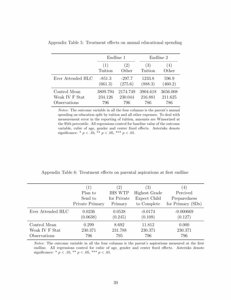
11Appendix Tables 5 to 10 report other analyses laid out in our pre-analysis plan.
12

from non-kindergarten (mostly anganwadis) and other private kindergartens.
In next two columns of Table 6, the outcome variables are the two mutually exclu-
sive counterfactual options of always having home care or attending anganwadi and ever
attending a non-HLC kindergarten. While columns 1 and 2 showed that Predicted Years of
Kindergarten does not predict enrolling in HLC as a result of being offered the scholarship,
it does predict which fallback option students are drawn from. The main effect of Predicted
Years of Kindergarten verifies that the prediction is informative in the control group. As
expected, the predicted value is negatively correlated with attending anganwadi/home and
positively correlated with attending another kindergarten.
The main effect of Treatment gives the effect of the scholarship for those predicted to
not attend kindergarten. The scholarship reduces the likelihood that these children attend
anganwadi/home (column 4), and reassuringly, has no effect on their attendance at other
kindergartens, which was predicted to be zero anyway. Finally, the interaction effects gives
the additional effect of the scholarship per predicted year of kindergarten. In column 3,
we expect the interaction to be the opposite sign and half the magnitude of the coefficient
on Treatment, because the scholarship should not affect attending anganwadi/home for
those predicted to attend two years of kindergarten. The ratio of the coefficients lines
up closely with this pattern. Finally, the magnitude of the interaction effect in column
4 should be negative and smaller in magnitude than the coefficient on Predicted Years of
Kindergarten. While the interaction coefficient is negative, its magnitude is in fact larger
than if the prediction were perfect.
Effect of scholarship for switchers from no kindergarten and other kindergartens
We next incorporate the predicted counterfactual enrollment in kindergarten into the
treatment effect estimates on test scores. We find that while all students benefit from the
scholarship offer, those who switched from not going to kindergarten experience the largest
gains at the first endline.
The first two columns of Table 7 show the IV effect of enrolling at HLC estimated for
those both above versus below the median of propensity to enroll in kindergarten. There is
clear evidence of treatment effect heterogeneity, as the effect for compliers with below median
propensity to attend kindergarten is significantly larger than the effect on those above the
median.
The third column of Table 7 shows the IV estimate of attending HLC separately for
13

the two counterfactuals. The differences are stark. The local average treatment effect for
compliers who switch from anganwadi or home is 1.4 standard deviations, or over three times
as large as that estimate for compliers switching from other kindergartens. These two effects
are statistically different from each other. This large gap is not because there is a small effect
for those switching from other kindergartens. We estimate that those students still improve
performance on our tests by more than 0.4 standard deviations.
6 Results at the end of first grade
6.1 Primary school enrollment
We find no effects on primary school enrollment. The last two columns of Table 2
show children who received the scholarship are neither more likely to attend primary school
at the age-appropriate time nor more likely to be enrolled in a private primary school.
This simplifies the interpretation of the second endline results because the only differences
in education induced by the scholarship are the pre-primary decisions and not subsequent
enrollment. Additionally, it is interesting that parents appear to neither be complementing
the educational investment induced by the scholarship nor substituting resources away.
6.2 Effects on child development
While diminished, the effect of attending HLC remain statistically and economically
significant. Table 8 shows that those who were induced into attending HLC by the scholarship
score 0.4 SD better than their peers at the end of first grade. With the exception of the far
left tail, the treatment group continues to dominate the control group’s score as shown in
Figure 5, and the gains are seen broadly across skill domains (Table 9).
To understand the rate at which the effects diminish, a simple comparison of the esti-
mated effects at the first and second endlines is not quite correct because the test composition
changed between the two waves and because the effects are standardized differently. Thus,
we also create a common benchmark by first restricting to the set of tests common across
all three survey waves, and then generating new averages of z-scores that are standardized
using the control group at the first endline. Using this new index, Table 10 shows that
approximately 40% of the effect persists from endline 1 to endline 2.12
12A natural follow-up question is whether the effect is diminishing because treatment students are learningat a slow rate or the control students are learning at a faster pace. Appendix Figure 3 gives some sense of theanswer by plotting the raw versions of these common scores over time. Taking the cardinal interpretation
14
Interestingly, we continue to find no evidence of improved socioemotional skills on any of
the direct assessment measures we use or an index that combines them. As shown in Table 11,
we find no effect on children’s contentiousness, willingness to attempt hard problems, their
willingness to share with another child, or other measures. One explanation for the lack of
effect is that very few students in the control group are cared for exclusively at home. Thus,
even those not enrolled in kindergarten experience a similar social environment. Anganwadi
centers are similarly sized, with children of similar ages.
6.3 Counterfactual-specific effects
At the second endline, we no longer find a large difference in the treatment effect size by
the child’s predicted likelihood of attending kindergarten without the scholarship. Columns
4 and 5 of Table 7 show the pooled IV estimates for those above and below the median
propensity to enroll in kindergarten. The estimated effects still differ, but no longer signifi-
cantly so. The counterfactual-specific IV estimates show even less evidence of heterogeneity
with almost identical point estimates. This suggests that one reason for the convergence in
scores may be that children who were not in kindergarten mostly catch up on the basics
such as knowing their numbers and alphabet that they missed out on by not being in kinder-
garten, leaving only the relative advantage of HLC over other kindergartens as the persistent
component.
7 Conclusion
As governments around the world begin to expand access to early childhood education,
there are many choices they face. They must decide whether it should be provided publicly
or by the private market, how much to subsidize the costs, how it should be financed, and
how formal the instruction should be.
In this study, we estimate the effects of providing subsidies to attend private, formal
kindergarten. The alternative for much of our sample is a government-run play-based com-
munity center. We find that attending a more formal learning environment has large and
enduring effects on children’s cognitive outcomes. Immediately after kindergarten, those
induced into attending formal kindergarten have roughly doubled the rate of learning com-
pared to the peers who did not attend kindergarten. We find that the effects are concentrated
of the score literally, it appears that treatment is on a relatively constant upward trend, while the controlgroup shows a sharp increase in the rate of growth between the first and second endlines.
15

mainly among those who would not have attended kindergarten, but that there are still ben-
efits to those who switch from other kindergarten providers. We also find that one year after
the intervention, an economically important portion of this improvement persists.
In contrast, we consistently fail to find improvements in socioemotional skills. This
is likely because while kindergarten has a more rigorous pedagogical approach than the
counterfactual but does not greatly change the extent of social interaction. Children in
both kindergartens and anganwadi centers are organized in groups and supervised by similar
authority figures. To investigate this hypothesis further it would be useful to be able to
identify the effects of our scholarship on children whose counterfactual is home care. In
principle, this could be done with the same machine learning approach that we use, but
unfortunately too small a proportion chooses home care to make this a fruitful strategy
using our sample.
In summary, if the goal of early childhood education is to improve cognitive outcomes,
there appear to be substantial benefits to investing in the infrastructure necessary to imple-
ment a more formal curriculum. Moreover, our implementing partner demonstrates that this
can be done at relatively large scale. However, if the goal is to foster socioemotional learning,
it appears unlikely that greater formality will yield additional gains beyond community day
care.
16

References
Almond, D. and J. Currie (2011). Human Capital Development before Age Five, Volume 4.
Elsevier B.V.
Andrew, A., O. Attanasio, R. Bernal, L. C. Sosa, S. Krutikova, and M. Rubio-Codina (2019).
Preschool Quality and Child Development. NBER Working Paper .
Attanasio, O., S. Cattan, E. Fitzsimons, C. Meghir, and M. Rubio-Codina (2015). Estimating
the Production Function For Human Capotal: Results From a Randomized Control Trail
in Colombia.
Belur, R. (2019, may). Kindergarten classes at govt schools from this year.
Berkes, J. and A. Bougen (2019). Heterogeneous Preschool Impact and Close Substitutes:
Evidence from a Preschool Construction Program in Cambodia. Mimeo.
Blimpo, M. P. and T. Pugatch (2017). Scaling up Children’s School Readiness in The
Gambia: Lessons from an Experimental Study. Mimeo.
Bouguen, A., D. Filmer, K. Macours, and S. Naudeau (2018). Preschool and Parental
Response in a Second Best World: Evidence from a School Construction Experiment.
Journal of Human Resources 53 (2), 474–512.
Crepon, B., E. Duflo, E. Huillery, W. Pariente, J. Seban, and P.-A. Veillon (2019). Cream
skimming and the comparison between social interventions: Evidence from entrepreneur-
ship programs for at-risk youth in France. Mimeo.
Duflo, E., P. Dupas, and M. Kremer (2011). Peer effects, teacher incentives, and the im-
pact of tracking: Evidence from a randomized evaluation in Kenya. American Economic
Review 101 (5), 1739–1774.
Engle, P. L., L. C. Fernald, H. Alderman, J. Behrman, C. O’Gara, A. Yousafzai, M. C.
De Mello, M. Hidrobo, N. Ulkuer, I. Ertem, and S. Iltus (2011). Strategies for reducing
inequalities and improving developmental outcomes for young children in low-income and
middle-income countries. The Lancet 378 (9799), 1339–1353.
Gertler, P., J. Heckman, R. Pinto, A. Zanolini, C. Vermeersch, S. Walker, S. M. Chang, and
S. Grantham-McGregor (2014). Labor Market Returns to an Early Childhood Stimulation
Intervention in Jamaica. Science 344 (6187), 998–1001.
17
Glewwe, P., M. Kremer, and S. Moulin (2009). Many children left behind? textbooks and
test scores in kenya. American Economic Journal: Applied Economics 1 (1), 112–35.
Heckman, J. J., S. H. Moon, R. Pinto, P. A. Savelyev, and A. Yavitz (2010). The rate of
return to the HighScope Perry Preschool Program. Journal of Public Economics 94 (1-2),
114–128.
Hull, P. (2018). IsoLATEing: Identifying Counterfactual-Specific Treatment Effects with
Cross-Stratum Comparisons. Mimeo.
Imbens, G. W. and D. B. Rubin (2015). Causal inference in statistics, social, and biomedical
sciences. Cambridge: Cambridge University Press.
Jebaraj, P. (2019, jun). Draft National Education Policy proposes formal education from
age of three.
Kline, P. and C. R. Walters (2016). Evaluating public programs with close substitutes: The
case of Head Start. The Quarterly Journal of Economics 131 (4), 1795–1848.
Kosse, F., T. Deckers, P. Pinger, H. Schildberg-Hoerisch, and A. Falk (2019). The Formation
of Prosociality: Causal Evidence on the Role of Social Environment. Journal of Political
Economy .
LoBue, V. and C. Thrasher (2015). The child affective facial expression (cafe) set: validity
and reliability from untrained adults. Frontiers in Psychology 5, 1532.
Mackiewicz, M. and J. Cieciuch (2016). Pictorial Personality Traits Questionnaire for Chil-
dren (PPTQ-C)-a new measure of children’s personality traits. Frontiers in Psychol-
ogy 7 (498).
Martinez, S., S. Naudeau, and V. Pereira (2017). Preschool and Child Development un-
der Extreme Poverty Evidence from a Randomized Experiment in Rural Mozambique.
Mimeo (December).
Muralidharan, K., A. Singh, and A. J. Ganimian (2019). Disrupting education? Experimen-
tal evidence on technology-aided instruction in India. American Economic Review 109 (4),
1426–1460.
18

Table 1: Balance test of baseline characteristics for treatment and control groups
Treatment Control P-valuesNormalizedDifferences
Child Demographics
Age (Years) 3.975 3.995 0.503 -0.047
Female 0.483 0.493 0.779 -0.020
Child Test Scores
Total Score -0.034 -0.000 0.646 -0.032
Reasoning -0.028 0.000 0.699 -0.027
Memory 0.031 0.000 0.691 0.029
Language -0.038 -0.000 0.607 -0.038
Math -0.158 -0.000 0.037 -0.165
Motor Skills -0.027 -0.000 0.738 -0.027
Guardian Demographics
Asset Index 0.038 -0.000 0.583 0.039
Male Education (Years) 6.739 7.212 0.098 -0.118
Female Education (Years) 7.145 7.193 0.853 -0.013
Number of children 404 404
Joint p-value: 0.451Multivariate Normalized Difference: 0.252
Notes: P-values in columns are for a test of equality between the control and treatment means. Thenormalized difference is the difference between the treatment mean and the control mean divided by thesquare root of the average variance of the sample. The joint p-value is for a test of joint equality of alllisted control and treatment means. The multivariate normalized difference is computed as in Imbensand Rubin (2015).
19

Table 2: First stage results
(1) (2) (3) (4) (5) (6) (7) (8)Ever Attended
KGEver Attended
HLCYears Attended
HLCEver Attended
Other KGEver
Home CareEver Attended
AnganwadiAttend Any
PrimaryAttend Private
Primary
Treatment 0.196∗∗∗ 0.467∗∗∗ 0.948∗∗∗ -0.286∗∗∗ -0.0384∗∗ -0.303∗∗∗ 0.0263 -0.0189(0.0304) (0.0308) (0.0552) (0.0288) (0.0195) (0.0323) (0.0162) (0.0315)
Control Mean 0.601 0.226 0.329 0.437 0.101 0.585 0.934 0.327Observations 796 796 796 796 796 796 783 783
Notes: All columns control for a cubic of age, gender, and center fixed effects. Asterisks denote significance: * p < .10, ** p < .05, *** p < .01.
20

Table 3: Treatment effects on total score at first endline
(1) (2) (3) (4) (5)OLS OLS RF IV IV
Ever Attended HLC 0.411∗∗∗ 0.556∗∗∗ 0.835∗∗∗
(0.125) (0.119) (0.110)
Ever Attended Other 0.402∗∗∗
KG (0.108)
Ever Attended -0.493∗∗∗
Anganwadi (0.110)
Treatment 0.392∗∗∗
(0.0609)
Years Attended HLC 0.412∗∗∗
(0.0538)
Control Mean 0.000 0.000 0.000 0.000 0.000Weak IV F Stat 236.145 302.999Observations 397 397 796 796 796
Notes: The outcome variable in all the four columns is the child’s endline totalscore. The total score is calculated by normalizing various sub-tests with respectto the control, averaging the standardized values, and then re-standardizing tothe control. All regressions control for baseline test score, cubic of age, genderand center fixed effects. To avoid including the effect of the scholarship, theOLS columns are restricted to the control group. Asterisks denote significance: *p < .10, ** p < .05, *** p < .01.
21

Table 4: IV effects by test domain at first endline
(1) (2) (3) (4) (5) (6) (7)Reasoning Memory Language Math Creativity Motor SEL
Ever Attended HLC 0.371∗∗∗ 0.553∗∗∗ 0.889∗∗∗ 0.968∗∗∗ 0.323∗∗ 0.433∗∗∗ -0.0407(0.134) (0.123) (0.113) (0.131) (0.137) (0.122) (0.140)
Control Mean -0.000 -0.000 -0.000 0.000 -0.000 -0.000 -0.000Weak IV F Stat 232.258 231.075 234.292 237.877 222.158 240.026 230.371Observations 796 796 796 796 782 796 796
Notes: The outcome variables in all the columns are standardized values of the respective test domain.The total score is calculated by normalizing various sub-tests within each test domain with respect to thecontrol, averaging the standardized values, and then re-standardizing to the control. All regressions controlfor baseline test score, cubic of age, gender and center fixed effects. Asterisks denote significance: * p < .10,** p < .05, *** p < .01.
22

Table 5: Predictors of kindergarten enrollment selected by LASSO
Variable Chosen Percentage of Time Chosen
Asset Test 100.00%Total Baseline Test Score 100.00%Spending on Older Sibling’s KG 99.92%Female Guardian Education 99.87%Age of Mother at First Birth 99.85%Older Sibling Did Not Go to KG 98.34%Average Number of Children per HH (Census) 98.05%Travel Time to HLC 97.99%Perceived Anganwadi Caretaker Quality 96.03%Child is Female 95.32%Number of Private KG in Village 84.63%Number of Private KG in Village in Past 75.44%Minimum You Should Pay for KG 31.87%Baseline Picture Memory Score 5.20%Baseline Bug Search Score 1.87%Most You Should Pay for KG 1.58%Parent Time Working Away from Home 1.53%Unemployment Rate (Census) 0.89%Perceived Other KG Facility Quality 0.36%Percentage Scheduled Caste Women (Census) 0.23%Percentage Scheduled Caste Men (Census) 0.20%Perceived Anganwadi Facility Quality 0.07%Percentage Scheduled Caste (Census) 0.06%Baseline Vocabulary Score 0.03%
Notes: Items appear in this table if any form of this variable (e.g. square, levels, indica-tors for levels of ordinal variables) are selected by LASSO. Percentages of time chosen byLASSO are computed weighting each of the 1000 iterations and each of the 71 villagesequally. Variables never chosen are omitted for space.
23

Table 6: First stage incorporating Predicted Years of Kindergarten
(1) (2) (3) (4)Attend HLC
(Below Median)Attend HLC
(Above Median)Always Home Care
or AnganwadiEver Attended
Other KG
Treatment 0.507∗∗∗ 0.475∗∗∗ -0.413∗∗∗ 0.0163(0.0438) (0.0462) (0.0711) (0.0640)
Treatment × 0.227∗∗∗ -0.314∗∗∗
Predicted Years KG (0.0610) (0.0623)
Predicted Years KG -0.222∗∗∗ 0.142∗∗∗
(0.0419) (0.0376)
Control Mean 0.161 0.288 0.399 0.437Observations 396 400 796 796
Notes: Asterisks denote significance: * p < .10, ** p < .05, *** p < .01.
24

Table 7: Heterogeneity of effects on total score by Predicted Years of Kindergarten & counterfactual-specific treatment effects
Endline 1 Endline 2
(1) (2) (3) (4) (5) (6)
Below Median Above MedianCounterfactual-specific LATE
Below Median Above MedianCounterfactual-specific LATE
Ever Attended HLC 1.037∗∗∗ 0.604∗∗∗ 0.562∗∗∗ 0.279(0.149) (0.148) (0.175) (0.187)
Always Angan. Fallback 1.355∗∗∗ 0.370(0.296) (0.408)
Ever Other KG Fallback 0.438∗∗ 0.465(0.186) (0.301)
Control Mean -0.396 0.375 0.000 -0.295 0.283 0.000Equal Effects P-Value 0.029 0.035 0.244 0.885KP F-Stat 134.206 105.837 12.009 122.153 99.598 8.936Observations 396 400 796 394 387 781
Notes: Asterisks denote significance: * p < .10, ** p < .05, *** p < .01.
25

Table 8: Treatment effects on total score at second endline
(1) (2) (3) (4) (5)OLS OLS RF IV IV
Ever Attended HLC 0.339∗∗ 0.327∗∗ 0.427∗∗∗
(0.141) (0.132) (0.135)
Ever Attended Other 0.470∗∗∗
KG (0.136)
Ever Attended -0.218∗
Anganwadi (0.131)
Treatment 0.196∗∗∗
(0.0669)
Years Attended HLC 0.210∗∗∗
(0.0664)
Control Mean 0.000 0.000 0.000 0.000 0.000Weak IV F Stat 217.409 281.435Observations 390 390 786 786 786
Notes: The outcome variable in all the four columns is the child’s endline totalscore. The total score is calculated by normalizing various sub-tests with respectto the control, averaging the standardized values, and then re-standardizing to thecontrol. All regressions control for baseline test score, cubic of age, gender and centerfixed effects. To avoid including the effect of the scholarship, the OLS columns arerestricted to the control group. Asterisks denote significance: * p < .10, ** p < .05,*** p < .01.
26

Table 9: Treatment effects by test domain at second endline
(1) (2) (3) (4) (5) (6)Reasoning Memory Language Math Creativity SEL
Ever Attended HLC 0.235 0.229 0.345∗∗ 0.409∗∗∗ 0.273∗ 0.0682(0.144) (0.143) (0.138) (0.141) (0.146) (0.139)
Control Mean -0.000 -0.000 0.000 0.000 -0.000 -0.000Weak IV F Stat 215.152 213.306 215.095 217.928 195.684 213.634Observations 786 786 786 786 755 786
Notes: The outcome variables in all the columns are standardized values of the respective test domain.The total score is calculated by normalizing various sub-tests within each test domain with respect tothe control, averaging the standardized values, and then re-standardizing to the control. All regressionscontrol for baseline test score, cubic of age, gender and center fixed effects. Asterisks denote significance:* p < .10, ** p < .05, *** p < .01.
27

Table 10: Treatment effects on tests common across endlines
(1) (2)Endline 1 Endline 2
Ever Attended HLC 0.900∗∗∗ 0.379∗∗∗
(0.118) (0.120)
Control Mean -0.000 1.191Weak IV F Stat 239.283 219.605Observations 796 786
Notes: The outcome variables in all the columnsare standardized values of the tests common acrossboth endlines. The individual measure outcomesare calculated by standardizing measure with re-spect to the first endline control. The total indexis an average of these z-scores which is then re-standardized with respect to first endline control.All regressions control for baseline test score, cubicof age, gender and center fixed effects. Asterisksdenote significance: * p < .10, ** p < .05, ***p < .01.
28

Table 11: IV effects by socioemotional domain at second endline
(1) (2) (3) (4) (5) (6)
Total Index Prosociality ConscientiousEmotionDetection
MotivationLeadership
Position
Ever Attended HLC 0.0682 -0.0129 -0.0460 -0.0764 0.109 0.206(0.139) (0.142) (0.150) (0.146) (0.146) (0.140)
Control Mean -0.000 -0.000 0.000 0.000 -0.000 -0.000Weak IV F Stat 213.634 213.634 213.634 213.634 213.203 212.365Observations 786 786 786 786 778 783
Notes: The outcome variables in all the columns are standardized values of the SEL measures. The individualmeasure outcomes are calculated by standardizing each SEL measures with respect to the control. The totalindex is an average of these z-scores which is then re-standardized with respect to control. All regressions controlfor baseline test score, cubic of age, gender and center fixed effects. Asterisks denote significance: * p < .10, **p < .05, *** p < .01.
29

Figure 1: Study villages
Notes: This map shows the locations of the study villages in dark blue and the ten districts of Karnatakain which the villages are located in light blue.
30

Figure 2: Example of reasoning assessment
Notes: This measure assess children’s ability to use reasoning to complete patterns. They are shown aseries of boxes with a space missing and have to choose from among the available options which correctlycompletes the pattern. The test begins with very simple patterns and proceeds to become more difficultuntil children incorrectly answer three questions in a row. At no time are children given feedback on theirperformance.
31

Figure 3: Effect of scholarship on enrollment decisions
17%
23%
54%
5%
68%
4%
25%
15%
30%
38%
7%
10%
60%
10%
21%
4%5%
Year 1 Year 2
Control Treatment Control Treatment
0%
25%
50%
75%
100%
Per
cent
age
Cho
osin
g Sc
hool
ing
Opt
ion
Hippocampus Other KG Anganwadi
Stay Home Other
Notes: This figure shows the percentage of children choosing each enrollment option for each of the twopossible years of KG by treatment status.
32

Figure 4: Total score distributions at first endline
0.00
0.25
0.50
0.75
1.00
-2 0 2Total Score
Cum
ulat
ive
Den
sity
Control Treatment
Notes: This figure shows the CDFs of the total score variable for both the treatment and control groups atthe first endline. The scores of those that received a scholarship offer first order stochastically dominatethose of the control.
33

Figure 5: Total score distributions at second endline
0.00
0.25
0.50
0.75
1.00
-4 -2 0 2Total Score
Cum
ulat
ive
Den
sity
Control Treatment
Notes: This figure shows the CDFs of the total score variable for both the treatment and control groups atthe second endline. The scores of those that received a scholarship offer first order stochastically dominatethose of the control except at the left tail.
34

A Appendix Tables
Appendix Table 1: Test for attrition balance
(1) (2) (3)Endline 1 Endline 2 Ever
Treatment -0.00495 -0.0149 -0.0124(0.00852) (0.0115) (0.0127)
Control Mean 0.017 0.035 0.040Observations 808 808 808
Notes: Columns show whether an individual attrits in endline 1, endline 2, or ever respectively. Attrition levelsare low and uncorrelated with treatment status.
35
Appendix Table 2: Child development sub-tests by domain and source
WPPSI DIAL Individually Sourced
Reasoning Matrix Reasoning Problem Solving
MemoryPicture MemoryBug SearchAnimal Coding
LanguageVocabulary Alphabet ASER KannadaReceptive Vocabulary Color NamingPicture Naming Action Identification
Math
Counting Balls PanamathASER MathRapid ComparisonRapid Addition
Creativity Divergent Thinking
Motor SkillsPhysical ActionsBody PartsCopying
Socioemotional
Strengths & DifficultiesPicture Big 5Emotion ReadingDictator GameLeadership in SchoolWillingness to Try
Notes: Tests in italics were only administered at baseline and the first endline. Tests in bold were onlyadministered at the second endline. Tests in the WPPSI column are drawn from the fourth edition of theWechsler Preschool and Primary Scale of Intelligence. Tests in the DIAL column are drawn from the fourthedition of the Developmental Indicators for the Assessment of Learning assessment. Details on each subtestcan be found in Appendix C.
36

Appendix Table 3: Accuracy of parents’ stated plans for enrollment
(1) (2) (3) (4) (5)Ever Attended
KGEver Attended
HLCEver Attended
Other KGEver
Home CareEver Attended
AnganwadiState Prefer KG in Control 0.127∗∗ 0.0803 0.0770 -0.00386 -0.210∗∗∗
(0.0568) (0.0502) (0.0534) (0.0375) (0.0552)Control Mean 0.601 0.226 0.437 0.101 0.585Observations 388 388 388 388 388
Notes: All columns control for a cubic of age, gender, and center fixed effects. Asterisks denote significance: * p < .10, **p < .05, *** p < .01.
37

Appendix Table 4: Transition matrix for enrollment across the two years of kindergarten
Year 2HLC Other KG Angan. Other
Year 1
HLC 276 26 29 12Other KG 7 74 9 16Angan. 17 60 238 28Other 0 1 1 3
Notes: The table displays the frequency counts of children basedon their first year kindergarten enrollment decisions shown bythe rows and their second year enrollment decisions shown by thecolumns.
38
Appendix Table 5: Treatment effects on annual educational spending
Endline 1 Endline 2
(1) (2) (3) (4)Tuition Other Tuition Other
Ever Attended HLC -851.3 -297.7 1233.8 596.9(661.3) (275.6) (888.3) (460.2)
Control Mean 3809.794 2174.749 3904.618 3656.008Weak IV F Stat 234.126 230.044 216.881 211.625Observations 796 796 786 786
Notes: The outcome variable in all the four columns is the parent’s annualspending on education split by tuition and all other expenses. To deal withmeasurement error in the reporting of tuition, amounts are Winsorized atthe 95th percentile. All regressions control for baseline value of the outcomevariable, cubic of age, gender and center fixed effects. Asterisks denotesignificance: * p < .10, ** p < .05, *** p < .01.
Appendix Table 6: Treatment effects on parental aspirations at first endline
(1) (2) (3) (4)Plan toSend to
Private Primary
IHS WTPfor PrivatePrimary
Highest GradeExpect Childto Complete
PercivedPreparedness
for Primary (SDs)
Ever Attended HLC 0.0236 0.0538 -0.0174 -0.000669(0.0638) (0.245) (0.109) (0.127)
Control Mean 0.299 8.692 11.812 0.000Weak IV F Stat 230.371 231.788 230.371 230.371Observations 796 795 796 796
Notes: The outcome variable in all the four columns is the parent’s aspirations measured at the firstendline. All regressions control for cubic of age, gender and center fixed effects. Asterisks denotesignificance: * p < .10, ** p < .05, *** p < .01.
39

Appendix Table 7: First stage heterogeneity at first endline
(1) (2) (3) (4) (5) (6)EverHLC
EverHLC
EverHLC
EverHLC
EverHLC
EverHLC
Treatment 0.439∗∗∗ 0.470∗∗∗ 0.470∗∗∗ 0.466∗∗∗ 0.498∗∗∗ 0.432∗∗∗
(0.0452) (0.0306) (0.0305) (0.0308) (0.0710) (0.0631)
Treatment × 0.0598Female (0.0645)
Treatment × 0.0130Total Endowment (0.0424)
Treatment × 0.0459Baseline Total Score (0.0306)
Treatment × 0.00508Baseline Assets (0.0315)
Treatment × -0.00405Female Guardian Edu (0.00897)
Treatment × 0.00543Male Guardian Edu (0.00798)
Control Mean 0.226 0.226 0.226 0.226 0.226 0.226Observations 796 796 796 796 796 796
Notes: The outcome variable in all the four columns is an indicator for whether the child everenrolled at HLC. All regressions control for baseline value of the outcome variable, cubic of age,gender and center fixed effects. Asterisks denote significance: * p < .10, ** p < .05, *** p < .01.
40

Appendix Table 8: Treatment effect heterogeneity at first endline
(1) (2) (3) (4) (5) (6)Total Score Total Score Total Score Total Score Total Score Total Score
Ever Attended HLC 0.736∗∗∗ 0.861∗∗∗ 0.863∗∗∗ 0.844∗∗∗ 0.947∗∗∗ 0.837∗∗∗
(0.167) (0.108) (0.112) (0.110) (0.272) (0.241)
Ever Attended HLC 0.224× Female (0.239)
Ever Attended HLC -0.0747× Total Endowment (0.146)
Ever Attended HLC -0.142× Baseline Total Score (0.126)
Ever Attended HLC -0.156× Baseline Assets (0.108)
Ever Attended HLC -0.0140× Female Guardian Edu (0.0340)
Ever Attended HLC 0.00358× Male Guardian Edu (0.0282)
Weak IV F Stat 56.396 42.239 24.723 53.192 45.351 48.294Observations 796 796 796 796 796 796
Notes: The outcome variable in all the four columns is the child’s total score at the first endline. Allregressions control for baseline value of the outcome variable, cubic of age, gender and center fixed effects.Asterisks denote significance: * p < .10, ** p < .05, *** p < .01.
41

Appendix Table 9: First stage heterogeneity at second endline
(1) (2) (3) (4) (5) (6)EverHLC
EverHLC
EverHLC
EverHLC
EverHLC
EverHLC
Treatment 0.385∗∗∗ 0.459∗∗∗ 0.459∗∗∗ 0.455∗∗∗ 0.496∗∗∗ 0.420∗∗∗
(0.0479) (0.0310) (0.0311) (0.0312) (0.0732) (0.0644)
Treatment × 0.141∗∗
Female (0.0657)
Treatment × 0.0107Total Endowment (0.0433)
Treatment × 0.0402Baseline Total Score (0.0309)
Treatment × 0.00457Baseline Assets (0.0319)
Treatment × -0.00529Female Guardian Edu (0.00922)
Treatment × 0.00574Male Guardian Edu (0.00816)
Control Mean 0.226 0.226 0.226 0.226 0.226 0.226Observations 786 786 786 786 786 786
Notes: The outcome variable in all the four columns is an indicator for whether the childever enrolled at HLC. All regressions control for baseline value of the outcome variable,cubic of age, gender and center fixed effects. Asterisks denote significance: * p < .10, **p < .05, *** p < .01.
42

Appendix Table 10: Treatment effect heterogeneity at second endline
(1) (2) (3) (4) (5) (6)Total Score Total Score Total Score Total Score Total Score Total Score
Ever Attended HLC 0.303 0.468∗∗∗ 0.453∗∗∗ 0.448∗∗∗ 0.430 0.384(0.235) (0.132) (0.135) (0.133) (0.300) (0.285)
Ever Attended HLC 0.267× Female (0.302)
Ever Attended HLC -0.0373× Total Endowment (0.178)
Ever Attended HLC 0.0107× Baseline Total Score (0.160)
Ever Attended HLC -0.114× Baseline Assets (0.138)
Ever Attended HLC 0.00208× Female Guardian Edu (0.0388)
Ever Attended HLC 0.0100× Male Guardian Edu (0.0333)
Weak IV F Stat 35.765 53.495 23.090 77.639 45.782 46.604Observations 786 786 786 786 786 786
Notes: The outcome variable in all the four columns is the child’s total score at the second endline. Allregressions control for baseline value of the outcome variable, cubic of age, gender and center fixed effects.Asterisks denote significance: * p < .10, ** p < .05, *** p < .01.
43
B Appendix Figures
Appendix Figure 1: Convergence of ML Predictions over iterations
0.00
0.05
0.10
0.15
0 250 500 750 1000Iteration
Abs
olut
e C
hang
e in
Pre
dict
ion
50th Percentile 75th Percentile 99th Percentile
Notes: This figure shows how the prediction of years of kindergarten changes over each iteration of theprocedure. To better understand the convergence, each line shows a different percentile of change at eachiteration. By the 1000th iteration, even the 99th percentile change is zero.
44

Appendix Figure 2: Binscatter of predicted versus actual years of kindergarten
0.5
11.
52
Act
ual Y
ears
of K
inde
rgar
ten
0 .5 1 1.5 2Predicted Years of Kindergarten
Notes: This figure shows a binscatter of the actual years of kindergarten against the years predicted by themachine learning procedure. Because each prediction is formed with models trained on the other villages,these predictions can be considered out-of-sample.
45

Appendix Figure 3: Raw scores on common tests over time
-1.5
-1.0
-0.5
0.0
0.5
1.0
1.5
2016 2017 2018 2019
Com
mon
Tes
ts S
core
(SD
s)
Control Treatment
Notes: This figure shows the raw score on a total index of tests common to all time points, after beingstandardized to the first endline control to facilitate comparison of effect sizes over time. The trendsappear to show treatment on a stable upward trajectory while control improves the rate of learning after2018 when they enter primary school.
46

C Measurement Instruments Appendix
C.1 Baseline and Endline 1 Measures
In order to assess children’s development during the baseline and first endline, we ad-
ministered the following sub-tests drawn from the Wechsler Preschool Primary Scale of Intel-
ligence (WPPSI), the Development Indicators for the Assessment of Learning (DIAL), and
other individual sources:
WPPSI Matrix Reasoning: A game where the children are presented with a series
of 3 pictures in a matrix and must choose the option that completes the pattern.
Stops after three wrong answers. (See Appendix Figure 4)
Appendix Figure 4: WPPSI Matrix Reasoning example
WPPSI Vocabulary: Children are read a word (e.g. dog) and asked to define it.
The test stops after three consecutive wrong answers.
WPPSI Receptive Vocabulary: Child selects a response option from a figure that
best represents the word the examiner reads aloud. The test stops after three
consecutive wrong answers. (See Appendix Figure 5)
WPPSI Picture Naming: The child names depicted objects. The test stops after
three consecutive wrong answers.
47

WPPSI Picture Memory: A child views a picture for a specified amount of time (3
seconds for Item 1-6, and 5 seconds for item 7-25) then selects from the options on
a response page. The test stops after three consecutive wrong answers.
WPPSI Bug Search: Within 120 seconds, the child selects as many bugs that match
the target bugs as possible. (See Appendix Figure 6)
WPPSI Animal Coding: Within 120 seconds, the child marks shapes that corre-
spond to the pictured animals. (See Appendix Figure 7)
DIAL Physical Actions: Children are asked to complete a set of physical actions
such as hopping on one leg, or skipping.
DIAL Body Parts: Children are asked to point to five specified body parts.
DIAL Color Naming: Children are shown a set of colored dots and asked to point
to each color in turn (e.g. show me the red dot).
DIAL Counting Balls: Children are asked to count out a given number of balls (e.g.
take three balls and put them here), and answer three questions about number
relationships (e.g. what number is between 8 and 10).
DIAL Action Identification: A child is shown a series of pictures and asked to de-
scribe what each is used for. For each that the child doesn’t get full credit for, they
are then shown the full array of pictures and prompted to identify the object. (e.g.
for a child who wouldn’t explain what a key is for, they are asked “Show me the
one you use to unlock the door”)
DIAL Alphabet: Children are asked to recite the English alphabet and the Kannada
Vowels, and identify eight English letters in a picture.
DIAL Problem Solving: Children are asked to explain how they would solve a prob-
lem they might face (e.g. “What should you do when you are thirsty”)
Panamath: Children are quickly shown an array of purple and an array of green
dots and asked whether there were more green or purple dots.
Kannada ASER: (Scored out of 4) Starts by asking the child to read a paragraph.
If they can, they are then asked to read a longer story. If they can read a longer
48
Appendix Figure 5: WPPSI Receptive Vocabulary example: “Show me the foot”
Appendix Figure 6: WPPSI Bug Search example
49

story, they get a 4. If they can’t, they get a 3. If they couldn’t read the paragraph,
then they are asked to read any 5 of the presented words. If they read four out
of five correctly, they get a 2. If they can’t, they are asked to name any 5 of the
presented letters. If they get 4 out of 5 letters, they get a 1. If they can’t do any of
it, they get a zero. (See Appendix Figure 8)
Math ASER: This test is structured the same as the Reading ASER except instead
of a paragraph it’s subtraction with borrowing, instead of a longer story it’s 3 digit
division, instead of words it’s recognizing numbers 10-99, and instead of letters it’s
recognizing numbers 1-9.
Divergent Thinking: Students asked to draw as many things as they can in 5 minutes
using lines on the sheet of paper. The test is scored by how many objects the child
has drawn. (Children must be able to explain what the drawing is supposed to be
in order to get credit).
In order to make the test results comparable across sub-tests and have a summary mea-
sure, we generated a z-score for each sub-test normalized to the control group performance.
Z-scores measure a child’s performance in standard deviations of the test score distribution
for the reference group (i.e., control group). For each child we then generated a total score
by averaging all of the sub-test specific z-scores. To facilitate interpretation we also created
domain specific averages as outlined in Appendix Table 2.
C.2 Modifications at Endline 2
At the second endline we made two modifications to this set of measures. First, we removed
the DIAL subtests after piloting suggested they were not sufficiently difficult to reliably
differentiate performance. To offset the removal of the counting balls exercise we added two
new math tests designed to test children’s understanding of number relationships:
Rapid Comparison: Children are asked to choose the larger of two numbers. The
backstory behind the task is that “dog” and “cat” are trying to catch the most fish
and the students need to tell us who has succeeded in catching more. They are
asked to do this as many times as possible within 2 min (see Appendix Figure 9).
Rapid Addition: Children are faced with the same basic task as in Rapid Compari-
son, but now dog has a friend helping him catch the fish. So the child has to decide
50

Appendix Figure 7: WPPSI Animal Coding example
Appendix Figure 8: Kannada ASER example
51

if the total number of fish dog has (his and his friend’s) is more or less than those
that cat has. (see Appendix Figure 10).
The second modification was to add additional measures of children’s socioemotional skills
to ensure the lack of effect at the first endline on the strengths and difficulties questionnaire
was not simply due to the fact that the measures are reported by parents.
Picture Big 5: To measure personality traits and contentiousness in particular, chil-
dren were asked a series of image-based big 5 personality questions developed by
Mackiewicz and Cieciuch (2016). We adapted the images to an Indian context with
the assistance of a children’s cartoon artist. The questions ask children to complete
statements like “I usually play...” with two possible answers (here alone or with
others) each depicted (see Appendix Figure 11). The child has to say which picture
they are closest to on a 5 point scale.
Emotion Reading: To measure children’s comfort with social interaction, children
are faced with six images of female, south-asian children drawn from the emotion-
coded dataset compiled by LoBue and Thrasher (2015). Five are making the same
emotion (e.g. happy) and one is making another (e.g. sad). The children must
identify which face is the odd-one-out.
Dictator Game: To measure prosociality we follow Kosse et al. (2019). We use
a dictator game over candies where the children have to decide how many of six
candies they would like to keep for themselves and how many they would like to
give to another child.
Leadership in School: To proxy for teacher’s perceptions of children’s behavior, we
ask parents whether the children have been given a leadership position in school
such as a hall monitor.
Willingness to Try: To measure children’s willingness to attempt hard learning tasks,
at the end of the WPPSI matrix reasoning subtest we ask children (1) how many
of the previous questions they got correct and (2) whether they would like to do 3
more hard puzzles or 3 easy puzzles. Because the matrix task ends when children get
three incorrect consecutively this provides an ability-adjusted measure of children’s
abilities to recognize their own difficulties and willingness to continue attempting
hard learning tasks.
52

Appendix Figure 9: Rapid Comparison Example
Appendix Figure 10: Rapid Addition Example
Appendix Figure 11: Picture Big 5 Example
53

D PAP Deviations
Deviations from our pre-analysis plan are noted throughout the text, but are summarized
here for convenience.
1. In our first pre-analysis plan filed before the first endline we stated that we would use
“enrolled in any kindergarten” as our endogenous variable. However, the scholarship
also changes which kindergarten a child attends, constituting an exclusion restriction
violation. We realized this is not an innocuous problem when we saw that a large share
of children induced to attend HLC switch from other kindergarten providers.
2. Before the first endline, we specified we would use the baseline, control mean and
standard deviation to compute our z-scores. We realized that this makes it more
difficult to interpret the results as test composition and the standard deviations change.
Therefore before endline 2 we pre-specified that we would use contemporaneous control
values instead.
3. We pre-specified that we would examine heterogeneity based on teacher attributes,
primarily their propensity to help weaker students and, secondarily, their caste bias
and teacher quality. In examining our initial measures of these attributes, we were
convinced that our teacher survey measures were unreliable due to odd correlations
between the measures. Due to the challenge of finding skilled enumerators to observe
classrooms or a way to videotape classroom activity, we also were unable to conduct
the classroom observations that we intended to use to measure teacher quality.
54