Embed Size (px)
Citation preview

ATTITUDE CONTROL HARDWARE AND SOFTWARE
FOR NANOSATELLITES
by
Pawel Grzegorz Lukaszynski
A thesis submitted in conformity with the requirements
for the degree of Master of Applied Science
Graduate Department of Aerospace Engineering
University of Toronto
Copyright © 2013 by Pawel Grzegorz Lukaszynski

II
Abstract
Attitude Control Hardware and Software for Nanosatellites
Pawel Grzegorz Lukaszynski
Master of Applied Science
Graduate Department of Aerospace Engineering
University of Toronto
2013
The analysis, verification and emulation of attitude control hardware for nanosatellite
spacecraft is described. The overall focus is on hardware that pertains to a multitude
of missions currently under development at the University of Toronto Institute for
Aerospace Studies - Space Flight Laboratory. The requirements for these missions
push the boundaries of what is currently the accepted performance level of attitude
control hardware. These new performance envelopes demand new acceptance test
methods which must verify the performance of the attitude control hardware. In
particular, reaction wheel and hysteresis rod actuators are the focus. Results of
acceptance testing are further employed in post spacecraft integration for hardware
emulation. This provides for a reduced mission cost as a function of reduced spare
hardware. The overall approach provides a method of acceptance testing to new
performance envelopes with the benefit of cost reduction with hardware emulation for
simulations during post integration.

III
Dedication
To my Grandfather who had always been there for me, and whom will always be
remembered; to my Mom, for the support and guidance; to my brother, the insight
and inspiration; to my Grandmother, for her wisdom. You have all been a part of my
journey and I am forever thankful.
Consilio et animis.

IV
Acknowledgments
I would like to express my very great appreciation and thanks to Dr. Robert E. Zee
for providing me with the opportunity of studying at the Space Flight Laboratory
(SFL). It is through your mentorship, guidance and the environment of what you
created SFL to be that I have been able to discover my potential. Your veracity and
rectitude in feedback you offered have been of great help.
I am particularly grateful for the assistance offered by Dr. Chris Damaren in
support of his courses. I much appreciated the availability and the time provided for
me to ask questions and receive great insight. This experience paved the foundation
for the opportunity to do further work at SFL.
I would also like to thank Dr. Simon Grocott, for countless conversations and
candid feedback on all my SFL activities. The guidance offered helped me grow my
understanding and overcome many hurdles. Your aptitude, sincerity, foresight and
above all your patience were greatly appreciated.
Advice and support given by Mihail Barbu was invaluable in the work I did with
the reaction wheels. In addition, the experience had bridged the gap for me between
what is theoretically possible to what can be accomplished. Your effort and teamwork
were of great value.
My special thanks are extended to the staff at SFL including Karan, Najmus and
Bryan whom helped me along in my early days at SFL. It has been an incredible
experience working with so many talented individuals having the courage and
determination to accomplish the impossible.

V
Table of Contents
Chapter 1 Introduction ......................................................................................................... 1
1.1 Background ................................................................................................................ 1
1.2 Overview of Nanosatellite Technology ...................................................................... 2
1.3 Typical Nanosatellite Spacecraft Composition .......................................................... 4
1.4 Significance of Attitude Control System ................................................................... 5
1.5 Literature Review ...................................................................................................... 6
1.6 Scope .......................................................................................................................... 7
Chapter 2 Attitude Control System ..................................................................................... 8
2.1 Overview of Attitude Control Hardware ................................................................. 10
2.2 Spacecraft Attitude Control Dynamics ................................................................... 11
2.2.1. Disturbance Torques .................................................................................... 13
2.2.2. Control Torques ........................................................................................... 15
2.3 Typical Control Modes and Requirements .............................................................. 15
2.4 Actuator Performance ............................................................................................. 17
2.5 Active Attitude Control Actuators ......................................................................... 18
2.5.1. Reaction Wheel ............................................................................................ 19
2.5.2. Magnetorquer ............................................................................................... 20
2.5.3. Thrusters ...................................................................................................... 21
2.6 Passive Attitude Control Actuators ........................................................................ 21
2.6.1. Hysteresis Rod .............................................................................................. 22
2.6.2. Permanent Magnets ...................................................................................... 22
2.7 Acceptance Testing ................................................................................................. 23
Chapter 3 Reaction Wheel Actuator .................................................................................. 24
3.1 Principal of Operation ............................................................................................. 24
3.2 Reaction Wheel Specifications ................................................................................. 25
3.3 Reaction Wheel Characterization ............................................................................ 26
3.3.1. Performance Assumptions ............................................................................ 26
3.3.2. DC Motor Characterization .......................................................................... 27

VI
3.3.3. Power Dissipation of DC Motors .................................................................. 30
3.3.4. Modeling Friction ......................................................................................... 32
3.3.5. Analytical Dissipative Power Contour Plot ................................................. 32
3.4 Experimental Verification of Model......................................................................... 35
3.4.1. Test Methodology ......................................................................................... 35
3.4.2. System Limitations ....................................................................................... 36
3.4.3. Test Setup .................................................................................................... 36
3.4.4. Acquisition of Data ...................................................................................... 37
3.4.5. Verification of Friction Estimate .................................................................. 39
3.4.6. DAC Box ...................................................................................................... 41
3.4.7. Speed Box ..................................................................................................... 43
3.4.8. Torque Box ................................................................................................... 44
3.4.9. Estimating Kt, Ke and R ............................................................................. 46
3.5 Torque Controller Improvement .............................................................................. 48
3.5.1. Torque and Speed Controller Comparison ................................................... 48
3.5.2. Software Modification for Improved Torque Performance ........................... 50
3.6 Regeneration Effect on Spacecraft Power Board ..................................................... 51
3.6.1. Power Board Principal of Operation ............................................................ 51
3.6.2. Actuator Integration..................................................................................... 51
3.6.3. Regeneration Test Setup .............................................................................. 52
3.6.4. Regeneration Results .................................................................................... 52
3.6.5. Summary of Results ..................................................................................... 53
3.7 Safe Operation ......................................................................................................... 54
3.7.1. DC Motor Regeneration ............................................................................... 54
3.7.2. Shunt Resistor Sizing ................................................................................... 54
3.7.3. Verification of Safe Operation ...................................................................... 56
3.8 Typical Acceptance Test ......................................................................................... 56
3.8.1. Burn-in ......................................................................................................... 57
3.8.2. Short Form Functional Test......................................................................... 57
3.8.3. Speed Noise and Power Test ........................................................................ 59
3.8.4. Nominal Performance Summary ................................................................... 63
3.8.5. Torque Performance ..................................................................................... 64
3.8.6. Operational Over Temperature .................................................................... 65
3.9 Summary of Contribution ........................................................................................ 66
3.9.1. Future Work ................................................................................................. 66

VII
Chapter 4 Passive Magnetic Actuator ................................................................................ 70
4.1 Magnetic Hysteresis Background ............................................................................. 70
4.2 Design of Hysteresis Rods ........................................................................................ 72
4.2.1. Material Properties and Heat Treatment ..................................................... 73
4.2.2. Volume of Hysteresis Rods ........................................................................... 74
4.2.3. Arrangement on Spacecraft Bus ................................................................... 76
4.2.4. Elongation (L/D) ......................................................................................... 77
4.2.5. Verification of Design ................................................................................... 78
4.3 Hysteresis Rod Acceptance Testing ......................................................................... 79
4.3.1. Acceptance Testing - Test Fixture ............................................................... 80
4.3.2. Acceptance Test Plan ................................................................................... 81
4.3.3. Acceptance Test Results .............................................................................. 82
4.4 Summary of Contribution ........................................................................................ 85
4.5 Future Work ............................................................................................................ 85
Chapter 5 Attitude Hardware Emulator ............................................................................ 87
5.1 Requirements ........................................................................................................... 87
5.2 Nanosatellite Communication Protocol ................................................................... 88
5.3 Software States ........................................................................................................ 89
5.3.1. Bootloader Mode .......................................................................................... 89
5.3.2. Application Mode ......................................................................................... 90
5.4 Hardware Modelling ................................................................................................ 91
5.4.1. Reaction Wheel Model ................................................................................. 91
5.4.2. Fine Sun Sensor Model ................................................................................. 93
5.5 Emulator Performance ............................................................................................. 94
5.6 System Overview ..................................................................................................... 94
5.7 Future Work ............................................................................................................ 96
Chapter 6 Conclusions ........................................................................................................ 97
Bibliography ....................................................................................................................... 99

VIII
List of Tables
Table 2-1: Attitude Control Modes [5] ......................................................................... 16
Table 2-2: Control Performance Requirements [5] ....................................................... 17
Table 2-3: Types of Attitude Control Hardware [5] ..................................................... 18
Table 3-1: SFL-Sinclair Interplanetary Reaction Wheel Specifications ........................ 26
Table 3-2: Reaction Wheel DC Motor Parameter Estimates ....................................... 47
Table 3-3: RW0.03 Shunt Resistor Sizing .................................................................... 55
Table 3-4: RW0.06 Shunt Resistor Sizing .................................................................... 56
Table 3-5: RW0.03 Nominal Performance .................................................................... 63
Table 3-6: RW0.06 Nominal Performance .................................................................... 63
Table 3-7: RW0.03 Torque Results .............................................................................. 64
Table 3-8: RW0.06 Torque Results .............................................................................. 65
Table 4-1: Design Points for NTS Based on Mission Scaling [27] ................................ 72
Table 4-2: Parameters of Hysteresis Rods of Various Satellites [26] ............................ 73
Table 4-3: Parameters of Nickel-Iron Alloy .................................................................. 74
Table 4-4: Parameters of Molybdenum Permalloy of the 79NM sort [26] .................... 74
Table 4-5: Hysteresis Rod Test Plan ............................................................................ 82
Table 5-1: Device Mode Commands ............................................................................. 90

IX
List of Figures
Figure 1-1: Generic Nanosatellite Bus (GNB) Layout ................................................... 4
Figure 2-1: Impact on ACS from System Coupling [5] ................................................... 9
Figure 2-2: Typical Spacecraft Attitude Feedback Control System [19] ...................... 10
Figure 2-3: Reaction Wheel for NASA Lunar Reconnaissance Orbiter (LRO) ............ 19
Figure 2-4: Surrey Satellite Technology Limited (SSTL) Magnetorquer ...................... 20
Figure 2-5: SSTL Resistojet Thruster ......................................................................... 21
Figure 2-6: Space Flight Laboratory (SFL) Hysteresis Rod ......................................... 22
Figure 2-7: Permanent Magnet ..................................................................................... 23
Figure 3-1: SFL-Sinclair Interplanetary Reaction Wheels ............................................ 25
Figure 3-2: Power Losses in Brushless DC Motor (BLDC) Design .............................. 31
Figure 3-3: RW0.03 Analytical Power Contour Estimate ............................................ 33
Figure 3-4: RW0.06 Analytical Power Contour Estimate ............................................ 33
Figure 3-5: RW0.06 Reaction Wheel Enclosure ............................................................ 36
Figure 3-6: Reaction Wheel Test Setup ........................................................................ 37
Figure 3-7: RW0.03 Communication Interface ............................................................. 38
Figure 3-8: RW0.03 Data Polling Frequency Comparison ........................................... 39
Figure 3-9: RW0.03 Opposing Torque Estimate .......................................................... 40
Figure 3-10: RW0.06 Opposing Torque Estimate......................................................... 40
Figure 3-11: RW0.03 DAC Box Results ....................................................................... 41
Figure 3-12: RW0.06 DAC Box Results ....................................................................... 42
Figure 3-13: RW0.03 Speed Box Results ...................................................................... 43
Figure 3-14: RW0.06 Speed Box Results ...................................................................... 44
Figure 3-15: RW0.03 Torque Box Results .................................................................... 45
Figure 3-16: RW0.06 Torque Box Results .................................................................... 46
Figure 3-17: RW0.03 Regulation Speed Constant ........................................................ 47
Figure 3-18: RW0.06 Torque and Speed Controller Comparison ................................. 48
Figure 3-19: RW0.03 Regeneration During Torque Command .................................... 49
Figure 3-20: RW0.06 Regeneration During Torque Command .................................... 50

X
Figure 3-21: Reaction Wheel Power Switch Test ......................................................... 53
Figure 3-22: Reaction Wheel Safe Setup Example ...................................................... 55
Figure 3-23: RW0.03 Short Form Functional Test ...................................................... 58
Figure 3-24: RW0.06 Short Form Functional Test ...................................................... 59
Figure 3-25: RW0.03 Reaction Wheel Speed Noise Results ......................................... 60
Figure 3-26: RW0.03 Reaction Wheel Speed Noise Results with Bias ......................... 60
Figure 3-27: RW0.06 Reaction Wheel Speed Noise Results ......................................... 61
Figure 3-28: RW0.03 Reaction Wheel Power Consumption Results ............................ 62
Figure 3-29: RW0.06 Reaction Wheel Power Consumption Results ............................ 62
Figure 3-30: External Disturbance Measurement [25] .................................................. 67
Figure 3-31: Possible External Disturbance Results [25] .............................................. 68
Figure 3-32: Power Spectrum Density Uncompensated Experimental Results ............ 68
Figure 4-1: Permeability of a Ferromagnetic Material [28] .......................................... 71
Figure 4-2: Magnetic Hysteresis Response [28] ............................................................. 71
Figure 4-3: NASA- Magnetic Hysteresis Model Ouput [29] .......................................... 76
Figure 4-4: Calculation of the component of vector along the hysteresis rod
displacement from the plane P [26] .............................................................................. 77
Figure 4-5: NTS Attitude Subsystem Component Placement [27] ............................... 77
Figure 4-6: Hysteresis Phase Lag .................................................................................. 79
Figure 4-7: Hysteresis Response - Position along Rod .................................................. 80
Figure 4-8: Hysteresis Rod Test Fixture ...................................................................... 81
Figure 4-9: Phase Lag for 90 A/m Magnetic Field Strength ........................................ 82
Figure 4-10: Hysteresis Response for 90 A/m Magnetic Field Strength ....................... 83
Figure 4-11: Phase Lag for for 900 A/m Magnetic Field Strength ............................... 84
Figure 4-12: Hysteresis Response for 900 A/m Magnetic Field Strength ..................... 85
Figure 4-13: B-H Plot for Hysteresis Rod ..................................................................... 86
Figure 5-1: Hardware Emulation NSP Topology .......................................................... 88
Figure 5-2: Block Diagram of Reaction Wheel Model in Software ............................... 92
Figure 5-3: Block Diagram of Fine Sun Sensor Model in Software .............................. 93
Figure 5-4: Fine Sun Sensor Characterization Map ...................................................... 94
Figure 5-5: Simplified Attitude Hardware Emulator Block Diagram ........................... 95
1
Chapter 1
Introduction
The growing demand for lower cost nanosatellites missions and their expected
performance has attracted a viable customer base which today includes academia and
the space industry. The focus is on attaining higher performance at a lower cost
through the use of Commercial Off-The-Shelf (COTS) technology [1]. Through
practice, this approach has attracted a multitude of nanosatellites missions that are
currently under commission at the University of Toronto Institute for Aerospace
Studies Space Flight Laboratory (UTIAS/SFL). These missions include Nanosatellite
for Earth Monitoring and Observation (NEMO-AM and NEMO-HD), Canadian
Advanced Nanospace eXperiment – 4 and 5 (CanX-4&5), BRIght Target Explorer –
Constellation (BRITE-Constellation) and AISSat-2, for which the analysis, verification
and emulation of attitude control hardware is presented.
1.1 Background
Each of the aforementioned missions has an objective from which system requirements
are derived. The objective of NEMO-AM is aerosol monitoring through the use of a
multispectral optical instrument [2]. The objective of NEMO-HD is high definition
multispectral imaging with pan sharpening along with video capability. The objective
of the (CanX-4 & 5) is to demonstrate autonomous formation flight of two
nanosatellites [3]. While the objective of the BRITE-Constellation is to provide
photometrical measurement of low-level oscillations and temperature variations in
stars utilizing six nanosatellites [4]. Finally the objective of AISSat-2 which is a
successor to AISSat-1 is to perform maritime vessel monitoring in the Norwegian
waters using a Kongsberg Seatex AIS (Automatic Identification System) receiver [5].
All mentioned missions have respective requirements which based on the nanosatellites

CHAPTER 1. INTRODUCTION 2
size are considered to be high performance and place inherent constraints on the
attitude control system.
Hence, the analysis of performance and verification of requirements through
acceptance testing of flight hardware is of great importance for the success of these
missions. This process begins with the high level system requirements being translated
into subsystem requirements through the use of MIRAGE, a high fidelity attitude
determination and control system simulator. The output of which provides the
requirements that attitude control hardware can be verified against. The performance
of the attitude control hardware is then analyzed and verified against the subsystem
requirements through the process of acceptance testing. Pending the outcome of
verification, the acceptance testing method is revised such that requirements are
verified or different hardware needs to be chosen. Post analysis and verification, the
attitude control hardware can be integrated into the spacecraft bus. Typically spare
hardware is used from this point on in what is termed FlatSat for further hardware
testing. The FlatSat is essentially a flat layout of all hardware that will be or was
integrated into a spacecraft. This can be composed of spare hardware which typically
adds to the cost of a mission but provides an invaluable resource which can allow for
further hardware testing.
The hardware emulation is one method of reducing the number of spare hardware
and hence reducing the mission cost. This can be accomplished through software
modeling of the hardware and usage of the acceptance test data to provide the specific
characteristic response of the required hardware. In all, the analysis and verification
validate the hardware for the missions and hardware emulation adds the benefit of
cost reduction.
1.2 Overview of Nanosatellite Technology
The typical spacecraft is composed of a multitude of systems which enable it to
perform its function. Each system can break down further into a subsystem or a final
hardware/software component. The following subsystems typically exist [6]:
1. Attitude Determination and Control
2. Telemetry, Tracking and Command
3. Command and Data Handling
4. Power
5. Thermal
6. Structures and Mechanisms
CHAPTER 1. INTRODUCTION 3
7. Guidance and Navigation
8. Payload
At the nanosatellite scale the mentioned systems and their inherent required
technologies can be a challenge to implement due to mass, size and power availability
limitations. To mediate these challenges the Space Flight Laboratory has developed
the Generic Nanosatellite Bus (GNB). This spacecraft bus is a modular and versatile
satellite platform capable of carrying standard suite of flight hardware with adequate
volume and mass margin for a science payload. The GNB bus draws upon proven and
robust flight heritage from earlier technology readiness missions such as the CANX-2.
The general dimensions of the GNB are by by cube with a weight
of [4]. These mass and volumetric limitations place the GNB in the nanosatellite
category. The bus is divided into layers each layer being approximately by
by [7]. The science payload is sandwiched between the top and bottom
layer providing access to four sides of the satellite bus. Typically the available mass
for a science payload can be one third of or more pending mass margins in the
mass budget. The standard suite of attitude flight hardware consists of
magnetometers, rate sensors, sun sensors, star trackers, reaction wheels and
magnetorquers. Some hardware maybe excluded pending mission requirements [7].
Refer to Figure 1-1 for a visual representation of the typical composition of the GNB
technology.
As an example for the CANX-4 & 5 mission which is based on the GNB bus, the
science payload will be a Canadian Nano-satellite Advanced Propulsion System
(CNAPS) [3]. This propulsion system will provide the on-orbit translational motion
and hence be the actuation method that maintains relative distance between the two
nanosatellites. The CNAPS will rely on the attitude control hardware and software to
provide large torques of up to [8] in short time frames such that CNAPS can
be actuated in time.
The BRITE-Constellation mission, also using the GNB bus, will carry a small
aperture telescope as its science payload [4]. The requirement on flight hardware is to
provide arc-minute pointing accuracy for the science payload with a maximum 1-sigma
torque control ripple of at a reaction wheel speed of [8].
Although current acceptance testing of attitude control and determination hardware
has satisfied requirements on previous missions, this however does not mean that the

CHAPTER 1. INTRODUCTION 4
test will satisfy requirements on new missions. As such, great care is taken to review
the requirements and how the acceptance testing will verify these requirements. More
specifically the acceptance testing of reaction wheels and hysteresis rods is reviewed
and verified in this thesis. All the described missions utilize a variation of attitude
hardware; but typically three reaction wheels are used on each spacecraft. Hysteresis
rods on the other hand are used in passive attitude control and typically are not used
in combination with reaction wheels. Also, reaction wheels can provide fine pointing
whereas the passive magnetic approach can only provide coarse pointing at best. This
is important since pointing accuracy on a spacecraft is requirement driven and is a
decisive metric in the choice of attitude control hardware. Both attitude control
methods have been previously used in the GNB spacecraft bus with flight heritage.
The difference in performance between the active attitude control and passive is
further described in Chapter 2.
1.3 Typical Nanosatellite Spacecraft Composition
The Generic Nanosatellite Bus (GNB) is shown in Figure 1-1 identifying the typical
spacecraft composition. Each spacecraft subsystem is incorporated into its unique
physical footprint. In a typical design certain subsystem components can be omitted
pending requirements.
Figure 1-1: Generic Nanosatellite Bus (GNB) Layout

CHAPTER 1. INTRODUCTION 5
1.4 Significance of Attitude Control System
The attitude and determination control system is what makes the knowledge and
manipulation of the rotational motion of a spacecraft possible. This system determines
the spacecraft orientation in relation to an object and then is able to control or change
its orientation with respect to that same object. This can be used for high gain
antenna pointing and target tracking as an example. The system can be further
divided into the attitude control and attitude determination systems. It is the
attitude control system of a spacecraft that is the focus of the authors work. This
system is predominantly responsible for actuation or the ability to generate a torque in
response to a required attitude orientation change request. The capability of the
system and availability are based on flight heritage of the attitude control system
hardware and software.
There is a precedent that has been set by earlier missions such as the CanX-2 which
has shown some expected performance characteristics of flight hardware [4]. Although
this does validate some performance characteristics it does not validate the
performance to new and more stringent levels. Current missions have requirements
that require fine pointing which has not been required on any previous SFL mission.
This requirement on a reaction wheel actuator identifies a torque response that the
wheel must attain which is comprised of a torque jitter and torque bias at a particular
rotational speed [9]. As for a hysteresis rod, the typical characterization result is the
amount of magnetic flux density as a function of magnetic field input that the rod can
generate. The change of the input results in damping or removal of rotational energy
from a spacecraft. Both control actuators need to be verified against subsystem
requirements. This is a crucial step in ensuring the success of current and future
missions that require new and higher performance envelopes of attitude control
hardware.
As an example both missions, the CANX4&5 and BRITE-Constellation, are based
on the GNB bus which has drawn upon its proven and robust flight heritage from
earlier technology readiness missions such as the CANX-2. With the exception of
difference in payload both missions will utilize attitude control hardware and software
as previously used on the GNB but now acceptance tested for new and more rigorous
requirements. For CANX-4&5 this means that attitude hardware and software will be
capable of making rapid attitude changes such that formation flight can be maintained
within the performance envelope. Whereas the BRITE-Constellation will require arc-
minute pointing accuracy such that the science mission requirements are satisfied.

CHAPTER 1. INTRODUCTION 6
As such, the verification of subsystem requirements by the attitude control
hardware acceptance testing is the single most important source of focus for the work
described in this thesis. Previous work has shown that improvements had to be made
to the Test Plan Procedure Analysis and Results (TPPAR) acceptance testing such
that subsystem requirements have been met [5]. TPPAR is a standard acceptance
testing document at SFL that describes the procedure and verification method of flight
hardware performance.
1.5 Literature Review
The review of literature has shown that high performance and low cost capabilities of
nanosatellites are reshaping the satellite industry. The Air Force Research Laboratory
(AFRL) has with great success developed a rapid and scalable deployment of modular
nanosatellites. The result is modularity with software and hardware, and the added
capability of ‘black-box’ assembly of a bare nanosatellite within hours [10]. The design
provides a fully functional spacecraft with payload capabilities. Surrey Satellite
Technology Ltd (SSTL) of Surrey, a UK leader in microsatellites and minisatellites has
also been working with their Commercial Off-The-Shelf (COTS) technology since
1980’s [1]. It is also shown by Kayser-Threde GmbH [11] that the major limitations of
small satellites are governed by physical limitations, where technology may not be
available to perform mission objectives of larger satellites. The focus of the
international community has been on breaking down technological boundaries [12] by
developing small satellite technologies.
The attitude control hardware and software has inherently had limitations on the
nanosatellite scale that needed to be overcome. Bingquan Wang of Tsnighua
University in China [13] has developed a variable structure controller for reaction
wheels that reduces the attitude error when compared to a PID controller. F.
Landis Markley of Goddard Space Flight Centre [14] has developed a set of algorithms
that model an n-dimensional hypercube (n-wheels). The result of the model shows
that reaction wheels can provide a benefit of reducing of maximum wheel
momentum or in slew time. Reaction wheel disturbances on spacecraft due to
application of torque have been analyzed by Hwa-Suk Oh [15], where the results have
shown that acceptance testing and proper modeling of a reaction wheel can provide for
better on-spacecraft performance. M. C. Chou [16] was able to improve torque
generating capability and power consumption through the use of a varying frequency

CHAPTER 1. INTRODUCTION 7
current tracking controller under sinusoidal back electromotive force (EMF)
disturbance. The current reaction wheels utilized by Space Flight Laboratory utilize a
current tracking controller with a back EMF power estimation scheme to improve
torque ripple down to [17].
This review shows methods that had been proposed by others and some are
included and developed further in the Test Plan Procedure Analysis and Results
(TPPAR) acceptance testing that was conducted. The overall challenge is to not only
push the current attitude control hardware to new higher performance levels, but also
to ensure that the new performance envelopes do not introduce undesirable effects.
1.6 Scope
The work presented in this thesis describes the attitude control system with focus on
the reaction wheel actuator and hysteresis rods. The work is extended to the
emulation of attitude control hardware in software. A generalized preface is provided
to attitude control hardware and what is currently available (Chapter 2) with
emphasis on critical performance metrics. The reaction wheel actuator is described
from theoretical brushless DC motor design to application and requirement verification
(Chapter 3). The hysteresis rod is shown from material selection to an iterative design
approach for a specific spacecraft bus with test fixture design and requirement
verification (Chapter 4). Then an actuator and a sensor are combined in an emulation
environment where their hardware characteristic responses are emulated in software
for the purposes of reduced mission cost and post launch analysis capabilities (Chapter
5). Concluding remarks are provided with emphasis on current and future work that
has resulted from this thesis (Chapter 6) and how this impacts the attitude control
system. The overall emphasis is on analysis, verification of performance against
subsystem requirements.

8
Chapter 2
Attitude Control System
In the early days of spacecraft design the attitude control and determination system
was a very rudimentary system with no active control [18]. This meant that on a
typical mission the form of control was always passive. The design process was to
ensure that given the disturbance torques a spacecraft will encounter, it will always
stabilize in a certain orientation. This approach worked but was not sufficient to
mitigate high pointing requirements or complexities of new missions. Hence the
attitude control was developed with an active component. This allowed higher
pointing accuracy but also created the added complexity with respect to coupling
between spacecraft systems. This complexity had arisen from the fact that the
spacecraft could now be pointed with accuracy in any orientation. Systems such as
power, navigation, communication and propulsion can affect or be directly affected by
the performance of the active attitude control and determination system. Through
this added system complexity and pointing requirements it is clear that this system is
of great importance for the success of a mission.
The attitude control system provides the necessary torques as to stabilize the
spacecraft in a desired orientation. The control authority that this system can provide
is typically sized to overcome any disturbances and coupled with the attitude
determination system can provide a required pointing accuracy [6]. The attitude
determination system provides the state vector of the spacecraft orientation. This can
be accomplished through a number of methods, some involving the use of sensors and
a Kalman filter [19]. The attitude determination system will not be explored further
and is beyond the scope of this thesis.
This chapter will focus on the background of the attitude control system (ACS)
with emphasis on the type of hardware that will be presented in later chapters with

CHAPTER 2. ATTITUDE CONTROL SYSTEM 9
more detail. Coupling between spacecraft systems and parameters that are critical for
the attitude control system will also be presented as shown in Figure 2-1 [6].
Attitude Control System
- 3-Axis stabilized
- Actuation device selection
- Computational architecture
Power
- ACS Load
- Special regulation
- Solar array pointing
Structures
- Centre of mass constraints
- Inertia constraints
- Flexibility constraints
- Thruster location
- Sensor mounting
Communications
- Antenna pointing
accuracy
Propulsion
- Thruster size
- Propellant load
- Minimum impulse bit
Thermal
- Special thermal
maneuvers
Mission
- Earth-Pointing or Inertial Pointing
- Control during ¢V burns
- Accuracy/Stability needs
- Slewing requirements
- Orbit, Autonomy, Mission life, Onboard data
requirement
Figure 2-1: Impact on ACS from System Coupling [6]

CHAPTER 2. ATTITUDE CONTROL SYSTEM 10
2.1 Overview of Attitude Control Hardware
The type of attitude control hardware chosen for a particular nanosatellite mission is
always a function of the derived subsystem hardware requirements. Although these
requirements are instrumental in the design process it is also as important to review
bottom-up requirements in terms of what hardware is available and whether it can be
utilized for a particular mission. An example of this process is having a particular
derived subsystem requirement of torque for a reaction wheel and instead of designing
a new reaction wheel using what is already designed and available. This provides a
cost reduction but requires careful analysis during hardware acceptance testing such
that requirements are satisfied.
To begin the review of the type of control hardware that is available it is important
to review how a typical spacecraft control loop is defined and how the system breaks
down into its basic components. A simplified block diagram of the attitude
determination and control system (ADCS) control loop can be shown by Figure 2-2
[19]. The attitude control system (ACS) is primarily responsible for applying a control
torque in response to a disturbance torque which is the induced error provided
by the attitude determination system (ADS) [19]. The ACS system design is further
divided into attitude stabilization requirements or torque jitter and attitude maneuver
control. The second of which pertains to available control authority, overshoot and
settling time of control hardware output. These will be verified against requirements
with emphasis on some of the performance metrics in Chapter 3, which will provide
the details of reaction wheel acceptance testing.
𝑆𝑊𝐼𝑇𝐶𝐻
𝜃𝑅𝐸𝐹
𝐶𝑂𝑁𝑇𝑅𝑂𝐿 𝑇𝑂𝑅𝑄𝑈𝐸
𝑇𝑐 CONTROLLER
PLANT
(SPACECRAFT
DYNAMICS)
FEEDBACK
𝜃𝑀(𝑂𝑈𝑇𝑃𝑈𝑇)
𝐼𝑁𝑃𝑈𝑇 𝐷𝐼𝑆𝑇𝑈𝑅𝐵𝐴𝑁𝐶𝐸 𝑇𝑂𝑅𝑄𝑈𝐸 𝑇𝐷
𝑁𝐸𝑇 𝑇𝑂𝑅𝑄𝑈𝐸 , 𝑇
Figure 2-2: Typical Spacecraft Attitude Feedback Control System [19]

CHAPTER 2. ATTITUDE CONTROL SYSTEM 11
It should be noted that the attitude stabilization and maneuver control are
performance metrics driven by subsystem requirements that can originate from other
system requirements. For example, the power system may require solar array
pointing, the thermal system may require special maneuvers to maintain the spacecraft
thermal profile, the structure will impose inertia errors and mounting errors of all
spacecraft hardware and the payload system may require specific torque jitter
requirements for pointing [6]. These and many more constraints that can be placed on
the attitude control system which must be captured by its control hardware.
The hardware introduced in this chapter is divided into active and passive control
schemes. The active hardware consists of reaction wheel, magnetorquer and thrusters.
The passive hardware is a choice of a combination of permanent magnet and hysteresis
rods. Of the hardware mentioned the reaction wheel and the hysteresis rod are further
analyzed in detail through acceptance testing in Chapter 3 and Chapter 4. The high-
level background of attitude control dynamics is presented next to show how the
control torques and disturbance torques combine in the spacecraft dynamics.
2.2 Spacecraft Attitude Control Dynamics
The spacecraft attitude control dynamics can be described using Euler’s equation (2.1)
with the assumption of a rigid spacecraft body under the influence of an external
torque. Although no general solution exists for an arbitrarily specified torque, specific
case scenario solutions can be attained through computer simulations as is typically
done [20]. Hence, given a particular disturbance torque, angular rotations and inertia
matrix the rate of change of a rigid body angular momentum vector can be
determined. This is used extensively in simulations to show how the behavior of the
spacecraft angular momentum changes given the external torques it is subjected to. It
should be noted that on orbit the change in angular momentum is never zero due to
disturbance torques. Examples of possible disturbance torques and what hardware the
spacecraft can use to apply torques are described later in this Chapter. In general, the
torque is mitigated through the spacecraft attitude control system, which is always
balancing the described equation through its control torques. If it is assumed that the
disturbance torques are zero than the angular momentum is conserved and its constant
for the spacecraft with zero rate of change. This is described by:
(
)
(2.1)

CHAPTER 2. ATTITUDE CONTROL SYSTEM 12
where Angular momentum vector
Spacecraft inertia matrix
Angular rotation matrix.
The expansion of Euler’s equation into component form is shown in equations (2.2).
This provides further insight into how the rate of change of angular momentum is
influenced by the spacecraft mass moment of inertia, external torque and angular
rotation. Hence, Euler’s equation in component form becomes:
( )
( )
( )
(2.2)
As an example, the coupling of an external torque can be described by equations (2.3)
and (2.4). When expressed in the spacecraft body frame the equations that describe a
single external wheel coupling are [18]:
(2.3)
(2.4)
where First moment of inertia
Absolute velocity of spacecraft in spacecraft body frame
Rotor spin axis, component of unit vector defining rotation axis
Second moment of inertia matrix, not about mass centre in
spacecraft body frame
Moment of inertia about the rotor rotational axis
Rotor spin rate relative to spacecraft body
Magnitude of component of absolute angular momentum about
rotor spin axis.
The equation (2.5) breaks down the external torque into a control torque and
disturbance torque. The relationship between these torques can be seen in Figure 2-2

CHAPTER 2. ATTITUDE CONTROL SYSTEM 13
[19], where the typical feedback control loop is shown for a spacecraft. The spacecraft
torque becomes:
(2.5)
where Net torque
Disturbance torque
Control torque.
The control torque is what is applied by the attitude control system. The disturbance
torque is a function of the orbit, spacecraft generated disturbances and the
environmental conditions that the spacecraft will encounter during its orbital path and
throughout its mission lifetime.
2.2.1. Disturbance Torques
The disturbance torque that the spacecraft encounters on-orbit can be defined as
torques from its environment and torques generated from on board the spacecraft.
The environmental torques can come from a number of sources not limited to
aerodynamic, gravity-gradient, solar radiation pressure and magnetic. The disturbance
torques that can be generated on-board the spacecraft can come from, but are not
limited to the operation of thrusters and/or mechanisms. The environmental torque
disturbances are typically captured through mission requirements. The spacecraft
generated disturbances are captured through bottom-up system requirements since
these are driven by the interaction of various spacecraft systems. Some examples of
environmental torques are described below with spacecraft generated torques not
shown but typically captured on a case-by-case basis in acceptance testing of hardware
as will be shown in Chapter 3
The aerodynamic torque can be described by equation (2.6). This torque comes from
the interaction of the spacecraft and the atmosphere in the direction of travel:
(2.6)
where is the centre of pressure relative to mass centre vector in body coordinates
and is the aerodynamic force described in equation (2.7):

CHAPTER 2. ATTITUDE CONTROL SYSTEM 14
(
)
(2.7)
where Atmosphere density
Spacecraft velocity vector
Translational velocity
Spacecraft projected area
Drag coefficient, usually between 1 and 2 for free-molecular flow,
depends on satellite geometry and properties as well.
The gravity-gradient torque for a spacecraft in a near circular orbit with higher order
gravitational harmonics neglected can be described by equation (2.8). If the spacecraft
mass moment of inertia matrix has more than just the diagonal terms than a variation
in gravity or a gravitational gradient can impose a torque. The body coordinates
system is referenced in terms of an inertially fixed reference frame:
( ) (2.8)
where
Unit vector from planet to spacecraft
Orbital rate
Gravitational constant
Spacecraft moment of inertia tensor.
The solar radiation pressure torque can be described by equation (2.9). This torque is
a function of the surface area that is facing the sun and the specific material properties
such as emissivity, absorptivity and reflectivity:
(2.9)
where Body centre of mass to spacecraft optical centre of pressure
( ) , is the solar radiation force
Spacecraft surface reflectivity,
Spacecraft projected area normal to sun vector

CHAPTER 2. ATTITUDE CONTROL SYSTEM 15
, represents solar flux which is a function of the orbital
position
.
The magnetic torque can be described by equation (2.10). It is a function of the Earth
magnetic field strength which is different pending orbital position and altitude. A
secondary effect that the magnetic field can impose is hysteresis in ferromagnetic
materials pending magnetic permeability of a material. This can be a parasitic effect
and is further investigated in Chapter 4 with hysteresis rod acceptance testing. The
magnetic torque is:
(2.10)
where Spacecraft magnetic dipole moment vector
Earth magnetic field vector.
2.2.2. Control Torques
The control torque that is available to the spacecraft attitude control subsystem
(ACS) is directly a function of the type of attitude control hardware onboard the
spacecraft. The control hardware presented in this thesis is the reaction wheel
actuator which is described in Chapter 3 and the hysteresis rod which is described in
Chapter 4. Both chapters provide the acceptance testing that shows the response and
in some cases the control torque that can be expected.
2.3 Typical Control Modes and Requirements
In addition to the requirements, the spacecraft operational modes must also be
considered since these can limit the availability of certain attitude control hardware.
Table 2-1 [6] provides a generalized list of spacecraft modes that can be expected.
What is also critical is the coupling of these modes and the effect of this on spacecraft
operation. For example, an undesirable effect could be during a slew mode where the
spacecraft orientation changes such that the attitude determination system cannot
provide a reasonable estimate on attitude error due to the unavailability of a star
tracker. This can result in a control torque undershoot or overshoot as a result of
larger error. Hence the interaction of spacecraft modes and attitude control
availability needs to be well understood. This is important since the external

CHAPTER 2. ATTITUDE CONTROL SYSTEM 16
environmental torque exists during all spacecraft modes and can accumulate if the
control is not present to mitigate them. The result of uncompensated disturbance
torque may be an undesirable spacecraft orientation or tumbling at undesirable rates.
Table 2-1: Attitude Control Modes [6]
Mode Description
Orbit Insertion On launch vehicle enroute to orbit
insertion point
Acquisition Initial determination of attitude and
stabilization of vehicle.
Normal, On-Station Used for majority of mission.
Slew Changing orientation of spacecraft as
required.
Contingency or Safe
Backup emergency mode in case normal
operation mode fails. Could include
minimal power usage.
Special Requirement driven, needed previous
modes do not satisfy all operational cases.
In summary, the previous discussions of mission requirements, system coupling and
any resultant derived requirements, disturbance torques and attitude control modes
result in the subsystem control performance requirements. This result is summarized
at a high-level in Table 2-2 [6], and is further used in acceptance testing of attitude
control hardware. The testing process uses the performance requirements to verify
that in fact the attitude control hardware will meet the requirements.
It is at this point that attitude control hardware can be chosen based on
availability and performance specifications. If the requirement falls beyond previously
used operational envelopes of control hardware then the acceptance testing must
capture this variation and verify that control hardware will still meet requirements. If,
as a function of requirements, the new operational envelope changes the behaviour of
the control hardware such as power consumption etc., then the derived system
requirements might need to be generated for the power system. This is in order to
accept any variation of performance. This can be expected as will be shown in
Chapter 3 with reaction wheel regeneration which comes as a consequence of higher
performance requirements.

CHAPTER 2. ATTITUDE CONTROL SYSTEM 17
Table 2-2: Control Performance Requirements [6]
Area Definition
Accuracy
How well the vehicle attitude can be
controlled with respect to a
commanded direction
Range Range of angular motion over which
control performance must be met
Jitter
A specified angle bound or angular rate
limit on short-term, high-frequency
motion
Drift
A limit on slow, low-frequency vehicle
motion. Usually expressed as
angle/time
Settling Time Specifies allowed time to recover from
maneuvers or upsets.
2.4 Actuator Performance
Given the attitude control requirements it should be understood that there are only
certain types of attitude control hardware that are available on the nanosatellite
spacecraft scale and that can potentially satisfy these requirements. The performance
of available actuators can be further divided into accuracy, lifetime, pointing
limitations and attitude manoeuvrability. Table 2-3 summarizes the available types of
hardware with some segmentation based on expected performance.
It can be seen from the table that for sub-degree pointing the reaction wheel and
thruster are essentially the only available actuator and that there is no passive method
available. For greater than a degree pointing accuracy there exist a number of
methods, of which some are passive. This is extremely important when considering
missions such as BRIght Target Explorer – Constellation (BRITE-Constellation)
where sub-degree pointing is a requirement and due to volume constraints the only
form of actuation that is available is a reaction wheel. Hence, this generates an
overwhelming importance on acceptance testing, which must verify that the limited
availability and performance of hardware does verify requirements.

CHAPTER 2. ATTITUDE CONTROL SYSTEM 18
Table 2-3: Types of Attitude Control Hardware [6]
Type Pointing
Options
Attitude
Maneuverability
Typical
Accuracy Lifetime Limits
Reaction
Wheels No constraints No constraints
Life of sensors
and wheel
bearings
Magnetorquers North/South
only Very limited
( ) Power
Thrusters No constraints
No constraints
High rates
possible
Propellant
Passive
Magnetic
North/South
only Very limited
( ) None
2.5 Active Attitude Control Actuators
This section will provide a review of the operational principles behind the reaction
wheel, magnetorquer, thrusters, permanent magnets and hysteresis rods. The
described control hardware is designed based on an operational principle that given a
defined input a desired amount of output is generated. This behavior is dependent on
the technology behind each type of control hardware. Typically the active control
hardware will require a communications interface such as the Nanosatellite Serial
Protocol (NSP) developed by Space Flight Laboratory (SFL) and power input. The
passive hardware will not consume power and will not require a communication
interface. The performance is set during the design phase and is not typically
modified on-orbit.
Each technology interfaces with the spacecraft attitude dynamics discussed earlier
and it can either add or remove angular momentum from the spacecraft. The active
control can adjust the amount of energy removed, whereas the passive control is fixed
to remove a predefined amount of energy from the spacecraft. In both cases the result
is a modification of the angular momentum the spacecraft has at any given time.

CHAPTER 2. ATTITUDE CONTROL SYSTEM 19
2.5.1. Reaction Wheel
The reaction wheel actuator is an active attitude control hardware and can be used
from coarse to fine pointing. A sample reaction wheel that was used on NASA’s Lunar
Reconnaissance Orbiter (LRO) is shown in Figure 2-3. This type of actuator is limited
by the amount of angular momentum it can store and at points in the spacecraft
mission it will saturate. At which point it will enter momentum management modes
where it will reduce its angular momentum. The amount of torque that it can produce
is a function of power availability and motor design. Its operational principle in
relation to spacecraft dynamics is coupled through the changing of its own angular
momentum which in turn changes the spacecraft angular momentum about that same
axis.
Figure 2-3: Reaction Wheel for NASA Lunar Reconnaissance Orbiter (LRO)
The control torque input to the spacecraft body can be defined as shown in equation
(2.11). The output is the product between the rotor mass moment of inertia and
angular acceleration generated by the reaction wheel motor in the spacecraft body
frame. A further analysis of reaction wheel and acceptance testing is provided in
Chapter 3. The torque produced by a reaction wheel can be described by:
(2.11)
where Chosen rotor mass moment of inertia
Angular acceleration of rotor.

CHAPTER 2. ATTITUDE CONTROL SYSTEM 20
2.5.2. Magnetorquer
The magnetorquer is an active attitude control hardware and has only been used in
the past for coarse pointing due to its coarse control authority. A sample
magnetorquer that had been design by Surrey Satellite Technology Limited (SSTL)
can be seen in Figure 2-4. This device works on the principle of generating a magnetic
dipole moment by passing a current through a coil. The magnetic dipole applied
against the Earth’s magnetic field as a function of orbital position generates a torque.
The coil in this device can be open to vacuum or wrapped around a hysteresis rod to
change the working permeability and hence the resultant generated field of the
device which can increase or decrease its dipole strength. This device is usually used
only in low to medium Earth orbit due to the availability of Earth’s magnetic field. It
is also typically used to perform spacecraft detumbling and momentum reduction in
reaction wheels.
Figure 2-4: Surrey Satellite Technology Limited (SSTL) Magnetorquer
The equation (2.12) provides the relationship between the control torque, Earth’s
magnetic field and magnetic dipole generated by the spacecraft [18]. The torque
generated by a magnetorquer can be described by:
(2.12)
where Spacecraft magnetic dipole moment
Earth magnetic field.

CHAPTER 2. ATTITUDE CONTROL SYSTEM 21
2.5.3. Thrusters
The thruster is an active attitude control hardware which can be used from coarse to
fine pointing pending implementation. The device operates on a principle of expelling
propellant through a nozzle which in turn generates thrust. This thrust or force at a
moment arm from the mass centre of the spacecraft generates a torque. This actuator
works in pairs, meaning two are required at any time to generate a balanced moment
about the centre of a spacecraft, this is as to ensure that only rotational motion is
generated and the translational motion is minimized when thrusters are used only for
attitude control. It is limited by the amount of propellant and power available on
board the spacecraft. At the time of writing this thesis no information has been found
by the author that this technology has ever been used for attitude control on a
nanosatellite scale. A sample thruster designed by SSTL is shown in Figure 2-5.
Figure 2-5: SSTL Resistojet Thruster
2.6 Passive Attitude Control Actuators
The passive attitude control actuators are actuators that provide restoring torques and
can remove angular momentum from spacecraft body without the need for active
control. It should be noted that some cases exist where the passive attitude control
will in fact add angular momentum to the spacecraft. Overall this provides for a very
rudimentary system with only coarse pointing at best. In the past the passive control
technique utilized on nanosatellite spacecraft was a combination of hysteresis rods and
permanent magnets.
The hysteresis rods provide damping which essentially removes angular momentum
from the spacecraft for as long as the spacecraft has any residual rotation. The
CHAPTER 2. ATTITUDE CONTROL SYSTEM 22
permanent magnets provide a permanent dipole on the spacecraft which will provide
stabilization about only two axes. A third axis will typically result with a residual
uncontrolled spin.
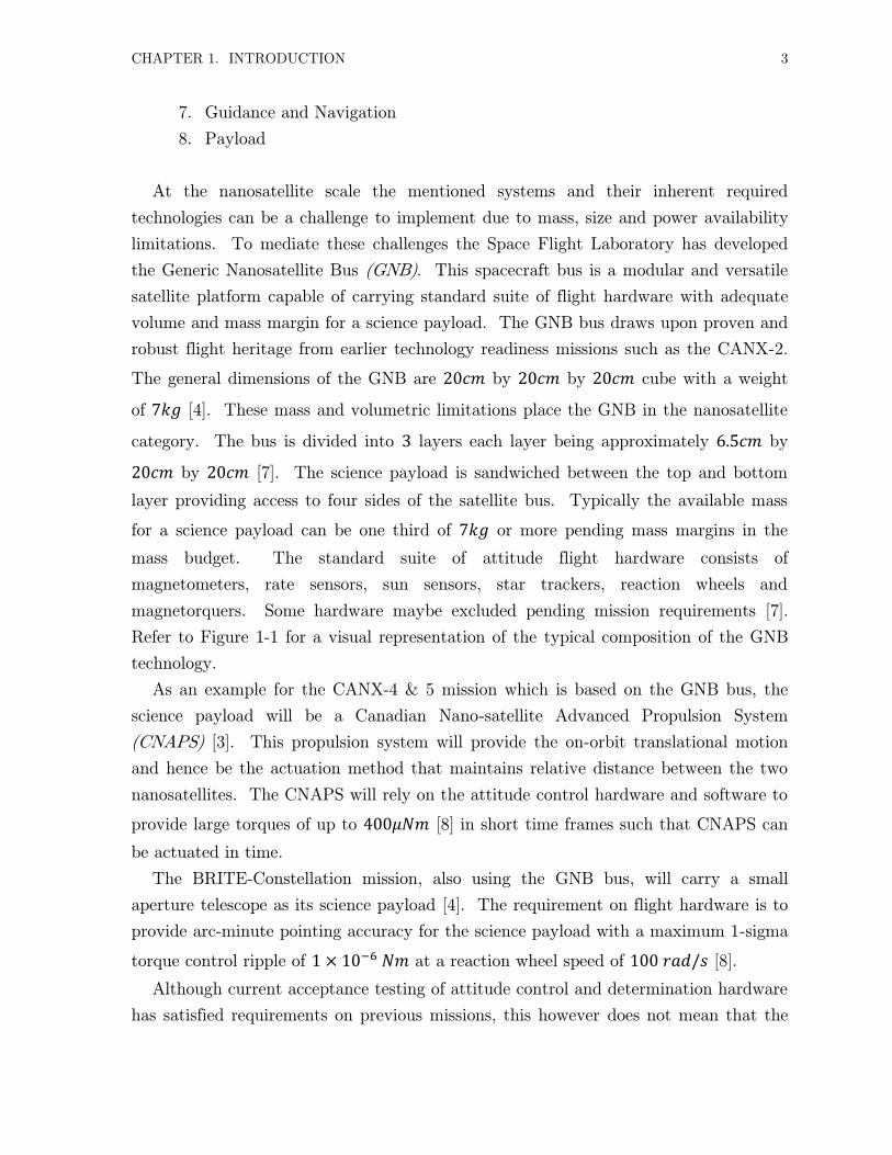
2.6.1. Hysteresis Rod
The hysteresis rod is a piece of ferromagnetic material with specific properties that has
been designed to a particular geometry. The coupling between the geometry and
choice in material provide for a final magnetic permeability which is the relationship
between the magnetic field strength input (Earth magnetic field) and magnetic flux
density (rod magnetic flux density output). The principal of operation is that as the
magnetic field strength input varies due to the spacecraft rotation and orbital position
the rod as a function of magnetic permeability absorbs this field and generates a
magnetic flux density. This process absorbs the energy from the spacecraft angular
momentum and reduces it over time. A sample hysteresis rod designed by the Space
Flight Laboratory (SFL) can be seen in Figure 2-6. More detailed analysis and
acceptance testing of a hysteresis rod is provided in Chapter 4.
Figure 2-6: Space Flight Laboratory (SFL) Hysteresis Rod
2.6.2. Permanent Magnets
The permanent magnet is typically part of a passive attitude control scheme described
at the beginning of this section. It provides a permanent dipole on board the
spacecraft. The limitation is that it can only stabilize a spacecraft about two axes. It
can also add undesired parasitic hysteresis in any ferromagnetic materials that are in
proximity to the dipole on board the spacecraft. This is an effect that is closely
monitored and is minimized in the design process. Part of the work in the hysteresis
rod design is to minimize the effect of the permanent magnet on the hysteresis rods.
A sample permanent magnet can be seen in Figure 2-7. These can be purchased in
many shapes and sizes and have been used quite extensively on nanosatellites.

CHAPTER 2. ATTITUDE CONTROL SYSTEM 23
Figure 2-7: Permanent Magnet
2.7 Acceptance Testing
This chapter has provided the basic foundation on the type of attitude control
hardware that is available for nanosatellite scale of spacecraft and the inherent
limitations. It is important to understand that the acceptance testing process in the
next two chapters provides the link between the requirements and what works in
application (hardware and software). This link corresponds to the gap that must be
crossed in order to verify that the attitude control hardware actually does behave as
required and does so within a certain tolerance. Hence the acceptance testing is
crucial in establishing the foundation of what can be accomplished and what the limits
are in attitude control hardware.

24
Chapter 3
Reaction Wheel Actuator
The reaction wheel actuator at the nanosatellite scale employs a unique design that
balances power consumption, volume, mass and torque output. The two models of
actuators for which the analysis and acceptance testing is shown in this Chapter are
the RW0.03 and RW0.06 reaction wheels. These reaction wheels were developed
jointly between Space Flight Laboratory (SFL) and Sinclair Interplanetary. The
hardware design of these reaction wheels has had previous flight heritage on SFL
missions such as CanX-2 and AISSat-1 [4]. Since their inception the requirements
imposed on these actuators have become more demanding and as such the purpose of
this chapter is to ensure that the most stringent of requirements are met by these
actuators. Hence, the characterization of a reaction wheel, experimental validation of
performance and acceptance testing is presented.
3.1 Principal of Operation
The close examination of a reaction wheel actuator reveals that it is in fact an electric
motor with an oversized rotor. The motor component is essentially a device that
translates the electromotive force (EMF) to a magnetomotive force (MMF) which
acting on permanent magnets embedded in the rotor produce a rotation. This rotation
can be controlled to maintain a state (angular speed) or produce a change in state
(angular acceleration). In a spacecraft, given a particular mass moment of inertia of a
rotor the device will produce a torque about the mass centre when commanded to
produce angular acceleration. This becomes the main linkage between motor design
and attitude control dynamics discussed in Chapter 2.
The motor design can be based on a direct current (DC) or alternating current
(AC) design. The choice is typically DC since the availability of AC power on board a

CHAPTER 3. REACTION WHEEL ACTUATOR 25
spacecraft is non-existent and would require conversion which has inherent losses.
This intrinsic choice is important since a DC design has an extra benefit in that it can
be designed in such a way that the current consumed is proportional to the torque
output of the device [21]. This is extremely beneficial, since given a conversion factor
and through simple current measurements the actuator torque output can be
estimated. Also simplified is the control since the system tends to have a linear
response. The boundaries of this linear response and the inherent non-linearities that
are introduced as a consequence of control and motor design are the focus of this
chapter.
3.2 Reaction Wheel Specifications
The reaction wheels that were analyzed can be viewed on Figure 3-1, where the
relative size of the wheels can be seen. The RW0.03 can be seen on the left and
RW0.06 can be seen on the right of the figure. These reaction wheels differ in their
dimensions, mass and power consumption as shown by Table 3-1, which provides the
specification for these reaction wheels. The similarities are in the DC motor design
and controller behaviour which will be shown in later sections.
Figure 3-1: SFL-Sinclair Interplanetary Reaction Wheels
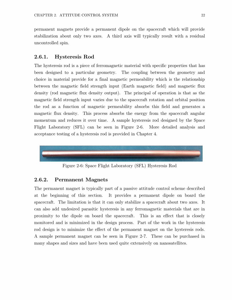
As shown by the specification contained in Table 3-1, these reaction wheels are rated
based on momentum storage and nominal torque output. For the purposes of this
chapter the focus will be on the supply voltage and power consumption which as it
will be shown inherently influence the control torque output. This will become clear in
the next section.
CHAPTER 3. REACTION WHEEL ACTUATOR 26
Table 3-1: SFL-Sinclair Interplanetary Reaction Wheel Specifications
Parameters RW-0.03 RW0.06
Nominal Momentum
Nominal Torque
Control Mode Speed or Torque
Command/Telemetry NSP over UART NSP over UART, RS-485
Mechanical ( ), ( ),
Supply Voltage
Supply Power
Environment Operating temperature
Reliability Diamond coated hybrid ball bearings Redundant motor windings, radiation lot screened parts
3.3 Reaction Wheel Characterization
Prior to actual testing of the RW0.03 and RW0.06 reaction wheels an analytical
approach was taken to predict the performance envelope that could be attained from
each type of wheel. This was done in an effort to better understand what the
performance limits could be and if any undesirable behaviour could exist within the
operating ranges. This type of analysis, as will be shown, also provided the
relationship between power consumption, torque output and speed as a function of
operating at a particular voltage and current.
3.3.1. Performance Assumptions
The performance assumptions that were used in the initial analysis were as shown in
Table 3-1 and the Interface Control Document (ICD) for RW0.03 and RW0.06 which
is readily available and kept current on the Sinclair Interplanetary website. The
purpose of obtaining the specifications and limits was as to estimate the DC motor
performance envelope. It should be understood that this design of a reaction wheel is
essentially a DC motor with an oversized rotor, which focuses the analysis on the DC
motor which is based on electrical and mechanical design.

CHAPTER 3. REACTION WHEEL ACTUATOR 27
The list of the assumptions was as follows for both reaction wheels:
Maximum speed, software limited for both
Maximum torque output
DC Motor Kt and Ke estimate
Winding resistance estimate
Hardware DC current limits
Voltage limits
Rundown data
These were the main performance parameter assumptions into an analytical model
which was then used to generate a performance contour plot as will be shown in later
sections.
3.3.2. DC Motor Characterization
The reaction wheels were based on a Brushless DC Motor (BLDC) design which posed
certain challenges when characterizing these motors. Through detailed analysis of the
BLDC design some limitations were discovered and resultant simplifications had to be
taken in order to provide an accurate characterization. The type of a BLDC design
used was a phase AC motor winding setup coupled with a DC motor control. This
type of a setup can be modelled as a typical DC motor with current telemetry for each
winding. The complication was that only a single current sensor was used to control
the output to the windings which discounted any possibility of current telemetry per
phase. This in turn limited the model of the BLDC motor from a phase to a single
phase model which is the only model that could be experimentally verified and as will
be shown has limitations in the validity of the motor specific constants.
The single phase DC motor model was chosen with the assumption that all three
phases behaved as one and as a result the current and voltage to all phases was the
same due to the single current sensor design. This assumption allowed the use of
equation (3.1) as a DC motor model [22]. This equation allows the representation of
the basic relationship between the voltage, torque, motor constants and motor speed.
The relationships between the described parameters are then used to generate an
analytical power contour plot which predicts the performance envelope of the DC
motor.

CHAPTER 3. REACTION WHEEL ACTUATOR 28
It should be noted that given the availability of current telemetry per phase higher-
order models could have been used providing a more detailed and more accurate
characterization. The motor constants for a single phase model will not be directly
representative of the actual phase motor model constants. Again the single phase
motor model is as follows:
(3.1)
where Voltage applied to the motor windings
Variation of inductance due to moving coil
Winding resistance
Current consumed by motor
Motor speed constant
Motor angular speed.
Assuming a uniform magnetic field within the motor, the relationship between the
current and torque becomes proportional as per equation (3.2):
(3.2)
where Internal motor torque
Motor torque constant
Current consumed by motor.
The relationship between torque and angular speed becomes as shown by equation
(3.3), where the torque is comprised of an angular acceleration term and a term due to
friction. This can be described as follows:
(3.3)
where Mass moment of inertia of motor and load
Angular acceleration of rotor
Opposing torque in motor.

CHAPTER 3. REACTION WHEEL ACTUATOR 29
The opposing torque in motor can be described as shown in equation (3.4):
(3.4)
where Viscous friction torque which is angular speed dependent
Constant friction of the motor
Constant friction of any external load connected to the motor.
Under the assumption of steady state condition with current constant, the equations
(3.1) and (3.2) can be combined to form equation (3.5).
(3.5)
Given the steady state conditions of equation (3.5), when applied torque approaches
zero then the no load velocity becomes as shown in equation (3.6). Consequently the
zero speed stall torque is shown in equation (3.7). These two equations become the
intercept points on a torque-speed curve which shows the relationship between the
speed of the motor and torque. This relationship also shows that the ultimate limit on
speed and torque of the motor is the available voltage:
(3.6)
and
(3.7)
where Internal motor stall torque
Motor angular speed.
The limiting applied voltage in equation (3.6) and (3.7) provides a relationship
between angular speed and torque which is described by equations (3.8) and (3.9).
The speed regulation constant is the slope at the maximum speed that can be attained
given a requested torque. The slope of this line is bounded on one end by the
maximum theoretical speed provided by equation (3.6):

CHAPTER 3. REACTION WHEEL ACTUATOR 30
(3.8)
(3.9)
where Speed regulation constant.
The single phase DC motor equations described thus far pertain to the dynamics of
the motor and provide a variety of relationships which in conjunction with the next
section will be used to provide the analytical power contour plot for the reaction wheel
motor. This is important since this will provide a map of the theoretical performance
that can be obtained from a reaction wheel, which in later work will be validated given
experimental results.
3.3.3. Power Dissipation of DC Motors
The Brushless DC Motor (BLDC) used in the reaction wheel can be considered to be
an energy converter. It converts electrical power to mechanical during any
acceleration or steady state conditions and back to electrical during any deceleration
conditions [22]. Hence, the behaviour of power consumption and dissipation is coupled
with torque and speed and needs to be described in conjunction to the relationships
presented in the previous section. This has obvious implications to a spacecraft power
system where it is important to know how much power the reaction wheel might
demand under required torques and again how much power it might regenerate.
The power conversion and inherent losses in a BLDC motor can be visualized by
Figure 3-2, which shows a flow chart of how the power losses are coupled, where
during the power conversion the motor will have load and speed sensitive losses.
In order to define power consumption we begin with the input power to the motor
which can be described by equation (3.10). One main assumption is that the motor
behaves as a linear resistive load:
(3.10)
where Power input to the motor.

CHAPTER 3. REACTION WHEEL ACTUATOR 31
Assuming steady state conditions and substituting equation (3.1) into (3.10), we get
input power as a function of motor losses shown in equation (3.11):
(3.11)
Combining (3.2), (3.3), (3.4) and (3.11) with the exclusion of which corresponds to
losses due to mechanical coupling between motor and an external load, we get
equation (3.12). The result describes in a general sense the instantaneous power
dissipation given a torque load and motor losses of a BLDC motor. The motor
frictional losses can be quantified through further friction modelling. Hence the
instantaneous dissipative power can be described by:
(3.12)
Input
Power
Power
Conversion
Output
Power
Motor
Losses
𝐼𝑎 𝑅
Winding Eddy
Currents Hysteresis
Windage
Friction
Short
Circuit
Currents
Speed Sensitive Load (Torque)
Sensitive
Figure 3-2: Power Losses in Brushless DC Motor (BLDC) Design

CHAPTER 3. REACTION WHEEL ACTUATOR 32
3.3.4. Modeling Friction
The losses due to friction in a BLDC motor as shown in equation (3.4) can be
rewritten without and as a function of constant and speed sensitive losses as shown
in (3.13). As mentioned earlier the component is being omitted since the reaction
wheel is not coupled mechanically to any external loads. This result is a polynomial
which can be extracted through a curve fit of the motor free-spinning spin down.
Hence the opposing torque can be described by:
(3.13)
The modelling of friction was accomplished using previously recorded reaction wheel
speed rundown data as a function of time. The reaction wheel started the rundown at
an approximate speed of . Data in the negative and positive rundown
profiles was curve fit using a polynomial function. The terms in the resultant
polynomial are a representation of the opposing torque described by equation (3.13).
An example of the opposing friction is provided in the Section 3.4 of this chapter.
3.3.5. Analytical Dissipative Power Contour Plot
The initial dissipative power contour plot is based on the single phase DC motor
model, power dissipative model and friction approximation from past reaction wheel
data as previously described. This plot provides the power consumption of the
reaction wheel given a torque and speed state. The plot is generated using equations
(3.5) and (3.12), which describe the relationships between power, current, voltage,
speed and torque. The initial plots can be seen in Figure 3-3 for the RW0.03 reaction
wheel and Figure 3-4 for the RW0.06 reaction wheel.
These plots show the speed of the reaction wheel on the x-axis, the torque on the y-
axis and the coloured contours correspond to consumed or regenerated power. The
positive contours represent power consumed and the negative contours represent power
regenerated. Also the lines that appear in parallel show the limits as a function of
voltage and current, where the current limits the maximum torque that can be
obtained and the voltage limits the maximum speed. Plotted is the rundown data
that had been used for modelling friction, which also shows the power, torque and
speed envelopes within which the wheel has previously operated. The area on the plot
where the rundown data is parallel to the voltage lines corresponds to the speed

CHAPTER 3. REACTION WHEEL ACTUATOR 33
regulation constant as described by equation (3.9). This was the initial attempt to
estimate BLDC motor performance.
Figure 3-3: RW0.03 Analytical Power Contour Estimate
Figure 3-4: RW0.06 Analytical Power Contour Estimate
RW0.03 Dissipative Power
RW0.06 Dissipative Power
Speed (rad/s)
Speed (rad/s)
Gen
era
ted T
orq
ue (
Nm
) G
en
era
ted T
orq
ue (
Nm
) Plotted
rundown
data
Plotted
rundown
data
CHAPTER 3. REACTION WHEEL ACTUATOR 34
Detailed analysis of these plots has shown that the following limitations exist with the
current reaction wheels:
RW0.03 Estimates
o Peak power consumption of 1.5W
o Peak regeneration of 1W
o Maximum speed of 970 rad/s at 6VDC
RW0.06 Estimates
o Peak power consumption of 7W
o Peak regeneration could be 4W
o Maximum speed of +1600 rad/s at 28VDC
Both reaction wheels showed large torque overshoot during zero
crossings
The above information was instrumental in providing direction for further
experimental testing of reaction wheels. The power peak consumption was confirmed
against reaction wheel specifications shown earlier in Table 3-1. It can be seen that
these were reasonable. The estimates of the regeneration zones of the DC motor were
apparently being avoided through the use of a power controller in the reaction wheel
software. The concern was still present that the reaction wheel motor could regenerate
and as such a shunt resistor was chosen to protect the DC motor. It is important to
protect against regeneration since a DC motor is the only path of resistance and the
regeneration can short out through the motor causing damage. Further discussion on
shunt resistor sizing and reaction wheel safety is provided in Section 3.7. Finally the
torque performance, speed limits and overshoot behaviour was chosen to be verified.
The analytical power contour estimate provided the following key aspects of the
RW0.03 and RW0.06 reaction wheel DC motors that needed to be verified prior to the
commencement of acceptance testing:
Peak power consumption
Peak regeneration
Maximum speeds at operating voltage
Overshoot behaviour at zero crossings
Torque response

CHAPTER 3. REACTION WHEEL ACTUATOR 35
3.4 Experimental Verification of Model
The experimental verification of the reaction wheel DC motor model was completed to
calibrate and verify the analytical results shown in the previous section. This is
important since the characterization map can be used to choose performance envelopes
in acceptance testing such that requirements are met. The testing was performed
using RW0.03 and RW0.06 reaction wheels.
3.4.1. Test Methodology
The test methodology consisted of operating each type of reaction wheel through
speed, torque and digital to analog converter (DAC) profiles. These profiles were
termed speed box, torque box and DAC box. In addition, rundown data was to be
captured, providing an update to the opposing friction estimate. In an effort to ensure
maximum data resolution and correct time stamping the data acquisition process was
reviewed, and best practice was established.
The speed box profile commanded the reaction wheel from its most negative speed
to its most positive speed and back again. The telemetry that was polled was speed
and time. This provided for a confirmation of the maximum speed envelope at
incremental voltages that were to be required for acceptance testing. The overall
response of the speed controller was measured through this profile.
The torque box profile commanded the reaction wheel through steps of torque.
Each torque was applied at the maximum opposing speed providing a torque response
map in all four motor quadrants. It was determined early in testing that the torque
telemetry from the reaction wheel was too noisy and would not provide meaningful
results. The data polled ended up being speed and time and in post processing the
incremental torque was determined. This profile captured the overall response of the
torque controller.
The digital to analog converter is an open loop command to set a duty cycle for the
motor output to the windings. This profile sets the duty cycle output in increments
and polls the current with time as telemetry. This was an attempt to measure the
maximum possible regeneration that the motor could encounter.
All testing for both the RW0.03 and RW0.06 was completed using a shunt resistor
as defined in Section 3.7. In addition to the reaction wheel telemetry, external current
was recorded throughout all testing to measure and confirm externally the dissipative
power behaviour of the reaction wheel.

CHAPTER 3. REACTION WHEEL ACTUATOR 36
3.4.2. System Limitations
The testing was limited by a number of factors which were inherent to the design of
the reaction wheel. Some observed notable limits were:
Only parameter can be polled at a time
Resolution of the reaction wheel data is limited by the data communication
interface
External current measurements were limited to
Application interface to the reaction wheel was on a Microsoft Windows
platform which added complexity as shown in Section 3.4.4
3.4.3. Test Setup
The primary concern during testing was the safety of the reaction wheels actuator
since some were intended for flight. For this reason the reaction wheels were mounted
in a protective enclosure with a dedicated harness routed to each reaction wheel. This
allowed for the device to be fully isolated and safe for bench top testing. Below Figure
3-5 shows four RW0.06 reaction wheels in an enclosure.
Figure 3-5: RW0.06 Reaction Wheel Enclosure

CHAPTER 3. REACTION WHEEL ACTUATOR 37
The interface between the reaction wheel and the control software is shown by Figure
3-6. The test setup consisted of the following items:
Reaction wheel enclosure with reaction wheels
Isolated variable DC power supply rated for the operating voltage of the
reaction wheels
Shunt resistor rated for estimated regeneration of reaction wheels with a
safety margin
Communication converter for signal levels
PC with Microsoft Windows XP and a free communication port capable
of , and , baud rates
Wheelterm interface application
Figure 3-6: Reaction Wheel Test Setup
3.4.4. Acquisition of Data
Prior to any testing it was critical to identify the maximum reliable data polling rates
that could be obtained for the RW0.03 and RW0.06 reaction wheels. Two
requirements had to be met: first, correct time stamping had to be implemented, and
second, there was not to be any packet loss while maximizing the polling rate. Using
an oscilloscope a test was performed measuring the lag of the wheel response. This
was in an effort as to determine the limiting factor in communications. It was
measured that the reaction wheel interface response to a telemetry packet request had
Reaction Wheel
RW0.03 or RW0.06
Windows OS
Wheelterm
Interface
COM PORT
(RS232)
TO
TTL Converter
(RS485/UART)
DC Power
Supply
Shunt
Resistor
Reaction Wheel Test Setup
Com
munic
ati
on
Pow
er

CHAPTER 3. REACTION WHEEL ACTUATOR 38
a maximum of of delay, while the lag of Wheelterm (interface application)
sending the next command was . The wheel packet response lag to a packet
request can be seen on Figure 3-7, where the wheel response is only behind the
wheel command. Based on the limiting latency it was determined that the
maximum polling rate of the interface to the reaction wheel could not exceed .
The next step was to determine at what polling frequencies of equal to or less than the
maximum can the data with no packet loss and correct time stamp be acquired.
Testing was performed on RW0.03 and 4 RW0.06 reaction wheels. The results
showed that consistent time stamps and no packet loss could only be acquired during
and polling rates. Figure 3-8 shows the results for RW0.03 data time
stamp and packet loss, where the correct torque jitter of less that
identifies valid polling results. It should be noted that up to this point the polling
rates that had be used were less than with some packet loss. Some adjustments
had to be made during the RW0.06 testing which included a longer than typical
communication cable as a consequence of the enclosure. The longer cable caused some
packet loss initially but was remedied by adding a termination resistor which is
required by the RS485 standard.
Wheel Response
Wheel Command
Figure 3-7: RW0.03 Communication Interface

CHAPTER 3. REACTION WHEEL ACTUATOR 39
Through all the testing there was no difference in the results obtained between the
RW0.06 and RW0.03, which also supported that the limiting factor in the current test
scheme is the Windows environment. It is speculated that the Windows kernel is
limited to a scan cycle of the communication port which cannot be changed.
Future considerations were to utilize an embedded test platform or a Linux based
system in an effort to reduce latency. This work established best practice for
communication interfacing during testing of reaction wheels.
Figure 3-8: RW0.03 Data Polling Frequency Comparison
3.4.5. Verification of Friction Estimate
Given the verified data acquisition interface, confirmation of reaction wheel friction
was obtained. This estimate was done to confirm the friction estimate that was
derived from past reaction wheel rundown data as discussed in Section 3.3.4. The
secondary benefit of this estimate confirmation was that the new set of data provided
the friction estimate with a higher resolution. The data for both RW0.03 and RW0.06
was fitted using a second order polynomial to ensure that the first two terms of
friction are captured according to (3.13). The results for the RW0.03 reaction wheel
are shown in Figure 3-9, and for RW0.06 reaction wheel in Figure 3-10. These results
were implemented in the power contour map for the reaction wheels as is shown in the
next section.
0.0
0.5
1.0
1.5
2.0
2.5
3.0
3.5
4.0
0 1 2 3 4 5 6 7 8 9 10 11 12 13 14 15 16 17 18 19 20 21
Torq
ue
Jit
ter
(𝜇N
m)
Reaction Wheels 1 to 21
Reaction Wheel Torque Jitter as a Function of Polling Frequency
62Hz
32Hz
21Hz

CHAPTER 3. REACTION WHEEL ACTUATOR 40
Figure 3-9: RW0.03 Opposing Torque Estimate
Figure 3-10: RW0.06 Opposing Torque Estimate
0.0E+00
5.0E-05
1.0E-04
1.5E-04
2.0E-04
2.5E-04
3.0E-04
3.5E-04
4.0E-04
150 250 350 450 550 650 750
Op
po
sin
g T
orq
ue
(µ
Nm
)
Reaction Wheel Speed (rad/s)
RW0.03 Opposing Torque Estimate
0
0.01
0.02
0.03
0.04
0.05
0.06
0 200 400 600 800 1000 1200
Op
po
sin
g To
rqu
e (𝜇
Nm
)
Reaction Wheel Speed (rad/s)
RW0.06 Opposing Torque Estimate

CHAPTER 3. REACTION WHEEL ACTUATOR 41
3.4.6. DAC Box
The Digital to Analog Converter (DAC) Box is a test where the wheel controller
actuates its drive stages to the motor windings in open loop. This is essentially the
final output where the digital to analog conversion is performed between the
microcontroller and an analog output signal to the drive stages. The test actuates a
set of open loop DAC commands which drive the reaction wheel motor at a maximum
and only hardware limited output. The result is a torque response versus the speed at
different voltage levels against a power contour plot.
The RW0.03 reaction wheel was tested showing the results in Figure 3-11. The
results showed a very clear behaviour in the second and fourth quadrant where the
motor did not enter the regenerative zones. This had also been confirmed by external
current measurements showing no regeneration. The plot also showed the maximum
power consumed across the speed envelope given a constant voltage and power
tracking in first and third quadrant. This test confirmed the power contour plot and
the underlying estimated motor parameters. It also confirmed that during DAC
commands the motor will not enter into regeneration. Although DAC mode will not
be used on board the spacecraft, it is an important step in verifying the
characterization through open loop control and before closed loop control is tested.
Figure 3-11: RW0.03 DAC Box Results
RW0.03 Dissipative Power – DAC Box
Gen
era
ted T
orq
ue (
Nm
)
Speed (rad/s)
4VDC
5VDC
6VDC

CHAPTER 3. REACTION WHEEL ACTUATOR 42
The RW0.06 reaction wheel DAC test results can be viewed on Figure 3-12. These
results are only shown for the regenerative quadrant which is the second or fourth
quadrant. The results do not differ between the described quadrants hence only one
quadrant is shown. Given the DAC commands the motor does enter regenerations of
almost and at a DAC command of . This shows that the previously described
assumption that no regeneration will occur has been invalidated and the motor will
show regeneration. The power tracking as with the RW0.03 was also confirmed with
external current telemetry validating the characterization. The areas of interest from
this test were the regeneration and increased torque jitter during regeneration.
The regeneration is of concern since it may exist during closed-loop control in the
Speed and Torque Box tests. This behaviour would impact the spacecraft power
system and/or reaction wheel if an appropriate shunt load is not integrated. The
excessive torque jitter can provide diminished performance pending the operating
speed of the reaction wheel during spacecraft operations. Further testing provided
more detail on both behaviours in closed loop form which is the operating mode on
board spacecraft.
Figure 3-12: RW0.06 DAC Box Results
RW0.06 Dissipative Power – DAC Box
Speed (rad/s)
Gen
era
ted T
orq
ue (
Nm
)

CHAPTER 3. REACTION WHEEL ACTUATOR 43
3.4.7. Speed Box
The Speed Box test provided the first closed loop response in comparison to the DAC
Box test. This test uses a dual loop control with two PID controllers. The reaction
wheel operates a speed control loop at an approximate rate of and a second
power tracking control loop in the range of . These loops are controlled
through user defined set points. The speed control loop set point commands the
reaction wheel speed and the power control loop set point commands the maximum
power the reaction wheel can consume in the first or third quadrant. This test shows
the coupled behaviour between both controllers. The control mode can be used on
board the spacecraft and is the next logical step from the DAC open loop control.
The RW0.03 reaction wheel results can be seen in Figure 3-13. Where again as
with the DAC Box results there was no regeneration shown. Although there was a
progressively worse torque jitter behaviour in the regenerative quadrants and a poor
zero crossing behaviour. The power tracker can be seen tracking in both the
first and third quadrants which validates both the estimated motor parameters and
the friction estimate. The validation comes from the measured response which is the
plotted data matching the predicted power contour lines, voltage, torque and speed.
Figure 3-13: RW0.03 Speed Box Results
RW0.03 Dissipative Power – Speed Box
Gen
era
ted T
orq
ue (
Nm
)
Speed (rad/s)

CHAPTER 3. REACTION WHEEL ACTUATOR 44
The RW0.06 as with the RW0.03 uses the same control loops. In fact both reaction
wheels have identical microprocessors and only differ in the final MOSFET drive
stages. Figure 3-14 shows results for RW0.06, which showed regeneration of almost
, increased torque jitter in regenerative zones and large torque overshoot during
zero crossings. The power controller can be seen tracking approximately in the
first and third quadrant which is as expected. The characterization was confirmed by
matching power contour lines, voltage torque and speed response.
Figure 3-14: RW0.06 Speed Box Results
3.4.8. Torque Box
The Torque Box provides a final result of the torque closed loop controller coupled
with the power tracking controller given a variation in torque commands. This control
mode is the same control mode that is used on-board the spacecraft. The controller
essentially tracks an angular acceleration up to the maximum speed. The regenerative
zones and torque behaviour across the reaction wheel speed range is of importance in
this final confirmation of characterization.
The RW0.03 results can be seen in Figure 3-15. The results show clear regeneration
during torque commands as opposed to no regeneration shown by the previous two
tests. This regeneration was also confirmed with external current telemetry showing a
RW0.06 Dissipative Power – Speed Box
Speed (rad/s)
Gen
era
ted T
orq
ue (
Nm
)

CHAPTER 3. REACTION WHEEL ACTUATOR 45
peak of . There is also an increase in torque jitter more than seen with the
Speed Box during speed control in the regeneration zones. The zero crossing torque
jitter has also increased. Overall the characterization had been confirmed and a
regenerative behaviour of the RW0.03 had been discovered.
Figure 3-15: RW0.03 Torque Box Results
The RW0.06 reaction wheel Torque Box results can be seen in Figure 3-16. Where the
same behaviour is seen with the regeneration and torque jitter as seen in two previous
tests. Regeneration of a maximum of was detected at the highest torques that
would be expected on orbit. The characterization had been confirmed against the
measured response of the reaction wheel.
The testing of both of the reaction wheel actuators had confirmed the following
behavioural areas that need to be considered for acceptance testing:
Regeneration impact on reaction wheel and/or power system
Zero crossing torque response
Torque jitter in regenerative zones
Best operating zones for minimal torque jitter
The identified concerns are further investigated in later sections.
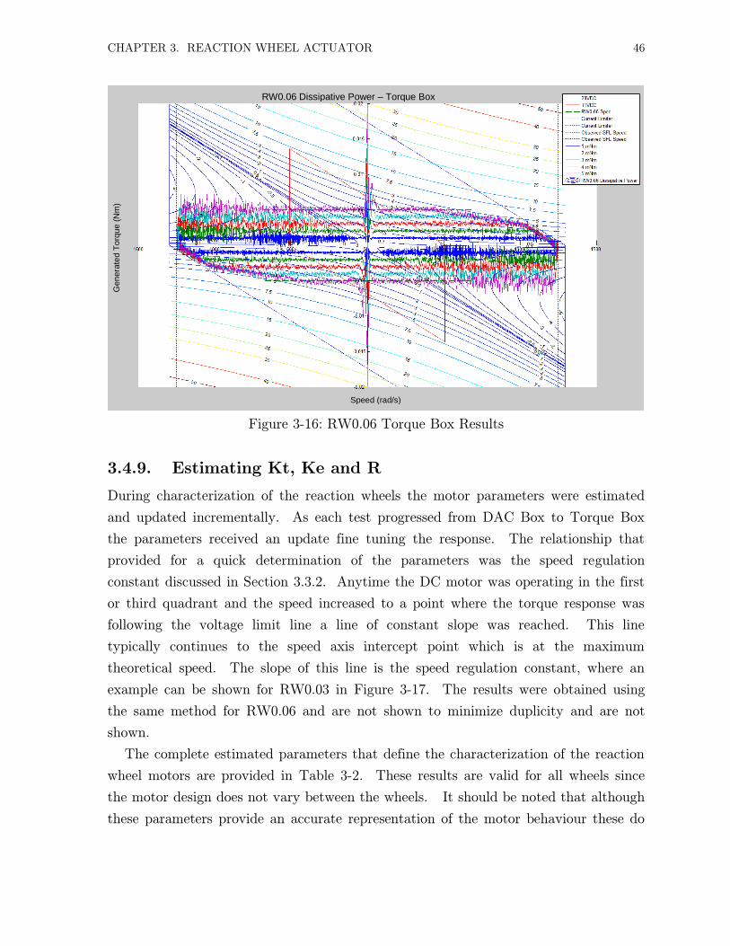
CHAPTER 3. REACTION WHEEL ACTUATOR 46
Figure 3-16: RW0.06 Torque Box Results
3.4.9. Estimating Kt, Ke and R
During characterization of the reaction wheels the motor parameters were estimated
and updated incrementally. As each test progressed from DAC Box to Torque Box
the parameters received an update fine tuning the response. The relationship that
provided for a quick determination of the parameters was the speed regulation
constant discussed in Section 3.3.2. Anytime the DC motor was operating in the first
or third quadrant and the speed increased to a point where the torque response was
following the voltage limit line a line of constant slope was reached. This line
typically continues to the speed axis intercept point which is at the maximum
theoretical speed. The slope of this line is the speed regulation constant, where an
example can be shown for RW0.03 in Figure 3-17. The results were obtained using
the same method for RW0.06 and are not shown to minimize duplicity and are not
shown.
The complete estimated parameters that define the characterization of the reaction
wheel motors are provided in Table 3-2. These results are valid for all wheels since
the motor design does not vary between the wheels. It should be noted that although
these parameters provide an accurate representation of the motor behaviour these do
RW0.06 Dissipative Power – Torque Box
Speed (rad/s)
Gen
era
ted T
orq
ue (
Nm
)

CHAPTER 3. REACTION WHEEL ACTUATOR 47
not represent the motor design parameters since the model used to describe the motor
is single phase and not a phase model as described in Section 3.3.2.
Figure 3-17: RW0.03 Regulation Speed Constant
Table 3-2: Reaction Wheel DC Motor Parameter Estimates
Parameters RW0.03 RW0.06
Voltage (VDC)
Duty Cycle (%)
Kt (Nm/A)
Ke (Vs/rad)
Max. Speed (rad/s)
Winding Resistance (Ω)
Speed Regulation Constant
400
450
500
550
600
650
700
0 200 400 600 800 1,000 1,200 1,400
Re
acti
on
Wh
ee
l Sp
ee
d (
rad
/s)
Torque Applied (𝜇Nm)
RW0.03 Speed Regulation Constant

CHAPTER 3. REACTION WHEEL ACTUATOR 48
3.5 Torque Controller Improvement
The characterization of the reaction wheel motor showed that regeneration is present
during torque operation of the both the RW0.03 and RW0.06 reaction wheels. The
data also showed an increase in torque jitter. This section provides a more in-depth
look at the torque jitter during regeneration and identifies actions that had been taken
to remedy jitter increase.
3.5.1. Torque and Speed Controller Comparison
The torque and speed controller responses were compared to shed light on the
increased torque jitter behaviour during closed loop torque control mode. The results
for the RW0.06 can be seen as an example in Figure 3-18. Where on the left is the
speed controller showing regeneration and on the right is the torque controller in
regeneration showing increased torque jitter and poor zero crossings. Similar
behaviour was found in the RW0.03 reaction wheel with the exception of no
regeneration in DAC and speed control mode.
Figure 3-18: RW0.06 Torque and Speed Controller Comparison
Speed Control Torque Control
Zero crossing
Regeneration
Torque Jitter
RW0.06 Speed and Torque Controller Regeneration
Time (s)
Pow
er
(W)

CHAPTER 3. REACTION WHEEL ACTUATOR 49
A closer look at the torque jitter during torque control regeneration for RW0.03 can be
seen in Figure 3-19, where a periodic pattern can be seen which suggests a control
scheme used in the software of the reaction wheel. The reaction wheel does enter
regeneration and seems to attempt to recover from regeneration.
Figure 3-19: RW0.03 Regeneration During Torque Command
The RW0.06 reaction wheel result can be seen in Figure 3-20, showing similar
behaviour to the RW0.03. Through further analysis of the reaction wheel software
and hardware it was determined that the software invokes a regeneration control.
This control behaviour is the resultant controller regeneration shown for RW0.03 and
RW0.06 where the controller attempts to jump across the regeneration zone but fails
during part of the cycle. This behaviour had been confirmed during testing with a
variation of torques with external current measurements at .
The analysis also revealed that the zero crossings have poor performance due to the
hall effect sensor speed estimation scheme used in the reaction wheels. The speed
estimation essentially determines the time from one hall effect sensor to the next. As
the motor approaches a zero crossing the time between sensor counts increases and the
Curr
ent
(A)
Time (ms)
RW0.03 Torque Controller Regeneration

CHAPTER 3. REACTION WHEEL ACTUATOR 50
state of the reaction wheel becomes undetermined. The PID responsible for
controlling the torque begins to overshoot as the time between sensor counts increases.
The torque controller undershoots once the zero point has been crossed and the time
between the sensor counts decreases. Hence, the analysis thus far suggests that the
zero crossings and increased torque jitter could be improved through a reaction wheel
control software update. The degree of improvement and timeline of when it will be
done had not been determined at the time of writing this thesis.
Figure 3-20: RW0.06 Regeneration During Torque Command
3.5.2. Software Modification for Improved Torque Performance
Given the torque jitter during regeneration and zero crossing response a software
update was in the works at the time of writing this thesis. This software update
would provide an improved reaction wheel zero crossing response through the use of a
new speed estimation scheme. The regeneration control would also be either removed
or improved on. The reaction wheels used for characterization and acceptance testing
in this thesis did not use this software update.
RW0.06 Torque Controller Regeneration
Pow
er
(W)
Time (s)

CHAPTER 3. REACTION WHEEL ACTUATOR 51
3.6 Regeneration Effect on Spacecraft Power Board
The characterization results predicted and verified the regenerative behaviour of the
RW0.03 and RW0.06 reaction wheels. This result showed that if regeneration is
invoked on-orbit during spacecraft operations the power bus of the spacecraft must
absorb this regeneration safely. When considering the spacecraft power bus, two
requirements were derived. The first requirement was in regards to the shunt size that
would absorb the regeneration. The second was the requirement of the power switch
for the reaction wheel being able to handle the regenerative current in the off state.
Through testing and not part of this thesis, it was verified that the spacecraft
battery will adequately behave as a shunt and absorb the assumed maximum of
for the RW0.06 reaction wheel and for RW0.03 reaction wheel. This analysis
verified the first requirement.
The second requirement was verified against the operation of the power switch for
the reaction wheel. Details of the setup and analysis are further described in the
sections that follow.
3.6.1. Power Board Principle of Operation
The spacecraft power board is responsible for all power generation, supply and storage
on board the spacecraft. This system manages the battery and solar cell power
generation through what is called a Battery Charge and Discharge Regulator using
high efficiency methods for peak power tracking [23]. It also manages power
consumption by devices and is capable of intelligently switching off loads in case of
over current or to simply cycle power on a device. The overall implication is that for
the spacecraft to be successful it must stay power positive and this system does just
that. Hence, the importance of verifying requirements imposed by other systems
becomes crucial for the success of the mission.
3.6.2. Actuator Integration
Both types of reaction wheels tested in this thesis use a single port for combined power
and communications. This port is typically connected directly to the power board
which separates the power feed to the connector from the communication feed. The
power feed is then connected to a dedicated switch on the power board. This switch
can be a simple MOSFET or it could be more complex with added circuitry of over
current protection [23]. The power board has the ability to switch the device on and

CHAPTER 3. REACTION WHEEL ACTUATOR 52
measure its power consumption. It is important to realise that past the on/off switch
for a reaction wheel, all devices connected to the power bus share that power. The
implication is that if a device produces noise all other devices must be able to mitigate
this noise.
3.6.3. Regeneration Test Setup
The test was performed using a sample spacecraft power board in a configuration with
the reaction wheel as would be integrated on board spacecraft. A DC power supply
was used to supply a bus voltage. Current readings were obtained through telemetry
from the reaction wheel and the power board. The test setup consisted of the RW0.03
and RW0.06 reaction wheel, shunt resistors, power board, DC power supply, windows
PC and oscilloscope.
The reaction wheel was placed into a state from which once power cycled would
produce maximum regeneration. This typically meant spinning up the reaction wheel
to a maximum speed and applying a reverse torque at which point the power board
switch was turned off. Throughout the test, the current and voltage telemetry was
being recorded
3.6.4. Regeneration Results
The results can be broken down into three individual events which can be seen on
Figure 3-21. Each event is composed of a voltage and current. The current can be
either flowing to or from the reaction wheel. The state of the wheel is determined as a
function of voltage and current. The reaction wheel is commanded by a DAC
command of which was previously shown in Section 3.4.6 to produce maximum
regeneration. Only reaction wheel RW0.06 results are shown since this reaction wheel
produced the most regeneration and represented the worst case scenario.
The first event shows the command sent to the reaction wheel and then the power
switch turned off. The rise in voltage (yellow line) above the initial voltage and the
negative spike in current (pink line) show that the regenerated current was flowing
across the body diode of the switch (MOSFET) to the spacecraft bus. This continued
until the reaction wheel generated voltage dropped back down to the magnitude of the
initial bus voltage.
The second event is the voltage continuing to drop below bus voltage and until the
microprocessor loses power at . The current shows regeneration that is
decreasing progressively. The current is being sunk by a local zener diode that is part

CHAPTER 3. REACTION WHEEL ACTUATOR 53
of the local switch circuitry. This generated a requirement for the zener diode to
ensure that it can handle the amount of power in this configuration. Testing of zener
diode and verification against manufacturers specifications showed that the power
levels are well within tolerance for nominal operation.
The third and last event shows that the voltage has diminished to almost zero and
that the opposing torque is greater than any regenerated current. In this event the
reaction wheel microprocessor is unpowered and the reaction wheel is coasting down
under its own friction.
Figure 3-21: Reaction Wheel Power Switch Test
3.6.5. Summary of Results
In summary, the analysis of the test results had shown that the power board can
absorb the worst case regeneration of approximately . This was confirmed with the
reaction wheel power switch on and off. No additional shunt resistor was required in
addition to the battery during regeneration. The impact of the regeneration that was
identified in motor characterization has been assessed and retired through testing.
Voltage
Current

CHAPTER 3. REACTION WHEEL ACTUATOR 54
3.7 Safe Operation
The operation of the reaction wheel needs to be safely performed on board the
spacecraft and during testing. In the previous section the safe operation of the
reaction wheel on board spacecraft was confirmed with the testing of the power board.
This section describes a safe method that was used for all ground testing of the
reaction wheels.
3.7.1. DC Motor Regeneration
The regeneration that is generated from a reaction wheel must be externally absorbed
such that the regenerative current does not flow back into the reaction wheel. This is
critical since the reaction wheels drive stages can be easily damaged if enough reverse
current is absorbed. This damage may not be immediate and it could become evident
through diminished performance on one of the drive stages. The overall effect would
be a drastic reduction in torque control performance. Hence, it is best practice to
avoid regeneration through the use of an external shunt. The regeneration that the
shunt must be rated for is:
for RW0.03
for RW0.06
3.7.2. Shunt Resistor Sizing
The shunt resistor is sized for the peak regenerative power of the device. In addition,
a consideration had to be given if more than one reaction wheel would be tested at a
time. Due to power supply limitations and communication interface best practice
described in Section 3.4.4 a single wheel test was deemed adequate. This meant that
each wheel would have its own shunt resistor with its own communication interface
operating at the polling frequency. This configuration would in effect maximize
protection against regeneration and maximize the communication bandwidth.
The selection of shunt resistors for the RW0.03 reaction wheel is shown in Table
3-3, while the selection of shunt resistors for RW0.06 reaction wheels is shown in Table
3-4. The final chosen resistor configuration was:
RW0.03: resistor with a rating for wheel
RW0.06 Resistor with rating for wheel
More specifically, the values of resistance and power rating were obtained by
comparing the amount of regenerative current at different voltages that a resistor

CHAPTER 3. REACTION WHEEL ACTUATOR 55
would have to absorb as shown by the shunt resistor sizing tables. In addition the
configuration of multiple and single wheels on the same bus was compared. For both
the RW0.03 and RW0.06 the critical metric that must have been met was that the
power supply current must be greater than the regeneration current. The final resistor
choice was based on power supply availability and a safety margin which
accounted for the regenerative current as can be seen in the provided results.
DC
M
Power Supply28VDC <-> 11VDC
Resistor (Shunt) 20Ω 50W
RW0.06 Reaction Wheel
Figure 3-22: Reaction Wheel Safe Setup Example
The shunt resistor connection is in parallel to the reaction wheel and DC power
supply. Figure 3-22 shows the configuration for the RW0.06 reaction wheel. The
RW0.03 reaction wheel has the same configuration except for the DC power supply
and shunt resistor rating being as per Table 3-3.
Table 3-3: RW0.03 Shunt Resistor Sizing
RW0.03 Reaction Wheel Shunt Resistor Sizing
Parameters 1 - Reaction
Wheel 6-Reaction
Wheels
Regeneration Power (W) 1 6
Operating Voltage (VDC) 3.4 6 3.4 6
Regeneration Current (A) 0.29 0.17 1.76 1.00
Required Resistance (Ohm) 11.56 36.00 1.93 6.00
Chosen Resistor (Ohm) 10 10 1.5 1.5
Power Supply Current for Resistor (A) 0.34 0.60 2.27 4.00
Power Rating for Resistor (W) 1.16 3.60 7.71 24.00

CHAPTER 3. REACTION WHEEL ACTUATOR 56
Table 3-4: RW0.06 Shunt Resistor Sizing
RW0.06 Reaction Wheel Shunt Resistor Sizing
Parameters 1 - Reaction
Wheel 4-Reaction
Wheels
Regeneration Power (W) 5 20
Operating Voltage (VDC) 11 28 11 28
Regeneration Current (A) 0.45 0.18 1.82 0.71
Required Resistance (Ohm) 24.2 156.8 6.05 39.2
Chosen Resistor (Ohm) 20 20 5 5
Power Supply Current for Resistor (A) 0.55 1.40 2.20 5.60
Power Rating for Resistor (W) 6.05 39.2 24.2 156.8
3.7.3. Verification of Safe Operation
The operation of the reaction wheel with the shunt resistor had been verified with
external current measurements. The current flow was confirmed to always be away
from the reaction wheel, which meant that the path of lowest resistance was the shunt.
This configuration was also monitored for temperature as to make sure that excessive
heating is not generated. This work established a verified method of safely ground
testing of reaction wheels.
3.8 Typical Acceptance Test
All analysis shown up to this point of this chapter has provided for the foundation
necessary to perform acceptance testing. The reaction wheel motor characterization
has established at what speeds the reaction wheel can attain minimum torque jitter.
The communication interface analysis has provided the highest and most reliable data
polling frequency providing for maximum data resolution. The regeneration analysis
has ensured safe testing of reaction wheels. In summary, this section will provide an
overview of the acceptance test plan and sample results for the RW0.03 and RW0.06
reaction wheels.
The acceptance testing was performed for a number of missions under development
at the Space Flight Laboratory. These missions were BRITE-Canada, AISSat-2,
CanX-4/-5 and NEMO-AM. In total RW0.03 and RW0.06 reaction wheels were
tested and verified against requirements. Typically the acceptance test is catered
towards the requirements of a particular mission.

CHAPTER 3. REACTION WHEEL ACTUATOR 57
The acceptance testing is divided into three sections: nominal performance, torque
performance, and operation over temperature. The nominal performance section
verifies that the reaction wheel is in fact operating as it should in terms of the
standard parameters such as speed noise, power consumption and damping coefficient.
This section is composed of the following tests:
Burn-in
Short Form Functional Fest (SFFT)
Speed Noise Test
Power consumption
The torque performance section is comprised of a variety of torques tests. These tests
are established as a function of requirements. The input is the different speeds from
which the reaction wheel will be applying a torque. The output is a number of torque
metrics including torque jitter. The operation over temperature uses tests from
previous two sections at different temperature plateaus. The next section will begin
with a description of the tests in a sequential order with sample results.
3.8.1. Burn-in
The burn-in is a method of breaking-in the reaction wheel. This is performed initially
upon the receipt of the reaction wheel and prior to any actual testing. The burn-in is
comprised of a cycling of speed between the positive and negative speed envelopes over
a period of . The intent is to break-in the bearing and grease of the reaction
wheel. This is intended to reduce the initial friction to a lower and more constant
friction response which is seen in post burn-in.
3.8.2. Short Form Functional Test
The Short Form Functional Test (SFFT) actuates the reaction wheel through a set of
commands and measures the response. This response is then compared against typical
operational ranges. The test ensures that the reaction wheel is performing nominally
as compared to accepted values. The test is comprised of the following sequence of
commands:
Maximum positive and negative speed with no power limiter
Maximum positive and negative speed with power limiter
Speed steps

CHAPTER 3. REACTION WHEEL ACTUATOR 58
Torque steps
The data is collected and parsed using MATLAB. The typical results can be seen in
Figure 3-23 for the RW0.03 and Figure 3-24 for the RW0.06 reaction wheel. In
addition to the power, speed and torque comparison the MATLAB parser also
determines the viscous damping coefficient using equation (3.14) which is derived from
rundown data. The output either shows parameter checks passed or a fail if one or
more parameters did not meets specifications. The damping coefficient is determined
using:
B ln2
1
I
t2 t
1
(3.14)
where Is the damping coefficient
, Is the speed telemetry at two different data points
Is the mass moment of inertia of rotor
, Is the time stamp telemetry for the speed.
Figure 3-23: RW0.03 Short Form Functional Test
0 5 10 15 20 25 30-800
-600
-400
-200
0
200
400
600
800
Time (min)
Speed (
rad/s
)
SFFT for 30-115
(Parameter Checks Passed)

CHAPTER 3. REACTION WHEEL ACTUATOR 59
Figure 3-24: RW0.06 Short Form Functional Test
3.8.3. Speed Noise and Power Test
The speed noise and power test provide the response of how well the speed controller
is tracking the commanded speed and how much power it is consuming while
operating at a particular speed. The commanded speed steps for each test are the
same and are comprised of increments. The speed noise test typically has a
linear response for the positive and negative envelopes, while the power test has a
quadratic response.
The captured test data is parsed using MATLAB which as with the SFFT flags any
failed parameter checks. The expected results from the speed noise (standard
deviation) test are a speed noise of less than at the maximum speed of
for RW0.03 and for the RW0.06 at a maximum speed of
. The results for both reaction wheels can be viewed in Figure 3-25
and Figure 3-27. A failed response can be seen in Figure 3-26 for a RW0.03 reaction
wheel, where in post-test analysis it was determined that an unusual bias in a current
sensor was causing abnormal behaviour.
0 5 10 15 20 25-1500
-1000
-500
0
500
1000
1500
Time (min)
Sp
ee
d (
rad
/s)
SFFT for 60-121(Parameter Checks Passed)

CHAPTER 3. REACTION WHEEL ACTUATOR 60
Figure 3-25: RW0.03 Reaction Wheel Speed Noise Results
Figure 3-26: RW0.03 Reaction Wheel Speed Noise Results with Bias
-500 -400 -300 -200 -100 0 100 200 300 400 5000
0.01
0.02
0.03
0.04
0.05
0.06
0.07
Speed (rad/s)
Speed N
ois
e (
rad/s
)
Speed Tracking Noise for 30-121
-500 -400 -300 -200 -100 0 100 200 300 400 5000
0.5
1
1.5
Speed (rad/s)
Speed N
ois
e (
rad/s
)
Speed Tracking Noise for 30-124Speed Tracking Noise for 30-124
Speed (rad/s)
Spe
ed N
ois
e (
rad
/s)

CHAPTER 3. REACTION WHEEL ACTUATOR 61
Figure 3-27: RW0.06 Reaction Wheel Speed Noise Results
The expected results of the power test are a power usage of less than at
for the RW0.03 and less than at for the
RW0.06. In addition, the nominal power consumption at zero speed and at no active
control is also compared ensuring that the reaction wheel is not exhibiting abnormal
power draws in its most basic operational states. Power consumption is also compared
at a number of other speeds to ensure compliance. The results can be viewed in
Figure 3-28 and Figure 3-29, both tests show valid results with the quadratic response.
It should be noted that when operating the reaction wheels in the safe configuration
as described in Section 3.7, the power supply current will always show a current
consumption equivalent to the consumption of the shunt and the reaction wheel
together. The current consumption will increase anytime the reaction wheel DC motor
is operating in the first or third quadrant and decrease if the DC motor is operating in
the second or fourth quadrant (regenerating).
-1000 -800 -600 -400 -200 0 200 400 600 800 10000
0.02
0.04
0.06
0.08
0.1
0.12
0.14
Speed (rad/s)
Speed N
ois
e (
rad/s
)
Speed Tracking Noise for 60-121

CHAPTER 3. REACTION WHEEL ACTUATOR 62
Figure 3-28: RW0.03 Reaction Wheel Power Consumption Results
Figure 3-29: RW0.06 Reaction Wheel Power Consumption Results
-500 -400 -300 -200 -100 0 100 200 300 400 5000
0.02
0.04
0.06
0.08
0.1
0.12
0.14
0.16
Speed (rad/s)
Pow
er
Consum
ption (
Watt
)
Power Consumption for 30-115
-1000 -800 -600 -400 -200 0 200 400 600 800 10000
0.5
1
1.5
2
2.5
Speed (rad/s)
Pow
er
Consum
ption (
Watt
)
Power Consumption for 60-121

CHAPTER 3. REACTION WHEEL ACTUATOR 63
3.8.4. Nominal Performance Summary
The summary of the results obtained during the nominal performance section of the
acceptance testing can be seen in the Table 3-5 for the RW0.03 reaction wheel and
Table 3-6 for the RW0.06 reaction wheel. The results show key metrics that are
compared from each test between reaction wheels. The expected values are the
nominal operating ranges for the given test. All tested reaction wheels passed the
nominal test performance benchmark, with the only variation being a current sensor
bias that was adjusted through a hardware replacement of the sensor.
Table 3-5: RW0.03 Nominal Performance
Wheel 1 Wheel 2 Wheel 3
Expected
Values
Mass [g]
Damping Coefficient [Nms]
Maximum Speed at 4V [rad/s] >
Power at 300 rad/s [mW]
Max Power Over Speed [mW]
Noise @ 300rad/s 1-σ [rad/s]
Table 3-6: RW0.06 Nominal Performance
Wheel 1 Wheel 2 Wheel 3
Expected
Values
Mass [g]
Damping Coefficient [Nms]
Maximum Speed at 28V[rad/s]
Maximum Speed at 0.5W [rad/s]
Max Power at 600 rad/s [mW]
Noise @ 600rad/s 1-σ [rad/s]
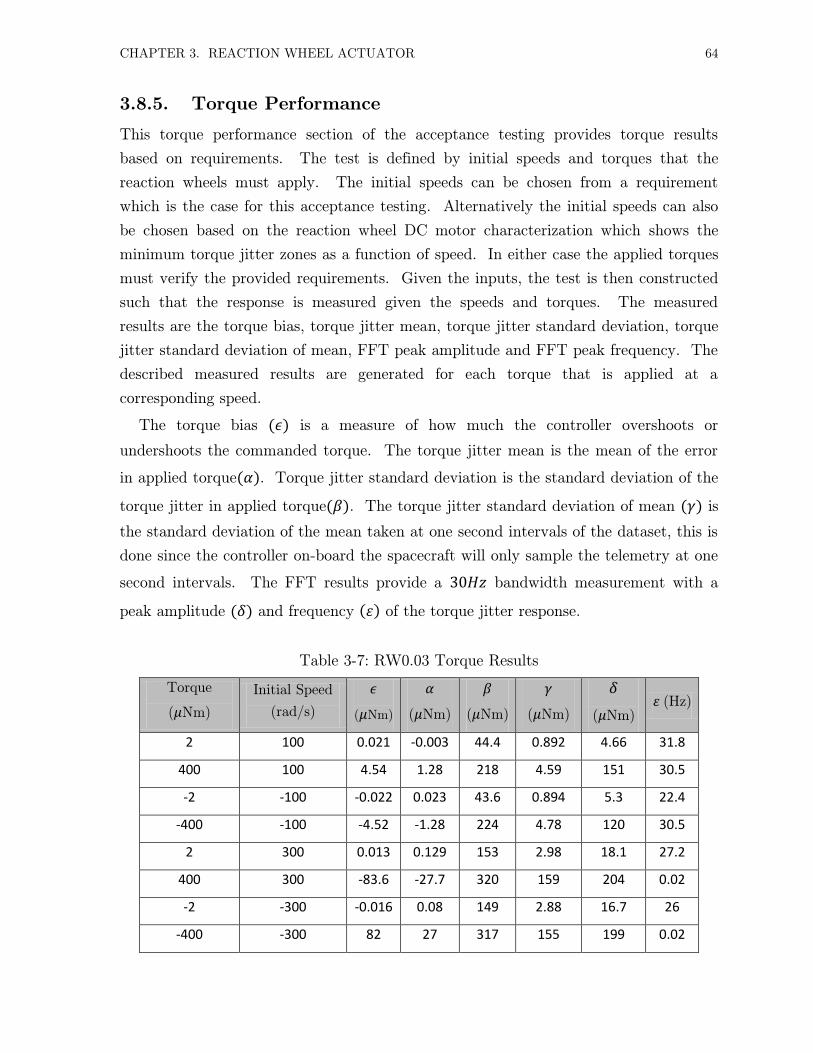
CHAPTER 3. REACTION WHEEL ACTUATOR 64
3.8.5. Torque Performance
This torque performance section of the acceptance testing provides torque results
based on requirements. The test is defined by initial speeds and torques that the
reaction wheels must apply. The initial speeds can be chosen from a requirement
which is the case for this acceptance testing. Alternatively the initial speeds can also
be chosen based on the reaction wheel DC motor characterization which shows the
minimum torque jitter zones as a function of speed. In either case the applied torques
must verify the provided requirements. Given the inputs, the test is then constructed
such that the response is measured given the speeds and torques. The measured
results are the torque bias, torque jitter mean, torque jitter standard deviation, torque
jitter standard deviation of mean, FFT peak amplitude and FFT peak frequency. The
described measured results are generated for each torque that is applied at a
corresponding speed.
The torque bias ( ) is a measure of how much the controller overshoots or
undershoots the commanded torque. The torque jitter mean is the mean of the error
in applied torque( ). Torque jitter standard deviation is the standard deviation of the
torque jitter in applied torque( ). The torque jitter standard deviation of mean ( ) is
the standard deviation of the mean taken at one second intervals of the dataset, this is
done since the controller on-board the spacecraft will only sample the telemetry at one
second intervals. The FFT results provide a bandwidth measurement with a
peak amplitude ( ) and frequency ( ) of the torque jitter response.
Table 3-7: RW0.03 Torque Results
Torque
( Nm)
Initial Speed
(rad/s)
( Nm)
( Nm)
( Nm)
( Nm)
( Nm) (Hz)
2 100 0.021 -0.003 44.4 0.892 4.66 31.8
400 100 4.54 1.28 218 4.59 151 30.5
-2 -100 -0.022 0.023 43.6 0.894 5.3 22.4
-400 -100 -4.52 -1.28 224 4.78 120 30.5
2 300 0.013 0.129 153 2.98 18.1 27.2
400 300 -83.6 -27.7 320 159 204 0.02
-2 -300 -0.016 0.08 149 2.88 16.7 26
-400 -300 82 27 317 155 199 0.02

CHAPTER 3. REACTION WHEEL ACTUATOR 65
Typical results are shown in Table 3-7 for the RW0.03 and Table 3-8 for the
RW0.06 reaction wheels. Both tables show the torque response of the reaction wheels
based on input speed and torque. Where for the RW0.03 reaction wheel the
requirement was set on the torque jitter standard deviation of mean ( ) to be less
than at an applied torque of and reaction wheel speed of
. For the RW0.06 reaction wheel the requirements were still being revised at the
time of writing this thesis and hence the results were based on the preliminary test
cases. The results did provide the torque jitter that can be obtained given the speed
of and with torques of and to be
acceptable.
Table 3-8: RW0.06 Torque Results
Torque
( Nm)
Initial Speed
(rad/s)
( Nm)
( Nm)
( Nm)
( Nm)
( Nm) (Hz)
10 50 0.214 0.554 121 10.1 27.7 3.23
60 50 1.18 0.562 129 8.3 23.2 3.83
-10 50 -0.186 0.222 95.7 11.4 27.7 2.49
-60 50 -1.15 0.509 68.3 14.7 17.8 0.56
10 300 0.172 0.437 283 9.51 27.7 26.3
60 300 1.15 0.358 276 6.63 27.3 30.4
-10 300 -0.221 0.021 281 6.58 30.6 22.6
-60 300 -1.19 -0.185 251 4.98 31.5 30.9
3.8.6. Operational Over Temperature
This part of the acceptance testing is composed of performing the nominal test and
torque performance test at defined operational temperatures. The temperature profile
is typically defined as the following temperature plateaus in sequence:
Room temperature
Hot temperature (Survival and Operational)
Cold temperature (Survival and Operational)
Cyclical between hot and cold temperature operational
Room temperature

CHAPTER 3. REACTION WHEEL ACTUATOR 66
The test is performed to ensure that the nominal and torque performance are not
significantly affected by temperature variations. All reaction wheels tested met the
requirements outlined earlier through the complete temperature profile.
3.9 Summary of Contribution
The RW0.03 and RW0.06 reaction wheels are high-performance active attitude control
actuators which are becoming more crucial for nanosatellite missions. Given the
pointing requirements for recent missions this is the only type of actuator available
that can provide fine pointing capability for the nanosatellite bus. The author’s
contribution with regard to this type of actuator was:
Reaction wheel DC motor analysis, verification and characterization
Communication interface characterization and verification
Analysis of regeneration impact on spacecraft power system
Reaction wheel safe operation due to regeneration
Design of acceptance test plan for reaction wheels
Detection of a current bias in RW0.03 reaction wheels
Reaction wheel enclosure and communication harness design and
implementation
Acceptance testing of reaction wheels with verification of requirements
3.9.1. Future Work
It is envisioned that the future acceptance testing of the reaction wheel actuator will
involve an external measurement of torque jitter. This is due to the current limitation
which pertains to the telemetry being only representative of the controller response
and not accounting for external sources of torque jitter. The reaction wheel torque
disturbances can be broken down into the following categories:
Mechanical disturbance
o Rotor and Cage mass imbalance
o Ball bearing sizing error
o Bearing misalignment

CHAPTER 3. REACTION WHEEL ACTUATOR 67
Control disturbance
o Constant speed
o Change in speed (Torque)
The current acceptance testing has provided a measure of the control disturbance as a
measurement of torque jitter. Below Figure 3-30 shows an alternative method of
measuring disturbances generated by the reaction wheel. This method consists of
mounting a reaction wheel on a fixture that through the use of load cells is capable of
resolving the generated reaction wheel disturbances in terms of torques and forces.
The main advantage of this method is that it provides an external spectral
measurement of the torques and forces generated by the reaction wheel. This type of
acceptance testing has been previously used on NASA’s Hubble Space Telescope
reaction wheels [24]. The challenges of this type of method are that initial calibration
is required to account for resonance and damping which can be difficult and time
consuming to determine.
Figure 3-30: External Disturbance Measurement [25]
The results from the external disturbance measurement are shown on a Power Spectral
Density plot (PSD). An example plot is shown in Figure 3-31, where the disturbance
is shown as a function of reaction wheel speed and frequency. The response on the
plot can provide insight into the following mechanical disturbance sources:
Radial Translation
o Rotor and cage mass imbalance
o Bearing misalignment
Radial Rocking
o Ball sizing error
o Bearing misalignment

CHAPTER 3. REACTION WHEEL ACTUATOR 68
Figure 3-31: Possible External Disturbance Results [25]
Using a single axis accelerometer and measuring the disturbance generated from a
RW0.03 reaction wheel has generated the results shown in Figure 3-32, which is an
uncompensated result. This means that the measurement is not calibrated for
resonance and damping.
Possible Radial
Translation
Figure 3-32: Power Spectrum Density Uncompensated Experimental Results

CHAPTER 3. REACTION WHEEL ACTUATOR 69
It can be suggested that the RW0.03 reaction wheel could have contributing
mechanical disturbance due to radial translation which could indicate a rotor and cage
mass imbalance and or bearing misalignment. It should be noted that the data was
obtained using an uncompensated test setup which does not validate the magnitudes
of the disturbance but does indicate that there could be external disturbances present.
The impact of these results on the spacecraft are that a reaction wheel acceptance
testing might not capture all contributing torque jitter sources and hence the torque
jitter obtained during acceptance testing may not be representative of the actual
torque jitter. In an effort to mediate this it can be further suggested that the
spacecraft should have a frequency based torque jitter requirement. This would aid in
only measuring disturbances at frequencies that can impact the spacecraft bus and
would also provide a complete external torque and force measurement of the reaction
wheel actuator.

70
Chapter 4
Passive Magnetic Actuator
The passive magnetic actuator described in this chapter is a hysteresis rod. This type
of actuator provides damping of spacecraft angular rotations which reduces the
angular momentum of a spacecraft. The removal of energy from the spacecraft is
possible due to a hysteresis effect of a ferromagnetic material. This chapter is broken
down into two sections: the design process and acceptance testing of hysteresis rods.
The design process is based on what was done for the Munin Nanosatellite [26] and the
Nanosatellite Tracking Ships (NTS) [27]. The hysteresis rod acceptance testing is
based on acceptance testing performed for the Munin Nanosatellite but adapted to
NTS type missions at the Space Flight Laboratory (SFL). This provides a generic
example of the design and testing of hysteresis rods for the Generic Nanosatellite Bus
(GNB) type of spacecraft.
4.1 Magnetic Hysteresis Background
In magnetic hysteresis there are a number of relationships that are used to describe
the overall behaviour of the material response or magnetic flux density to a
magnetic field strength input . The overall relationship is shown by the following
equation (4.1):
(4.1)
where
.

CHAPTER 4. PASSIVE MAGNETIC ACTUATOR 71
Where, is the magnetic permeability of a material and has a non-linear behaviour as
a function of or magnetic field strength input as shown in Figure 4-1, where the
nonlinear behaviour of magnetic permeability is shown.
Figure 4-1: Permeability of a Ferromagnetic Material
It is very important to realise that the magnetic field strength ( ) is the input into
the system and that the chosen medium provides the particular permeability ( ) which
yields a specific magnetic flux density ( ) or output. This is shown in Figure 4-2,
where a sample response for a material is plotted.
Figure 4-2: Magnetic Hysteresis Response
( )
( )

CHAPTER 4. PASSIVE MAGNETIC ACTUATOR 72
Explanation of key parameters that have been identified in Figure 4-2 are as follows:
is the coercive force, which is the minimum magnetic field strength input
needed to reduce the residual field to zero after input field is removed and
the material was at saturation
is the residual magnetic flux density after the input is removed
is the magnetic field strength needed to bring the material to saturation
is the maximum magnetic flux density that the material can maintain as a
function of input
∮ is the area under the curve which corresponds to the amount of energy
absorbed by the material through a hysteresis cycle
4.2 Design of Hysteresis Rods
The design process begins with a review of spacecraft that have utilized hysteresis rods
and leads into a top down/bottom up requirement driven design. The review of
previous spacecraft provides a baseline check of hysteresis rod parameters. The top
down requirements are a function of the type of orbit that the spacecraft will be in
and hence the magnetic field strength that the hysteresis rods will be saturated in.
The bottom up requirements are a function of maximizing the distance of the
hysteresis rods from an on-board permanent magnet, maintaining a perpendicular
orientation of the rods to the magnet and sizing the rods as a function of relative
position between the rods constrained by the spacecraft bus size.
The following Table 4-1 shows the spacecraft and hysteresis parameters that had
been considered for Nanosatellite Tracking Ships (NTS):
Table 4-1: Design Points for NTS Based on Mission Scaling [27]

CHAPTER 4. PASSIVE MAGNETIC ACTUATOR 73
The following Table 4-2 shows the spacecraft and hysteresis rod parameters that were
considered for the Munin spacecraft:
Table 4-2: Parameters of Hysteresis Rods of Various Satellites [26]
Hysteresis rod design captures the following parameters that affect the damping
produced by the hysteresis rods:
1. Material properties and heat treatment
2. Volume
3. Arrangement on spacecraft bus
4. Elongation (L/D)
4.2.1. Material Properties and Heat Treatment
As previously mentioned the top down requirement is typically the magnetic field
strength that the hysteresis rods would be exposed to. As an example for Munin the
field strength was estimated to be at the equator and up to at the
poles for a orbit. Based on this information a material selection was made
such that the coercive field is minimized while the area under the curve is
maximized. This provided for maximum damping given the availability of a material.
For an accurate estimate of the area under the curve the material would be tested
( curve) at the magnetic field strength expected on-orbit. Below are shown the
selections of materials for the Munin and NTS spacecraft.
Material properties that were chosen for NTS are shown in Table 4-3, showing a
Nickel-Iron alloy. This is the same material that had been previously used by the
Sapphire spacecraft shown in Table 4-1.

CHAPTER 4. PASSIVE MAGNETIC ACTUATOR 74
Table 4-3: Parameters of Nickel-Iron Alloy
Initial Magnetic
Permeability µin
Maximum Magnetic
Permeability µmax
Coercive Field Hc
(A/m)
Residual Flux Br
(T)
Saturation Flux
Density Bs (T)
Saturation Field Hs (A/m)
12100 124000 2.86 0.96 1.49 795.77
Material properties that were chosen for Munin are shown in Table 4-4, showing a
Molybdenum permalloy as the chosen material. The Munin spacecraft is of interest
for NTS since its bus size and performance metrics are similar.
Table 4-4: Parameters of Molybdenum Permalloy of the 79NM sort [26]
The material properties can be altered through a heat treatment process which may
improve the hysteresis response. Typically this is done in the form of annealing by the
supplier during the manufacturing process. Annealing is applied to the ferromagnetic
material in order to soften the material and reduce the saturation induction and
coercive force. This essentially produces a narrower hysteresis loop. If heat treatment
is applied to harden the material then comparably the hysteresis loop will be wider.
Materials should be tested in final configuration such that the desired hysteresis loop
is confirmed.
4.2.2. Volume of Hysteresis Rods
The following two equations provide the required volume of material that should be
present on-board the spacecraft such that a reduction of spin occurs in a define period
of time. The estimate does not compensate for magnetic dipole that could be present
on-board the spacecraft from other sources. Typically the performance will be lower
than the calculated estimate.

CHAPTER 4. PASSIVE MAGNETIC ACTUATOR 75
The relationship between spacecraft rotation and energy absorbed by spacecraft can be
defined by the following approximation (4.2):
(∮ ) (4.2)
Rewriting the above and introducing initial angular rotation we get equation (4.3):
( ) ( ) (∮ )
(4.3)
where ( ) The initial angular speed of spacecraft about an axis
( ) The final angular speed of spacecraft about an axis
The estimated volume of rod that will be used on the spacecraft
∮ The surface area on the B-H curve which can be estimated from a
mathematical model or actual measured B-H curve of material at the
expected magnetic field strength (H)
The magnetic flux density of the hysteresis rod at the magnetic field
strength input (H)
The required spin down time for the spacecraft about an axis.
The equation (4.4) can be rewritten providing the time it takes for the rotational
speed to be damped:
( )
(∮ ) (4.4)
It should be noted that a mathematical model developed by NASA (N95-27801) can be
used to predict the hysteresis curve [28]. This model was developed as a
function of the material data that was supplied to NASA and is an approximation to
that data (hysteresis curve). The inputs into the model are the parameters
shown in Figure 4-2. Sample output of this model can be seen in Figure 4-3.
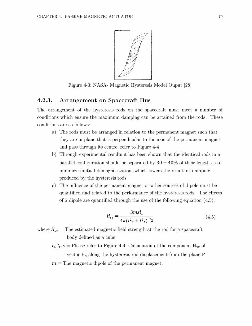
CHAPTER 4. PASSIVE MAGNETIC ACTUATOR 76
Figure 4-3: NASA- Magnetic Hysteresis Model Ouput [28]
4.2.3. Arrangement on Spacecraft Bus
The arrangement of the hysteresis rods on the spacecraft must meet a number of
conditions which ensure the maximum damping can be attained from the rods. These
conditions are as follows:
a) The rods must be arranged in relation to the permanent magnet such that
they are in plane that is perpendicular to the axis of the permanent magnet
and pass through its centre, refer to Figure 4-4
b) Through experimental results it has been shown that the identical rods in a
parallel configuration should be separated by of their length as to
minimize mutual demagnetization, which lowers the resultant damping
produced by the hysteresis rods
c) The influence of the permanent magnet or other sources of dipole must be
quantified and related to the performance of the hysteresis rods. The effects
of a dipole are quantified through the use of the following equation (4.5):
( ) ⁄ (4.5)
where The estimated magnetic field strength at the rod for a spacecraft
body defined as a cube
, , Please refer to Figure 4-4: Calculation of the component of
vector along the hysteresis rod displacement from the plane
The magnetic dipole of the permanent magnet.

CHAPTER 4. PASSIVE MAGNETIC ACTUATOR 77
Figure 4-4: Calculation of the component of vector along the hysteresis rod
displacement from the plane [26]
The arrangement of the hysteresis rods on the Munin spacecraft can be seen in Figure
4-4 with the generalized distribution and position is shown. The arrangement in the
NTS spacecraft can be seen in Figure 4-5.
Figure 4-5: NTS Attitude Subsystem Component Placement [27]
4.2.4. Elongation (L/D)
The geometry of the hysteresis rod is an iterative process between this Section 4.2.4
and Section 4.2.3. The rod size is constrained by the availability of space and
arrangement of rods on spacecraft. At this point of the design process the material
and volume for the hysteresis has already been determined in Sections 4.2.1 and 4.2.2.
Permanent Magnet
Hysteresis Rods

CHAPTER 4. PASSIVE MAGNETIC ACTUATOR 78
The typical optimal range for hysteresis rod elongation ( ) is . The
elongation that was used on NTS was and the elongation that was used on Munin
was . Coefficient of demagnetization can be determined through the following
approximation (4.6):
( )
(4.6)
where Demagnetization coefficient
Elongation parameter defined as length/diameter.
The magnetic permeability of the rod is dependent on the material permeability
through the following approximation (4.7):
( ) (4.7)
The above equation shows that the change in rod permeability as a function of
material permeability can be reduced by adjusting the elongation parameter. Since
the variation of rod material permeability ( ) as a function of its length is small, the
mean of the rod permeability ( ) can be used instead. This provides an
approximation of a constant permeability that can be used for a hysteresis rod.
4.2.5. Verification of Design
The verification of the hysteresis rod design process is divided into two phases. The
first phase is the simulation of the spin down performance. The second phase is the
simulation of steady state behaviour. Typically this can result in adjustments in
hysteresis rod design given the simulation results.
In more detail the spin down behaviour is simulated using the developed spacecraft
equations of motion which should capture the following hysteresis rod parameters:
Constant magnetic permeability derived in Section 4.2.4
Parasitic magnetic field strength that exists in spacecraft body from Section
4.2.3 c), also becomes the magnetic field bias that the rod will be exposed to
Magnetic field strength input from a geomagnetic field model

CHAPTER 4. PASSIVE MAGNETIC ACTUATOR 79
The steady state behaviour simulation shows the minimum response that the
hysteresis rods will provide in terms of damping. This simulation must account for the
following:
Constant magnetic permeability derived in Section 4.2.4
Parasitic magnetic field strength that exists in spacecraft body from Section
4.2.3 c), this provides an offset bias that the rods will be exposed to
Residual spacecraft rotation and the resultant change in field strength input
from a geomagnetic model
Comparison between the field strength input and coercive force of rod material
shows the limiting hysteresis loop which provides insight into the steady state
behaviour of the spacecraft
Magnetic field strength input from a geomagnetic field model
Hysteresis rods may go through further redesign pending on whether the results of this
section satisfy spacecraft top down requirements.
4.3 Hysteresis Rod Acceptance Testing
The current acceptance test plan of hysteresis rods consists of confirmation that the
hysteresis rods are showing a hysteresis phase lag and that a resultant magnetic field
flux is being generated as shown by a hysteresis response. This acceptance test is not
mission requirement driven. The phase lag is verified through the results shown in
Figure 4-6, showing the input signal and the lagging output signal which is a function
of the magnetic flux density generated by the hysteresis rod.
Figure 4-6: Hysteresis Phase Lag
INPUT HYSTERESIS
OUTPUT
PHASE LAG

CHAPTER 4. PASSIVE MAGNETIC ACTUATOR 80
The resultant magnetic field flux is then confirmed as a function of position along rod.
These results are shown in Figure 4-7, where a confirmation is made that the response
is similar from rod to rod and that the maximum response is in the middle of the rod
and minimum at the extremities.
Figure 4-7: Hysteresis Response - Position along Rod
4.3.1. Acceptance Testing - Test Fixture
The test fixture provides the capability of immersing the hysteresis rod in a chosen
magnetic field strength and then measuring the magnetic flux density through a
sensing coil. The fixture can be seen in Figure 4-8, where the use of Coil- is for the
magnetic field strength input and Coil- is a sensing coil for the magnetic flux density
feedback.
The operation of the fixture begins with insertion of the hysteresis rod into Coil- .
The magnetic field strength input to Coil- is then adjusted using the provided
potentiometers. During the adjustment process a multimeter can provide a measure of
the current to the coil which is directly proportional to the magnetic field strength
input.
The Coil- or sensing coil is then used to measure the magnetic flux density. The
coil provides its feedback in terms of voltage. The sensing coil can then be moved
across the length of the rod in Coil- to measure the voltage response as a function of
position along rod as described by Figure 4-7. The phase lag measurement is taken at
a particular position along rod and it is the lag between Coil- and Coil- signal.
Typically an oscilloscope is used to simultaneously display the voltage response and
0 15 30 45 60 75 90 105 120 135 1500.1
0.2
0.3
0.4
0.5
0.6
0.7
0.8
0.9
1
1.1
Position Along Rod (mm)
Peak-t
oP
eak V
oltage (
V)
Hysteresis Response
Origin of rod

CHAPTER 4. PASSIVE MAGNETIC ACTUATOR 81
phase lag during testing. Expected sensing voltage at a magnetic field strength is a
function of material properties and hysteresis rod design.
Figure 4-8: Hysteresis Rod Test Fixture
4.3.2. Acceptance Test Plan
As mentioned earlier the acceptance test plan is not mission requirement driven, it is
simply a verification of hysteresis response as a function of position along rod and
phase lag. The testing is comprised of setting a magnetic field strength input in
increments up to material saturation. A sample test plan is provided in Table 4-5.
Each test is broken down to voltage and phase lag measurements at positions along
rod. These positions are a function of rod length and sensing coil size.
Coil-2 Coil-1
Oscilloscope

CHAPTER 4. PASSIVE MAGNETIC ACTUATOR 82
Table 4-5: Hysteresis Rod Test Plan
HYSTERESIS ROD TEST PLAN
Test Vcoil-1 (VAC) icoil-1 (A) Hcoil-1 (A/m) Bcoil-1 (mT) Noise (VPk-Pk) Verified
A 0.3 0.0024 26.92 33.8 0.032 YES
B 0.5 0.0039 44.86 56.3 0.032 YES
C 1 0.0078 89.73 113 0.032 YES
D 2 0.0157 179.45 225 0.032 YES
E 5 0.0392 448.63 563 0.032 YES
F 10 0.0784 897.25 1130 0.032 YES
4.3.3. Acceptance Test Results
The acceptance test was completed for hysteresis rods using the described test
fixture. The expected result for sensing voltage at rod centre and material saturation
is at least , with a minimum at the extremities of the plot, while the phase lag
response was expected to be between to as the position along the rod
changes.
Figure 4-9: Phase Lag for Magnetic Field Strength

CHAPTER 4. PASSIVE MAGNETIC ACTUATOR 83
The result for phase lag of a rod at a magnetic field strength input of can be
seen in Figure 4-9. This is a valid response showing lag of the green wave
corresponding to Coil- behind the blue waveform which is Coil- . The irregularities
seen at the peaks of the green waveform are a function of nonlinearities and are
washed away as the input approaches material saturation. The following are some of
the sources of non-linearity:
Magnetic permeability
o Type of material
o As a function of magnetic field strength input
Geometry of rod
o Elongation (L≫D)
o Volume
Manufacturing process
o Heat treatment
o Cutting process
Figure 4-10: Hysteresis Response for Magnetic Field Strength
0.4
0.5
0.6
0.7
0.8
0.9
1
1.1
1.2
7.5 22.5 37.5 52.5 67.5 82.5 97.5 112.5 127.5 142.5
Pe
ak-t
o-P
eak
Vo
ltag
e (
VP
k-P
k)
Position Along Rod (mm)
Hysteresis Response
ADV
AE2
ADX
AE4
ADY
ADW
ADT
ADU
ADS
AE3
AE1
ADZ

CHAPTER 4. PASSIVE MAGNETIC ACTUATOR 84
The hysteresis response from sensing Coil- at a magnetic field strength input of
can be seen in Figure 4-10. The legend identifies the hysteresis rods being
tested with corresponding serial number names. Each plot on this Figure corresponds
to a particular hysteresis rod. This is a valid response with all hysteresis rods
showing a similar concave down response with a peak of just over . It is very
important to understand that hysteresis is a very complex behaviour which is
influenced by the non-linearities mentioned earlier. The response that is measured
here is not only the voltage but also the overall visual plot which must be concave
down and relatively similar between rods of the same design.
Figure 4-11: Phase Lag for for Magnetic Field Strength
The phase lag for a field strength input at material saturation is shown in Figure 4-11.
This result has shown the output (green) lagging behind input (blue) at a phase
difference of between to which makes it a valid result. The irregularities on
the output signal (green) are washed out due to the material being at magnetic field
strength saturation.

CHAPTER 4. PASSIVE MAGNETIC ACTUATOR 85
Again at saturation the hysteresis response for the rods is shown in Figure 4-12.
The results are valid with a concave down response and a centre peak voltage of at
least .
Figure 4-12: Hysteresis Response for Magnetic Field Strength
4.4 Summary of Contribution
The hysteresis rod exhibits very complex behaviour which requires iteration of design
to meet spacecraft requirements and careful interpretation of results during acceptance
testing. The author’s contribution is comprised of the following:
Outline of hysteresis rod design for a spacecraft bus
Hysteresis rod test fixture design and implementation
Acceptance test plan for hysteresis rods
Acceptance testing of hysteresis rods
4.5 Future Work
The current acceptance test plan only ensures that the hysteresis rods in question are
of a ferromagnetic material given the phase lag and hysteresis response as a function of
5
10
15
20
25
30
35
40
7.5 22.5 37.5 52.5 67.5 82.5 97.5 112.5 127.5 142.5
Pe
ak-t
o-P
eak
Vo
ltag
e (
VP
k-P
k)
Position Along Rod (mm)
Hysteresis Response ADV
AE2
ADX
AE4
ADY
ADW
ADT
ADU
ADS
AE3
AE1
ADZ

CHAPTER 4. PASSIVE MAGNETIC ACTUATOR 86
position along rod. A more complete analysis would be to generate the actual
plot as shown in Figure 4-2. The reason for this is as per equation (4.2) the energy
that is absorbed from the spacecraft is a function of the area under the curve.
Hence it would be beneficial to verify that the hysteresis rod curve meets the
minimum energy absorption requirement. It is important to understand that
variations in the plot can also be introduced from many sources including
during the manufacturing process as an example. These variations would not be
detectable using the current acceptance test plan. The developed test fixture can
generate a curve as shown on Figure 4-13, which can provide the energy
absorbed by the hysteresis rod. Work still needs to be completed in terms of
calibration of the hysteresis test fixture for the plot generation such that the
area under the curve has been validated.
Figure 4-13: B-H Plot for Hysteresis Rod

87
Chapter 5
Attitude Hardware Emulator
The purpose of the Attitude Hardware Emulator (AHE) is to replace the need for
spare attitude hardware which is a significant extra cost to nanosatellite missions.
This chapter describes the emulation of attitude hardware in software with emphasis
on the reaction wheel actuator and fine sun sensor. In order for the emulation to be
representative of actual hardware a number of requirements must be met. These
include major software states such as a bootloader and application mode. Finally the
emulator must be capable of running multiple instances of the emulated hardware
within a specified level of performance.
5.1 Requirements
The requirements for the Attitude Hardware Emulator are as follows:
[AHE-1] Software must use Nanosatellite Protocol (NSP) for emulated
hardware communication
[AHE-2] The emulated hardware must have two software states: a bootloader
and application state
[AHE-3] Each software state must use the hardware model as a source for NSP
device parameters
[AHE-4] Up to instances of an emulated hardware device must be able to
operate on the same serial interface
[AHE-5] Emulated device performance must be confirmed against experimental
results
[AHE-6] The emulator must be able to sustain communication performance of
from each instance of emulated hardware

CHAPTER 5. ATTITUDE HARDWARE EMULATOR 88
5.2 Nanosatellite Communication Protocol
The Nanosatellite Protocol (NSP) provides a standardized method for device
communication on-board the spacecraft. The devices which use this protocol could
consist of attitude hardware, payload and communication system just to name a few.
Two important aspects of this protocol are packet integrity and communication
topology, which ensure proper operation [29].
The packet integrity checks for the NSP protocol can be further broken down into
Cyclic-Redundancy Check (CRC) and KISS framing, where the CRC check provides
error detection within the data carried by the packet, and KISS framing is a method of
adding beginning and end frames to each packet such that the start and end of packet
can be detected. If a CRC error or missing KISS framing is detected then a typical
device with NSP implementation will not acknowledge the packet as good transmission
and may request the same packet again.
The communication topology that allows multiple devices to communicate on the
same bus uses the master-slave concept. This is not a new concept and has previously
been implemented in a number of standard communication technologies such as
RS485, RS232, CAN-Bus and SPI just to name a few. The concept works on the
principle where the master is the only device that can send requests or ‘speak’ on the
communication bus and the slave is one of many devices which will reply to a request
or only ‘speak’ when spoken to. Hence, only the master can initiate communications
at any time while all slave devices are listening. This ensures that the communication
state of all devices that are spoken to is passive in nature and will not inhibit the
operation of the master device. The Figure 5-1 shows a typical master/slave
configuration with the outlined portion that is the focus of the emulator.
Reaction Wheel 2
Attitude Determination
and Control Computer
(Master)
Fine Sun Sensor 2
Fine Sun Sensor 1
Reaction Wheel 1
Emulation Environment (Slave)
Figure 5-1: Hardware Emulation NSP Topology

CHAPTER 5. ATTITUDE HARDWARE EMULATOR 89
5.3 Software States
The attitude control and determination hardware is divided into two main categories
the sensors and actuators. Both types of hardware have two fundamental software
states the bootloader and application mode. In bootloader and using the NSP protocol
the hardware can provide basic functionality which includes activating the application
mode, loading new application code, checking parameters and reading and writing
directly to a memory address. The application mode which can only be invoked from
the bootloader mode provides complete device functionality. Hence, it is important for
the purposes of the attitude hardware emulator to distinguish between the two modes
and establish how these interact in the emulation environment.
5.3.1. Bootloader Mode
The bootloader mode is the most basic state that an attitude actuator or sensor can be
in. This mode is the only state that is automatically invoked post power up of device.
This basic state does provide the NSP based interface but without any device
functionality. The typical interface is limited to the following:
1. Using NSP as a communication protocol
2. Loading new application code
3. Reading and writing to specific memory locations in the device
4. Performing checks of the onboard microprocessor
5. Polling telemetry that was saved while the device was in application
mode
6. Limitation of not being able to operate the device without entering the
application mode
7. Invoking the application mode
The implementation of the bootloader in software for a particular device consisted of
items , and from above. This is since items , , and are used for
troubleshooting of the device which is not necessary in software emulation due to the
ability to view the state of the device through the emulator. It should be clarified at
this point that the emulation environment mimics the behaviour of the device for the
spacecraft FlatSat as discussed in Chapter 1, and does not provide exact emulation of
the device hardware which is not necessary.

CHAPTER 5. ATTITUDE HARDWARE EMULATOR 90
5.3.2. Application Mode
The application mode is the only mode that provides full device functionality which is
typically described in the Interface Control Document (ICD) for a particular device.
This mode can only be entered from the bootloader mode and upon an application
mode exit command it always returns to the bootloader mode. The device uses an
implementation of NSP protocol for all communication. For the hardware emulator
this means that the application mode must mimic the behaviour of the actual attitude
hardware in application mode.
The emulation of hardware while in application mode consists of two major items,
the NSP interface and the hardware model in software. The NSP interface
implementation in terms of the response of the device to commands is provided at a
high level, where the details of which can be obtained from the ICD for the device and
are beyond the scope of this chapter. The types of application mode commands that
are available are shown in Table 5-1.
Table 5-1: Device Mode Commands
Type of Command Typical Command Effect of Command Notes
Telecommand 0x00001000 send to
device
Device enters
application mode
Only works in
bootloader
mode
Mode Commands Mode: 0x16 with
value of 0.02
Commands a reaction
wheel to enter torque
control mode and apply
a positive torque of
0.02 Nm A list of
commands are
available in the
Interface
Control
Document
(ICD) for a
specific device
Parameter
Commands
Parameter: 0x14
with value of 0.1
Commands a change in
parameter 0x14 to a
new value of 0.1
Mode Telemetry 0x00
The reply from the
device contains the
current mode type and
value
Parameter
Telemetry 0x14
Returns the value that
is stored by parameter
0x14

CHAPTER 5. ATTITUDE HARDWARE EMULATOR 91
The reaction wheel and the fine sensor each have a variety of available commands in
each type of listed command category. The implementation of the NSP interface
accounts for the command categories but does not implement the details of the
number of available commands. This is accomplished by polling the commands
directly from the software model of the device.
5.4 Hardware Modelling
The attitude hardware that is modelled in software consists of the reaction wheel
actuator and the fine sun sensor. Both devices use a combination of a mathematical
model and a characterization map to provide an appropriate response of the device in
software.
5.4.1. Reaction Wheel Model
The reaction wheel actuator is modelled using mathematical relationships,
characterization map and a software integral control loop. Each is described in more
detail with emphasis on software implementation. The work in this section is based on
previous work described in Chapter 3, where the characterization of the reaction wheel
actuator is described.
The behaviour of the reaction wheel actuator is described by the equation (5.1),
where the net torque is a function of the duty cycle , internal torque and
opposing torque . The net torque is shown by:
(5.1)
The relationship of internal and opposing torque and motor parameters is described in
Chapter 3. The duty cycle pertains to the amount of voltage being applied to the
drive stages at a particular internal torque. In Chapter 3 this was assumed to be
constant since the reaction wheel was always commanded at a constant torque. In
this section, it is important to capture the variation in duty cycle since with variation
of spacecraft bus voltage the applied voltage at the windings will change and affect
reaction wheel performance as per equation (3.5), (3.6), (3.7) and (3.10) [19]. The
equation (5.2) uses the characterization map of the DC motor performance in Chapter
3 as a lookup table to derive the power, torque, speed, current and voltage limitations.
The stall torque is , is a value of for which the internal torque has a
maximum magnitude, is a speed based parameter as described in equation (5.2) as a

CHAPTER 5. ATTITUDE HARDWARE EMULATOR 92
function of duty cycle, is the angular speed of the motor and is the maximum
speed at zero torque of the motor. The stall torque is described by:
( )
(5.2)
The opposing friction component of the torque is described in equation (5.3). This
equation is similar to the equation (3.13), the only difference being the friction
component is being written in an explicit form. Where as an example for the RW0.06
reaction wheel the coulomb friction component is and the viscous friction
coefficient is ( ). The opposing friction torque is described by:
( ) (5.3)
In software the described equations provide the method of coupling the integral control
loop and the characterization map. For a given requested angular acceleration and
assuming a rotor mass moment of inertia the software assumes that a torque is being
requested. This torque is then propagated forward in time using an integral loop
which is limited by the characterization map of the device. The map provides the
torque, speed, voltage, current and disturbance limitations that are imposed on the
integral control loop. This is accomplished by not only limiting the behaviour of the
loop but also injecting the disturbances into the loop. These could be poor speed
estimates, voltage changes due to bus voltage variation or other parameters which are
captured by the characterization map. A high level block diagram of the implemented
control behaviour between mathematical model, characterization and integral loop can
be seen in Figure 5-2.
Requested
Setpoint (NSP) Integral
Controller
Feedback from
Operating Point on
Characterization Map
Feedback
Gain Adjustment
Output Process
Variable (NSP)
External disturbances
such as bus voltage
Figure 5-2: Block Diagram of Reaction Wheel Model in Software

CHAPTER 5. ATTITUDE HARDWARE EMULATOR 93
5.4.2. Fine Sun Sensor Model
The fine sun sensor is a device that is part of the attitude determination system on
board the spacecraft. It is capable of providing spacecraft orientation in reference to
the sun line. The sensor is limited to a two dimensional solution and is unable to
provide the orientation of the spacecraft about the sun line. The device uses a
complementary metal-oxide-semiconductor array (CMOS) for sensing the sun line and
a microcontroller for post processing the data and detecting the centre of the ellipsoid
generated by the sun line on the CMOS [30]. The modelling of the device is
accomplished using a combination of the processing code that is used on-board the
sensor to mimic the centre of ellipsoid determination and the characterization map
which provides the CMOS response as a function of sensor orientation with respect to
the sun line. Figure 5-3 provides a summary of the model.
The model works on the foundation described in Section 5.3 where the NSP protocol is
used as the interface to the model. Given an NSP request the model will poll an
external sun line reference to determine where on the CMOS the ellipsoid will be
generated. The cross referencing of the sun line orientation with respect to the sensor
and the characterization map are both generated during acceptance testing of the
device and are beyond the scope of this thesis [30]. Figure 5-4 represents the generated
characterization of the sensor CMOS at angles of incidence to the sun line. Pointing
accuracy is shown as a variation of colour from red (low accuracy) to blue (high
accuracy). This map is used as a look-up table for a given sun line reference where the
accuracy and ellipsoid position are determined. The centre of the ellipsoid is then
calculated using the method employed on the sensor. Finally the output solution is
sent as a reply to the original NSP request.
External reference
for sun line Requested
Solution
(NSP) Fine Sun Sensor
Characterization Map
Centre of Ellipsoid
Detection on CMOS
Output
Solution
(NSP)
Figure 5-3: Block Diagram of Fine Sun Sensor Model in Software

CHAPTER 5. ATTITUDE HARDWARE EMULATOR 94
Figure 5-4: Fine Sun Sensor Characterization Map
5.5 Emulator Performance
At the time of writing this thesis the attitude hardware emulator performance had
only been verified for the NSP Section 5.3 software states and not the hardware
models in software. The verification of the NSP protocol entailed CRC, KISS and
packets per second tests. The results of which had verified requirements AHE-1,
AHE-2, AHE-3 and AHE-6. The detailed verification of these requirements was
accomplished through the implementation of the sections described earlier in this
chapter. The critical requirement AHE-4 and AHE-5 which ensures that the emulated
hardware behaviour has been confirmed against experimental results had not been
verified at the time of writing this thesis.
5.6 System Overview
The complete system topology is comprised of the attitude determination and control
computer, external reference source containing items common to all systems involved
such as orbit data and attitude hardware emulator and the emulator environment.
The Figure 5-5 shows a high-level overview of the system.

CHAPTER 5. ATTITUDE HARDWARE EMULATOR 95
Figure 5-5: Simplified Attitude Hardware Emulator Block Diagram
NSP
Orbit data B
us
Volt
age,
Sun lin
e re
fere
nce
,
Dis
turb
ance
s to
and fro
m d
evic
e
Hardware
Interface
Attitude Hardware Emulator PC
Attitude Determination and
Control Computer
NSP Request
Orbit
Propagator/
Spacecraft
System
Status
Reaction
Wheel X
Reaction
Wheel Y
Reaction
Wheel Z
Fine Sun
Sensor +X
Fine Sun
Sensor -X
Fine Sun
Sensor +Y
Fine Sun
Sensor -Y
Fine Sun
Sensor +Z
Fine Sun
Sensor -Z
Software Thread
Wheel Model
Software Thread
FSS Model
FlatSat Environment

CHAPTER 5. ATTITUDE HARDWARE EMULATOR 96
5.7 Future Work
The work on the attitude hardware emulator thus far has verified all requirements
except for the verification of model performance and operating multiple instances of
the hardware models at an appropriate communication performance. It is foreseen
that once the final requirements are verified this type of emulation environment will be
extended to other attitude hardware. Other hardware may include magnetorquers,
hysteresis rods, rate sensors, magnetometers and star trackers. This would provide for
a complete emulation environment for a FlatSat setup as discussed in Chapter 1.

97
Chapter 6
Conclusions
This thesis has detailed the analysis, verification and emulation of attitude hardware
for a nanosatellite scale of spacecraft. The characterization of attitude control
hardware has been completed through detailed analysis and verification of
performance. The results of which have been incorporated into acceptance test plans
that inherently build on heritage. The test plans had been used in verification of the
attitude control system requirements, which showed acceptable performance for all
hardware tested. The data obtained during testing further provided input into
software models which were implemented in the attitude hardware emulator. At the
time of writing this thesis a number of spacecraft missions await launch that
incorporated the work described herein.
The attitude control hardware that had been characterized included the reaction
wheel and hysteresis rods. The characterization came as a consequence of more
stringent requirements to which some of the devices had not been previously tested to.
Hence, the characterization provided for a performance map of the device beyond
previously tested limits. The performance had initially been established using
theoretical assumptions overlaid with previously collected data, which was verified
through careful testing. Both actuators acceptance tests had been modified providing
an overall improvement.
The reaction wheel actuator was characterized using a single phase DC motor
model with a friction model that was based on past run down data. This led to a
number of discoveries when the theoretical performance prediction was confirmed
experimentally. These included regenerative zones, high torque jitter zones and large
torque overshoot in zero crossings both for the RW0.03 and RW0.06 reaction wheels.

CHAPTER 6. CONCLUSIONS 98
The regenerative behaviour was mitigated through the use of a dummy load resistor
for acceptance testing and it was also verified that the spacecraft power system can
handle the regeneration. Two software changes had been requested, first to remove or
modify the software regenerative control as to reduce the torque jitter in regenerative
zones and second to develop a better speed estimator at zero crossing to minimize
torque overshoot. Overall the characterization map provided areas of best
performance based on which the acceptance testing was revised such that the
requirements were met. In total reaction wheels were tested meeting requirements.
The testing exhibited inherent limitations which were due to taking measurements
that were internal to the device and not actually measuring the physical torque jitter
output of the device which is the next logical step in future testing.
The hysteresis rod acceptance testing had not been previously established at the
Space Flight Laboratory. Hence the work completed was a design process for
hysteresis rods in order to develop an acceptance test such that the necessary
requirements are captured. As per requirements and due to flight heritage the
acceptance test had to meet two criteria which included the voltage response as a
function of the length of the rod and phase lag. In total hysteresis rods were tested
and verified against the requirements. The testing also showed that future
improvements could be made mapping out the curve for the rod using the
developed test fixture. This could provide for an estimate of the amount of energy the
hysteresis rod would absorb from one cycle.
The test results from characterization of the reaction wheel and a fine sun sensor
had been used to develop emulation of these devices in software. This is in an effort
to reduce cost and provide an invaluable resource for ground testing. For both devices
the characterization maps were used from acceptance testing in conjunction with
mathematical models that pertained to the specific performance behaviours. At the
time of writing this thesis some of the requirements had been verified and some were
left to be verified at the completion of the emulation software.
The work presented in this thesis has provided an in-depth insight into the
behaviour of attitude control hardware, acceptance testing and software emulation.
The linkage to how crucial this is for the success of nanosatellite scale spacecraft is
obvious as presented in this thesis. Given the growing demand for these types of
missions this is an area of ongoing development and research which ensures present
and future mission success.

99
Bibliography
[1] Herbert J. Kramer and Arthur P. Cracknell, “An overview of small satellites in
remote sensing," University of Dundee, Dundee, 2008.
[2] Najmus. Ibrahim, “NEMO-AM Attitude Determination and Control Subsystem
Design and Analysis," University of Toronto Institute for Aerospace Studies,
Toronto, 2011.
[3] Jesse K. Eyer, Benoit P. Larouche, Robert E. Zee. Nathan G. Orr, “Precision
Formation Flight: The CanX-4 and 5 dual Nanosatellite Mission," University of
Toronto Institute for Aerospace Studies - Space Flight Laboratory, Toronto, 2008.
[4] W. W. Weiss, A.F.J. Moffat, R.E. Zee, S.M. Rucinski, S.W. Mochnacki, J.M.
Matthews, M. Breger, R. Kuschnig, O. Koudelka, P. Orleanski, A. Pamyatnykh,
A. Pigulski, C.C. Grant. A. Schwarzenberg-Czerny, “The BRITE Nano-Satellite
Constellation Mission," Committee on Space Research, France, 2010.
[5] Pawel. Lukaszynski, “Research Assessment Committee Report #1," University of
Toronto Institute for Aerospace Studies, Toronto, 2011.
[6] Larson J. Wiley Wertz R. James, Space Mission Analysis and Design, 3rd ed. New
York, United States of America: Microcosm Press Inc., 2007.
[7] Michael Greene, “The Attitude Determination and Control System of the Generic
Nanosatellite Bus," University of Toronto Institute for Aerospace Studies,
Toronto, 2009.
[8] Bryan Johnson-Lemke, “High Performance Attitude Determination and Control
for Nanosatellite Missions," University of Toronto Institute for Aerospace Studies,
Toronto, 2011.
[9] Karan. Sarda, “Test Plan, Procedure and Results Report on Wheels," University
of Toronto Institute of Aerospace Studies, Toronto, 2008.

BIBLIOGRAPHY 100
[10] Christopher J. McNutt, “Modular Nanosatellites – Plug-and-Play (PnP)
CubeSat," Air Force Research Laboratory, Kirtland, 2009.
[11] Sven. Krischke, Manfred. Lemke, Norbert. Muncheberg, “Nanosatellites and Micro
Systems Technology – Capabilities Limitations and Applciations," Kayser-Threde
GmbH, Munich, 1996.
[12] Pascale Ehrenfreund, Antonio J. Ricco, Henry Hertzfeld. Kirk Woellert, “Cubesats:
Cost-effective science and technology platforms for emerging and developing
nations," Space Policy Institute - The George Washington University,
Washington, 2010.
[13] Ke Gong, Di Yang, Junfeng Li. Bingquan Wang, “Fine attitude control by
reaction wheels using variable-structure controller," Aerospace Technology Center
and Department of Electronic Engineering, Tsinghua University, China, 2003.
[14] F. Landis Markley, “Maximum Torque and Momentum Envelopes for Reaction-
Wheel Arrays," NASA Goddard Space Flight Center, Greenbelt, Maryland, 2010.
[15] Oh. Dong-Ik, Cheon. Hwa-Suk, “Precision Measurements of Reaction Wheel
Disturbances with Frequency Compensation Process," School of Aerospace and
Mechanical Engineering, Hankuk Aviation University, Hwajun, 2005.
[16] C. M. LIAW. M. C. CHOU, “Robust Current and Torque Controls for PMSM
Driven Satellite Reaction Wheel," National Tsing Hua University, 2009.
[17] Sinclair Interplanetary(Canada), “NSP Appication Software for Reaction Wheels.,"
Sinclair Interplanetary, Toronto, 2008.
[18] Peter C. Hughes, Spacecraft Attitude Dynamics. US: Dover Publications, 2004.
[19] Wertz R. James, Spacecraft Attitude Determination and Control. Boston, London:
Kluwer Academic Publishers, 2002.
[20] French R. James Griffin D. Michael, Space Vehicle Design , Second Edition ed.
Reston, United States : American Institute of Aeronautics and Astronautics Inc.,
2004.
[21] Dr. Duane Hanselman, Brushless Motors: Magnetic Design, Performance, and
Control. Orono: E-Man Press LLC, 2012.
[22] Electro-Craft Corporation, DC Motors Speed Controls Servo Systems. New Jersey:
Electro-Craft Corporation, 1978.

BIBLIOGRAPHY 101
[23] Bonin Grant, “Power System Design, Analysis, and Power Electronics
Implementation," University of Toronto Institute for Aerospace Studies, Toronto,
Thesis 2009.
[24] Pawel Lukaszynski, “Research Assessment Committee Report #2," University of
Toronto Institute for Aerospace Studies, Toronto, 2012.
[25] Shigemune. Ohkami, Yoshiaki. Tasniwaki, “Experimental and Numerical Analysis
of Reaction Wheel Disturbances," JSME International Journal, vol. 46, no. 2,
2003.
[26] M. Yu. Ovchinnikov and Penkov V. I., “Passive Magnetic Attitude Control
System for the Munin Nanosatellite," Cosmic Research, vol. 40, no. 2, pp. 156-170,
2002.
[27] S. Eagleson, “NTS Attitude Subsystem Design Document," University of Toronto
Institute for Aerospace Studies, Toronto, 2007.
[28] Thomas W. Flatley and Debra A. Henretty, “A Magnetic Hysteresis Model,"
NASA, Greenbelt, MD, 1995.
[29] Daniel D. Kekez, “Nanosatellite Protocol (NSP)," University of Toronto Institute
for Aerospace Studies, Toronto, Design Document SFL-GNB-OBC-D001, 2012.
[30] Karan. Sarda, “Test Plan, Procedure and Results Report on Sun Sensors,"
University of Toronto Institute of Aerospace Studies , Toronto, 2008.
[31] Sainz L., Corcoles F. Pedra J., “Harmonic Modeling of Induction Motors.,"
Department of Electrical Engineering, Barcelona, Spain, 2005.


![Libraries] Function of Attitude Similarity and Attitude](https://img.pdfslide.net/doc/110x75/62e4a200fe037104c8733690/libraries-function-of-attitude-similarity-and-attitude-.jpg)