ATTRIBUTE np CONTROL CHARTS USING RESAMPLING …

O P E R A T I O N S R E S E A R C H A N D D E C I S I O N S No. 2 2020 DOI: 10.37190/ord200207

ATTRIBUTE np CONTROL CHARTS USING RESAMPLING SYSTEMS FOR MONITORING

NON-CONFORMING ITEMS UNDER EXPONENTIATED HALF-LOGISTIC DISTRIBUTION

AMMARA TANVEER1, MUHAMMAD AZAM2, MUHAMMAD ASLAM3∗, MUHAMMAD SHUJAAT NAWAZ4

1National College of Business Administration and Economics, Lahore 54660, Pakistan 2Department of Statistics and Computer Science, University of Veterinary and Animal Sciences,

Lahore 54000, Pakistan 3Department of Statistics, Faculty of Science, King Abdulaziz University, Jeddah 21551, Saudi Arabia

4Higher Education Department, Government of the Punjab, Lahore 54000, Pakistan

An attribute np control chart has been designed using resampling systems for monitoring non- -conforming items under exponentiated half-logistic distribution. We suppose that lifetime follows ex-ponentiated half-logistic distribution. For the proposed control charts, the optimal parameters and con-trol limits have been obtained. The operational formulas for in-control and out of control average run lengths (ARLs) have been derived. Control constants are established by considering the target in-control ARL at a normal process. The extensive ARL tables are reported for various parameters and shifted values of process parameters. The performance of the proposed control chart is evaluated with several existing charts with regard to ARLs, which empower the presented chart and prove far better for timely detection of assignable causes. A wide range of tables, a real-life example, and simulation study for RGS and MDS are given for a better understanding of the problem.

Keywords: attribute chart, time truncation, process, statistical distributions, sampling schemes

1. Introduction

Quality is the main important feature for production growth and standing. Statistical techniques can be used to improve the quality of the product. The control chart is the

_________________________ ∗Corresponding author, e-mail address: [email protected] Received 5 November 2019, accepted 18 August 2020

A. TANVEER et al. 116

primary instrument to monitor the process and to finally develop high-quality products. Control charts provide a fast signal when the process is out of control. The control chart enables to monitor the deviation of the method over time and discovers the foundation for differences. Amongst the two types of control charts, i.e., attribute control charts and variable control charts, the former is used to track the quality characteristic of an attrib-ute. Examples of attribute control charts include p, np, and u control charts. The variable control charts, e.g., X, R, and S control charts are used to monitor the characteristics of the issue in question. For the construction of control charts, different schemes, e.g., sin-gle sampling scheme, double sampling scheme, repetitive group sampling scheme, and multiple dependent state sampling (MDS) schemes are used.

Repetitive group sampling (RGS) scheme is introduced by Sherman [1]. RGS is the expansion of a single sampling scheme. The control chart under RGS has two pairs of control limits. If a point lies within the inner control limits, the procedure is said to be in-control, whereas if a point lies beyond the outer control limits, the process is out of control. The sampling is repeated if a point is identified between inner and outer control limits until a decision is made. Balamurali and Jun [2] introduce the RGS plan for vari-able inspection. They reveal that the average sample number (ASN) of the RGS plan is lesser than both single and double sampling plans. Ahmad et al. [3] Design the X con-trol chart for RGS based on the process capability index. Aslam et al. [4], using RGS, present attributes and variables control charts. Aslam et al. [5] introduce a t-chart using RGS. Rao [6] introduces a control chart based on exponentiated half logistic distribution with known shape parameters. The wide range of tables based on a simulated study is given.

Multiple dependent state (MDS) sampling scheme was created by Wortham and Baker [7]. The conclusion will be made not only on current but also on a previous or upcoming lot. The plan parameters are established by meeting the vendor and customer hazards at a number of acceptable levels of quality and by restricting the amount of quality. Later, Aslam et al. [8] propose a new loss consideration process under multiple dependent state variable sampling plans. Aslam et al. [9] propose multiple dependent state control chart based on two pairs of control limits. The proposed control chart is compared with the existing X chart which shows that the proposed control chart per-forms better than Shewart X bar control chart. Rao and Naidu [10] Recommend a fresh sampling plan for exponentiated half logistic distribution for group acceptance. The scheme implemented by them shows that the percentile ratio rises for all parameters and decreases the number of associations. Aslam [11] proposes a control chart by using the Weibull distribution based on MDS sampling which is more efficient than the existing control charts.

In this study, an attribute np control chart for process monitoring using exponenti-ated half logistic distribution (EHLD) is provided as based on RGS and MDS. Both of the control charts are compared with the existing control charts.

Attribute np control charts using resampling systems 117

RGS chart is compared with the existing chart on the basis of exponentiated half logistic distribution provided by Jeyadurga et al. [12]. We acquire optimal parameters, control limits, and also show the respective ARL and ASN values of the control chart using RGS. We compare the table values for the shape parameters α = 2 and 3 and the specified ARL is r0 = 300 and 370, respectively. We can infer from our data that the proposed chart identifies the process shift quicker than the existing chart under RGS sampling scheme. The control chart performance in RGS is also compared with the con-trol chart presented by Rao [6] based on EHLD. Results are presented in form of tables using different shape and scale parameters, respectively.

The efficiency of the proposed MDS control chart is compared to the control chart results by Aslam [11]. We calculate the optimal parameters, control limits, and present the respective ARL values of the control chart, using dependent state sampling. The re-sults are shown in the form of a table which indicates that the proposed control chart is more responsive than the existing control chart to recognize a shift in the process. The efficiency of the proposed MDS control chart is also compared with the results of Rao [6] and concluded in the form of tables, using different ARL0 (200, 300, 370, i = 1, 2, 3).

Moreover, using RGS and MDS, we find the ARLs when scale and shape parameters are shifted separately, and also when both parameters are shifted at once. A real-life data example is also used to demonstrate the proposed np control chart by using simu-lated data.

2. The exponentiated half-logistic distribution (EHLD)

EHLD is a simplification of half-logistic distribution proposed by Mudholkar and Srivastava [13]. Cordeiro et al. [14] study mathematical properties of the exponentiated half logistic family of distributions. Seo and Kang [15] derive moment estimators and maximum likelihood estimators of unknown parameters of exponentiated half logistic distribution along with an entropy. Elgarhy et al. [16] present exponentiated extended family of distributions along with its mathematical properties and applications. Usman et al. [17] study the Kumaraswamy half-logistic distribution and explore the properties and applications of the presented model. Anwar and Bibi [18] propose half logistic gen-eralized Weibull (HLGW) distribution and investigate its properties.

The cumulative distribution function (F(t) and the probability density function ( f(t) of EHLD are given as

( )/

/1 e , 0,1 e

t

tF t tασ

σ α σ−

−

−= ≥ > 0, > 0 + (1)


( ) ( )( )/ /

/

2 e 1 e, 0, 0, 0

1 e

t t

tf t t

ασ σ

ασ

αα σ

σ

−1− −

+1−

−= ≥ > >

+ (2)

Here α is the shape parameter, and σ is the scale parameter. The arithmetic mean of EHLD distribution is specified as

1/ 1/

1/ 1/1 0.5 1 0.5ln , ln , ,1 0.5 1 0.5

α α

α αμμ σ η μ ση ση

+ += = = = − − (3)

3. Design of the proposed control chart under RGS

It is important to note that the attribute’s RGS plan is a generalization of the ordinary single sampling plan. In RGS, the sampling is repeated until a decision is made. RGS is more efficient than the single sampling in terms of the ASN which is needed for decid-ing on the disposition of the lot.

Following are the steps of the np control chart based on the RGS scheme.

Step 1. From the manufacturing process, choose a subgroup as a random sample of size n and place it on the life test for the particular time t0. Count number of failures says D during t0.

Step 2. If LCL1 ≤ D ≤ UCL1, then the process is said to be in control. If either D ≥ UCL2, or D ≤ LCL2, then the process is said to be out of control.

Step 3. Repeat Steps 1 and 2 if LCL2 < D < LCL1 or UCL1 < D < UCL2, until a decision is made.

The control limits for an np control chart are as follows:

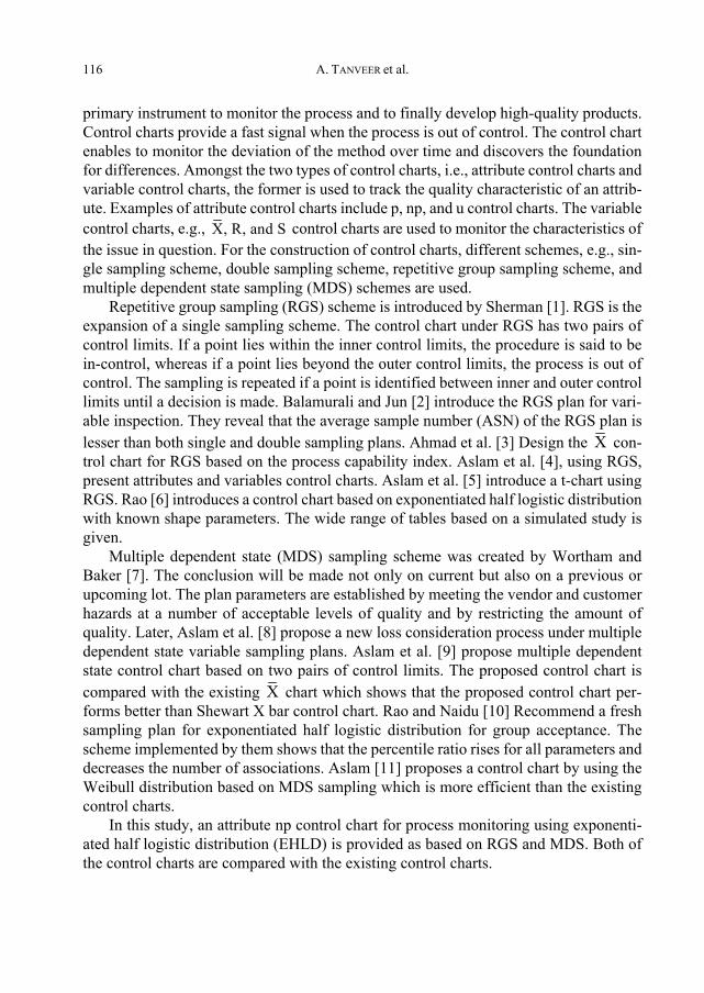
( )1 0 1 0 01UCL np k np p= + − (4a)

( )( )1 0 1 0 0max 0, 1LCL np k np p= − − (4b)

( )2 0 2 0 01UCL np k np p= + − (4c)

( )( )2 0 2 0 0max 0, 1LCL np k np p= − − (4d)

The likelihood p0 is generally unknown. So, the control limits to be used in practical applications will be as given by [19]:


1 1 1 dUCL d k dn

= + −

(5a)

1 1max 0, 1 dLCL d k dn

= − − (5b)

2 2 1 dUCL d k dn

= + −

(5c)

2 2max 0, 1 dLCL d k dn

= − − (5d)

where d is the average number of failures in a subgroup over a preliminary sample. However, in this paper, we will consider the control limits in the form of equation (4) to investigate the performance of the proposed chart analytically in terms of the average run length.

The method is stated to be controlled if t = αμ0, μ = μ0 (scale parameter is σ = σ0

and shape parameter is α = α0). If the process is in control, the failure likelihood p0 is given by equation (1)

00 0

0 0

0 00 0 0 0

0 0 0 0

//

0 //

/

/

1 e 1 e,1 e 1 e

1 e 1 e1 e 1 e

at

at

a a

a a

p pαα μ σσ

μ σσ

α ασ η σ η

σ η σ η

−−

−−

− −

− −

− −= = + +

− −= = + +

(6)

3.1. Shift in the scale parameter

We suppose that the scale parameter is shifted from σ0 to σ1 = cσ0, where c is a shift constant (or scale parameter is σ = σ1). So, if the process is out of control, the failure likelihood of an item p1 is specified as


0 1

0 1

0 0 0 0

0 0 0 0

//

1 //

/c /

/c /

1 e 1 e,1 e 1 e

1 e 1 e1 e 1 e

t

t

a a c

a a c

p pαα αμ σσ

αμ σσ

α ασ η σ η

σ η σ η

−−

−−

− −

− −

− −= = + +

− −= = + +

(7)

3.2. Shift in shape and both shape and scale parameters

If shape parameter is shifted from α0 to α1 = fα0 (or the shape parameter is α = α1). The probability that an item is failed p2 is specified as

0 01

01

1/

2 1 1/1 e 1 0.5where ln1 e 1 0.5

f fa

fapα αη

αη η−

−

− += = + − (8)

Suppose that both the shape and scale parameters are shifted to α1 = fa0 and σ1 = cσ0 (now the shape parameter is α1 and the scale parameter is σ1). The likelihood that an item is failed p3 is specified as

0 01

01

1//

3 1 1//1 e 1 0.5where ln1 e 1 0.5

fa fa c

fa cpαη

αη η−

−

− += = + − (9)

When the probability that the process is likely to be in-control, L1(p) is specified as

( ) ( )

( )[ ]

[ ]( )

1

1

1 1 1

11

, 0,1, 2, ...,

1 , 0,1, 2, ...,UCL

n dd

d LCL

L p P LCL d UCL d n

nL p p p d n

d−

= +

= ≤ ≤ =

= − =

(10)

Similarly, when the process is likely to be stated out of control, L2(p) is specified as

( ) ( ) ( )

( ) ( )[ ]

[ ]2

2

2 2 2

21

1LCL

n dd

d UCL

L p P d UCL P d LCL

nL p p p

d−

= +

= > + <

= −

(11)

The likelihood of repeating the sampling until the choice is made, L3(p) is as illus-trated

( ) ( ) ( )

( )[ ]

[ ]( )

[ ]

[ ]( )

1 2

2 1

3 2 1 1 2

31 1

1 1LCL UCL

n d n dd d

d LCL d UCL

L p P LCL d LCL P UCL d UCL

n nL p p p p p

d d− −

= + = +

= ≤ < + ≤ <

= − + −

(12)


The likelihood that the process will be controlled the ASN and average run length (ARL) using RGS are given below:

( ) ( )( )

1

3in

L pp p

L p=

− (13)

( ) ( )31nASN p

L p=

− (14)

( )

11 in

ARLp p

=−

(15)

The likelihood that the process will be controlled when it is under control using RGS, the scale parameter is shifted, shape parameter is shifted and both shape and scale parameters are shifted is given in equations (13a)–(13d), respectively:

( ) ( )( )

1 00

3 01in

L pp p

L p=

− (13a)

( ) ( )( )

1 11

3 11in

L pp p

L p=

− (13b)

( ) ( )( )

1 22

3 21in

L pp p

L p=

− (13c)

( ) ( )( )

1 33

3 31in

L pp p

L p=

− (13d)

The ASN for the proposed chart when the process is in control, the scale parameter is shifted, the shape parameter is shifted and both scale and shape parameters are shifted is given in equation (14a)–(14d), respectively:

( ) ( )03 01nASN p

L p=

− (14a)

( ) ( )13 11nASN p

L p=

− (14b)

( ) ( )23 21nASN p

L p=

− (14c)


( ) ( )33 31nASN p

L p=

− (14d)

The ARL for the proposed chart when the process is in control, the scale parameter is shifted, the shape parameter is shifted and both scale and shape parameters are shifted is given in equation (15a)–(15d), respectively:

( )0

0

11 in

ARLp p

=−

(15a)

( )1

1

11 in

ARLp p

=−

(15b)

( )2

2

11 in

ARLp p

=−

(15c)

( )3

3

11 in

ARLp p

=−

(15d)

3.3. Optimization conditions

The following are the optimization conditions:

Minimize ASN(p0)

Subject to

ARL0 ≥ r0

k2 > k1

Algorithm Step 1. Set the values of α0 (shape parameter), a (test termination ratio), r0 (in-con-

trol target ARL), and set a greatest value for ASN as ASNm. Step 2. Set the values of n, k1 and k2. Step 3. Put the values of a, α0 in equation (6) to find the failure probability (p0). Step 4. Discover the control limits of the proposed control chart using the values of

n, p0, k1, and k2 in equations (4a)–(4d). Step 5. Find the likelihood that the process will be declared in-control when the

process is in-control by replacing the values of p0 and control limits in equations (10), (12), and (13a); also use the equation (15a) to locate ARL0. By using equation (14a), compute the ASN at p0.


Step 6. Check parameters n, k1 and k2 such that the in-control ARL0 is as near as to the final value r0. Make the comparison of ASN(p0) value with ASNm. If ASN(p0) ≤ ASNm, then set ASNm = ASN(p0).

Step 7. Continue Steps 4–6 for various combinations of n, k1 and k2 until you get an ARL0 as near as to r0 and obtain the least value of ASN as ASNm.

Step 8. Replace the values n, k1 and k2 in equations (7)–(9), (13b)–(13d), (15b)–(15d) for discovering the out of control ARL1 for various shift values. Use equations (14b)–(14d) to discover the respective ASNs.

3.4. Control charts performance comparison

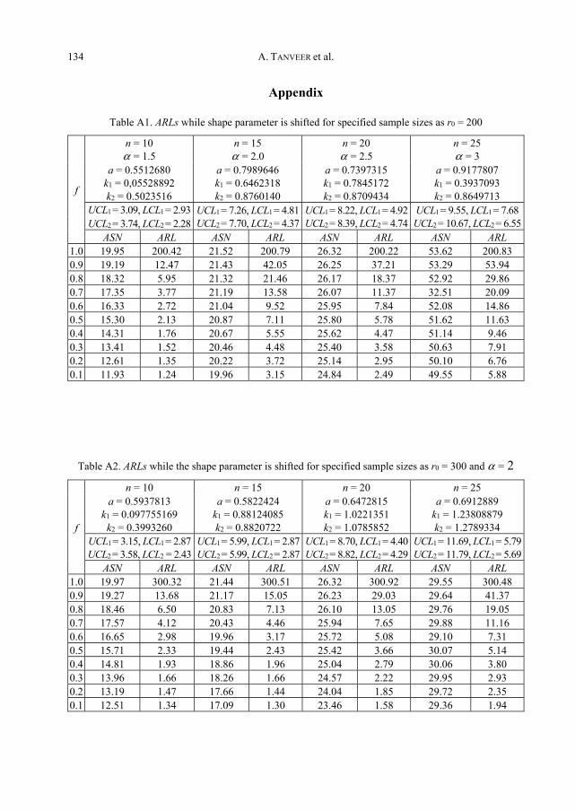
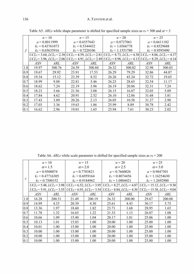
Results are simulated using the proposed control chart and algorithm and are pre-sented in tables. Tables A1–A5 present optimal parameters such as control coefficients k2 and k1 for fixed sample size (n). These parameters are calculated to get ARL value as close as the specified in-control ARL = 200, 300, and 370. Shape parameter α = 1.5, 2.0, 2.5, 3.0, shift constant f from 1.0 to 0.1, and sample sizes n = 10, 15, 20, 25 are chosen. It is found that ARL and ASN are decreasing if the shift constant is decreasing.

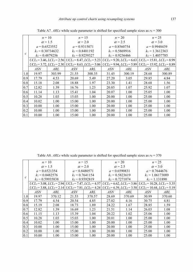
Tables A6–A8 present the optimal parameters for the shift in scale parameter, using shift c from 1.0 to 0.1.

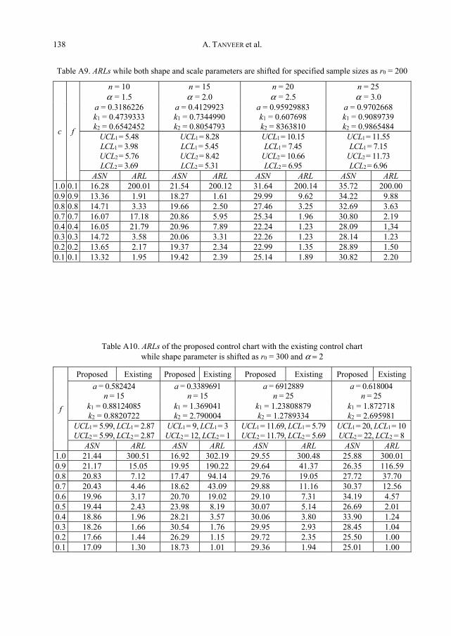
Table A9 gives the optimal parameters for the shift in both shape and scale param-eters for α = 1.5, 2.0, 2.5, and 3.0, using shift c and f from 1.0 to 0.1.

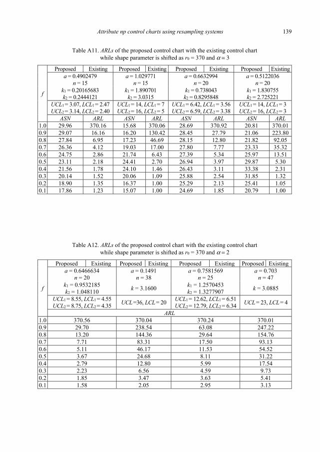
In this segment, the control chart performance in RGS is contrasted with the available control chart presented by Jeyadurga et al. [12] as based on EHLD. Tables A10 and A11 demonstrate the optimum parameters n, a, k1, k2, higher and lower control boundaries along with ARL and ASN values, using RGS scheme for the shape parameter α = 2 and 3 and specified r0 = 300 and 370. These tables show that the proposed chart identifies the change quicker than the existing one. For example, when r0 = 300, α = 2 and n = 25, the proposed control chart identifies the shift at 41th observation and ASN = 29.64. However, the shift is identified by the existing control chart at 116th observation.

The control chart performance in RGS is also contrasted with another available con-trol chart presented by Rao [6] as based on EHLD. Tables A12 and A13 demonstrate the optimum parameters, higher and lower control boundaries, ARL values using RGS scheme, and single sampling scheme for shape parameter α = 2 and r0 = 370, and for the scale parameter α = 2.5, 3, and r0 = 370. The proposed control chart identifies the change quicker than the existing one. For example, when r0 = 370, α = 2 and n = 25, the proposed chart identifies the shift at 63rd observation. However, the shift is identi-fied by the existing control chart at 247th observation. The shift in scale parameter is also shifted earlier, using the proposed control chart.


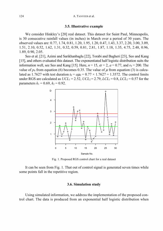
3.5. Illustrative example

We consider Hinkleyʼs [20] real dataset. This dataset for Saint Paul, Minneapolis, is 30 consecutive rainfall values (in inches) in March over a period of 30 years. The observed values are: 0.77, 1.74, 0.81, 1.20, 1.95, 1.20, 0.47, 1.43, 3.37, 2.20, 3.00, 3.09, 1.51, 2.10, 0.52, 1.62, 1.31, 0.32, 0.59, 0.81, 2.81, 1.87, 1.18, 1.35, 4.75, 2.48, 0.96, 1.89, 0.90, 2.05.

Seo et al. [21], Azimi and Sarikhanbaglu [22], Torabi and Bagheri [23], Seo and Kang [15], and others evaluated this dataset. The exponentiated half logistic distribution suits the information well, see Seo and Kang [15]. Here, n = 15, α = 2, a = 0.77, and r0 = 200. The value of p0 from equation (6) becomes 0.35. The value of μ from equation (3) is calcu-lated as 1.7627 with test duration t0 = aμ0 = 0.77 × 1.7627 = 1.3572. The control limits under RGS are calculated as UCL1 = 2.52, UCL2

= 2.79, LCL1 = 0.8, LCL2 = 0.57 for the

parameters k1 = 0.69, k2 = 0.92.

Fig. 1. Proposed RGS control chart for a real dataset

It can be seen from Fig. 1. That out of control signal is generated seven times while some points fall in the repetitive region.

3.6. Simulation study

Using simulated information, we address the implementation of the proposed con-trol chart. The data is produced from an exponential half logistic distribution when


α = 3 and σ = 1. Let n = 25, a = 0.76, and r0 = 370. The process is declared to be in-control when α = 3 and σ = 1. The value of p0 from equation (6) is calculated as 0.3082, μ = 2.16, the test duration is therefore calculated as t0 = aμ0 = 0.76 × 2.16

= 1.64. The value of d = Σdi/l = 6.6 and l = 20. We find out the control limits coef-ficients k1 = 1.06173089 and k2 = 1.131890 and control limits are UCL1 = 8.94, UCL2 = 9.09, LCL1 = 4.25, LCL2 = 4.10, the amount of failures per subgroup is reported before the specified time.

Table 1. The simulated data

Subgroup 1 2 3 4 5 6 7 8 9 10 D 7 8 6 7 8 6 8 3 5 7

Subgroup 11 12 13 14 15 16 17 18 19 20 D 8 6 7 6 8 8 5 6 5 8

Fig. 2. The proposed RGS control chart for simulated data.

We can see from Fig. 2 that if the number of fail items in the subgroup is 5, 6, 7, or 8, the process is said to be in-control. The sampling will be repeated if the subgroup in-cludes 9 failed items. If the number of failures is less than or equal to 4, the process is said to be out of control.

4. Design of the proposed control chart under MDS

Under the MDS scheme, the decision about the in-control or the out of control pro-cess is made, considering the results of the previous samples. If we select a sample from


the online process and post it on the control chart, then it may fall in any of three mutu-ally exclusive states, i.e., in-control state, out of control state, or in the state in which the decision depends on the previous samples. Following are the steps of np control chart based on the MDS scheme.

Step 1. Choose from the production process a random sample of size n. Count failed items D for a specified time t = aμ0, where μ0 is the target mean when the process is in-control and a is constant.

Step 2. If LCL2 ≤ D ≤ UCL2, declare the process as in-control. If D > UCL1 or D < LCL1, declare the process as out of control. For all the other cases, repeat the process until ith sample and declare the process as in-control if LCL2 ≤ D ≤ UCL2 for all i samples.

The method is stated to be controlled when t = aμ0, μ = μ0. We express the scale parameter σ in terms of μ using equation (3b), and then equation (1) can be rewritten as

01 e1 e

a

apαη

η

−

−

−= + (16)

4.1. Shift in scale and shape parameters

We are designing a chart for monitoring mean shift. Assume that the process mean is shifted from μ = μ0 and μ1 = cμ0, then equation (1) becomes

/

1 /1 e1 e

a c

a cpαη

η

−

−

−= + (17)

If the shape parameter is shifted from α0 to α1 = fα0 (or the shape parameter is α = α1), then equation (1) becomes

0 01

01

1/

2 1 1/1 e 1 0.5where ln1 e 1 0.5

f fa

fapα αη

αη η−

−

− += = + − (18)

4.2. Shift in both shape and scale parameters

Suppose that the shape and scale of both parameters are shifted to α1 = fα0 and σ1 = cσ0

(now the shape parameter is α1 and the scale parameter is σ1). The likelihood that an item is failed p3 is specified as


0 01

01

1//

3 1 1//1 e 1 0.5where ln1 e 1 0.5

f fa c

fa cpα αη

αη η−

−

− += = + − (19)

The probability that the process is stated in-control if the process is in-control is

( ) ( )(

( ) ) ( )( )2 2 1 2

2 1 2 2

in

i

P P LCL D UCL P LCL D LCL

P UCL D UCL P LCL D UCL

= ≤ ≤ + ≤ ≤

+ ≤ ≤ × ≤ ≤

( ) ( ) ( ) ( )(

( ) ( )) ( ) ( )( )

0

2 2 1 20

12 2 2

in

i

P P d LCL P d UCL P d LCL P d LCLp

P d UCL P d P d LCL P d UCLUCL

= ≥ + ≤ + ≥ + ≤

+ ≥ + ≤ × ≥ + ≤

[ ]( ) ( )

[ ]

( ) ( )[ ]

[ ]

( ) ( )[ ]

[ ]

( )

2

2

2

1

1

2

0

0 0 0 01 00

0 0 0 01 0

0 0 0 01 0

0 0

1 1

1 1

1 1

1

UCLnn d n dd din

d LCL d

LCLnn d n dd d

d LCL d

UCLnn d n dd d

d UCL d

nd

n nP p p p pd dp

n np p p p

d d

n np p p p

d d

np p

d

− −

= + =

− −

= + =

− −

= + =

−

= − + −

+ − + −

+ − + −

× −

( )[ ]

[ ]

2

2

0 01 0

1iUCLn

d n dd

d LCL d

np p

d−

= + =

+ −

[ ]

[ ]( )

[ ]

[ ]( )

[ ]

[ ]( )

[ ]

[ ]( )

2

2

2 1

1 2

2

2

0

0 010

0 0 0 01 1

0 01

1

1 1

1

UCLn ddin

d LCL

LCL UCLn d n dd d

d dLCL UCL

iUCL

n dd

d LCL

nP p pdp

n np p p p

d d

np p

d

−

= +

− −

= + = +

−

= +

= −

+ − + −

× −

(20)

Likewise, the probability that the process will be stated in-control when the process is shifted to μ1 is specified as


[ ]

[ ]( )

[ ]

[ ]( )

[ ]

[ ]( )

[ ]

[ ]( )

2

2

2 1

1 2

2

2

1

1 111

1 1 1 11 1

1 11

1

1 1

1

UCLn ddin

d LCL

LCL UCLn d n dd d

d dLCL UCL

iUCL

n dd

d LCL

nP p pdp

n np p p p

d d

np p

d

−

= +

− −

= + = +

−

= +

= −

+ − + −

× −

(21)

Likewise, the probability when the shape parameter is shifted is specified as

[ ]

[ ]( )

[ ]

[ ]( )( )

[ ]

[ ]( )

[ ]

[ ]( )

2

2

2 1

1 2

2

2

2 212

2 2 2 21 1

2 212

1

1 1

1

UCLn ddin

d LCL

LCL UCLn d n dd d

d dLCL UCL

iUCL

n dd

d LCL

nP p pdp

n np p p p

d d

np p

d

−

= +

− −

= + = +

−

= +

= −

+ − + −

× −

(22)

Likewise, the probability when both shape and scale parameters are shifted is

[ ]

[ ]( )

[ ]

[ ]( )

[ ]

[ ]( )

[ ]

[ ]( )

2

2

2 1

1 2

2

2

3

3 313

3 3 3 31 1

3 31

1

1 1

1

UCLn ddin

d LCL

LCL UCLn d n dd d

d dLCL UCL

iUCL

n dd

d LCL

nP p pdp

n np p p p

d d

np p

d

−

= +

− −

= + = +

−

= +

= −

+ − + −

× −

(23)

The average run length (ARL) is used to evaluate the efficiency of a control chart. The in-control ARL and out of control ARL are given in equations (24), (25), (26), and (27), respectively.

0 01

1 in

ARLP

=−

(24)

1 11

1 in

ARLP

=−

(25)


2 21

1 in

ARLP

=−

(26)

3 31

1 in

ARLP

=−

(27)

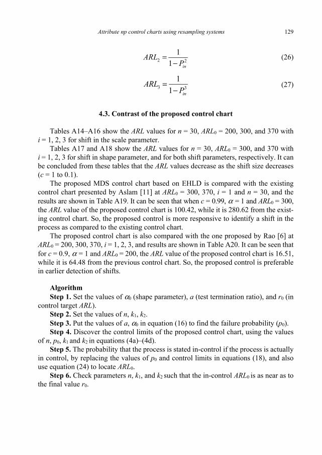
4.3. Contrast of the proposed control chart

Tables A14–A16 show the ARL values for n = 30, ARL0 = 200, 300, and 370 with i = 1, 2, 3 for shift in the scale parameter.

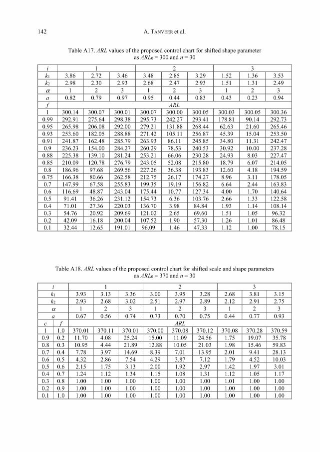
Tables A17 and A18 show the ARL values for n = 30, ARL0 = 300, and 370 with i = 1, 2, 3 for shift in shape parameter, and for both shift parameters, respectively. It can be concluded from these tables that the ARL values decrease as the shift size decreases (c = 1 to 0.1).

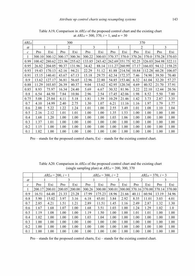
The proposed MDS control chart based on EHLD is compared with the existing control chart presented by Aslam [11] at ARL0 = 300, 370, i = 1 and n = 30, and the results are shown in Table A19. It can be seen that when c = 0.99, α = 1 and ARL0 = 300, the ARL value of the proposed control chart is 100.42, while it is 280.62 from the exist-ing control chart. So, the proposed control is more responsive to identify a shift in the process as compared to the existing control chart.

The proposed control chart is also compared with the one proposed by Rao [6] at ARL0 = 200, 300, 370, i = 1, 2, 3, and results are shown in Table A20. It can be seen that for c = 0.9, α = 1 and ARL0 = 200, the ARL value of the proposed control chart is 16.51, while it is 64.48 from the previous control chart. So, the proposed control is preferable in earlier detection of shifts.

Algorithm Step 1. Set the values of α0 (shape parameter), a (test termination ratio), and r0 (in

control target ARL). Step 2. Set the values of n, k1, k2. Step 3. Put the values of a, α0 in equation (16) to find the failure probability (p0). Step 4. Discover the control limits of the proposed control chart, using the values

of n, p0, k1 and k2 in equations (4a)–(4d). Step 5. The probability that the process is stated in-control if the process is actually

in control, by replacing the values of p0 and control limits in equations (18), and also use equation (24) to locate ARL0.

Step 6. Check parameters n, k1, and k2 such that the in-control ARL0 is as near as to the final value r0.


Step 7. Continue Steps 4–6 for various combinations of n, k1, and k2 until you get an ARL0 as near as to r0.

Step 8. Replace the values n, k1, and k2 in equations (17)–(23), (25)–(27) for dis-covering the out of control ARL1 for various shift values.

4.4. Illustrative example

We consider Hinkleyʼs [20] real dataset. This dataset for Saint Paul, Minneapolis, is 30 consecutive rainfall values (in inches) in March over a period of 30 years. The observed values are: 0.77, 1.74, 0.81, 1.20, 1.95, 1.20, 0.47, 1.43, 3.37, 2.20, 3.00, 3.09, 1.51, 2.10, 0.52, 1.62, 1.31, 0.32, 0.59, 0.81, 2.81, 1.87, 1.18, 1.35, 4.75, 2.48, 0.96, 1.89, 0.90, 2.05.

Seo et al. [21], Azimi and Sarikhanbaglu [22], Torabi and Bagheri [23], Seo and Kang [15], and others evaluated this dataset. The exponentiated half logistic distribution suits the information well [15]. Here, n = 30, α = 2, i = 1, a = 0.32, and r0 = 370. The value of p0 from equation (16) becomes 0.075. The value of μ from equation (3) is cal-culated as 1.7627 with test duration t0 = aμ0 = 0.32 × 1.7627 = 0.564. The control limits under MDS calculated are UCL1 = 3.15, UCL2 = 2.64 LCL1 = 0.21, LCL2 = 0.72 for the parameters k1 = 1.17, k2 = 0.76.

Fig. 3. The proposed MDS control chart for a real dataset

It can be seen from Fig. 3 that out of control signal is generated twice, while some points fall in the repetitive region.


4.5. Simulation study

In this study, using simulated information, we address the implementation of the pro-posed control chart. The data is produced from an exponential half logistic distribution when α = 3 and σ = 1. Let n = 30, a = 0.88, and r0 = 370. The process is declared to be in-control when α = 3 and σ = 1. The value of p0 from equation (16) is calculated as 0.4092, μ = 2.16, the test duration is therefore calculated as t0 = aμ0 = 0.88 × 2.16 = 1.90. The value of

/id d l= = 12.275 and l = 40. We find out the control limits coefficients k1 = 2.735302, and k2 = 2.324929, and control limits are UCL1 = 19.64, UCL2 = 18.54, LCL1 = 4.91, LCL2 = 6.01, the number of failures per subgroup is reported before the specified time. If the number of fail items in the subgroup is 7–18, the process is said to be in-control. The sampling will be repeated if the subgroup includes 5, 6 or 19 failed items. If the number of failures is less than or equal to 4, the process is stated to be out of control (Fig. 4). By comparing Figs. 4 and 5, we can conclude that the proposed control chart has the ability to detect a small shift in the process earlier than the existing control chart.

Table 2. The simulated data

Subgroup 1 2 3 4 5 6 7 8 9 10 11 12 13 14 15 16 17 18 19 20 D 11 11 15 11 13 13 9 11 16 14 14 13 17 19 16 8 16 15 11 11

Subgroup 21 22 23 24 25 26 27 28 29 30 31 32 33 34 35 36 37 38 39 40 D 13 12 11 13 12 10 6 13 10 12 11 15 11 10 15 7 11 14 12 11

Fig. 4. The proposed MDS control chart for simulated data

D


Fig. 5. Aslamʼs [11] chart for simulated data

5. Conclusion

We propose an attribute np control chart under RGS and MDS based on time trun-cated life tests for EHLD. The performance of the proposed control chart is evaluated in terms of ARL. The optimal parameters used for constructing the chart are determined such that the in-control ARL is as close as to the specified value of ARL. The perfor-mance of the proposed chart is compared with the performance of the chart developed by Jeyadurga et al. [12]. The control chart performance in RGS is also contrasted with the control chart presented by Rao [6], based on EHLD. Results are presented in the form of tables, using different scales and shape parameters. These tables show that the proposed chart identifies the change quicker than the existing chart. The efficiency of the proposed MDS control chart is compared to the control chart results by Aslam [11]. The results indicate that the proposed control chart is more responsive than the existing one to recognize a shift in the process. The efficiency of the proposed MDS control chart is also compared to Raoʼs [6] results and concluded in the form of tables using different ARL0 values. It is concluded that the proposed control is more responsive to identify a shift in the process as compared to the existing control chart. For future work, the proposed control chart might be applied to other distributions.

Acknowledgements The authors are deeply thankful to the Editor and the Reviewers for their valuable suggestions that had

led to improve the quality of this manuscript.

D


References

[1] SHERMAN R.E., Design and evaluation of a RGS plan, Technometrics, 1965, 7, 11–21. [2] BALAMURALI S., JUN C.-H., Repetitive group sampling procedure for variables inspection, J. Appl.

Stat., 2006, 33, 327–338. [3] AHMAD L., ASLAM M., JUN C.-H., Designing of X-bar control charts based on process capability index

using repetitive sampling, Trans. Inst. Measure. Control, 2014, 36, 367–374. [4] ASLAM M., AZAM M., JUN C.-H., New attributes and variables control charts under repetitive sam-

pling, Ind. Eng. Manage. Syst., 2014, 13, 101–106. [5] ASLAM M., KHAN N., AZAM M., JUN C.-H., Designing of a new monitoring t-chart using repetitive

sampling, Inf. Sci., 2014, 269, 210–216. [6] RAO G., A control chart for time truncated life tests using exponentiated half logistic distribution,

Appl. Math. Inf. Sci., 2018, 12, 125–131. [7] WORTHAM A., BAKER R., Multiple deferred state sampling inspection, Int. J. Prod. Res., 1976, 14, 719–731. [8] ASLAM M., YEN C.-H., CHANG C.-H., JUN C.-H., Multiple dependent state variable sampling plans

with process loss consideration, Int. J. Adv. Manuf. Techn., 2014, 71, 1337–1343. [9] ASLAM M., KHAN N., JUN C.-H., A multiple dependent state control chart based on double control

limits, Res. J. Appl. Sci. Eng. Techn., 2014, 7, 4490–4493. [10] RAO G.S., NAIDU C., Acceptance sampling plans for percentiles based on the exponentiated half lo-

gistic distribution, Appl. Appl. Math., 2014, 9, 39–53. [11] ASLAM M., Time truncated attribute control chart for the Weibull distribution using MDS, Comm.

Stat.-Sim. Comp., 2019, 48, 1219–1228. [12] JEYADURGA P., BALAMURALI S., ASLAM M., Design of an attribute np control chart for process moni-

toring based on repetitive group sampling under truncated life tests, Comm. Stat.-Theory Meth., 2018, 47, 5934–5955.

[13] MUDHOLKAR G.S., SRIVASTAVA D.K., Exponentiated Weibull family for analyzing bathtub failure-rate data, IEEE Trans. Rel., 1993, 42, 299–302.

[14] CORDEIRO G.M., ALIZADEH M., ORTEGA E.M., The exponentiated half-logistic family of distributions: Properties and applications, J. Prob. Stat., 2014, 2014.

[15] SEO J.-I., KANG S.-B., Notes on the exponentiated half logistic distribution, Appl. Math. Model., 2015, 39, 6491–6500.

[16] ELGARHY M., HAQ M., OZEL G., A new exponentiated extended family of distributions with applica-tions, Gazi University J. Sci., 2017, 30, 101–115.

[17] USMAN R.M., HAQ M., TALIB J., Kumaraswamy half-logistic distribution: properties and applications, J. Stat. Appl. Prob., 2017, 6, 597–609.

[18] ANWAR M., BIBI A., The half-logistic generalized Weibull distribution, J. Prob. Stat., 2018, 2018. [19] MONTGOMERY D.C., Introduction to statistical quality control, Wiley, 2007. [20] HINKLEY D., On quick choice of power transformation, J. Royal Stat. Soc., Series C, 1977, 26, 67–69. [21] SEO J.-I., LEE H.-J., KAN S.-B., Estimation for generalized half logistic distribution based on records,

J. Korean Data Inf. Sci. Soc., 2012, 23, 1249–1257. [22] AZIMI R., SARIKHANBAGLU F.A., Bayes and empirical bayes estimators based on generalized half lo-

gistic records data, Journal of Statistics Appl. Prob., 2014, 3, 145?. [23] TORABI H., BAGHERI F., Estimation of parameters for an extended generalized half logistic distribution

based on complete and censored data, J. Iranian Stat. Soc., 2010, 9, 171–195.


Appendix

Table A1. ARLs while shape parameter is shifted for specified sample sizes as r0 = 200

f

n = 10 α = 1.5

n = 15 α = 2.0

n = 20 α = 2.5

n = 25 α = 3

a = 0.5512680 k1 = 0,05528892 k2 = 0.5023516

a = 0.7989646 k1 = 0.6462318 k2 = 0.8760140

a = 0.7397315 k1 = 0.7845172 k2 = 0.8709434

a = 0.9177807 k1 = 0.3937093 k2 = 0.8649713

UCL1 = 3.09, LCL1 = 2.93 UCL1 = 7.26, LCL1 = 4.81 UCL2 = 7.70, LCL2 = 4.37

UCL1 = 8.22, LCL1 = 4.92 UCL2 = 8.39, LCL2 = 4.74

UCL1 = 9.55, LCL1 = 7.68 UCL2 = 10.67, LCL2 = 6.55 UCL2 = 3.74, LCL2 = 2.28

ASN ARL ASN ARL ASN ARL ASN ARL 1.0 19.95 200.42 21.52 200.79 26.32 200.22 53.62 200.83 0.9 19.19 12.47 21.43 42.05 26.25 37.21 53.29 53.94 0.8 18.32 5.95 21.32 21.46 26.17 18.37 52.92 29.86 0.7 17.35 3.77 21.19 13.58 26.07 11.37 32.51 20.09 0.6 16.33 2.72 21.04 9.52 25.95 7.84 52.08 14.86 0.5 15.30 2.13 20.87 7.11 25.80 5.78 51.62 11.63 0.4 14.31 1.76 20.67 5.55 25.62 4.47 51.14 9.46 0.3 13.41 1.52 20.46 4.48 25.40 3.58 50.63 7.91 0.2 12.61 1.35 20.22 3.72 25.14 2.95 50.10 6.76 0.1 11.93 1.24 19.96 3.15 24.84 2.49 49.55 5.88

Table A2. ARLs while the shape parameter is shifted for specified sample sizes as r0 = 300 and α = 2

f

n = 10 n = 15 n = 20 n = 25 a = 0.5937813

k1 = 0.097755169 k2 = 0.3993260

a = 0.5822424 k1 = 0.88124085 k2 = 0.8820722

a = 0.6472815 k1 = 1.0221351 k2 = 1.0785852

a = 0.6912889 k1 = 1.23808879 k2 = 1.2789334

UCL1 = 3.15, LCL1 = 2.87 UCL2 = 3.58, LCL2 = 2.43

UCL1 = 5.99, LCL1 = 2.87 UCL2 = 5.99, LCL2 = 2.87

UCL1 = 8.70, LCL1 = 4.40 UCL2 = 8.82, LCL2 = 4.29

UCL1 = 11.69, LCL1 = 5.79 UCL2 = 11.79, LCL2 = 5.69



Table A3. ARLs while shape parameter is shifted for specified sample sizes as r0 = 370 and α = 2

f

n = 10 n = 15 n = 20 n = 25 a = 0.9424639

k1 = 0.52002428 k2 = 0.559912

a = 0.7967768 k1 = 0.71566975 k2 = 0.9685180

a = 0.6466634 k1 = 0.9532185 k2 = 1.048110

a = 0.7581569 k1 = 1.2570453 k2 = 1.3277907

UCL1 = 5.54, LCL1 = 3.90 UCL2 = 5.61, LCL2 = 3.84

UCL1 = 7.38, LCL1 = 4.66 UCL2 = 7.86, LCL2 = 4.18

UCL1 = 8.55, LCL1 = 4.55 UCL2 = 8.75, LCL2 = 4.35

UCL1 = 12.62, LCL1 = 6.51 UCL2 = 12.79, LCL2 = 6.34



f

n = 10 n = 15 n = 20 n = 25 a = 0.8008269

k1 = 0.18693262 k2 = 0.5685758

a = 0.4902479 k1 = 0.20165683 k2 = 0.2444121

a = 0.6632994 k1 = 0.738043 k2 = 0.8295848

a = 0.7582928 k1 = 1.2195140 k2 = 1.2490227

UCL1 = 3.28, LCL1 = 2.74 UCL2 = 3.83, LCL2 = 2.18

UCL1 = 3.07, LCL1 = 2.47 UCL2 = 3.14, LCL2 = 2.40

UCL1 = 6.42, LCL1 = 3.56 UCL2 = 6.59, LCL2 = 3.38

UCL1 = 9.88, LCL1 = 4.37 UCL2 = 9.94, LCL2 = 4.31




f

n = 10 n = 15 n = 20 n = 25 a = 0.8011999

k1 = 0.43761073 k2 = 0.65635916

a = 0.6557643 k1 = 0.5344432 k2 = 0.7220106

a = 0.8727061 k1 = 1.0366778 k2 = 1.1551780

a = 0.6611102 k1 = 0.8529688 k2 = 0.9595490

UCL1 = 3.64, LCL1 = 2.38 UCL2 = 3.96, LCL2 = 2.06

UCL1 = 4.59, LCL1 = 2.81 UCL2 = 4.91, LCL2 = 2.49

UCL1 = 8.73, LCL1 = 4.38 UCL2 = 8.98, LCL2 = 4.13

UCL1 = 8.06, LCL1 = 4.37 UCL2 = 8.29, LCL2 = 4.14


Table A6. ARLs while scale parameter is shifted for specified sample sizes as r0 = 200

c

n = 10 α = 1.5

n = 15 α = 2.0

n = 20 α = 2.5

n = 25 α = 3.0

a = 0.9500074 k1 = 0.47716305 k2 = 0.7500152

a = 0.7703821 k1 = 0.6959164 k2 = 0.9184962

a = 0.7660026 k1 = 0.8074456 k2 = 1.0804421

a = 0.9847301 k1 = 1.16254630 k2 = 1.2692900

UCL1 = 5.48, LCL1 = 3.98 UCL2 = 5.91, LCL2 = 3.55

UCL1 = 6.52, LCL1 = 3.95 UCL2 = 6.93, LCL2 = 3.54

UCL1 = 8.27, LCL1 = 4.87 UCL2 = 8.84, LCL2 = 4.30

UCL1 = 15.12, LCL1 = 9.30 UCL2 = 15.38, LCL2 = 9.04




c

n = 10 α = 1.5

n = 15 α = 2.0

n = 20 α = 2.5

n = 25 α = 3.0

a = 0.6523552 k1 = 0.30734632 k2 = 0.4879256

a = 0.9315071 k1 = 0.8401192 k2 = 0.9259327

a = 0.8560754 k1 = 0.5869916 k2 = 0.9236466

a = 0.9948439 k1 = 1.3612363 k2 = 1.4057785

UCL1 = 3.46, LCL1 = 2.56 UCL2 = 3.72, LCL2 = 2.30

UCL1 = 8.47, LCL1 = 5.23 UCL2 = 8.63, LCL2 = 5.06

UCL1 = 9.20, LCL1 = 6.63 UCL2 = 9.94, LCL2 = 5.89

UCL1 = 15.81, LCL1 = 8.99 UCL2 = 15.92, LCL2 = 8.89



c

n = 10 α = 1.5

n = 15 α = 2.0

n = 20 α = 2.5

n = 25 α = 3.0

a = 0.6521354 k1 = 0.0482576 k2 = 0.59935838

a = 0.8480571 k1 = 0.7641154 k2 = 0.9392819

a = 0.6590831 k1 = 0.5823619 k2 = 0.7271074

a = 0.7644676 k1 = 1.06173089

k2 = 1.131890 UCL1 = 3.08, LCL1 = 2.94 UCL2 = 3.88, LCL2 = 2.14

UCL1 = 7.47, LCL1 = 4.57 UCL2 = 7.81, LCL2 = 4.24

UCL1 = 6.62, LCL1 = 3.86 UCL2 = 6.39, LCL2 = 3.58

UCL1 = 10.28, LCL1 = 5.35 UCL2 = 10.44, LCL2 = 5.19



Table A9. ARLs while both shape and scale parameters are shifted for specified sample sizes as r0 = 200

c f

n = 10 α = 1.5

n = 15 α = 2.0

n = 20 α = 2.5

n = 25 α = 3.0

a = 0.3186226 k1 = 0.4739333 k2 = 0.6542452

a = 0.4129923 k1 = 0.7344990 k2 = 0.8054793

a = 0.95929883 k1 = 0.607698 k2 = 8363810

a = 0.9702668 k1 = 0.9089739 k2 = 0.9865484

UCL1 = 5.48 LCL1 = 3.98 UCL2 = 5.76 LCL2 = 3.69

UCL1 = 8.28 LCL1 = 5.45 UCL2 = 8.42 LCL2 = 5.31

UCL1 = 10.15 LCL1 = 7.45

UCL2 = 10.66 LCL2 = 6.95

UCL1 = 11.55 LCL1 = 7.15

UCL2 = 11.73 LCL2 = 6.96

ASN ARL ASN ARL ASN ARL ASN ARL 1.0 0.1 16.28 200.01 21.54 200.12 31.64 200.14 35.72 200.00 0.9 0.9 13.36 1.91 18.27 1.61 29.99 9.62 34.22 9.88 0.8 0.8 14.71 3.33 19.66 2.50 27.46 3.25 32.69 3.63 0.7 0.7 16.07 17.18 20.86 5.95 25.34 1.96 30.80 2.19 0.4 0.4 16.05 21.79 20.96 7.89 22.24 1.23 28.09 1,34 0.3 0.3 14.72 3.58 20.06 3.31 22.26 1.23 28.14 1.23 0.2 0.2 13.65 2.17 19.37 2.34 22.99 1.35 28.89 1.50 0.1 0.1 13.32 1.95 19.42 2.39 25.14 1.89 30.82 2.20

Table A10. ARLs of the proposed control chart with the existing control chart while shape parameter is shifted as r0 = 300 and α = 2

f

Proposed Existing Proposed Existing Proposed Existing Proposed Existing a = 0.582424

n = 15 a = 0.3389691

n = 15 a = 6912889

n = 25 a = 0.618004

n = 25 k1 = 0.88124085 k2 = 0.8820722

k1 = 1.369041 k2 = 2.790004

k1 = 1.23808879 k2 = 1.2789334

k1 = 1.872718 k2 = 2.695981

UCL1 = 5.99, LCL1 = 2.87 UCL2 = 5.99, LCL2 = 2.87

UCL1 = 9, LCL1 = 3 UCL2 = 12, LCL2 = 1

UCL1 = 11.69, LCL1 = 5.79 UCL2 = 11.79, LCL2 = 5.69

UCL1 = 20, LCL1 = 10 UCL2 = 22, LCL2 = 8




f


n = 15 a = 1.029771

n = 15 a = 0.6632994

n = 20 a = 0.5122036

n = 20 k1 = 0.20165683 k2 = 0.2444121

k1 = 1.890701 k2 = 3.0315

k1 = 0.738043 k2 = 0.8295848

k1 = 1.830755 k2 = 2.725221

UCL1 = 3.07, LCL1 = 2.47 UCL2 = 3.14, LCL2 = 2.40

UCL1 = 14, LCL1 = 7 UCL2 = 16, LCL2 = 5

UCL1 = 6.42, LCL1 = 3.56 UCL2 = 6.59, LCL2 = 3.38

UCL1 = 14, LCL1 = 3 UCL2 = 16, LCL2 = 3



f


n = 20 a = 0.1491

n = 38 a = 0.7581569

n = 25 a = 0.703

n = 47 k1 = 0.9532185 k2 = 1.048110 k = 3.1600 k1 = 1.2570453

k2 = 1.3277907 k = 3.0885

UCL1 = 8.55, LCL1 = 4.55 UCL2 = 8.75, LCL2 = 4.35 UCL =36, LCL = 20 UCL1 = 12.62, LCL1 = 6.51

UCL2 = 12.79, LCL2 = 6.34 UCL = 23, LCL = 4

ARL 1.0 370.56 370.04 370.24 370.01 0.9 29.70 238.54 63.08 247.22 0.8 13.20 144.36 29.64 154.76 0.7 7.71 83.31 17.50 93.13 0.6 5.11 46.17 11.53 54.52 0.5 3.67 24.68 8.11 31.22 0.4 2.79 12.80 5.99 17.54 0.3 2.23 6.56 4.59 9.73 0.2 1.85 3.47 3.63 5.41 0.1 1.58 2.05 2.95 3.13


Table A13. ARLs of the proposed control chart with the existing control chart while scale parameter is shifted as r0 = 370

c


n = 20 a = 0.841

n = 23 a = 0.7644676

n = 23 a = 0.957

n = 46 α = 2.5 α = 2.5 α = 3 α = 3

k1 = 0.9532185 k2 = 1.048110 k = 3.1600 k1 = 1.2570453

k2 = 1.3277907 k = 3.0885

UCL1 = 6.62, LCL1 = 3.86 UCL2 = 6.39, LCL2 = 3.58 UCL = 15, LCL = 1 UCL1 = 10.28, LCL1 = 5.35

UCL2 = 10.44, LCL2 = 5.19 UCL = 31, LCL = 11

ARL 1.0 370.69 37.02 370.60 370.00 0.9 4.16 59.92 4.81 34.96 0.8 1.67 11.16 1.59 4.01 0.7 1.14 2.99 1.08 1.30 0.6 1.02 1.34 1.00 1.01 0.5 1.00 1.03 1.00 1.00 0.4 1.00 1.00 1.00 1.00 0.3 1.00 1.00 1.00 1.00 0.2 1.00 1.00 1.00 1.00 0.1 1.00 1.00 1.00 1.00

Table A14. ARL values of the proposed control chart for the shifted scale parameter as ARL0 = 200 and n = 30

i 1 2 3 k1 1.21 3.83 3.91 3.13 1.72 2.87 3.24 3.44 2.81 k2 1.15 3.49 2.94 2.91 1.55 2.42 2.73 2.75 2.35 α 1 2 3 1 2 3 1 2 3 a 0.35 0.27 0.72 0.29 0.73 0.96 0.21 0.96 0.87 c ARL 1 200.17 200.04 200.05 200.01 200.03 200.07 200.01 200.05 200.02

0.99 114.62 182.13 152.94 185.17 96.87 124.76 187.19 151.90 128.95 0.95 36.50 124.64 59.90 135.48 23.40 40.02 142.99 63.27 42.76 0.93 25.48 102.85 39.09 115.61 14.85 26.13 124.68 43.35 28.01 0.91 18.88 84.75 5.99 98.50 10.11 17.71 108.52 30.33 18.99 0.9 16.51 76.89 21.33 90.87 8.50 14.73 101.18 25.54 15.79

0.88 12.92 63.22 14.58 77.24 6.20 10.37 87.84 18.33 11.09 0.85 9.34 47.03 8.55 60.37 4.11 6.40 70.83 11.52 6.81 0.8 5.90 28.59 3.97 39.75 2.39 3.23 49.06 5.86 3.39

0.75 3.99 17.33 2.21 25.98 1.63 1.92 33.63 3.39 1.98 0.7 2.85 10.54 1.51 16.88 1.27 1.35 22.83 2.19 1.37 0.6 1.67 4.06 1.07 7.10 1.03 1.02 10.26 1.20 1.03 0.5 1.19 1.82 1.00 3.10 1.00 1.00 4.57 1.01 1.00 0.4 1.02 1.12 1.00 1.56 1.00 1.00 2.14 1.00 1.00 0.3 1.00 1.00 1.00 1.06 1.00 1.00 1.22 1.00 1.00 0.2 1.00 1.00 1.00 1.00 1.00 1.00 1.00 1.00 1.00 0.1 1.00 1.00 1.00 1.00 1.00 1.00 1.00 1.00 1.00


Table A15. ARL values of the proposed control chart for shifted scale parameter as ARL0 = 300 and n = 30

i 1 2 3 k1 3.38 3.09 2.74 1.19 2.73 2.78 3.38 2.69 3.60 k2 0.12 2.82 2.21 1.18 2.45 2.39 2.95 2.28 3.09 α 1 2 3 1 2 3 1 2 3 a 0.02 0.77 0.88 0.39 0.79 0.82 0.24 0.94 0.52 c ARL 1 300.10 300.17 300.22 300.26 300.10 300.01 300.07 300.02 300.50

0.99 100.42 221.96 133.85 146.68 192.57 175.88 278.81 177.36 250.52 0.95 26.82 90.37 34.42 41.19 67.14 53.03 206.88 56.84 121.92 0.93 19.43 62.16 22.29 28.26 45.69 34.22 177.72 38.20 85.54 0.91 15.15 43.67 15.18 20.69 32.19 22.93 152.400 26.70 60.31 0.9 13.62 36.81 12.69 17.99 27.24 18.96 141.03 22.54 50.75

0.88 11.29 26.39 9.04 13.96 19.76 13.18 120.60 16.29 36.10 0.85 8.93 16.38 5.69 9.97 12.52 7.96 95.05 10.32 21.97 0.8 6.54 7.84 2.96 6.18 6.26 3.84 63.34 5.21 10.08

0.75 5.08 4.11 1.81 4.11 3.43 2.16 41.74 2.92 5.00 0.7 4.10 2.40 1.30 2.89 2.10 1.45 27.23 1.86 2.76 0.6 2.88 1.22 1.01 1.68 1.17 1.03 11.32 1.12 1.27 0.5 2.16 1.01 1.00 1.19 1.01 1.00 4.69 1.00 1.01 0.4 1.68 1.00 1.00 1.03 1.00 1.00 2.09 1.00 1.00 0.3 1.37 1.00 1.00 1.00 1.00 1.00 1.18 1.00 1.00 0.2 1.15 1.00 1.00 1.00 1.00 1.00 1.00 1.00 1.00 0.1 1.02 1.00 1.00 1.00 1.00 1.00 1.00 1.00 1.00

Table A16. ARL values of the proposed control chart for shifted scale parameter as ARL0 = 370 and n = 30

i 1 2 3 k1 2.95 1.48 3.83 1.56 3.95 3.78 2.57 3.26 2.73 k2 2.43 1.32 2.86 1.51 3.02 3.49 2.10 2.61 2.32 α 1 2 3 1 2 3 1 2 3 a 0.69 0.84 0.71 0.92 0.87 0.39 0.51 0.77 0.88 c ARL 1 370.37 370.26 370.28 370.03 370.13 370.05 370.01 370.16 370.14

0.99 262.69 92.25 264.98 208.03 278.90 318.39 192.94 261.80 148.44 0.95 111.27 17.17 94.12 55.05 110.81 174.32 61.81 100.37 36.14 0.93 81.88 10.84 60.28 35.11 73.65 129.01 44.44 68.35 23.28 0.91 62.34 7.46 39.50 23.89 49.79 95.54 33.84 47.71 15.81 0.9 54.85 6.32 32.20 20.06 41.15 82.25 29.94 40.11 13.19

0.88 42.95 4.69 21.70 14.52 28.39 61.03 23.90 28.63 9.38 0.85 30.32 3.22 12.44 9.42 16.72 39.17 17.61 17.64 5.88 0.8 17.45 1.98 5.50 5.09 7.54 19.02 11.13 8.35 3.03

0.75 10.29 1.42 2.87 3.09 3.91 9.56 7.28 4.32 1.83 0.7 6.21 1.16 1.79 2.07 2.38 5.06 4.87 2.49 1.32 0.6 2.55 1.01 1.10 1.25 1.31 1.83 2.37 1.24 1.02 0.5 1.35 1.00 1.00 1.03 1.02 1.10 1.38 1.01 1.00 0.4 1.03 1.00 1.00 1.00 1.00 1.00 1.05 1.00 1.00 0.3 1.00 1.00 1.00 1.00 1.00 1.00 1.00 1.00 1.00 0.2 1.00 1.00 1.00 1.00 1.00 1.00 1.00 1.00 1.00 0.1 1.00 1.00 1.00 1.00 1.00 1.00 1.00 1.00 1.00


Table A17. ARL values of the proposed control chart for shifted shape parameter as ARL0 = 300 and n = 30

i 1 2 3 k1 3.86 2.72 3.46 3.48 2.85 3.29 1.52 1.36 3.53 k2 2.98 2.30 2.93 2.68 2.47 2.93 1.51 1.31 2.49 α 1 2 3 1 2 3 1 2 3 a 0.82 0.79 0.97 0.95 0.44 0.83 0.43 0.23 0.94 f ARL 1 300.14 300.07 300.01 300.07 300.00 300.05 300.03 300.05 300.36

0.99 292.91 275.64 298.38 295.73 242.27 293.41 178.81 90.14 292.73 0.95 265.98 206.08 292.00 279.21 131.88 268.44 62.63 21.60 265.46 0.93 253.60 182.05 288.88 271.42 105.11 256.87 45.39 15.04 253.50 0.91 241.87 162.48 285.79 263.93 86.11 245.85 34.80 11.31 242.47 0.9 236.23 154.00 284.27 260.29 78.53 240.53 30.92 10.00 237.28

0.88 225.38 139.10 281.24 253.21 66.06 230.28 24.93 8.03 227.47 0.85 210.09 120.78 276.79 243.05 52.08 215.80 18.79 6.07 214.05 0.8 186.96 97.68 269.56 227.26 36.38 193.83 12.60 4.18 194.59

0.75 166.38 80.66 262.58 212.75 26.17 174.27 8.96 3.11 178.05 0.7 147.99 67.58 255.83 199.35 19.19 156.82 6.64 2.44 163.83 0.6 116.69 48.87 243.04 175.44 10.77 127.34 4.00 1.70 140.64 0.5 91.41 36.26 231.12 154.73 6.36 103.76 2.66 1.33 122.58 0.4 71.01 27.36 220.03 136.70 3.98 84.84 1.93 1.14 108.14 0.3 54.76 20.92 209.69 121.02 2.65 69.60 1.51 1.05 96.32 0.2 42.09 16.18 200.04 107.52 1.90 57.30 1.26 1.01 86.48 0.1 32.44 12.65 191.01 96.09 1.46 47.33 1.12 1.00 78.15

Table A18. ARL values of the proposed control chart for shifted scale and shape parameters as ARL0 = 370 and n = 30

i 1 2 3 k1 3.93 3.13 3.36 3.00 3.95 3.28 2.68 3.81 3.15 k2 2.93 2.68 3.02 2.51 2.97 2.89 2.12 2.91 2.75 α 1 2 3 1 2 3 1 2 3 a 0.67 0.56 0.74 0.73 0.70 0.75 0.44 0.77 0.93

c f ARL 1 1.0 370.01 370.11 370.01 370.00 370.08 370.12 370.08 370.28 370.59

0.9 0.2 11.70 4.08 25.24 15.00 11.09 24.56 1.75 19.07 35.78 0.8 0.3 10.95 4.44 21.89 12.88 10.05 21.03 1.98 15.46 59.83 0.7 0.4 7.78 3.97 14.69 8.39 7.01 13.95 2.01 9.41 28.13 0.6 0.5 4.32 2.86 7.54 4.29 3.87 7.12 1.79 4.52 10.03 0.5 0.6 2.15 1.75 3.13 2.00 1.92 2.97 1.42 1.97 3.01 0.4 0.7 1.24 1.12 1.34 1.15 1.08 1.31 1.12 1.05 1.17 0.3 0.8 1.00 1.00 1.00 1.00 1.00 1.00 1.01 1.00 1.00 0.2 0.9 1.00 1.00 1.00 1.00 1.00 1.00 1.00 1.00 1.00 0.1 1.0 1.00 1.00 1.00 1.00 1.00 1.00 1.00 1.00 1.00


Table A19. Comparison in ARLs of the proposed control chart and the existing chart at ARL0 = 300, 370, i = 1, and n = 30

ARL0 300 370 α 1 2 3 1 2 3 c Pro Exi Pro Exi Pro Exi Pro Exi Pro Exi Pro Exi 1 300.10 300.12 300.17 300.36 300.22 300.03 370.37 370.0 370.26 370.0 370.28 370.03

0.99 100.42 280.62 221.96 255.62 133.85 243.42 262.69 351.75 92.25 326.03 264.98 322.11 0.95 26.82 204.05 90.37 131.96 34.42 88.14 111.27 260.99 17.17 166.03 94.12 158.25 0.93 19.43 170.13 62.16 94.21 22.29 51.12 81.88 214.54 10.84 112.28 60.28 106.07 0.91 15.15 140.41 43.67 67.13 15.18 29.75 62.34 172.37 7.46 74.90 39.50 70.40 0.9 13.62 127.17 36.81 56.65 12.96 22.80 54.85 153.46 6.32 61.04 32.20 57.27

0.88 11.29 103.85 26.39 40.37 9.04 13.62 42.95 120.34 4.69 40.52 21.70 37.91 0.85 8.93 75.97 16.34 24.40 5.69 6.67 30.32 81.96 3.22 22.10 12.44 20.56 0.8 6.54 44.50 7.84 10.86 2.96 2.54 17.45 42.06 1.98 8.52 5.50 7.80

0.75 5.08 25.84 4.11 5.18 1.81 1.39 10.29 21.46 1.42 3.73 2.87 3.35 0.7 4.10 14.99 2.40 2.75 1.30 1.07 6.21 11.16 1.16 1.97 1.79 1.77 0.6 2.88 5.22 1.22 1.24 1.01 1.00 2.55 3.49 1.01 1.08 1.10 1.04 0.5 2.16 2.12 1.01 1.01 1.00 1.00 1.35 1.53 1.00 1.00 1.00 1.00 0.4 1.68 1.20 1.00 1.00 1.00 1.00 1.03 1.06 1.00 1.00 1.00 1.00 0.3 1.37 1.01 1.00 1.00 1.00 1.00 1.00 1.00 1.00 1.00 1.00 1.00 0.2 1.15 1.00 1.00 1.00 1.00 1.00 1.00 1.00 1.00 1.00 1.00 1.00 0.1 1.02 1.00 1.00 1.00 1.00 1.00 1.00 1.00 1.00 1.00 1.00 1.00

Pro – stands for the proposed control charts, Exi – stands for the existing control chart.

Table A20. Comparison in ARLs of the proposed control chart and the existing chart (single sampling plan) at ARL0 = 200, 300, 370

ARL0 = 200, i = 1 ARL0 = 300, i = 2 ARL0 = 370, i = 3 α 1 3 1 3 2 3 c Pro Exi Pro Exi Pro Exi Pro Exi Pro Exi Pro Exi 1 200.17 200.01 200.05 200.00 300.26 300.00 300.01 300.00 370.16 370.00 370.14 370.00

0.9 16.51 64.48 21.33 23.28 17.99 175.23 18.96 21.66 40.11 60.94 13.19 34.96 0.8 5.90 15.02 3.97 3.16 6.18 45.01 3.84 2.92 8.35 11.01 3.03 4.01 0.7 2.85 4.21 1.51 1.21 2.89 11.51 1.45 1.16 2.49 2.87 1.32 1.30 0.6 1.67 1.68 1.07 1.00 1.68 3.51 1.03 1.00 1.24 1.29 1.02 1.0 0.5 1.19 1.08 1.00 1.00 1.19 1.50 1.00 1.00 1.01 1.01 1.00 1.00 0.4 1.02 1.00 1.00 1.00 1.03 1.04 1.00 1.00 1.00 1.00 1.00 1.00 0.3 1.00 1.00 1.00 1.00 1.00 1.00 1.00 1.00 1.00 1.00 1.00 1.00 0.2 1.00 1.00 1.00 1.00 1.00 1.00 1.00 1.00 1.00 1.00 1.00 1.00 0.1 1.00 1.00 1.00 1.00 1.00 1.00 1.00 1.00 1.00 1.00 1.00 1.00

Pro – stands for the proposed control charts, Exi – stands for the existing control chart.

Documents

ATTRIBUTE np CONTROL CHARTS USING RESAMPLING …