AUDIO DE-THUMPING USING HUANG'S EMPIRICAL MODE ...recherche.ircam.fr/pub/dafx11/Papers/80_e.pdf · AUDIO DE-THUMPING USING HUANG'S EMPIRICAL MODE DECOMPOSITION Paulo A. A. Esquef

Proc. of the 14th Int. Conference on Digital Audio Effects (DAFx-11), Paris, France, September 19-23, 2011

AUDIO DE-THUMPING USING HUANG’S EMPIRICAL MODE DECOMPOSITION

Paulo A. A. Esquef ∗

Coordination of Systems and ControlNational Lab. of Scientific Computing - MCT

Petrópolis, [email protected]

Guilherme S. Welter

Coordination of Systems and ControlNational Lab. of Scientific Computing - MCT

Petrópolis, [email protected]

ABSTRACTIn the context of audio restoration, sound transfer of broken

disks usually produces audio signals corrupted with long pulses oflow-frequency content, also called thumps. This paper presents amethod for audio de-thumping based on Huang’s Empirical ModeDecomposition (EMD), provided the pulse locations are knownbeforehand. Thus, the EMD is used as a means to obtain pulse es-timates to be subtracted from the degraded signals. Despite itssimplicity, the method is demonstrated to tackle well the chal-lenging problem of superimposed pulses. Performance assessmentagainst selected competing solutions reveals that the proposed so-lution tends to produce superior de-thumping results.

1. INTRODUCTION

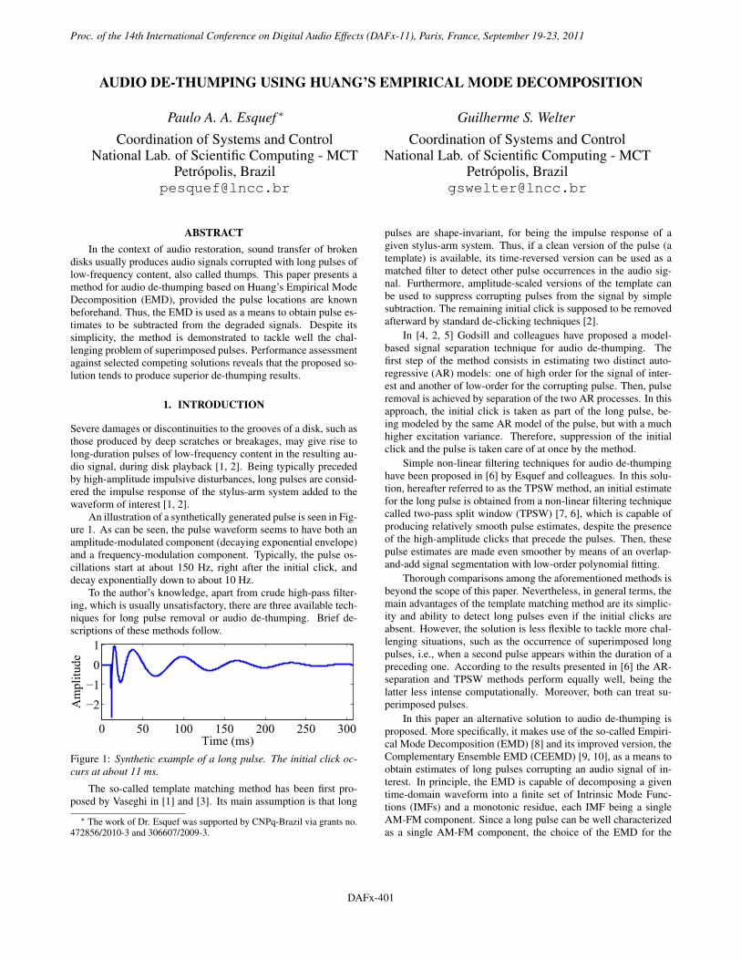
Severe damages or discontinuities to the grooves of a disk, such asthose produced by deep scratches or breakages, may give rise tolong-duration pulses of low-frequency content in the resulting au-dio signal, during disk playback [1, 2]. Being typically precededby high-amplitude impulsive disturbances, long pulses are consid-ered the impulse response of the stylus-arm system added to thewaveform of interest [1, 2].

An illustration of a synthetically generated pulse is seen in Fig-ure 1. As can be seen, the pulse waveform seems to have both anamplitude-modulated component (decaying exponential envelope)and a frequency-modulation component. Typically, the pulse os-cillations start at about 150 Hz, right after the initial click, anddecay exponentially down to about 10 Hz.

To the author’s knowledge, apart from crude high-pass filter-ing, which is usually unsatisfactory, there are three available tech-niques for long pulse removal or audio de-thumping. Brief de-scriptions of these methods follow.

0 50 100 150 200 250 300

−2

−1

0

1

Time (ms)

Am

pli

tud

e

Figure 1: Synthetic example of a long pulse. The initial click oc-curs at about 11 ms.

The so-called template matching method has been first pro-posed by Vaseghi in [1] and [3]. Its main assumption is that long

∗ The work of Dr. Esquef was supported by CNPq-Brazil via grants no.472856/2010-3 and 306607/2009-3.

pulses are shape-invariant, for being the impulse response of agiven stylus-arm system. Thus, if a clean version of the pulse (atemplate) is available, its time-reversed version can be used as amatched filter to detect other pulse occurrences in the audio sig-nal. Furthermore, amplitude-scaled versions of the template canbe used to suppress corrupting pulses from the signal by simplesubtraction. The remaining initial click is supposed to be removedafterward by standard de-clicking techniques [2].

In [4, 2, 5] Godsill and colleagues have proposed a model-based signal separation technique for audio de-thumping. Thefirst step of the method consists in estimating two distinct auto-regressive (AR) models: one of high order for the signal of inter-est and another of low-order for the corrupting pulse. Then, pulseremoval is achieved by separation of the two AR processes. In thisapproach, the initial click is taken as part of the long pulse, be-ing modeled by the same AR model of the pulse, but with a muchhigher excitation variance. Therefore, suppression of the initialclick and the pulse is taken care of at once by the method.

Simple non-linear filtering techniques for audio de-thumpinghave been proposed in [6] by Esquef and colleagues. In this solu-tion, hereafter referred to as the TPSW method, an initial estimatefor the long pulse is obtained from a non-linear filtering techniquecalled two-pass split window (TPSW) [7, 6], which is capable ofproducing relatively smooth pulse estimates, despite the presenceof the high-amplitude clicks that precede the pulses. Then, thesepulse estimates are made even smoother by means of an overlap-and-add signal segmentation with low-order polynomial fitting.

Thorough comparisons among the aforementioned methods isbeyond the scope of this paper. Nevertheless, in general terms, themain advantages of the template matching method are its simplic-ity and ability to detect long pulses even if the initial clicks areabsent. However, the solution is less flexible to tackle more chal-lenging situations, such as the occurrence of superimposed longpulses, i.e., when a second pulse appears within the duration of apreceding one. According to the results presented in [6] the AR-separation and TPSW methods perform equally well, being thelatter less intense computationally. Moreover, both can treat su-perimposed pulses.

In this paper an alternative solution to audio de-thumping isproposed. More specifically, it makes use of the so-called Empiri-cal Mode Decomposition (EMD) [8] and its improved version, theComplementary Ensemble EMD (CEEMD) [9, 10], as a means toobtain estimates of long pulses corrupting an audio signal of in-terest. In principle, the EMD is capable of decomposing a giventime-domain waveform into a finite set of Intrinsic Mode Func-tions (IMFs) and a monotonic residue, each IMF being a singleAM-FM component. Since a long pulse can be well characterizedas a single AM-FM component, the choice of the EMD for the

DAFX-1

Proc. of the 14th International Conference on Digital Audio Effects (DAFx-11), Paris, France, September 19-23, 2011

DAFx-401


problem at hand seems justified.The experimental results reported in this paper reveal that the

EMD and the CEEMD are effective and simple tools to provideadequate pulse estimates. Performance evaluation of the proposedmethod against the AR-separation and TPSW methods is carriedout via the Perceptual Audio Quality Measure (PAQM) [11]. Theattained results show that the CEEMD-based audio de-thumpingperforms comparably to the competing solutions.

The remainder of the paper is organized as follows. In Sec-tion 2 brief reviews of the EMD and the CEEMD are given. Theproposed pulse estimation method is explained in Section 3. Theexperimental setup defined for the comparative tests is describedin Section 4. In Section 4.3 the attained results are presented anddiscussed. Finally, conclusions are drawn in Section 5.

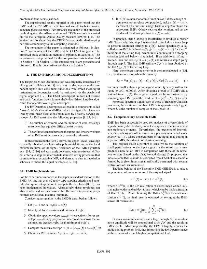
2. THE EMPIRICAL MODE DECOMPOSITION

The Empirical Mode Decomposition was originally introduced byHuang and collaborators [8] as a way to decompose multicom-ponent signals into constituent functions from which meaningfulinstantaneous frequencies could be estimated via the AnalyticalSignal approach [12]. The EMD decomposition does not assumeany basis function since it is an entirely data-driven iterative algo-rithm that operates over signal envelopes.

The EMD method decomposes a signal into components calledIntrinsic Mode Functions (IMFs), which are typically character-ized by zero-mean oscillations modulated by a slowly varying en-velope. An IMF must have the following properties [8, 13, 14]:

1. The number of extrema and the number of zero-crossingsmust be either equal or differ at most by one;

2. The arithmetic mean between the upper and lower envelopesof an IMF must be zero at any point of its domain.

With reference to the item 2 above, the upper (lower) envelopeis usually obtained via low-order polynomial fitting to the localmaxima (minima) of the signal. Variations on the EMD algorithmexist [14, 15, 16] and are mainly concerned with two issues: differ-ent criteria to stop the intermediate iterative sifting procedure thatculminate in an acceptable IMF; and alternative data extrapolationschemes to obtain the signal envelopes [17, 10].

2.1. EMD Implementation

For the experiments reported in the paper, a standard version of theEMD, i.e., one that uses a Cauchy-type stopping criterion and natu-ral cubic spline interpolation to compute the envelopes [8, 13], hasbeen implemented in Matlab. Alternatively, these envelopes canalso be obtained via piecewise cubic Hermite interpolating poly-nomials across local maxima (minima).

Considering a signal x(t), the EMD is described as follows.

1. Let j = 1 and set xj(t) = x(t);

2. Identify all local maxima and minima of xj(t);

3. Obtain the upper envelope eupper(t) (respectively, lower en-velope elower(t)) by polynomial interpolation across the lo-cal maxima (respectively, local minima) of xj(t) ;

4. Compute the mean envelope m(t) =[eupper(t)+elower(t)

]/2;

5. Obtain an IMF estimate Cj(t) = xj(t) − m(t);

6. If m(t) is a non-monotonic function (or if it has enough ex-trema to allow envelope computation), make xj(t) = m(t);increment j by one unit; and go back to step 2 to obtain thesubsequent IMFs. Otherwise, stop the iterations and set theresidue of the decomposition as r(t) = m(t).

In practice, step 5 above is insufficient to produce a properIMF. To remedy this, step 5 is modified to include an inner loopto perform additional siftings to xj(t). More specifically, a so-called proto-IMF is defined as Cj,k(t) = xj(t)−m(t) for the kth

iteration of the sifting loop, which must continue until a stoppingcriterion (defined below) is satisfied. If an additional sifting isneeded, then one sets xj(t) = Cj,k(t) and returns to step 2 goingthrough step 5. The final IMF estimate Cj(t) is then obtained asthe last Cj,k(t) of the sifting loop.

Here, the chosen stoping criterion is the same adopted in [13],i.e., the iterations stop when the quantity

Sd = Var{Cj,k−1(t) − Cj,k(t)

}/Var

{Cj,k−1(t)

}(1)

becomes smaller than a pre-assigned value, typically within therange [0.0001–0.0003]. After obtaining a total of J IMFs and aresidual trend rJ(t), the original signal can be reconstructed bysumming up all IMFs and the trend: x(t) =

∑Jj=1 Cj(t)+rJ(t).

For broad spectrum signals such as those of fractal or Gaussianprocesses, the maximum number of IMFs is approximately log2 L,where L is the number of samples of the signal [18].

2.2. Complementary Ensemble EMD

EMD has been successfully used for analysis of diverse kinds ofsignals, mainly due its ability to tackle responses of non-linear andnon-stationary systems. Nevertheless, the presence of intermit-tency in such signals often results in a phenomenon called modemixing [13, 14], where coherent parts of the signal may end up inadjacent IMFs, thus devoid of physical meaning.

The original EMD algorithm is sensitive to the addition ofsmall perturbations to the input signal, in the sense that it mayproduce a new set of IMFs in comparison with those of the noise-less version. Based on this fact, Wu and Huang [10] proposed thatmore reliable IMFs should be estimated from EMD of an ensembleformed by a given input signal artificially corrupted with severalrealizations of Gaussian noise.

The idea behind of the Ensemble EMD (EEMD) is to take alarge number of noisy versions of the original signal

x(i)(t) = x(t) + ε w(i)(t), (2)

where ε w(i)(t) is the i-th realization of a zero-mean white Gaus-sian noise with standard deviation ε, which can be made a fractionof that of x(t). After obtaining the IMFs C

(i)j (t) for each real-

ization x(i)(t), the final result is obtained by averaging the IMFsacross all realizations:

C̃j(t) = limN→∞

1

N

N∑

i=1

C(i)j (t). (3)

Given a non-infinitesimal ε and a large enough N , the residualnoise amplitude will be proportional to ε/

√N and the resulting

IMFs stable. More importantly, the EEMD largely reduces themode mixing problem [10], thus improving the EMD performanceat the expense of a much higher computational load.

DAFX-2


DAFx-402


A further improvement to the EEMD is the ComplementaryEEMD (CEEMD), in which the ensemble is formed by N/2 com-plementary pairs of noise realizations with symmetric amplitude.This way, Eq. (2) is modified to x(i)(t) = x(t)+(−1)iε w(i−γ)(t),for i = 1, 2, . . . , N , where γ = i modulo 2. The IMFs of the thusconstructed ensemble are then obtained as before via Eq. (3). Thisprocedure ensures that the residual noise will be zero.

3. LONG PULSE ESTIMATION VIA EMD AND CEEMD

Similar to the AR-separation and TPSW methods, the proposedEMD-based de-thumping requires prior knowledge of pulse loca-tions in time. This means that, for a particular pulse, estimatesof its onset time and duration must be available. In practice, theformer can be inferred from the location of the initial click, whichcan easily obtained by standard detection techniques [2].

From the auditory perception perspective, the most salient partof a long pulse is its beginning, for its higher amplitude and fre-quency. Therefore, pulse duration estimates can be obtained byvisual inspection. In other words, underestimation of pulse dura-tions is likely to produce no audible effects.

3.1. EMD-based Estimation of Single Pulses

For didactic reasons, EMD-based estimation of single pulses ispresented first, being that of superimposed pulses left to later.

The main steps of the pulse estimation procedure (one pulseat a time) are listed below. More specific details of each step aregiven in the sequel.

1. Select a portion of the signal of interest containing one sin-gle long pulse (to be called input signal hereafter);

2. Extend the input signal backward in time;

3. Analyze the extended input signal via the EMD. The mainparameter to be defined is the maximum number of IMFs.

4. Form the pulse estimate by mixing together partial recon-structions of the signal, with different levels of detail, viaan overlap-and-add windowing scheme.

As regards step 1, the beginning of the input signal shouldcoincide with that of the pulse, i.e., it should start right after theinitial click. The duration of the segment should be approximatelythat of the observed long pulse. It is advisable though to add about5 ms to the duration in order to overcome boundary effects thatmay affect IMF estimation [17, 10]. For that very reason, step 2is taken. The idea here is to analyze an input signal a bit longerthan necessary and then discard samples at the extremities of theensuing IMFs and residue to get rid of possible boundary effects.Therefore, the backward signal extrapolation carried out in step 2does not need to be much involved. It can be simple enough to justcapture the tendency of the signal trajectory.

Signal extension backward in time should be made for at leastthe duration of the initial click. For that, extrapolation schemesbased on AR modeling [2, 19] can be used. A simpler solution,which is employed here, consists in mirroring the beginning of theinput signal with odd symmetry w.r.t. its first sample.

The EMD in step 3 uses a standard version of the algorithm(see Section 2.1). As for the treatment of envelope boundaries, thesolution proposed in [10] is resorted to. More specifically, consid-ering the upper envelope for didactic reasons, a straight line is firstfitted to the two consecutive maxima nearest to the end (or begin-ning) of the signal. Then, an artificial new end (or beginning) point

for the envelope is created at the end (or beginning) of the segment.This new point is taken as the largest value between the own signaland the linearly extrapolated envelope. A similar scheme can beemployed to extend the lower envelope. In both cases, no exten-sion of the input signal is carried out, just extrapolation of its lowerand upper envelopes toward its boundaries.

The aforementioned procedure surely helps to reduce end ef-fects observed in the IMFs, but do not completely eliminate them.Hence, input signal extrapolation performed in step 2 is still needed.

One of the known issues of the standard EMD is the so-calledmode-mixing or intermittence [8], which consists of the split of anapparent single intrinsic mode between two adjacent IMFs. Intrin-sic mode segregation is a complex question whose discussion isbeyond the scope of this paper. As reported in [20] it depends onparameters such as the relative amplitude of the modes and theirproximity in frequency.

As one could anticipate from the above discussion, although asingle long pulse would qualify for being an IMF, it is not alwaystrue that one of the IMFs produced by EMD of the input signalconstitutes alone an adequate pulse estimate. The main reason forthat seems to be the overlap between the spectral range of the longpulse and the low-frequency content of the audio signal of interest.

An illustration of the mode-mixing problem in the context ofEMD-based pulse estimation is depicted in Figure 2. As can beseen, while the tail of the pulse is well captured by the residueobtained after extracting seven IMFs, adequate representation ofthe initial faster oscillations only happens if the 7th IMF is addedto the residue.

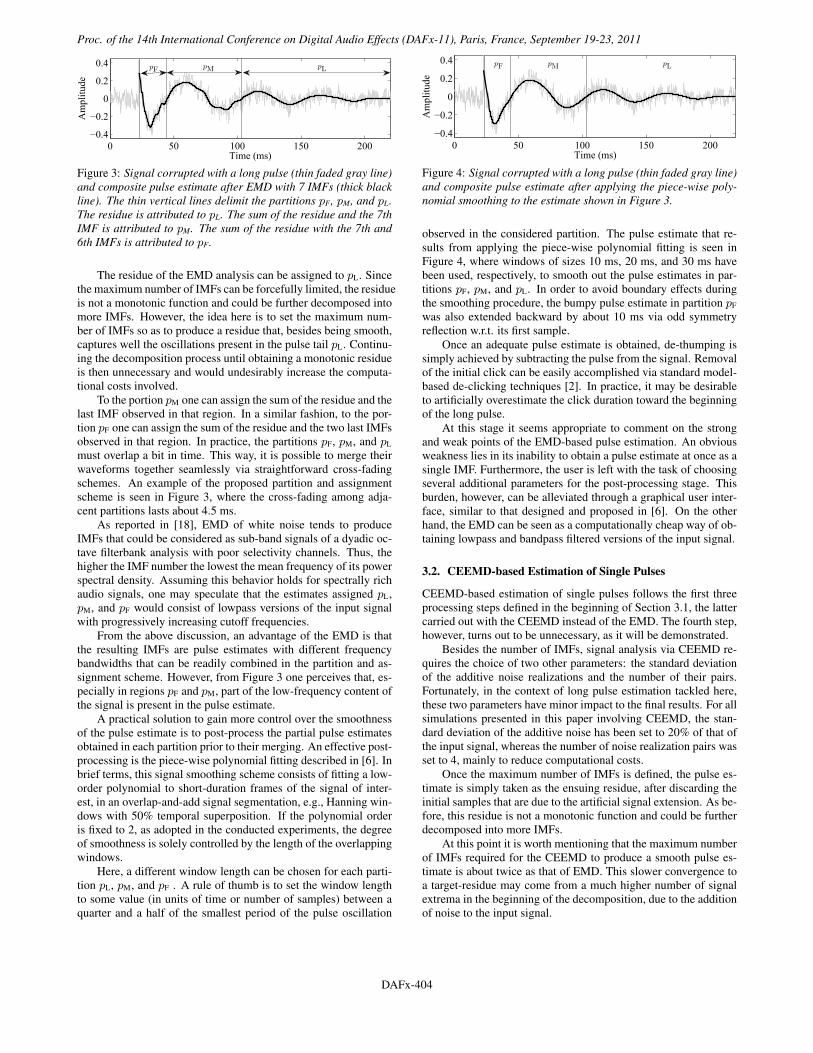
Similar to the strategy employed in [6], a practical way to ob-tain a useful pulse estimate is to predefine three temporal regionsfor the pulse and assign to each region pulse estimates with dif-ferent degrees of detail (or frequency ranges). One pulse partitionthat typically works in practice is the following:

pF: about half oscillation cycle from the beginning of the pulse;

pM: about one and half oscillation cycles from the end of pF;

pL: the rest of the pulse from the end of pM.

0 50 100 150 200−0.4

−0.2

0

0.2

0.4

Am

pli

tud

e

0 50 100 150 200−0.4

−0.2

0

0.2

0.4

Am

pli

tud

e

0 50 100 150 200−0.4

−0.2

0

0.2

0.4

Am

pli

tud

e

Time (ms)

Figure 2: Top: Signal corrupted with a long pulse. The thin verti-cal line at about 25 ms indicates the beginning of the pulse. Mid-dle: corrupted signal (thin faded gray line) and residue after ex-tracting the first 7 IMFs (thick black line). Bottom: corruptedsignal (thin faded gray line) and the sum of the residue with the7th IMF (thick black line).

DAFX-3


DAFx-403


0 50 100 150 200

−0.4

−0.2

0

0.2

0.4

Time (ms)

Am

pli

tud

e

pFpM pL

Figure 3: Signal corrupted with a long pulse (thin faded gray line)and composite pulse estimate after EMD with 7 IMFs (thick blackline). The thin vertical lines delimit the partitions pF, pM, and pL.The residue is attributed to pL. The sum of the residue and the 7thIMF is attributed to pM. The sum of the residue with the 7th and6th IMFs is attributed to pF.

The residue of the EMD analysis can be assigned to pL. Sincethe maximum number of IMFs can be forcefully limited, the residueis not a monotonic function and could be further decomposed intomore IMFs. However, the idea here is to set the maximum num-ber of IMFs so as to produce a residue that, besides being smooth,captures well the oscillations present in the pulse tail pL. Continu-ing the decomposition process until obtaining a monotonic residueis then unnecessary and would undesirably increase the computa-tional costs involved.

To the portion pM one can assign the sum of the residue and thelast IMF observed in that region. In a similar fashion, to the por-tion pF one can assign the sum of the residue and the two last IMFsobserved in that region. In practice, the partitions pF, pM, and pL

must overlap a bit in time. This way, it is possible to merge theirwaveforms together seamlessly via straightforward cross-fadingschemes. An example of the proposed partition and assignmentscheme is seen in Figure 3, where the cross-fading among adja-cent partitions lasts about 4.5 ms.

As reported in [18], EMD of white noise tends to produceIMFs that could be considered as sub-band signals of a dyadic oc-tave filterbank analysis with poor selectivity channels. Thus, thehigher the IMF number the lowest the mean frequency of its powerspectral density. Assuming this behavior holds for spectrally richaudio signals, one may speculate that the estimates assigned pL,pM, and pF would consist of lowpass versions of the input signalwith progressively increasing cutoff frequencies.

From the above discussion, an advantage of the EMD is thatthe resulting IMFs are pulse estimates with different frequencybandwidths that can be readily combined in the partition and as-signment scheme. However, from Figure 3 one perceives that, es-pecially in regions pF and pM, part of the low-frequency content ofthe signal is present in the pulse estimate.

A practical solution to gain more control over the smoothnessof the pulse estimate is to post-process the partial pulse estimatesobtained in each partition prior to their merging. An effective post-processing is the piece-wise polynomial fitting described in [6]. Inbrief terms, this signal smoothing scheme consists of fitting a low-order polynomial to short-duration frames of the signal of inter-est, in an overlap-and-add signal segmentation, e.g., Hanning win-dows with 50% temporal superposition. If the polynomial orderis fixed to 2, as adopted in the conducted experiments, the degreeof smoothness is solely controlled by the length of the overlappingwindows.

Here, a different window length can be chosen for each parti-tion pL, pM, and pF . A rule of thumb is to set the window lengthto some value (in units of time or number of samples) between aquarter and a half of the smallest period of the pulse oscillation

0 50 100 150 200

−0.4

−0.2

0

0.2

0.4

Time (ms)

Am

pli

tud

e

pF pM pL

Figure 4: Signal corrupted with a long pulse (thin faded gray line)and composite pulse estimate after applying the piece-wise poly-nomial smoothing to the estimate shown in Figure 3.

observed in the considered partition. The pulse estimate that re-sults from applying the piece-wise polynomial fitting is seen inFigure 4, where windows of sizes 10 ms, 20 ms, and 30 ms havebeen used, respectively, to smooth out the pulse estimates in par-titions pF, pM, and pL. In order to avoid boundary effects duringthe smoothing procedure, the bumpy pulse estimate in partition pF

was also extended backward by about 10 ms via odd symmetryreflection w.r.t. its first sample.

Once an adequate pulse estimate is obtained, de-thumping issimply achieved by subtracting the pulse from the signal. Removalof the initial click can be easily accomplished via standard model-based de-clicking techniques [2]. In practice, it may be desirableto artificially overestimate the click duration toward the beginningof the long pulse.

At this stage it seems appropriate to comment on the strongand weak points of the EMD-based pulse estimation. An obviousweakness lies in its inability to obtain a pulse estimate at once as asingle IMF. Furthermore, the user is left with the task of choosingseveral additional parameters for the post-processing stage. Thisburden, however, can be alleviated through a graphical user inter-face, similar to that designed and proposed in [6]. On the otherhand, the EMD can be seen as a computationally cheap way of ob-taining lowpass and bandpass filtered versions of the input signal.

3.2. CEEMD-based Estimation of Single Pulses

CEEMD-based estimation of single pulses follows the first threeprocessing steps defined in the beginning of Section 3.1, the lattercarried out with the CEEMD instead of the EMD. The fourth step,however, turns out to be unnecessary, as it will be demonstrated.

Besides the number of IMFs, signal analysis via CEEMD re-quires the choice of two other parameters: the standard deviationof the additive noise realizations and the number of their pairs.Fortunately, in the context of long pulse estimation tackled here,these two parameters have minor impact to the final results. For allsimulations presented in this paper involving CEEMD, the stan-dard deviation of the additive noise has been set to 20% of that ofthe input signal, whereas the number of noise realization pairs wasset to 4, mainly to reduce computational costs.

Once the maximum number of IMFs is defined, the pulse es-timate is simply taken as the ensuing residue, after discarding theinitial samples that are due to the artificial signal extension. As be-fore, this residue is not a monotonic function and could be furtherdecomposed into more IMFs.

At this point it is worth mentioning that the maximum numberof IMFs required for the CEEMD to produce a smooth pulse es-timate is about twice as that of EMD. This slower convergence toa target-residue may come from a much higher number of signalextrema in the beginning of the decomposition, due to the additionof noise to the input signal.

DAFX-4


DAFx-404


0 50 100 150 200

−0.4

−0.2

0

0.2

0.4

Time (ms)

Am

pli

tud

e

Figure 5: Signal corrupted with a long pulse (thin faded gray line)and pulse estimate (thick black line) as the CEEMD residue afterextracting the first 12 IMFs. The thin vertical line at about 23 msindicates the actual beginning of the pulse. Pulse samples beforethat limit should be discarded.

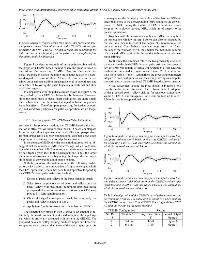
Figure 5 displays an example of pulse estimate obtained viathe proposed CEEMD-based method, where the pulse is taken asthe residue after extracting 12 IMFs. Here, for illustration pur-poses, the pulse is plotted including the samples related to a back-ward signal extension of about 2.5 ms. As can be seen, the at-tained pulse estimate exhibits an adequate level of smoothness andis capable of following the pulse trajectory in both fast and slowoscillation regions.

In comparison with the pulse estimate shown in Figure 4, theone yielded by the CEEMD solution is a bit bumpier. However,since the amplitudes of these faster oscillations are quite small,their subtraction from the corrupted signal is bound to produceinaudible effects. Therefore, post-processing for further smooth-ing and windowing schemes for pulse composition are no longerneeded.

3.2.1. Speeding up the CEEMD-Based Pulse Estimation

As seen in the previous section, the CEEMD-based pulse esti-mation is effective, yet simpler than the EMD-based counterpart,from the algorithm implementation and calibration perspectives.Its main drawback is a higher computational cost that slows downthe process of obtaining the desired pulse estimates.

In the context of EMD of white noise, findings reported in [18]suggest that the number of IMF zero-crossings, which holds rela-tion with the number of IMF extrema, tends to decrease on averageby half from a given IMF to the subsequent one. Thus, the largerthe number of extrema in the beginning, the longer the decompo-sition takes to converge to a monotonic residue.

With the previous information in mind, the following modifi-cation, which affects the computation of signal envelopes withinthe EEMD processing chain, has been found operative to speed upthe CEEMD-based pulse estimation method:

1. Detect all peaks and valleys of the input signal as usual;

2. Select from the previous set of peaks and valleys only thepeak (valley) with maximum (minimum) amplitude insidejuxtaposed observation windows of 3.4 ms (about 150 sam-ples at 44.1 kHz sampling rate);

3. Obtain the signal envelopes as usual, but using only thepeaks and valleys selected in step 2;

4. Apply item 2 only for extraction of the first two IMFs.

The selection performed in step 2 above is an attempt to re-tain only the most prominent peaks and valleys of the input sig-nal, which is artificially corrupted with noise in the CEEMD. Theproposed peak and valley pruning produces upper and lower en-velopes are way smoother than those of the noisy input signal. As

a consequence, the frequency bandwidths of the first two IMFs arelarger than those of the corresponding IMFs computed via conven-tional CEEMD, forcing the modified CEEMD iterations to con-verge faster to slowly varying IMFs, which are of interest to thepresent application.

Together with the maximum number of IMFs, the length ofthe observation window in step 2 above can also be changed bythe user as a means to control the degree of smoothness of thepulse estimate. Considering a practical range from 1 to 10 ms,the longer the window length, the smaller the maximum numberof extracted IMFs required for the residue to become an adequatepulse estimate.

To illustrate the combined role of the two previously discussedparameters in the final CEEMD-based pulse estimate, outcomes oftwo different yet equally effective configurations of the CEEMDmethod are presented in Figure 6 and Figure 7. In connectionwith these results, Table 1 summarizes the processing parametersadopted in each configuration and the average savings in computa-tional time w.r.t the conventional CEEMD-based pulse estimation.

Visual assessment among the plots shown in Figures 5 to 7reveals similar pulse estimates. Hence, from Table 1, adoptionof the proposed peak (valley) picking for envelope computationwithin CEEMD is advantageous, for it can produce up to a ten-fold reduction in computational time.

0 50 100 150 200

−0.4

−0.2

0

0.2

0.4

Time (ms)

Am

pli

tud

e

Figure 6: Signal corrupted with a long pulse (thin faded gray line)and pulse estimate (thick black line) as the CEEMD residue af-ter extracting 4 IMFs. Peak and valley selection was carried outwithin juxtaposed windows of 3.4 ms.

0 50 100 150 200

−0.4

−0.2

0

0.2

0.4

Time (ms)

Am

pli

tud

e

Figure 7: Signal corrupted with a long pulse (thin faded gray line)and pulse estimate (thick black line) as the CEEMD residue afterextracting only 2 IMFs. Peak and valley selection was carried outwithin juxtaposed windows of 6.8 ms.

Table 1: Configuration of the CEEMD-based pulse estimation andcorresponding results. The value of T is about 10 s when runningthe CEEMD analysis on a Core i7 870 2.93 GHz Quad Core CPU.All simulations ran on the same machine.

CEEMD Configuration ResultsNo. IMFs Window Size Avg. Proc. Time Visual Output

13 – T Figure 54 3.4 ms T/3.8 Figure 62 6.8 ms T/10 Figure 7

DAFX-5


DAFx-405


3.2.2. A Real-World Example of CEEMD-based De-Thumping

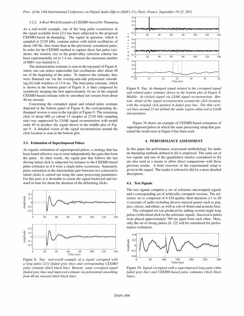
As a real-world example, one of the long pulse occurrences inthe signal available from [21] has been subjected to the proposedCEEMD-based de-thumping. The signal in question, which issampled at 22.05 kHz, contains pulses with initial oscillations ofabout 180 Hz, thus faster than in the previously considered pulse.In order for the CEEMD method to capture those fast pulse vari-ations, the window size in the peak/valley selection scheme hasbeen experimentally set to 1.4 ms, whereas the maximum numberof IMFs was limited to 2.

The attained pulse estimate is seen in the top panel of Figure 8,where one can notice undesirable fast oscillations after about 40ms of the beginning of the pulse. To improve the estimate, theywere flattened out via the overlap-and-add polynomial smooth-ing [6] with windows of 13.6 ms. The final pulse estimate, whichis shown in the bottom panel of Figure 8, is then composed byseamlessly merging the first approximately 16 ms of the originalCEEMD-based estimate with its smoothed out version from about40 ms onward.

Concerning the corrupted signal and related pulse estimatedepicted in the bottom panel of Figure 8, the corresponding de-thumped version is seen in the top plot of Figure 9. The remainingclick of about 680 µs (about 15 samples at 22.05 kHz samplingrate) was suppressed by LSAR signal reconstruction with modelorder 65 to produce the signal shown in the middle plot of Fig-ure 9. A detailed vision of the signal reconstruction around theclick location is seen in the bottom plot.

3.3. Estimation of Superimposed Pulses

As regards estimation of superimposed pulses, a strategy that hasbeen found effective was to treat independently the parts that formthe pulse. In other words, the signal part that follows the lastdriving initial click is subjected for instance to the CEEMD-basedpulse estimator as if it were a single pulse occurrence. Separately,pulse estimation in the intermediate part between two consecutiveinitial clicks is carried out using the same processing parameters.For this part, it is desirable to extent the signal backward and for-ward in time for about the duration of the delimiting clicks.

0 20 40 60 80 100 120 140

−0.2

−0.1

0

0.1

0.2

Am

pli

tud

e

0 20 40 60 80 100 120 140

−0.2

−0.1

0

0.1

0.2

Time (ms)

Am

pli

tud

e

Figure 8: Top: real-world example of a signal corrupted witha long pulse [21] (faded gray line) and corresponding CEEMDpulse estimate (thick black line). Bottom: same corrupted signal(faded gray line) and improved estimate via polynomial smoothingfrom 40 ms onward (thick black line).

0 20 40 60 80 100 120 140−0.2

0

0.2

0.4

0.6

0 20 40 60 80 100 120 140−0.2

0

0.2

0.4

0.6

A m

p

l

i

t

u

d

e

20 21 22 23 24 25 26−0.2

0

0.2

0.4

0.6

Time (ms)

Figure 9: Top: de-thumped signal related to the corrupted signaland related pulse estimate shown in the bottom plot of Figure 8.Middle: de-clicked signal via LSAR signal reconstruction. Bot-tom: detail of the signal reconstruction around the click location,with the original click painted in faded gray line. The thin verti-cal lines around 23 ms delimit the audio region subjected to LSARinterpolation.

Figure 10 shows an example of CEEMD-based estimation ofsuperimposed pulses in which the same processing setup that gen-erated the result seen in Figure 6 has been used.

4. PERFORMANCE ASSESSMENT

In this paper the performance assessment methodology for audiode-thumping methods defined in [6] is employed. The same set oftest signals and one of the quantitative metrics considered in [6]are also used as a means to allow direct comparisons with thoseprevious results. A brief overview of the experimental setup isgiven in the sequel. The reader is referred to [6] for a more detaileddescription.

4.1. Test Signals

The test signals comprise a set of reference uncorrupted signalsand a corresponding set of artificially corrupted versions. The ref-erence set is composed of 6 CD-quality short-duration (11 to 20s) excerpts of audio including diverse musical genres such as pop,jazz, classic, and ethnic, as well as solo of drums and acoustic bass.

The corrupted set was produced by adding several single longpulses (with initial click) to the reference signals. Successive pulseswere placed approximately 769 ms apart from each other. Here,only the set of strong pulses [6, 22] will be considered for perfor-mance evaluation.

0 50 100 150 200 250 300

−0.4

−0.2

0

0.2

0.4

Time (ms)

Am

pli

tud

e

Figure 10: Signal corrupted with a superimposed long pulse (thinfaded gray line) and CEEMD-based pulse estimates (thick blacklines).

DAFX-6


DAFx-406


4.2. Experimental Setup and Performance Metric

As in [6], the evaluation methodology adopted here consists infirst obtaining restored versions (de-thumped and de-clicked) ofthe corrupted set via a selection of de-thumping methods with pre-defined configurations. Then, the reference and restored sets arecompared by objective means.

Here, the Perceptual Audio Quality Measure (PAQM) [11] isused as the performance metric. In a nutshell, the PAQM comparesa processed signal w.r.t. a reference and outputs a dissimilarity in-dex that takes into account several properties of the human audi-tory system, such as masking in time and frequency. The closerto zero the PAQM, the more similar perceptually are the processedand reference signals.

The aim here is to run a direct comparison among the PAQMvalues associated with the restored signals produced by the follow-ing de-thumping methods: AR Separation (ARS), TPSW-based(TPSW), EMD-based pulse estimation (EMD), and CEEMD-basedpulse estimation (CEEMD). Therefore, only the processing setupof the EMD and the CEEMD will be defined. The processing pa-rameters employed in the ARS and the TPSW can be found in [6].

4.2.1. EMD Configuration

The following configuration was employed to obtain the EMD-related results:

• Backward signal extension: 100 samples with odd symme-try w.r.t. the first sample;

• Maximum number of IMFs: 6;

• Envelope computation: piecewise cubic Hermite interpolat-ing polynomials across local maxima (minima);

• pF: 44 ms from the beginning of the pulse;

• pM: 60 ms from the end of pF;

• pL: 100 ms from the end of pM;

• Pulse estimate inside pF: (residue + 6th IMF + 5th IMF)smoothed out via the overlap-and-add polynomial schemewith windows of 10 ms and 2nd-order polynomials;

• Pulse estimate inside pM: (residue + 6th IMF) smoothed outvia the overlap-and-add polynomial scheme with windowsof 20 ms and 2nd-order polynomials;

• Pulse estimate inside pL: (residue) smoothed out via theoverlap-and-add polynomial scheme with windows of 30ms and 2nd-order polynomials;

• Click removal: 75th-order LSAR signal reconstruction of50 samples from the click onset.

4.2.2. CEEMD Configuration

The following configuration was employed to obtain the CEEMD-related results:

• Number of noise realization pairs: N/2 = 4;

• Standard deviation of each realization: ε = 0.2 std{x(t)};

• Backward signal extension: 100 samples with odd symme-try w.r.t. the first sample;

• Maximum number of IMFs: 4;

• Envelope computation (for first two IMFs): piecewise cu-bic Hermite interpolating polynomials across local maxima(minima), after selection of one maximum (minimum) perjuxtaposed windows of 3.4 ms;

• Envelope computation (third and fourth IMFs): piecewisecubic Hermite interpolating polynomials across local max-ima (minima);

• Click removal: 75th-order LSAR signal reconstruction of50 samples from the click onset.

4.3. Results and Discussion

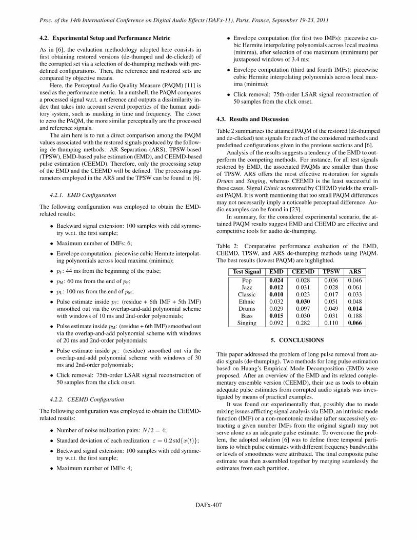
Table 2 summarizes the attained PAQM of the restored (de-thumpedand de-clicked) test signals for each of the considered methods andpredefined configurations given in the previous sections and [6].

Analysis of the results suggests a tendency of the EMD to out-perform the competing methods. For instance, for all test signalsrestored by EMD, the associated PAQMs are smaller than thoseof TPSW. ARS offers the most effective restoration for signalsDrums and Singing, whereas CEEMD is the least successful inthese cases. Signal Ethnic as restored by CEEMD yields the small-est PAQM. It is worth mentioning that too small PAQM differencesmay not necessarily imply a noticeable perceptual difference. Au-dio examples can be found in [23].

In summary, for the considered experimental scenario, the at-tained PAQM results suggest EMD and CEEMD are effective andcompetitive tools for audio de-thumping.

Table 2: Comparative performance evaluation of the EMD,CEEMD, TPSW, and ARS de-thumping methods using PAQM.The best results (lowest PAQM) are highlighted.

Test Signal EMD CEEMD TPSW ARSPop 0.024 0.028 0.036 0.046Jazz 0.012 0.031 0.028 0.061

Classic 0.010 0.023 0.017 0.033Ethnic 0.032 0.030 0.051 0.048Drums 0.029 0.097 0.049 0.014Bass 0.015 0.030 0.031 0.188

Singing 0.092 0.282 0.110 0.066

5. CONCLUSIONS

This paper addressed the problem of long pulse removal from au-dio signals (de-thumping). Two methods for long pulse estimationbased on Huang’s Empirical Mode Decomposition (EMD) wereproposed. After an overview of the EMD and its related comple-mentary ensemble version (CEEMD), their use as tools to obtainadequate pulse estimates from corrupted audio signals was inves-tigated by means of practical examples.

It was found out experimentally that, possibly due to modemixing issues afflicting signal analysis via EMD, an intrinsic modefunction (IMF) or a non-monotonic residue (after successively ex-tracting a given number IMFs from the original signal) may notserve alone as an adequate pulse estimate. To overcome the prob-lem, the adopted solution [6] was to define three temporal parti-tions to which pulse estimates with different frequency bandwidthsor levels of smoothness were attributed. The final composite pulseestimate was then assembled together by merging seamlessly theestimates from each partition.

DAFX-7


DAFx-407


As regards signal analysis via the CEEMD, it was discov-ered that adequate pulse estimates could be obtained at once as anon-monotonic residue after successively extracting a given num-ber IMFs from the original signal. However, as compared withthe EMD, about twice the number of initial IMFs needed to beextracted for producing a smooth enough pulse estimate. OtherCEEMD parameters such as the variance of the additive noise andthe number of ensemble pairs had negligible impact on the finalresults. As a means to decrease the computational cost of theCEEMD for the studied application, a modified scheme for sig-nal envelope computation was devised: piecewise cubic Hermiteinterpolating polynomials were fitted across local maxima (min-ima), after selection of one maximum (minimum) per juxtaposedshort-duration windows. Average reductions in computation timeup to ten times were reported.

Objective performance evaluation of the proposed EMD- andCEEMD-based methods for audio de-thumping was carried out us-ing the same methodology and test data of [6]. Indirect compara-tive results, in terms of the Perceptual Audio Quality Measure [11]of the restored versions of the corrupted data, suggest the proposedCEEMD-based method tends to perform as effectively as the com-peting TPSW-based procedure [6] and outperform the AR separa-tion method [2]. As regards the EMD-based method the observedtendency is of a more favorably performance in comparison withthe TPSW-based solution.

6. REFERENCES

[1] S. V. Vaseghi, Algorithms for Restoration of ArchivedGramophone Recordings, Ph.D. thesis, Cambridge Univ.,UK, 1988.

[2] S. J. Godsill and P. J. W. Rayner, Digital Audio Restoration— A Statistical Model Based Approach, Springer-Verlag,London, UK, 1998.

[3] S. V. Vaseghi and R. Frayling-Cork, “Restoration of OldGramophone Recordings,” J. Audio Eng. Soc., vol. 40, no.10, pp. 791–801, Oct. 1992.

[4] S. J. Godsill, The Restoration of Degraded Audio Signals,Ph.D. thesis, Cambridge Univ., UK, 1993.

[5] S. J. Godsill and C. H. Tan, “Removal of Low FrequencyTransient Noise from Old Recordings Using Model-BasedSignal Separation Techniques,” in Proc. IEEE WASPAA,1997.

[6] P. A. A. Esquef, L. W. P. Biscainho, and V. Välimäki, “An Ef-ficient Algorithm for the Restoration of Audio Signals Cor-rupted with Low-Frequency Pulses,” J. Audio Eng. Soc., vol.51, no. 6, pp. 502–517, June 2003.

[7] W. A. Struzinski and E. D. Lowe, “A Performance Compari-son of Four Noise Background Normalization Schemes Pro-posed for Signal Detection Systems,” J. Acoust. Soc. Am.,vol. 76, no. 6, pp. 1738–1742, Dec. 1984.

[8] N. E. Huang, Z. Shen, S. R. Long, M. C. Wu, E. H. Shih,Q. Zheng, C. C. Tung, and H. H. Liu, “The Empirical ModeDecomposition Method and the Hilbert Spectrum for Non-stationary Time Series Analysis,” in Proc. Roy. Soc. London,1998, vol. 454A, pp. 903–995.

[9] N. E. Huang and Z. Wu, “An Adaptive Data AnalysisMethod for Nonlinear and Nonstationary Time Series: the

Empirical Mode Decomposition and Hilbert Spectral Analy-sis,” in Proc. 4th Int. Conf. Wavelet Analysis and Its Appli-cations, China, 2005.

[10] Z. Wu and N. E. Huang, “Ensemble Empirical Mode De-composition: A Noise-Assisted Data Analysis Method,” Ad-vances in Adaptive Data Analysis, vol. 1, no. 1, pp. 1–41,2009.

[11] J. G. Beerends and J. A. Stemerdink, “A Perceptual AudioQuality Measure Based on a Psychoacoustic Sound Repre-sentation,” J. Audio Eng. Soc., vol. 40, no. 12, pp. 963–978,Dec. 1992.

[12] D. Gabor, “Theory of communication. Part 1: The analysisof information,” J. of IEEE – Part III: Radio and Communi-cation Engineering,, vol. 93, no. 26, pp. 429–441, 1946.

[13] N. E. Huang, Z. Shen, and S. R. Long, “A new view of non-linear water waves: The Hilbert Spectrum 1,” Annual Reviewof Fluid Mechanics, vol. 31, no. 1, pp. 417–457, 1999.

[14] N. E. Huang, M. L. C. Wu, S. R. Long, S. S. P. Shen, W. Qu,P. Gloersen, and K. L. Fan, “A confidence limit for the em-pirical mode decomposition and Hilbert spectral analysis,”Proc. R. Soc. of Lond. A, vol. 459, pp. 2317–2345, 2003.

[15] G. Rilling, P. Flandrin, and P. Gonçalvès, “On empiricalmode decomposition and its algorithms,” in Proc. IEEE-EURASIP Workshop on Nonlinear Signal and Image Pro-cessing, 2003.

[16] Q. Chen, N. Huang, S. Riemenschneider, and Y. Xu, “AB-spline approach for empirical mode decompositions,” Ad-vances in Computational Mathematics, vol. 24, no. 1, pp.171–195, 2006.

[17] M. Dätig and T. Schlurmann, “Performance and Limitationsof the Hilbert-Huang Transformation (HHT) with an Appli-cation to Irregular Water Waves,” Ocean Engineering, vol.31, no. 14, pp. 1783–1834, Oct. 2004.

[18] P. Flandrin, G. Rilling, and P. Gonçalves, “Empirical ModeDecomposition as a Filter Bank,” IEEE Signal ProcessingLetters, vol. 11, no. 2, pp. 112–114, Feb. 2004.

[19] P. A. A. Esquef and L. W. P. Biscainho, “An Efficient Model-Based Multirate Method for Reconstruction of Audio SignalsAcross Long Gaps,” IEEE Trans. Audio, Speech, and Lan-guage Processing, vol. 14, no. 4, pp. 1391–1400, July 2006.

[20] G. Rilling and P. Flandrin, “One or Two frequencies? TheEmpirical Mode Decomposition Answers,” IEEE Trans. Sig-nal Processing, vol. 56, no. 1, pp. 85–95, 2008.

[21] http://dea.brunel.ac.uk/cmsp/Home_Saeed_Vaseghi/Home.html.

[22] http://www.acoustics.hut.fi/publications/papers/jaes-LP/.

[23] www.lncc.br/~pesquef/dafx11/.

DAFX-8


DAFx-408

Documents

AUDIO DE-THUMPING USING HUANG'S EMPIRICAL MODE ...recherche.ircam.fr/pub/dafx11/Papers/80_e.pdf · AUDIO DE-THUMPING USING HUANG'S EMPIRICAL MODE DECOMPOSITION Paulo A. A. Esquef