Embed Size (px)
Citation preview

Diploma Thesis
Audiovisual quality for multimedia content in UMTS
networks
Supervisor: Michal Ries
Professor: Markus Rupp
Author: Hermann Probst
9426610
E 753
Institute for radio frequency and
communication engineering,
Technical University of Vienna, Austria
Faculty of electroengineering and information theory
Vienna, May 2009
Chapter 0: Content ________________________________________________________________________
ii
Content Abstract viii Zusammenfassung ix 1 Introduction 1 2 Perceptual audio quality measurement and assessment methods 3 2.1 Objective perceptual audio quality measurement and assessment methods . . . . . . . 4 2.2 Subjective perceptual audio quality measurement and assessment methods . . . . . . . 9 2.2.1 Subjective MOS listener test scenario for different coded audio content . . . . 11 2.2.1.1 Test results for different coded speech files . . . . . . . . . . . . . . . . . . . . 11 2.2.1.2 Test results for different coded other music . . . . . . . . . . . . . . . . . . . . 13 2.2.1.3 Test results for different coded classic music . . . . . . . . . . . . . . . . . . . 15 2.2.1.4 Test results for different coded effect sounds . . . . . . . . . . . . . . . . . . . 17 2.3 Conclusion: subjective MOS test results . . . . . . . . . . . . . . . . . . . . . . . . . . . . . . . . . . 19 3 Audio content classification 20 3.1 Overview . . . . . . . . . . . . . . . . . . . . . . . . . . . . . . . . . . . . . . . . . . . . . . . . . . . . . . . . . . 20 3.2 Audio content classification based on zero-crossing rate estimator . . . . . . . . . . . . . 22 3.2.1 General aspects . . . . . . . . . . . . . . . . . . . . . . . . . . . . . . . . . . . . . . . . . . . . . . . . 23 3.2.2 Audio content classification for different audio content . . . . . . . . . . . . . . . . . 31 3.2.3 Music test results . . . . . . . . . . . . . . . . . . . . . . . . . . . . . . . . . . . . . . . . . . . . . . . . 31 3.2.4 Speech test results . . . . . . . . . . . . . . . . . . . . . . . . . . . . . . . . . . . . . . . . . . . . . . . 32 3.2.5 Conclusion: zero-crossing rate estimator . . . . . . . . . . . . . . . . . . . . . . . . . . . . . 33
Chapter 0: Content ________________________________________________________________________
iii
3.3 Audio content classification based on subband energy estimator . . . . . . . . . . . . . . 33 3.3.1 General aspects . . . . . . . . . . . . . . . . . . . . . . . . . . . . . . . . . . . . . . . . . . . . . . . . 33 3.3.2 Audio content classification results for speech and non speech content . . . . . 35 3.3.3 Speech test results . . . . . . . . . . . . . . . . . . . . . . . . . . . . . . . . . . . . . . . . . . . . . . . 36 3.3.4 Conclusion: subband energy ratio estimator . . . . . . . . . . . . . . . . . . . . . . . . . . 36 3.3.5 Final conclusion: audio content estimators . . . . . . . . . . . . . . . . . . . . . . . . . . . 37 3.4 Audio content classification for video sequences . . . . . . . . . . . . . . . . . . . . . . . . . . . 37 3.4.1 Audio content classification based on video-cut time points . . . . . . . . . . . . . . 37 3.4.2 Test results: music videos . . . . . . . . . . . . . . . . . . . . . . . . . . . . . . . . . . . . . . . . 37 3.4.3 Test results: music documentary . . . . . . . . . . . . . . . . . . . . . . . . . . . . . . . . . . . 38 3.4.4 Test results: cinema trailers . . . . . . . . . . . . . . . . . . . . . . . . . . . . . . . . . . . . . . . 38 4 Reference based and reference free audio quality estimation 39 4.1 Reference based audio quality estimation for different coded audio contents . . . . . 39 4.2 Reference free audio quality estimation for different coded audio contents . . . . . . 40 5 Reference free audio quality estimation system 44 5.1 Overview of a reference free audio quality estimation system . . . . . . . . . . . . . . . . . 44 5.2 Reference free audio codec characteristic classification stage . . . . . . . . . . . . . . . . . 48
5.2.1 Reference free audio codec classification stage for AAC and AMR codecs . . . . . . . . . . . . . . . . . . . . . . . . . . . . . . . . . . . . . . . 50 5.2.2 Reference free audio codec classification stage for AMR WB / AMR NB codecs . . . . . . . . . . . . . . . . . . . . . . . . . . . . . . . . . . 54
5.2.3 Reference free audio codec settings bitrate and sampling frequency classification stage . . . . . . . . . . . . . . . . . . . . . . . . . . 57
Chapter 0: Content _______________________________________________________________________
iv
5.2.3.1 Bitrate and sampling frequency classification for
AAC coded audio contents . . . . . . . . . . . . . . . . . . . . . . . . . . . . . . . . . .58
5.2.3.2 Bitrate classification for AMR
and AMR NB coded audio contents . . . . . . . . . . . . . . . . . . . . . . . . . . 58 5.2.3.3 Sampling frequency classification for AMR WB and AMR NB coded audio content . . . . . . . . . . . . . . . . . . . . . . . . . . . . . . . . . . . . . . . . . . . . . 58 5.3 Reference free audio content classification . . . . . . . . . . . . . . . . . . . . . . . . . . . . . . . . 60
5.3.1 Reference free audio content classification for coded speech and non speech content . . . . . . . . . . . . . . . . . . . . . . . . . . . . 62
5.4 Reference free audio quality feature parameter extraction stage . . . . . . . . . . . . . . . 70 5.4.1 Reference free audio quality parameter c to MOS scale value mapping unit . 76
5.5 Reference free audio codec, audio codec settings, audio content, and audio quality estimation results . . . . . . . . . . . . . . . . . . . . . . . . . . . . . . . . . . . . . . 80 5.5.1 Reference free audio codec, audio codec settings, audio content, and audio quality estimation results for unknown audio codec settings . . . . . 80 5.5.2 Detail results of audio codec, audio codec settings, and audio content classification for unknown audio codec settings . . . . . . . . . . . . 82 5.5.3 Reference free audio codec, audio content, and audio quality estimation results for known audio codec settings . . . . . . . . . . . 83 5.5.4 Detail results of audio codec, audio codec settings, audio content, and audio quality estimation for known audio codec settings . . 84 5.6 Correlation between MOSApred and MOS result from subjective listener tests . . . . . . 84 5.6.1 Correlation between MOSApred and MOS results from subjective listener tests, expressed by the Pearson linear correlation factor . . . . . . . . . . 85
Chapter 0: Content _______________________________________________________________________
v
5.6.2 Correlation between MOSApred and MOS result from subjective listener tests,
expressed by the components of a correlation vector (vector representation) . 85
5.7 Classifier for reference free audio codec, audio codec settings,
audio codec settings, audio content, and audio quality estimation, conclusion . . . . . . 88 6 Reference free audio codec, audio content, and audio quality estimation for audio sequences 90
6.1 Scene change detection tool for audio and video sequences . . . . . . . . . . . . . . . . . 91 6.1.1 Video scene detection . . . . . . . . . . . . . . . . . . . . . . . . . . . . . . . . . . . . . . . . . . 90 6.2 Reference free audio codec, audio content, and audio quality estimation for audio sequences, unknown audio codec settings bitrate and sampling frequencies . 92 6.3 Reference free audio codec, audio content and audio quality quality estimation for audio sequences, known audio codec settings . . . . . . . . . . . . 99 7 Conclusion 103 Appendix A: Multimedia streaming in UMTS networks 107 A.1 Introduction . . . . . . . . . . . . . . . . . . . . . . . . . . . . . . . . . . . . . . . . . . . . 107 A.2 Transparent end-to-end packet switched streaming service (PSS) . . 107 A.3 Streaming scenario in UMTS . . . . . . . . . . . . . . . . . . . . . . . . . . . . . . 110 A.3.1 Streaming protocols in UMTS . . . . . . . . . . . . . . . . . . . . . . . . 111 A.3.2 RTP Payload formats . . . . . . . . . . . . . . . . . . . . . . . . . . . . . . . 113 A.3.3 UMTS streaming codecs . . . . . . . . . . . . . . . . . . . . . . . . . . . . 114 A.3.4 UMTS streaming file formats . . . . . . . . . . . . . . . . . . . . . . . . 115 A.4 Mobile multimedia services . . . . . . . . . . . . . . . . . . . . . . . . . . . . . . . 117 A.5 Quality of Service in UMTS network . . . . . . . . . . . . . . . . . . . . . . . . 117

Chapter 0: Content ________________________________________________________________________
vi
Appendix B: Audio coding technologies 120 B.1 Speech and audio coding technologies . . . . . . . . . . . . . . . . . . . . . . 122 B.1.1 Speech coding standards . . . . . . . . . . . . . . . . . . . . . . . . . . . . 123 B.1.2 Principles of audio coding . . . . . . . . . . . . . . . . . . . . . . . . . . . 124 B.1.3 The human auditory system . . . . . . . . . . . . . . . . . . . . . . . . . . 124 B.1.4 Psychoacoustic principles . . . . . . . . . . . . . . . . . . . . . . . . . . . . 126 B.1.4.1 Absolute hearing threshold . . . . . . . . . . . . . . . . . . . . 127 B.1.4.2 Critical bands . . . . . . . . . . . . . . . . . . . . . . . . . . . . . . . 128 B.1.4.3 Masking phenomens . . . . . . . . . . . . . . . . . . . . . . . . . 129 B.1.4.3.1 Frequency masking . . . . . . . . . . . . . . . . . . 130 B.1.4.4 Temporal masking . . . . . . . . . . . . . . . . . . . . . . . . . . 130 B.1.5 Audio Codecs based on psychoacoustic models . . . . . . . . . . 131 B.1.5.1 Audio coding standards . . . . . . . . . . . . . . . . . . . . . . 131 Appendix C: Matlab programs for the reference free audio quality estimation system 133 C.1 Overview . . . . . . . . . . . . . . . . . . . . . . . . . . . . . . . . . . . . . . . . . . . . . . 134 C.2 Different coded audio content test file setup . . . . . . . . . . . . . . . . . . . 134 C.3 audio_quality.m . . . . . . . . . . . . . . . . . . . . . . . . . . . . . . . . . . . . . . . . . 140 C.4 audio_quality_single_audiofile.m . . . . . . . . . . . . . . . . . . . . . . . . . . . 140 C.5 aq_rcc.m . . . . . . . . . . . . . . . . . . . . . . . . . . . . . . . . . . . . . . . . . . . . . . . 145 C.6 audio_video.m . . . . . . . . . . . . . . . . . . . . . . . . . . . . . . . . . . . . . . . . . . 145 Appendix D: Test results of uncoded audio content classification, based on subband energy and zero crossing rate estimation, test results 146

Chapter 0: Content ________________________________________________________________________
vii
Appendix E: Test results of uncoded audio content classification for audio sequences (music videos, music documentary, cinema trailers) 147 Appendix F: Abbreviations 183 Appendix G: Bibliography 185
Chapter 0: Content ________________________________________________________________________
viii
Abstract Wireless multimedia applications, such as audio and video streaming, becomes reality since the transmission bandwidth increases significant in 3G wireless networks. Together with 3G mobile terminals, cell phones, and other high performance mobile services, the overall perceived audiovisual quality of the end user can be satisfied by specific chosen audio and video codec parameter settings, such as low bitrates, sampling frequencies, low frame sizes, and low frame rates. While for both codec types different low codec settings are possible, it is necessary to find the lowest codec settings to reach the best perceived user quality of a service. In case of mobile audio services, the perceived audio quality, depending on the specific audio codec settings, can be estimated by subjective listener tests or objective quality measurement methods. From another point of view, the information, which should be estimated, is the influence of specific audio codecs and their settings on the perceived audio quality of different coded audio contents. In subjective listener tests, a huge number of different coded audio files with different contents are played to test persons. This diploma thesis is focused on reference free audio quality estimation for AAC, AMR WB, and AMR NB coded different audio content in mobile environment. The proposed solution provides suitable trade-off between prediction accuracy and computational complexity.
Chapter 0: Content ________________________________________________________________________
ix
Zusammenfassung Die signifikante Erhöhung der Übertragungsbandbreite in 3G Wireless Systems ermöglicht die Übertragung von Multimedia Anwendung, wie zum Beispiel Audio und Video Streaming, in bestmöglicher Übertragungsqualität. Zusammen mit den dafür zur Verfügung stehenden 3G mobilen Benutzergeräten (mobile Terminals, Handy’s, …) und entsprechend geeigneter Wahl von Audio und Video Codec Einstellungen ist eine bestmögliche Kundenzufriedenheit bezüglich der wahrgenommenen, audiovisuellen Qualität des angebotenen Multimedia Services mittels niedrigen Bitraten erreichbar. Beeinflusst wird dieser kundenspezifische Qualitätseindruck durch die gewählten Einstellungen der Audio und Video Codec Parameter. Mittels subjektiven und objektiven Qualitätsbeurteilungsmethoden ist es möglich, diesen wahrgenommenen Qualitätseindruck des Benutzers zu schätzen. Um diesen Qualitätseindruck zu ermitteln, beurteilen Testhörer in subjektiven Hörtests die Audioqualität einer großen Anzahl an unterschiedlich codierten Audiofiles unterschiedlichen Inhaltes und Audio Codec Einstellungen. Diese subjektiven Testverfahren können durch objektive Qualitätsschätzungsmethoden ersetzt werden, wobei diese den kundenspezifischen Qualitätseindruck entweder mit oder ohne Hilfe von Referenzinformationen durchführen. Diese Diplomarbeit befasst sich mit der Entwicklung einer objektiven Audioqualitätsschätzungsmethode ohne Referenzinformation für AAC, AMR WB, und AMR NB codierten Audiofiles für mobile Audio Services, wobei die vorgestellte Methode einen geeigneten Kompromiss zwischen Qualitätsschätzungsgenauigkeit und Komplexität des entwickelten Verfahrens darstellt.
Chapter 1: Introduction ________________________________________________________________________
1
Chapter 1
Introduction
Wireless multimedia applications, such as audio and video streaming, becomes reality since
the transmission bandwidth increases significant in 3G wireless networks. Together with 3G
mobile terminals, cell phones, and other high performance mobile services, the overall
perceived audiovisual quality of the end user can be satisfied by specific chosen audio and
video codec parameter settings, such as low bitrates, sampling frequencies, low frame sizes,
and low frame rates. While for both codec types different low codec settings are possible, it is
necessary to find the lowest codec settings to reach the best perceived user quality of a service.
In case of mobile audio services, the perceived audio quality, depending on the specific audio
codec settings, can be estimated by subjective listener tests or objective quality measurement
methods. From another point of view, the information, which should be estimated, is the
influence of specific audio codecs and their settings on the perceived audio quality of
different coded audio contents. In subjective listener tests, a huge number of different coded
audio files with different contents are played to test persons. Those test persons rate the audio
quality by different score values, e.g., 1 for bad quality or 5 for excellent quality, if a mean
opinion score (MOS) scale is used. Another method to estimate the perceived audio quality of
different coded audio files, consisting of different contents, are objective quality measurement
methods, realized by mathematic algorithm. Objective quality measurement algorithms are
simulating the auditory perception and cognitive part of the human brain for analyzing the
perceived audio quality judgement process of human beings. With the output variables of
such objective quality measurement models it is possible, to design audio quality estimation
metrics for predicting the impression of the perceived audio quality test listener have about a
specific coded audio content. Most of the objective quality measurement methods are based
on reference information about the original, uncoded audio file. Disadvantage of such
reference based quality measurement methods are always the need of reference information.
Chapter 1: Introduction ________________________________________________________________________
2
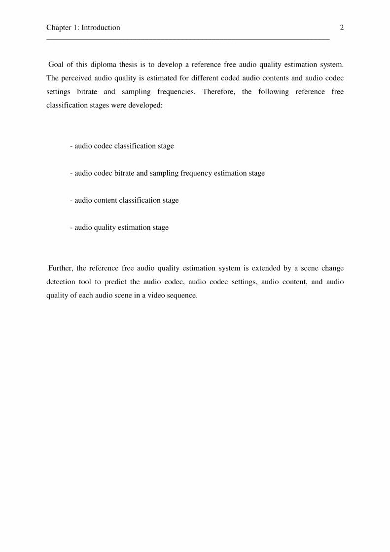
Goal of this diploma thesis is to develop a reference free audio quality estimation system.
The perceived audio quality is estimated for different coded audio contents and audio codec
settings bitrate and sampling frequencies. Therefore, the following reference free
classification stages were developed:
- audio codec classification stage
- audio codec bitrate and sampling frequency estimation stage
- audio content classification stage
- audio quality estimation stage
Further, the reference free audio quality estimation system is extended by a scene change
detection tool to predict the audio codec, audio codec settings, audio content, and audio
quality of each audio scene in a video sequence.

Chapter 2: Perceptual audio quality measurement and assessment methods ________________________________________________________________________
3
Chapter 2
Perceptual audio quality measurement
and assessment methods
The perceived audio quality of different coded audio contents, e.g., speech, music, or effect
sounds (fx), can be measured by subjective or objective audio quality assessment methods.
Objective perceptual audio quality measurement methods, based on mathematic algorithm,
are developed to simulate or substitute the situation of subjective perceptual audio quality
measurement methods (subjective MOS listener tests), in which test listeners scores the audio
quality of different coded audio files with different coded audio codec settings bitrate and
sampling frequency. The result of a subjective listener test is called the “mean opinion score”
(MOS), an integer value between 1 (bad) and 5 (excellent), which reflects the user opinion of
the perceived audio quality of a coded audio file. During a long time, subjective test
procedures were the only method of measuring the perceptual audio quality impression of
coded audio files. Subjective experiments require a huge number of subjects or test listeners
to achieve statistically relevant results, and so, they are very costly and time consuming.
Further, the great contrast between evaluation results and perceived audio quality leads to the
question, how to interpret the result. For perceptual audio quality measurement, subjective
listener tests are not optimal to estimate the perceived audio quality. Therefore, perceptual
models, based on mathematic algorithms, can be applied to generate model output variables or
parameters for objective audio quality metrics (“objective MOS” or “OMOS”) to predict the
perceived audio quality of coded audio content objective audio quality measurement systems).
The estimation results of audio quality metrics, consisting of those model output parameters,
can be compared with subjective MOS test results or directly with the values of a mean
opinion score scale.
In the research area of perceptual model processing, many detailed model output values, such
as frequency spectrum components, dynamically measured bandwidth, distortions, or
modulation will be generated and reported for making this technology universally applicable.
Chapter 2: Perceptual audio quality measurement and assessment methods ________________________________________________________________________
4
Those objective quality assessment methods stand in strong relation to the behaviour of
human perception and human judgement. To predict the perceived audio quality of a coded
audio file of a mobile audio service (audio streaming), it is necessary to find optimal relations
between parameter, which can be measured, (transmission errors, noise, distortion and losses
due to low bit-rate coding and packet transmission) and the human quality perception process.
Once, such a relation is found, audio, video, or audiovisual quality estimation metrics, based
on reference information or not, can be designed.
Until now, many different quality evaluation metrics for low bitrate applications have been
proposed [1-5]. The basic metrics for non-reference free perceptual audio quality estimation
are including “objective” criterions, such as objective difference grades or mean-square error
based criterions [6], and results from subjective listener tests to estimate the user perceived
audio quality. While in subjective quality assessment methods test persons rate the quality of
a service or the quality of coded multimedia content, objective quality measurement or
assessment methods try to predict those user perceptual quality impressions using mathematic
algorithm. Those objective measurement or assessment algorithms estimate the perceived
audio quality using reference information (reference based objective assessment methods) or
not (reference free objective assessment methods).
2.1 Objective perceptual audio quality measurement and assessment
methods
Objective audio quality assessment methods try to simulate cost- and time expensive
subjective audio quality measurement methods (subjective listener tests) by perceptual
measurement algorithms. The basic structure of objective perceptual audio quality
measurement systems can be divided into a perceptual model stage, a feature extraction stage,
and a cognitive model stage for the objective measurement, as described in more details in
section 2.1.1. Objective audio quality measurement algorithms or systems can be divided into
two main groups: reference free and reference based objective perceptual measurement
systems. Input of reference based perceptual measurement systems are the coded, degraded
audio file and its original, uncoded version as reference source. Such perceptual measurement
algorithm are always reference based, that means, that there is always a need for a reference
Chapter 2: Perceptual audio quality measurement and assessment methods ________________________________________________________________________
5
information to calculate the perceptual Measurement Output Variables (MOV’s), which are
further used as the parameter of audio quality estimation metrics. While the coefficients of
those parameter are always audio codec and audio content specific, it is possible to choose
automatically the audio codec and audio content specific parameter coefficients for each
audio codec and audio content by using an audio codec and audio content classification stage.
The development of an effective objective perceptual quality measurement or assessment
method for a specific type of telecommunication signal, such as audio or speech, is a
significant research problem. Several objective quality assessment methods have already been
developed in recent years and those methods may be applied directly on a perceptual model
output, which simulates the human auditory system and cognitive behaviour of human beings
[7-14]. Further, the output of a good objective quality measurement method should have a
high correlation with many different subjective experiments. The closeness of the fit between
the results of an audio quality estimation metric, consisting of objective quality measurement
model or system output parameters, and the results of subjective test listener scores can be
measured by calculating a correlation factor or coefficient (cf. section 5.6.1).
As described above, objective measurement methods try to simulate the human perception
and human cognition behaviour using psychoacoustic models, based on psychoacoustic
phenomens, as investigated, e.g., in [15], [16], [17]. The most advanced objective perceptual
quality assessment methods may be found in the areas of audio and speech, while for those
telecommunication signals psycho-acoustic effects, known from masking experiments, are
differing in a significant way. For wideband audio signals, the PEAQ (Perceptual Evaluation
of Audio Quality) method has been developed and recommended by the ITU-R Rec. Bs.
1387 [7]. PEAQ was developed originally as an automated method to evaluate the perceptual
quality of different wideband audio codecs. Such codecs are used to sample wideband audio
signals and compressing the bit rate requirements. By applying the PEAQ algorithm to the
individual packet streams within the network performance model (e.g., the packet-switched
mobile networks, such as 3GP), it is possible to obtain objective perceptual quality output
measurement indicators for the investigated audio stream or audio file, which is analyzed by
the model. For speech signals, several objective perceptual quality assessment methods have
been developed, e.g., PAMS (Perceptual Analysis Measurement System) [8], [9], PSQM
(Perceptual Speech Quality Measurement) [10], and PESQ (Perceptual Evaluation of Speech
Chapter 2: Perceptual audio quality measurement and assessment methods ________________________________________________________________________
6
Quality), recommended by the ITU standard P.862 [11], or PEAQ (Perceptual Evaluation of
Audio Quality) [7] as objective perceptual audio quality measurement systems for coded
audio content. All of those methods are using natural or artificial speech signals as input
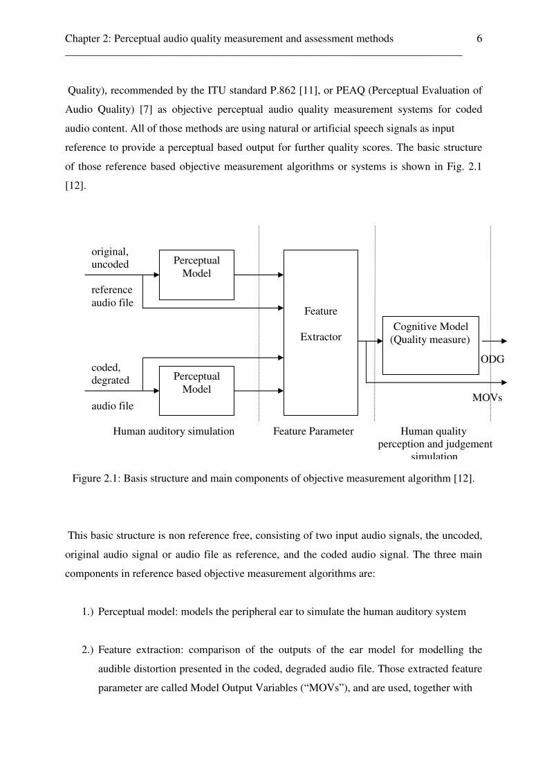
reference to provide a perceptual based output for further quality scores. The basic structure
of those reference based objective measurement algorithms or systems is shown in Fig. 2.1
[12].
Figure 2.1: Basis structure and main components of objective measurement algorithm [12].
This basic structure is non reference free, consisting of two input audio signals, the uncoded,
original audio signal or audio file as reference, and the coded audio signal. The three main
components in reference based objective measurement algorithms are:
1.) Perceptual model: models the peripheral ear to simulate the human auditory system
2.) Feature extraction: comparison of the outputs of the ear model for modelling the
audible distortion presented in the coded, degraded audio file. Those extracted feature
parameter are called Model Output Variables (“MOVs”), and are used, together with
Perceptual Model
original, uncoded reference audio file
Perceptual Model
coded, degrated audio file
Feature
Extractor Cognitive Model
(Quality measure)
Human auditory simulation Feature Parameter Human quality perception and judgement simulation
ODG MOVs
Chapter 2: Perceptual audio quality measurement and assessment methods ________________________________________________________________________
7
objective difference grade parameters (ODG), as the parameters in audio quality
estimation metrics.
3.) Deriving of a quality measure: consisting of a single number that indicates the
audibility of the distortions presents in the degraded audio file. This is done by
simulating the cognitive part of the human auditory system through further
processings of the model output variables MOVs.
Reference based perceptual models, as shown in Fig.2.1, use the undegraded, original audio
file and its coded version as input to calculate the audio codec and audio content specific
objective difference grade and model output variables. For predicting the audio quality of
different coded audio content automatically, the perceptual model should be extended with an
audio codec and audio content classification stage, to choose the codec and content specific
audio quality estimation metric and its coefficients. Examples for audio quality estimation
metrics for AMR and AAC coded speech content are given in equation (2.1) and (2.2), while
equation (2.3) gives an example for an audio quality estimation metric, suitable to predict the
perceived audio quality of AAC coded music content [1]:
AMR coded speech content: MOSA = - 6.996·AD² + 10.95·AD + 1.165 (2.1)
AAC coded speech content: MOSA = - 6.996·AD² + 10.95·AD + 0.370 (2.2)
AMR / AAC coded music content:
MOSA = - 3.1717 + 4.8809/IFD + 0.3562·A_ind + 0.0786·D_ind (2.3)
The metrics in equation (2.1) and (2.2) are based on the model output parameter auditory
distance AD from the Measuring Normalizing Block Technic for Objective Estimation of
Perceived Speech Quality [13], measuring dissimilarities between the original and degraded,
coded audio file.

Chapter 2: Perceptual audio quality measurement and assessment methods ________________________________________________________________________
8
The audio quality estimation metric parameters in equation (2.3) are based on the PESQ
(Perceptual Evaluation of Speech Quality) [11] model output parameters integrated frequency
distance IFD and the disturbance indicators A_ind and D_ind. Further, an example for a
perceptual speech quality metric for waveform codecs, CELP / hybrid codecs, and mobile
codecs / systems, based on model output variables symmetric and asymmetric disturbance
indicators (dSYM, dASYM) of the PESQ system, is presented in equation (2.4) [14]:
PESQMOS = 4.5 – 0.1 · dSYM – 0.0309 · dASYM (2.4)
The following section gives an overview of the international standardized perceptual audio
measurement methods mentioned in the section above:
1996 PSQM [10] : Perceptual Speech Quality Measure (intrusive), developed originally 1996
by KPN Research (Netherlands) and is now specified in the ITU-T
recommandation P.861 [10] PSQM was the first method based on
psychoacoustic measuring for predicting listening quality. While the use
of PSQM is essentially limited to assessing the quality of continous
speech signals, the intrusive Avanced Speech Quality Measure, developed
1998 also by KPN Research. PSQM+ is more suitable for packet speech
measurements. Further, PSQM+ improves the time- alignment of the
signals to be compared and also how silence periods and packet dropouts
are taken into account in evaluating subjective quality. In comparison
to PSQM+, it can be seen as a kind of basic “core” model with no gain-
or time-alignment for signal preprocessing.
1998 PEAQ [7] : Perceptual Evaluation of Audio Quality according to ITU-R
recommendation BS.1387, available as a basic and advanced model.
1999 MNB [13] : MNB is an Objective Estimation of Perceived Speech Quality using a
measuring normalizing block technique (MNB) and was developed by
Stephen Voran from NTIA as an appendix to recommendation P.861.
Since PSQM is limited to higher bit rate speech codecs operating over
error-free channels, it is not suitable for an objective measurement of the
Chapter 2: Perceptual audio quality measurement and assessment methods ________________________________________________________________________
9
perceived quality of highly compressed digital speech with bit errors or
frame erasures.
2000 PAMS [9] : Perceptual Analysis Measurement System, developed by the British
Telecom and was the first method to provide robust results for packet
voice signals
2001 PESQ [11] : Perceptual speech quality measure (intrusive), developed 2001 in a
collaboration between British Telecom and KPN Research and is the
new ITU-T Recommandation P.862 [11], [14]. It combines PSQM with
PAMS and is optimized for VoIP and hybrid end-to-end applications.
PESQ is the preferred method for measuring the perceptual quality of
packet speech signals.
Objective perceptual quality assessment methods are also being developed for video signals,
in particular by the Video Quality Experts Group (VQEG) [18], [19].
2.2 Subjective perceptual audio quality measurement and
assessment methods
Subjective mean opinion score (MOS) listener tests are necessary to get an impression, how
human beings are classifying the audio quality of coded audio content. With this information,
it is possible to design audio quality estimation metrics. In a subjective MOS test scenario,
different coded audio files are randomly played to the test listener, which classifies the
perceived audio quality impression of each coded audio file by using values of a MOS scale
in the range (1..5).
To get an impression of the perceived audio quality of different coded audio contents, in the
subjective MOS listener tests, coded audio test files were randomly numbered by hand at an i-
tune playlist in that way, that the audio content and the audio codec were different for each
MOS rating test. The playbacks of the audio files were done using i-tunes, and the audio files
Chapter 2: Perceptual audio quality measurement and assessment methods ________________________________________________________________________
10
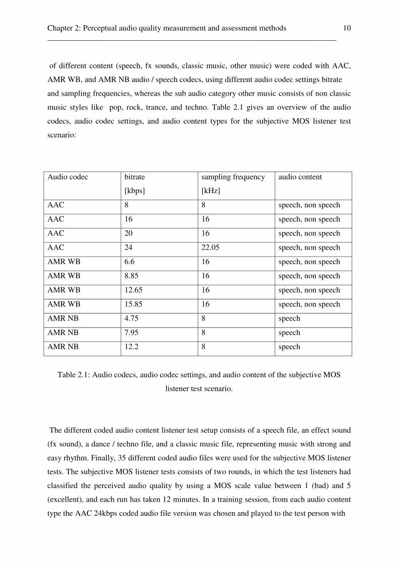
of different content (speech, fx sounds, classic music, other music) were coded with AAC,
AMR WB, and AMR NB audio / speech codecs, using different audio codec settings bitrate
and sampling frequencies, whereas the sub audio category other music consists of non classic
music styles like pop, rock, trance, and techno. Table 2.1 gives an overview of the audio
codecs, audio codec settings, and audio content types for the subjective MOS listener test
scenario:
Audio codec bitrate
[kbps]
sampling frequency
[kHz]
audio content
AAC 8 8 speech, non speech
AAC 16 16 speech, non speech
AAC 20 16 speech, non speech
AAC 24 22.05 speech, non speech
AMR WB 6.6 16 speech, non speech
AMR WB 8.85 16 speech, non speech
AMR WB 12.65 16 speech, non speech
AMR WB 15.85 16 speech, non speech
AMR NB 4.75 8 speech
AMR NB 7.95 8 speech
AMR NB 12.2 8 speech
Table 2.1: Audio codecs, audio codec settings, and audio content of the subjective MOS
listener test scenario.
The different coded audio content listener test setup consists of a speech file, an effect sound
(fx sound), a dance / techno file, and a classic music file, representing music with strong and
easy rhythm. Finally, 35 different coded audio files were used for the subjective MOS listener
tests. The subjective MOS listener tests consists of two rounds, in which the test listeners had
classified the perceived audio quality by using a MOS scale value between 1 (bad) and 5
(excellent), and each run has taken 12 minutes. In a training session, from each audio content
type the AAC 24kbps coded audio file version was chosen and played to the test person with
Chapter 2: Perceptual audio quality measurement and assessment methods ________________________________________________________________________
11
1,0
2,0
3,0
4,0
5,0
individual choosen playback volume level. AAC at 24kbps with 22.05kHz was chosen in the
training phase while this audio codec gives the best overall quality in the test scenario setup,
in comparison to the other used audio codecs and audio bitrates. So, the perceived audio
quality of AAC coded audio content at 24kbps can be seen as the upper bound of the
perceived audio quality / MOS scale (perceived audio quality reference value) and the
perceived audio quality of all other audio codecs were rated by the test listeners in relation to
this maximum perceived audio quality audio codec bound.
2.2.1 Subjective MOS listener test results for different coded audio
files
2.2.1.1 Test results for different coded speech files
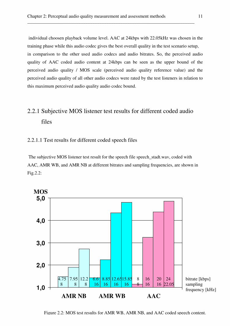
The subjective MOS listener test result for the speech file speech_stadt.wav, coded with
AAC, AMR WB, and AMR NB at different bitrates and sampling frequencies, are shown in
Fig.2.2:
MOS
4.75 7.95 12.2 6.6 8.85 12.6515.85 8 16 20 24 bitrate [kbps] 8 8 8 16 16 16 16 8 16 16 22.05 sampling frequency [kHz]
AMR NB AMR WB AAC
Figure 2.2: MOS test results for AMR WB, AMR NB, and AAC coded speech content.
Chapter 2: Perceptual audio quality measurement and assessment methods ________________________________________________________________________
12
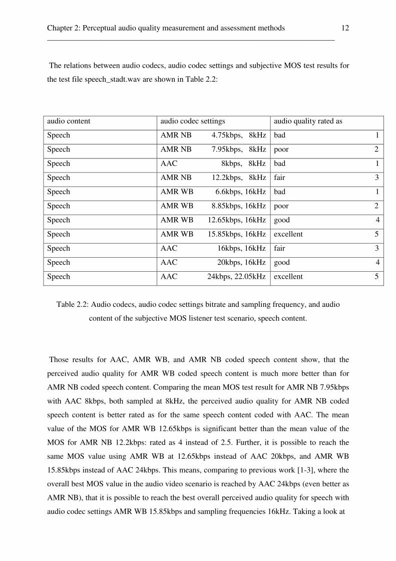
The relations between audio codecs, audio codec settings and subjective MOS test results for
the test file speech_stadt.wav are shown in Table 2.2:
audio content audio codec settings audio quality rated as
Speech AMR NB 4.75kbps, 8kHz bad 1
Speech AMR NB 7.95kbps, 8kHz poor 2
Speech AAC 8kbps, 8kHz bad 1
Speech AMR NB 12.2kbps, 8kHz fair 3
Speech AMR WB 6.6kbps, 16kHz bad 1
Speech AMR WB 8.85kbps, 16kHz poor 2
Speech AMR WB 12.65kbps, 16kHz good 4
Speech AMR WB 15.85kbps, 16kHz excellent 5
Speech AAC 16kbps, 16kHz fair 3
Speech AAC 20kbps, 16kHz good 4
Speech AAC 24kbps, 22.05kHz excellent 5
Table 2.2: Audio codecs, audio codec settings bitrate and sampling frequency, and audio
content of the subjective MOS listener test scenario, speech content.
Those results for AAC, AMR WB, and AMR NB coded speech content show, that the
perceived audio quality for AMR WB coded speech content is much more better than for
AMR NB coded speech content. Comparing the mean MOS test result for AMR NB 7.95kbps
with AAC 8kbps, both sampled at 8kHz, the perceived audio quality for AMR NB coded
speech content is better rated as for the same speech content coded with AAC. The mean
value of the MOS for AMR WB 12.65kbps is significant better than the mean value of the
MOS for AMR NB 12.2kbps: rated as 4 instead of 2.5. Further, it is possible to reach the
same MOS value using AMR WB at 12.65kbps instead of AAC 20kbps, and AMR WB
15.85kbps instead of AAC 24kbps. This means, comparing to previous work [1-3], where the
overall best MOS value in the audio video scenario is reached by AAC 24kbps (even better as
AMR NB), that it is possible to reach the best overall perceived audio quality for speech with
audio codec settings AMR WB 15.85kbps and sampling frequencies 16kHz. Taking a look at

Chapter 2: Perceptual audio quality measurement and assessment methods ________________________________________________________________________
13
the bad MOS test results for AMR WB and AMR NB for speech content, it seems not to be
clear, why AMR NB at 4.75kbps, 8kHz should be perceived better or similar to AMR WB at
6.6kbps, 16kHz.
Listening to the sound sample, it can be heard, that the AMR WB coded speech file sounds
“brighter” than the AMR NB coded version, caused by a sampling rate 16kHz for AMR WB
instead of the AMR NB sampling frequency 8kHz. It seems that the test listeners are more
sensitive about distortions in “brighter” audio files than for distortions in “smoother” audio
files. Maybe this can be compared with the effect of the human visual system in relation to the
field of television technic, where errors are represented by the color black in fact, that the
human eye is not so sensitive to black than white. Another reason why the speech codec AMR
WB at lower bitrates 6.6kbps and 8.85kbps is rated as bad, can be seen in the maximum
bound of the perceived audio quality of their AAC 24kbps versions and sampling frequency
22.05kHz. Further, in relation to the good MOS value of AMR WB at 12.65kbps and
15.85kbps, and in relation of AAC 20kbps and AAC 24kbps, the test persons perceived a
good threshold for what they rated as good or bad.
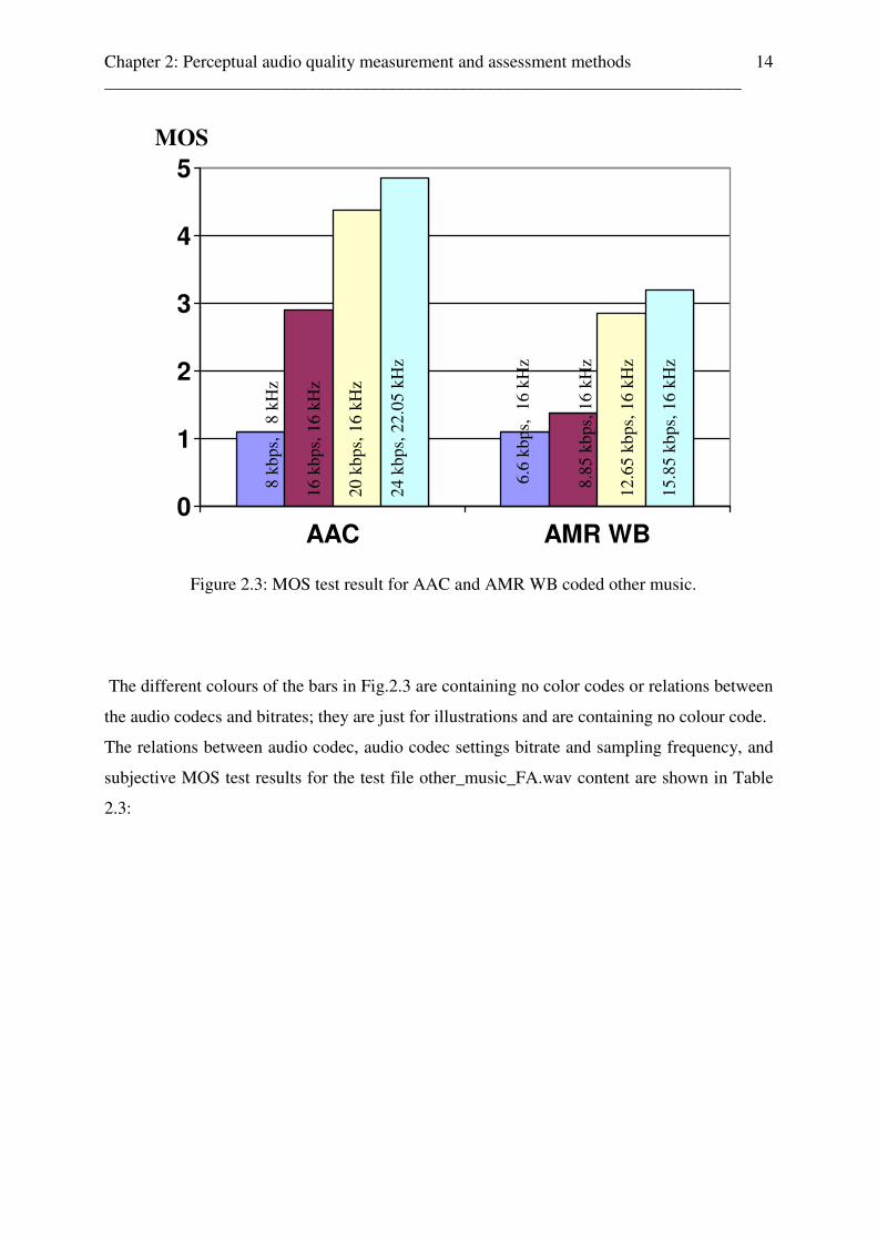
2.2.1.2 Test results for different coded other music
Test results from the subjective MOS listener test for the pop / techno test file
other_music_FA.wav, coded with AAC, AMR WB, AMR NB at different bitrates and
sampling frequencies, are shown in Fig.2.3:
Chapter 2: Perceptual audio quality measurement and assessment methods ________________________________________________________________________
14
The different colours of the bars in Fig.2.3 are containing no color codes or relations between
the audio codecs and bitrates; they are just for illustrations and are containing no colour code.
The relations between audio codec, audio codec settings bitrate and sampling frequency, and
subjective MOS test results for the test file other_music_FA.wav content are shown in Table
2.3:
0
1
2
3
4
5
AAC AMR WB
Figure 2.3: MOS test result for AAC and AMR WB coded other music.
8
kbps
, 8
kH
z 1
6 kb
ps, 1
6 kH
z 2
0 kb
ps, 1
6 kH
z 2
4 kb
ps, 2
2.05
kH
z
6.6
kbp
s, 1
6 kH
z
8.85
kbp
s, 1
6 kH
z 1
2.65
kbp
s, 1
6 kH
z 1
5.85
kbp
s, 1
6 kH
z
MOS

Chapter 2: Perceptual audio quality measurement and assessment methods ________________________________________________________________________
15
audio content audio codec settings audio quality rated as
other music AAC 8kbps, 8kHz bad 1
other music AMR WB 6.6kbps, 16kHz bad 1
other music AMR WB 8.85kbps, 16kHz bad 1
other music AAC 16kbps, 16kHz fair 3
other music AMR WB 12.65kbps, 16kHz fair 3
other music AMR WB 15.85kbps, 16kHz fair 3
other music AAC 20kbps, 16kHz good 4
other music AAC 24kbps, 22.05kHz excellent 5
Table 2.3: Audio codecs, audio codec settings bitrate and sampling frequency, and audio
content of the subjective MOS listener test scenario, other music.
Those test results for AAC and AMR WB coded other music show, that AMR WB is not a
suitable low bitrate audio codec for other music content in relation to high audio quality at
low bitrates, and the results for AAC coded music content are similar to previous works [1- 3].
The most suitable audio codec for other music in relation to the perceived audio quality is
AAC with codec settings 24kbps and sampling frequency 22.05kHz.
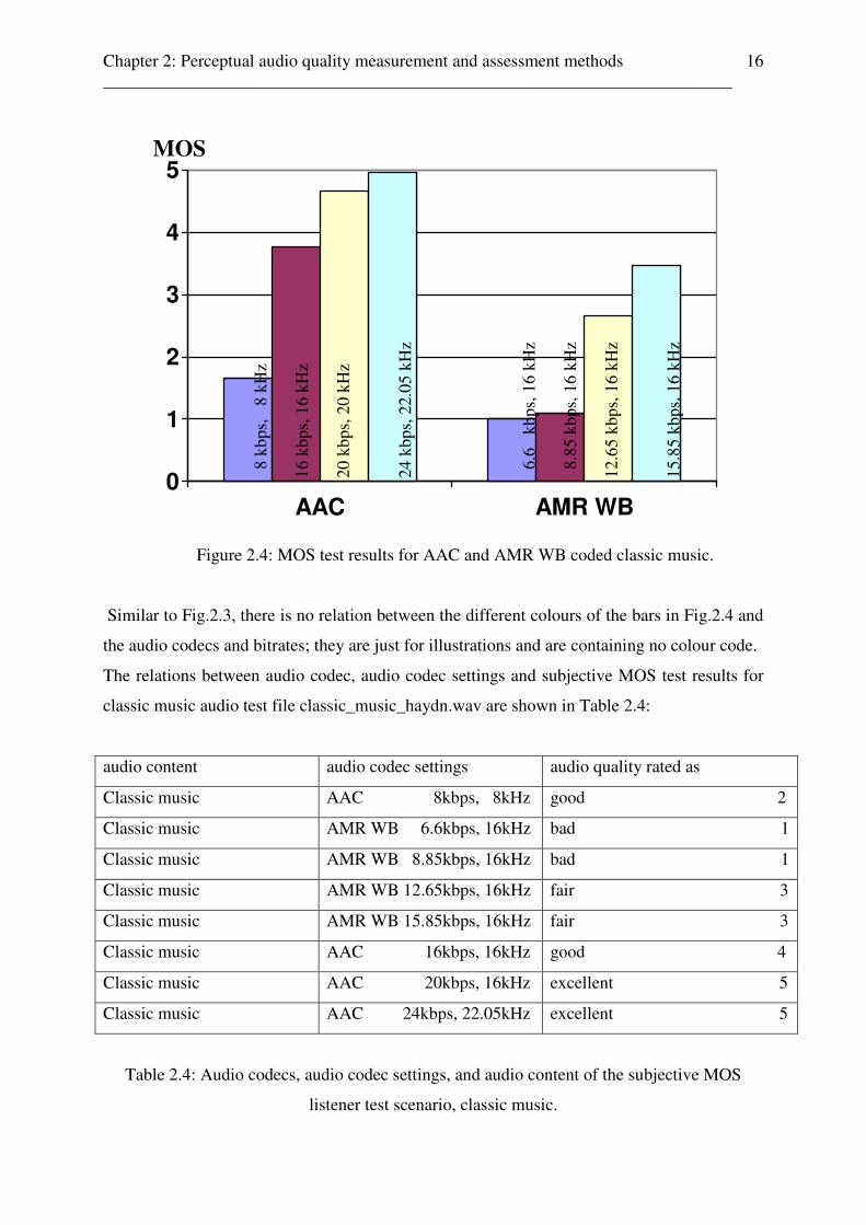
2.2.1.3 Test results for different coded classic music
Test results from the subjective MOS for the different coded classic music test file
classic_music_haydn.wav for different audio codecs and audio codec settings are shown in
Fig.2.4:
Chapter 2: Perceptual audio quality measurement and assessment methods ________________________________________________________________________
16
0
1
2
3
4
5
AAC AMR WB
Figure 2.4: MOS test results for AAC and AMR WB coded classic music.
Similar to Fig.2.3, there is no relation between the different colours of the bars in Fig.2.4 and
the audio codecs and bitrates; they are just for illustrations and are containing no colour code.
The relations between audio codec, audio codec settings and subjective MOS test results for
classic music audio test file classic_music_haydn.wav are shown in Table 2.4:
audio content audio codec settings audio quality rated as
Classic music AAC 8kbps, 8kHz good 2
Classic music AMR WB 6.6kbps, 16kHz bad 1
Classic music AMR WB 8.85kbps, 16kHz bad 1
Classic music AMR WB 12.65kbps, 16kHz fair 3
Classic music AMR WB 15.85kbps, 16kHz fair 3
Classic music AAC 16kbps, 16kHz good 4
Classic music AAC 20kbps, 16kHz excellent 5
Classic music AAC 24kbps, 22.05kHz excellent 5
Table 2.4: Audio codecs, audio codec settings, and audio content of the subjective MOS
listener test scenario, classic music.
MOS
8 k
bps,
8
kHz
16 k
bps,
16
kHz
20 k
bps,
20
kHz
24 k
bps,
22.
05 k
Hz
6.6
kb
ps, 1
6 kH
z 8
.85
kbps
, 16
kHz
12.6
5 kb
ps, 1
6 kH
z 15
.85
kbps
, 16
kHz
Chapter 2: Perceptual audio quality measurement and assessment methods ________________________________________________________________________
17
Similar to the results of AAC and AMR WB coded other music, AMR WB is not a suitable
low bitrate audio codec for classic music. But, comparing the bitrate MOS relation of AAC
16kbps coded classic music with those of AAC 16kbps coded other music, the test results
show, that there is a significant better MOS value for classic music coded AAC 16kbps (MOS
equal 4, good) comparing to other music (MOS equal 3, fair). As Table 2.4 shows, AAC
coded classic music with codec settings 20kbps and sampling frequency 16kHz is rated equal
AAC coded classic music with codec settings 24kbps and sampling frequency 22.05kHz. So,
it is possible to reach the same perceived audio quality for AAC codec classic music wih
lower bitrate and sampling frequency.
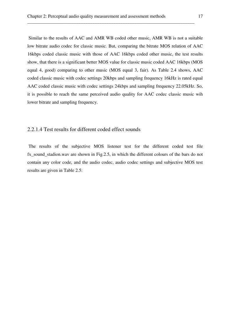
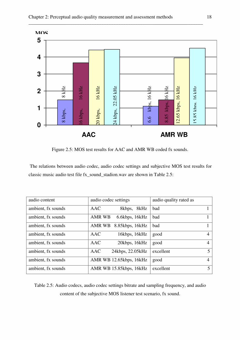
2.2.1.4 Test results for different coded effect sounds
The results of the subjective MOS listener test for the different coded test file
fx_sound_stadion.wav are shown in Fig.2.5, in which the different colours of the bars do not
contain any color code, and the audio codec, audio codec settings and subjective MOS test
results are given in Table 2.5:
Chapter 2: Perceptual audio quality measurement and assessment methods ________________________________________________________________________
18
Figure 2.5: MOS test results for AAC and AMR WB coded fx sounds.
The relations between audio codec, audio codec settings and subjective MOS test results for
classic music audio test file fx_sound_stadion.wav are shown in Table 2.5:
audio content audio codec settings audio quality rated as
ambient, fx sounds AAC 8kbps, 8kHz bad 1
ambient, fx sounds AMR WB 6.6kbps, 16kHz bad 1
ambient, fx sounds AMR WB 8.85kbps, 16kHz bad 1
ambient, fx sounds AAC 16kbps, 16kHz good 4
ambient, fx sounds AAC 20kbps, 16kHz good 4
ambient, fx sounds AAC 24kbps, 22.05kHz excellent 5
ambient, fx sounds AMR WB 12.65kbps, 16kHz good 4
ambient, fx sounds AMR WB 15.85kbps, 16kHz excellent 5
Table 2.5: Audio codecs, audio codec settings bitrate and sampling frequency, and audio
content of the subjective MOS listener test scenario, fx sound.
0
1
2
3
4
5
AAC AMR WB
8 k
bps,
8
kHz
16 k
bps,
16
kHz
20 k
bps,
16
kHz
24 k
bps,
22.
05 k
Hz
6.6
k
bps,
16
kHz
8.8
5 k
bps,
16
kHz
12.
65 k
bps,
16
kHz
15.
85 k
bps,
16
kHz
MOS
Chapter 2: Perceptual audio quality measurement and assessment methods ________________________________________________________________________
19
Those test results show, that the perceived audio quality of an ambient sound, coded with
AMR WB 15.85kbps, 16kHz are rated equal its AAC 24kbps version, sampled at 22.05kHz.
So, for the case of ambient fx sounds, it is possible to reach the same perceived audio quality
at lower bitrates and sampling frequencies. Further, the same ambient content coded with
AMR WB 12.65kbps, sampled at 16kHz is equal rated as its AAC 16kbps and AAC 20kbps
versions, both sampled at 16kHz.
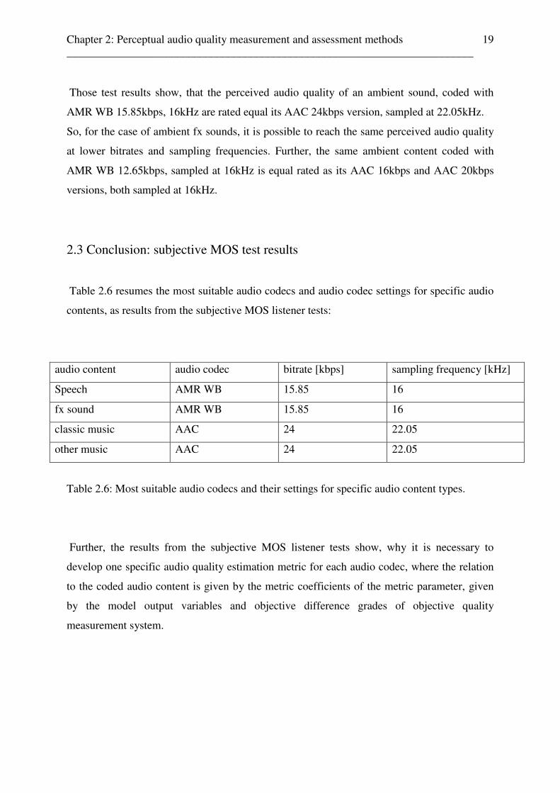
2.3 Conclusion: subjective MOS test results
Table 2.6 resumes the most suitable audio codecs and audio codec settings for specific audio
contents, as results from the subjective MOS listener tests:
audio content audio codec bitrate [kbps] sampling frequency [kHz]
Speech AMR WB 15.85 16
fx sound AMR WB 15.85 16
classic music AAC 24 22.05
other music AAC 24 22.05
Table 2.6: Most suitable audio codecs and their settings for specific audio content types.
Further, the results from the subjective MOS listener tests show, why it is necessary to
develop one specific audio quality estimation metric for each audio codec, where the relation
to the coded audio content is given by the metric coefficients of the metric parameter, given
by the model output variables and objective difference grades of objective quality
measurement system.
Chapter 3: Audio content classification ________________________________________________________________________
20
Chapter 3
Audio content classification
3.1. Overview
For audio quality estimation metrics and audiovisual quality estimation metrics to predict the
audiovisual quality for mobile streaming services it is necessary to develop an audio content
estimator to identify the audio content as speech or non speech, whereas non speech consists
of the audio sub categories effect sounds, classic music, other music. With such an estimator
it is possible to design automatic audiovisual metrics for audio and video quality estimation /
prediction. Such quality metrics consists of different coefficients for each kind of audio
content.
Related works have shown [1-5], that in case of audio it is necessary to evaluate two different
audio quality metrics, one for speech and one for non speech sequences, more exactly, one
audio quality metric for each kind of audio content (e.g., speech, non speech, different kind of
music styles, ambient / fx sounds). While non speech sequences, like music, sound effects,
noises, speech with background music or environmental sounds contain much more
information as speech, their main application can be found in cinema trailers, documentations,
advertisement or video clips (singer with background music). Based on this background, a
video stream or clip can be classified by its audio content (see chapter 6).
Existing works in the area of audio content classification presents different classification
methods, see [20 - 31] for more details. In [20], [22], [24] audio content classification is based
on signal characteristics in the time domain, in the frequency domain, in the time-frequency
domain and in the coefficient domain. All of them are using feature parameter extraction units
to classify sound signals by their individual characteristics. A good overview of parameters
which are usable for feature extraction is given in [20], [21], [22], [24], [25]. While in most of
the applications, only one parameter is not enough to design an optimal content classifier, the
Chapter 3: Audio content classification ________________________________________________________________________
21
combination of two or more parameter to a parameter mix (vector) in relation to the
application, as described, e.g., in [20], [21], [23] and [25], leads to acceptable classification
results. On the other hand, not all possible parameter which can be extracted from an audio
file are necessary for audio content classification, which is demonstrated in [21]. Further
parameter optimizations will lead to a much more lower complexity of the final audio quality
metrics. An example for the whole process of audio content classification by feature
extraction, feature vector design based on the mix of four chosen parameters and the
classification in subgroups is presented in [22]. For the final audio quality metric, an audio
content estimator for speech, music and speech with music is as important as an audio content
classification only for music genres and so, content classification methods, which are based
on the main difference in the nature of speech and non speech / music signals are necessary.
As mentioned in the previous chapter, there will be one audio quality metric designed for each
audio content type and so the number of different audio quality metrics corresponds to the
number of different chosen audio content subgenres. The periodicity in an audio content is
one of the most suitable characteristic for speech and music classification. This means, that in
all kind of music there can be found periodic patterns, given by the natural kind in the rhythm
[26], [31] of the audio content. Otherwise, such periodic patterns cannot be found in speech
content. The behaviour of speech signals is more random-like. Those characteristics can be
shown in the time domain and in the frequency domain:
- Time domain:
An indicator for periodic structures in a music signal can be found in the
zero-crossings of the signal, see [20], [22]. Here, the zero-crossings of a
music signal will appear nearly exactly after the same time-interval,
variating only in a very small range.
- Frequency domain:
In the frequency domain, the periodic pattern of music can be presented in
the spectral frequency density over the time, similar to [20], [22], and [25]. Such a mean
power pattern will show no periodic structure in the spectral frequency density for speech.
Chapter 3: Audio content classification ________________________________________________________________________
22
The first method is realized by analyzing the zero-crossing rate [20], which is the standard
deviation of the zero-crossings in all frames, divided by the frame length, while the second
method uses several subband energy ratios [24] to classify speech from music. So, two kinds
of estimation methods are investigated and compared: one in the time domain and one in the
frequency domain. Both of them are very fast and easy to implement in existing digital audio
signal processing programs. The estimators were proofed by the same test setup of audio files
to enable a comparison between them. This test setups contains different audio files from
different sources (CD or video) and have different lengths and contents. Some of them are
extracted from cinema trailers by hand for representing very short audio cuts to simulate the
further implementation of the estimators in video-cut depended audio content classification
systems. Further investigations of the estimators proof their suitability for different coded
audio contents. They should identify AAC or AMR WB / AMR NB coded speech with
background music, fx sound as music (non speech sequences), and AAC or AMR WB / AMR
NB coded speech as speech content.
3.2. Audio content classification based on zero-crossing rate estimator
3.2.1 General aspects
The first audio content classification method is realized by time domain characteristics of the
audio signal, so the original sound can be analysed without further transformations. This
method is similar as described in [20], [21], [22], [23]. According to [22], the audio file is
separated in frames of 150 sample values with 50% overlapping. Then, the number of zero-
crossings of each frame is calculated. A zero crossing occurs when the signal changes its
phase and can be detected when consecutive samples have different signs [22]. As described
in [24], the zero-crossing ratio is calculated by the number of time-domain zero-crossings
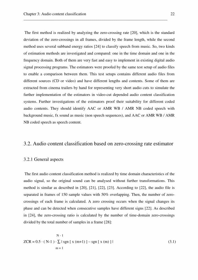
divided by the total number of samples in a frame [28]:
N - 1
ZCR = 0.5 · ( N-1 ) · ∑ | sgn [ x (m+1) ] – sgn [ x (m) ] | (3.1)
m = 1
Chapter 3: Audio content classification ________________________________________________________________________
23
where
sgn [·] … sign function
x(m) … discrete audio signal, m =1 … N.
N … frame length
0.5 … frame overlapping factor (50%)
While different audio sources have special characteristic in their zero-crossing rates, which is
illustrated in [20] and [22], this characteristics can be used as an estimator to separate
uncoded audio content classes speech, music, and all different styles of music and speech with
background music / noise. Speech with background music / noise can be further classified as
music.
Finally, to find a threshold value, the standard deviation of the zero crossing rates of all
frames, is a suitable indicator for classification. This threshold was found by analyzing the
audio test setup (see chapter 6.2.2) results at the value of 0.09 in case of uncoded speech or
non speech content.
3.2.2 Audio content classification for different audio content
As shown in related works [20], [22], and [29], the zero-crossing rates of different kinds of
audio contents follow typical characteristics for each content type. Typical speech
characteristics in relation to the zero crossing amplitudes are shown in Fig.3.7: high peaks of
the zero-crossing amplitudes over a relative low and stable line, which can be seen as a kind
of “baseline”, in relation to [20]. This results in a wide range (represented by the peaks and
troughs, caused by unvoiced and voiced components) and a large variance of the amplitudes.
The so called “baseline” is better demonstrated in case of music.
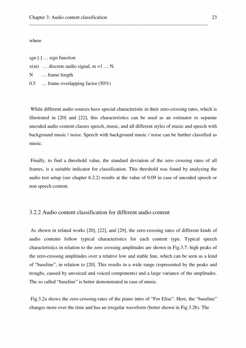
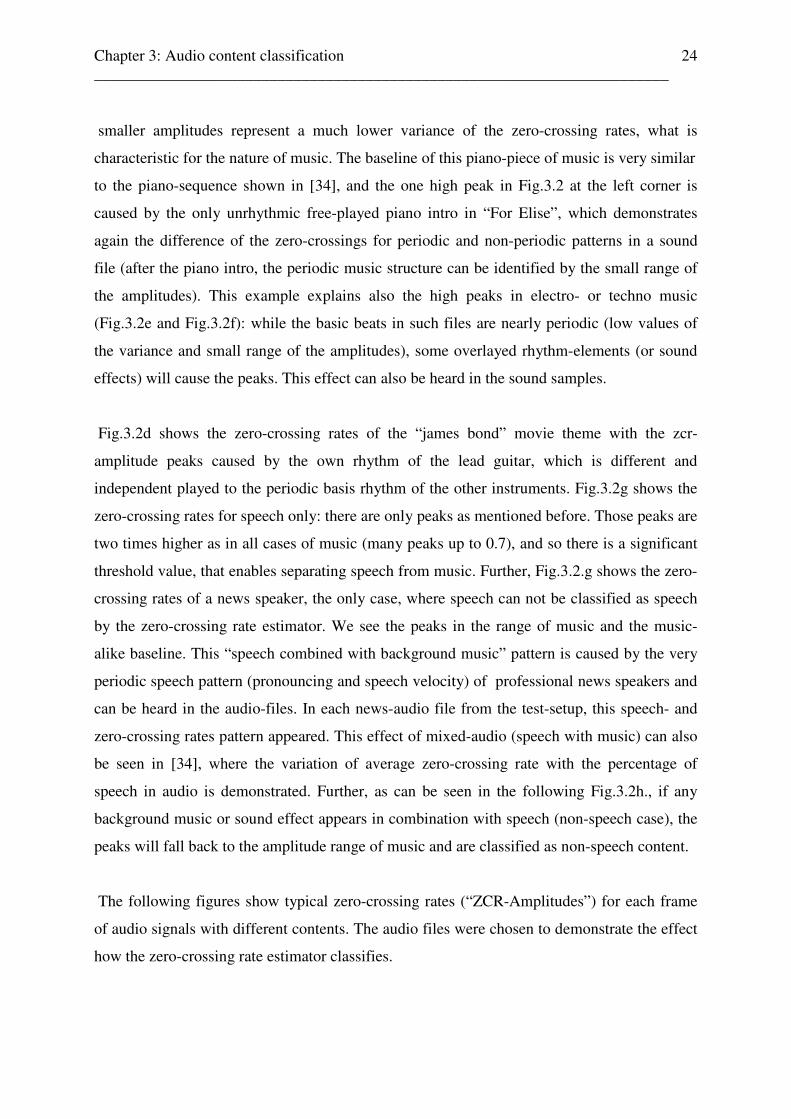
Fig.3.2a shows the zero-crossing-rates of the piano intro of “For Elise”. Here, the “baseline”
changes more over the time and has an irregular waveform (better shown in Fig.3.2b). The
Chapter 3: Audio content classification ________________________________________________________________________
24
smaller amplitudes represent a much lower variance of the zero-crossing rates, what is
characteristic for the nature of music. The baseline of this piano-piece of music is very similar
to the piano-sequence shown in [34], and the one high peak in Fig.3.2 at the left corner is
caused by the only unrhythmic free-played piano intro in “For Elise”, which demonstrates
again the difference of the zero-crossings for periodic and non-periodic patterns in a sound
file (after the piano intro, the periodic music structure can be identified by the small range of
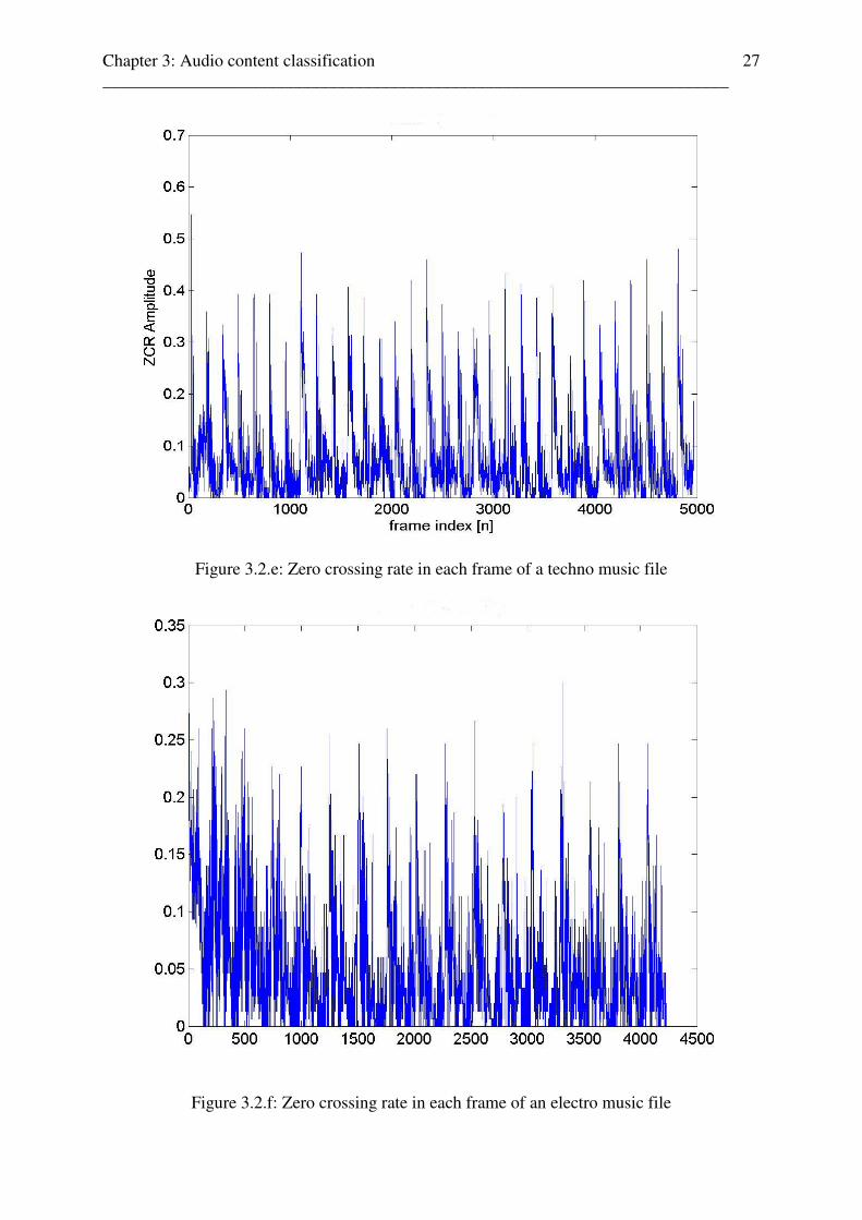
the amplitudes). This example explains also the high peaks in electro- or techno music
(Fig.3.2e and Fig.3.2f): while the basic beats in such files are nearly periodic (low values of
the variance and small range of the amplitudes), some overlayed rhythm-elements (or sound
effects) will cause the peaks. This effect can also be heard in the sound samples.
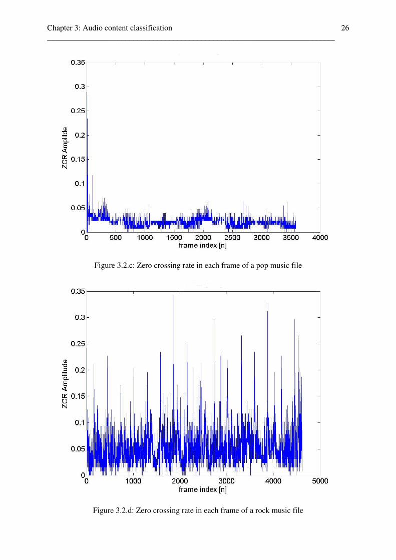
Fig.3.2d shows the zero-crossing rates of the “james bond” movie theme with the zcr-
amplitude peaks caused by the own rhythm of the lead guitar, which is different and
independent played to the periodic basis rhythm of the other instruments. Fig.3.2g shows the
zero-crossing rates for speech only: there are only peaks as mentioned before. Those peaks are
two times higher as in all cases of music (many peaks up to 0.7), and so there is a significant
threshold value, that enables separating speech from music. Further, Fig.3.2.g shows the zero-
crossing rates of a news speaker, the only case, where speech can not be classified as speech
by the zero-crossing rate estimator. We see the peaks in the range of music and the music-
alike baseline. This “speech combined with background music” pattern is caused by the very
periodic speech pattern (pronouncing and speech velocity) of professional news speakers and
can be heard in the audio-files. In each news-audio file from the test-setup, this speech- and
zero-crossing rates pattern appeared. This effect of mixed-audio (speech with music) can also
be seen in [34], where the variation of average zero-crossing rate with the percentage of
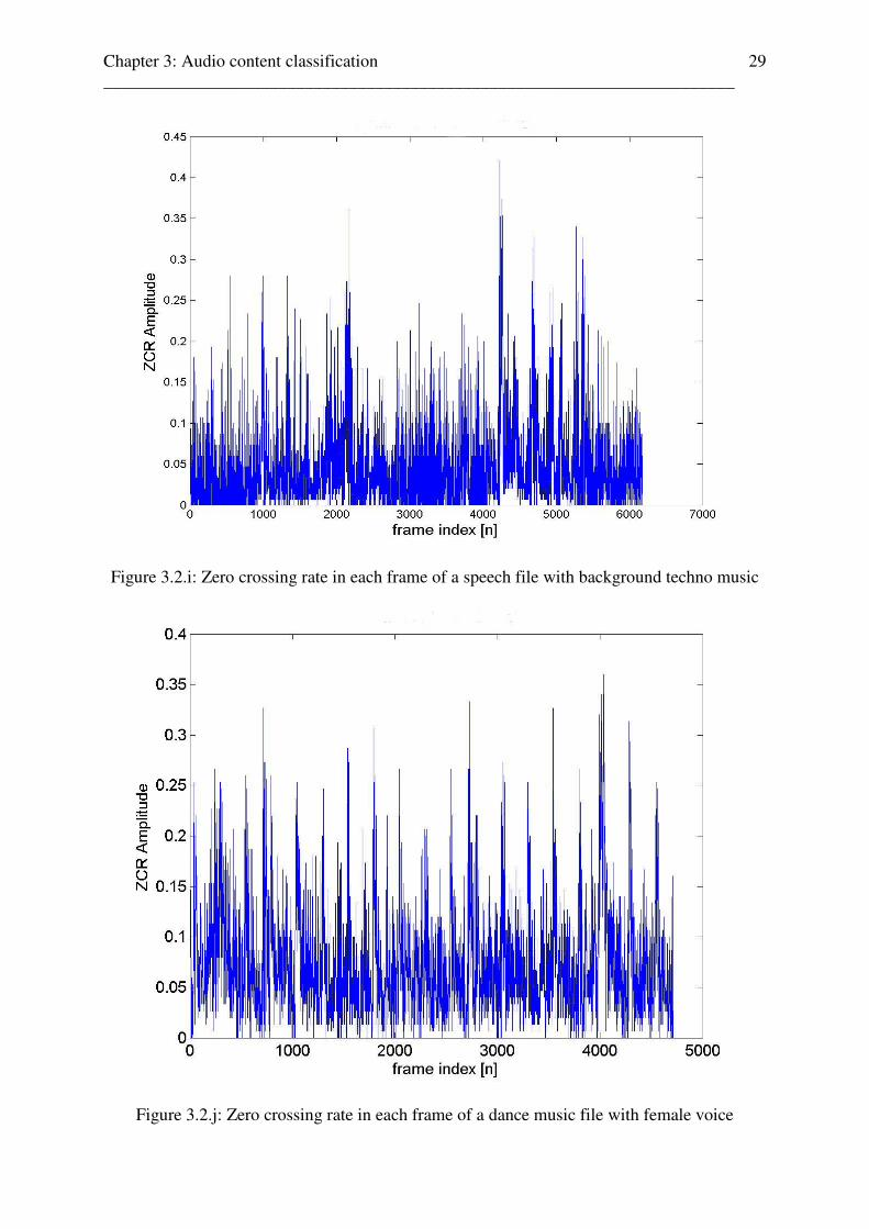
speech in audio is demonstrated. Further, as can be seen in the following Fig.3.2h., if any
background music or sound effect appears in combination with speech (non-speech case), the
peaks will fall back to the amplitude range of music and are classified as non-speech content.
The following figures show typical zero-crossing rates (“ZCR-Amplitudes”) for each frame
of audio signals with different contents. The audio files were chosen to demonstrate the effect
how the zero-crossing rate estimator classifies.
Chapter 3: Audio content classification ________________________________________________________________________
25
Figure 3.2.a: Zero crossing rate in each frame of a classic music file
Figure 3.2.b: Zero crossing rate in each frame of an orchestra music file
Chapter 3: Audio content classification ________________________________________________________________________
26
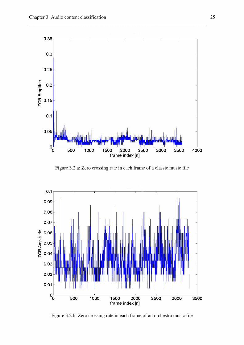
Figure 3.2.c: Zero crossing rate in each frame of a pop music file
Figure 3.2.d: Zero crossing rate in each frame of a rock music file
Chapter 3: Audio content classification ________________________________________________________________________
27
Figure 3.2.e: Zero crossing rate in each frame of a techno music file
Figure 3.2.f: Zero crossing rate in each frame of an electro music file

Chapter 3: Audio content classification ________________________________________________________________________
28
Figure 3.2.g: Zero crossing rate in each frame of a speech file
Figure 3.2.h: Zero crossing rate in each frame of a speech file with background sound fx
Chapter 3: Audio content classification ________________________________________________________________________
29
Figure 3.2.i: Zero crossing rate in each frame of a speech file with background techno music
Figure 3.2.j: Zero crossing rate in each frame of a dance music file with female voice
Chapter 3: Audio content classification ________________________________________________________________________
30
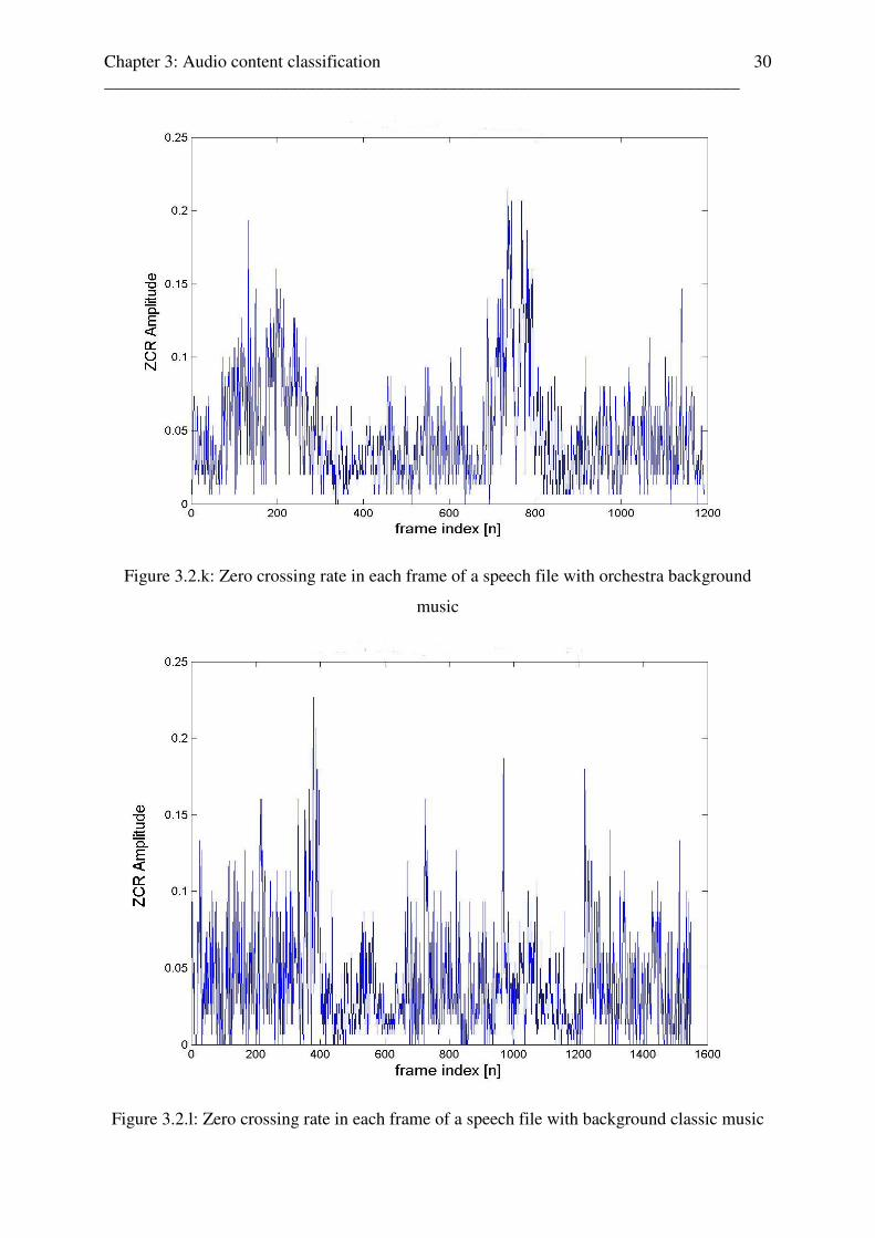
Figure 3.2.k: Zero crossing rate in each frame of a speech file with orchestra background
music
Figure 3.2.l: Zero crossing rate in each frame of a speech file with background classic music
Chapter 3: Audio content classification ________________________________________________________________________
31
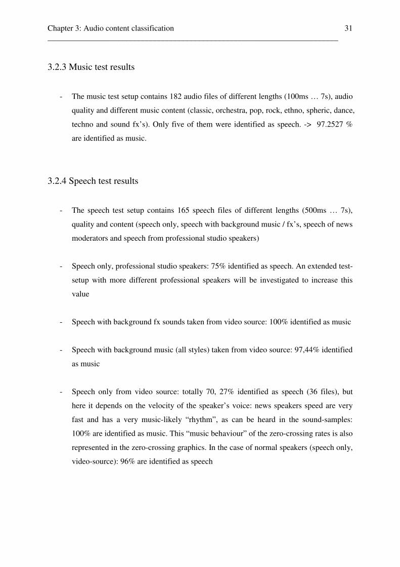
3.2.3 Music test results
- The music test setup contains 182 audio files of different lengths (100ms … 7s), audio
quality and different music content (classic, orchestra, pop, rock, ethno, spheric, dance,
techno and sound fx’s). Only five of them were identified as speech. -> 97.2527 %
are identified as music.
3.2.4 Speech test results
- The speech test setup contains 165 speech files of different lengths (500ms … 7s),
quality and content (speech only, speech with background music / fx’s, speech of news
moderators and speech from professional studio speakers)
- Speech only, professional studio speakers: 75% identified as speech. An extended test-
setup with more different professional speakers will be investigated to increase this
value
- Speech with background fx sounds taken from video source: 100% identified as music
- Speech with background music (all styles) taken from video source: 97,44% identified
as music
- Speech only from video source: totally 70, 27% identified as speech (36 files), but
here it depends on the velocity of the speaker’s voice: news speakers speed are very
fast and has a very music-likely “rhythm”, as can be heard in the sound-samples:
100% are identified as music. This “music behaviour” of the zero-crossing rates is also
represented in the zero-crossing graphics. In the case of normal speakers (speech only,
video-source): 96% are identified as speech
Chapter 3: Audio content classification ________________________________________________________________________
32
3.2.5 Conclusion: zero-crossing rate estimator
An estimator based on zero crossing rate identifies music and speech with background music
and effect sounds as music, which is ideal for analyzing cinema trailers, advertisements,
documentations, or, in the simplest case, the introduction of a music band by a moderator
(speech content -> music content -> music content with voice).
One great advantage of a zero-crossing estimator is the short identification time (correct
identifications for 500ms speech segments and 100ms music segments as shown in the tests).
Further, the calculation of the zero crossing rate is very simple and fast, it uses characteristics
of the original signal in the time domain (-> no further transformation).
In relation to audio codecs and audiovisual quality, an estimator based on zero crossing rate
enables to choose automatically the right coefficients for the parameter of the audio codec and
audio content specific audio quality metric parameter. For example, in case of AMR WB and
AMR NB coded speech content, audio codec and audio content specific coefficients for the
model audio quality output parameter auditory distance AD can be chosen from a table, or for
the case of music and music with speech coefficients, corresponding to AAC, coefficients for
the integrated frequency distance parameter IFD [1] and the disturbance indicators D_ind and
A_ind. The disadvantage of such an estimator is the identification of news-speakers (speech
only), while the voice of news speaker has a rhythmic similar to music. For coded audio
content, as described in chapter 5, the same method for audio content classification works also
for news speaker, based on a modified version of the coded audio file and a variation of the
threshold value.
Analyzing several news-clips, there can be said, that most of them follow the same structure:
music only as intro -> music with speech for the introduction -> then, most of the time only
speech, interrupted by sequences with speech and background noise / fx’s. Music with speech
sequences during a news-scenario are rare. Based on this average structure of news, further
test should prove, if such clips need audio content classification or if the information about
the video content [27] (news -> most time speech) is enough to classify them as speech, see
chapter 6. On the other hand, video content classification, based on audio scene characteristics,
is possible, as described in chapter 6. Another method is based on the usage of subband
Chapter 3: Audio content classification ________________________________________________________________________
33
energy estimation, in which the energy of a given frequency interval in the frequency domain
is calculated and compared to a threshold, dividing speech from non speech content. In the
case of news, subband energy estimation leads to better classification results than in the case
of non speech content. Test results of the zero crossing rate audio content classification are
given in appendix D.
3.3 Audio content classification based on subband energy estimator
3.3.1 General aspects
Content classification based on subband energy estimation uses sound characteristics in the
frequency domain, as presented, e.g., in [20], [22], [23], (2,5), while [24], [25] gives a good
overview of frequency-domain features. So the computation for this estimator is more
complex and not so easy as for the zero crossing rate estimator, if the estimator works alone
for itself. Otherwise, the implementation of this algorithm in a program which already works
with signal-framing, windowing, FFT and frequency splitting (normally most of programs
which deals with digital audio signal processing) is very easy and the algorithm will be
reduced only to calculate the subband energy ratio [24] comparing to the threshold level,
defined by the tests-results. Similar to the zero crossing estimator, an audio file is divided into
frames of 100 samples with 50% overlapping, windowed with a hamming window and each
frame is transformed to the frequency domain. The whole frequency spectra is divided into 4
subband intervals, similar to [24], given by the half of the sampling frequency (22050Hz). For
each frame the subband energy ratio is calculated. The final chosen subband intervals follows
the bounded intervals in [24], and are given by:
- Subband 1: (0-2756) Hz
- Subband 2: (2756-5512) Hz
- Subband 3: (5512-11025) Hz
- Subband 4: (11025-22050) Hz
Chapter 3: Audio content classification ________________________________________________________________________
34
Variations of the subband boundes were made (e.g., to concentrate them on the frequency
range of the speech formants), but they offered no better classification results or threshold
bounds, comparing the subband energy ratio of each subband to find a threshold for this ratio
to separate speech from music. For this, the subband energy ratio is calculated by dividing
each subband energy to the total energy of the spectra. As mentioned above, every single
frame of the audio signal is transformed to the frequency domain by Fourier and represents
further the distribution of the spectral energy over this audio frame. By this way, a
comparison of the spectral energy distribution of each audio frame is possible, which shows,
how the spectral energy will change in time during the whole audio file. In case of music,
periodic pattern will appear. A much more complexer method to find characteristic periodic
patterns in audio content is demonstrated in [26]. In this method, the envelope of an audio
signal, which can be seen as an amplitude-modulated wave, is extracted and the frequency
spectrum of this “modulation”-wave is calculated. The investigation of statistic information
(mean or standard deviation of the spectral energy distribution from frame to frame) to design
an estimator to detect periodic and rhythmic structures as the main difference of music and
speech was also done, but gave no further significant threshold values for classification.
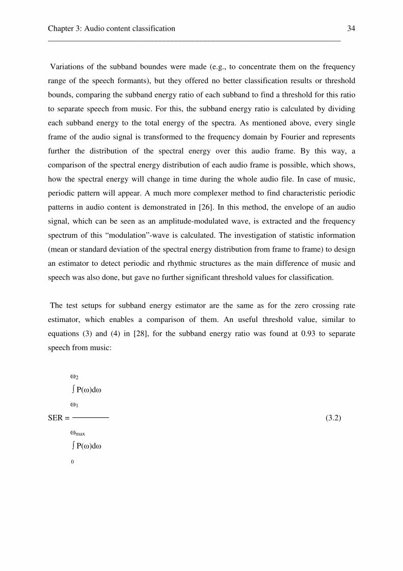
The test setups for subband energy estimator are the same as for the zero crossing rate
estimator, which enables a comparison of them. An useful threshold value, similar to
equations (3) and (4) in [28], for the subband energy ratio was found at 0.93 to separate
speech from music:
ω2
∫ P(ω)dω
ω1
SER = (3.2)
ωmax
∫ P(ω)dω
0
Chapter 3: Audio content classification ________________________________________________________________________
35
where
SER …… subband energy ratio
ω1, ω2 …. specific subband interval bounds
ωmax …… highest frequency of the spectrum
P(ω) …… Power at frequency ω, where P(ω) = |F(ω)|²
F(ω) …… FFT coefficients
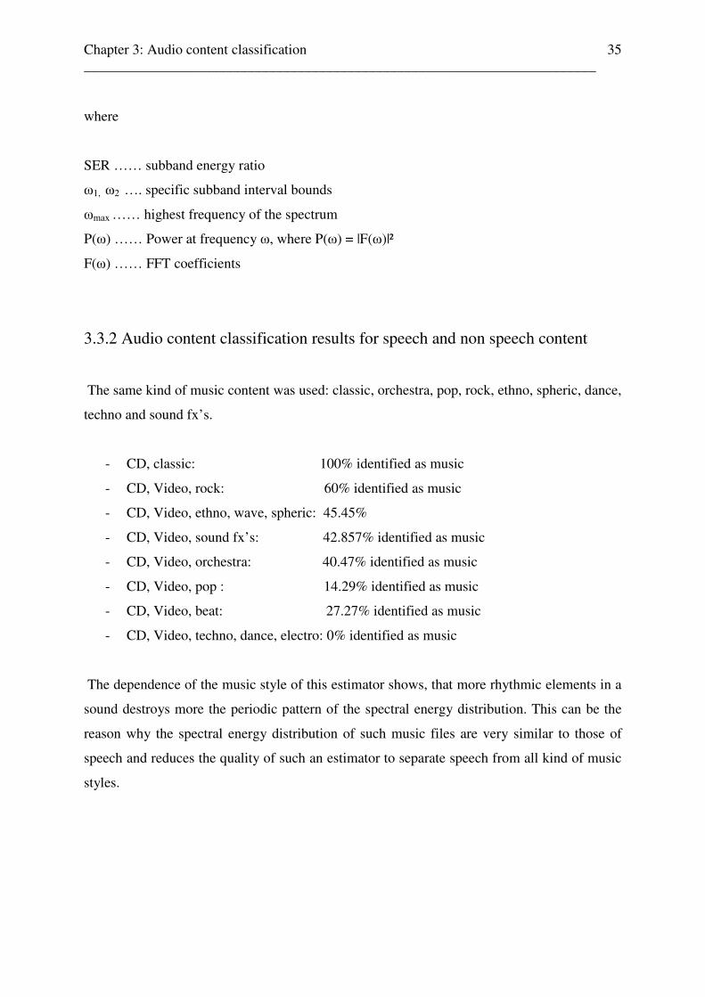
3.3.2 Audio content classification results for speech and non speech content
The same kind of music content was used: classic, orchestra, pop, rock, ethno, spheric, dance,
techno and sound fx’s.
- CD, classic: 100% identified as music
- CD, Video, rock: 60% identified as music
- CD, Video, ethno, wave, spheric: 45.45%
- CD, Video, sound fx’s: 42.857% identified as music
- CD, Video, orchestra: 40.47% identified as music
- CD, Video, pop : 14.29% identified as music
- CD, Video, beat: 27.27% identified as music
- CD, Video, techno, dance, electro: 0% identified as music
The dependence of the music style of this estimator shows, that more rhythmic elements in a
sound destroys more the periodic pattern of the spectral energy distribution. This can be the
reason why the spectral energy distribution of such music files are very similar to those of
speech and reduces the quality of such an estimator to separate speech from all kind of music
styles.

Chapter 3: Audio content classification ________________________________________________________________________
36
3.3.3 Speech test results
The speech test setup is the same as for the zero crossing estimator. Based on the spectral
energy distribution of speech as described before, the estimator will identify an audio content
as speech in every case of speech only, speech with background music or fx’s. Only 9% of all
165 test files of speech only, speech with background music and fx’s were identified as music.
For this reason such an estimator could be used alternatively for uncoded news. Detail results
for audio content classification, based on subband energy ratio in comparison to zero crossing
rate based audio content classification are given in appendix D .
3.3.4 Conclusion: subband energy ratio estimator
With subband energy estimation, it is not possible to identify speech with music as music
(which is relevant for audio codecs and audiovisual quality metrics) and the only audio sub
content category, which can be separated from speech, is classic music. Another disadvantage
of this estimator is the instability, that means, that, based on the algorithm, subband energy
ratio of some audio files could not have been calculated (3.48% of music and 3.363% of
speech test setup).
3.3.5 Final conclusion: audio content estimators
Finally it can be said, that for all kind of uncoded audio content (speech only, speech with
background music and fx’s, and songs) except for news-speakers the zero crossing estimator
is a suitable classifier for audio content classification: it identifies all different styles of music
and also the combinations speech and music (which is important for AAC codecs) as good as
all non-news-speakers. Further, the zero crossing rate estimator enables automatic content
classification for an audiovisual metric by analyzing very short audio file segments, and this
estimator is easy to implement. Subband energy ratio estimator will be suitable for news
speakers, but not for separating music from speech and so this estimator is not preferable for
the design of an automatic audiovisual metric. This estimator is easy to implement in most of
digital audio signal processing programs.
Chapter 3: Audio content classification ________________________________________________________________________
37
3.4 Audio content classification for video sequences
In relation to audiovisual quality for multimedia content it is necessary to estimate the audio
content in one or more video sequences. Therefore, the zero-crossing estimator will classify
the audio content as speech or non speech. The main difference to audio only content
classification is the changing of the content between several video cuts (video sequences).
The estimation time intervals for audio content classification here are much shorter in which
the audio content can be analyzed and the estimation classification result depends on every
single video sequence content.
3.4.1 Audio content classification based on video cut time points
To estimate the audio content in a video sequence it is necessary to find the start- and end
points of every video scene in a video file. By using a scene change detection tool, it is
possible to transform the frame number of the video cuts into time points in seconds to find
the equivalent scene change time points in the audio track to synchronize the multimedia
components audio and video. After that, there are three methods for the estimation time
interval length in each video sequence, depending on the video content:
- each single sequence will be analyzed during its whole length
- each single sequence will be analyzed during 30% and 50% of its length
- the shortest cut time difference or the average sequence length of all sequences
3.4.2 Test results: music videos
All of the music videos from the setup are classified for 100% as music (without lead in /
lead out effects). Appendix contains the table with the test results.
Chapter 3: Audio content classification ________________________________________________________________________
38
3.4.3 Test results: music documentary
Music documentaries enables the simplest case to investigate video-cut based audio content
estimation:
- First sequence: speech (introduction of the artist)
- Second sequence: music (song)
The test files “roy black” and “angel_end”, which follow this structure, were classified 100%
as music. Test files “angel_start” and “come_undone” were classified as 90% and 89% as
music. Those results based on the fact, that in this test files the music of music sequences
fades in and out into the speech sequences. Appendix E contains the table with the test results.
3.4.4 Test results: cinema trailers
The test-setup for cinema trailers consists of:
- Cinema trailers with non-speech content (music or speech with
background music in every scene) only, fast and slow scenes
- Cinema trailers with speech and non-speech content (music or speech with
background music in every scene), fast and slow scenes
For cinema trailers, lead in and lead out effects at the beginning and the end of the whole
trailer causes false classifications for the first and last video sequences and were not used in
the analyzation process.
The tests of audio content classification for weather and advertisements are done for coded
audio content in chapter 6. Appendix E contains the table with the test results.

Chapter 4: Reference based and reference free audio quality estimation ________________________________________________________________________
39
Chapter 4
Reference based and reference free audio quality
estimation
4.1 Reference based audio quality estimation for different coded audio contents
Previous works [1-5] and the results from the subjective MOS listener tests (cf. 2.2.2.) show,
that for mobile streaming services AMR WB / AMR NB are the most suitable audio codecs
for speech content and AAC for music content. Further, it is possible to reach the same
perceived audio quality for a coded speech content file using AMR WB with codec settings
15.85kbps, 16kHz instead of the advanced audio codec AAC, working at 24kbps with
sampling frequency 22.05kHz. Together with the characteristics of each audio codec, zero-
crossing rate estimation allows the identification of the content of an encoded audio file.
Further, in relation to audio quality metrics and perceptual models [1-11], it is possible to
design one automatic audio quality metric with different metric parameter coefficients for
each encoded content type and specific objective quality measurement system model output
parameter to estimate the audio quality of a coded audio file. Therefore, audio codec and
audio content classifications are necessary. Once, the audio codec and audio content are
estimated, the specific audio quality metric coefficients for the specific objective quality
measurement model output parameters can be chosen from a table [1-3]. While the coded
audio content can be classified by zero crossing rate estimation, the audio codecs can be
classified by their individual setting characteristics or, as for the case of AAC and AMR, by
comparing the different lengths of the original and encoded audio file (reference based audio
codec classification):
- AMR decreases the length of the coded signal: length(orig) - length(degr) > 0
- AAC increases the length of the coded signal: length(orig) - length(degr) < 0
Chapter 4: Reference based and reference free audio quality estimation ________________________________________________________________________
40
Based on the information about the audio content, determed by audio content classification,
audio codec, and original audio file as reference, one audio quality metric with different
coefficients for each audio codec and audio content can be designed (see chapter 2).
4.2 Reference free audio quality estimation for different coded audio contents
The disadvantage of reference based audio quality estimation methods in relation to
complexity and computation power of the quality assessment methods is the usage of original,
uncoded or coded reference files, consisting of different audio contents. While all of those
reference depended algorithms are finally based on the comparison between an original,
uncoded or coded, degraded audio file as reference information, a calculation of the perceived
audio quality without information about such reference files is not possible. Moreover, a
collection of reference files with typical content or codec characteristics stored for
comparison will increase calculation time and the complexity of the audio quality metrics and
systems. Such reference based audio quality classification systems are always limited by the
available reference file collection and their classification characteristics. All of those
disadvantages can be avoided by the development of reference-free audio quality estimation
metrics or systems. Furthermore, reference-free metric parameter, which are determed directly
from the frequency spectrum of an unknown coded audio file without the usage of objective
quality measurement model outputs or algorithms, will decreases the complexity of the whole
estimation / calculation / classification process. This reduction is possible, if all design
processes of perceptual audio quality models and metrics are based on the statistic results of
subjective listener tests (MOS scale values, see sub chapter 2.2.1). So, the reduction of an
audio quality metric, consisting of parameter extracted by objective quality measurement
systems and their coefficients, to a single audio quality equation, consisting of audio quality
parameter extracted from the degraded, coded audio file frequency spectrum without specific
reference information will lead to the ideal case of lowest “metric” complexity, computational
power and calculation time, mathematically formulated as AQ = aqpc * aqfp, where aqfp is
the extracted audio quality feature parameter, aqpc the audio quality parameter coefficient,
and AQ the resulting audio quality. For this case, the audio quality equation parameter
coefficient aqpc must stand in relation to the mean result of how listeners would classify the
perceived audio quality of test files consisting of the same audio characteristics. Once, one or
Chapter 4: Reference based and reference free audio quality estimation ________________________________________________________________________
41
more parameter coefficients are found, such a relation is possible by a simple mapping
function between the audio quality parameter coefficient aqpc and the mean of the subjective
MOS test results for a specific coded audio content type (speech or non speech content).
As Fig.2.1 shows, parameter extracted by objective quality measurement models are always
based on reference values or information about the original, uncoded file, e.g., in case of
PESQ, the auditory distance AD between the original and degraded audio file or the
integrated frequency distance IFD between the original and degraded audio file. In case of
reference free parameter extraction, the extracted parameter is deviated directly from the
frequency spectrum of the coded audio file without further reference information about the
original, uncoded file or audio codec settings. The results of the subjective MOS audio
listener tests show the influence of each single audio codec with its individual performance
settings bitrate and sampling frequency on the perceived audio quality of different coded
speech or non speech content. While in most of the reference based audio quality
classification systems the parameter for the audio quality metric are extracted by objective
quality measurement models, reference free audio quality equation parameters are extracted
directly from the coded audio file without reference information, and their coefficients are
determed directly by the results of subjective MOS tests. So, the quality of the classification
process is given by the quality of the MOS test setup (number of different coded audio
content, number of test listeners, ...) and its results. Once a MOS test session is done, an
individual reference free audio quality feature parameter coefficient for that specific test setup
can be extracted by using specific time- or frequency domain algorithms, representing all
characteristics which influences the audio quality of each single test file.
Table 4.1 resumes the different coded audio test files from the subjective MOS listener tests
and their individual settings, representing the main characteristics of the chosen MOS test
setup to find a suitable audio quality classification metric for different coded audio content:
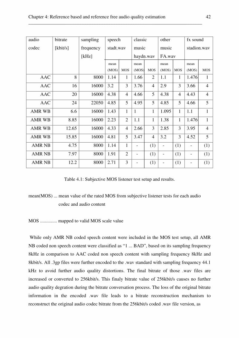
Chapter 4: Reference based and reference free audio quality estimation ________________________________________________________________________
42
audio
codec
bitrate
[kbit/s]
sampling
frequency
[kHz]
speech
stadt.wav
mean
(MOS) MOS
classic
music
haydn.wav
mean
(MOS) MOS
other
music
FA.wav
mean
(MOS) MOS
fx sound
stadion.wav
mean
(MOS) MOS
AAC 8 8000 1.14 1 1.66 2 1.1 1 1.476 1
AAC 16 16000 3.2 3 3.76 4 2.9 3 3.66 4
AAC 20 16000 4.38 4 4.66 5 4.38 4 4.43 4
AAC 24 22050 4.85 5 4.95 5 4.85 5 4.66 5
AMR WB 6.6 16000 1.43 1 1 1 1.095 1 1.1 1
AMR WB 8.85 16000 2.23 2 1.1 1 1.38 1 1.476 1
AMR WB 12.65 16000 4.33 4 2.66 3 2.85 3 3.95 4
AMR WB 15.85 16000 4.81 5 3.47 4 3.2 3 4.52 5
AMR NB 4.75 8000 1.14 1 - (1) - (1) - (1)
AMR NB 7.97 8000 1.91 2 - (1) - (1) - (1)
AMR NB 12.2 8000 2.71 3 - (1) - (1) - (1)
Table 4.1: Subjective MOS listener test setup and results.
mean(MOS) ... mean value of the rated MOS from subjective listener tests for each audio
codec and audio content
MOS .............. mapped to valid MOS scale value
While only AMR NB coded speech content were included in the MOS test setup, all AMR
NB coded non speech content were classified as “1 ... BAD”, based on its sampling frequency
8kHz in comparison to AAC coded non speech content with sampling frequency 8kHz and
8kbit/s. All .3gp files were further encoded to the .wav standard with sampling frequency 44.1
kHz to avoid further audio quality distortions. The final bitrate of those .wav files are
increased or converted to 256kbit/s. This finaly bitrate value of 256kbit/s causes no further
audio quality degration during the bitrate conversation process. The loss of the original bitrate
information in the encoded .wav file leads to a bitrate reconstruction mechanism to
reconstruct the original audio codec bitrate from the 256kbit/s coded .wav file version, as

Chapter 4: Reference based and reference free audio quality estimation ________________________________________________________________________
43
described in sub chapter 5.2.3. This bitrate reconstruction mechanism is essential for the
automatic reference free audio quality classification in that way, that the individual chosen
bitrate has one of the strongest influence on the perceived audio quality, more than the
sampling frequency, as shown in Table 4.1. For example, the perceived audio quality of AAC
coded speech content with 20kbit/s is better rated than the quality of AAC coded speech
content with 16kbit/s, using the same sampling frequency of 16kHz.
Such a reference free audio quality classification design, based on a MOS test setup with
individual chosen audio content, audio codecs, different bitrates and sampling frequencies is
flexible for all other kind of other individual chosen MOS test setups, consisting of MOS test
setup characteristics audio codecs, bitrates, sampling frequencies and content types. That
means, that this reference free design method or strategy can be extended, focused or applied
on every other individual chosen test setup (universal reference free design method). There is
no difference in the design strategy, if the MOS test setup consists of other individual chosen
audio codecs, bitrates, sampling frequencies or audio content, while the design method is
based on the information extracted from the specific chosen MOS test setup and on no other
kind of other reference information.
Chapter 5: Reference free audio quality estimation system ________________________________________________________________________
44
Chapter 5
Reference free audio quality estimation system
5.1 Overview of a reference free audio quality estimation system
In reference free audio quality estimation systems, the audio quality of a coded audio file is
predicted by the following units:
- audio codec classification stage:
- audio codec classification stage to identify the unknown audio codec of the audio file
- audio codec bitrate recovery and sampling frequency classification stage
- audio content classification stage for coded audio content
- audio quality parameter feature extraction stage for different kind of coded audio
content and audio quality parameter coefficient prediction
- audio quality parameter coefficient to MOS scale value mapping stage
Each of those stages extracts specific feature parameter from the coded audio file for further
classification processes, based on threshold comparison, to enable reference free automatic
audio quality estimation metrics. For the case of reference free audio quality classification,
those classification processes are also necessary for mapping the audio quality parameter
coefficient c to its corresponding MOSApred value. In the first two steps of such an audio
quality classification system, the unknown audio codec, bitrate and sampling frequency are
identified within the audio codec characteristic classification unit, before the audio content
can be classified. After that, an audio quality parameter is extracted by the feature extraction
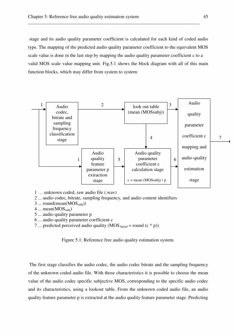
Chapter 5: Reference free audio quality estimation system ________________________________________________________________________
45
stage and its audio quality parameter coefficient is calculated for each kind of coded audio
type. The mapping of the predicted audio quality parameter coefficient to the equivalent MOS
scale value is done in the last step by mapping the audio quality parameter coefficient c to a
valid MOS scale value mapping unit. Fig.5.1 shows the block diagram with all of this main
function blocks, which may differ from system to system:
Figure 5.1: Reference free audio quality estimation system.
The first stage classifies the audio codec, the audio codec bitrate and the sampling frequency
of the unknown coded audio file. With those characteristics it is possible to choose the mean
value of the audio codec specific subjective MOS, corresponding to the specific audio codec
and its characteristics, using a lookout table. From the unknown coded audio file, an audio
quality feature parameter p is extracted at the audio quality feature parameter stage. Predicting
Audio codec,
bitrate and sampling frequency
classification stage
Audio quality feature
parameter p extraction
stage
Audio quality parameter
coefficient c calculation stage
c = mean (MOSsubj) / p
look out table (mean (MOSsubj))
stage
Audio
quality
parameter
coefficient c
mapping and
audio quality
estimation
stage
1 2 3 4 7 1 5 6 1 … unknown coded, raw audio file (.wav) 2 ... audio codec, bitrate, sampling frequency, and audio content identifiers 3 ... round(mean(MOSsubj)) 4 ... mean(MOSsubj) 5 ... audio quality parameter p 6 ... audio quality parameter coefficient c 7 ... predicted perceived audio quality (MOSApred = round (c * p))

Chapter 5: Reference free audio quality estimation system ________________________________________________________________________
46
the MOSA using a linear equation, an equation coefficient c is calculated as the ratio of the
chosen mean value of the subjective MOS and the audio quality feature parameter p.
Finally, this audio quality parameter coefficient c is mapped to a valid integer value in the
specific, audio codec characteristic range at the audio quality estimation stage. The correlation
between the rounded version of the subjective MOS mean value and the so predicted
MOSApred can be calculated by the Pearson linear correlation factor or by the characteristics of
a correlation vector. Fig.5.2 shows the same audio quality estimation system in a more
detailed version, while all function blocks from Fig. 5.1 are described in the following
chapters:
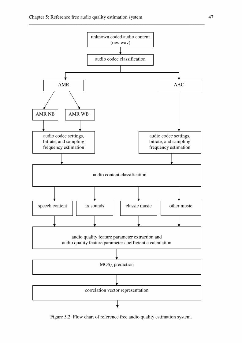
Chapter 5: Reference free audio quality estimation system ________________________________________________________________________
47
Figure 5.2: Flow chart of reference free audio quality estimation system.
unknown coded audio content (raw.wav)
audio codec classification
AMR AAC
AMR NB AMR WB
audio codec settings, bitrate, and sampling frequency estimation
audio codec settings, bitrate, and sampling frequency estimation
audio content classification
speech content fx sounds classic music other music
audio quality feature parameter extraction and
audio quality feature parameter coefficient c calculation
MOSA prediction
correlation vector representation
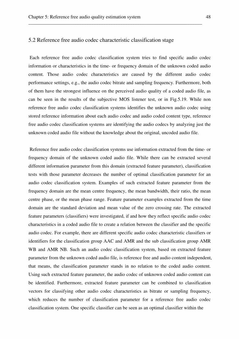
Chapter 5: Reference free audio quality estimation system ________________________________________________________________________
48
5.2 Reference free audio codec characteristic classification stage
Each reference free audio codec classification system tries to find specific audio codec
information or characteristics in the time- or frequency domain of the unknown coded audio
content. Those audio codec characteristics are caused by the different audio codec
performance settings, e.g., the audio codec bitrate and sampling frequency. Furthermore, both
of them have the strongest influence on the perceived audio quality of a coded audio file, as
can be seen in the results of the subjective MOS listener test, or in Fig.5.19. While non
reference free audio codec classification systems identifies the unknown audio codec using
stored reference information about each audio codec and audio coded content type, reference
free audio codec classification systems are identifying the audio codecs by analyzing just the
unknown coded audio file without the knowledge about the original, uncoded audio file.
Reference free audio codec classification systems use information extracted from the time- or
frequency domain of the unknown coded audio file. While there can be extracted several
different information parameter from this domain (extracted feature parameter), classification
tests with those parameter decreases the number of optimal classification parameter for an
audio codec classification system. Examples of such extracted feature parameter from the
frequency domain are the mean centre frequency, the mean bandwidth, their ratio, the mean
centre phase, or the mean phase range. Feature parameter examples extracted from the time
domain are the standard deviation and mean value of the zero crossing rate. The extracted
feature parameters (classifiers) were investigated, if and how they reflect specific audio codec
characteristics in a coded audio file to create a relation between the classifier and the specific
audio codec. For example, there are different specific audio codec characteristic classifiers or
identifiers for the classification group AAC and AMR and the sub classification group AMR
WB and AMR NB. Such an audio codec classification system, based on extracted feature
parameter from the unknown coded audio file, is reference free and audio content independent,
that means, the classification parameter stands in no relation to the coded audio content.
Using such extracted feature parameter, the audio codec of unknown coded audio content can
be identified. Furthermore, extracted feature parameter can be combined to classification
vectors for classifying other audio codec characteristics as bitrate or sampling frequency,
which reduces the number of classification parameter for a reference free audio codec
classification system. One specific classifier can be seen as an optimal classifier within the
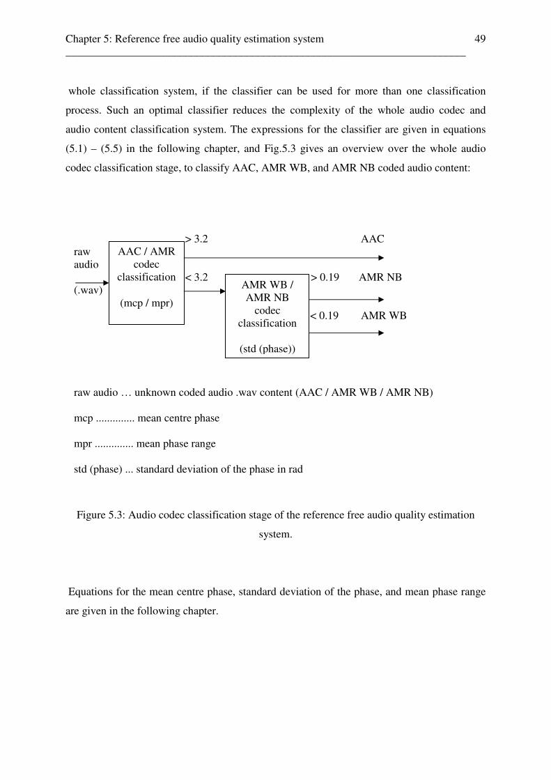
Chapter 5: Reference free audio quality estimation system ________________________________________________________________________
49
whole classification system, if the classifier can be used for more than one classification
process. Such an optimal classifier reduces the complexity of the whole audio codec and
audio content classification system. The expressions for the classifier are given in equations
(5.1) – (5.5) in the following chapter, and Fig.5.3 gives an overview over the whole audio
codec classification stage, to classify AAC, AMR WB, and AMR NB coded audio content:
Figure 5.3: Audio codec classification stage of the reference free audio quality estimation
system.
Equations for the mean centre phase, standard deviation of the phase, and mean phase range
are given in the following chapter.
AAC / AMR codec
classification
(mcp / mpr)
AMR WB / AMR NB
codec classification
(std (phase))
> 3.2 AAC raw audio < 3.2 > 0.19 AMR NB (.wav) < 0.19 AMR WB raw audio … unknown coded audio .wav content (AAC / AMR WB / AMR NB) mcp .............. mean centre phase mpr .............. mean phase range std (phase) ... standard deviation of the phase in rad
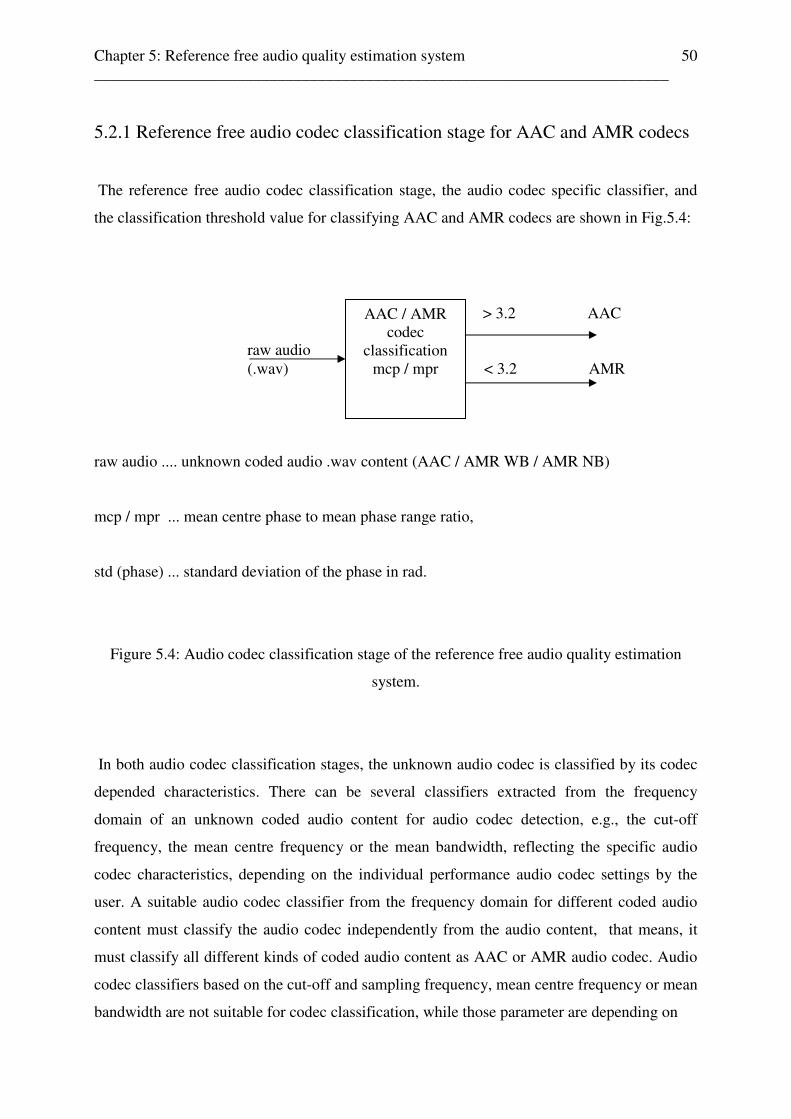
Chapter 5: Reference free audio quality estimation system ________________________________________________________________________
50
5.2.1 Reference free audio codec classification stage for AAC and AMR codecs
The reference free audio codec classification stage, the audio codec specific classifier, and
the classification threshold value for classifying AAC and AMR codecs are shown in Fig.5.4:
raw audio .... unknown coded audio .wav content (AAC / AMR WB / AMR NB)
mcp / mpr ... mean centre phase to mean phase range ratio,
std (phase) ... standard deviation of the phase in rad.
Figure 5.4: Audio codec classification stage of the reference free audio quality estimation
system.
In both audio codec classification stages, the unknown audio codec is classified by its codec
depended characteristics. There can be several classifiers extracted from the frequency
domain of an unknown coded audio content for audio codec detection, e.g., the cut-off
frequency, the mean centre frequency or the mean bandwidth, reflecting the specific audio
codec characteristics, depending on the individual performance audio codec settings by the
user. A suitable audio codec classifier from the frequency domain for different coded audio
content must classify the audio codec independently from the audio content, that means, it
must classify all different kinds of coded audio content as AAC or AMR audio codec. Audio
codec classifiers based on the cut-off and sampling frequency, mean centre frequency or mean
bandwidth are not suitable for codec classification, while those parameter are depending on
AAC / AMR codec
classification mcp / mpr
> 3.2 AAC raw audio (.wav) < 3.2 AMR
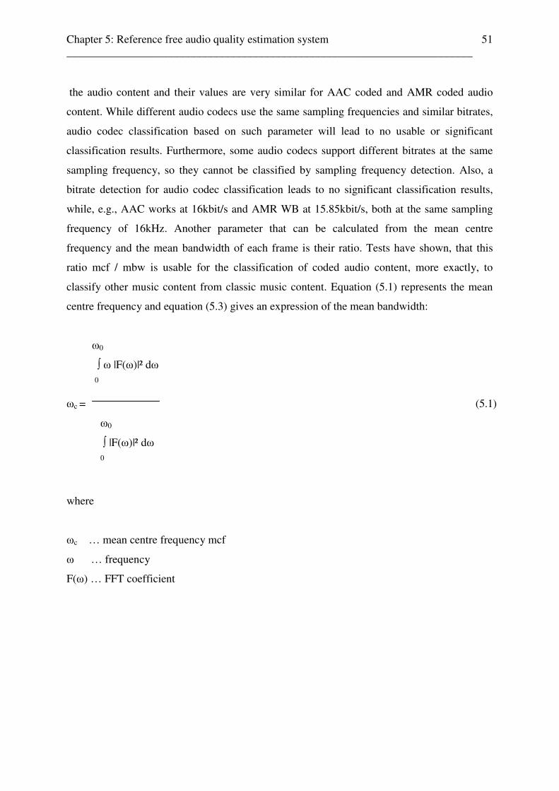
Chapter 5: Reference free audio quality estimation system ________________________________________________________________________
51
the audio content and their values are very similar for AAC coded and AMR coded audio
content. While different audio codecs use the same sampling frequencies and similar bitrates,
audio codec classification based on such parameter will lead to no usable or significant
classification results. Furthermore, some audio codecs support different bitrates at the same
sampling frequency, so they cannot be classified by sampling frequency detection. Also, a
bitrate detection for audio codec classification leads to no significant classification results,
while, e.g., AAC works at 16kbit/s and AMR WB at 15.85kbit/s, both at the same sampling
frequency of 16kHz. Another parameter that can be calculated from the mean centre
frequency and the mean bandwidth of each frame is their ratio. Tests have shown, that this
ratio mcf / mbw is usable for the classification of coded audio content, more exactly, to
classify other music content from classic music content. Equation (5.1) represents the mean
centre frequency and equation (5.3) gives an expression of the mean bandwidth:
ω0
∫ ω |F(ω)|² dω
0
ωc = (5.1)
ω0
∫ |F(ω)|² dω
0
where
ωc … mean centre frequency mcf
ω … frequency
F(ω) … FFT coefficient

Chapter 5: Reference free audio quality estimation system ________________________________________________________________________
52
ω 0
∫ (ω - ωc)² |F(ω)|² dω
0
B² = (5.2)
ω0
∫ |F(ω)|² dω
0
B = √B (5.3)
where
B … mean bandwidth mbw
ωc … mean centre frequency
ω … frequency
F(ω) … FFT coefficient
Further investigations have shown, that the mean ratio of the mean value and the mean range
of the phase of each audio signal frame, similar calculated as the mean centre frequency and
the mean bandwidth over all audio frames of an audio file, gives a significant classifier to
separate AAC coded audio content from AMR coded audio content in a content independent
way. The expressions for the mean centre phase and the mean phase range are given in
expression 5.4 and 5.6:

Chapter 5: Reference free audio quality estimation system ________________________________________________________________________
53
ω0
∫ ω (phi(ω)) dω
0
mcp = (5.4)
ω0
∫ (phi(ω)) dω
0
where
mcp … mean centre phase
ω … frequency
phi(ω) … phase
ω 0
∫ (ω - mcp)² (phi(ω))² dω
0
mpr² = (5.5)
ω0
∫ (phi(ω))² dω
0
mpr = √mpr (5.6)
where
mpr … mean phase range
ωc … mean centre frequency
ω … frequency
phi(ω) … phase at frequency ω
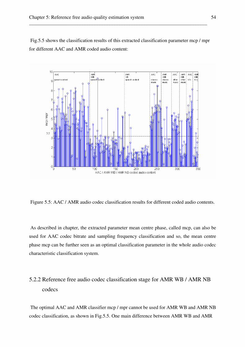
Chapter 5: Reference free audio quality estimation system ________________________________________________________________________
54
Fig.5.5 shows the classification results of this extracted classification parameter mcp / mpr
for different AAC and AMR coded audio content:
Figure 5.5: AAC / AMR audio codec classification results for different coded audio contents.
As described in chapter, the extracted parameter mean centre phase, called mcp, can also be
used for AAC codec bitrate and sampling frequency classification and so, the mean centre
phase mcp can be further seen as an optimal classification parameter in the whole audio codec
characteristic classification system.
5.2.2 Reference free audio codec classification stage for AMR WB / AMR NB
codecs
The optimal AAC and AMR classifier mcp / mpr cannot be used for AMR WB and AMR NB
codec classification, as shown in Fig.5.5. One main difference between AMR WB and AMR
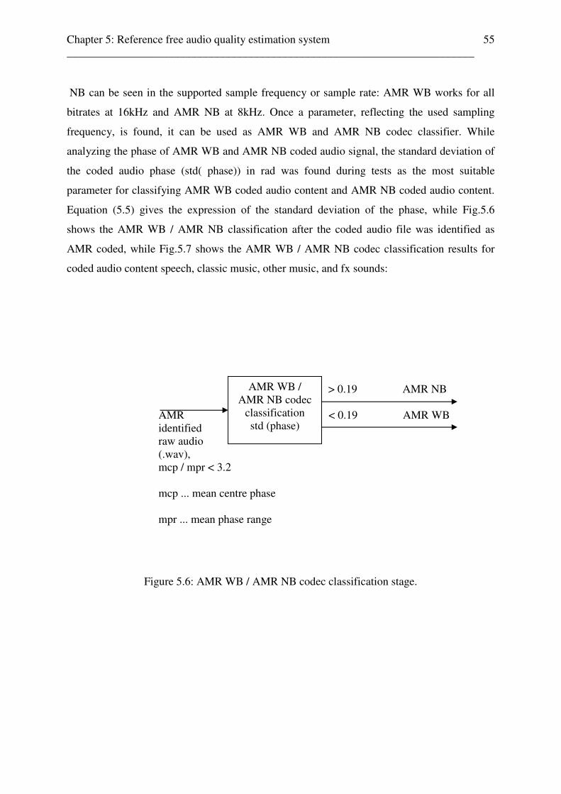
Chapter 5: Reference free audio quality estimation system ________________________________________________________________________
55
NB can be seen in the supported sample frequency or sample rate: AMR WB works for all
bitrates at 16kHz and AMR NB at 8kHz. Once a parameter, reflecting the used sampling
frequency, is found, it can be used as AMR WB and AMR NB codec classifier. While
analyzing the phase of AMR WB and AMR NB coded audio signal, the standard deviation of
the coded audio phase (std( phase)) in rad was found during tests as the most suitable
parameter for classifying AMR WB coded audio content and AMR NB coded audio content.
Equation (5.5) gives the expression of the standard deviation of the phase, while Fig.5.6
shows the AMR WB / AMR NB classification after the coded audio file was identified as
AMR coded, while Fig.5.7 shows the AMR WB / AMR NB codec classification results for
coded audio content speech, classic music, other music, and fx sounds:
Figure 5.6: AMR WB / AMR NB codec classification stage.
AMR WB / AMR NB codec
classification std (phase)
> 0.19 AMR NB AMR < 0.19 AMR WB identified raw audio (.wav), mcp / mpr < 3.2 mcp ... mean centre phase mpr ... mean phase range
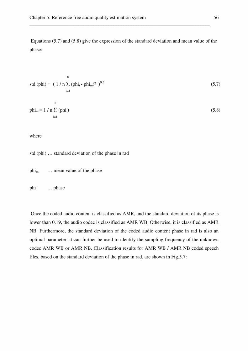
Chapter 5: Reference free audio quality estimation system ________________________________________________________________________
56
Equations (5.7) and (5.8) give the expression of the standard deviation and mean value of the
phase:
n
std (phi) = ( 1 / n ∑ (phii - phim)² )0.5 (5.7)
i=1
n
phim = 1 / n ∑ (phii) (5.8) i=1
where
std (phi) … standard deviation of the phase in rad
phim … mean value of the phase
phi … phase
Once the coded audio content is classified as AMR, and the standard deviation of its phase is
lower than 0.19, the audio codec is classified as AMR WB. Otherwise, it is classified as AMR
NB. Furthermore, the standard deviation of the coded audio content phase in rad is also an
optimal parameter: it can further be used to identify the sampling frequency of the unknown
codec AMR WB or AMR NB. Classification results for AMR WB / AMR NB coded speech
files, based on the standard deviation of the phase in rad, are shown in Fig.5.7:

Chapter 5: Reference free audio quality estimation system ________________________________________________________________________
57
Figure 5.7: AMR WB / AMR NB codec classification results for different coded speech
contents.
5.2.3 Reference free audio codec settings bitrate and sampling frequency
classification stage
For the prediction of the bitrates and sampling frequencies, the available audio codec settings
must be taken into account. For example, the sampling frequency of an AMR WB codec is
16kHz for every bitrate and 8kHz for every bitrate using AMR NB, while the sampling
frequencies in case of AAC can be individually chosen for every bitrate. So, the audio codec
classification of AMR WB or AMR NB determinates also the sampling frequencies, where in
case of AAC, the specific chosen sampling frequency can be classified by the optimal
parameter mean centre phase mcp, which is also used for the ratio of the mean centre phase
and mean phase range for the classification of AAC and AMR.
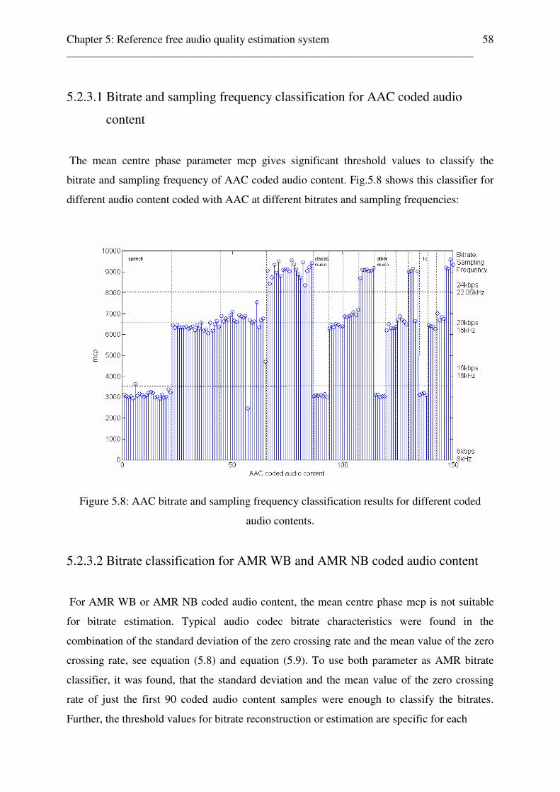
Chapter 5: Reference free audio quality estimation system ________________________________________________________________________
58
5.2.3.1 Bitrate and sampling frequency classification for AAC coded audio
content
The mean centre phase parameter mcp gives significant threshold values to classify the
bitrate and sampling frequency of AAC coded audio content. Fig.5.8 shows this classifier for
different audio content coded with AAC at different bitrates and sampling frequencies:
Figure 5.8: AAC bitrate and sampling frequency classification results for different coded
audio contents.
5.2.3.2 Bitrate classification for AMR WB and AMR NB coded audio content
For AMR WB or AMR NB coded audio content, the mean centre phase mcp is not suitable
for bitrate estimation. Typical audio codec bitrate characteristics were found in the
combination of the standard deviation of the zero crossing rate and the mean value of the zero
crossing rate, see equation (5.8) and equation (5.9). To use both parameter as AMR bitrate
classifier, it was found, that the standard deviation and the mean value of the zero crossing
rate of just the first 90 coded audio content samples were enough to classify the bitrates.
Further, the threshold values for bitrate reconstruction or estimation are specific for each
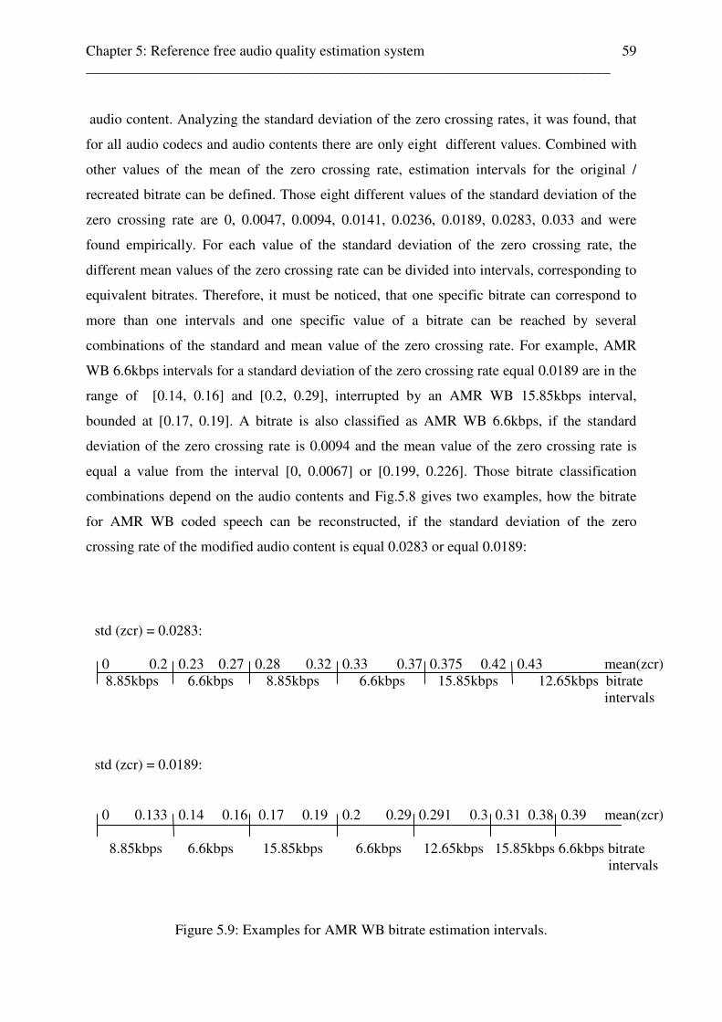
Chapter 5: Reference free audio quality estimation system ________________________________________________________________________
59
audio content. Analyzing the standard deviation of the zero crossing rates, it was found, that
for all audio codecs and audio contents there are only eight different values. Combined with
other values of the mean of the zero crossing rate, estimation intervals for the original /
recreated bitrate can be defined. Those eight different values of the standard deviation of the
zero crossing rate are 0, 0.0047, 0.0094, 0.0141, 0.0236, 0.0189, 0.0283, 0.033 and were
found empirically. For each value of the standard deviation of the zero crossing rate, the
different mean values of the zero crossing rate can be divided into intervals, corresponding to
equivalent bitrates. Therefore, it must be noticed, that one specific bitrate can correspond to
more than one intervals and one specific value of a bitrate can be reached by several
combinations of the standard and mean value of the zero crossing rate. For example, AMR
WB 6.6kbps intervals for a standard deviation of the zero crossing rate equal 0.0189 are in the
range of [0.14, 0.16] and [0.2, 0.29], interrupted by an AMR WB 15.85kbps interval,
bounded at [0.17, 0.19]. A bitrate is also classified as AMR WB 6.6kbps, if the standard
deviation of the zero crossing rate is 0.0094 and the mean value of the zero crossing rate is
equal a value from the interval [0, 0.0067] or [0.199, 0.226]. Those bitrate classification
combinations depend on the audio contents and Fig.5.8 gives two examples, how the bitrate
for AMR WB coded speech can be reconstructed, if the standard deviation of the zero
crossing rate of the modified audio content is equal 0.0283 or equal 0.0189:
Figure 5.9: Examples for AMR WB bitrate estimation intervals.
std (zcr) = 0.0283: 0 0.2 0.23 0.27 0.28 0.32 0.33 0.37 0.375 0.42 0.43 mean(zcr) 8.85kbps 6.6kbps 8.85kbps 6.6kbps 15.85kbps 12.65kbps bitrate intervals std (zcr) = 0.0189: 0 0.133 0.14 0.16 0.17 0.19 0.2 0.29 0.291 0.3 0.31 0.38 0.39 mean(zcr) 8.85kbps 6.6kbps 15.85kbps 6.6kbps 12.65kbps 15.85kbps 6.6kbps bitrate intervals
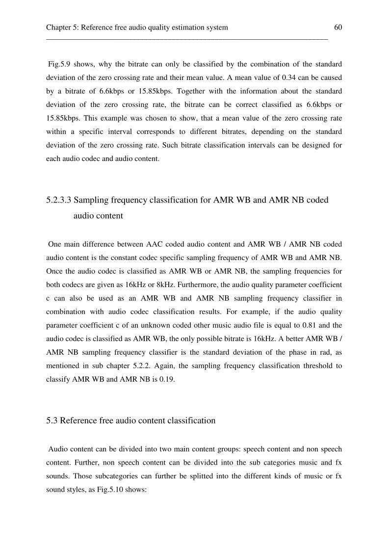
Chapter 5: Reference free audio quality estimation system ________________________________________________________________________
60
Fig.5.9 shows, why the bitrate can only be classified by the combination of the standard
deviation of the zero crossing rate and their mean value. A mean value of 0.34 can be caused
by a bitrate of 6.6kbps or 15.85kbps. Together with the information about the standard
deviation of the zero crossing rate, the bitrate can be correct classified as 6.6kbps or
15.85kbps. This example was chosen to show, that a mean value of the zero crossing rate
within a specific interval corresponds to different bitrates, depending on the standard
deviation of the zero crossing rate. Such bitrate classification intervals can be designed for
each audio codec and audio content.
5.2.3.3 Sampling frequency classification for AMR WB and AMR NB coded
audio content
One main difference between AAC coded audio content and AMR WB / AMR NB coded
audio content is the constant codec specific sampling frequency of AMR WB and AMR NB.
Once the audio codec is classified as AMR WB or AMR NB, the sampling frequencies for
both codecs are given as 16kHz or 8kHz. Furthermore, the audio quality parameter coefficient
c can also be used as an AMR WB and AMR NB sampling frequency classifier in
combination with audio codec classification results. For example, if the audio quality
parameter coefficient c of an unknown coded other music audio file is equal to 0.81 and the
audio codec is classified as AMR WB, the only possible bitrate is 16kHz. A better AMR WB /
AMR NB sampling frequency classifier is the standard deviation of the phase in rad, as
mentioned in sub chapter 5.2.2. Again, the sampling frequency classification threshold to
classify AMR WB and AMR NB is 0.19.
5.3 Reference free audio content classification
Audio content can be divided into two main content groups: speech content and non speech
content. Further, non speech content can be divided into the sub categories music and fx
sounds. Those subcategories can further be splitted into the different kinds of music or fx
sound styles, as Fig.5.10 shows:
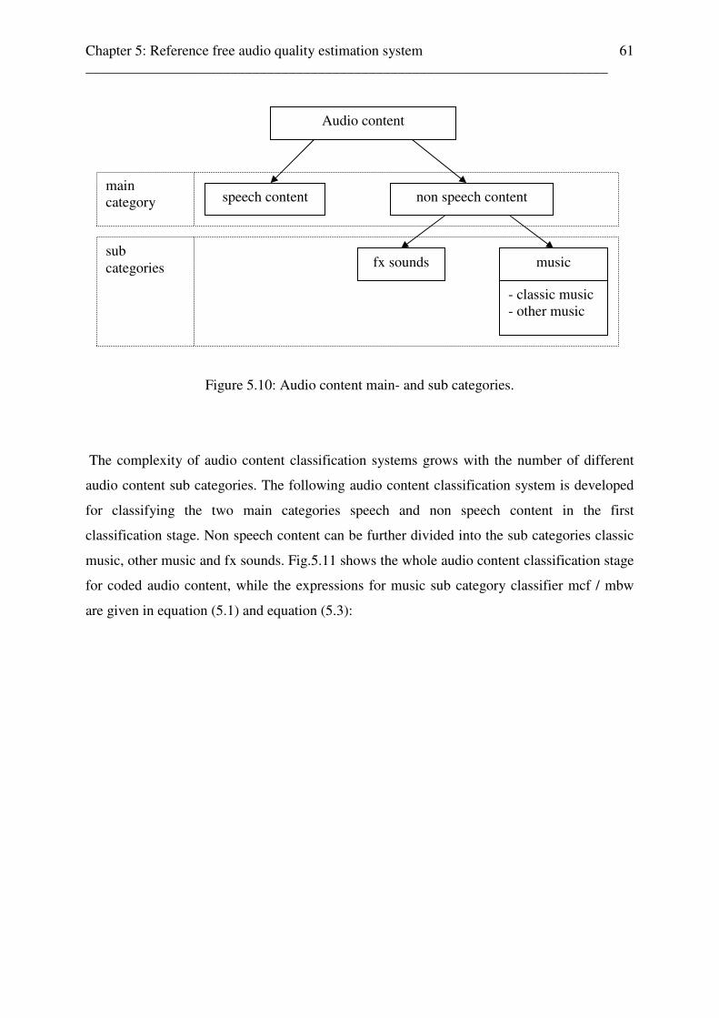
Chapter 5: Reference free audio quality estimation system ________________________________________________________________________
61
Figure 5.10: Audio content main- and sub categories.
The complexity of audio content classification systems grows with the number of different
audio content sub categories. The following audio content classification system is developed
for classifying the two main categories speech and non speech content in the first
classification stage. Non speech content can be further divided into the sub categories classic
music, other music and fx sounds. Fig.5.11 shows the whole audio content classification stage
for coded audio content, while the expressions for music sub category classifier mcf / mbw
are given in equation (5.1) and equation (5.3):
Audio content
speech content non speech content
fx sounds music
- classic music - other music
main category
sub categories

Chapter 5: Reference free audio quality estimation system ________________________________________________________________________
62
Figure 5.11: Audio content classification stage for coded audio content.
5.3.1 Reference free audio content classification for coded speech and non
speech content
For developing an audio content classifier for coded audio content, based on time domain
characteristics (zero crossing rate classifier), the audio codec specific characteristics in
relation to their zero crossing points must be taken into account. To divide AAC from AMR
coded audio content using zero crossing rate classification, a further audio signal forming
process is necessary to make sure, that even AAC coded news speaker scenarios are classified
as speech content. Audio content coded by AAC codec is characterized by extra samples
introduced by this audio codec. Those samples influence the standard deviation of the zero
crossing rate. So, an AAC coded speech file is characterized by a more periodic form of the
zero crossing rate in a specific range and will be classified as non speech content. For a better
Audio content classification stage for coded speech and non speech content std (zcr_mod)
Audio content classification stage for coded non speech content mean (zcr)
Audio content classification for coded music content (mcf / mbw)
> 0.13 speech raw audio (.wav) < 0.13 0.23 < mean(zcr) < 0.53 fx sounds < 0.23 > 0.59 classic music < 0.59 other music raw audio ............. unknown coded audio content (AAC / AMR WB /AMR NB) std (zcr_mod) ....... standard deviation of the zero crossing rate of the modified audio file mean (zcr_mod) ... mean value of the zero crossing rate of the modified audio file mcf / mbw ............ mean centre frequency and mean bandwidth of the unmodified audio file
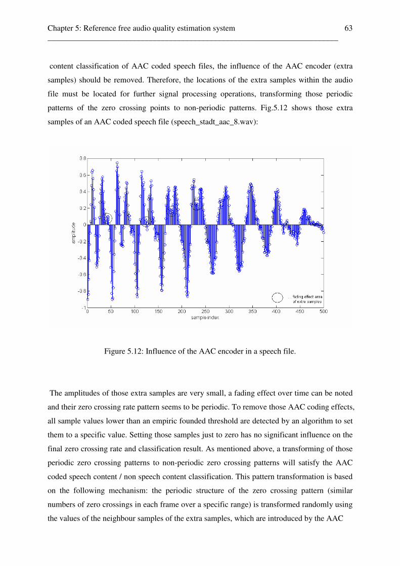
Chapter 5: Reference free audio quality estimation system ________________________________________________________________________
63
content classification of AAC coded speech files, the influence of the AAC encoder (extra
samples) should be removed. Therefore, the locations of the extra samples within the audio
file must be located for further signal processing operations, transforming those periodic
patterns of the zero crossing points to non-periodic patterns. Fig.5.12 shows those extra
samples of an AAC coded speech file (speech_stadt_aac_8.wav):
Figure 5.12: Influence of the AAC encoder in a speech file.
The amplitudes of those extra samples are very small, a fading effect over time can be noted
and their zero crossing rate pattern seems to be periodic. To remove those AAC coding effects,
all sample values lower than an empiric founded threshold are detected by an algorithm to set
them to a specific value. Setting those samples just to zero has no significant influence on the
final zero crossing rate and classification result. As mentioned above, a transforming of those
periodic zero crossing patterns to non-periodic zero crossing patterns will satisfy the AAC
coded speech content / non speech content classification. This pattern transformation is based
on the following mechanism: the periodic structure of the zero crossing pattern (similar
numbers of zero crossings in each frame over a specific range) is transformed randomly using
the values of the neighbour samples of the extra samples, which are introduced by the AAC

Chapter 5: Reference free audio quality estimation system ________________________________________________________________________
64
encoder. While such time discrete signals also consists of negative sample values, a complex
signal sample substitution at a specific time point solves the classification process of AAC
coded speech best. The so modified AAC coded speech file, presented in the time domain, is
given in Fig.5.13, while the transformation process is expressed in (5.10):
x(i) = √(x(i-2))| (5.10)
0 < x(i) < 0.1
where
x(i) … audio sample at time index i
x(i-2) … audio sample at time index i-2
Equation (5.10) shows, that the amplitude of the audio file at time point i is substituted by the
value of the square root of the amplitude of the same audio file at time point i-2, if the
amplitude at time point i is in the range [0, 0.1], which can also be seen in Fig. 5.13:
Figure 5.13: Modified speech signal in the time domain.
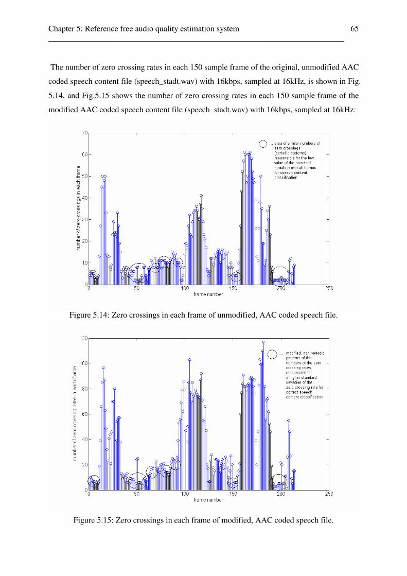
Chapter 5: Reference free audio quality estimation system ________________________________________________________________________
65
The number of zero crossing rates in each 150 sample frame of the original, unmodified AAC
coded speech content file (speech_stadt.wav) with 16kbps, sampled at 16kHz, is shown in Fig.
5.14, and Fig.5.15 shows the number of zero crossing rates in each 150 sample frame of the
modified AAC coded speech content file (speech_stadt.wav) with 16kbps, sampled at 16kHz:
Figure 5.14: Zero crossings in each frame of unmodified, AAC coded speech file.
Figure 5.15: Zero crossings in each frame of modified, AAC coded speech file.

Chapter 5: Reference free audio quality estimation system ________________________________________________________________________
66
Comparing the results from Fig.5.14 with those from Fig.5.15, it can be seen, that the
periodic pattern of the numbers of zero crossings for the case of the unmodified audio file are
transformed to non periodic patterns in the case of the modified audio file, which leads to a
higher standard deviation of the zero crossing rate resulting in a correct audio content
classification for coded speech files. Further, comparing the results in Fig.5.14 and Fig.5.15,
the numbers of the zero crossing rates in the marked areas of the modified audio file differs
more from frame to frame, leading to a higher mean value of the standard deviation of the
zero crossing rate over all frames than for the case of the original, unmodified audio file. Fig.
5.16 shows the number of zero crossings in each frame of a modified AMR WB coded speech
file:
Figure 5.16: Number of zero crossings in each frame of a modified AMR WB coded speech
file.
The following audio content classification process is done by this so transformed or modified
audio signal, all other classification processes are based on the untransformed or unmodified
audio signal. Using the mechanism from sub chapter 3.2 for uncoded audio content

Chapter 5: Reference free audio quality estimation system ________________________________________________________________________
67
classification, the audio signal modification of the coded audio file and a threshold value
variation of the standard deviation of the zero crossing rate to 0.13 enables the audio content
classification of different coded audio content, codec independently.
An overview over the classification results of the unmodified and modified AAC coded
speech file with codec settings 8kbps and 8kHz is given in Table 5.1:
AAC coded speech file std (zcr) classified as
Unmodified 0.0648 non speech content
Modified 0.1775 Speech content
Table 5.1: Audio content classification result for unmodified and modified AAC coded speech
file
As Table 5.1 shows, the standard deviation of the unmodified AAC coded speech file with
audio codec settings 16kbps and 16kHz is equal 0.0648 and would be classified as non speech
content. The standard deviation of the modified AAC coded speech file with the same audio
codec settings is equal 0.1775 and correctly classified as speech. This classification
mechanism is shown in Fig.5.17, while Fig.5.18 shows the results of this classification for
different coded speech and non speech content:
raw audio ... unknown coded audio content (AAC / AMR WB / AMR NB)
std (zcr_mod) ... standard deviation of the zero crossing rate of the modified audio
file
Figure 5.17: Main audio content classification stage of the reference free audio quality
estimation system for different coded audio content
Audio content classification for
coded speech and non-speech content
std (zcr_mod)
raw audio (.wav)
> 0.13 speech content
< 0.13 non speech content
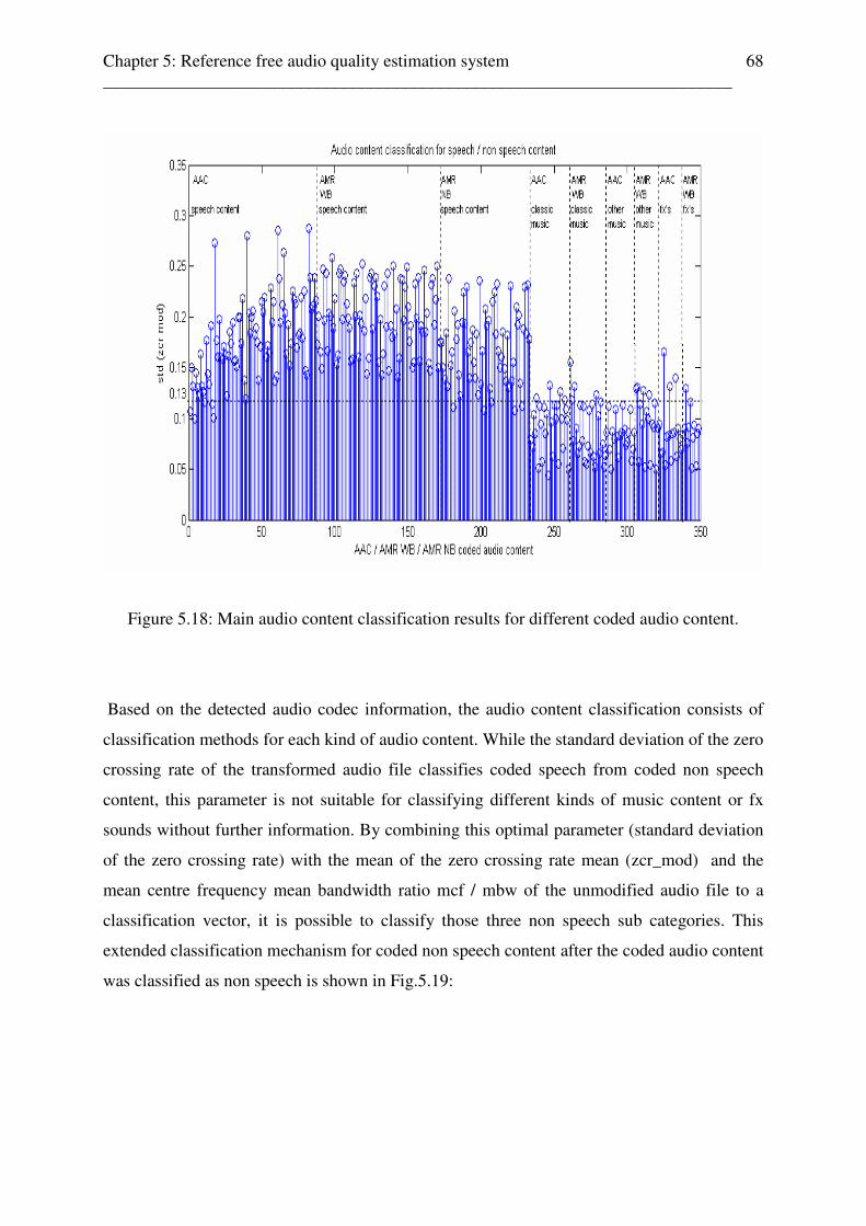
Chapter 5: Reference free audio quality estimation system ________________________________________________________________________
68
Figure 5.18: Main audio content classification results for different coded audio content.
Based on the detected audio codec information, the audio content classification consists of
classification methods for each kind of audio content. While the standard deviation of the zero
crossing rate of the transformed audio file classifies coded speech from coded non speech
content, this parameter is not suitable for classifying different kinds of music content or fx
sounds without further information. By combining this optimal parameter (standard deviation
of the zero crossing rate) with the mean of the zero crossing rate mean (zcr_mod) and the
mean centre frequency mean bandwidth ratio mcf / mbw of the unmodified audio file to a
classification vector, it is possible to classify those three non speech sub categories. This
extended classification mechanism for coded non speech content after the coded audio content
was classified as non speech is shown in Fig.5.19:
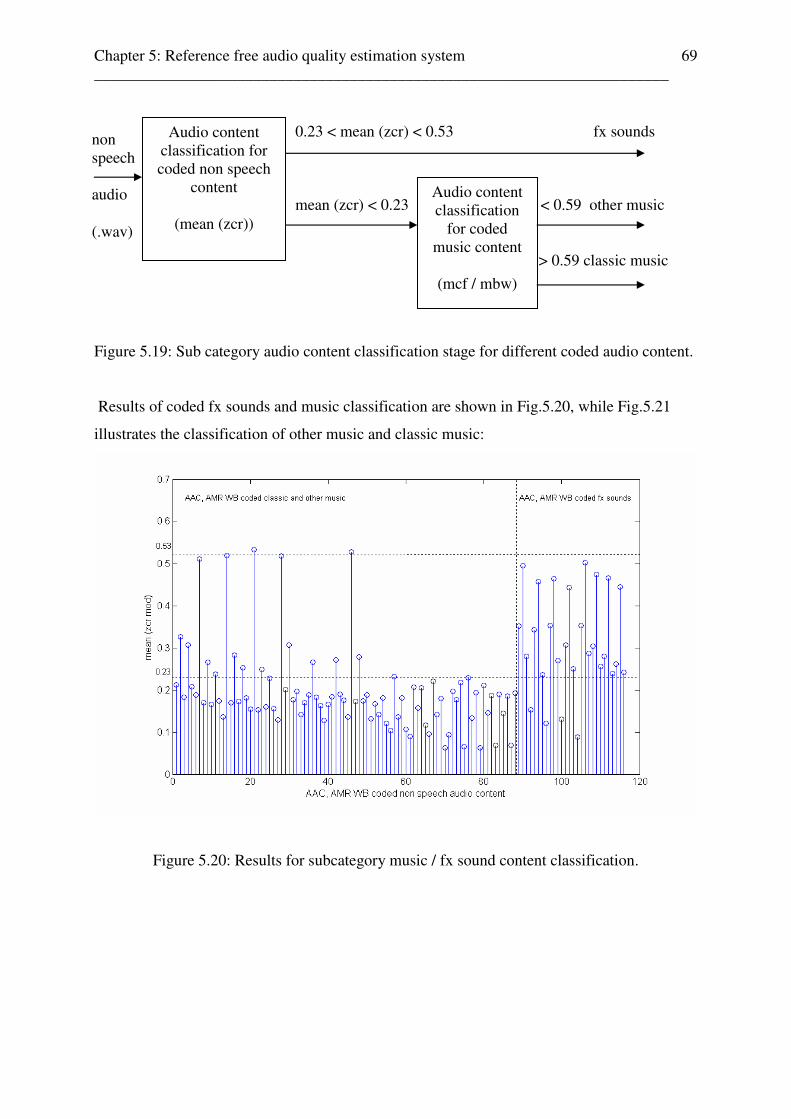
Chapter 5: Reference free audio quality estimation system ________________________________________________________________________
69
Figure 5.19: Sub category audio content classification stage for different coded audio content.
Results of coded fx sounds and music classification are shown in Fig.5.20, while Fig.5.21
illustrates the classification of other music and classic music:
Figure 5.20: Results for subcategory music / fx sound content classification.
Audio content classification for coded non speech
content
(mean (zcr))
Audio content classification
for coded music content
(mcf / mbw)
0.23 < mean (zcr) < 0.53 fx sounds mean (zcr) < 0.23 < 0.59 other music > 0.59 classic music
non speech audio (.wav)
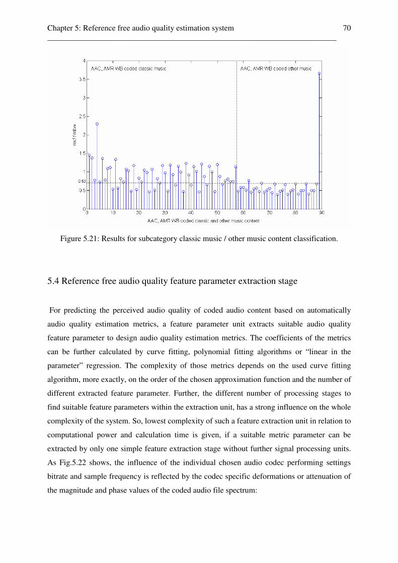
Chapter 5: Reference free audio quality estimation system ________________________________________________________________________
70
Figure 5.21: Results for subcategory classic music / other music content classification.
5.4 Reference free audio quality feature parameter extraction stage
For predicting the perceived audio quality of coded audio content based on automatically
audio quality estimation metrics, a feature parameter unit extracts suitable audio quality
feature parameter to design audio quality estimation metrics. The coefficients of the metrics
can be further calculated by curve fitting, polynomial fitting algorithms or “linear in the
parameter” regression. The complexity of those metrics depends on the used curve fitting
algorithm, more exactly, on the order of the chosen approximation function and the number of
different extracted feature parameter. Further, the different number of processing stages to
find suitable feature parameters within the extraction unit, has a strong influence on the whole
complexity of the system. So, lowest complexity of such a feature extraction unit in relation to
computational power and calculation time is given, if a suitable metric parameter can be
extracted by only one simple feature extraction stage without further signal processing units.
As Fig.5.22 shows, the influence of the individual chosen audio codec performing settings
bitrate and sample frequency is reflected by the codec specific deformations or attenuation of
the magnitude and phase values of the coded audio file spectrum:
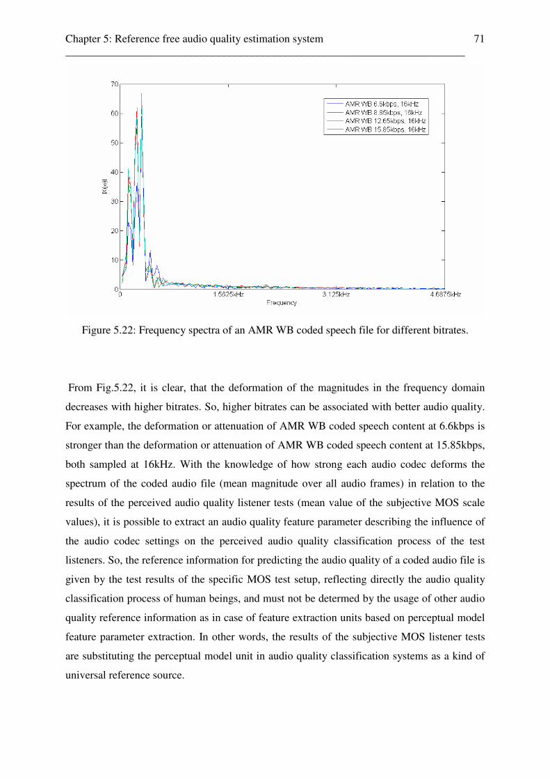
Chapter 5: Reference free audio quality estimation system ________________________________________________________________________
71
Figure 5.22: Frequency spectra of an AMR WB coded speech file for different bitrates.
From Fig.5.22, it is clear, that the deformation of the magnitudes in the frequency domain
decreases with higher bitrates. So, higher bitrates can be associated with better audio quality.
For example, the deformation or attenuation of AMR WB coded speech content at 6.6kbps is
stronger than the deformation or attenuation of AMR WB coded speech content at 15.85kbps,
both sampled at 16kHz. With the knowledge of how strong each audio codec deforms the
spectrum of the coded audio file (mean magnitude over all audio frames) in relation to the
results of the perceived audio quality listener tests (mean value of the subjective MOS scale
values), it is possible to extract an audio quality feature parameter describing the influence of
the audio codec settings on the perceived audio quality classification process of the test
listeners. So, the reference information for predicting the audio quality of a coded audio file is
given by the test results of the specific MOS test setup, reflecting directly the audio quality
classification process of human beings, and must not be determed by the usage of other audio
quality reference information as in case of feature extraction units based on perceptual model
feature parameter extraction. In other words, the results of the subjective MOS listener tests
are substituting the perceptual model unit in audio quality classification systems as a kind of
universal reference source.
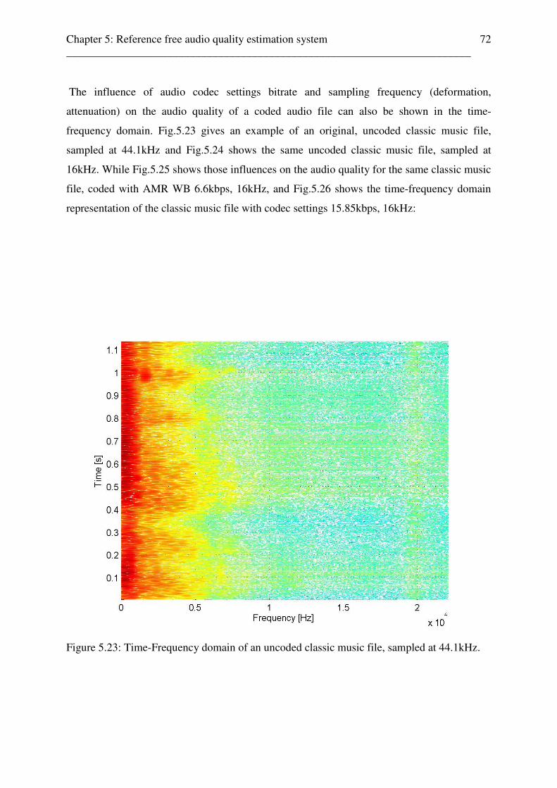
Chapter 5: Reference free audio quality estimation system ________________________________________________________________________
72
The influence of audio codec settings bitrate and sampling frequency (deformation,
attenuation) on the audio quality of a coded audio file can also be shown in the time-
frequency domain. Fig.5.23 gives an example of an original, uncoded classic music file,
sampled at 44.1kHz and Fig.5.24 shows the same uncoded classic music file, sampled at
16kHz. While Fig.5.25 shows those influences on the audio quality for the same classic music
file, coded with AMR WB 6.6kbps, 16kHz, and Fig.5.26 shows the time-frequency domain
representation of the classic music file with codec settings 15.85kbps, 16kHz:
Figure 5.23: Time-Frequency domain of an uncoded classic music file, sampled at 44.1kHz.
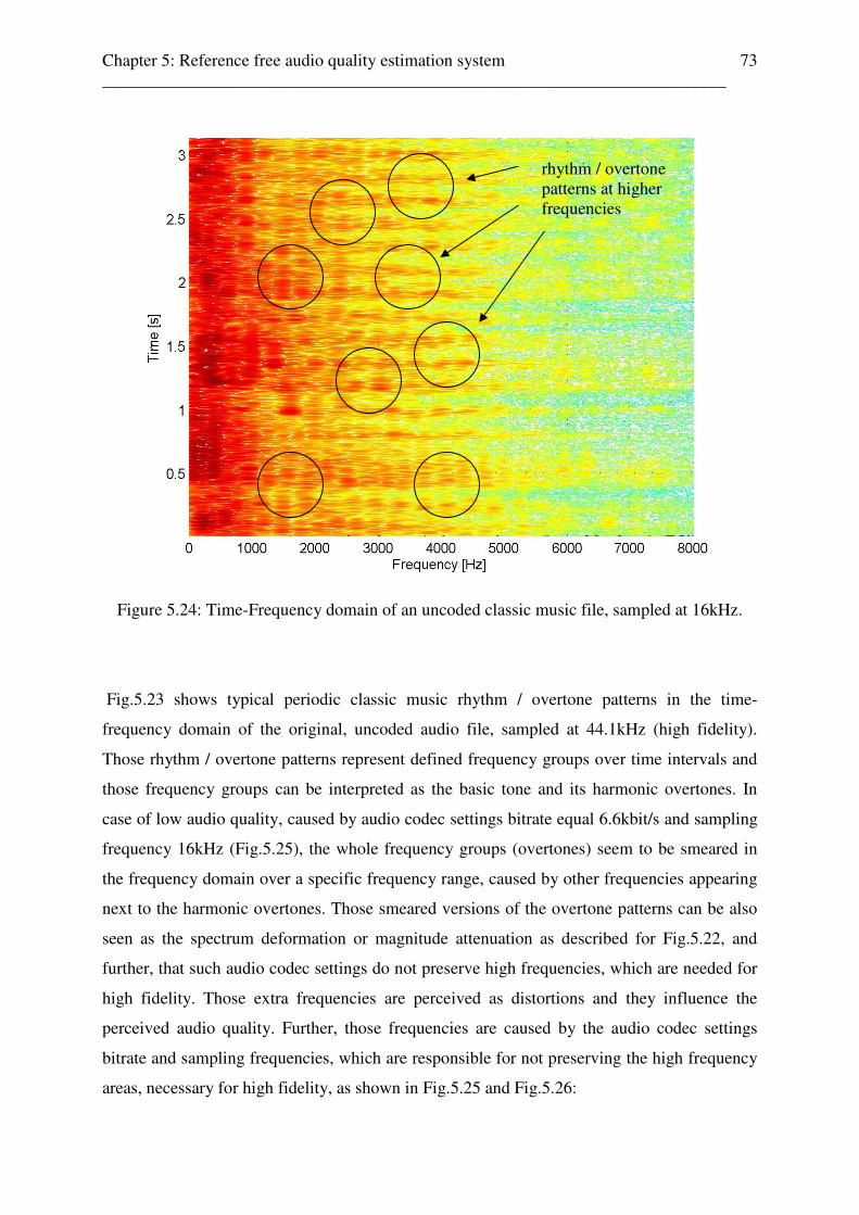
Chapter 5: Reference free audio quality estimation system ________________________________________________________________________
73
Figure 5.24: Time-Frequency domain of an uncoded classic music file, sampled at 16kHz.
Fig.5.23 shows typical periodic classic music rhythm / overtone patterns in the time-
frequency domain of the original, uncoded audio file, sampled at 44.1kHz (high fidelity).
Those rhythm / overtone patterns represent defined frequency groups over time intervals and
those frequency groups can be interpreted as the basic tone and its harmonic overtones. In
case of low audio quality, caused by audio codec settings bitrate equal 6.6kbit/s and sampling
frequency 16kHz (Fig.5.25), the whole frequency groups (overtones) seem to be smeared in
the frequency domain over a specific frequency range, caused by other frequencies appearing
next to the harmonic overtones. Those smeared versions of the overtone patterns can be also
seen as the spectrum deformation or magnitude attenuation as described for Fig.5.22, and
further, that such audio codec settings do not preserve high frequencies, which are needed for
high fidelity. Those extra frequencies are perceived as distortions and they influence the
perceived audio quality. Further, those frequencies are caused by the audio codec settings
bitrate and sampling frequencies, which are responsible for not preserving the high frequency
areas, necessary for high fidelity, as shown in Fig.5.25 and Fig.5.26:
rhythm / overtone patterns at higher frequencies
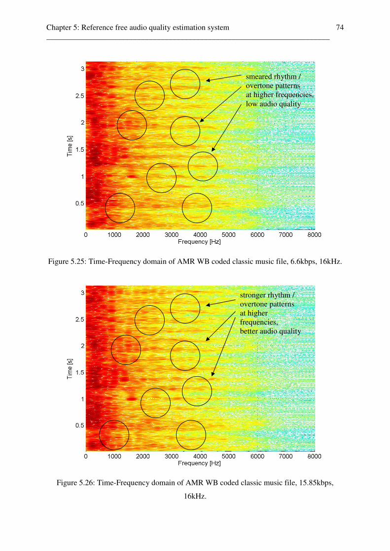
Chapter 5: Reference free audio quality estimation system ________________________________________________________________________
74
Figure 5.25: Time-Frequency domain of AMR WB coded classic music file, 6.6kbps, 16kHz.
Figure 5.26: Time-Frequency domain of AMR WB coded classic music file, 15.85kbps,
16kHz.
stronger rhythm / overtone patterns at higher frequencies, better audio quality
smeared rhythm / overtone patterns at higher frequencies, low audio quality
Chapter 5: Reference free audio quality estimation system ________________________________________________________________________
75
The low audio quality of an AMR WB coded classic music with codec settings 6.6kbps,
16kHz can be seen in the smeared rhythm / overtone pattern in the time-frequency domain,
while for AMR WB 15.85kbps, 16kHz, the ranges of those smeared rhythm patterns are
smaller, leading to a higher audio quality. Finally, it can be said, that low audio quality
corresponds with a strong smeared audio spectrum (strong deformation and attenuation), and
higher audio quality with a lesser smeared audio spectrum (lower deformation and attenuation,
higher frequencies are preserved).
For analyzing the frequency domain characteristic of time signals, first step in the signal
processing algorithm is a Fast Fourier Transformation FFT, representing the time signal by its
frequency domain characteristics magnitude and phase components. While all kind of audio
signals are divided into frames of different length for audio signal processing and analyzing,
mean values, like the mean magnitude, mean centre frequency or mean bandwidth over all
frames of a coded audio file can be calculated and extracted as feature parameter, resulting in
a single scalar value. The calculation complexity of suitable audio quality feature parameter
grows then with the number of necessary further signal operation processes to extract them.
For example, the feature extraction process of mean centre frequency and bandwidth is more
complex than the feature process extracting the mean value of the magnitude of the spectrum
of a coded audio file. This means, that the calculation of the mean centre frequency and mean
bandwidth needs more calculation operations than the calculation of the mean magnitude. In
that sense, the mean value of the magnitude over all frames of a coded audio file spectrum can
be seen as an optimal audio quality feature parameter for audio quality metric design. Once
such feature parameter, optimal or not, are found, they can be used as the parameter in audio
quality estimation design. The simplest model for an audio quality estimation metric to
predict the perceived audio quality of an unknown coded audio file without reference is a
linear equation of the form
MOSApred = c · p, (5.1)
with
c ... audio quality parameter coefficient c
p ... audio quality feature parameter p
Chapter 5: Reference free audio quality estimation system ________________________________________________________________________
76
Furthermore, this model can be seen as a reduced audio quality estimation metric, consisting
of only one audio feature parameter p and its audio quality parameter coefficient c.
This is possible, if an audio quality feature parameter can be found, that reflects the mean of
the subjective MOS scale values in a linear way. Then, the audio quality metric can be
reduced to an audio quality equation, consisting of only one optimal feature parameter of first
order with just one parameter coefficient. While the left side of the equation MOSApred can be
substituted by the mean value of the MOS scale value for each coded content type, given by
the subjective MOS test results, one specific audio quality parameter coefficient for each kind
of different coded audio content can be expressed by the following ratio:
c = mean (MOSsubj) / p (5.2)
5.4.1 Reference free audio quality parameter c to MOS scale value mapping unit
One specific audio quality parameter coefficient c can be seen as an element of an audio
codec setting and audio content specific interval, where the interval bounds are given by the
chosen audio codec settings bitrate and sampling frequency, depending on the audio content.
Those intervals are further used for mapping the audio quality parameter coefficient c to the
rounded mean value of the corresponding subjective MOS. A test setup of different coded
audio content, consisting of 349 different coded audio files, was used to find those significant
interval bounds. Fig.5.27 gives an example for the mapping intervals of AAC coded speech
content:
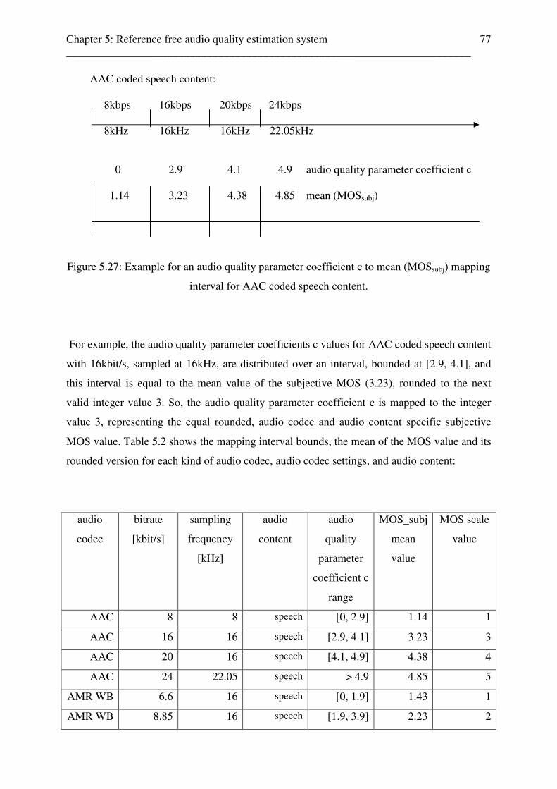
Chapter 5: Reference free audio quality estimation system ________________________________________________________________________
77
Figure 5.27: Example for an audio quality parameter coefficient c to mean (MOSsubj) mapping
interval for AAC coded speech content.
For example, the audio quality parameter coefficients c values for AAC coded speech content
with 16kbit/s, sampled at 16kHz, are distributed over an interval, bounded at [2.9, 4.1], and
this interval is equal to the mean value of the subjective MOS (3.23), rounded to the next
valid integer value 3. So, the audio quality parameter coefficient c is mapped to the integer
value 3, representing the equal rounded, audio codec and audio content specific subjective
MOS value. Table 5.2 shows the mapping interval bounds, the mean of the MOS value and its
rounded version for each kind of audio codec, audio codec settings, and audio content:
audio
codec
bitrate
[kbit/s]
sampling
frequency
[kHz]
audio
content
audio
quality
parameter
coefficient c
range
MOS_subj
mean
value
MOS scale
value
AAC 8 8 speech [0, 2.9] 1.14 1
AAC 16 16 speech [2.9, 4.1] 3.23 3
AAC 20 16 speech [4.1, 4.9] 4.38 4
AAC 24 22.05 speech > 4.9 4.85 5
AMR WB 6.6 16 speech [0, 1.9] 1.43 1
AMR WB 8.85 16 speech [1.9, 3.9] 2.23 2
AAC coded speech content: 8kbps 16kbps 20kbps 24kbps 8kHz 16kHz 16kHz 22.05kHz 0 2.9 4.1 4.9 audio quality parameter coefficient c 1.14 3.23 4.38 4.85 mean (MOSsubj)
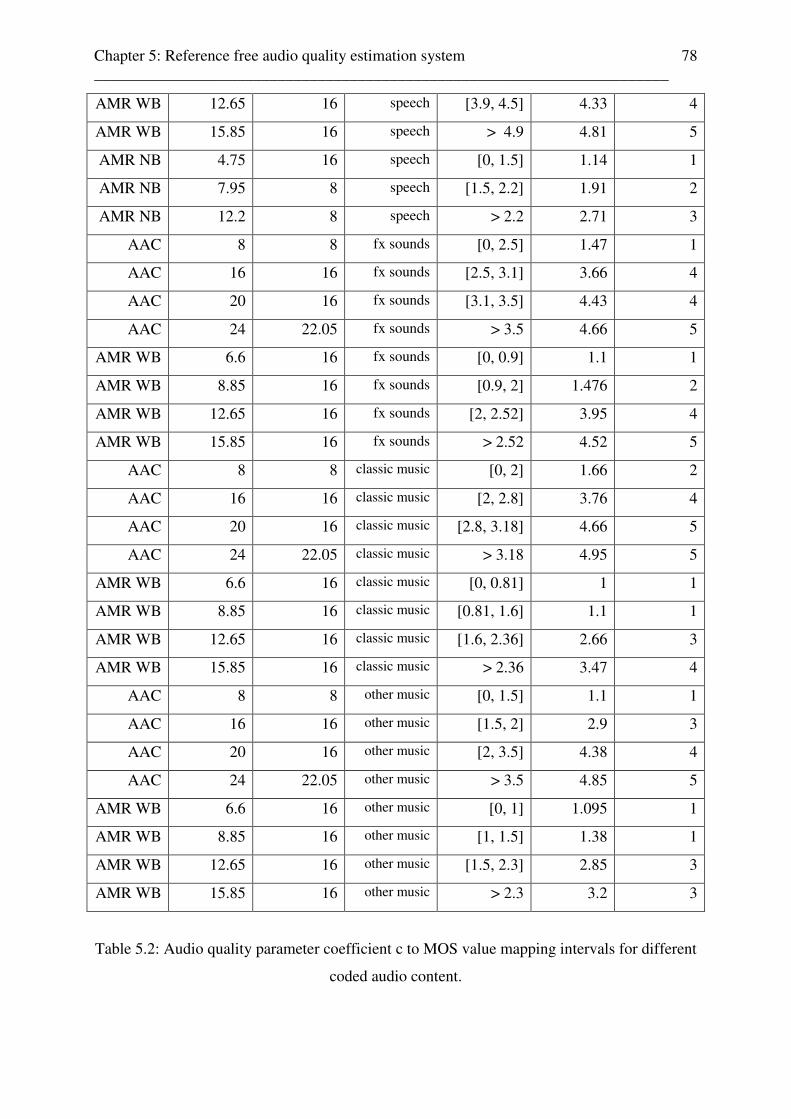
Chapter 5: Reference free audio quality estimation system ________________________________________________________________________
78
AMR WB 12.65 16 speech [3.9, 4.5] 4.33 4
AMR WB 15.85 16 speech > 4.9 4.81 5
AMR NB 4.75 16 speech [0, 1.5] 1.14 1
AMR NB 7.95 8 speech [1.5, 2.2] 1.91 2
AMR NB 12.2 8 speech > 2.2 2.71 3
AAC 8 8 fx sounds [0, 2.5] 1.47 1
AAC 16 16 fx sounds [2.5, 3.1] 3.66 4
AAC 20 16 fx sounds [3.1, 3.5] 4.43 4
AAC 24 22.05 fx sounds > 3.5 4.66 5
AMR WB 6.6 16 fx sounds [0, 0.9] 1.1 1
AMR WB 8.85 16 fx sounds [0.9, 2] 1.476 2
AMR WB 12.65 16 fx sounds [2, 2.52] 3.95 4
AMR WB 15.85 16 fx sounds > 2.52 4.52 5
AAC 8 8 classic music [0, 2] 1.66 2
AAC 16 16 classic music [2, 2.8] 3.76 4
AAC 20 16 classic music [2.8, 3.18] 4.66 5
AAC 24 22.05 classic music > 3.18 4.95 5
AMR WB 6.6 16 classic music [0, 0.81] 1 1
AMR WB 8.85 16 classic music [0.81, 1.6] 1.1 1
AMR WB 12.65 16 classic music [1.6, 2.36] 2.66 3
AMR WB 15.85 16 classic music > 2.36 3.47 4
AAC 8 8 other music [0, 1.5] 1.1 1
AAC 16 16 other music [1.5, 2] 2.9 3
AAC 20 16 other music [2, 3.5] 4.38 4
AAC 24 22.05 other music > 3.5 4.85 5
AMR WB 6.6 16 other music [0, 1] 1.095 1
AMR WB 8.85 16 other music [1, 1.5] 1.38 1
AMR WB 12.65 16 other music [1.5, 2.3] 2.85 3
AMR WB 15.85 16 other music > 2.3 3.2 3
Table 5.2: Audio quality parameter coefficient c to MOS value mapping intervals for different
coded audio content.
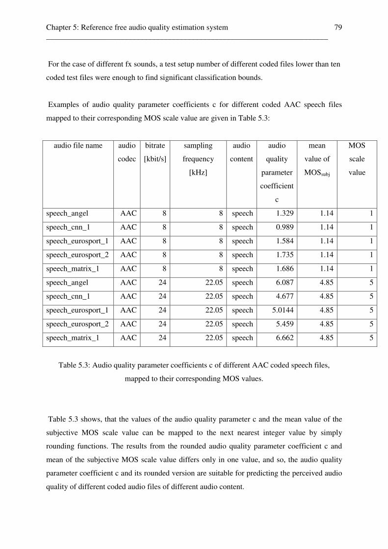
Chapter 5: Reference free audio quality estimation system ________________________________________________________________________
79
For the case of different fx sounds, a test setup number of different coded files lower than ten
coded test files were enough to find significant classification bounds.
Examples of audio quality parameter coefficients c for different coded AAC speech files
mapped to their corresponding MOS scale value are given in Table 5.3:
audio file name audio
codec
bitrate
[kbit/s]
sampling
frequency
[kHz]
audio
content
audio
quality
parameter
coefficient
c
mean
value of
MOSsubj
MOS
scale
value
speech_angel AAC 8 8 speech 1.329 1.14 1
speech_cnn_1 AAC 8 8 speech 0.989 1.14 1
speech_eurosport_1 AAC 8 8 speech 1.584 1.14 1
speech_eurosport_2 AAC 8 8 speech 1.735 1.14 1
speech_matrix_1 AAC 8 8 speech 1.686 1.14 1
speech_angel AAC 24 22.05 speech 6.087 4.85 5
speech_cnn_1 AAC 24 22.05 speech 4.677 4.85 5
speech_eurosport_1 AAC 24 22.05 speech 5.0144 4.85 5
speech_eurosport_2 AAC 24 22.05 speech 5.459 4.85 5
speech_matrix_1 AAC 24 22.05 speech 6.662 4.85 5
Table 5.3: Audio quality parameter coefficients c of different AAC coded speech files,
mapped to their corresponding MOS values.
Table 5.3 shows, that the values of the audio quality parameter c and the mean value of the
subjective MOS scale value can be mapped to the next nearest integer value by simply
rounding functions. The results from the rounded audio quality parameter coefficient c and
mean of the subjective MOS scale value differs only in one value, and so, the audio quality
parameter coefficient c and its rounded version are suitable for predicting the perceived audio
quality of different coded audio files of different audio content.
Chapter 5: Reference free audio quality estimation system ________________________________________________________________________
80
5.5 Reference free audio codec, audio codec settings, audio content, and audio
quality estimation results
The whole audio quality estimation system was implemented in MATLAB (cf. appendix C).
All MATLAB main programs and their syntax are given in Appendix C.3 - C.6 and the
performance of the whole reference free audio quality estimation system, consisting of an
audio codec classification stage, an audio codec setting estimation stage, an audio content
classification stage, and an audio quality estimation stage was proofed by the audio test file
setup given in Appendix C.2. All audio files (.wav) were chosen from audio codec setting
specific folders with the following syntax:
audio_codec\audio_codec_bitrate\content_name.wav
For example, the syntax of an AMR WB coded speech file with the audio codec settings
6.6kbps and sampling frequency 16kHz is
amr_wb\6600\speech_stadt.wav
This means, that all AMR WB coded audio files with bitrate 6.6kbps are stored in a folder
with path name amr_wb\6600\, all AMR WB coded audio files with bitrate 8.85kbps are
stored in a folder with the path name amr_wb\8850\, and so on. Following this specification,
it is possible to extract the whole information of audio codec, bitrate, and audio content from
this text string. Also, parts of this information string can be extracted to compare the
classification results with this kind of reference information about the test file. So, it is
possible to give detail results of the whole audio quality estimation process, for example, the
number of correct audio codec and audio bitrate classifications without information about the
predicted audio content and audio quality.

Chapter 5: Reference free audio quality estimation system ________________________________________________________________________
81
5.5.1 Reference free audio codec, audio codec settings, audio content, and audio
quality estimation results for unknown audio codec settings
Table 5.5 presents the precisions of each classification stage and Table 5.6 shows the results
of the vector interpretation, both for 349 different coded audio files (cf. appendix C.2.1):
classification stage number of precision
correct classification [%]
audio codec classification 326 93.41
audio codec bitrate classification 268 76.79
audio codec sampling frequency classification 347 99.43
audio content classification 288 82.52
audio quality estimation 246 70.49
Table 5.5: Precision of each classification stage for unknown audio codec settings.
vector representation number of
correct classification
precision
[%]
Correct MOS scale value 246 70.49
+/- one MOS value precision 72 20.63
Correct MOS scale value and +/- one MOS value
precision
318 91.12
Table 5.6: Correlation vector interpretation of the audio quality estimation results for 349
different coded audio files for unknown audio codec settings.
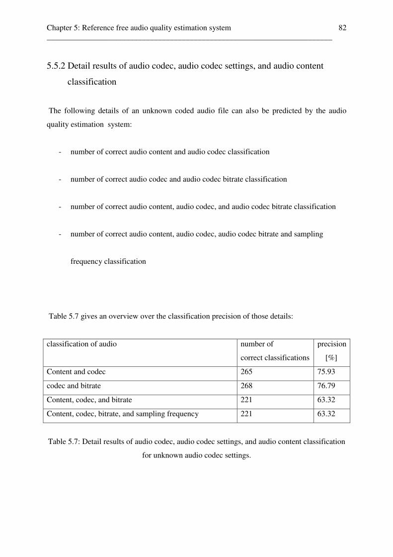
Chapter 5: Reference free audio quality estimation system ________________________________________________________________________
82
5.5.2 Detail results of audio codec, audio codec settings, and audio content
classification
The following details of an unknown coded audio file can also be predicted by the audio
quality estimation system:
- number of correct audio content and audio codec classification
- number of correct audio codec and audio codec bitrate classification
- number of correct audio content, audio codec, and audio codec bitrate classification
- number of correct audio content, audio codec, audio codec bitrate and sampling
frequency classification
Table 5.7 gives an overview over the classification precision of those details:
classification of audio number of
correct classifications
precision
[%]
Content and codec 265 75.93
codec and bitrate 268 76.79
Content, codec, and bitrate 221 63.32
Content, codec, bitrate, and sampling frequency 221 63.32
Table 5.7: Detail results of audio codec, audio codec settings, and audio content classification
for unknown audio codec settings.
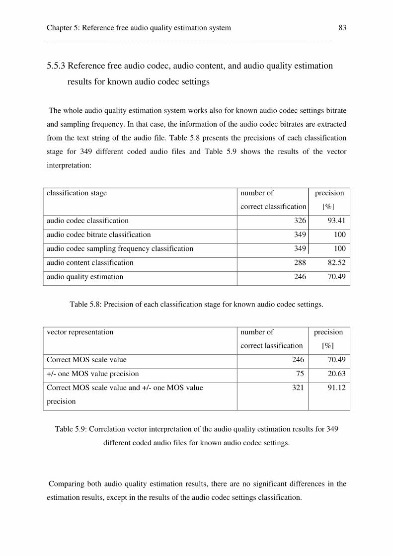
Chapter 5: Reference free audio quality estimation system ________________________________________________________________________
83
5.5.3 Reference free audio codec, audio content, and audio quality estimation
results for known audio codec settings
The whole audio quality estimation system works also for known audio codec settings bitrate
and sampling frequency. In that case, the information of the audio codec bitrates are extracted
from the text string of the audio file. Table 5.8 presents the precisions of each classification
stage for 349 different coded audio files and Table 5.9 shows the results of the vector
interpretation:
classification stage number of precision
correct classification [%]
audio codec classification 326 93.41
audio codec bitrate classification 349 100
audio codec sampling frequency classification 349 100
audio content classification 288 82.52
audio quality estimation 246 70.49
Table 5.8: Precision of each classification stage for known audio codec settings.
vector representation number of
correct lassification
precision
[%]
Correct MOS scale value 246 70.49
+/- one MOS value precision 75 20.63
Correct MOS scale value and +/- one MOS value
precision
321 91.12
Table 5.9: Correlation vector interpretation of the audio quality estimation results for 349
different coded audio files for known audio codec settings.
Comparing both audio quality estimation results, there are no significant differences in the
estimation results, except in the results of the audio codec settings classification.
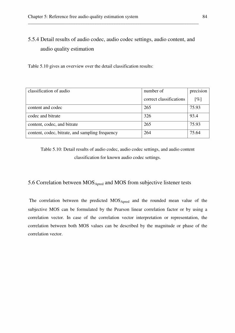
Chapter 5: Reference free audio quality estimation system ________________________________________________________________________
84
5.5.4 Detail results of audio codec, audio codec settings, audio content, and
audio quality estimation
Table 5.10 gives an overview over the detail classification results:
classification of audio number of
correct classifications
precision
[%]
content and codec 265 75.93
codec and bitrate 326 93.4
content, codec, and bitrate 265 75.93
content, codec, bitrate, and sampling frequency 264 75.64
Table 5.10: Detail results of audio codec, audio codec settings, and audio content
classification for known audio codec settings.
5.6 Correlation between MOSApred and MOS from subjective listener tests
The correlation between the predicted MOSApred and the rounded mean value of the
subjective MOS can be formulated by the Pearson linear correlation factor or by using a
correlation vector. In case of the correlation vector interpretation or representation, the
correlation between both MOS values can be described by the magnitude or phase of the
correlation vector.
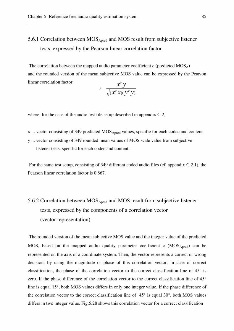
Chapter 5: Reference free audio quality estimation system ________________________________________________________________________
85
5.6.1 Correlation between MOSApred and MOS result from subjective listener
tests, expressed by the Pearson linear correlation factor
The correlation between the mapped audio parameter coefficient c (predicted MOSA)
and the rounded version of the mean subjective MOS value can be expressed by the Pearson
linear correlation factor:
where, for the case of the audio test file setup described in appendix C.2,
x ... vector consisting of 349 predicted MOSApred values, specific for each codec and content
y ... vector consisting of 349 rounded mean values of MOS scale value from subjective
listener tests, specific for each codec and content.
For the same test setup, consisting of 349 different coded audio files (cf. appendix C.2.1), the
Pearson linear correlation factor is 0.867.
5.6.2 Correlation between MOSApred and MOS result from subjective listener
tests, expressed by the components of a correlation vector
(vector representation)
The rounded version of the mean subjective MOS value and the integer value of the predicted
MOS, based on the mapped audio quality parameter coefficient c (MOSApred) can be
represented on the axis of a coordinate system. Then, the vector represents a correct or wrong
decision, by using the magnitude or phase of this correlation vector. In case of correct
classification, the phase of the correlation vector to the correct classification line of 45° is
zero. If the phase difference of the correlation vector to the correct classification line of 45°
line is equal 15°, both MOS values differs in only one integer value. If the phase difference of
the correlation vector to the correct classification line of 45° is equal 30°, both MOS values
differs in two integer value. Fig.5.28 shows this correlation vector for a correct classification
))(( yyxx
yxTT
T
r =
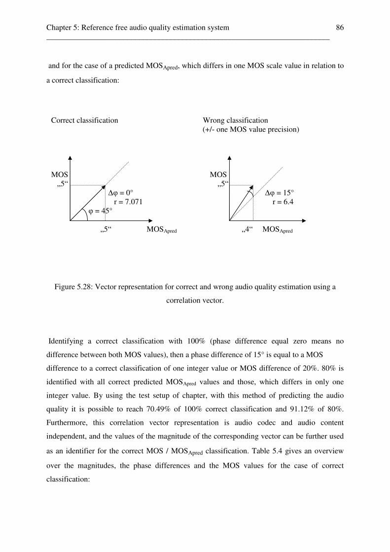
Chapter 5: Reference free audio quality estimation system ________________________________________________________________________
86
and for the case of a predicted MOSApred, which differs in one MOS scale value in relation to
a correct classification:
Figure 5.28: Vector representation for correct and wrong audio quality estimation using a
correlation vector.
Identifying a correct classification with 100% (phase difference equal zero means no
difference between both MOS values), then a phase difference of 15° is equal to a MOS
difference to a correct classification of one integer value or MOS difference of 20%. 80% is
identified with all correct predicted MOSApred values and those, which differs in only one
integer value. By using the test setup of chapter, with this method of predicting the audio
quality it is possible to reach 70.49% of 100% correct classification and 91.12% of 80%.
Furthermore, this correlation vector representation is audio codec and audio content
independent, and the values of the magnitude of the corresponding vector can be further used
as an identifier for the correct MOS / MOSApred classification. Table 5.4 gives an overview
over the magnitudes, the phase differences and the MOS values for the case of correct
classification:
Correct classification Wrong classification (+/- one MOS value precision) MOS MOS „5“ „5“ ∆φ = 0° ∆φ = 15° r = 7.071 r = 6.4 φ = 45° „5“ MOSApred „4“ MOSApred
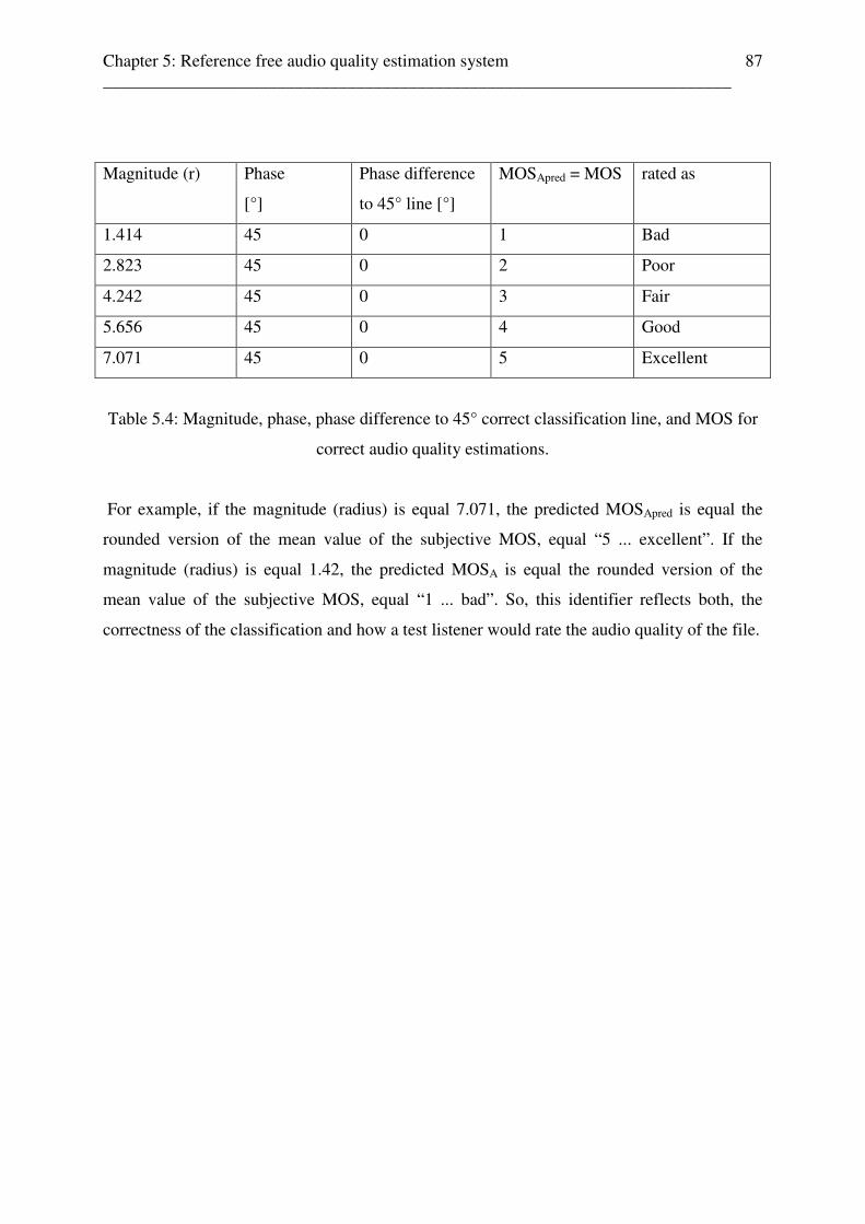
Chapter 5: Reference free audio quality estimation system ________________________________________________________________________
87
Magnitude (r) Phase
[°]
Phase difference
to 45° line [°]
MOSApred = MOS rated as
1.414 45 0 1 Bad
2.823 45 0 2 Poor
4.242 45 0 3 Fair
5.656 45 0 4 Good
7.071 45 0 5 Excellent
Table 5.4: Magnitude, phase, phase difference to 45° correct classification line, and MOS for
correct audio quality estimations.
For example, if the magnitude (radius) is equal 7.071, the predicted MOSApred is equal the
rounded version of the mean value of the subjective MOS, equal “5 ... excellent”. If the
magnitude (radius) is equal 1.42, the predicted MOSA is equal the rounded version of the
mean value of the subjective MOS, equal “1 ... bad”. So, this identifier reflects both, the
correctness of the classification and how a test listener would rate the audio quality of the file.

Chapter 5: Reference free audio quality estimation system ________________________________________________________________________
88
5.6 Classifier for reference free audio codec, audio codec settings, audio content,
and audio quality estimation, conclusion
All of the classifier within the reference free audio quality estimation system and their
threshold values are resumed in Table 5.5:
classification of Classifier threshold value
AAC / AMR mcp / mpr > 3.2 : AAC
AMR WB / AMR NB std (phase) > 0.19: AMR NB
AAC bitrate, sampling frequency Mcp see Fig. 5.81
AMR bitrate, sampling freqency mean(zcr), std(zcr) combination of both1
speech / non speech std (zcr_mod) > 0.13: speech
fx sound / music mean (zcr_mod) 0.23 < mean(zcr_mod) < 0.53
classic music / other music mcf / mbw > 0.59: classic music
MOSApred round(mean(MOSsubj))
mapped(mean(MOSsubj)/p)
mapped( c )
see Table 5.21
Table 5.5: Classifiers and threshold values for reference free audio codec, audio codec
settings, audio content, and audio quality estimation.
1) … classification based on more than one threshold values (intervals), of classifier
combinations, or codec and content specific classification / mapping intervals.
Chapter 6: Reference free audio codec, audio content, and audio quality estimation for audio sequences ________________________________________________________________________
89
Chapter 6
Reference free audio codec, audio content, and audio
quality estimation for audio sequences
The reference free audio quality estimation system can be extended to predict the audio
quality of each scene of a video sequence (video clip). Therefore, as described in chapter 3,
the whole audio track is divided into single audio scenes, depending on the scene change cut
time points or indexes, extracted by a scene detecting tool. This scene detecting tool is based
on the scene change time points of the video sequence. So, the audio content, audio codec, the
user specific audio codec settings bitrate and sampling frequency, and audio quality of each
scene can be predicted. In a video streaming scenario, the whole audio track of a video clip is
encoded by one specific audio codec with constant bitrate and sampling frequency. By using
the first scene of the audio sequence, audio codec and bitrate of the whole sequence can be
estimated.
- audio codec of the whole audio sequence
- audio codec bitrate of the whole audio sequence
Further, the following characteristics of each audio scene of the audio sequence are detectable:
- audio codec
- audio codec settings bitrate and sampling frequency
- audio content
- audio quality feature parameter p
Chapter 6: Reference free audio codec, audio content, and audio quality estimation for audio sequences ________________________________________________________________________
90
- audio quality feature parameter coefficient c
- MOSApred
- Pearson correlation factor and correlation vector components
- processing time of each classification
The mean value of the audio content and MOSApred results of each scenes can be further used
to predict the audio content and the overall MOSApred of the whole audio sequence.
6.1 Scene change detection tool for audio and video sequences
To estimate audio scene specific characteristics, such as audio codec, audio codec bitrates,
sampling frequencies, and audio quality for an audio sequence extracted from a video
sequence, it is necessary to detect the video scene change time points via a scene change
detection tool to synchronize the audio scene changes. This video scene detection mechanism
is described in the following section.
6.1.1 Video scene detection
Every video screen can be splitted into horizontal and vertical screen lines and every screen
pixel contains information about its red, green, and blue intensity. A video scene change can
be detected by a so called movement lattice, using the pixel colour information of specific
chosen screen lines. By finding suitable relations between such extracted colour information
from frame to frame, a scene change detection is possible. This video scene detection
mechanism works as follows: the whole horizontal video screen size is reduced in that way,
that only the colour information of the pixels of every tenth horizontal line is used for further
processing. A value of ten was found empirically through several tests and the colour
information for scene cut detection was chosen as red. The scene detection is based on the

Chapter 6: Reference free audio codec, audio content, and audio quality estimation for audio sequences ________________________________________________________________________
91
following mechanism: first, a correlation coefficient vector is created, containing all
correlation coefficients between the red colour intensity value of all successive frames. The
correlation coefficients were chosen, while they give better information about scene
changings in comparison to mean values or standard deviations of the red colour intensities,
changing from frame to frame. Then, the difference between all those red colour intensity
correlation coefficients are calculated. All red colour intensity correlation coefficient
differences greater than an empirically founded threshold of 1.08 were combined to another
vector. From that vector, again, the differences between two successive vector elements are
created, and scene detection cuts were found on those locations, where those differences are
greater than 2. Once those video scene change time points or indexes are detected, they can be
transformed into the audio domain by the following equation:
nasi = round (nvsi · Fs / fps) / 2 (6.1)
where
nasi … new audio scene index
nvsi … new video scene index
Fs … sampling frequency
fps … frames per second
So, the audio sequence is synchronized to the video scene change indexes, given at the scene
change detection indexes nasi (new audio scene index). After each audio scenes are detected,
their codecs, bitrates, sampling frequencies, contents and qualities can be estimated. To avoid
lead in and lead out effects for AAC coded audio sequences, the first and the last extracted
audio scene are not used for analyzation and so, the second audio scene is used for the audio
codec and audio codec setting estimations of the whole audio sequence.
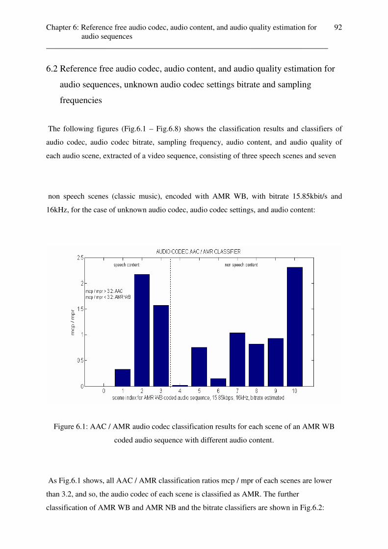
Chapter 6: Reference free audio codec, audio content, and audio quality estimation for audio sequences ________________________________________________________________________
92
6.2 Reference free audio codec, audio content, and audio quality estimation for
audio sequences, unknown audio codec settings bitrate and sampling
frequencies
The following figures (Fig.6.1 – Fig.6.8) shows the classification results and classifiers of
audio codec, audio codec bitrate, sampling frequency, audio content, and audio quality of
each audio scene, extracted of a video sequence, consisting of three speech scenes and seven
non speech scenes (classic music), encoded with AMR WB, with bitrate 15.85kbit/s and
16kHz, for the case of unknown audio codec, audio codec settings, and audio content:
Figure 6.1: AAC / AMR audio codec classification results for each scene of an AMR WB
coded audio sequence with different audio content.
As Fig.6.1 shows, all AAC / AMR classification ratios mcp / mpr of each scenes are lower
than 3.2, and so, the audio codec of each scene is classified as AMR. The further
classification of AMR WB and AMR NB and the bitrate classifiers are shown in Fig.6.2:
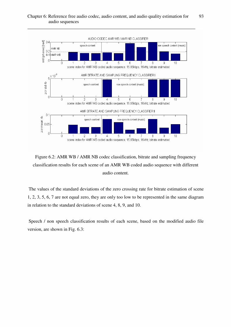
Chapter 6: Reference free audio codec, audio content, and audio quality estimation for audio sequences ________________________________________________________________________
93
Figure 6.2: AMR WB / AMR NB codec classification, bitrate and sampling frequency
classification results for each scene of an AMR WB coded audio sequence with different
audio content.
The values of the standard deviations of the zero crossing rate for bitrate estimation of scene
1, 2, 3, 5, 6, 7 are not equal zero, they are only too low to be represented in the same diagram
in relation to the standard deviations of scene 4, 8, 9, and 10.
Speech / non speech classification results of each scene, based on the modified audio file
version, are shown in Fig. 6.3:
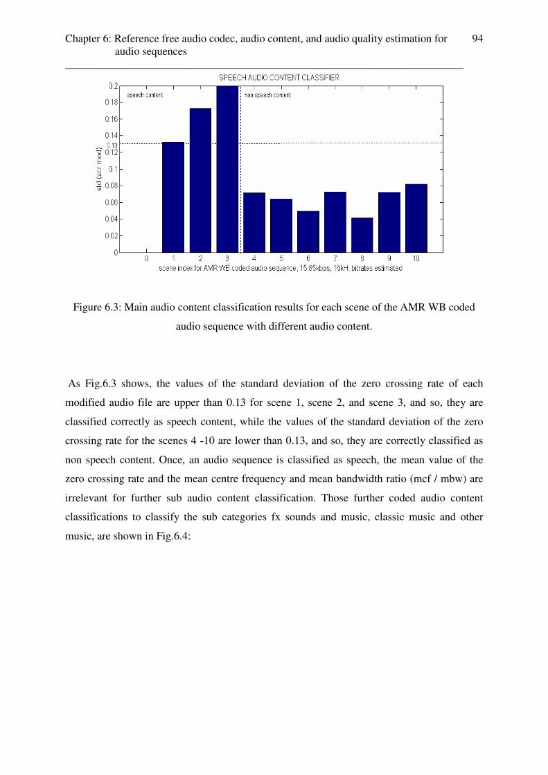
Chapter 6: Reference free audio codec, audio content, and audio quality estimation for audio sequences ________________________________________________________________________
94
Figure 6.3: Main audio content classification results for each scene of the AMR WB coded
audio sequence with different audio content.
As Fig.6.3 shows, the values of the standard deviation of the zero crossing rate of each
modified audio file are upper than 0.13 for scene 1, scene 2, and scene 3, and so, they are
classified correctly as speech content, while the values of the standard deviation of the zero
crossing rate for the scenes 4 -10 are lower than 0.13, and so, they are correctly classified as
non speech content. Once, an audio sequence is classified as speech, the mean value of the
zero crossing rate and the mean centre frequency and mean bandwidth ratio (mcf / mbw) are
irrelevant for further sub audio content classification. Those further coded audio content
classifications to classify the sub categories fx sounds and music, classic music and other
music, are shown in Fig.6.4:
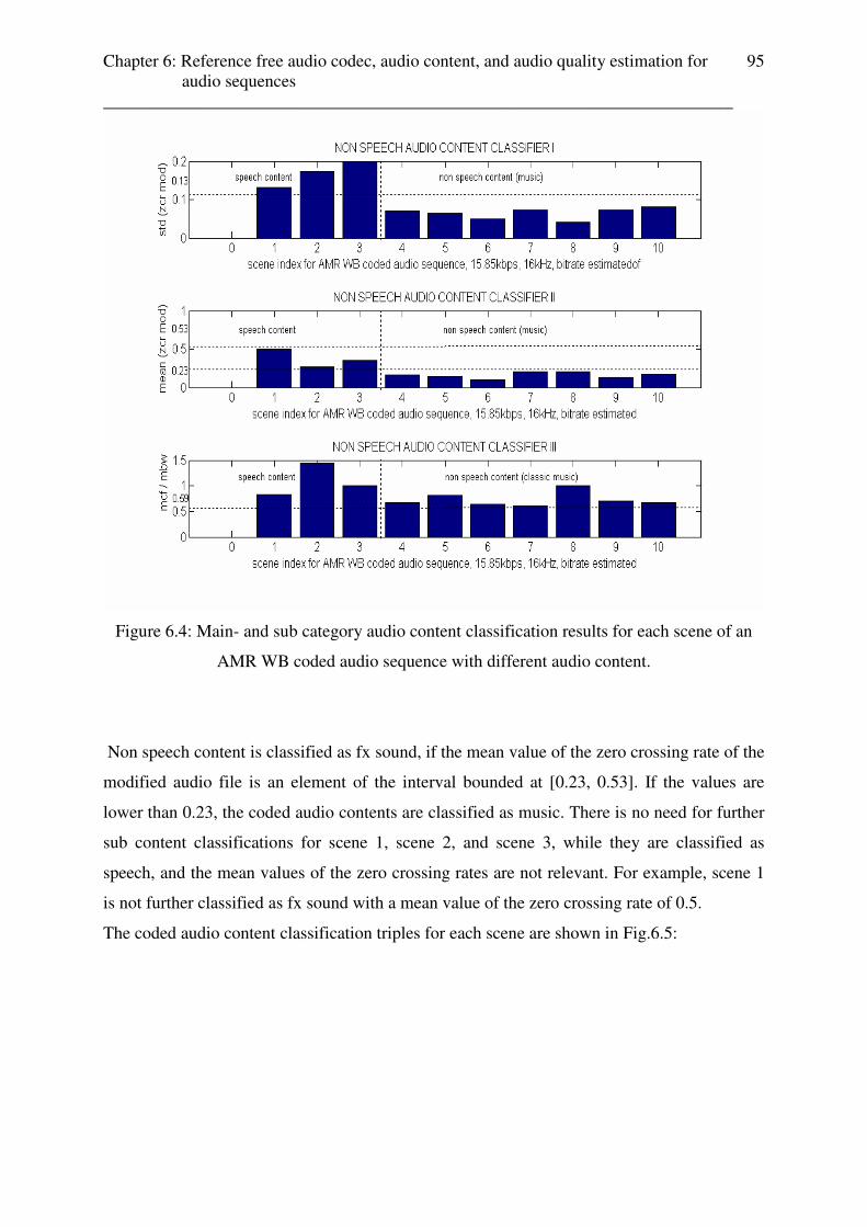
Chapter 6: Reference free audio codec, audio content, and audio quality estimation for audio sequences ________________________________________________________________________
95
Figure 6.4: Main- and sub category audio content classification results for each scene of an
AMR WB coded audio sequence with different audio content.
Non speech content is classified as fx sound, if the mean value of the zero crossing rate of the
modified audio file is an element of the interval bounded at [0.23, 0.53]. If the values are
lower than 0.23, the coded audio contents are classified as music. There is no need for further
sub content classifications for scene 1, scene 2, and scene 3, while they are classified as
speech, and the mean values of the zero crossing rates are not relevant. For example, scene 1
is not further classified as fx sound with a mean value of the zero crossing rate of 0.5.
The coded audio content classification triples for each scene are shown in Fig.6.5:

Chapter 6: Reference free audio codec, audio content, and audio quality estimation for audio sequences ________________________________________________________________________
96
Figure 6.5: Audio content classification results for each scene of the AMR WB coded audio
sequence with different audio content.
Once, a coded audio content is classified as speech, identified by a standard deviation value
of the zero crossing rate upper than 0.13, no further sub audio content classification is
necessary and the values of the two other classifiers (mean value of the zero crossing rate and
mcf / mbw ratio) are irrelevant: this can be seen in the results of the coded audio content
classification triple of scene 1, scene 2, scene 3. For all other scenes (scene 4 – scene 10), the
standard deviation of the zero crossing rates are lower than 0.13, they are classified as non
speech content, and so, the two other classifiers are relevant for further sub audio content
classification. While none of the fx sound classifiers (mean value of the zero crossing rate) for
scene 4 – scene 10 lies in the range of [0.23, 0.53], they are all classified as music. Further,
while all their mcf / mbw ratios are upper than 0.59, all scenes (4 – 10) are correctly classified
as classic music.
The relation between the audio quality parameter coefficient c, the estimated MOSApred, and
the rounded mean value of the MOS value from subjective tests, audio codec settings and
audio content specific, for each scene of the AMR WB coded audio sequence is shown in
Fig.6.7:
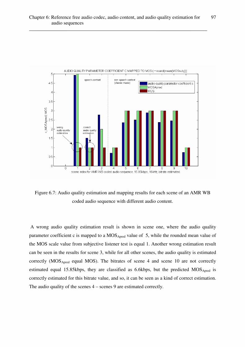
Chapter 6: Reference free audio codec, audio content, and audio quality estimation for audio sequences ________________________________________________________________________
97
Figure 6.7: Audio quality estimation and mapping results for each scene of an AMR WB
coded audio sequence with different audio content.
A wrong audio quality estimation result is shown in scene one, where the audio quality
parameter coefficient c is mapped to a MOSApred value of 5, while the rounded mean value of
the MOS scale value from subjective listener test is equal 1. Another wrong estimation result
can be seen in the results for scene 3, while for all other scenes, the audio quality is estimated
correctly (MOSApred equal MOS). The bitrates of scene 4 and scene 10 are not correctly
estimated equal 15.85kbps, they are classified as 6.6kbps, but the predicted MOSApred is
correctly estimated for this bitrate value, and so, it can be seen as a kind of correct estimation.
The audio quality of the scenes 4 – scenes 9 are estimated correctly.
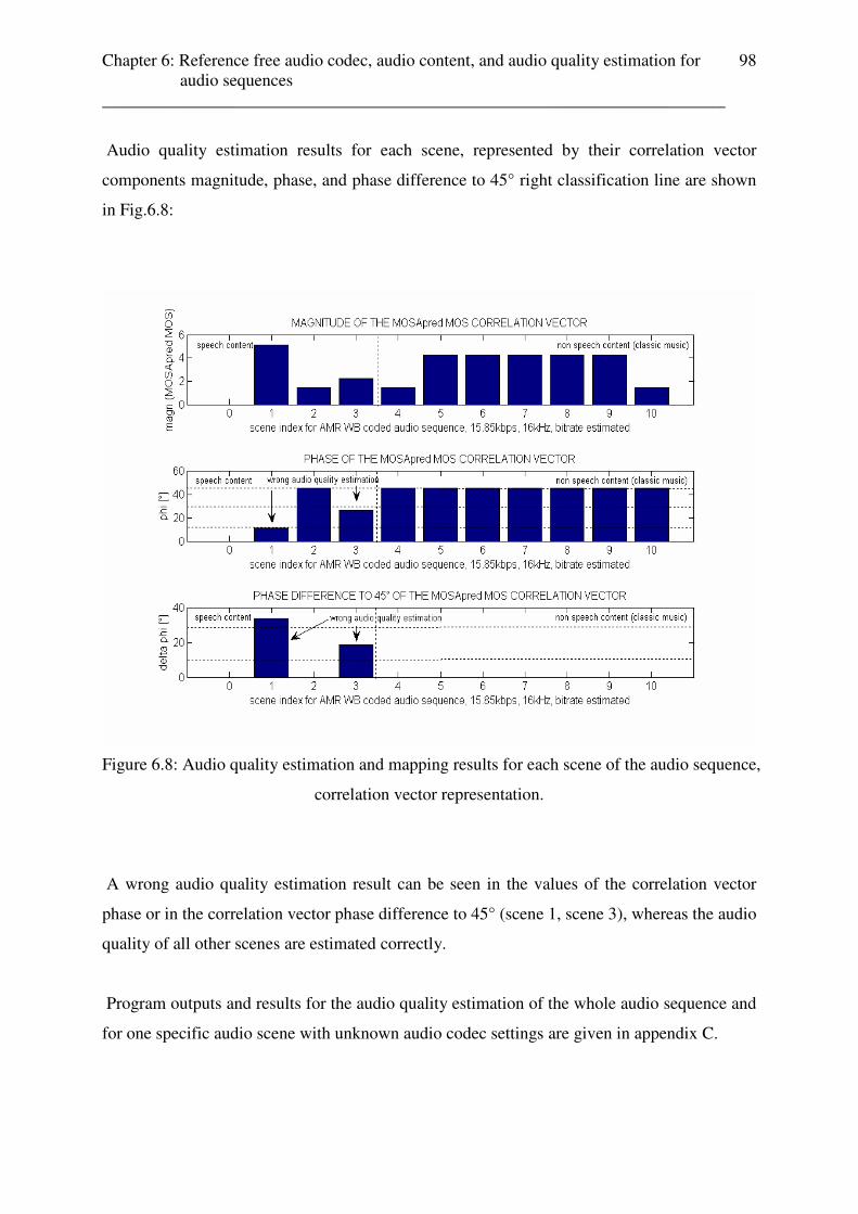
Chapter 6: Reference free audio codec, audio content, and audio quality estimation for audio sequences ________________________________________________________________________
98
Audio quality estimation results for each scene, represented by their correlation vector
components magnitude, phase, and phase difference to 45° right classification line are shown
in Fig.6.8:
Figure 6.8: Audio quality estimation and mapping results for each scene of the audio sequence,
correlation vector representation.
A wrong audio quality estimation result can be seen in the values of the correlation vector
phase or in the correlation vector phase difference to 45° (scene 1, scene 3), whereas the audio
quality of all other scenes are estimated correctly.
Program outputs and results for the audio quality estimation of the whole audio sequence and
for one specific audio scene with unknown audio codec settings are given in appendix C.
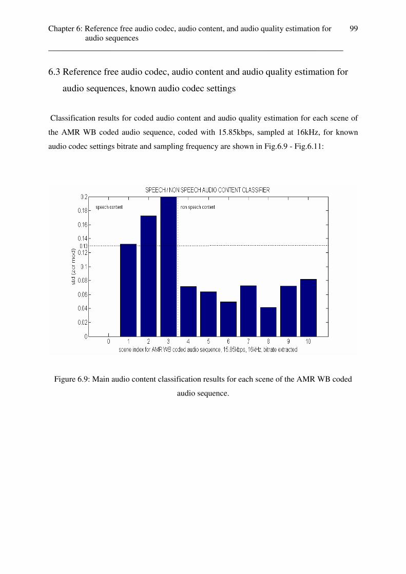
Chapter 6: Reference free audio codec, audio content, and audio quality estimation for audio sequences ________________________________________________________________________
99
6.3 Reference free audio codec, audio content and audio quality estimation for
audio sequences, known audio codec settings
Classification results for coded audio content and audio quality estimation for each scene of
the AMR WB coded audio sequence, coded with 15.85kbps, sampled at 16kHz, for known
audio codec settings bitrate and sampling frequency are shown in Fig.6.9 - Fig.6.11:
Figure 6.9: Main audio content classification results for each scene of the AMR WB coded
audio sequence.

Chapter 6: Reference free audio codec, audio content, and audio quality estimation for audio sequences ________________________________________________________________________
100
Figure 6.10: Main- and sub category audio content classification results for each scene of the
AMR WB coded audio sequence.
Figure 6.11: Audio content classification results for each scene of the AMR WB coded audio
sequence.
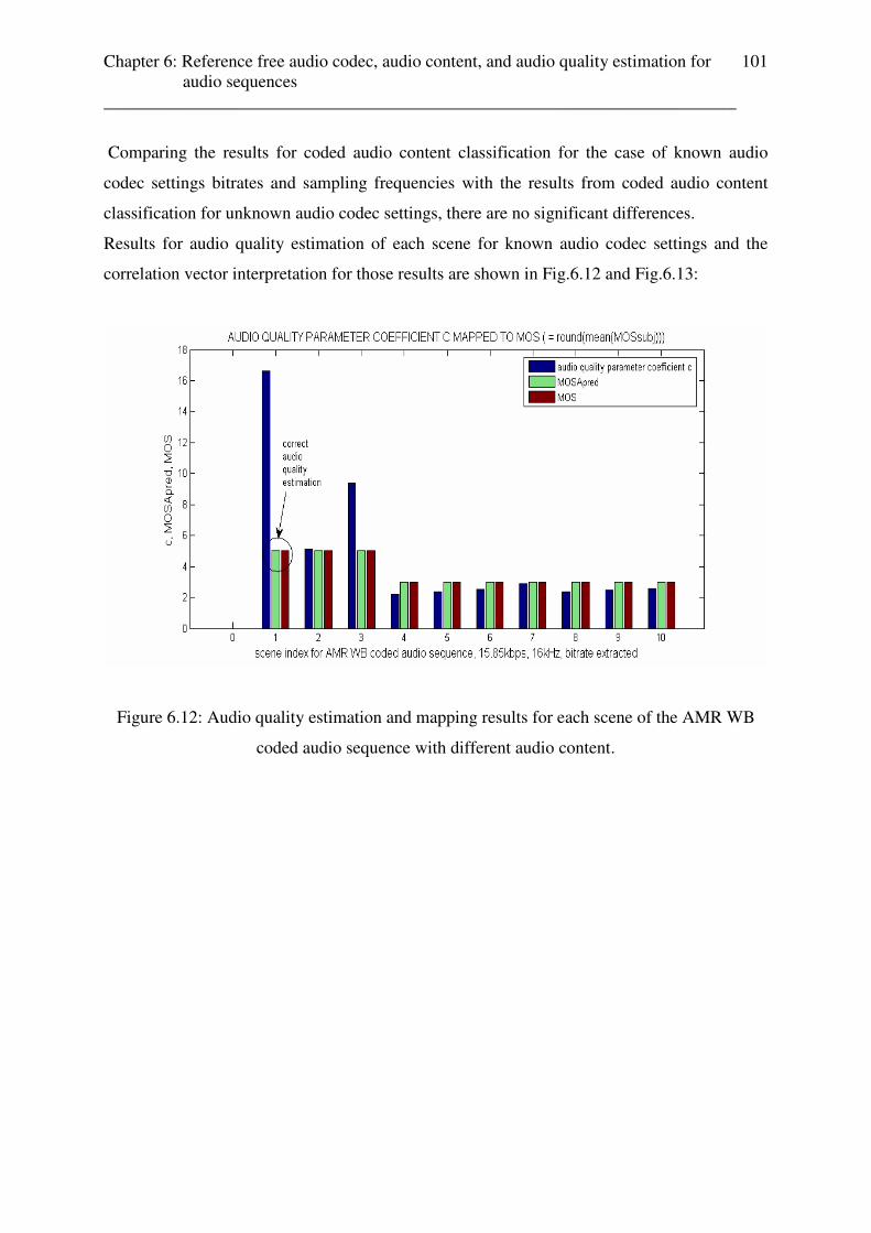
Chapter 6: Reference free audio codec, audio content, and audio quality estimation for audio sequences ________________________________________________________________________
101
Comparing the results for coded audio content classification for the case of known audio
codec settings bitrates and sampling frequencies with the results from coded audio content
classification for unknown audio codec settings, there are no significant differences.
Results for audio quality estimation of each scene for known audio codec settings and the
correlation vector interpretation for those results are shown in Fig.6.12 and Fig.6.13:
Figure 6.12: Audio quality estimation and mapping results for each scene of the AMR WB
coded audio sequence with different audio content.

Chapter 6: Reference free audio codec, audio content, and audio quality estimation for audio sequences ________________________________________________________________________
102
Figure 6.13: Audio quality estimation and mapping results for each scene of the audio
sequence, correlation vector representation.
Comparing this results with those of unknown audio codec settings, it can be seen, that for
the case of known audio codec settings the audio quality estimation for all scenes are correct,
even for scene 1 and scene 3. The audio quality of the first three AMR WB coded speech
scenes with15.85kbps, sampled at 16kHz is correctly estimated as “5 ... excellent”, and the
audio quality of the AMR WB coded classic music scenes with 15.85kbps, sampled at 16kHz
is correctly estimated as “3 ... fair”. Comparing both classification results from the audio
quality estimation for unknown and known audio codec setting characteristics, it can be seen,
that there are no significant differences in the classification and estimation results of each
stage of the whole audio quality estimation system.
Program outputs and results for the audio quality estimation of the whole audio sequence and
for one specific audio scene with known audio codec settings are given in appendix C.
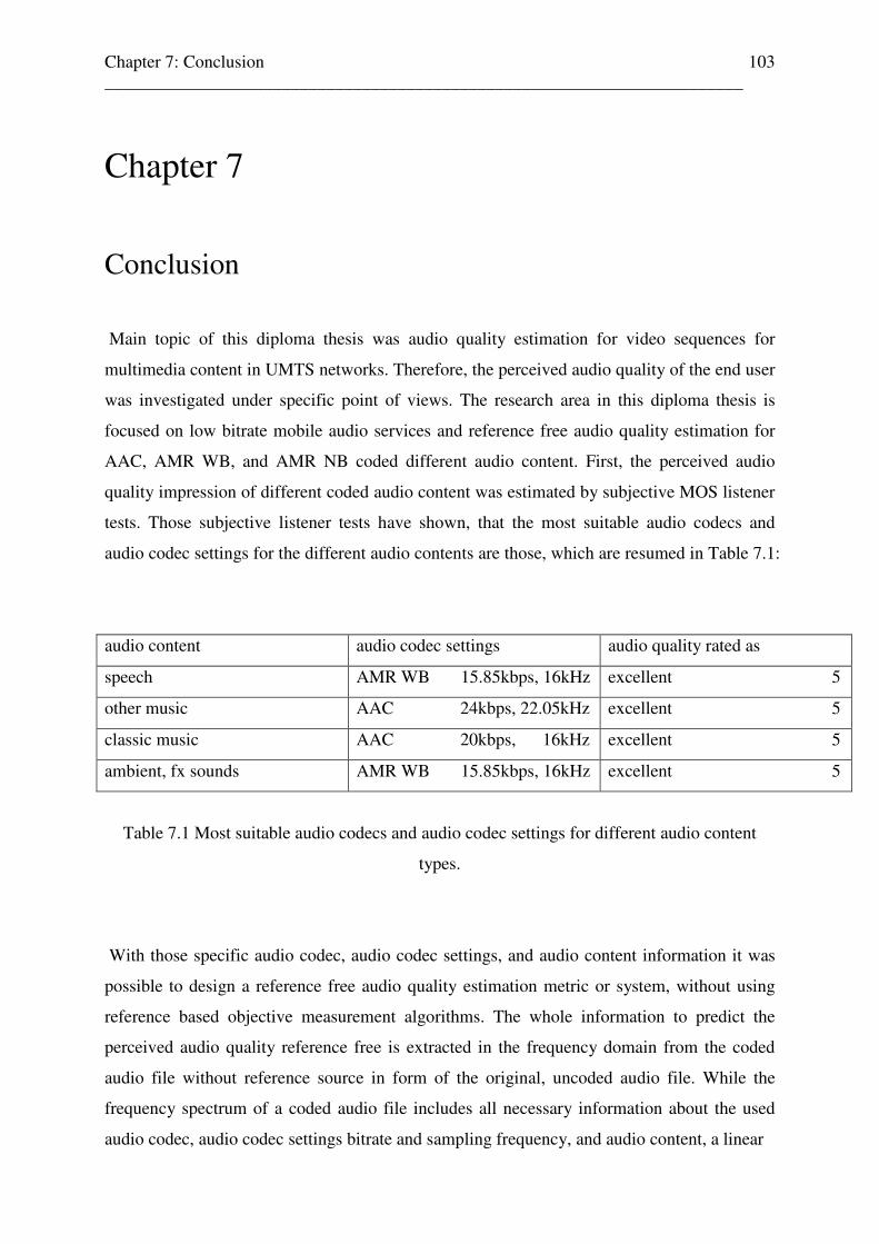
Chapter 7: Conclusion ________________________________________________________________________
103
Chapter 7
Conclusion
Main topic of this diploma thesis was audio quality estimation for video sequences for
multimedia content in UMTS networks. Therefore, the perceived audio quality of the end user
was investigated under specific point of views. The research area in this diploma thesis is
focused on low bitrate mobile audio services and reference free audio quality estimation for
AAC, AMR WB, and AMR NB coded different audio content. First, the perceived audio
quality impression of different coded audio content was estimated by subjective MOS listener
tests. Those subjective listener tests have shown, that the most suitable audio codecs and
audio codec settings for the different audio contents are those, which are resumed in Table 7.1:
audio content audio codec settings audio quality rated as
speech AMR WB 15.85kbps, 16kHz excellent 5
other music AAC 24kbps, 22.05kHz excellent 5
classic music AAC 20kbps, 16kHz excellent 5
ambient, fx sounds AMR WB 15.85kbps, 16kHz excellent 5
Table 7.1 Most suitable audio codecs and audio codec settings for different audio content
types.
With those specific audio codec, audio codec settings, and audio content information it was
possible to design a reference free audio quality estimation metric or system, without using
reference based objective measurement algorithms. The whole information to predict the
perceived audio quality reference free is extracted in the frequency domain from the coded
audio file without reference source in form of the original, uncoded audio file. While the
frequency spectrum of a coded audio file includes all necessary information about the used
audio codec, audio codec settings bitrate and sampling frequency, and audio content, a linear
Chapter 7: Conclusion ________________________________________________________________________
104
reference free audio quality estimation metric was designed together with the audio codec
and audio content specific results from the subjective MOS listener tests mean(MOSsubj). A
linear metric parameter p, proportional to the mean value of the audio codec and audio
content
specific subjective MOS listener test result, was found in the frequency domain in form of the
mean value of the magnitudes over all frames of a coded audio file frequency spectrum.
To predict the perceived audio quality by a reference free linear audio quality metric, it is
necessary to identify the audio codec, audio codec settings bitrate and sampling frequency,
and audio content by classification algorithms. Once, all of those audio file characteristics are
classified, the corresponding mean value from the subjective MOS listener tests result can be
chosen from a lookout table for estimating the perceived audio quality MOSApred in the
following way: first, the audio quality parameter coefficient c is calculated as the ratio of the
codec and content specific mean(MOSsubj) and the extracted audio quality parameter p, as
resumed in equation 7.1:
c = mean (MOSsubj) / p (7.1)
or
mean (MOSsubj) = c · p (7.2)
The predicted audio quality MOSApred is then calculated by mapping the specific audio
quality parameter coefficient c to the rounded version of the corresponding mean(MOSsubj)
value, as resumed in equation 7.3:
MOSApred = mapped( c ) = round (mean(MOSsubj)) (7.3)
or, c expressed in terms of mean(MOSsubj) and p:
MOSApred = mapped (mean(MOSsubj)/p) (7.4)

Chapter 7: Conclusion ________________________________________________________________________
105
As mentioned above, audio codec, audio codec settings, and audio content classifications are
necessary to identify the corresponding mean(MOSsubj) value for predicting the audio quality
MOSApred. Therefore, classifiers were found in the time- and frequency domain, such as:
- the mean centre phase mean phase range ratio for AAC / AMR codec classification
- the standard deviation of the phase for AMR WB / AMR NB classification
- the mean centre phase for AAC bitrate and sampling frequency classification
- the standard deviation and mean value combination of the zero crossing rate for AMR
WB and AMR NB bitrate and sampling frequency classification
- the standard deviation of the zero crossing rate of a modified coded audio file version
for speech / non speech content classification
- the mean value of the zero crossing rate of a modified coded audio file version for
fx sounds / music classification
- the mean centre frequency and mean bandwidth ratio for classic music and other
music classification
All of this classifier and their threshold values are resumed in Table 7.2:
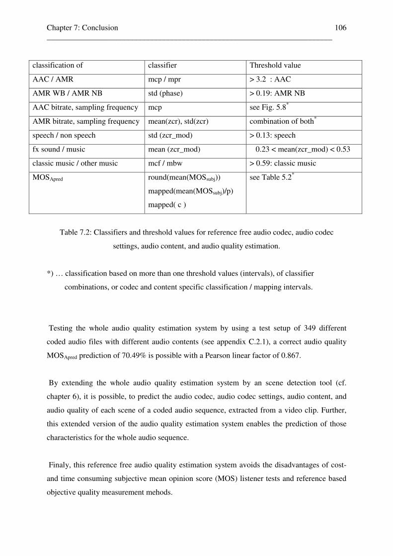
Chapter 7: Conclusion ________________________________________________________________________
106
classification of classifier Threshold value
AAC / AMR mcp / mpr > 3.2 : AAC
AMR WB / AMR NB std (phase) > 0.19: AMR NB
AAC bitrate, sampling frequency mcp see Fig. 5.8*
AMR bitrate, sampling frequency mean(zcr), std(zcr) combination of both*
speech / non speech std (zcr_mod) > 0.13: speech
fx sound / music mean (zcr_mod) 0.23 < mean(zcr_mod) < 0.53
classic music / other music mcf / mbw > 0.59: classic music
MOSApred round(mean(MOSsubj))
mapped(mean(MOSsubj)/p)
mapped( c )
see Table 5.2*
Table 7.2: Classifiers and threshold values for reference free audio codec, audio codec
settings, audio content, and audio quality estimation.
*) … classification based on more than one threshold values (intervals), of classifier
combinations, or codec and content specific classification / mapping intervals.
Testing the whole audio quality estimation system by using a test setup of 349 different
coded audio files with different audio contents (see appendix C.2.1), a correct audio quality
MOSApred prediction of 70.49% is possible with a Pearson linear factor of 0.867.
By extending the whole audio quality estimation system by an scene detection tool (cf.
chapter 6), it is possible, to predict the audio codec, audio codec settings, audio content, and
audio quality of each scene of a coded audio sequence, extracted from a video clip. Further,
this extended version of the audio quality estimation system enables the prediction of those
characteristics for the whole audio sequence.
Finaly, this reference free audio quality estimation system avoids the disadvantages of cost-
and time consuming subjective mean opinion score (MOS) listener tests and reference based
objective quality measurement mehods.
Appendix A: Multimedia streaming in UMTS networks ________________________________________________________________________
107
Appendix A
Multimedia streaming in UMTS networks
A.1 Introduction
Streaming is a method for transferring data with real-time characteristics [32], so that the user
(recipient) can start viewing the presentation before the entire contents have been transmitted.
A streaming platform supports a multitude of different multimedia applications and contents,
at various bitrates and qualities. For example, news at very low bitrates using still images and
speech, music listenings, video clips and watching live sports events. Such streaming
platforms are supporting also progressive downloading of media for selective media types,
which can be further protected with a standardised digital rights management (DRM)
technology.
During the streaming process, a server sends multimedia content to an user (client or
recipient) over a network in real-time. In a transparent end-to-end packet switched streaming
service (PSS), the multimedia content is divided into packets by the streaming server to make
a transmission over the network possible. Such a transparent end-to-end packet-switched
streaming service PSS is specified by the third generation partnership project (3GPP) in which
multimedia streaming packets are reassembled by the user at the receivers end, which enables
the user to play the multimedia content as it comes in. A series of related packets is called a
stream. The data packets are sent in real time and time-stamped, so they can be displayed in
time-synchronized order. There are two possibilities to transmit such real time strings: unicast
or multicast. In the case of unicast, the real time streams are sent from one server to one client
(one-to-one), and in the case of multi cast, the real time streams are sent from one server to
more than one client (one-to-many). The main difference from simple file transfer and
streaming lies in the fact, that the client can play the multimedia content as it comes in over
the network, rather than waiting for the entire multimedia content to download before it can
be played. For streaming, the multimedia service must be able to relate media components to
each other. For example, in a multimedia stream, consisting of video- and audio content, both
components must be synchronized. Section 2.2-2.4 gives an overview over the architecture,

Appendix A: Multimedia streaming in UMTS networks ________________________________________________________________________
108
streaming mechanism, streaming codecs, file formats, streaming protocols, and network
elements involved in a transparent end-to-end packet switched streaming service (PSS).
A.2 Transparent end-to-end packet switched streaming service (PSS)
Transparent end-to-end packet switched streaming service (PSS) is a specification by the
third generation partnership project (3GPP), which is a collaboration agreement between
several telecommunication standardization bodies [34]. PSS defines a framework for an
interoperable streaming service in 3GPP mobile networks and is an application level service
that mostly deals with client and server. Although streaming can benefit from network support
(e.g. Quality of Service QoS), one requirement for PSS is that it should work over different
(QoS) bearers. Therefore, multimedia services should be designed in such a way that they can
be adapted to the network.
The basic framework appeared the first time by simple streaming services in Release 4 of the
3GPP specification. 3GPP Release 5 had introduced extended features such as capability
exchange while the backward compatible 3GPP Release 6 completes the PSS feature set to a
comprehensive content delivery framework. 3GPP release 6 framework updates the list of
recommended media types and codecs to achive higher service quality within the 3GPP
environments. An overview of network elements involved in a 3G packet switched streaming
service are presented in Fig.A.1 [33]:
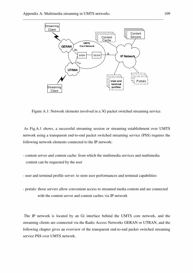
Appendix A: Multimedia streaming in UMTS networks ________________________________________________________________________
109
Streaming
Client
ContentServers
User and
terminalprofiles
Portals
IP Network
Content Cache
UMTS
Core Network
UTRAN
GERAN
SGSN GGSNGi
Gb
Iups
Streaming
Client
Figure A.1: Network elements involved in a 3G packet switched streaming service.
As Fig.A.1 shows, a successful streaming session or streaming establishment over UMTS
network using a transparent end-to-end packet switched streaming service (PSS) requires the
following network elements connected to the IP network:
- content server and content cache: from which the multimedia services and multimedia
content can be requested by the user
- user and terminal profile server: to store user performances and terminal capabilities
- portals: those servers allow convenient access to streamed media content and are connected
with the content server and content caches via IP network
The IP network is located by an Gi interface behind the UMTS core network, and the
streaming clients are connected via the Radio Access Networks GERAN or UTRAN, and the
following chapter gives an overview of the transparent end-to-end packet switched streaming
service PSS over UMTS network.
Appendix A: Multimedia streaming in UMTS networks ________________________________________________________________________
110
A.3 Streaming scenario in UMTS
A simple streaming session in a packet switched streaming application (PSS) consists of
streaming control protocols, transport protocols, media codecs, and scene description
protocols. At the beginning of every streaming session, the mobile user gets an universal
resource identifier (URI), specifying a streaming server and the content address on that server.
There are three possibilities how a mobile user can get an URI: from a world wide web
(WWW) browser, from a wireless application protocol (WAP) browser, or typed by hand.
The description of a streaming session in relation to the requested content characteristics
(session name, author, ...), media type, and transmission bitrate is given in the Session
Description Protocol (SDP) file. This SDP file can be given in the link of a HTML page,
through a Real-Time Streaming Protocol (RTSP) [35], or via a Multimedia Session Service
(MMS). Here, the MMS user agent receives a modified MMS message from the MMS relay
or server.
Every streaming session starts with the so called session establishment, a process, in which
the browser or the mobile user invokes a streaming client to set up the session against the
server. An active PDP context in accordance with [40] or other type of radio bearer that
enables IP packet transmission is expected from the UE at the start of the session
establishment signalling. The client may be able to ask for more information about the content
and shall initiate the provisioning of a bearer with appropriate QoS for the streaming media.
The basic RTSP unicast operation first appeared in 3GPP Release 4, in which the client or
mobile user gets an universal resource identifier (URI), which specifies a streaming server
and the address of the content on that server, from a WWW-browser or WAP-browser, or
learns the location of a media clip by browsing to a web page that has an RTSP URI. The
streaming player connects to the streaming server and issues a RTSP DESCRIBE command.
The server responds with an Session Description Protocol (SDP) which includes information
like number of streams, media types, and required bandwidth. After parsing the description,
the client issues an RTSP SETUP command for each stream in the session. The SETUP
command tells the server which ports the client uses to receive the media. When streams have
been set up, the client issues a RTSP PLAY command after which the server starts sending
one or more media streams as RTP packets over the IP network. Finally, the client issues a

Appendix A: Multimedia streaming in UMTS networks ________________________________________________________________________
111
TEARDOWN command to end the streaming session. This schematic view of a streaming
session is illustrated in [33].
In 3GPP Release 5, during the streaming initiation, the client provides a capability profile to
the server (an URL reffering to the profle and possible differences) [33]. With the PSS
capability profile, the client can send information about its available number of audio
channels, supported media types, rendering screen size, and bits per pixel to the server, which
further uses this information to select the most suitable content for the client.
3GPP Release 6 consists of already defined download and streaming framework appended
with alternative of progressive downloading in an end-to-end delivery context. This enables
optional use of strong content encryption and integrity protection capabilities and
interoperability with cryptographic key management systems.
Between PSS providers a standardised container file exchange is possible as a specific server
file format. For session bandwidth adaption to the potentially time-varying cellular network
bandwidth, PSS allows the selection of streaming session alternatives (alternative SDP) and
dynamic, link-aware bandwidth adaptation. This feature is especially useful in cellular
networks where QoS-enabled bearers are not available. 3GPP Release 6 also presents a
defined mechanism to gather streaming session Quality-of-Experience metrics at the PSS
service provider’s premises. The capability exchange mechanisms in Release 6 enable better
service filtering for both streaming and static media contents. Further, a progressive
downloading mechanism is implemented in Release 6 to start media playback during the
media “download”. The 3GPP PSS provides a framework for Internet Protocol (IP) based
streaming applications in 3G networks.
A.3.1 Streaming protocols in UMTS
Streaming Protocols are essential for PSS to control session establishment, session-setup,
capability exchange, session control, scene description, and data transport of streaming media
and other data. The following streaming related protocols utilize TCP / IP [38] and / or UDP /
IP [39] as their transport [32]:
Appendix A: Multimedia streaming in UMTS networks ________________________________________________________________________
112
- RTP: Real-Time Transport Protocol [RFC 1889, RFC 1890]
Provides end-to-end network transport functions suitable for applications
transmitting real-time data, such as audio or video, over multicast or unicast
network services. In PSS, RTP is carried only over UDP and does not
guarantee quality-of-service for real-time services,
- RTCP: Real-Time Control Protocol [RFC 1889]
The primary function of RTCP is to provide feedback on the quality of data
distribution, which is achieved by periodic “receiver report” packets sent by
the receiver to the sender, containing inter-arrival jitter measured by the
receiver and number of packets lost [35];
- RTSP: Real-Time Streaming Protocol [RFC 2326]
RTSP is used to establish and control time-symchronized streams of continous
media and acts as a “network remote control” for multimedia services;
- SDP: Session Description Protocol [RFC 2327, RFC 2326]
The purpose of SDP is to convey information about media streams in
multimedia sessions to allow the recipients of a session description to
participate in the session,
- UDP/IP: User datagram protocol [RFC 768]
for transport of RTP flows and data,
- TCP/IP: Transmission control protocol [RFC 793]:
for transport of data only,
- SCTP/IP: Stream control transmission protocol [RFC 3286]
IP media transport protocol that also provides telephony signaling
transport critical functions.
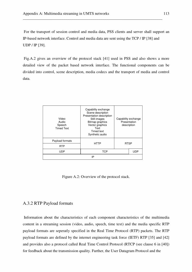
Appendix A: Multimedia streaming in UMTS networks ________________________________________________________________________
113
For the transport of session control and media data, PSS clients and server shall support an
IP-based network interface. Control and media data are sent using the TCP / IP [38] and
UDP / IP [39].
Fig.A.2 gives an overview of the protocol stack [41] used in PSS and also shows a more
detailed view of the packet based network interface. The functional components can be
divided into control, scene description, media codecs and the transport of media and control
data.
IP
UDP TCP
RTP RTSP
Payload formats
Video Audio
Speech
Capability exchange Scene description
Presentation description Still images
Bitmap graphics Vector graphics
Text Timed text
Synt hetic audio
HTTP
Capability exchange Presentation description
UDP
Timed Text
Figure A.2: Overview of the protocol stack.
A.3.2 RTP Payload formats
Information about the characteristics of each component characteristics of the multimedia
content in a streaming session (video, audio, speech, time text) and the media specific RTP
payload formats are seperatly specified in the Real Time Protocol (RTP) packets. The RTP
payload formats are defined by the internet engineering task force (IETF) RTP [35] and [42]
and provides also a protocol called Real Time Control Protocol (RTCP (see clause 6 in [40])
for feedback about the transmission quality. Further, the User Datagram Protocol and the
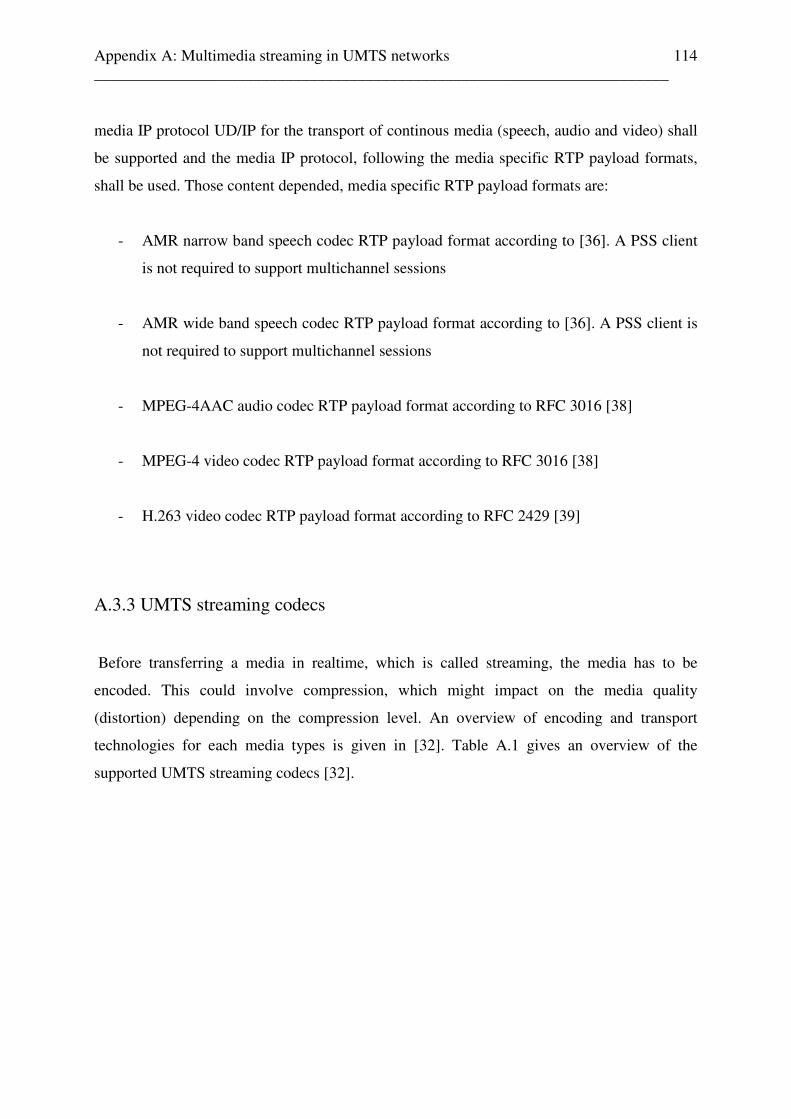
Appendix A: Multimedia streaming in UMTS networks ________________________________________________________________________
114
media IP protocol UD/IP for the transport of continous media (speech, audio and video) shall
be supported and the media IP protocol, following the media specific RTP payload formats,
shall be used. Those content depended, media specific RTP payload formats are:
- AMR narrow band speech codec RTP payload format according to [36]. A PSS client
is not required to support multichannel sessions
- AMR wide band speech codec RTP payload format according to [36]. A PSS client is
not required to support multichannel sessions
- MPEG-4AAC audio codec RTP payload format according to RFC 3016 [38]
- MPEG-4 video codec RTP payload format according to RFC 3016 [38]
- H.263 video codec RTP payload format according to RFC 2429 [39]
A.3.3 UMTS streaming codecs
Before transferring a media in realtime, which is called streaming, the media has to be
encoded. This could involve compression, which might impact on the media quality
(distortion) depending on the compression level. An overview of encoding and transport
technologies for each media types is given in [32]. Table A.1 gives an overview of the
supported UMTS streaming codecs [32].
Appendix A: Multimedia streaming in UMTS networks ________________________________________________________________________
115
Type Codec
(Decoder)
Support Max. Bitrate
[kbps]
Notes
Speech AMR-NB Required 12.2
Speech AMR-WB Required 23.85
Audio MPEG-4 AAC-
LC
Recommended N/A
Audio MPEG-4 AAC-
LTP
Optional N/A
Video H.263 profile 0
level 10
Required 64 Max. Frame size
176x144
Video H.263 profile 3
level 10
Recommended 64 Interactive and
wireless
streaming
profile.
Video MPEG-4 Simple
Visual Profile
Level 0
Recommended 64 Max. Frame size
176x144
Table A.1: 3GPP PSS audio and video codecs [32].
A.3.4 UMTS streaming file formats
While the streaming coding format is used to transform the multimedia content into a code
stream, the specific streaming file format enables the prestored code stream for local decoding
and playback, for the transfer on different media, or for different streaming transport.
UMTS streaming supports .3gp and .mp4 streaming formats [34]. The .3gp file format is
defined by 3GPP [34] as a standard for multimedia streaming services over wireless networks
and is based on ISO base file format [34], which allows the mixing and seperation of different
media types. Table 2 gives an overview over the conformance of .3gp and .mp4 streaming file

Appendix A: Multimedia streaming in UMTS networks ________________________________________________________________________
116
formats to one or more several user or client profiles and examples for brands in 3GP files [34]
are given in Table A.2:
Conformance
Suffix
Brand Compatible brands Example content
Streaming servers: Some files may in principle also be used for MMS or download.
Release 6 .3gp 3gs6 3gs6, isom AMR and hint track
Release 6 .3gp 3gs6 3gs6, isom 2 tracks H.263 and 2 hint tracks
Release 6, 5, 4 .3gp 3gs6 3gs6, 3gp6, 3gp5, 3gp4,
isom
H.263, AMR and hint tracks
3GP file, also conforming to MP4
Release 4, 5 and
MP4
.3gp 3gp5 3gp5, 3gp4, mp42, isom MPEG-4 video
MP4 file, also conforming to 3GP
Release 5 and MP4 .mp4 mp42 Mp42, 3gp5, isom MPEG-4 video and AAC
Table A.2: Conformance of different streaming file formats in UMTS [34].
A brand identifies a specification or a conformance point in a specification; its presence in a
file indicates :
- that the file conforms to the specification;
- that a reader implementing that specification is given permission to read and interpret
the file.
For example, the brand ‘isom’ indicates conformance to the base structure of the ISO base
media file format [32]. The 3GP General profile is branded ‘3gg6’ while the 3GP Basic
profile is branded ‘3gp6’ and used in MMS and PSS.

Appendix A: Multimedia streaming in UMTS networks ________________________________________________________________________
117
A.4 Mobile Multimedia services
3G mobile networks are characterized by their ability to carry data at much higher rates than
the generations of mobile networks before (i.e., 9.6 kbps). It allows a 384 kbps packet-
switched connection for downlink and 62 kbps circuit switch connection that is N-ISDN
compatible. The 3G mobile networks provide significant greater bandwidth and is so suitable
for new mobile services, such as enhanced multimedia applications and services A service can
be classified as multimedia when it involves at least two of the following media types [43]:
- Speech: voice telecommunication (300-3400 Hz), focusing on mouth-to-ear intelligibility
- Audio: telecommunication of sound in general, focusing on fidelity. Various quality levels
can be provided, high fidelity implying complete audio frequency spectrum (20-
20000 Hz) and 44.1 kHz sampling.
- Video: telecommunication of full motion pictures and stills, focusing on fidelity.
- Data: telecommunication of information files (text, graphics, data), focusing on error-free
transfer.
Applications, which can be built on top of streaming services, can be classified into on-
demand and live information delivery applications. Examples of the first category are music
and news-on-demand applications. Live delivery of radio and television programs are
examples of the second category. Further, the multimedia service must be able to relate
synchronized multimedia components, such as audio and video.
A.5 Quality of Service in UMTS network
The perception of an user about a delivered service, including multimedia applications and
multimedia contents, can be identified with the quality of the service QoS. A number of
parameters can influence this user perception, and the influencing parameters can differ as a
function of the service, applications, or contents. Several studies have shown, that the main

Appendix A: Multimedia streaming in UMTS networks ________________________________________________________________________
118
parameters influencing the QoS perception of a transparent end-to-end packet switched
streaming service (PSS) are [37]:
- Guaranteed bandwidth
- Delay
- Jitter
- Packet loss
All of those parameter influences the perceptual quality of a service and also the perceptual
quality of the service content. For example, delays and packet loss during a streaming session
leads to a low user quality perception. The available bandwidth enables the usage of different
multimedia codecs with different codec settings to receive best possible user perception and
satisfaction. Therefore, the quality of the choosen multimedia codec with its technical
characteristics and codec settings within a service, can be reflected by a “mean opinion score”
(MOS), assigned to the specific codec. So, the perceived QoS can be determed for the whole
service, or especially for the multimedia codecs within the delivered service. A special
method of specifying and grouping applications into QoS categories to indicate the
importance of the different parameters as functions of the delivered service (QoS indicators)
is the Class of Service CoS concept, which is defined in [37]. The end-to-end QoS concept
and architecture for UMTS up to IP layer is defined in [37] and Table A.3 gives an overview
of QoS classes in UMTS:
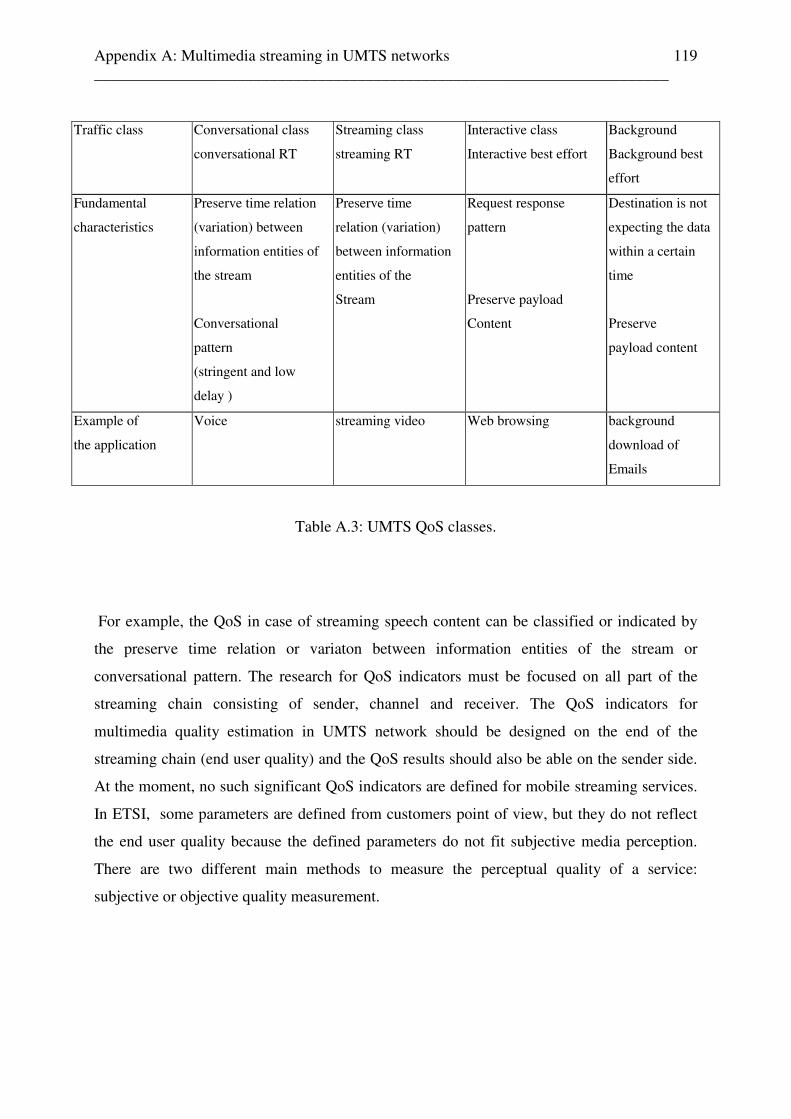
Appendix A: Multimedia streaming in UMTS networks ________________________________________________________________________
119
Traffic class Conversational class
conversational RT
Streaming class
streaming RT
Interactive class
Interactive best effort
Background
Background best
effort
Fundamental
characteristics
Preserve time relation
(variation) between
information entities of
the stream
Conversational
pattern
(stringent and low
delay )
Preserve time
relation (variation)
between information
entities of the
Stream
Request response
pattern
Preserve payload
Content
Destination is not
expecting the data
within a certain
time
Preserve
payload content
Example of
the application
Voice streaming video Web browsing background
download of
Emails
Table A.3: UMTS QoS classes.
For example, the QoS in case of streaming speech content can be classified or indicated by
the preserve time relation or variaton between information entities of the stream or
conversational pattern. The research for QoS indicators must be focused on all part of the
streaming chain consisting of sender, channel and receiver. The QoS indicators for
multimedia quality estimation in UMTS network should be designed on the end of the
streaming chain (end user quality) and the QoS results should also be able on the sender side.
At the moment, no such significant QoS indicators are defined for mobile streaming services.
In ETSI, some parameters are defined from customers point of view, but they do not reflect
the end user quality because the defined parameters do not fit subjective media perception.
There are two different main methods to measure the perceptual quality of a service:
subjective or objective quality measurement.

Appendix B: Audio coding technologies ________________________________________________________________________
120
Appendix B
Audio coding technologies
The quality of wireless multimedia communication and services, is always limited by the
given bandwidth and the choosen multimedia codec characteristics. In relation to the existing
bandwidth gap between wireless and wired networks (one or two orders in their magnitude
[44]), it is important to have codecs that provide better coding efficiency and coding
technologies which achieved compact representations of media data over wireless networks.
This is done by data compression algorithms before the multimedia content is transfered in
realtime (streaming). Data compression allows the reduction of irrelevant information of the
source signal and influences always the quality of the multimedia content (distortions),
depending on the compression level. Current coding technologies were designed to minimize
further implementation and memory costs by this way [44]. An overview of the different
speech, audio and video codecs in relation to the bitrate and their applications are given in
Fig.B.1:
300k Bitrate [bit/s] MPEG-2 AAC 5.1 ch 100k MPEG-2 AAC ITU AMR codecs WB MPEG-4 High Effiency AAC 10k Audio quality Speech Wideband Stereo / HiFi Multi-channel speech audio Surrounding Audio
Figure B.1: Speech and audio codecs with regard to bitrate [44].
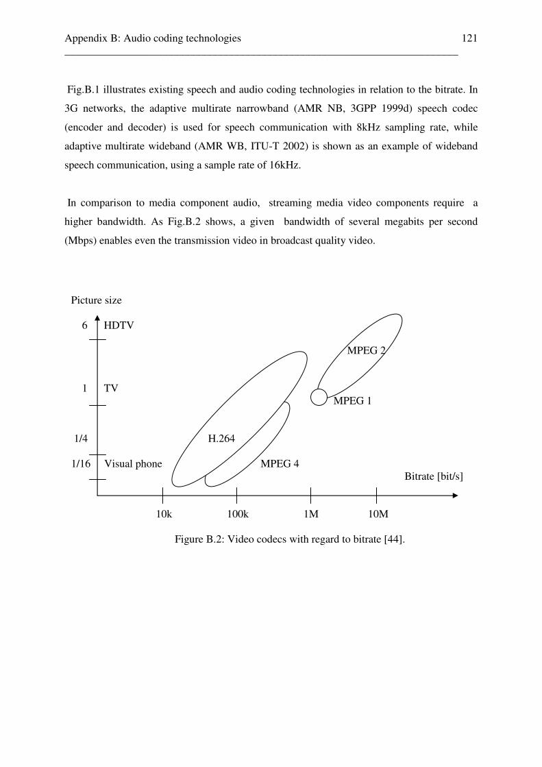
Appendix B: Audio coding technologies ________________________________________________________________________
121
Fig.B.1 illustrates existing speech and audio coding technologies in relation to the bitrate. In
3G networks, the adaptive multirate narrowband (AMR NB, 3GPP 1999d) speech codec
(encoder and decoder) is used for speech communication with 8kHz sampling rate, while
adaptive multirate wideband (AMR WB, ITU-T 2002) is shown as an example of wideband
speech communication, using a sample rate of 16kHz.
In comparison to media component audio, streaming media video components require a
higher bandwidth. As Fig.B.2 shows, a given bandwidth of several megabits per second
(Mbps) enables even the transmission video in broadcast quality video.
Picture size 6 HDTV MPEG 2 1 TV MPEG 1 1/4 H.264 1/16 Visual phone MPEG 4 Bitrate [bit/s] 10k 100k 1M 10M
Figure B.2: Video codecs with regard to bitrate [44].
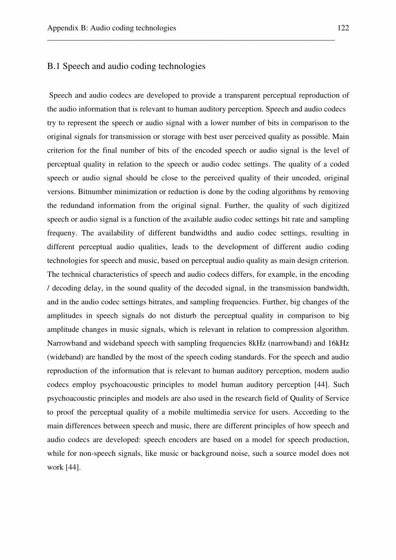
Appendix B: Audio coding technologies ________________________________________________________________________
122
B.1 Speech and audio coding technologies
Speech and audio codecs are developed to provide a transparent perceptual reproduction of
the audio information that is relevant to human auditory perception. Speech and audio codecs
try to represent the speech or audio signal with a lower number of bits in comparison to the
original signals for transmission or storage with best user perceived quality as possible. Main
criterion for the final number of bits of the encoded speech or audio signal is the level of
perceptual quality in relation to the speech or audio codec settings. The quality of a coded
speech or audio signal should be close to the perceived quality of their uncoded, original
versions. Bitnumber minimization or reduction is done by the coding algorithms by removing
the redundand information from the original signal. Further, the quality of such digitized
speech or audio signal is a function of the available audio codec settings bit rate and sampling
frequeny. The availability of different bandwidths and audio codec settings, resulting in
different perceptual audio qualities, leads to the development of different audio coding
technologies for speech and music, based on perceptual audio quality as main design criterion.
The technical characteristics of speech and audio codecs differs, for example, in the encoding
/ decoding delay, in the sound quality of the decoded signal, in the transmission bandwidth,
and in the audio codec settings bitrates, and sampling frequencies. Further, big changes of the
amplitudes in speech signals do not disturb the perceptual quality in comparison to big
amplitude changes in music signals, which is relevant in relation to compression algorithm.
Narrowband and wideband speech with sampling frequencies 8kHz (narrowband) and 16kHz
(wideband) are handled by the most of the speech coding standards. For the speech and audio
reproduction of the information that is relevant to human auditory perception, modern audio
codecs employ psychoacoustic principles to model human auditory perception [44]. Such
psychoacoustic principles and models are also used in the research field of Quality of Service
to proof the perceptual quality of a mobile multimedia service for users. According to the
main differences between speech and music, there are different principles of how speech and
audio codecs are developed: speech encoders are based on a model for speech production,
while for non-speech signals, like music or background noise, such a source model does not
work [44].
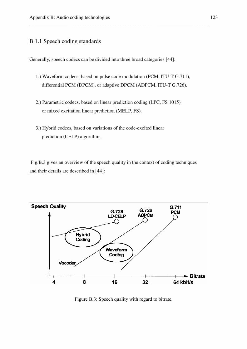
Appendix B: Audio coding technologies ________________________________________________________________________
123
B.1.1 Speech coding standards
Generally, speech codecs can be divided into three broad categories [44]:
1.) Waveform codecs, based on pulse code modulation (PCM, ITU-T G.711),
differential PCM (DPCM), or adaptive DPCM (ADPCM, ITU-T G.726).
2.) Parametric codecs, based on linear prediction coding (LPC, FS 1015)
or mixed excitation linear prediction (MELP, FS).
3.) Hybrid codecs, based on variations of the code-excited linear
prediction (CELP) algorithm.
Fig.B.3 gives an overview of the speech quality in the context of coding techniques
and their details are described in [44]:
Figure B.3: Speech quality with regard to bitrate.
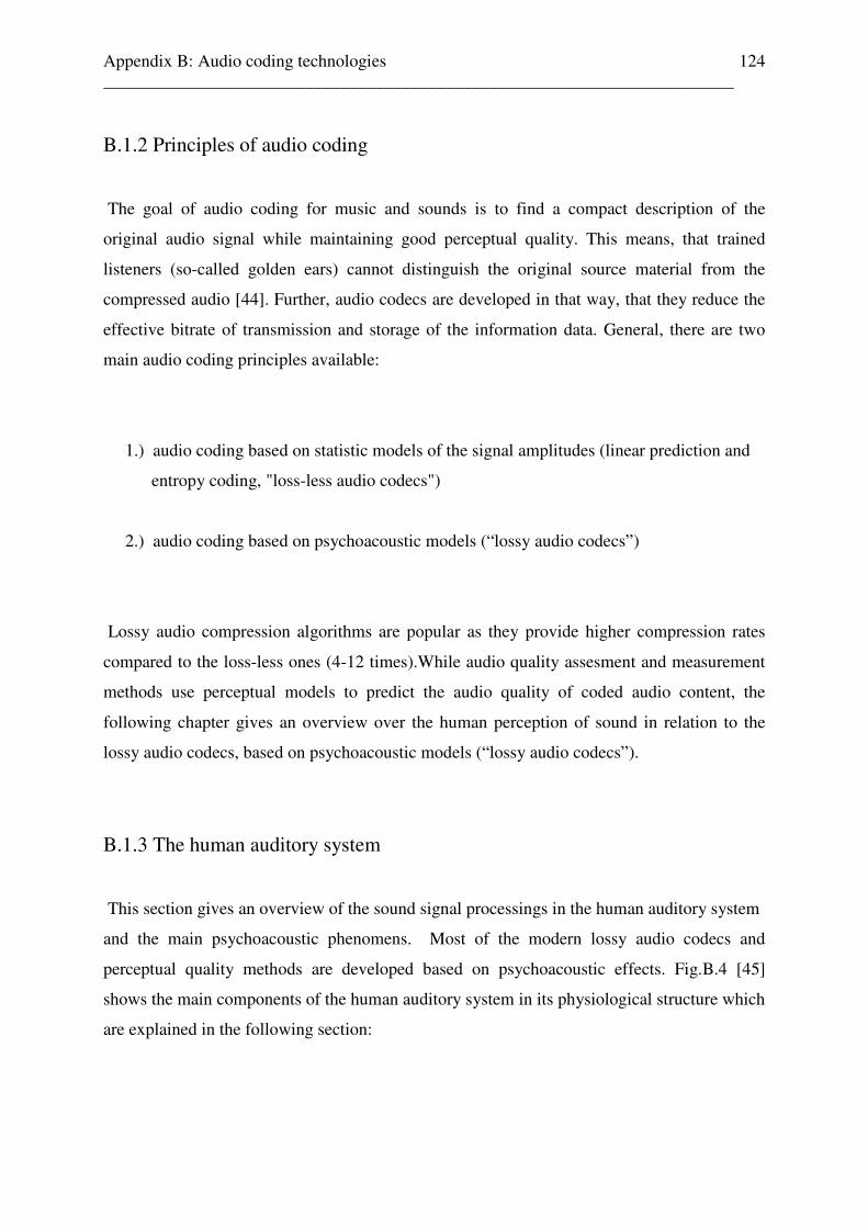
Appendix B: Audio coding technologies ________________________________________________________________________
124
B.1.2 Principles of audio coding
The goal of audio coding for music and sounds is to find a compact description of the
original audio signal while maintaining good perceptual quality. This means, that trained
listeners (so-called golden ears) cannot distinguish the original source material from the
compressed audio [44]. Further, audio codecs are developed in that way, that they reduce the
effective bitrate of transmission and storage of the information data. General, there are two
main audio coding principles available:
1.) audio coding based on statistic models of the signal amplitudes (linear prediction and
entropy coding, "loss-less audio codecs")
2.) audio coding based on psychoacoustic models (“lossy audio codecs”)
Lossy audio compression algorithms are popular as they provide higher compression rates
compared to the loss-less ones (4-12 times).While audio quality assesment and measurement
methods use perceptual models to predict the audio quality of coded audio content, the
following chapter gives an overview over the human perception of sound in relation to the
lossy audio codecs, based on psychoacoustic models (“lossy audio codecs”).
B.1.3 The human auditory system
This section gives an overview of the sound signal processings in the human auditory system
and the main psychoacoustic phenomens. Most of the modern lossy audio codecs and
perceptual quality methods are developed based on psychoacoustic effects. Fig.B.4 [45]
shows the main components of the human auditory system in its physiological structure which
are explained in the following section:
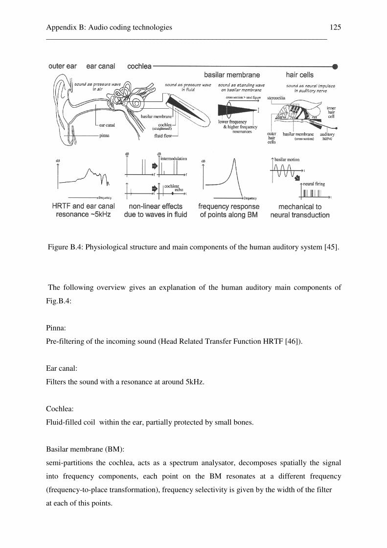
Appendix B: Audio coding technologies ________________________________________________________________________
125
Figure B.4: Physiological structure and main components of the human auditory system [45].
The following overview gives an explanation of the human auditory main components of
Fig.B.4:
Pinna:
Pre-filtering of the incoming sound (Head Related Transfer Function HRTF [46]).
Ear canal:
Filters the sound with a resonance at around 5kHz.
Cochlea:
Fluid-filled coil within the ear, partially protected by small bones.
Basilar membrane (BM):
semi-partitions the cochlea, acts as a spectrum analysator, decomposes spatially the signal
into frequency components, each point on the BM resonates at a different frequency
(frequency-to-place transformation), frequency selectivity is given by the width of the filter
at each of this points.

Appendix B: Audio coding technologies ________________________________________________________________________
126
Outer hair cells:
are distributed along the length of the BM, they change the resonant properties of the basilar
membran by reacting to feedback from the brainstorm.
Inner hair cells:
are transforming the basilar motion to neural firing, stronger motions cause more impulses,
neuronal “firing” when the basilar membran moves upwards, moment of the transformation
from physical waves to physiological information [47] transducing the sound wave at each
point into a signal on the auditory nerve.
Each cell needs a certain time to recover between firings, so the average response during a
steady tone is lower than that at its onset. Thus, the inner hair cells act as an automatically
gain control. The firing of any individual cell is pseydo-random, modulated by the movement
of the basilar membrane.
Summarizing the functions of each main components in the auditory system, the whole
human auditory sound signal processing system encodes an audio signal with relative wide
bandwidth and large dynamic range along nerves which smaller bandwidths (narrowband) and
limited dynamic ranges.The critical point is that any information lost due the transduction
process within the cochlea is not available to the brain – the cochlea is effectively a lossy
coder.
B.1.4 Psychoacoustic principles
Psychoacoustics deals with the relationship of physical sounds and how the human brain
interpret them. The field of psychoacoustics, e.g., [15], [16], [17], [47], [48], [49], [50], [51],
has made significant progress toward characterizing human auditory perception and
particularly the time-frequency analysis capabilities of the inner ear. A model of the human
perceptual behavior of music using psychoacoustic findings is presented in together with
methods to compute the similarity between two pieces of music. An auditory model for
assessing the perceived quality of coded audio signals by simulating the functionality of the
human ear and its characteristics is presented in [45], where they predict the audible and
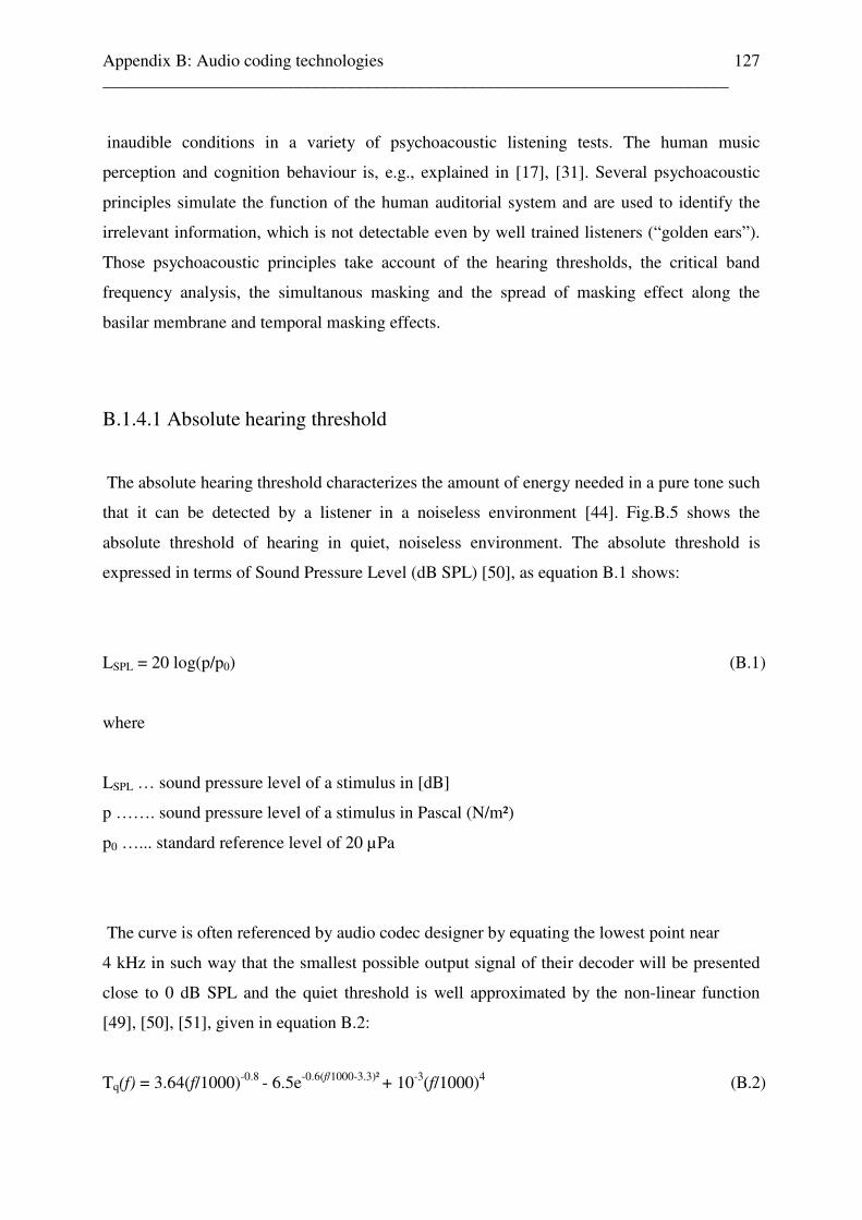
Appendix B: Audio coding technologies ________________________________________________________________________
127
inaudible conditions in a variety of psychoacoustic listening tests. The human music
perception and cognition behaviour is, e.g., explained in [17], [31]. Several psychoacoustic
principles simulate the function of the human auditorial system and are used to identify the
irrelevant information, which is not detectable even by well trained listeners (“golden ears”).
Those psychoacoustic principles take account of the hearing thresholds, the critical band
frequency analysis, the simultanous masking and the spread of masking effect along the
basilar membrane and temporal masking effects.
B.1.4.1 Absolute hearing threshold
The absolute hearing threshold characterizes the amount of energy needed in a pure tone such
that it can be detected by a listener in a noiseless environment [44]. Fig.B.5 shows the
absolute threshold of hearing in quiet, noiseless environment. The absolute threshold is
expressed in terms of Sound Pressure Level (dB SPL) [50], as equation B.1 shows:
LSPL = 20 log(p/p0) (B.1)
where
LSPL … sound pressure level of a stimulus in [dB]
p ……. sound pressure level of a stimulus in Pascal (N/m²)
p0 …... standard reference level of 20 µPa
The curve is often referenced by audio codec designer by equating the lowest point near
4 kHz in such way that the smallest possible output signal of their decoder will be presented
close to 0 dB SPL and the quiet threshold is well approximated by the non-linear function
[49], [50], [51], given in equation B.2:
Tq(f) = 3.64(f/1000)-0.8 - 6.5e-0.6(f/1000-3.3)² + 10-3(f/1000)4 (B.2)
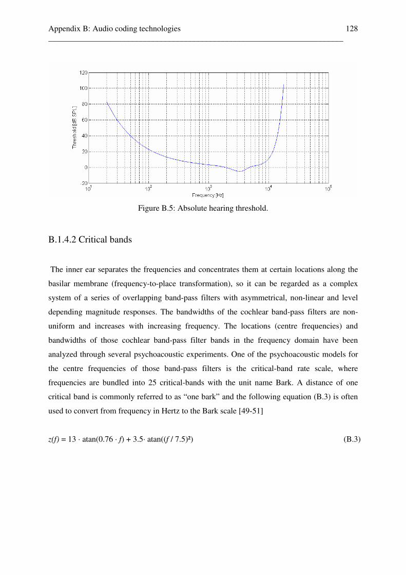
Appendix B: Audio coding technologies ________________________________________________________________________
128
Figure B.5: Absolute hearing threshold.
B.1.4.2 Critical bands
The inner ear separates the frequencies and concentrates them at certain locations along the
basilar membrane (frequency-to-place transformation), so it can be regarded as a complex
system of a series of overlapping band-pass filters with asymmetrical, non-linear and level
depending magnitude responses. The bandwidths of the cochlear band-pass filters are non-
uniform and increases with increasing frequency. The locations (centre frequencies) and
bandwidths of those cochlear band-pass filter bands in the frequency domain have been
analyzed through several psychoacoustic experiments. One of the psychoacoustic models for
the centre frequencies of those band-pass filters is the critical-band rate scale, where
frequencies are bundled into 25 critical-bands with the unit name Bark. A distance of one
critical band is commonly referred to as “one bark” and the following equation (B.3) is often
used to convert from frequency in Hertz to the Bark scale [49-51]
z(f) = 13 · atan(0.76 · f) + 3.5· atan((f / 7.5)²) (B.3)

Appendix B: Audio coding technologies ________________________________________________________________________
129
The Bark scale is a nonlinear scale that describes the nonlinear, logarithmic sound processing
in the ear and Table B.1 gives an overview of the centre frequencies and bandwidths for each
of the 25 Bark bands [49-51], while Fig.B.6 shows this Hertz to Bark scale transformation
Band
No.
Centre
Freq.
[kHz]
Bandwidth
[Hz]
Band
No.
Centre
Freq.
[kHz]
Bandwidth
[Hz]
Band
No.
Centre
Freq.
[kHz]
Bandwidth
[kHz]
1 50 0 - 100 10 1.175 1.80 - 1.27 19 4.8 4.4 - 5.3
2 150 100 - 200 11 1.37 1.27 - 1.48 20 5.8 5.3 - 6.4
3 250 200 - 300 12 1.6 1.48 - 1.72 21 7.0 6.4 - 7.7
4 350 300 - 400 13 1.85 1.72 - 2.0 22 8.5 7.7 - 9.5
5 450 400 - 510 14 2.15 2.0 - 2.32 23 10.5 9.5 - 12
6 570 510 - 630 15 2.5 2.32 - 2.7 24 13.5 12 - 15.5
7 700 630 - 770 16 2.9 2.7 - 3.15 25 19.5 15.5 -
8 840 770 - 920 17 4.3 3.15 - 3.7
9 1000 920 - 1080 18 4.0 3.7 - 4.4
Table B.1: Centre frequencies and bandwidth for each of the 25 Bark bands.
Figure B.6: Hertz to Bark Band Transformation.
Appendix B: Audio coding technologies ________________________________________________________________________
130
The “critical bandwidth” is a function of the frequency that quantifies the cochlear band-pass
filter and is conveniently approximated by equation (B.4) [49-51]
BWc(f) = 25+75[1+1.4(f/1000)²]0.69 (B.4)
B.1.4.3 Masking phenomens
Masking is the phenomenon where the perception of one sound is obscured by the perception
of another sound and can be explained in the frequency- and time domain.
B.1.4.3.1 Frequency masking
Simultaneous masking and the spread of masking refers to a frequency-domain phenomen
that can be observed whenever two or more stimuli are simultaneously presented to the
auditory system. The response of the auditory system is nonlinear and the perception of a
given tone is affected by the presence of other tones. The auditory channels for different tones
interfere with each other, giving rise to a complex auditory response called frequency
masking. That means, that a single (masking) tone is surrounded by its so-called masking
threshold curve and masking bandwidth, which intersect the threshold of the hearing curve at
two points. Every single tone within this masking bandwidth with its sound pressure level
SPL falling below the masking curve will be overshadowed (or "masked") and will not be
audible. The masking bandwidth depends on the frequency of the masking tone and increases
with the SPL-value of the masking tone. Thus, louder tones with higher frequencies will mask
more neighbouring frequencies than softer tones with lower frequencies. So, ignoring the
frequency components in the masking band whose levels fall below the masking curve does
not cause any perceptual loss. Masking phenomens are explained and shown in [44], [48],
[46], [50-51].
B.1.4.4 Temporal masking
Temporal masking explains the masking effect of a softer test tone by the presence of a
stronger one (mask tone) in the time-domain. The level of the masked signal depends on the
time between the masker and the test tone. The stronger tone will mask softer tones with
Appendix B: Audio coding technologies ________________________________________________________________________
131
lower levels, which appears a short time later (decaying time). This temporal masking effect
based on the functionality of the human auditory system, that the inner hair cells within the
human ear needs a "recovery time" from the strong mask tone, until they are able to realize
the existence of the softer test tone. In the case of audio signals, abrupt signal transients create
pre- and post- masking regions in time during which a listener will not perceive signals
beneath the audibility thresholds produced by the masker. Pre- or “backward masking” is
based on processing times in the ear and means, that signals just before the strong masker
appears are masked [46].
B.1.5 Audio Codecs based on psychoacoustic models
Audio codecs based on psychoacoustic models tries to take advantage of the way the human
auditory system perceives sound. Those lossy or loss less audio codecs take advantage of the
perceptual characteristics of the human auditory system like absolute hearing threshold,
simultaneous masking, spread of masking along the basilar membrane and temporal masking,
as descriped above. Those psychoacoustic phenomens are implemented in the audio codec
encoder side in form of a psychoacoustic model, controlling the quantization, encoding, and
reduction process of the redundant bits for the final outgoing bitstream. Comparing with
speech coding technologies the general problem in audio coding is, that no unified source
model for audio signal production exists, as for the case of speech signals.
B.1.5.1 Audio coding standards
As mentioned above, audio codec design is influenced by the resulting perceptual coding
quality, application constraints (one-way vs. two-way communications, playback, streaming,
etc.), signal characteristics, implementation complexity, and resiliency to communication
errors [44]. International standards for high-quality and high-compression perceptual audio
coding has been produced by the Moving Pictures Experts Group (MPEG), and the activities
of this standardization body have been culminated in a number of successful and popular
coding standards. In 1992, the MPEG-1 audio standard was completed and in 1994, its
backward-compatible extension MPEG-2 BC was finalized. A further, more efficient audio
coding standard is MPEG-2AAC, while the audio codec standard MPEG-4 was issued in
1999. These standards support audio encoding for a wide range of data rates and are used in
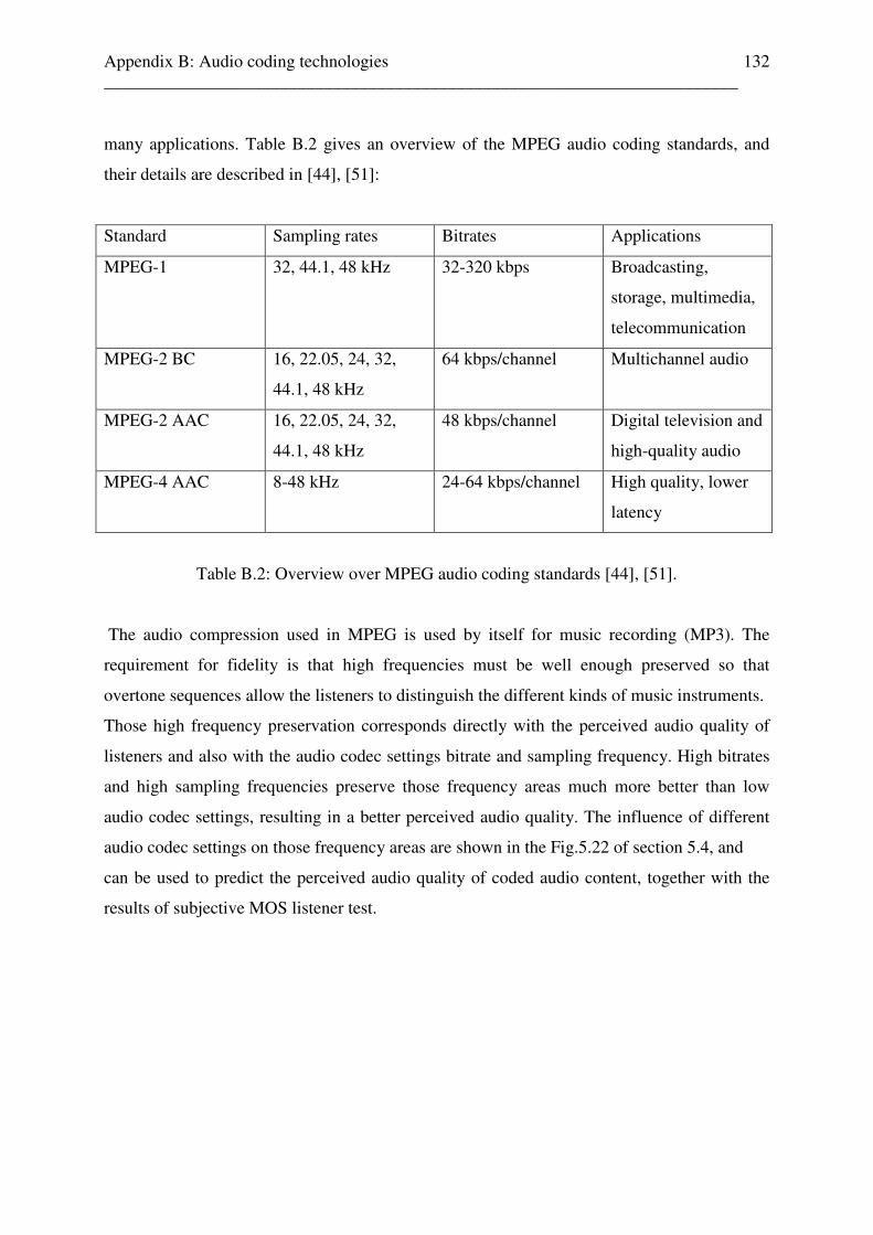
Appendix B: Audio coding technologies ________________________________________________________________________
132
many applications. Table B.2 gives an overview of the MPEG audio coding standards, and
their details are described in [44], [51]:
Standard Sampling rates Bitrates Applications
MPEG-1 32, 44.1, 48 kHz 32-320 kbps Broadcasting,
storage, multimedia,
telecommunication
MPEG-2 BC 16, 22.05, 24, 32,
44.1, 48 kHz
64 kbps/channel Multichannel audio
MPEG-2 AAC 16, 22.05, 24, 32,
44.1, 48 kHz
48 kbps/channel Digital television and
high-quality audio
MPEG-4 AAC 8-48 kHz 24-64 kbps/channel High quality, lower
latency
Table B.2: Overview over MPEG audio coding standards [44], [51].
The audio compression used in MPEG is used by itself for music recording (MP3). The
requirement for fidelity is that high frequencies must be well enough preserved so that
overtone sequences allow the listeners to distinguish the different kinds of music instruments.
Those high frequency preservation corresponds directly with the perceived audio quality of
listeners and also with the audio codec settings bitrate and sampling frequency. High bitrates
and high sampling frequencies preserve those frequency areas much more better than low
audio codec settings, resulting in a better perceived audio quality. The influence of different
audio codec settings on those frequency areas are shown in the Fig.5.22 of section 5.4, and
can be used to predict the perceived audio quality of coded audio content, together with the
results of subjective MOS listener test.

Appendix C: Matlab implementation of the reference free audio quality estimation system ________________________________________________________________________
133
Appendix C
Matlab implementation of the reference free
audio quality estimation system
C.1 Overview
The whole reference free audio quality estimation system, realized by MATLAB files or
functions, can be applied for predicting the perceived audio quality of
- each audio file from an audio file list (cf. appendix C.2), consisting of different audio
codecs, codec settings and contents (audio_quality.m)
- for a specific single audio file (audio_quality_single_audiofile.m)
- a randomly generated coded audio file, where audio codec, audio codec settings, and
audio content are randomly generated (aq_rcc.m)
- an audio sequence and each audio scene extracted from a video clip (audio_video.m).
For all those MATLAB programs, the data source, on which the coded audio .wav and
video .avi files are stored, can be chosen individually.

Appendix C: Matlab implementation of the reference free audio quality estimation system ________________________________________________________________________
134
C.2 Different coded audio content test file setup
For testing the whole audio quality estimation system, the following 349 different coded
audio files with different audio content were used (all_cod_cont.txt):
aac\8000\speech_1_teledoc.wav aac\8000\speech_2_teledoc.wav aac\8000\speech_angel.wav aac\8000\speech_astrology.wav aac\8000\speech_bayern.wav aac\8000\speech_cnn_1.wav aac\8000\speech_cnn_2.wav aac\8000\speech_cnn_3.wav aac\8000\speech_euronews_1.wav aac\8000\speech_eurosport_1.wav aac\8000\speech_eurosport_2.wav aac\8000\speech_HSE24.wav aac\8000\speech_kika_1.wav aac\8000\speech_kika_2.wav aac\8000\speech_matrix_1.wav aac\8000\speech_matrix_2.wav aac\8000\speech_roy.wav aac\8000\speech_sat1.wav aac\8000\speech_stadt.wav aac\8000\speech_zib_1.wav aac\8000\speech_zib_2.wav aac\8000\speech_zib_boerse.wav aac\16000\speech_1_teledoc.wav aac\16000\speech_2_teledoc.wav aac\16000\speech_angel.wav aac\16000\speech_astrology.wav aac\16000\speech_bayern.wav aac\16000\speech_cnn_1.wav aac\16000\speech_cnn_2.wav aac\16000\speech_cnn_3.wav aac\16000\speech_euronews_1.wav aac\16000\speech_eurosport_1.wav aac\16000\speech_eurosport_2.wav aac\16000\speech_HSE24.wav aac\16000\speech_kika_1.wav aac\16000\speech_kika_2.wav aac\16000\speech_matrix_1.wav aac\16000\speech_matrix_2.wav aac\16000\speech_roy.wav aac\16000\speech_sat1.wav aac\16000\speech_stadt.wav aac\16000\speech_zib_1.wav aac\16000\speech_zib_2.wav aac\16000\speech_zib_boerse.wav aac\20000\speech_1_teledoc.wav aac\20000\speech_2_teledoc.wav aac\20000\speech_angel.wav aac\20000\speech_astrology.wav aac\20000\speech_bayern.wav aac\20000\speech_cnn_1.wav
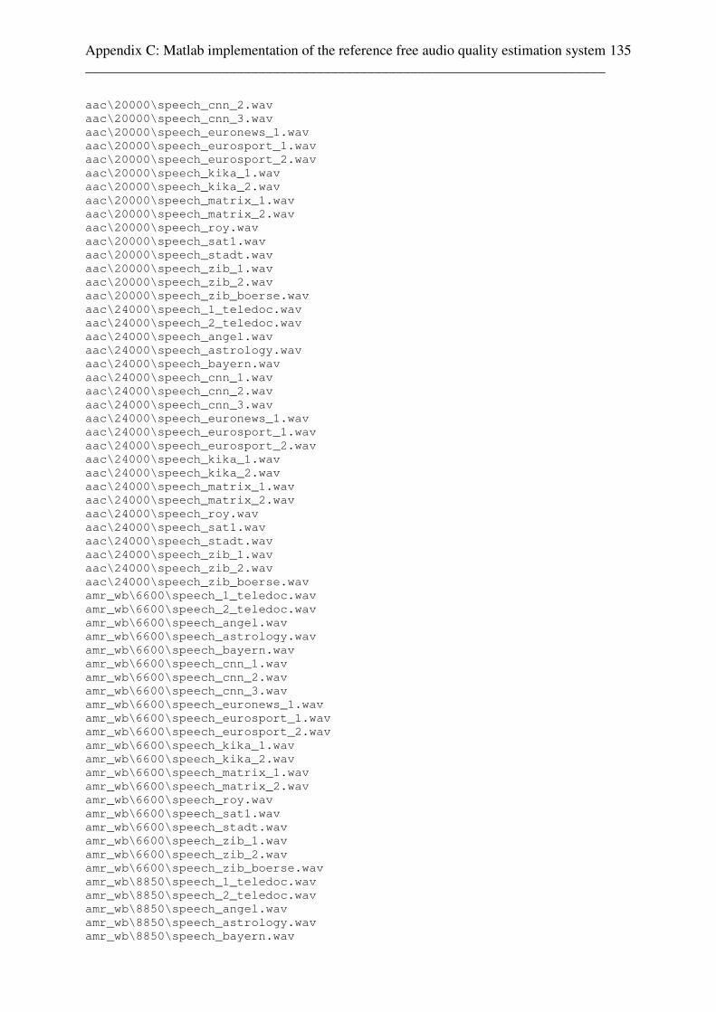
Appendix C: Matlab implementation of the reference free audio quality estimation system ________________________________________________________________________
135
aac\20000\speech_cnn_2.wav aac\20000\speech_cnn_3.wav aac\20000\speech_euronews_1.wav aac\20000\speech_eurosport_1.wav aac\20000\speech_eurosport_2.wav aac\20000\speech_kika_1.wav aac\20000\speech_kika_2.wav aac\20000\speech_matrix_1.wav aac\20000\speech_matrix_2.wav aac\20000\speech_roy.wav aac\20000\speech_sat1.wav aac\20000\speech_stadt.wav aac\20000\speech_zib_1.wav aac\20000\speech_zib_2.wav aac\20000\speech_zib_boerse.wav aac\24000\speech_1_teledoc.wav aac\24000\speech_2_teledoc.wav aac\24000\speech_angel.wav aac\24000\speech_astrology.wav aac\24000\speech_bayern.wav aac\24000\speech_cnn_1.wav aac\24000\speech_cnn_2.wav aac\24000\speech_cnn_3.wav aac\24000\speech_euronews_1.wav aac\24000\speech_eurosport_1.wav aac\24000\speech_eurosport_2.wav aac\24000\speech_kika_1.wav aac\24000\speech_kika_2.wav aac\24000\speech_matrix_1.wav aac\24000\speech_matrix_2.wav aac\24000\speech_roy.wav aac\24000\speech_sat1.wav aac\24000\speech_stadt.wav aac\24000\speech_zib_1.wav aac\24000\speech_zib_2.wav aac\24000\speech_zib_boerse.wav amr_wb\6600\speech_1_teledoc.wav amr_wb\6600\speech_2_teledoc.wav amr_wb\6600\speech_angel.wav amr_wb\6600\speech_astrology.wav amr_wb\6600\speech_bayern.wav amr_wb\6600\speech_cnn_1.wav amr_wb\6600\speech_cnn_2.wav amr_wb\6600\speech_cnn_3.wav amr_wb\6600\speech_euronews_1.wav amr_wb\6600\speech_eurosport_1.wav amr_wb\6600\speech_eurosport_2.wav amr_wb\6600\speech_kika_1.wav amr_wb\6600\speech_kika_2.wav amr_wb\6600\speech_matrix_1.wav amr_wb\6600\speech_matrix_2.wav amr_wb\6600\speech_roy.wav amr_wb\6600\speech_sat1.wav amr_wb\6600\speech_stadt.wav amr_wb\6600\speech_zib_1.wav amr_wb\6600\speech_zib_2.wav amr_wb\6600\speech_zib_boerse.wav amr_wb\8850\speech_1_teledoc.wav amr_wb\8850\speech_2_teledoc.wav amr_wb\8850\speech_angel.wav amr_wb\8850\speech_astrology.wav amr_wb\8850\speech_bayern.wav
Appendix C: Matlab implementation of the reference free audio quality estimation system ________________________________________________________________________
136
amr_wb\8850\speech_cnn_1.wav amr_wb\8850\speech_cnn_2.wav amr_wb\8850\speech_cnn_3.wav amr_wb\8850\speech_euronews_1.wav amr_wb\8850\speech_eurosport_1.wav amr_wb\8850\speech_eurosport_2.wav amr_wb\8850\speech_kika_1.wav amr_wb\8850\speech_kika_2.wav amr_wb\8850\speech_matrix_1.wav amr_wb\8850\speech_matrix_2.wav amr_wb\8850\speech_roy.wav amr_wb\8850\speech_sat1.wav amr_wb\8850\speech_stadt.wav amr_wb\8850\speech_zib_1.wav amr_wb\8850\speech_zib_2.wav amr_wb\8850\speech_zib_boerse.wav amr_wb\12650\speech_1_teledoc.wav amr_wb\12650\speech_2_teledoc.wav amr_wb\12650\speech_angel.wav amr_wb\12650\speech_astrology.wav amr_wb\12650\speech_bayern.wav amr_wb\12650\speech_cnn_1.wav amr_wb\12650\speech_cnn_2.wav amr_wb\12650\speech_cnn_3.wav amr_wb\12650\speech_euronews_1.wav amr_wb\12650\speech_eurosport_1.wav amr_wb\12650\speech_eurosport_2.wav amr_wb\12650\speech_kika_1.wav amr_wb\12650\speech_kika_2.wav amr_wb\12650\speech_matrix_1.wav amr_wb\12650\speech_matrix_2.wav amr_wb\12650\speech_roy.wav amr_wb\12650\speech_sat1.wav amr_wb\12650\speech_stadt.wav amr_wb\12650\speech_zib_1.wav amr_wb\12650\speech_zib_2.wav amr_wb\12650\speech_zib_boerse.wav amr_wb\15850\speech_1_teledoc.wav amr_wb\15850\speech_2_teledoc.wav amr_wb\15850\speech_angel.wav amr_wb\15850\speech_astrology.wav amr_wb\15850\speech_bayern.wav amr_wb\15850\speech_cnn_1.wav amr_wb\15850\speech_cnn_2.wav amr_wb\15850\speech_cnn_3.wav amr_wb\15850\speech_euronews_1.wav amr_wb\15850\speech_eurosport_1.wav amr_wb\15850\speech_eurosport_2.wav amr_wb\15850\speech_kika_1.wav amr_wb\15850\speech_kika_2.wav amr_wb\15850\speech_matrix_1.wav amr_wb\15850\speech_matrix_2.wav amr_wb\15850\speech_roy.wav amr_wb\15850\speech_sat1.wav amr_wb\15850\speech_stadt.wav amr_wb\15850\speech_zib_1.wav amr_wb\15850\speech_zib_2.wav amr_wb\15850\speech_zib_boerse.wav amr_nb\4750\speech_1_teledoc.wav amr_nb\4750\speech_2_teledoc.wav amr_nb\4750\speech_angel.wav amr_nb\4750\speech_astrology.wav
Appendix C: Matlab implementation of the reference free audio quality estimation system ________________________________________________________________________
137
amr_nb\4750\speech_bayern.wav amr_nb\4750\speech_cnn_1.wav amr_nb\4750\speech_cnn_2.wav amr_nb\4750\speech_cnn_3.wav amr_nb\4750\speech_euronews_1.wav amr_nb\4750\speech_eurosport_1.wav amr_nb\4750\speech_eurosport_2.wav amr_nb\4750\speech_kika_1.wav amr_nb\4750\speech_kika_2.wav amr_nb\4750\speech_matrix_1.wav amr_nb\4750\speech_matrix_2.wav amr_nb\4750\speech_roy.wav amr_nb\4750\speech_sat1.wav amr_nb\4750\speech_stadt.wav amr_nb\4750\speech_zib_1.wav amr_nb\4750\speech_zib_2.wav amr_nb\4750\speech_zib_boerse.wav amr_nb\7950\speech_1_teledoc.wav amr_nb\7950\speech_2_teledoc.wav amr_nb\7950\speech_angel.wav amr_nb\7950\speech_astrology.wav amr_nb\7950\speech_bayern.wav amr_nb\7950\speech_cnn_1.wav amr_nb\7950\speech_cnn_2.wav amr_nb\7950\speech_cnn_3.wav amr_nb\7950\speech_euronews_1.wav amr_nb\7950\speech_eurosport_1.wav amr_nb\7950\speech_eurosport_2.wav amr_nb\7950\speech_kika_1.wav amr_nb\7950\speech_kika_2.wav amr_nb\7950\speech_matrix_1.wav amr_nb\7950\speech_matrix_2.wav amr_nb\7950\speech_roy.wav amr_nb\7950\speech_sat1.wav amr_nb\7950\speech_stadt.wav amr_nb\7950\speech_zib_1.wav amr_nb\7950\speech_zib_2.wav amr_nb\7950\speech_zib_boerse.wav amr_nb\12200\speech_1_teledoc.wav amr_nb\12200\speech_2_teledoc.wav amr_nb\12200\speech_angel.wav amr_nb\12200\speech_astrology.wav amr_nb\12200\speech_bayern.wav amr_nb\12200\speech_cnn_1.wav amr_nb\12200\speech_cnn_2.wav amr_nb\12200\speech_cnn_3.wav amr_nb\12200\speech_euronews_1.wav amr_nb\12200\speech_eurosport_1.wav amr_nb\12200\speech_eurosport_2.wav amr_nb\12200\speech_kika_1.wav amr_nb\12200\speech_kika_2.wav amr_nb\12200\speech_matrix_1.wav amr_nb\12200\speech_matrix_2.wav amr_nb\12200\speech_roy.wav amr_nb\12200\speech_sat1.wav amr_nb\12200\speech_stadt.wav amr_nb\12200\speech_zib_1.wav amr_nb\12200\speech_zib_2.wav amr_nb\12200\speech_zib_boerse.wav aac\8000\classic_music_haydn aac\8000\classic_music_orf_1 aac\8000\classic_music_panorama
Appendix C: Matlab implementation of the reference free audio quality estimation system ________________________________________________________________________
138
aac\8000\classic_music_teledoc aac\8000\classic_music_tw1 aac\8000\classic_music_zib_1 aac\8000\classic_music_zib_2 aac\16000\classic_music_haydn aac\16000\classic_music_orf_1 aac\16000\classic_music_panorama aac\16000\classic_music_teledoc aac\16000\classic_music_tw1 aac\16000\classic_music_zib_1 aac\16000\classic_music_zib_2 aac\20000\classic_music_haydn aac\20000\classic_music_orf_1 aac\20000\classic_music_panorama aac\20000\classic_music_teledoc aac\20000\classic_music_tw1 aac\20000\classic_music_zib_1 aac\20000\classic_music_zib_2 aac\24000\classic_music_haydn aac\24000\classic_music_orf_1 aac\24000\classic_music_panorama aac\24000\classic_music_teledoc aac\24000\classic_music_tw1 aac\24000\classic_music_zib_1 aac\24000\classic_music_zib_2 amr_wb\6600\classic_music_haydn amr_wb\6600\classic_music_orf_1 amr_wb\6600\classic_music_panorama amr_wb\6600\classic_music_teledoc amr_wb\6600\classic_music_zib_1 amr_wb\6600\classic_music_zib_2 amr_wb\8850\classic_music_haydn amr_wb\8850\classic_music_orf_1 amr_wb\8850\classic_music_panorama amr_wb\8850\classic_music_teledoc amr_wb\8850\classic_music_zib_1 amr_wb\8850\classic_music_zib_2 amr_wb\12650\classic_music_haydn amr_wb\12650\classic_music_orf_1 amr_wb\12650\classic_music_panorama amr_wb\12650\classic_music_teledoc amr_wb\12650\classic_music_zib_1 amr_wb\12650\classic_music_zib_2 amr_wb\15850\classic_music_haydn amr_wb\15850\classic_music_orf_1 amr_wb\15850\classic_music_panorama amr_wb\15850\classic_music_teledoc amr_wb\15850\classic_music_zib_1 amr_wb\15850\classic_music_zib_2 aac\8000\other_music_FA aac\8000\other_music_f4 aac\8000\other_music_matrix_1 aac\8000\other_music_matrix_2 aac\8000\other_music_roy aac\16000\other_music_FA aac\16000\other_music_f4 aac\16000\other_music_matrix_1 aac\16000\other_music_matrix_2 aac\16000\other_music_roy aac\20000\other_music_FA aac\20000\other_music_f4 aac\20000\other_music_matrix_1
Appendix C: Matlab implementation of the reference free audio quality estimation system ________________________________________________________________________
139
aac\20000\other_music_matrix_2 aac\20000\other_music_roy aac\24000\other_music_FA aac\24000\other_music_f4 aac\24000\other_music_matrix_1 aac\24000\other_music_matrix_2 aac\24000\other_music_roy amr_wb\6600\other_music_FA amr_wb\6600\other_music_f4 amr_wb\6600\other_music_matrix_2 amr_wb\6600\other_music_roy mr_wb\8850\other_music_FA amr_wb\8850\other_music_f4 amr_wb\8850\other_music_matrix_2 amr_wb\8850\other_music_roy amr_wb\12650\other_music_FA amr_wb\12650\other_music_f4 amr_wb\12650\other_music_matrix_2 amr_wb\12650\other_music_roy amr_wb\15850\other_music_FA amr_wb\15850\other_music_f4 amr_wb\15850\other_music_matrix_2 amr_wb\15850\other_music_roy aac\8000\non_speech_stadion_euronews_1.wav aac\8000\non_speech_stadion_eurosport_1.wav aac\8000\non_speech_fx_kika_1.wav aac\8000\non_speech_fx_matrix.wav aac\16000\non_speech_stadion_euronews_1.wav aac\16000\non_speech_stadion_eurosport_1.wav aac\16000\non_speech_fx_kika_1.wav aac\16000\non_speech_fx_matrix.wav aac\20000\non_speech_stadion_euronews_1.wav aac\20000\non_speech_stadion_eurosport_1.wav aac\20000\non_speech_fx_kika_1.wav aac\20000\non_speech_fx_matrix.wav aac\24000\non_speech_stadion_euronews_1.wav aac\24000\non_speech_stadion_eurosport_1.wav aac\24000\non_speech_fx_kika_1.wav aac\24000\non_speech_fx_matrix.wav amr_wb\6600\non_speech_stadion_euronews_1.wav amr_wb\6600\non_speech_stadion_eurosport_1.wav amr_wb\6600\non_speech_fx_kika_1.wav amr_wb\8850\non_speech_stadion_euronews_1.wav amr_wb\8850\non_speech_stadion_eurosport_1.wav amr_wb\8850\non_speech_fx_kika_1.wav amr_wb\12650\non_speech_stadion_euronews_1.wav amr_wb\12650\non_speech_stadion_eurosport_1.wav amr_wb\12650\non_speech_fx_kika_1.wav amr_wb\15850\non_speech_stadion_euronews_1.wav amr_wb\15850\non_speech_stadion_eurosport_1.wav amr_wb\15850\non_speech_fx_kika_1.wav
Single files from this list were also chosen to test audio_quality_single_audiofile.m
Appendix C: Matlab implementation of the reference free audio quality estimation system ________________________________________________________________________
140
C.3 audio_quality.m
This MATLAB main program realizes the reference free prediction of the audio codec, audio
codec settings, bitrate, sampling frequency, audio content, and audio quality of each audio file
from a file list, for unknown (‘rb_est’) or known audio codec settings (‘rb_extr’). The
coded .wav files and the audio lists are stored in different folders at the same location
(‘C:\audio\’, ‘C:\audio_quality_audio_list’), and the audio list must be imported to the
workspace. The following syntax gives an example of the audio .wav file path and name,
C:\audio\amr_nb\4750\speech_stadt.wav
and the MATLAB file audio_quality.m is called from the command line by
audio_quality(selected_cod_cont_F,
'selected_cod_cont_F_txt','selected_cod_cont_F_xls','rb_est');
if the .wav files and audio file list are stored at location F:\ and the audio codec settings are
unknown. Program results are written to the .txt and .xls files 'selected_cod_cont_F_txt', and
'selected_cod_cont_F_xls', and program outputs for each audio file from the list are similar to
those, which are presented in appendix C.4.
C.4 audio_quality_single_audio_file.m
This MATLAB program predicts the audio codec, audio codec settings, audio content, and
audio quality of one single audio file with known or unknown audio codec settings. Path and
name of the audio .wav file are similar to those described in appendix C.3, and the MATLAB
file is called from the command line by
audio_quality_single_audiofile('F:\audio\amr_nb\4750\speech_stadt.wav',
'speech_4750_txt', 'speech_4750_xls', 'rb_est');

Appendix C: Matlab implementation of the reference free audio quality estimation system ________________________________________________________________________
141
for the case of unknown audio codec settings. Detail results of the reference free audio quality
estimation for one specific coded audio file are given in the following program output:
--------------------------------------------------------------------------------------------------------------------------
-- AUDIO CODEC, CONTENT, BITRATE, SAMPLING FREQUENCY AND AUDIO QUALITY -
-- ESTIMATION / CLASSIFICATION PROCESS OF .wav FILE --
-- C: \aac\8000\speech_stadt.wav --
--------------------------------------------------------------------------------------------------------------------------
ZERO CROSSING RATE STATISTICS FOR CONTENT CLASSIFICATION (SPEECH / NON SPEECH)
zcr_std_modified_audiofile : 0.17746
zcr_mean_modified_audiofile : 0.25215
ratio_zcr_std_mean_modified_audiofile : 0.70379
zcr_std_orig_audiofile : 0.064761
zcr_mean_orig_audiofile : 0.1129
ratio_zcr_std_mean_orig_audiofile : 0.57362
FREQUENCY DOMAIN STATISTIC FOR CONTENT CLASSIFICATION (CLASSIC/OTHER MUSIC, FX
SOUNDS)
mcf_orig : 355.1897
mbw_orig : 318.9002
ratio_mcf_mbw_orig : 1.1138
PHASE STATISTICS I FOR AMR WB / AMR NB AND SAMPLING FREQUENCY CLASSIFICATION
std_phase_rad_orig : 0.20716
mean_phase_rad_orig : 0.0068241
ratio_phase_std_mean_orig : 30.3567
PHASE STATISTIC II
mcp_orig : 2975.0453
mpw_orig : 781.4233
ratio_mcp_mpw_orig : 3.8072
C:aac\8000\speech_stadt.wav
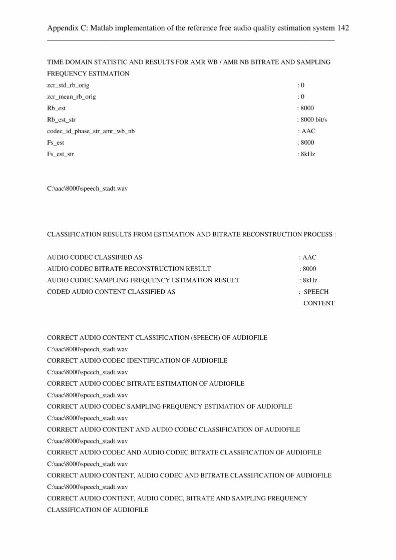
Appendix C: Matlab implementation of the reference free audio quality estimation system ________________________________________________________________________
142
TIME DOMAIN STATISTIC AND RESULTS FOR AMR WB / AMR NB BITRATE AND SAMPLING
FREQUENCY ESTIMATION
zcr_std_rb_orig : 0
zcr_mean_rb_orig : 0
Rb_est : 8000
Rb_est_str : 8000 bit/s
codec_id_phase_str_amr_wb_nb : AAC
Fs_est : 8000
Fs_est_str : 8kHz
C:\aac\8000\speech_stadt.wav
CLASSIFICATION RESULTS FROM ESTIMATION AND BITRATE RECONSTRUCTION PROCESS :
AUDIO CODEC CLASSIFIED AS : AAC
AUDIO CODEC BITRATE RECONSTRUCTION RESULT : 8000
AUDIO CODEC SAMPLING FREQUENCY ESTIMATION RESULT : 8kHz
CODED AUDIO CONTENT CLASSIFIED AS : SPEECH
CONTENT
CORRECT AUDIO CONTENT CLASSIFICATION (SPEECH) OF AUDIOFILE
C:\aac\8000\speech_stadt.wav
CORRECT AUDIO CODEC IDENTIFICATION OF AUDIOFILE
C:\aac\8000\speech_stadt.wav
CORRECT AUDIO CODEC BITRATE ESTIMATION OF AUDIOFILE
C:\aac\8000\speech_stadt.wav
CORRECT AUDIO CODEC SAMPLING FREQUENCY ESTIMATION OF AUDIOFILE
C:\aac\8000\speech_stadt.wav
CORRECT AUDIO CONTENT AND AUDIO CODEC CLASSIFICATION OF AUDIOFILE
C:\aac\8000\speech_stadt.wav
CORRECT AUDIO CODEC AND AUDIO CODEC BITRATE CLASSIFICATION OF AUDIOFILE
C:\aac\8000\speech_stadt.wav
CORRECT AUDIO CONTENT, AUDIO CODEC AND BITRATE CLASSIFICATION OF AUDIOFILE
C:\aac\8000\speech_stadt.wav
CORRECT AUDIO CONTENT, AUDIO CODEC, BITRATE AND SAMPLING FREQUENCY
CLASSIFICATION OF AUDIOFILE
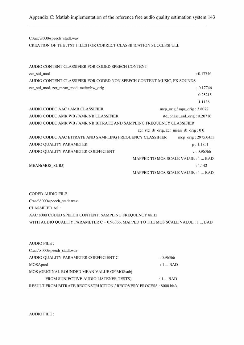
Appendix C: Matlab implementation of the reference free audio quality estimation system ________________________________________________________________________
143
C:\aac\8000\speech_stadt.wav
CREATION OF THE .TXT FILES FOR CORRECT CLASSIFICATION SUCCESSFULL
AUDIO CONTENT CLASSIFIER FOR CODED SPEECH CONTENT
zcr_std_mod : 0.17746
AUDIO CONTENT CLASSIFIER FOR CODED NON SPEECH CONTENT MUSIC, FX SOUNDS
zcr_std_mod, zcr_mean_mod, mcf/mbw_orig : 0.17746
0.25215
1.1138
AUDIO CODEC AAC / AMR CLASSIFIER mcp_orig / mpr_orig : 3.8072
AUDIO CODEC AMR WB / AMR NB CLASSIFIER std_phase_rad_orig : 0.20716
AUDIO CODEC AMR WB / AMR NB BITRATE AND SAMPLING FREQUENCY CLASSIFIER
zcr_std_rb_orig, zcr_mean_rb_orig : 0 0
AUDIO CODEC AAC BITRATE AND SAMPLING FREQUENCY CLASSIFIER mcp_orig : 2975.0453
AUDIO QUALITY PARAMETER p : 1.1851
AUDIO QUALITY PARAMETER COEFFICIENT c : 0.96366
MAPPED TO MOS SCALE VALUE : 1 ... BAD
MEAN(MOS_SUBJ) : 1.142
MAPPED TO MOS SCALE VALUE : 1 ... BAD
CODED AUDIO FILE
C:aac\8000\speech_stadt.wav
CLASSIFIED AS :
AAC 8000 CODED SPEECH CONTENT, SAMPLING FREQUENCY 8kHz
WITH AUDIO QUALITY PARAMETER C = 0.96366, MAPPED TO THE MOS SCALE VALUE : 1 ... BAD
AUDIO FILE :
C:aac\8000\speech_stadt.wav
AUDIO QUALITY PARAMETER COEFFICIENT C : 0.96366
MOSApred : 1 ... BAD
MOS (ORIGINAL ROUNDED MEAN VALUE OF MOSsubj
FROM SUBJECTIVE AUDIO LISTENER TESTS) : 1 ... BAD
RESULT FROM BITRATE RECONSTRUCTION / RECOVERY PROCESS : 8000 bit/s
AUDIO FILE :
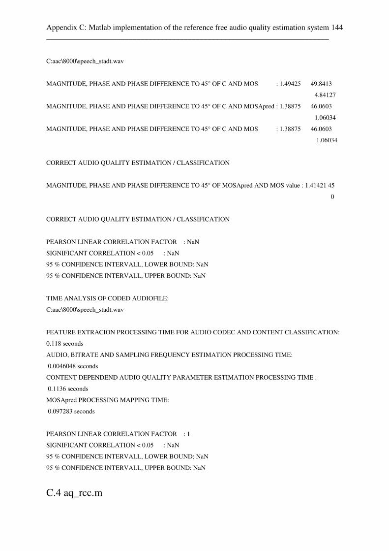
Appendix C: Matlab implementation of the reference free audio quality estimation system ________________________________________________________________________
144
C:aac\8000\speech_stadt.wav
MAGNITUDE, PHASE AND PHASE DIFFERENCE TO 45° OF C AND MOS : 1.49425 49.8413
4.84127
MAGNITUDE, PHASE AND PHASE DIFFERENCE TO 45° OF C AND MOSApred : 1.38875 46.0603
1.06034
MAGNITUDE, PHASE AND PHASE DIFFERENCE TO 45° OF C AND MOS : 1.38875 46.0603
1.06034
CORRECT AUDIO QUALITY ESTIMATION / CLASSIFICATION
MAGNITUDE, PHASE AND PHASE DIFFERENCE TO 45° OF MOSApred AND MOS value : 1.41421 45
0
CORRECT AUDIO QUALITY ESTIMATION / CLASSIFICATION
PEARSON LINEAR CORRELATION FACTOR : NaN
SIGNIFICANT CORRELATION < 0.05 : NaN
95 % CONFIDENCE INTERVALL, LOWER BOUND: NaN
95 % CONFIDENCE INTERVALL, UPPER BOUND: NaN
TIME ANALYSIS OF CODED AUDIOFILE:
C:aac\8000\speech_stadt.wav
FEATURE EXTRACION PROCESSING TIME FOR AUDIO CODEC AND CONTENT CLASSIFICATION:
0.118 seconds
AUDIO, BITRATE AND SAMPLING FREQUENCY ESTIMATION PROCESSING TIME:
0.0046048 seconds
CONTENT DEPENDEND AUDIO QUALITY PARAMETER ESTIMATION PROCESSING TIME :
0.1136 seconds
MOSApred PROCESSING MAPPING TIME:
0.097283 seconds
PEARSON LINEAR CORRELATION FACTOR : 1
SIGNIFICANT CORRELATION < 0.05 : NaN
95 % CONFIDENCE INTERVALL, LOWER BOUND: NaN
95 % CONFIDENCE INTERVALL, UPPER BOUND: NaN
C.4 aq_rcc.m
Appendix C: Matlab implementation of the reference free audio quality estimation system ________________________________________________________________________
145
This MATLAB program creates a randomly coded audio file with randomly chosen audio
codec, audio codec settings and audio content and predicts the perceived audio quality of such
an audio file, and the MATLAB file is called from the command line by
aq_rcc('F');
where the location, on which the audio .wav files are stored, is given by the input parameter.
C.5 audio_video.m
This MATLAB program extends the whole reference free audio quality estimation system for
the prediction of the audio codecs, audio codec settings, audio contents, and audio qualities of
each scene in an audio sequence extracted from a video clip, for known or unknown audio
codec settings. Further, the overall audio codec, audio codec settings, audio content, and
audio quality are predictably. All .avi video files are stored at location ‘datasource:\video\’,
and all .wav audio files are stored at location ‘datasource:\audio\’. The MATLAB file is
called fom the command line by
audio_video('angel_clip.avi','amr_nb\7950\angel_clip.wav', 1024, 'rb_est','F');
using a 1024 FFT.
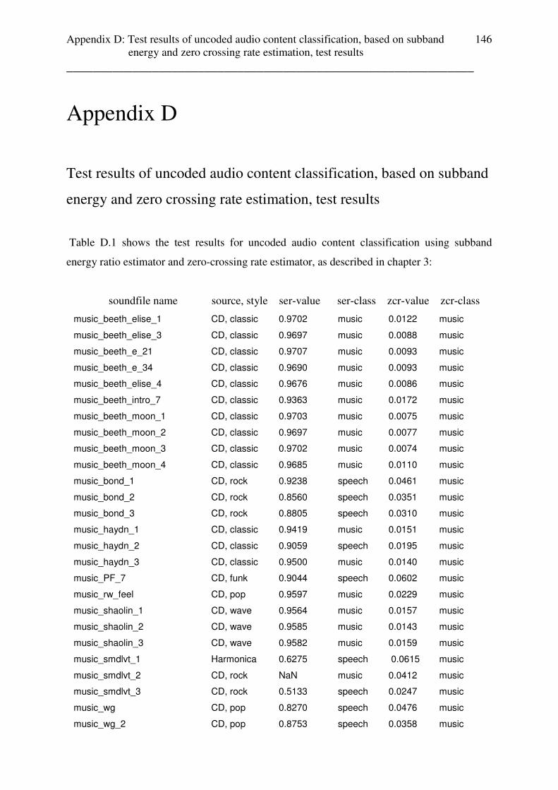
Appendix D: Test results of uncoded audio content classification, based on subband energy and zero crossing rate estimation, test results ______________________________________________________________
146
Appendix D
Test results of uncoded audio content classification, based on subband
energy and zero crossing rate estimation, test results
Table D.1 shows the test results for uncoded audio content classification using subband
energy ratio estimator and zero-crossing rate estimator, as described in chapter 3:
soundfile name source, style ser-value ser-class zcr-value zcr-class
music_beeth_elise_1 CD, classic 0.9702 music 0.0122 music
music_beeth_elise_3 CD, classic 0.9697 music 0.0088 music
music_beeth_e_21 CD, classic 0.9707 music 0.0093 music
music_beeth_e_34 CD, classic 0.9690 music 0.0093 music
music_beeth_elise_4 CD, classic 0.9676 music 0.0086 music
music_beeth_intro_7 CD, classic 0.9363 music 0.0172 music
music_beeth_moon_1 CD, classic 0.9703 music 0.0075 music
music_beeth_moon_2 CD, classic 0.9697 music 0.0077 music
music_beeth_moon_3 CD, classic 0.9702 music 0.0074 music
music_beeth_moon_4 CD, classic 0.9685 music 0.0110 music
music_bond_1 CD, rock 0.9238 speech 0.0461 music
music_bond_2 CD, rock 0.8560 speech 0.0351 music
music_bond_3 CD, rock 0.8805 speech 0.0310 music
music_haydn_1 CD, classic 0.9419 music 0.0151 music
music_haydn_2 CD, classic 0.9059 speech 0.0195 music
music_haydn_3 CD, classic 0.9500 music 0.0140 music
music_PF_7 CD, funk 0.9044 speech 0.0602 music
music_rw_feel CD, pop 0.9597 music 0.0229 music
music_shaolin_1 CD, wave 0.9564 music 0.0157 music
music_shaolin_2 CD, wave 0.9585 music 0.0143 music
music_shaolin_3 CD, wave 0.9582 music 0.0159 music
music_smdlvt_1 Harmonica 0.6275 speech 0.0615 music
music_smdlvt_2 CD, rock NaN music 0.0412 music
music_smdlvt_3 CD, rock 0.5133 speech 0.0247 music
music_wg CD, pop 0.8270 speech 0.0476 music
music_wg_2 CD, pop 0.8753 speech 0.0358 music

Appendix D: Test results of uncoded audio content classification, based on subband energy and zero crossing rate estimation, test results ______________________________________________________________
147
music_wg_10ms CD, pop 0.9278 speech 0.0214 music
music_wg_10ms2 CD, pop 0.6667 speech 0.0432 music
music_ziria_summer CD, techno 0.8199 speech 0.0541 music
music_ziria_5ms CD, techno 0.8817 speech 0.0064 music
music_ziria_100ms CD, techno 0.7348 speech 0.0619 music
music_cm_piano CD, classic 0.9687 music 0.0109 music
music_frozen_1 CD, wave 0.9446 music 0.0159 music
music_frozen_2 CD, wave 0.9437 music 0.0160 music
music_psb_sin CD, pop 0.7634 speech 0.0414 music
music_psb_rent CD, pop 0.9209 speech 0.0329 music
music_phenomena CD, electro NaN music 0.0114 music
music_voc_lml_7 CD, dance 0.8445 speech 0.0551 music
music_Tspiel_1 V, ethno NaN music 0.0109 music
music_Tspiel_2 V, ethno NaN music 0.0132 music
music_Tspiel_3 V, ethno 0.8851 speech 0.0248 music
music_Tspiel_4 V, ethno 0.8382 speech 0.0232 music
music_Tspiel_5 V, ethno NaN music 0.0309 music
music_Tspiel_6 V, ethno 0.7396 speech 0.0300 music
music_Tspiel_7 V, ethno 0.6602 speech 0.0352 music
music_Tspiel_8 V, ethno 0.9064 speech 0.0242 music
music_Tspiel_9 V, ethno 0.8498 speech 0.0261 music
music_Tspiel_10 V, ethno 0.9272 speech 0.0211 music
music_Tmillion_1 V, electro 0.8369 speech 0.0331 music
music_Tmillion_2 V, electro 0.9454 speech 0.0256 music
music_Tmillion_3 V, electro NaN music 0.0161 music
music_Tmillion_4 V, rock 0.9699 music 0.0057 music
music_Tmillion_5 V, fx NaN music 0.0172 music
music_Tmillion_6 V, fx 0.9322 music 0.0070 music
music_Tmillion_7 V, beat NaN music 0.0158 music
music_Tmillion_8 V, beat 0.9570 music 0.0188 music
music_Tmillion_9 V, fx 0.8971 speech 0.0136 music
music_Tmillion_10 V, fx 0.9291 speech 0.0261 music
music_Tmillion_11 V, fx 0.8535 speech 0.0350 music
music_Tmillion_12 V, rock NaN music 0.0134 music
music_Tmillion_13 V, bono U2 0.9459 music 0.0192 music
music_Tmillion_1 V, bono U2 0.9129 speech 0.0185 music
music_Tmillion_15 V, bono U2 0.9051 speech 0.0179 music
music_Tmillion_16 V, bono U2 0.9155 speech 0.0190 music
music_Tjurney_1 V, ethno 0.9356 music 0.0145 music
music_Tjurney_2 V, ethno 0.9390 music 0.0142 music

Appendix D: Test results of uncoded audio content classification, based on subband energy and zero crossing rate estimation, test results ______________________________________________________________
148
music_Tjurney_3 V, ethno 0.4667 speech 0.0684 music
music_Tjurney_4 V, ethno 0.9026 speech 0.0438 music
music_Tjurney_5 V, ethno 0.9427 music 0.0189 music
music_Tjurney_6 V, ethno 0.9135 speech 0.0194 music
music_Tgreen_1 V, orchestra NaN music 0.0189 music
music_Tgreen_2 V, orchestra 0.8957 speech 0.0200 music
music_Tgreen_3 V, orchestra 0.8646 speech 0.0217 music
music_Tgreen_4 V, orchestra 0.7809 speech 0.0277 music
music_Tgreen_5 V, orchestra 0.8777 speech 0.0246 music
music_Tgreen_6 V, orchestra 0.7819 speech 0.0276 music
music_Tgreen_7 V, orchestra 0.8198 speech 0.0350 music
music_Tend_1 V, orchestra 0.9672 music 0.0091 music
music_Tend_2 V, orchestra 0.8787 speech 0.0231 music
music_Tend_3 V, orchestra NaN speech 0.0188 music
music_Tend_4 V, orchestra 0.8536 speech 0.0189 music
music_Tend_5 V, orchestra 0.8808 speech 0.0271 music
music_Tend_6 V, orchestra 0.8794 speech 0.0286 music
music_Tend_7 V, orchestra NaN music 0.0252 music
music_Tbeach_1 V, orchestra 0.9372 music 0.0178 music
music_Tbeach_2 V, orchestra 0.9498 music 0.0182 music
music_Tbeach_3 V, orchestra 0.9370 music 0.0257 music
music_Tbeach_4 V, orchestra 0.9533 music 0.0191 music
music_Tbeach_5 V, orchestra 0.9515 music 0.0218 music
music_Tbeach_6 V, rock 0.9562 music 0.0222 music
music_Tbeach_7 V, rock 0.9435 music 0.0230 music
music_Tbeach_8 V, rock 0.9434 music 0.0227 music
music_Tbeach_9 V, spheric 0.6976 speech 0.0264 music
music_Tbeach_10 V, fx 0.9690 music 0.0087 music
music_Tbeach_11 V, fx 0.9500 music 0.0176 music
music_Tbeach_12 V, fx 0.8337 speech 0.0333 music
music_Tbeach_13 V, spheric 0.8009 speech 0.0329 music
music_Tbeach_14 V, spheric 0.9631 music 0.0163 music
music_smoothy_1 V, rock 0.8297 speech 0.0592 music
music_smoothy_2 V, hit 0.6740 speech 0.0813 music
music_smoothy_3 V, beat 0.8158 speech 0.0837 music
music_smoothy_4 V, voc 0.4116 speech 0.0896 music
music_sleepy_10s V, spheric NaN music 0.0179 music
music_sleepy_5s V, orchestra 0.9333 music 0.0223 music
music_sleepy_4 V, fx 0.6252 speech 0.0628 music
music_sleepy_3 V, orchestra 0.9034 speech 0.0231 music
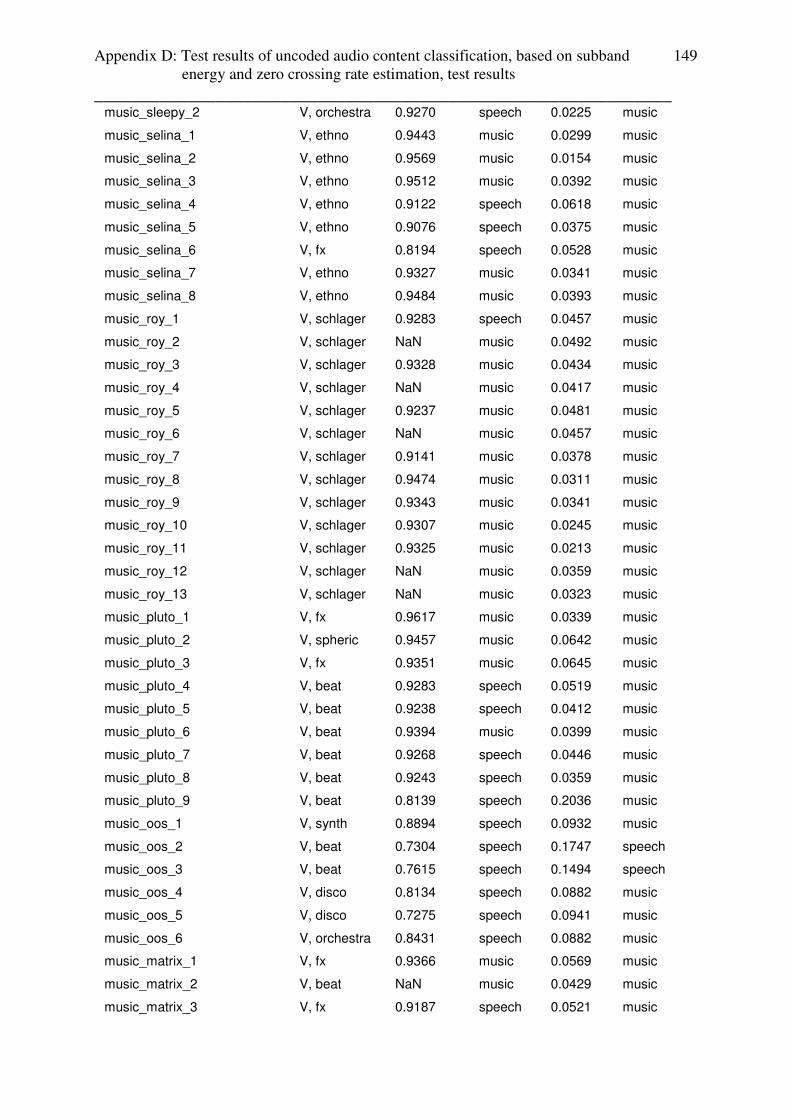
Appendix D: Test results of uncoded audio content classification, based on subband energy and zero crossing rate estimation, test results ______________________________________________________________
149
music_sleepy_2 V, orchestra 0.9270 speech 0.0225 music
music_selina_1 V, ethno 0.9443 music 0.0299 music
music_selina_2 V, ethno 0.9569 music 0.0154 music
music_selina_3 V, ethno 0.9512 music 0.0392 music
music_selina_4 V, ethno 0.9122 speech 0.0618 music
music_selina_5 V, ethno 0.9076 speech 0.0375 music
music_selina_6 V, fx 0.8194 speech 0.0528 music
music_selina_7 V, ethno 0.9327 music 0.0341 music
music_selina_8 V, ethno 0.9484 music 0.0393 music
music_roy_1 V, schlager 0.9283 speech 0.0457 music
music_roy_2 V, schlager NaN music 0.0492 music
music_roy_3 V, schlager 0.9328 music 0.0434 music
music_roy_4 V, schlager NaN music 0.0417 music
music_roy_5 V, schlager 0.9237 music 0.0481 music
music_roy_6 V, schlager NaN music 0.0457 music
music_roy_7 V, schlager 0.9141 music 0.0378 music
music_roy_8 V, schlager 0.9474 music 0.0311 music
music_roy_9 V, schlager 0.9343 music 0.0341 music
music_roy_10 V, schlager 0.9307 music 0.0245 music
music_roy_11 V, schlager 0.9325 music 0.0213 music
music_roy_12 V, schlager NaN music 0.0359 music
music_roy_13 V, schlager NaN music 0.0323 music
music_pluto_1 V, fx 0.9617 music 0.0339 music
music_pluto_2 V, spheric 0.9457 music 0.0642 music
music_pluto_3 V, fx 0.9351 music 0.0645 music
music_pluto_4 V, beat 0.9283 speech 0.0519 music
music_pluto_5 V, beat 0.9238 speech 0.0412 music
music_pluto_6 V, beat 0.9394 music 0.0399 music
music_pluto_7 V, beat 0.9268 speech 0.0446 music
music_pluto_8 V, beat 0.9243 speech 0.0359 music
music_pluto_9 V, beat 0.8139 speech 0.2036 music
music_oos_1 V, synth 0.8894 speech 0.0932 music
music_oos_2 V, beat 0.7304 speech 0.1747 speech
music_oos_3 V, beat 0.7615 speech 0.1494 speech
music_oos_4 V, disco 0.8134 speech 0.0882 music
music_oos_5 V, disco 0.7275 speech 0.0941 music
music_oos_6 V, orchestra 0.8431 speech 0.0882 music
music_matrix_1 V, fx 0.9366 music 0.0569 music
music_matrix_2 V, beat NaN music 0.0429 music
music_matrix_3 V, fx 0.9187 speech 0.0521 music
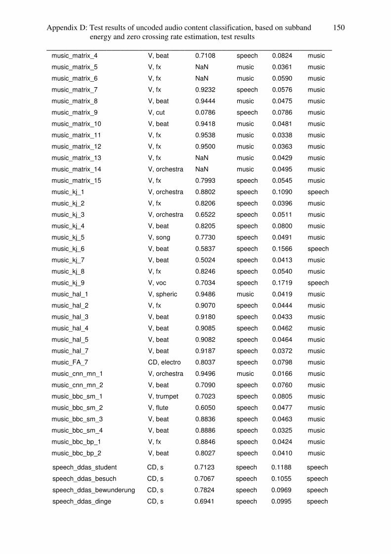
Appendix D: Test results of uncoded audio content classification, based on subband energy and zero crossing rate estimation, test results ______________________________________________________________
150
music_matrix_4 V, beat 0.7108 speech 0.0824 music
music_matrix_5 V, fx NaN music 0.0361 music
music_matrix_6 V, fx NaN music 0.0590 music
music_matrix_7 V, fx 0.9232 speech 0.0576 music
music_matrix_8 V, beat 0.9444 music 0.0475 music
music_matrix_9 V, cut 0.0786 speech 0.0786 music
music_matrix_10 V, beat 0.9418 music 0.0481 music
music_matrix_11 V, fx 0.9538 music 0.0338 music
music_matrix_12 V, fx 0.9500 music 0.0363 music
music_matrix_13 V, fx NaN music 0.0429 music
music_matrix_14 V, orchestra NaN music 0.0495 music
music_matrix_15 V, fx 0.7993 speech 0.0545 music
music_kj_1 V, orchestra 0.8802 speech 0.1090 speech
music_kj_2 V, fx 0.8206 speech 0.0396 music
music_kj_3 V, orchestra 0.6522 speech 0.0511 music
music_kj_4 V, beat 0.8205 speech 0.0800 music
music_kj_5 V, song 0.7730 speech 0.0491 music
music_kj_6 V, beat 0.5837 speech 0.1566 speech
music_kj_7 V, beat 0.5024 speech 0.0413 music
music_kj_8 V, fx 0.8246 speech 0.0540 music
music_kj_9 V, voc 0.7034 speech 0.1719 speech
music_hal_1 V, spheric 0.9486 music 0.0419 music
music_hal_2 V, fx 0.9070 speech 0.0444 music
music_hal_3 V, beat 0.9180 speech 0.0433 music
music_hal_4 V, beat 0.9085 speech 0.0462 music
music_hal_5 V, beat 0.9082 speech 0.0464 music
music_hal_7 V, beat 0.9187 speech 0.0372 music
music_FA_7 CD, electro 0.8037 speech 0.0798 music
music_cnn_mn_1 V, orchestra 0.9496 music 0.0166 music
music_cnn_mn_2 V, beat 0.7090 speech 0.0760 music
music_bbc_sm_1 V, trumpet 0.7023 speech 0.0805 music
music_bbc_sm_2 V, flute 0.6050 speech 0.0477 music
music_bbc_sm_3 V, beat 0.8836 speech 0.0463 music
music_bbc_sm_4 V, beat 0.8886 speech 0.0325 music
music_bbc_bp_1 V, fx 0.8846 speech 0.0424 music
music_bbc_bp_2 V, beat 0.8027 speech 0.0410 music
speech_ddas_student CD, s 0.7123 speech 0.1188 speech
speech_ddas_besuch CD, s 0.7067 speech 0.1055 speech
speech_ddas_bewunderung CD, s 0.7824 speech 0.0969 speech
speech_ddas_dinge CD, s 0.6941 speech 0.0995 speech
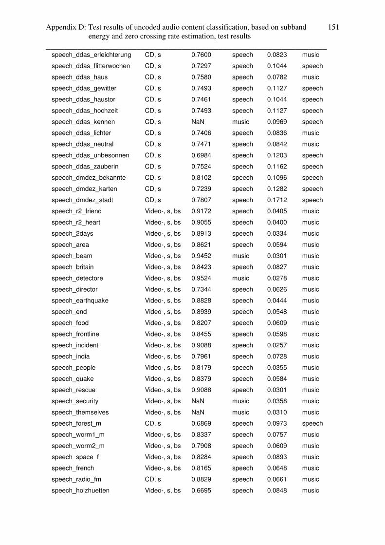
Appendix D: Test results of uncoded audio content classification, based on subband energy and zero crossing rate estimation, test results ______________________________________________________________
151
speech_ddas_erleichterung CD, s 0.7600 speech 0.0823 music
speech_ddas_flitterwochen CD, s 0.7297 speech 0.1044 speech
speech_ddas_haus CD, s 0.7580 speech 0.0782 music
speech_ddas_gewitter CD, s 0.7493 speech 0.1127 speech
speech_ddas_haustor CD, s 0.7461 speech 0.1044 speech
speech_ddas_hochzeit CD, s 0.7493 speech 0.1127 speech
speech_ddas_kennen CD, s NaN music 0.0969 speech
speech_ddas_lichter CD, s 0.7406 speech 0.0836 music
speech_ddas_neutral CD, s 0.7471 speech 0.0842 music
speech_ddas_unbesonnen CD, s 0.6984 speech 0.1203 speech
speech_ddas_zauberin CD, s 0.7524 speech 0.1162 speech
speech_dmdez_bekannte CD, s 0.8102 speech 0.1096 speech
speech_dmdez_karten CD, s 0.7239 speech 0.1282 speech
speech_dmdez_stadt CD, s 0.7807 speech 0.1712 speech
speech_r2_friend Video-, s, bs 0.9172 speech 0.0405 music
speech_r2_heart Video-, s, bs 0.9055 speech 0.0400 music
speech_2days Video-, s, bs 0.8913 speech 0.0334 music
speech_area Video-, s, bs 0.8621 speech 0.0594 music
speech_beam Video-, s, bs 0.9452 music 0.0301 music
speech_britain Video-, s, bs 0.8423 speech 0.0827 music
speech_detectore Video-, s, bs 0.9524 music 0.0278 music
speech_director Video-, s, bs 0.7344 speech 0.0626 music
speech_earthquake Video-, s, bs 0.8828 speech 0.0444 music
speech_end Video-, s, bs 0.8939 speech 0.0548 music
speech_food Video-, s, bs 0.8207 speech 0.0609 music
speech_frontline Video-, s, bs 0.8455 speech 0.0598 music
speech_incident Video-, s, bs 0.9088 speech 0.0257 music
speech_india Video-, s, bs 0.7961 speech 0.0728 music
speech_people Video-, s, bs 0.8179 speech 0.0355 music
speech_quake Video-, s, bs 0.8379 speech 0.0584 music
speech_rescue Video-, s, bs 0.9088 speech 0.0301 music
speech_security Video-, s, bs NaN music 0.0358 music
speech_themselves Video-, s, bs NaN music 0.0310 music
speech_forest_m CD, s 0.6869 speech 0.0973 speech
speech_worm1_m Video-, s, bs 0.8337 speech 0.0757 music
speech_worm2_m Video-, s, bs 0.7908 speech 0.0609 music
speech_space_f Video-, s, bs 0.8284 speech 0.0893 music
speech_french Video-, s, bs 0.8165 speech 0.0648 music
speech_radio_fm CD, s 0.8829 speech 0.0661 music
speech_holzhuetten Video-, s, bs 0.6695 speech 0.0848 music
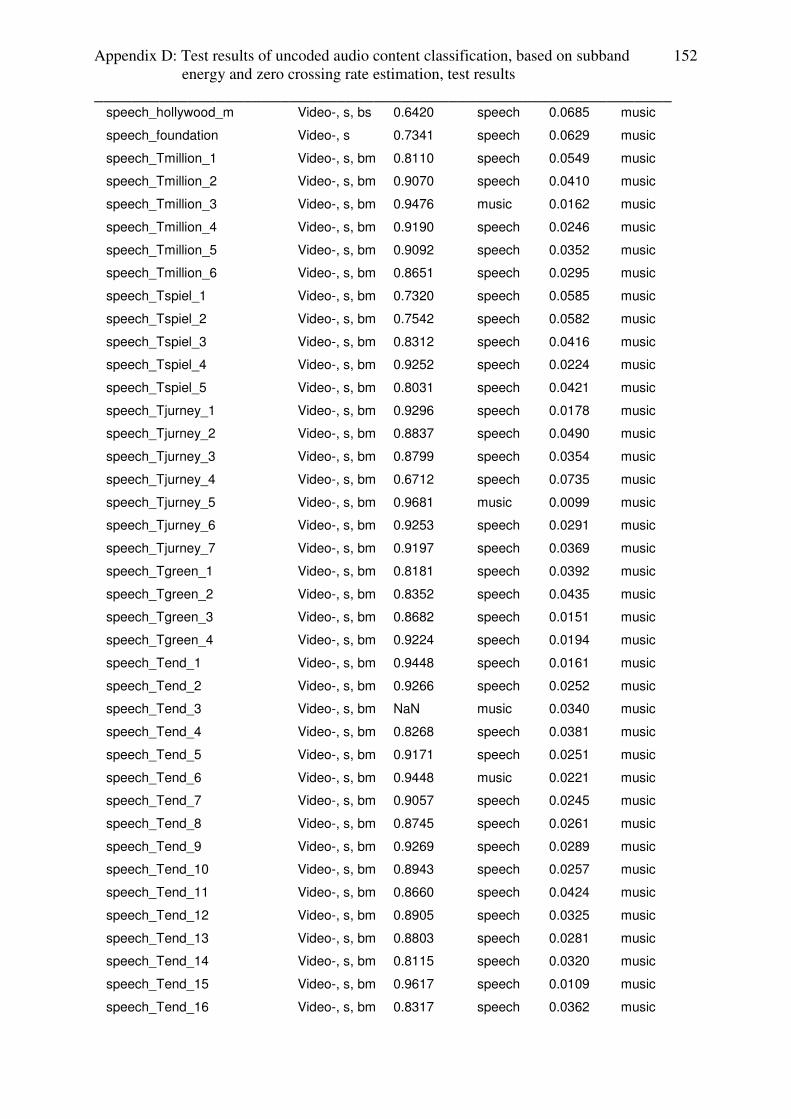
Appendix D: Test results of uncoded audio content classification, based on subband energy and zero crossing rate estimation, test results ______________________________________________________________
152
speech_hollywood_m Video-, s, bs 0.6420 speech 0.0685 music
speech_foundation Video-, s 0.7341 speech 0.0629 music
speech_Tmillion_1 Video-, s, bm 0.8110 speech 0.0549 music
speech_Tmillion_2 Video-, s, bm 0.9070 speech 0.0410 music
speech_Tmillion_3 Video-, s, bm 0.9476 music 0.0162 music
speech_Tmillion_4 Video-, s, bm 0.9190 speech 0.0246 music
speech_Tmillion_5 Video-, s, bm 0.9092 speech 0.0352 music
speech_Tmillion_6 Video-, s, bm 0.8651 speech 0.0295 music
speech_Tspiel_1 Video-, s, bm 0.7320 speech 0.0585 music
speech_Tspiel_2 Video-, s, bm 0.7542 speech 0.0582 music
speech_Tspiel_3 Video-, s, bm 0.8312 speech 0.0416 music
speech_Tspiel_4 Video-, s, bm 0.9252 speech 0.0224 music
speech_Tspiel_5 Video-, s, bm 0.8031 speech 0.0421 music
speech_Tjurney_1 Video-, s, bm 0.9296 speech 0.0178 music
speech_Tjurney_2 Video-, s, bm 0.8837 speech 0.0490 music
speech_Tjurney_3 Video-, s, bm 0.8799 speech 0.0354 music
speech_Tjurney_4 Video-, s, bm 0.6712 speech 0.0735 music
speech_Tjurney_5 Video-, s, bm 0.9681 music 0.0099 music
speech_Tjurney_6 Video-, s, bm 0.9253 speech 0.0291 music
speech_Tjurney_7 Video-, s, bm 0.9197 speech 0.0369 music
speech_Tgreen_1 Video-, s, bm 0.8181 speech 0.0392 music
speech_Tgreen_2 Video-, s, bm 0.8352 speech 0.0435 music
speech_Tgreen_3 Video-, s, bm 0.8682 speech 0.0151 music
speech_Tgreen_4 Video-, s, bm 0.9224 speech 0.0194 music
speech_Tend_1 Video-, s, bm 0.9448 speech 0.0161 music
speech_Tend_2 Video-, s, bm 0.9266 speech 0.0252 music
speech_Tend_3 Video-, s, bm NaN music 0.0340 music
speech_Tend_4 Video-, s, bm 0.8268 speech 0.0381 music
speech_Tend_5 Video-, s, bm 0.9171 speech 0.0251 music
speech_Tend_6 Video-, s, bm 0.9448 music 0.0221 music
speech_Tend_7 Video-, s, bm 0.9057 speech 0.0245 music
speech_Tend_8 Video-, s, bm 0.8745 speech 0.0261 music
speech_Tend_9 Video-, s, bm 0.9269 speech 0.0289 music
speech_Tend_10 Video-, s, bm 0.8943 speech 0.0257 music
speech_Tend_11 Video-, s, bm 0.8660 speech 0.0424 music
speech_Tend_12 Video-, s, bm 0.8905 speech 0.0325 music
speech_Tend_13 Video-, s, bm 0.8803 speech 0.0281 music
speech_Tend_14 Video-, s, bm 0.8115 speech 0.0320 music
speech_Tend_15 Video-, s, bm 0.9617 speech 0.0109 music
speech_Tend_16 Video-, s, bm 0.8317 speech 0.0362 music
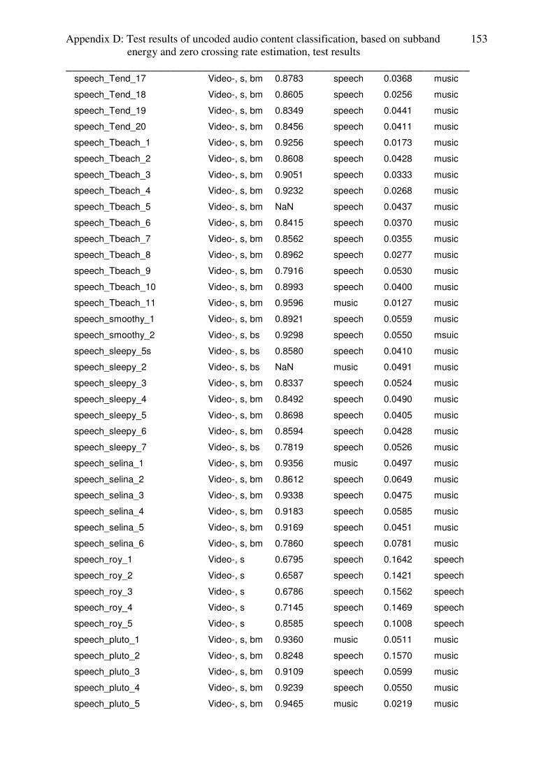
Appendix D: Test results of uncoded audio content classification, based on subband energy and zero crossing rate estimation, test results ______________________________________________________________
153
speech_Tend_17 Video-, s, bm 0.8783 speech 0.0368 music
speech_Tend_18 Video-, s, bm 0.8605 speech 0.0256 music
speech_Tend_19 Video-, s, bm 0.8349 speech 0.0441 music
speech_Tend_20 Video-, s, bm 0.8456 speech 0.0411 music
speech_Tbeach_1 Video-, s, bm 0.9256 speech 0.0173 music
speech_Tbeach_2 Video-, s, bm 0.8608 speech 0.0428 music
speech_Tbeach_3 Video-, s, bm 0.9051 speech 0.0333 music
speech_Tbeach_4 Video-, s, bm 0.9232 speech 0.0268 music
speech_Tbeach_5 Video-, s, bm NaN speech 0.0437 music
speech_Tbeach_6 Video-, s, bm 0.8415 speech 0.0370 music
speech_Tbeach_7 Video-, s, bm 0.8562 speech 0.0355 music
speech_Tbeach_8 Video-, s, bm 0.8962 speech 0.0277 music
speech_Tbeach_9 Video-, s, bm 0.7916 speech 0.0530 music
speech_Tbeach_10 Video-, s, bm 0.8993 speech 0.0400 music
speech_Tbeach_11 Video-, s, bm 0.9596 music 0.0127 music
speech_smoothy_1 Video-, s, bm 0.8921 speech 0.0559 music
speech_smoothy_2 Video-, s, bs 0.9298 speech 0.0550 msuic
speech_sleepy_5s Video-, s, bs 0.8580 speech 0.0410 music
speech_sleepy_2 Video-, s, bs NaN music 0.0491 music
speech_sleepy_3 Video-, s, bm 0.8337 speech 0.0524 music
speech_sleepy_4 Video-, s, bm 0.8492 speech 0.0490 music
speech_sleepy_5 Video-, s, bm 0.8698 speech 0.0405 music
speech_sleepy_6 Video-, s, bm 0.8594 speech 0.0428 music
speech_sleepy_7 Video-, s, bs 0.7819 speech 0.0526 music
speech_selina_1 Video-, s, bm 0.9356 music 0.0497 music
speech_selina_2 Video-, s, bm 0.8612 speech 0.0649 music
speech_selina_3 Video-, s, bm 0.9338 speech 0.0475 music
speech_selina_4 Video-, s, bm 0.9183 speech 0.0585 music
speech_selina_5 Video-, s, bm 0.9169 speech 0.0451 music
speech_selina_6 Video-, s, bm 0.7860 speech 0.0781 music
speech_roy_1 Video-, s 0.6795 speech 0.1642 speech
speech_roy_2 Video-, s 0.6587 speech 0.1421 speech
speech_roy_3 Video-, s 0.6786 speech 0.1562 speech
speech_roy_4 Video-, s 0.7145 speech 0.1469 speech
speech_roy_5 Video-, s 0.8585 speech 0.1008 speech
speech_pluto_1 Video-, s, bm 0.9360 music 0.0511 music
speech_pluto_2 Video-, s, bm 0.8248 speech 0.1570 music
speech_pluto_3 Video-, s, bm 0.9109 speech 0.0599 music
speech_pluto_4 Video-, s, bm 0.9239 speech 0.0550 music
speech_pluto_5 Video-, s, bm 0.9465 music 0.0219 music
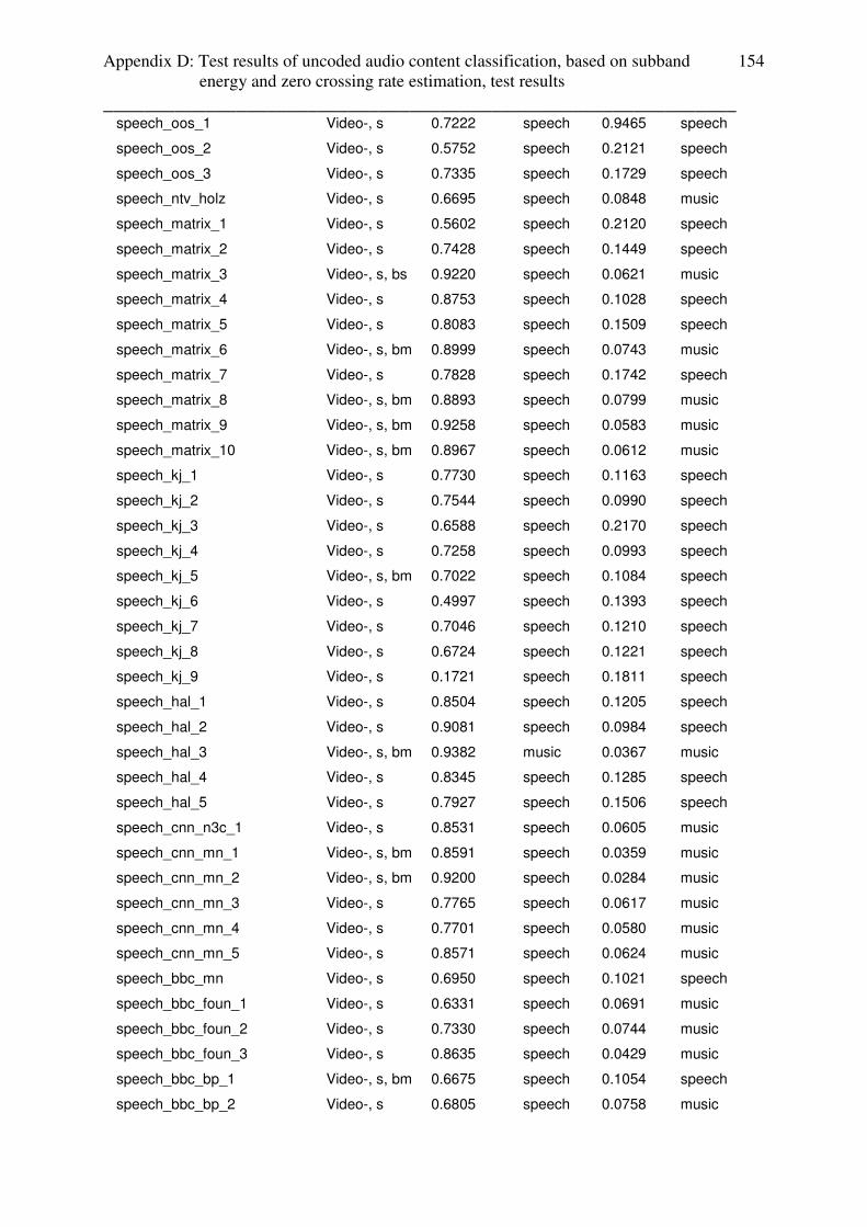
Appendix D: Test results of uncoded audio content classification, based on subband energy and zero crossing rate estimation, test results ______________________________________________________________
154
speech_oos_1 Video-, s 0.7222 speech 0.9465 speech
speech_oos_2 Video-, s 0.5752 speech 0.2121 speech
speech_oos_3 Video-, s 0.7335 speech 0.1729 speech
speech_ntv_holz Video-, s 0.6695 speech 0.0848 music
speech_matrix_1 Video-, s 0.5602 speech 0.2120 speech
speech_matrix_2 Video-, s 0.7428 speech 0.1449 speech
speech_matrix_3 Video-, s, bs 0.9220 speech 0.0621 music
speech_matrix_4 Video-, s 0.8753 speech 0.1028 speech
speech_matrix_5 Video-, s 0.8083 speech 0.1509 speech
speech_matrix_6 Video-, s, bm 0.8999 speech 0.0743 music
speech_matrix_7 Video-, s 0.7828 speech 0.1742 speech
speech_matrix_8 Video-, s, bm 0.8893 speech 0.0799 music
speech_matrix_9 Video-, s, bm 0.9258 speech 0.0583 music
speech_matrix_10 Video-, s, bm 0.8967 speech 0.0612 music
speech_kj_1 Video-, s 0.7730 speech 0.1163 speech
speech_kj_2 Video-, s 0.7544 speech 0.0990 speech
speech_kj_3 Video-, s 0.6588 speech 0.2170 speech
speech_kj_4 Video-, s 0.7258 speech 0.0993 speech
speech_kj_5 Video-, s, bm 0.7022 speech 0.1084 speech
speech_kj_6 Video-, s 0.4997 speech 0.1393 speech
speech_kj_7 Video-, s 0.7046 speech 0.1210 speech
speech_kj_8 Video-, s 0.6724 speech 0.1221 speech
speech_kj_9 Video-, s 0.1721 speech 0.1811 speech
speech_hal_1 Video-, s 0.8504 speech 0.1205 speech
speech_hal_2 Video-, s 0.9081 speech 0.0984 speech
speech_hal_3 Video-, s, bm 0.9382 music 0.0367 music
speech_hal_4 Video-, s 0.8345 speech 0.1285 speech
speech_hal_5 Video-, s 0.7927 speech 0.1506 speech
speech_cnn_n3c_1 Video-, s 0.8531 speech 0.0605 music
speech_cnn_mn_1 Video-, s, bm 0.8591 speech 0.0359 music
speech_cnn_mn_2 Video-, s, bm 0.9200 speech 0.0284 music
speech_cnn_mn_3 Video-, s 0.7765 speech 0.0617 music
speech_cnn_mn_4 Video-, s 0.7701 speech 0.0580 music
speech_cnn_mn_5 Video-, s 0.8571 speech 0.0624 music
speech_bbc_mn Video-, s 0.6950 speech 0.1021 speech
speech_bbc_foun_1 Video-, s 0.6331 speech 0.0691 music
speech_bbc_foun_2 Video-, s 0.7330 speech 0.0744 music
speech_bbc_foun_3 Video-, s 0.8635 speech 0.0429 music
speech_bbc_bp_1 Video-, s, bm 0.6675 speech 0.1054 speech
speech_bbc_bp_2 Video-, s 0.6805 speech 0.0758 music
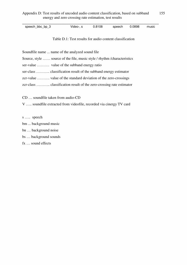
Appendix D: Test results of uncoded audio content classification, based on subband energy and zero crossing rate estimation, test results ______________________________________________________________
155
speech_bbc_bp_3 Video-, s 0.8108 speech 0.0898 music
Table D.1: Test results for audio content classification
Soundfile name ... name of the analyzed sound file
Source, style …… source of the file, music style / rhythm /characteristics
ser-value ………. value of the subband energy ratio
ser-class ……….. classification result of the subband energy estimator
zcr-value ………. value of the standard deviation of the zero-crossings
zcr-class ……….. classification result of the zero-crossing rate estimator
CD … soundfile taken from audio-CD
V ….. soundfile extracted from videofile, recorded via cinergy TV card
s ….. speech
bm ... background music
bn … background noise
bs … background sounds
fx … sound effects
Appendix E: Test results of uncoded audio content classification for audio sequences (music videos, music documentary, cinema trailers) ______________________________________________________________
156
Appendix E
Test results of uncoded audio content classification
for audio sequences
(music videos, music documentary, cinema trailers)
Table E.1 presents the test results of uncoded audio content classification for the case of
audio scenes of an audio sequence, defined by audio scene detecting cut time points using the
video tool described in chapter 6:
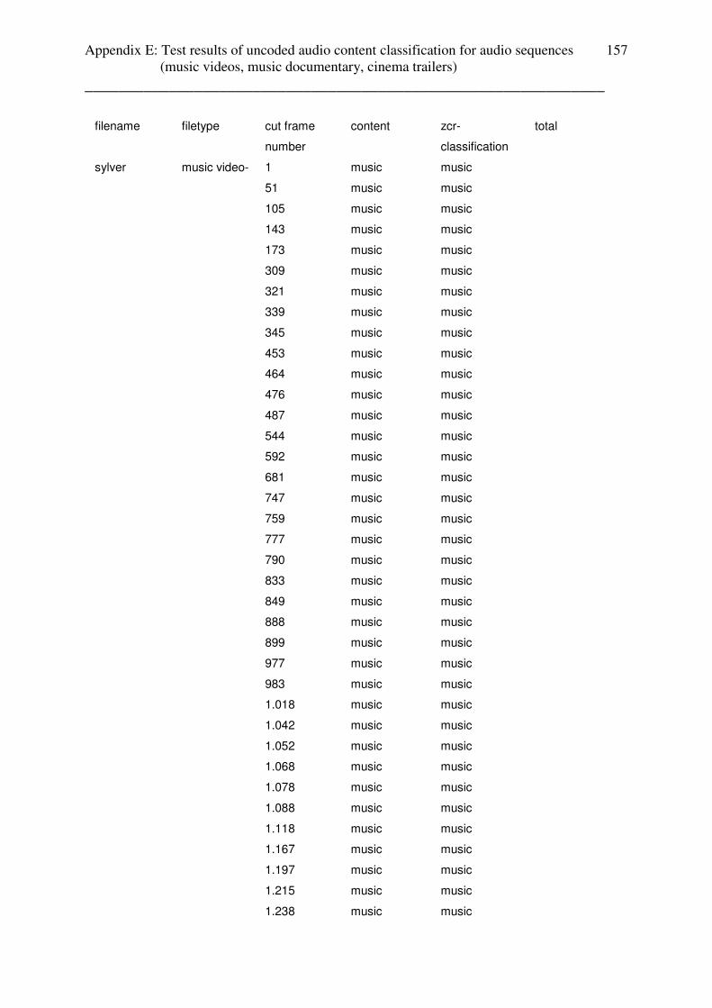
Appendix E: Test results of uncoded audio content classification for audio sequences (music videos, music documentary, cinema trailers) ______________________________________________________________
157
filename filetype cut frame
number
content zcr-
classification
total
sylver music video- 1 music music
51 music music
105 music music
143 music music
173 music music
309 music music
321 music music
339 music music
345 music music
453 music music
464 music music
476 music music
487 music music
544 music music
592 music music
681 music music
747 music music
759 music music
777 music music
790 music music
833 music music
849 music music
888 music music
899 music music
977 music music
983 music music
1.018 music music
1.042 music music
1.052 music music
1.068 music music
1.078 music music
1.088 music music
1.118 music music
1.167 music music
1.197 music music
1.215 music music
1.238 music music
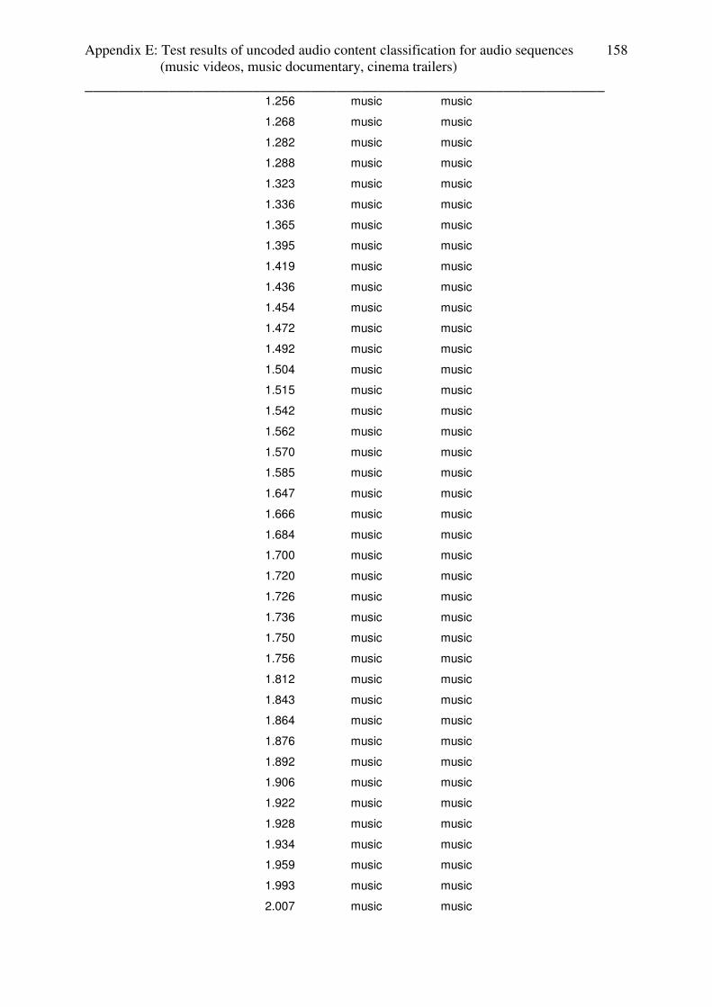
Appendix E: Test results of uncoded audio content classification for audio sequences (music videos, music documentary, cinema trailers) ______________________________________________________________
158
1.256 music music
1.268 music music
1.282 music music
1.288 music music
1.323 music music
1.336 music music
1.365 music music
1.395 music music
1.419 music music
1.436 music music
1.454 music music
1.472 music music
1.492 music music
1.504 music music
1.515 music music
1.542 music music
1.562 music music
1.570 music music
1.585 music music
1.647 music music
1.666 music music
1.684 music music
1.700 music music
1.720 music music
1.726 music music
1.736 music music
1.750 music music
1.756 music music
1.812 music music
1.843 music music
1.864 music music
1.876 music music
1.892 music music
1.906 music music
1.922 music music
1.928 music music
1.934 music music
1.959 music music
1.993 music music
2.007 music music
Appendix E: Test results of uncoded audio content classification for audio sequences (music videos, music documentary, cinema trailers) ______________________________________________________________
159
2.030 music music
2.074 music music
2.098 music music
2.127 music music
2.162 music music
2.187 music music
2.233 music music
2.245 music music
2.257 music music
2.269 music music
2.293 music music
2.313 music music
2.335 music music
2.347 music music
2.373 music music
2.413 music music
2.467 music music
2.491 music music
2.511 music music
2.533 music music
2.556 music music
2.570 music music
2.598 music music
2.678 music music
2.706 music music
2.725 music music
2.737 music music
2.755 music music
2.809 music music
2.839 music music
2.863 music music
2.893 music music
2.907 music music
2.925 music music
2.953 music music
2.971 music music
2.983 music music
3.014 music music
3.026 music music
3.082 music music
Appendix E: Test results of uncoded audio content classification for audio sequences (music videos, music documentary, cinema trailers) ______________________________________________________________
160
3.097 music music
3.203 music music
3.246 music music
3.258 music music
3.270 music music
3.311 music music
3.463 music music
3.480 music music
3.500 music music
3.517 music music
3.597 music music
3.644 music music
3.677 music music
3.849 music music
3.872 music music
3.888 music music
3.900 music music
3.914 music music
3.926 music music
3.939 music music
4.015 music music
4.021 music music
4.081 music music
4.140 music music
4.199 music music
4.253 music music
4.265 music music
4.363 music music
4.445 music music
4.493 music music
4.525 music music
4.540 music music
4.563 music music
4.601 music music
4.625 music music
4.639 music music
4.667 music music
4.679 music music
4.691 music music
4.745 music music

Appendix E: Test results of uncoded audio content classification for audio sequences (music videos, music documentary, cinema trailers) ______________________________________________________________
161
4.751 music music
4.805 music music
4.842 music music
4.967 music music
5.031 music music
5.065 music music
5.099 music music
5.141 music music
5.197 music music
5.262 music music
5.280 music music
5.316 music music
5.401 music music
5.514 music music
5.593 music music
5.621 music music 100%
pet shop boys music video- 1 music / fade in speech
154 music music
201 music music
248 music music
274 music music
345 music music
366 music music
486 music music
524 music music
574 music music
616 music music
643 music music
663 music music
689 music music
715 music music
737 music music
759 music music
812 music music
854 music music
893 music music
922 music music
952 music music
985 music music
1021 music music
Appendix E: Test results of uncoded audio content classification for audio sequences (music videos, music documentary, cinema trailers) ______________________________________________________________
162
1059 music music
1109 music music
1159 music music
1190 music music
1251 music music
1299 music music
1364 music music
1405 music music
1441 music music
1476 music music
1491 music music
1525 music music
1557 music music
1625 music music
1682 music music
1721 music music
1761 music music
1804 music music
1818 music music
1859 music music
1898 music music
1917 music music
2003 music music
2058 music music
2118 music music
2150 music music
2172 music music
2187 music music
2201 music music
2217 music music
2274 music music
2312 music music
2353 music music
2394 music music
2416 music music
2441 music music
2486 music music
2556 music music
2581 music music
2609 music music
Appendix E: Test results of uncoded audio content classification for audio sequences (music videos, music documentary, cinema trailers) ______________________________________________________________
163
2645 music music
2671 music music
2700 music music
2729 music music
2769 music music
2814 music music
2847 music music
2876 music music
2905 music music
2938 music music
2972 music music
3022 music music
3058 music music
3125 music music
3188 music music
3221 music music
3258 music music
3334 music music
3361 music music
3390 music music
3433 music music
3533 music music
3576 music music
3589 music music
3611 music music
3672 music music
3723 music music
3776 music music
3839 music music
3875 music music
3941 music music
3990 music music
4042 music music
4077 music music
4103 music music
4140 music music
4193 music music
4245 music music
4305 music music
4337 music music
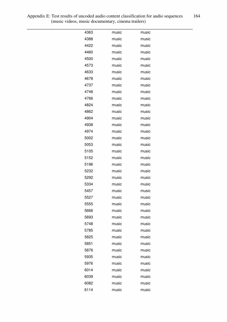
Appendix E: Test results of uncoded audio content classification for audio sequences (music videos, music documentary, cinema trailers) ______________________________________________________________
164
4363 music music
4388 music music
4422 music music
4460 music music
4500 music music
4573 music music
4633 music music
4678 music music
4737 music music
4748 music music
4766 music music
4824 music music
4862 music music
4904 music music
4938 music music
4974 music music
5002 music music
5053 music music
5105 music music
5152 music music
5196 music music
5232 music music
5292 music music
5334 music music
5457 music music
5527 music music
5555 music music
5666 music music
5693 music music
5748 music music
5785 music music
5825 music music
5851 music music
5876 music music
5935 music music
5976 music music
6014 music music
6039 music music
6082 music music
6114 music music
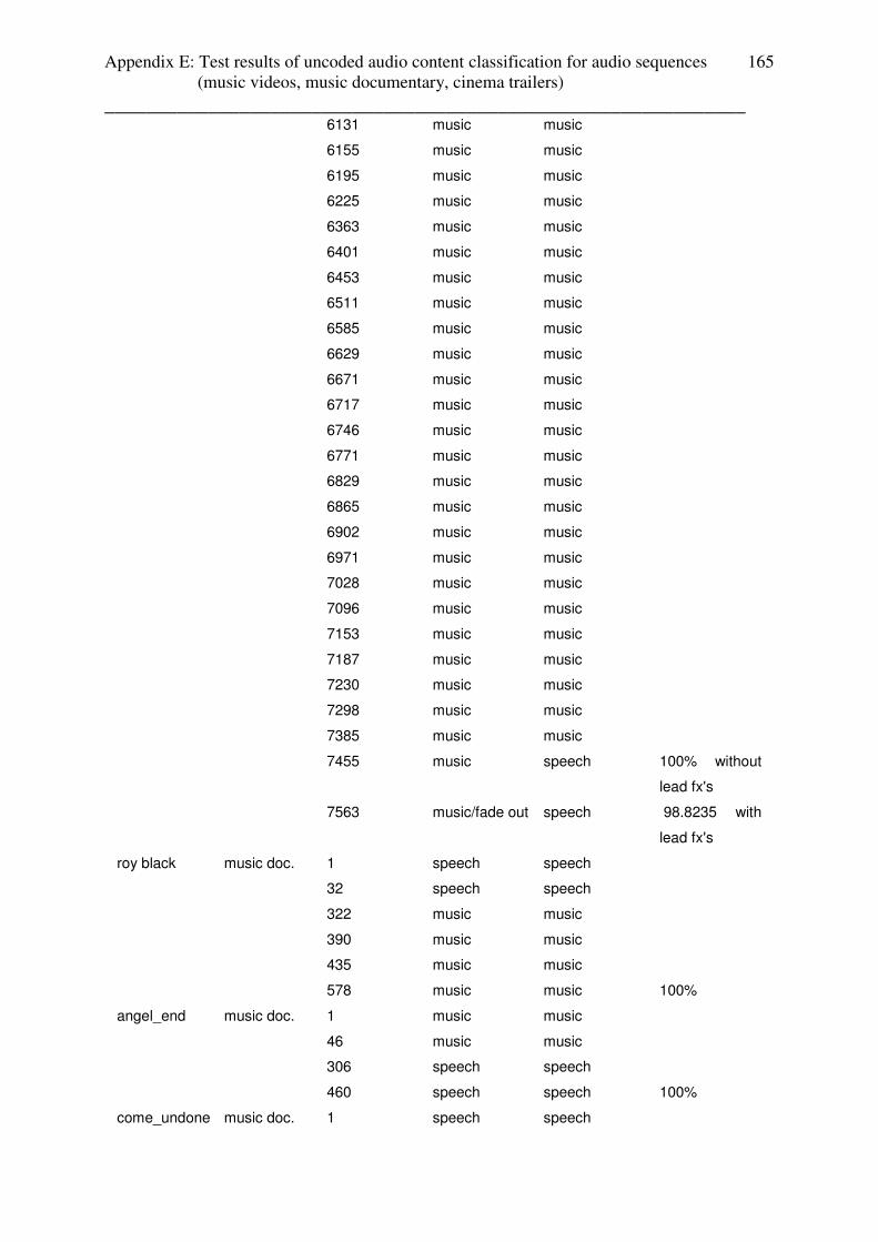
Appendix E: Test results of uncoded audio content classification for audio sequences (music videos, music documentary, cinema trailers) ______________________________________________________________
165
6131 music music
6155 music music
6195 music music
6225 music music
6363 music music
6401 music music
6453 music music
6511 music music
6585 music music
6629 music music
6671 music music
6717 music music
6746 music music
6771 music music
6829 music music
6865 music music
6902 music music
6971 music music
7028 music music
7096 music music
7153 music music
7187 music music
7230 music music
7298 music music
7385 music music
7455 music speech 100% without
lead fx's
7563 music/fade out speech 98.8235 with
lead fx's
roy black music doc. 1 speech speech
32 speech speech
322 music music
390 music music
435 music music
578 music music 100%
angel_end music doc. 1 music music
46 music music
306 speech speech
460 speech speech 100%
come_undone music doc. 1 speech speech

Appendix E: Test results of uncoded audio content classification for audio sequences (music videos, music documentary, cinema trailers) ______________________________________________________________
166
153 speech speech
406 music music
425 music music
585 speech speech
645 speech speech
675 speech music
704 speech speech
764 speech speech 89%
angel_start music doc. 1 speech speech
91 music speech
150 music music
210 music music
280 music music
300 music music
324 speech speech
349 music music
369 music music
387 music music 90%
joe black cinema trailer 1 silence music
20 music / fade in speech
80 music music
94 music music
127 music music
160 music music
191 music music
209 music music
245 music music
268 music music
354 music music
408 music music
453 music music
485 music music
514 music music
561 music music
594 music music
649 music music
676 music music
695 music music
709 music music
742 music music

Appendix E: Test results of uncoded audio content classification for audio sequences (music videos, music documentary, cinema trailers) ______________________________________________________________
167
756 music music
795 music music
821 music music
869 music music
937 music music
981 music music
1082 music speech
1137 music speech
1217 music speech
1316 music music
1366 music music
1418 music music
1451 music music
1485 music music
1534 music music
1578 music music
1647 music music
1699 music music
1775 music music
1807 music music
1841 music music
1915 music music
1982 music music
2013 music speech
2048 music music
2113 music music
2220 music music
2253 music music
2331 music music
2377 music music
2420 music music
2447 music music
2477 music music
2496 music music
2527 music music
2555 music music
2584 music music
2616 music music
2644 music music
2675 music speech

Appendix E: Test results of uncoded audio content classification for audio sequences (music videos, music documentary, cinema trailers) ______________________________________________________________
168
2712 music speech
2741 music music
2776 music music
2814 music music
2832 music music
2874 speech speech
2903 speech speech
2932 music speech
2962 music music
2996 music music
3024 music music
3049 music music
3119 music music
3146 music music
3180 music music
3237 music music
3264 music music
3304 music music
3319 music music
3354 music music
3378 music music
3430 music music
3464 music music
3509 music music
3545 music music
3593 music music
3620 music music
3659 music music
3689 music music
3725 music music
3747 music music
3791 music music
3814 music music
3852 music music
3887 music music
3933 music music
3965 music music
4004 music music
4038 music music
4076 music music

Appendix E: Test results of uncoded audio content classification for audio sequences (music videos, music documentary, cinema trailers) ______________________________________________________________
169
4088 music music
4104 music music
4132 music music
4152 music music
4202 music music
4249 music music
4419 music music
4567 music music
4604 music music
4687 music music
4718 music music
4875 music music
4928 music music
4991 music music
5086 music music
5250 music music
5284 music music 94.8276 with-
out lead fx's
5335 music/fade out speech 92.437 with
lead fx's
das spiel cinema trailer 1 music music
5 music music
37 music music
47 music music
94 music music
143 music music
193 music music
245 music music
263 music music
307 music music
339 music music
402 music music
432 music music
472 music music
488 music music
520 music music
555 music music
580 music music
599 music music
610 music music
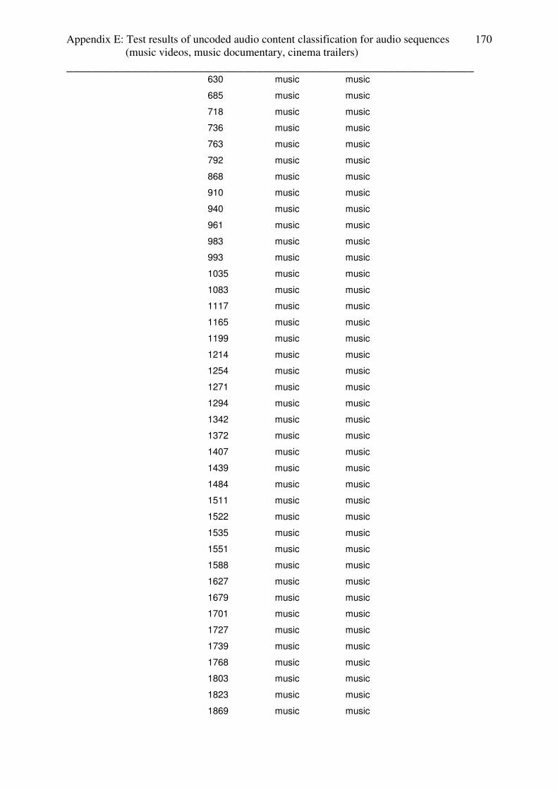
Appendix E: Test results of uncoded audio content classification for audio sequences (music videos, music documentary, cinema trailers) ______________________________________________________________
170
630 music music
685 music music
718 music music
736 music music
763 music music
792 music music
868 music music
910 music music
940 music music
961 music music
983 music music
993 music music
1035 music music
1083 music music
1117 music music
1165 music music
1199 music music
1214 music music
1254 music music
1271 music music
1294 music music
1342 music music
1372 music music
1407 music music
1439 music music
1484 music music
1511 music music
1522 music music
1535 music music
1551 music music
1588 music music
1627 music music
1679 music music
1701 music music
1727 music music
1739 music music
1768 music music
1803 music music
1823 music music
1869 music music
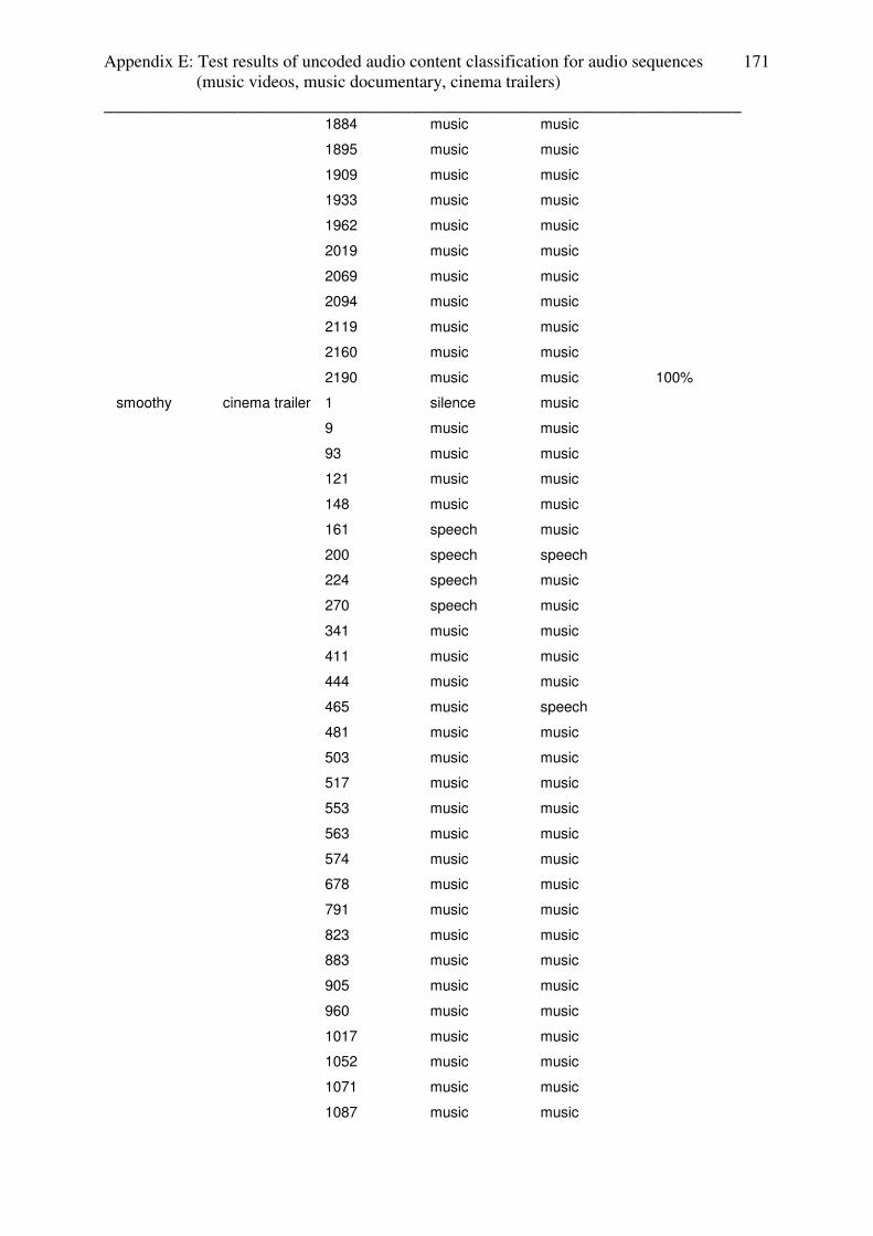
Appendix E: Test results of uncoded audio content classification for audio sequences (music videos, music documentary, cinema trailers) ______________________________________________________________
171
1884 music music
1895 music music
1909 music music
1933 music music
1962 music music
2019 music music
2069 music music
2094 music music
2119 music music
2160 music music
2190 music music 100%
smoothy cinema trailer 1 silence music
9 music music
93 music music
121 music music
148 music music
161 speech music
200 speech speech
224 speech music
270 speech music
341 music music
411 music music
444 music music
465 music speech
481 music music
503 music music
517 music music
553 music music
563 music music
574 music music
678 music music
791 music music
823 music music
883 music music
905 music music
960 music music
1017 music music
1052 music music
1071 music music
1087 music music

Appendix E: Test results of uncoded audio content classification for audio sequences (music videos, music documentary, cinema trailers) ______________________________________________________________
172
1125 music music
1209 music music
1229 music music
1248 music music
1280 music music
1287 music music
1307 music music
1350 music music
1385 music music
1424 music music
1448 music music
1463 music music
1488 music music
1515 music music
1569 music music
1606 music music
1650 music music
1662 music music
1691 speech speech
1752 music music
1783 speech music
1829 speech speech
1854 music music
1878 music music
1902 music music
1973 music music
2025 music music
2067 music music
2085 music music
2108 music music
2139 music music
2170 music music
2192 music music
2263 music music
2320 music music
2350 music music
2373 music music
2417 music music
2441 music music
2469 music music
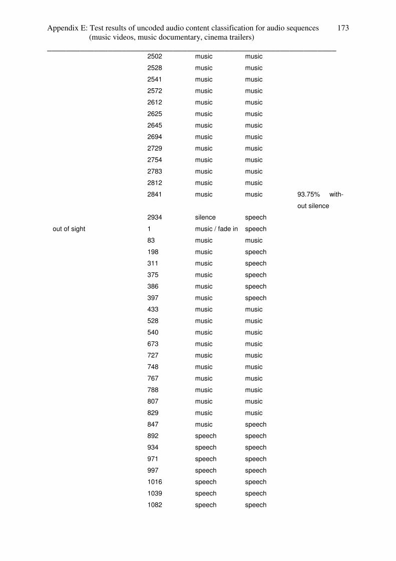
Appendix E: Test results of uncoded audio content classification for audio sequences (music videos, music documentary, cinema trailers) ______________________________________________________________
173
2502 music music
2528 music music
2541 music music
2572 music music
2612 music music
2625 music music
2645 music music
2694 music music
2729 music music
2754 music music
2783 music music
2812 music music
2841 music music 93.75% with-
out silence
2934 silence speech
out of sight 1 music / fade in speech
83 music music
198 music speech
311 music speech
375 music speech
386 music speech
397 music speech
433 music music
528 music music
540 music music
673 music music
727 music music
748 music music
767 music music
788 music music
807 music music
829 music music
847 music speech
892 speech speech
934 speech speech
971 speech speech
997 speech speech
1016 speech speech
1039 speech speech
1082 speech speech

Appendix E: Test results of uncoded audio content classification for audio sequences (music videos, music documentary, cinema trailers) ______________________________________________________________
174
1102 music music
1142 music music
1161 music music
1177 music music
1201 music music
1213 music music
1223 music music
1243 music music
1254 music music
1264 music music
1291 music music
1304 music music
1333 music music
1343 speech speech
1353 speech speech
1371 music music
1381 music music
1389 music music
1398 music music
1420 music music
1432 speech speech
1447 music music
1599 music music
1686 music music
1764 music music
1808 music music
1821 music music
1833 music music
1859 music music
1881 music music
1904 music music
1919 speech speech
1933 speech speech
1960 speech speech
1974 music music
1987 music music
2034 music music
2061 music music
2117 music music
2139 music music

Appendix E: Test results of uncoded audio content classification for audio sequences (music videos, music documentary, cinema trailers) ______________________________________________________________
175
2168 music music
2188 music music
2198 music music
2213 music music
2228 music music
2239 music music
2267 music music
2304 music music
2318 music music
2356 music music
2376 music music
2400 music music
2419 music music
2439 music music
2471 music music
2493 music music
2505 music music
2519 music music
2541 music music
2558 music music
2577 music speech
2616 music music
2637 music music
2725 music music
2869 music music
2979 music music 92.135% with-
out lead fx's
3210 music/fade out speech
pluto nash 1 music/fade in speech
105 music music
350 music music
397 music music
580 music music
631 music music
679 music music
696 music music
742 music music
764 music music
782 music music
800 music music
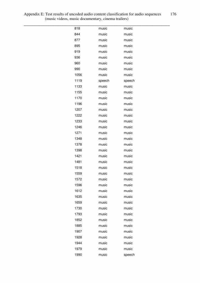
Appendix E: Test results of uncoded audio content classification for audio sequences (music videos, music documentary, cinema trailers) ______________________________________________________________
176
818 music music
844 music music
877 music music
895 music music
919 music music
936 music music
960 music music
990 music music
1056 music music
1119 speech speech
1133 music music
1155 music music
1170 music music
1196 music music
1207 music music
1222 music music
1233 music music
1246 music music
1271 music music
1348 music music
1378 music music
1398 music music
1421 music music
1481 music music
1518 music music
1559 music music
1572 music music
1596 music music
1612 music music
1635 music music
1659 music music
1730 music music
1793 music music
1852 music music
1885 music music
1907 music music
1928 music music
1944 music music
1979 music music
1990 music speech

Appendix E: Test results of uncoded audio content classification for audio sequences (music videos, music documentary, cinema trailers) ______________________________________________________________
177
2048 speech speech
2109 speech speech
2181 speech speech
2239 speech speech
2274 speech speech
2288 music music
2307 music music 98.2456% with-
out lead fx's
matrix_usa cinema trailer 1 music music
58 music music
132 music music
139 music music
218 music music
233 music music
252 music music
282 music music
293 music music
308 music music
344 music music
425 music music
464 music music
525 music music
538 music music
562 music music
577 music music
607 music music
633 music music
662 music music
679 music music
693 music music
703 music music
713 music music
732 music music
764 music music
779 music music
793 music music
819 music music
845 music music
858 music music
870 music music
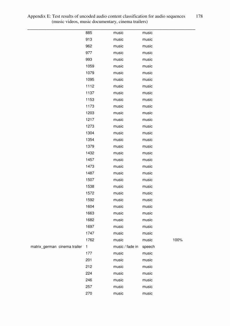
Appendix E: Test results of uncoded audio content classification for audio sequences (music videos, music documentary, cinema trailers) ______________________________________________________________
178
885 music music
913 music music
962 music music
977 music music
993 music music
1059 music music
1079 music music
1095 music music
1112 music music
1137 music music
1153 music music
1173 music music
1203 music music
1217 music music
1273 music music
1304 music music
1354 music music
1379 music music
1432 music music
1457 music music
1473 music music
1487 music music
1507 music music
1538 music music
1572 music music
1592 music music
1604 music music
1663 music music
1682 music music
1697 music music
1747 music music
1762 music music 100%
matrix_german cinema trailer 1 music / fade in speech
177 music music
201 music music
212 music music
224 music music
246 music music
257 music music
270 music music
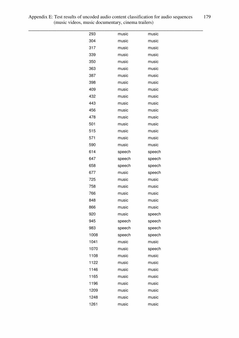
Appendix E: Test results of uncoded audio content classification for audio sequences (music videos, music documentary, cinema trailers) ______________________________________________________________
179
293 music music
304 music music
317 music music
339 music music
350 music music
363 music music
387 music music
398 music music
409 music music
432 music music
443 music music
456 music music
478 music music
501 music music
515 music music
571 music music
590 music music
614 speech speech
647 speech speech
658 speech speech
677 music speech
725 music music
758 music music
766 music music
848 music music
866 music music
920 music speech
945 speech speech
983 speech speech
1008 speech speech
1041 music music
1070 music speech
1108 music music
1122 music music
1146 music music
1165 music music
1196 music music
1209 music music
1248 music music
1261 music music
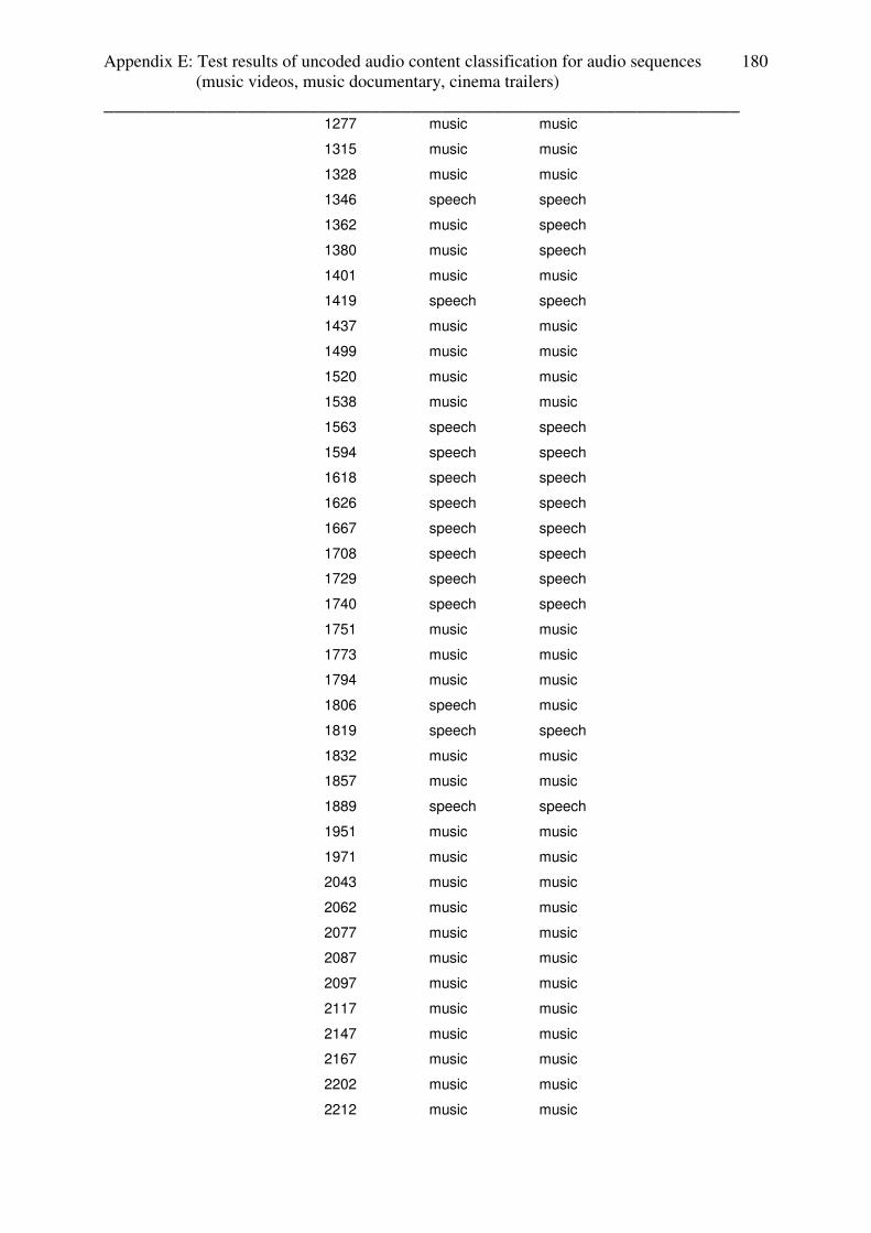
Appendix E: Test results of uncoded audio content classification for audio sequences (music videos, music documentary, cinema trailers) ______________________________________________________________
180
1277 music music
1315 music music
1328 music music
1346 speech speech
1362 music speech
1380 music speech
1401 music music
1419 speech speech
1437 music music
1499 music music
1520 music music
1538 music music
1563 speech speech
1594 speech speech
1618 speech speech
1626 speech speech
1667 speech speech
1708 speech speech
1729 speech speech
1740 speech speech
1751 music music
1773 music music
1794 music music
1806 speech music
1819 speech speech
1832 music music
1857 music music
1889 speech speech
1951 music music
1971 music music
2043 music music
2062 music music
2077 music music
2087 music music
2097 music music
2117 music music
2147 music music
2167 music music
2202 music music
2212 music music
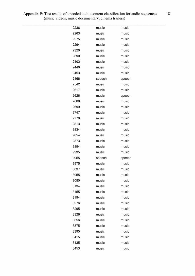
Appendix E: Test results of uncoded audio content classification for audio sequences (music videos, music documentary, cinema trailers) ______________________________________________________________
181
2236 music music
2263 music music
2275 music music
2294 music music
2320 music music
2390 music music
2402 music music
2440 music music
2453 music music
2466 speech speech
2542 music music
2617 music music
2626 music speech
2688 music music
2699 music music
2747 music music
2770 music music
2813 music music
2834 music music
2854 music music
2873 music music
2894 music music
2935 music music
2955 speech speech
2975 music music
3037 music music
3055 music music
3080 music music
3134 music music
3155 music music
3194 music music
3276 music music
3295 music music
3326 music music
3356 music music
3375 music music
3395 music music
3415 music music
3435 music music
3453 music music
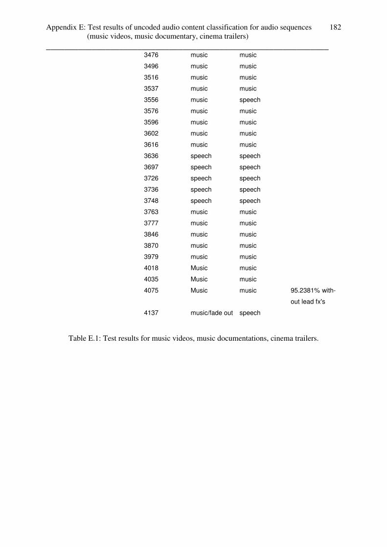
Appendix E: Test results of uncoded audio content classification for audio sequences (music videos, music documentary, cinema trailers) ______________________________________________________________
182
3476 music music
3496 music music
3516 music music
3537 music music
3556 music speech
3576 music music
3596 music music
3602 music music
3616 music music
3636 speech speech
3697 speech speech
3726 speech speech
3736 speech speech
3748 speech speech
3763 music music
3777 music music
3846 music music
3870 music music
3979 music music
4018 Music music
4035 Music music
4075 Music music 95.2381% with-
out lead fx's
4137 music/fade out speech
Table E.1: Test results for music videos, music documentations, cinema trailers.
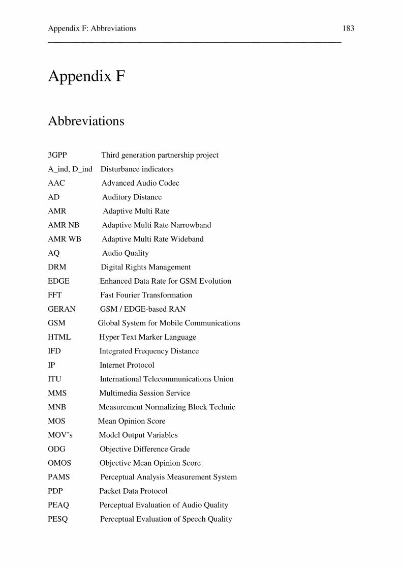
Appendix F: Abbreviations ______________________________________________________________
183
Appendix F
Abbreviations
3GPP Third generation partnership project
A_ind, D_ind Disturbance indicators
AAC Advanced Audio Codec
AD Auditory Distance
AMR Adaptive Multi Rate
AMR NB Adaptive Multi Rate Narrowband
AMR WB Adaptive Multi Rate Wideband
AQ Audio Quality
DRM Digital Rights Management
EDGE Enhanced Data Rate for GSM Evolution
FFT Fast Fourier Transformation
GERAN GSM / EDGE-based RAN
GSM Global System for Mobile Communications
HTML Hyper Text Marker Language
IFD Integrated Frequency Distance
IP Internet Protocol
ITU International Telecommunications Union
MMS Multimedia Session Service
MNB Measurement Normalizing Block Technic
MOS Mean Opinion Score
MOV’s Model Output Variables
ODG Objective Difference Grade
OMOS Objective Mean Opinion Score
PAMS Perceptual Analysis Measurement System
PDP Packet Data Protocol
PEAQ Perceptual Evaluation of Audio Quality
PESQ Perceptual Evaluation of Speech Quality
Appendix F: Abbreviations ______________________________________________________________
184
PSQM Perceptual Speech Quality Measurement
PSQM+ Advanced Speech Quality Measurement
PSS Packet Switched Streaming Service
QoS Quality of Service
RFC IETF Request For Comments
RTSP Real Time Streaming Protocol
SDP Session Description Protocol
UMTS Universal Mobile Telecommunications System
URI Universal Resource Identifier
UTRAN UMTS Radio Access Network
VoIP Voice over IP
VQEP Video Quality Expert Group
WAP Wireless Application Protocol
WWW World Wide Web
ZCR Zero Crossing Rate
Bibliography ______________________________________________________________
185
Bibliography
[1] M. Ries, R. Puglia, T. Tebaldi, O. Nemethova, M. Rupp, “Audiovisual Quality
Estimation for Mobile Streaming Services,”, Proc. Of International Symposium on
Wireless Communication Systems IEEE Ed., Sept, 2005
[2] R. Puglia, “Influence of Audio and Video Quality on Subjective Audiovisual Quality,
H.263 and Adaptive Multi Rate (AMR) coding,”, Diploma Thesis, Institute for radio
frequency and communication engineering, 2005
[3] T. Tebaldi, “Influence of Audio and Video Quality on Subjective Audiovisual Quality,
MPEG-4 and AAC,”, Diploma Thesis, Institute for radio frequency and communication
engineering, 2005
[4] S. Winkler, C. Faller, “Audiovisual Quality Evaluation of Low-Bitrate Video,”, Proc.
IS&T/SPIE International Symposium Electronic Imaging, San Jose, CA, USA, vol. 5666,
Jan. 2005
[5] S. Winkler, C. Faller, “Maximizing Audiovisual Quality at Low Bitrates,”,
[6] Brandenburg K., “Evaluation of Quality for Audio Encoding at low Bit Rates,” 82nd AES
Convention, London 1987, Preprint #2433
[7] ITU-R Recommendation BS 1387, “Method for Objective Measurements of Perceived
Audio Quality (PEAQ),”, 1998
[8] Adrian E. Conway, Yali Zhu, “Applying Objective Perceptual Quality Assessment
Methods in Network Performance Modelling”
[9] A. W. Rix, M. P. Hollier, “ The perceptual analysis measurement system for robust
end-to-end speech quality assessment,” IEEE ICASSP ’00 Proceedings, Vol.3,
pp. 1515 – 1518, 2000
Bibliography ______________________________________________________________
186
[10] ITU-T Contribution COM 12-20-E, “Improvement of the P.861
Perceptual Speech Quality Measure,”, KPN research, Netherlands, Dec. 1997
[11] ITU-T Recommendation P.862, “Perceptual evaluation of speech quality (PESQ), an
objective method for end-to-end speech quality assessment of narrowband telephone
networks and speech codecs,”, 2001
[12] Opticom Instruments, “Voice Quality Testing for Wireless Networks,”
[13] Voran, S., “ Objective estimation of perceived speech quality – Part 1: Development of
the measuring normalizing block technique,”, IEEE Transactions on Speech and Audio
Processing, 1999
[14] A.W.Rix, J. G. Beerends, M.P. Hollier, A.P. Hekstra, “Perceptual Evaluation of Speech Quality (PESQ) – A new method for Speech Quality Assessment of telephone networks and codecs,”
[15] Zwicker E., Feldtkeller R., “Das Ohr als Nachrichtenempfänger”, Hirzel-Verlag,
Stuttgart, 1967
[16] Zwicker E., „Psychoakustik,“, Springer-Verlag, Berlin-Heidelberg-New York, 1982
[17] Zwicker, E., H. Fastl, “Psychoacoustics, Facts and Models (2 ed.),”, Volume 22 of
Series of Information Sciences, Berlin: Springer.
[18] P. Corriveau, A. Webster, A. Rohaly, J. Libert, “Video Quality Experts Group: the quest
for valid objective methods,” in Proc. SPIE vol. 3959, Human Vision and Electronic
Imaging V, B. Rogowitz, and T. Pappas, Eds., pp. 129-139, June 2000
[19] A. Rohlay et al, “Video Quality Experts Group: current results and future directions,” in
Proc. SPIE vol. 4067, Visual Communications and Image Processing 2000, K. Ngan, T.
Sikora, and M. Sun, Eds., pp. 742-753, May 2000

Bibliography ______________________________________________________________
187
[20] Y. Wang, Z. Liu, and J-C Huang, “Multimedia Content Analysis”, IEEE Signal
Processing Magazine, IEEE 2000
[21] G.Lu, T. Hankinson, ”An Investigation of Automatic Audio Classification and
Segmentation,”, Proceedings of ICSP 2000
[22] T. Zhang, C.-C. Jay Kue, “Audio Content Analysis for Online Audiovisual Data
Segmentation and Classification,”, IEEE Transactions on speech and audio processing,
Vol. 9, No. 4, May 2001
[23] K. Melih, R. Gonzalez, ”Audio Source Type Segmentation using a Perceptually based
Representation,”, Fifth International Symposium on Signal Processing and its
Applications, ISSPA #99, Brisbane, Australia, 22-25 August 1999, Organised by the
Signal Processing Research Centre, QUT, Brisbane, Australia
[24] M. Liu, C. Wan, “ A Study on Content-Based Classification and Retrieval of Audio
Database,”, IEEE 2001
[25] M. Abe, J. Masumoto, and M. Nishiguchi, “Content-Based Classification of Audio
Signals using Source and Structure Modelling,”
[26] A. Rauber, E. Pampalk, D. Merkl, “ The SOM-enhanced JukeBox: Organization and
Visualization of Music Collections based on Perceptual Models”
[27] Y. Wang, J. Huang, Z. Liu, T. Chen, „Multimedia Content Classification using Motion
and Audio Infomation“, IEEE International Symposium on Circuits and Systems, June
9-12, 1997, Hong Kong
[28] L. Lu, H.J. Zhang, S.Z. Li, “Content-based audio classification and segmentation by
using support vector machines,”, Multimedia Systems 8: 482 – 492, 2003

Bibliography ______________________________________________________________
188
[29] S. J. Rizvi, L. Chen, M. T. Özsu, “MADClassifier: Content-Based Continous
Classification of Mixed Audio Data”, Technical Report CS-2002-34 October 2002,
School Of Computer Science, University of Waterloo, Waterlo, ON
[30] P. J. Moreno, R. Rifkin, “Using the Fisher Kernel Method for Web Audio
Classification,” Technical Paper from Compaq Computer Corporation Cambridge
Research Laboratory One Kendall Square, Building 700 Cambridge, Massacgusetts
02139 United States, 2000 IEEE
[31] A. Rauber, E. Pampalk, D. Merkl, „Using psycho-acoustic models and self-organizing
maps to create a hierarchical structuring of music by musical styles,“ in Proc. Of the 3rd
International Conference on Music Information Retrieval, pp. 71-80, October 13-17,
2002, Paris, France
[32] TeliaSonera, MediaLab, ” Packet Switched Streaming Service,”, White Paper, 2003
[33] 3GPP TS 26.233: 3rd Generation Partnership Project; Technical Specification Group
Services and System Aspects; Transparent end-to-end packet switched streaming service
(PSS); General Description (Release 6)
[34] 3GPP TS 26.244: 3rd Generation Partnership Project; Technical Specification Group
Services and System Aspects; Transparent end-to-end packet switched streaming service
(PSS); 3GPP file format (3GP) (Release 6)
[35] IETF RFC 1889: “Real-Time Transport Protocol,”
[36] IETF RFC 3267, “RTP payload format and file storage format for the Adaptive Multi-
Rate (AMR) Adaptive Multi-Rate Wideband (AMR-WB) audio codecs”, March 2002
[37] F. Ghys, M. Mampaey, M. Smouts, A. Vaaraniemi, “3G Multimdia network services,
accounting, and user profiles,”, Artech House mobile communication series, 2003

Bibliography ______________________________________________________________
189
[38] Y. Kikuchi. et al., “RTP Payload Format for MPEG-4 Audio/Visual Streams,”, IETF
RFC 3016, November 2000
[39] C. Bormann et al., “RTP Payload Format for 1998 Version of ITU-T Rec. H.263 Video
(H.263+),”, IETF RFC 2429, October 1998
[40] H. Schulzrinne, A. Rao, R. Lanphier, “Real Time Streaming Protocol (RTSP),”, IETF
RFC 2326, April 1998
[41] 3GPP TS 26.234: 3rd Generation Partnership Project; Technical Specification Group
Services and System Aspects; Transparent end-to-end packet switched streaming service
(PSS); Protocol and codecs (Release 6)
[42] H. Schulzrinne, et al, ”RTP: A Transport Protocol for Real-Time Applications,”, IETF
RFC 1889, January 1996
[43] 3GPP TS 23.107: 3rd Generation Partnership Project; Technical Specification Group
Services and System Aspects; Quality of Service (QoS) concept and architecture
(Release 6)
[44] Etoh, ”Next Generation Mobile Systems,”, John Wiley & Sons, Ltd, 2005
[45] D. J. M. Robinson, M. J. Hawksford, “Time-Domain Auditory Model for the
Assessment of High-Quality Coded Audio,”
[46] Y.A. Huang, J. Benesty, “Audio Signal Processing for Next-Generation Multimedia
Communication System,”, Kluwer Academic Publishers, 2004].
[47] R. Jourdain, “Das wohltemperierte Gehirn: Wie Musik im Kopf entsteht und wirkt,”,
Spektrum Akademischer Verlag, 2001
[48] T. Painter, A. Spanias, “ Perceptual Coding of Digital Audio,“, Proceedings of the IEEE,
Vol. 88, No. 4, April 2000

Bibliography ______________________________________________________________
190
[49] T. C. Justus, J. J. Bharucha, “Music perception and cognition,”, Stevens Handbook of
Experimental Psychology Volume 1: Sensation and Perception (Third Edition, pp. 453-
492), New York: Wiley, 2002
[50] T. Painter, A. Spanias, “ Perceptual Coding of Digital Audio,“, Proceedings of the IEEE,
Vol. 88, No. 4, April 2000
[51] U. Zölzer, “Digitale Audiosignalverarbeitung,”, B. G. Teubner Verlag / GWV
Fachverlage GmbH, Wiesbaden, 2005