Embed Size (px)
Citation preview

Draft version September 30, 2018Preprint typeset using LATEX style emulateapj v. 5/2/11
THE GIANT MOLECULAR CLOUD ENVIRONMENTS OF INFRARED DARK CLOUDS
Audra K. HernandezDepartment of Astronomy, University of Wisconsin, 475 North Charter Street, Madison, WI 53706, USA;
Jonathan C. TanDepartments of Astronomy & Physics, University of Florida, Gainesville, FL 32611, USA;
Draft version September 30, 2018
ABSTRACT
We study Giant Molecular Cloud (GMC) environments surrounding 10 Infrared Dark Clouds(IRDCs), using 13CO(1− 0) emission from the Galactic Ring Survey. We measure physical propertiesof these IRDCs/GMCs on a range of scales extending to radii, R, of 30 pc. By comparing differentmethods for defining cloud boundaries and for deriving mass surface densities and velocity dispersions,we settle on a preferred “CE,τ ,G” method of “Connected Extraction” in position-velocity space plusGaussian fitting to opacity-corrected line profiles for velocity dispersion and mass estimation. Weexamine how cloud definition affects measurements of the magnitude and direction of line-of-sightvelocity gradients and velocity dispersions, including associated dependencies on size scale. CE,τ ,G-defined GMCs show velocity dispersion versus size relations σ ∝ s1/2, which are consistent with thelarge-scale gradients being caused by turbulence. However, IRDCs have velocity dispersions thatare moderately enhanced above those predicted by this scaling relation. We examine the dynamicalstate of the clouds finding mean virial parameters αvir ' 1.0 for GMCs and 1.6 for IRDCs, broadlyconsistent with models of magnetized virialized pressure-confined polytropic clouds, but potentiallyindicating that IRDCs have more disturbed kinematics. CE,τ ,G-defined clouds exhibit a tight corre-lation of σ/R1/2 ∝ Σn, with n ' 0.7 for GMCs and 1.3 for IRDCs (c.f., a value of 0.5 expected for apopulation of virialized clouds). We conclude that while GMCs show evidence for virialization overa range of scales, IRDCs may be moderately super virial. Alternatively, IRDCs could be virializedbut have systematically different 13CO gas phase abundances, i.e., due to freeze-out, affecting massestimations.Subject headings: ISM: clouds - ISM: kinematics and dynamics - Stars: formation
1. INTRODUCTION
Galactic star formation resides mostly within Giant Molecular Clouds (GMCs), conventionally defined to have masses≥ 104 M and observed to extend up to several ×106 M (e.g., Blitz 1993; Williams et al. 2000; McKee & Ostriker2007). With typical mass surface densities of ∼ 100M pc−2, GMCs have mean radial sizes of ∼ 6− 100 pc, assumingsimple circular symmetry. However, GMCs are highly irregular and hierarchical structures. Their dense clumps canspawn stellar clusters and associations, creating the bulk of the Galactic field star population. The efficiency and rateof star formation from these clumps is relatively low, i.e., a few percent per local free-fall time (Zuckerman & Evans1974; Krumholz & Tan 2007). This appears to be mostly because much of the GMC material is stable with respect togravitational collapse, especially material below a threshold AV ∼ 10 mag (e.g., Lada et al. 2010). Higher total starformation efficiencies, ∼ 10 − 50%, appear to be possible in the star-forming clumps that form at least moderatelybound clusters (Lada & Lada 2003).
Different theoretical models of the processes that create star-forming clumps within GMCs or prevent overdensities inthe bulk of the cloud are actively debated. These processes include the regulation of star formation and stabilization ofgas by magnetic fields (McKee 1989; Mouschovias 2001) or turbulence (Krumholz & McKee 2005; Padoan & Nordlund2011), and/or the initiation of star formation by discrete triggering events, such as converging atomic flows (e.g.,Heitsch et al. 2006), cloud collisions (e.g., Tan 2000) or stellar feedback (e.g., Samal et al. 2014).
Infrared dark clouds (IRDCs) are likely to be examples of early stage star-forming clumps (e.g., Perault et al. 1996;Egan et al. 1998; Carey et al. 2000; Rathborne et al. 2006; Butler & Tan 2009; Peretto & Fuller 2009; Battersby et al.2010). Thus their study may help us understand the processes that initiate star formation in GMCs. There have beenmany investigations of the internal properties of IRDCs, including their temperatures (e.g., Pillai et al. 2006; Perettoet al. 2010; Ragan et al. 2011; Chira et al. 2013), mass surface density structure (e.g., Butler & Tan 2009; Peretto& Fuller 2009; Ragan et al. 2011; Butler & Tan 2012; Kainulainen & Tan 2013; Butler et al. 2014), kinematics (e.g.,Henshaw et al. 2013; Jimenez-Serra et al. 2014) and dynamics (e.g., Hernandez & Tan 2011; Hernandez et al. 2012),CO depletion (Fontani et al. 2006; Hernandez et al. 2011), chemistry (Sanhueza et al. 2013). See Tan et al. (2014) fora review.
However, there have been fewer studies connecting IRDCs to their larger-scale environments, such as the morphology,
arX
iv:1
502.
0018
3v3
[as
tro-
ph.G
A]
18
Jun
2015

2
kinematics and dynamics of their parent clouds. Theories involving production of dense gas in shocks have beensupported by detection of large-scale SiO emission along IRDCs (Jimenez-Serra et al. 2010; Nguyen-Lu’o’ng et al.2013). However, these studies focus only on a few individual clouds and are still confined to a few-parsec scales in andaround the filamentary molecular clouds.
Here we study the 13CO(1-0)-emitting gas in and around 10 well-studied IRDCs, utilizing data from the BU-FCRAOGalactic Ring Survey (GRS; Jackson et al. 2006). We consider a range of scales out to 30 pc projected radius, expectedto encompass the potential GMC environment of the IRDC. While our study connects to scales typical of other large-sample GMC studies (e.g., Heyer et al. 2009; Roman-Duval et al. 2009, 2010), by focusing on just 10 regions we areable to investigate their kinematic properties in much greater detail. Other studies done on such a range of scales,from clump to GMCs, have been performed on nearby GMCs, such as Orion A (e.g., Shimajiri et al. 2011), Taurus(e.g., Goldsmith et al. 2008), and Perseus (Ridge et al. 2006; Foster et al. 2009; Kirk et al. 2010). However, these localGMCs do not seem to give rise to the more extreme range of star-forming clumps that is found in IRDCs.
The main focus of this paper is to “bridge the gap” between IRDC and GMC studies. The questions we aim toaddress include: Are IRDCs typically found within GMCs? Are IRDCs found within specific locations with respect toGMCs? Are IRDCs and their surrounding GMCs virialized, and does their degree of virialization vary as a functionof cloud physical scale?
The IRDC/GMC sample is presented in §2. Methods for defining cloud boundaries and estimating masses andkinematic properties are described in §3. Results are presented in §4, including derived physical properties of theclouds (§4.1), the location of IRDCs within their respective GMCs (§4.2), and the kinematic and dynamical analysisof the IRDC and GMCs (§4.3). We conclude in §5.
2. THE IRDC SAMPLE AND MOLECULAR LINE DATA
We utilize the 13CO(J = 1→ 0) data of the GRS survey (Jackson et al. 2006), which covers 18 ≤ l ≤ 56, b±1 and−5 < vLSR < 135 km s−1 (for l ≤ 40) and −5 < vLSR < 85 km s−1 (for l ≥ 40). The GRS had a spatial resolutionof 46′′, with 22′′ sampling, and a spectral resolution of 0.212 km s−1. The typical rms noise is σ(T∗A) = 0.13 K (orσ(TB,ν) ∼ 0.26 K with a main beam efficiency of 0.48).
Our selected IRDCs are the 10 clouds from Butler & Tan (2009, hereafter BT09) (see also Butler & Tan 2012;Kainulainen & Tan 2013). This sample, a subset of that of Rathborne et al. (2006), was chosen while considering the8µm (IRAC band 4) images from the Spitzer Galactic Legacy Mid-Plane Survey Extraordinaire (GLIMPSE; Benjaminet al. 2003). These IRDCs were selected for being relatively nearby, massive, dark (i.e., relatively high contrast againstthe surrounding diffuse emission), and surrounded by relatively smooth diffuse emission within the 8µm GLIMPSEimages. Characteristic sizes and boundaries for each IRDC were taken from Simon et al. (2006a), where ellipses werefitted based on extinction in MSX images. Although these fitted ellipses are not necessarily accurate of IRDC shapes,they provide a convenient measure of the approximate cloud structure. The catalog coordinates and sizes for the 10IRDCs (including “single component” sub-classifications, labelled “-s”, see below) are listed in Table 1.
TABLE 1The IRDC Sample
IRDC lIRDCa bIRDC
a rmaja rmin
a PAea l0 b0 v0 l0,τ b0,τ v0,τ db Tex
c
() () (′) (′) () () () km s−1 () () km s−1 ( kpc) (K)
A 18.822 -0.285 14.1 3.90 74.0 18.850 -0.276 64.3 18.862 -0.276 64.5 4.80 8.90
B 19.271 0.074 8.40 1.80 88.0 19.287 0.075 26.5 19.287 0.075 26.7 2.40 7.11
C 28.373 0.076 12.0 9.30 78.0 28.370 0.062 79.0 28.364 0.062 79.2 5.00 7.86
D 28.531 -0.251 20.4 5.10 60.0 28.567 -0.233 78.6 28.567 -0.239 80.7 5.70 7.00
D-s 28.555 -0.251 87.9 28.549 -0.257 87.7
E 28.677 0.132 14.6 4.10 103 28.672 0.130 80.7 28.684 0.130 81.3 5.10 7.00
F 34.437 0.245 5.30 2.00 79.0 34.434 0.240 57.3 34.428 0.240 57.5 3.70 6.48
F-s 34.434 0.240 58.0 34.428 0.240 58.0
G 34.771 -0.557 6.60 2.00 95.0 34.764 -0.559 43.9 34.764 -0.559 44.1 2.90 8.69
G-s 34.770 -0.559 44.4 34.764 -0.559 44.4
H 35.395 -0.336 20.6 6.40 59.0 35.422 -0.319 47.5 35.416 -0.319 48.0 2.90 6.61
H-s 35.391 -0.337 43.9 35.391 -0.337 44.4
I 38.952 -0.475 7.50 3.00 64.0 38.942 -0.473 43.5 38.942 -0.473 43.2 2.70 7.24
J 53.116 0.054 1.60 1.30 50.0 53.114 0.056 21.4 53.120 0.056 21.6 1.80 7.05
aIRDC coordinates and elliptical sizes adopted from Simon et al. (2006a)bIRDC kinematic distances adopted from Rathborne et al. (2006)cThe 13CO excitation temperatures adopted from Roman-Duval et al. (2010)
Kinematic distances were adopted from Rathborne et al. (2006) and Simon et al. (2006b), where the IRDC centralvelocity was matched morphologically between the mid-infrared (MIR) extinction estimated from MSX and the 13COemission from the GRS. These distances were estimated assuming the rotation curve of Clemens (1985). We assumeuncertainties of 20%, given the size of streaming motions of ∼ 10 − 20 km s−1 of clouds with trigonometric parallaxmeasurements (e.g., Brunthaler et al. 2009; Reid et al. 2014).
3
19.0 18.8 18.6l
−0.50
−0.25
0.00
b
19.0 18.8 18.6l
50
75
100
125
I [K
km
s−
1]
19.0 18.8 18.6l
50
55
60
65
70
75
vls
r (k
m s
−1)
−0.5 −0.2 0.0b
19.0 18.8 18.6l
−0.5 −0.2 0.0b
0.0
0.5
1.0
1.5
2.0
2.5
K d
eg
A
B
C
D
E
19.6 19.2 18.8l
−0.5
0.0
0.5
b
19.6 19.2 18.8l
60
80
100
120
140
I [K
km
s−
1]
19.6 19.2 18.8l
15
20
25
30
35
40
vls
r (k
m s
−1)
−0.5 0.0 0.5b
19.6 19.2 18.8l
−0.5 0.0 0.5b
0.0
0.5
1.0
1.5
2.0
K d
eg
A
B
C
D
E
28.6 28.4 28.2l
−0.25
0.00
0.25
b
28.6 28.4 28.2l
45
60
75
90
105
120
I [K
km
s−
1]
28.6 28.4 28.2l
65
70
75
80
85
90v
lsr (k
m s
−1)
−0.2 0.0 0.2b
28.6 28.4 28.2l
−0.2 0.0 0.2b
0.0
0.5
1.0
1.5
2.0
K d
eg
A
B
C
D
E
28.8 28.6 28.4l
−0.50
−0.25
0.00
b
28.8 28.6 28.4l
50
60
70
80
I [K
km
s−
1]
28.8 28.6 28.4l
65
70
75
80
85
90
vls
r (k
m s
−1)
−0.5 −0.2 0.0b
28.8 28.6 28.4l
−0.5 −0.2 0.0b
0.0
0.5
1.0
K d
eg
A
B
C
D
E
28.8 28.5l
0.00
0.25
b
28.8 28.5l
60
80
100
120
I [K
km
s−
1]
28.8 28.5l
70
75
80
85
90
95
vls
r (k
m s
−1)
0.0 0.2b
28.8 28.5l
0.0 0.2b
0.0
0.5
1.0
1.5
K d
eg
A
B
C
D
E
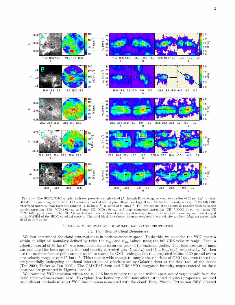
Fig. 1.— The IRDC/GMC sample: each row presents a single cloud (A through E) showing data out to a radius of 30 pc. Left to right:GLIMPSE 8 µm image with the IRDC boundary marked with a pink ellipse (see Figs. 3 and A1-A4 for intensity scales); 13CO(1-0) GRSintegrated intensity map (over the range v0 ± 15 km s−1) in units of K km s−1; Full projections of the cloud in position-velocity space:simple-extraction (SE) 13CO(1-0) vlsr vs l map, SE 13CO(1-0) vlsr vs b map; connected extraction (CE) 13CO(1-0) vlsr vs l map; CE13CO(1-0) vlsr vs b map. The IRDC is marked with a white box of width equal to the extent of the elliptical boundary and height equalto the FWHM of the IRDC co-added spectra. The solid black line shows the mass-weighted linear velocity gradient (dv0/ds) across eachcloud at R = 30 pc.
3. METHODS: DERIVATIONS OF MOLECULAR CLOUD PROPERTIES
3.1. Definition of Cloud Boundaries
We first determined the cloud center-of-mass in position-velocity space. To do this, we co-added the 13CO spectrawithin an elliptical boundary defined by twice the rmaj and rmin values, using the full GRS velocity range. Then, avelocity interval of 30 km s−1 was considered, centered on the peak of the emission profile. The cloud’s center-of-masswas evaluated for both optically thin and opacity corrected gas, (l0, b0, v0) and (l0,τ , b0,τ , v0,τ ), respectively. We thenuse this as the reference point around which to search for GMC-scale gas, out to a projected radius of 30 pc and over anew velocity range of v0± 15 km s−1. This range is wide enough to sample the velocities of GMC gas, even those thatare potentially undergoing collisional interactions at velocities set by Galactic shear at the tidal radii of the clouds(Tan 2000; Tasker & Tan 2009). The GLIMPSE 8µm and GRS 13CO integrated intensity maps centered on theselocations are presented in Figures 1 and 2.
We examined 13CO emission within the v0 ± 15 km/s velocity range and within apertures of varying radii from thecloud center-of-mass coordinate. To explore how boundary definitions affect estimated physical properties, we usedtwo different methods to select 13CO line emission associated with the cloud. First, “Simple Extraction (SE)” selected

4
34.8 34.5 34.2l
0.0
0.3
0.6
b
34.8 34.5 34.2l
3040
50
60
70
8090
I [K
km
s−
1]
34.8 34.5 34.2l
45
50
55
60
65
70
vls
r (k
m s
−1)
0.0 0.3 0.6b
34.8 34.5 34.2l
0.0 0.3 0.6b
0.0
0.5
1.0
1.5
K d
eg
F
G
H
I
J
35.0 34.5l
−1.0
−0.5
0.0
b
35.0 34.5l
30
40
50
60
I [K
km
s−
1]
35.0 34.5l
30
35
40
45
50
55
vls
r (k
m s
−1)
−1.0 −0.5 0.0b
35.0 34.5l
−1.0 −0.5 0.0b
0.0
0.5
1.0
1.5
2.0
K d
eg
F
G
H
I
J
35.7 35.4 35.1l
−0.9
−0.6
−0.3
0.0
b
35.7 35.4 35.1l
30
40
50
60
70
I [K
km
s−
1]
35.7 35.4 35.1l
35
40
45
50
55
60v
lsr (k
m s
−1)
−0.9 −0.6 −0.3 0.0b
35.7 35.4 35.1l
−0.9 −0.6 −0.3 0.0b
0.0
0.5
1.0
1.5
2.0
K d
eg
F
G
H
I
J
39.5 39.0 38.5l
−1.0
−0.5
0.0
b
39.5 39.0 38.5l
20
30
40
50
60
70
I [K
km
s−
1]
39.5 39.0 38.5l
30
35
40
45
50
55
vls
r (k
m s
−1)
−1.0 −0.5 0.0b
39.5 39.0 38.5l
−1.0 −0.5 0.0b
0.0
0.5
1.0
1.5
K d
eg
F
G
H
I
J
53.6 52.8l
−0.75
0.00
0.75
b
53.6 52.8l
15
20
25
30
I [K
km
s−
1]
53.6 52.8l
10
15
20
25
30
35
vls
r (k
m s
−1)
−0.8 0.0 0.8b
53.6 52.8l
−0.8 0.0 0.8b
0.00.51.01.52.02.53.03.54.0
K d
eg
F
G
H
I
J
Fig. 2.— The same as Figure 1, but for Clouds F through J.
all the 13CO emission within radii R = 5, 10, 20, and 30 pc and v0 ± 15 km/s. Second, “Connected Extraction (CE)”defined a cloud as a connected structure in l-b-v-space with all cloud voxels required to be above a given thresholdintensity: we defined a given voxel as “molecular cloud gas” if its 13CO(1-0) line intensity TB,ν ≥ 1.35 K (i.e., theGRS 5σrms noise level). The CE search was also limited to within a 30 pc radius and ±15 km s−1 of the IRDCcenter-of-mass. Position-velocity maps for each cloud, defined by both SE and CE, are shown in Figures 1 and 2.
Clouds defined by CE do not have simple radial sizes. Therefore, we estimated three circular boundaries, centeredon the extracted cloud’s center-of-mass: (1) mass-weighted radius, RM , defined as mean projected radial distance ofcloud mass from the center of mass; (2) areal radius, RA, defined by the total projected area A = πR2
A = NpAp, whereNp is the total number of pixels subtended by the cloud and Ap is the area of one image pixel; (3) half-mass radius,R1/2, defined as the radius from cloud center that contains half of the total mass.
For the IRDCs, we also selected “cloud” material via SE and CE using the spatial coordinates and elliptical bound-aries from Simon et al. (2006a), along with the v0 ± 15 km s−1 velocity intervals.
3.2. Column Densities and Masses from 13CO emission
We estimated the 13CO column density of each molecular cloud voxel, dN13CO from their J = 1 → 0 line emissionassuming a partition function with a thermal distribution described by an excitation temperature Tex via:
dN13CO
dv=
8πQrot
Aλ30
glgu
τν1− exp(−hν/[kTex])
, (1)

5
where Qrot is the partition function, A = 6.294 × 10⁻⁸s−1 is the Einstein coefficient, λ0 = 0.27204 cm, gl = 1 andgu = 3 are the statistical weights of the lower and upper levels and τν is the optical depth of the line at frequencyν, i.e., at velocity v. Each GRS voxel has a velocity width of dv = 0.212 km s−1. For linear molecules, the partitionfunction is Qrot =
∑∞J=0(2J + 1)exp(−EJ/kTex) with EJ = J(J + 1)hB where J is the rotational quantum number
and B = 5.5101× 10¹⁰ s−1 is the rotational constant. For 13CO(1-0) we have EJ/k = 5.289 K.Many studies of the physical properties of GMCs and IRDCs have accounted for line optical depth when estimating
their physical properties (e.g., Heyer et al. 2009; Roman-Duval et al. 2010; Hernandez & Tan 2011; Hernandez et al.2011, 2012). In Hernandez & Tan (2011), we showed that optical depth correction factors can increase the 13COcolumn density by a factor of ∼ 2 in the densest, sub-parsec scale clumps of IRDCs. However, for the more diffuseGMCs the optical depth correction factors are expected to be smaller. To gauge the importance of this effect, we carryout column density estimates for both the optically thin assumption and accounting for opacity corrections.
The optical depth is evaluated via
TB,ν =hν
k[f(Tex)− f(Tbg)][1− e−τν ], (2)
where TB,ν is the brightness temperature at frequency ν, f(T ) ≡ [exp(hν/[kT ]) − 1]−1, and Tbg = 2.725 K is thebackground temperature. TB,ν is derived from the antenna temperature, TA, via TA ≡ ηfclumpTB,ν , where η is themain beam efficiency (η = 0.48 for the GRS) and fclump is the beam dilution factor of the 13CO emitting gas, whichwe assume to be unity due to the large scale extent of GMCs. Smaller scale structures are undoubtedly present,e.g., as revealed in the BT09 MIR extinction maps, but to gauge the effects of these on the CO emission requireshigher resolution molecular line maps of the clouds. For τ 1, Equation (2) can be simplified to express τν by:τν = (TB,νk/[hν])[f(Tex) − f(Tbg)]−1. With this simplification, for an observed voxel TB,ν and an assumed Tex, theoptically thin 13CO column density per voxel is given by combining Equations (1) and (2):
dN13CO
dv= 1.251× 10¹⁴
Qrot
f(Tex)− f(Tbg)
TB,ν1− exp(−hν/[kTex])
cm−2
km s−1. (3)
Early studies of IRDCs estimated typical gas kinetic temperatures Tgas ∼ 20 K (Carey et al. 1998, 2000; Pillai et al.2006). IRDC F was estimated to have a temperature of 19 K based on NH3 (1,1) and (2,2) VLA observations (Devine2009). However, as discussed below, CO excitation temperatures appear to be significantly lower.
In our previous study of IRDC H, we used IRAM 30m observations of C18O(2-1) and (1-0) emission from aroundthe IRDC filament to estimate a mean Tex ∼ 7 K (Hernandez et al. 2011, hereafter H11). Here, for a uniform analysisof the 10 IRDCs, we now use 12CO Tex estimates from Roman-Duval et al. (2010, hereafter RD10). In their studyof 580 molecular clouds, brightness temperatures from 12CO(1-0) emission line data (Univ. of Massachusetts-StonyBrook (UMSB) Galactic Plane Survey), were used to derive proxy 13CO excitation temperatures, assuming 12COemission was optically thick and that 13CO and 12CO excitation temperatures are equal. Ultimately, RD10 cited amean excitation temperature for all their molecular clouds based on all cloud voxels above 4σrms. The RD10 cloudswere extracted from the GRS data using a modified version of CLUMPFIND (Williams et al. 1994), which allowed forvarying thresholds (i.e., contour increment and minimum brightness, see Rathborne et al. (2009) for details).
Eight of our IRDCs overlapped with at least one of their molecular clouds, and in these cases we adopted Tex fromthe RD10 value from the overlapping cloud(s). For the remaining two IRDCs (D and E) we set Tex = 7 K, similar tothe mean values of 7.2 K of H11 and 6.32 K of RD10. Our adopted values of Tex are listed in Table 1. For our columndensity estimates that assume optically thin 13CO emission, these Tex values are assumed to be constant throughoutthe cloud. These temperatures are slightly lower (by a few K) than those used in previous studies (e.g., Simon et al.2001, 2006b who assumed a fixed value of 10 K). However, the results from Heyer et al. (2009) indicate that CO gasthroughout GMCs is mostly sub-thermally excited. Note that, in this optically thin limit, varying Tex from 5 K to10 K would change the derived column density of the cloud by only ∼ 20%.
For the opacity-corrected case, the use of a single mean excitation temperature of relatively low value (∼ 7 K) can leadto non-physical results in certain regions of the cloud. Equation 2 implies τν = − ln (1− [(TB,νk/[hν])[f(Tex)− f(Tbg)]−1]).Thus, for a given observed TB,ν , τν will become undefined if Tex ≤ Tex,crit (i.e., when [(TB,νk/[hν])[f(Tex)−f(Tbg)]−1] >1). For example, a voxel with an observed brightness temperature of TB,ν = 5 K will have a numerically undefinedopacity at Tex,crit < 8.2 K. H11 showed modest temperature variations were present in IRDC H, with a peak temper-ature of Tex ∼ 10 K within the densest clumps and Tex ∼ 7 K in the more diffuse gas within the filament envelope(see H11, Fig. 1). Hence, we expect that the voxels containing the largest brightness temperatures have excitationtemperatures which are a few K larger than the constant Tex values adopted from RD10.
To estimate the opacity-corrected column density, we first apply our adopted Tex to estimate τν in each voxel. Then,for each voxel with an undefined τν , we specified a new excitation temperature of Tex,crit + 1 K, given the voxel’sobserved TB,ν . This revised excitation temperature allows us to estimate a real solution for dN13CO/dv throughoutthe cloud. After considering a range of possible temperature offsets from Tex,crit, we estimate that the uncertainty indN13CO/dv in an individual voxel by this method is at a level of ∼ 20%.
Ideally, excitation temperatures would be estimated locally from 12CO J = 1−0 observations of the clouds, assumingthat the 12CO line is optically thick. However, there are currently no other 12CO surveys that match both the resolution
6
and spatial extent of the GRS. The widely used Columbia-CfA 12CO survey covers the whole Galactic plane, but witha low angular resolution of 8′ (Dame et al. 2001). The RD10 temperatures measurements are based on the UMSBsurvey, which has a 44′′ spatial resolution with 3′ sampling.
For the clouds defined by SE extraction and with R = 30 pc, we find that on average 0.7% of the cloud voxelsrequire higher temperatures than those listed in Table 1. Cloud D has the highest percentage, 1.5%, and for thesevoxels Tex,crit peaks at 16.4 K with a mean Tex,crit = 8.3 K. For the clouds defined by CE extraction and RA, we findthat on average 10% of voxels require higher excitation temperatures. Here, Cloud J has the highest percentage, 27%,with a peak Tex,crit of 25.0 K and a mean Tex,crit = 9.2 K.
The 13CO-based mass per voxel, dM was then calculated by assuming a n12CO/n13CO = 54 (Milam et al. 2005) andn12CO/nH2 = 2.0× 10⁻⁴ (Lacy et al. 1994). Hence, the assumed abundance of 13CO to H2 is 3.70× 10⁻⁶. The masslocated at a given voxel is then given by
dM = 1.45× 10⁻⁴dN13CO
1013 cm−2dv
0.212 km s−1
(d
kpc
)2∆l
22′′∆b
22′′M, (4)
where d is the cloud distance, ∆l and ∆b are the angular sizes of the GRS pixels, and assuming a mass per H nucleusof µH = 2.34 × 10⁻²⁴ g. The total 13CO-derived cloud mass, M , is simply the total mass of all cloud voxels withinradius R and velocity range v0 ± 15 km s−1. For clouds defined by SE, any pixels with total integrated intensitiesbelow 5σrms were omitted from further analysis.
We estimate an uncertainty of 20% in Tex due to its intrinsic variation, which in addition to uncertainties due tointrinsic abundance variations, leads to ∼ 30% uncertainty in the mass surface density (Σ). We thus estimate ∼50%random errors in M , after accounting for these uncertainties in Σ and the cloud kinematic distance estimates (assumedto be ∼ 20%). However, we also anticipate that there could be global systematic uncertainties in M (of the wholecloud sample) of up to a factor of 2, given the uncertainties in overall absolute 13CO abundance.
3.3. Cloud Kinematics
We used co-added 13CO column density velocity distributions (e.g., Fig. 3: Right) to determine the mean velocity,v0 of each extracted cloud. The velocity dispersion was estimated using two standard methods: 1) the rms 1D velocitydispersion, σ; 2) the width of a fitted Gaussian profile, σG. We estimate an mean uncertainty in σ of 10%. Additionally,we used these Gaussian fitted profiles to estimate a Gaussian profile mass, MG, of each cloud. To visualize how v0 andσ vary throughout the cloud, we show mass-weighted first and second moment maps of each GMC (e.g., Fig. 3).
Using the first moment maps, we derive the velocity gradients in each spatial direction. For example, the longitudinalvelocity gradient, dv0/dl, was derived by first estimating the mean velocity at each longitudinal position, via a mass-weighted sum along the perpendicular (b) direction, then finding the best (mass-weighted) linear fit to these velocities.This method was repeated for dv0/db. The magnitude of the total linear velocity gradient across the cloud, dv0/ds,and its position angle direction, θv, were then calculated. Note, we choose to use mass-weighted velocity gradientsto prevent the results being unduly affected by tenuous wisps of cloud material. Also, in the context of interpretingvelocity gradients as due to rotation and thus measuring rotational energies of the cloud (below), this mass-weightedgradient is the appropriate one to use.
Many studies of the dynamics of molecular clouds have interpreted total GMC linear velocity gradients as due tosolid body rotation (e.g., Phillips 1999; Rosolowsky et al. 2003; Imara & Blitz 2011). However, the possibility remainsthat the identified single “cloud” actually consists of spatially independent structures. For a cloud undergoing solidbody rotation, the line of sight velocity gradient in the plane of the sky, dv0/ds, is equal to the projected angularvelocity, i.e., Ω0 = dv0/ds. The true angular velocity is Ω = Ω0/sini, where i is the angle between the rotation axisand the line of sight.
The position angle of the projected rotation axis of the cloud contains information that may constrain theories ofGMC formation and evolution. For example, if a GMC forms rapidly from atomic gas in the Galactic plane, thenthe GMC rotation is expected to be prograde with respect to Galactic rotation (e.g., Tasker & Tan 2009). If stronggravitational encounters and collisions are frequent between gravitationally bound GMCs (Tan 2000), then a morerandom set of orientations of the positional angles of projected rotation axes are expected, including both pro- andretrograde rotating clouds. For clouds observed in the Galactic plane, −90 < θv < +90 represents retrograde rotationand −90 < θv < −180 and 90 < θv < 180 represent prograde rotation.
We then also estimated the projected moment of inertia, I0 =∑dMis
2i , of each cloud using the sky projected
rotation axis, defined by θv and the cloud center-of-mass coordinate, where si is the shortest distance to the rotationaxis. This allows estimation of the projected rotational energy of the cloud, Erot,0 = (1/2)I0Ω2
0.
4. RESULTS
4.1. Molecular Cloud Physical Properties
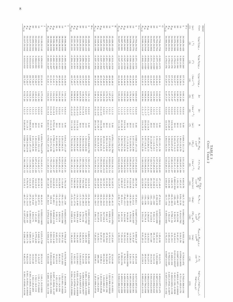
Table 2 presents the derived physical properties for all 10 clouds. The global properties of each cloud were evaluatedfor data extracted out to seven different radii, shown on different lines in the table: 5, 10, 20, and 30 pc using SE;and out to mass weighted (RM ), areal (RA), and half-mass (R1/2) radii using CE. Each cloud definition case is notedin column 1. The center-of-mass coordinates of each cloud are listed in columns 2 and 3, evaluated for the opticallythin and opacity-corrected cases. We note that the CE cloud definitions with RM , RA and R1/2 share the same

7
TABLE
2GMC
PhysicalParametersEst
imates
IRD
C
Case
l CM
,lC
M,τ
bC
M,b
CM,τ
vC
M,v
CM,τ
∆s
∆v
RM
,Mτ
,MG
σ,στ
,σG
dv0
ds
,dv0,τ
ds
θv
,θv,τ
I0,I
0,τ
Erot,0
,Erot,0,τ
β,βτ
log(α
vir
),log(α
vir,τ
),
×104
×10−
2×
103
×1046
(10−
2)
log(α
vir,G
)
(pc)
(
)(
)(km
s−
1)
(pc)
(km
s−
1)
(pc)
(M
)(km
s−
1)
(km
/s/pc)
(deg)
(M
pc2)
(erg)
(1)
(2)
(3)
(4)
(5)
(6)
(7)
(8)
(9)
(10)
(11)
(12)
(13)
(14)
(15)
A 518.8
56,1
8.8
68
-0.2
82,-
0.2
76
64.3
,64.3
2.0
6,2
.12
0.0
,0.0
5.0
01.1
0,1
.87,1
.62
3.9
2,3
.48,1
.66
36.0
,32.3
141,1
24
0.0
814,0
.131
1.3
7,4
.01
7.6
2,3
.39
0.9
12,0
.575,-
0.0
0704
10
18.8
62,1
8.8
75
-0.2
82,-
0.2
82
63.9
,64.1
2.5
8,2
.57
-0.4
,-0.2
10.0
4.8
3,7
.20,5
.73
5.1
2,4
.53,1
.94
15.2
,16.1
124,1
23
1.3
6,1
.97
13.3
,29.6
2.3
4,1
.72
0.8
02,0
.521,-
0.1
15
20
18.8
68,1
8.8
81
-0.3
01,-
0.3
13
63.5
,63.7
3.4
6,4
.02
-0.9
,-0.6
20.0
16.1
,24.0
,19.2
5.8
7,5
.15,2
.36
16.8
,15.6
139,1
42
16.8
,25.7
74.2
,165
6.3
8,3
.78
0.6
96,0
.411,-
0.1
70
30
18.8
68,1
8.8
81
-0.3
07,-
0.3
19
62.6
,63.1
3.7
2,4
.37
-1.7
,-1.3
30.0
31.0
,44.1
,34.9
6.5
8,6
.01,3
.02
12.7
,12.1
96.8
,96.3
68.2
,96.7
183,3
70
5.9
7,3
.80
0.6
88,0
.457,-
0.0
389
RM
18.8
81,1
8.8
93
-0.3
25,-
0.3
37
63.3
,63.5
5.1
0,6
.60
-1.7
,-1.3
17.4
,17.0
9.6
3,1
6.7
,15.7
3.3
8,2
.88,2
.00
17.5
,14.0
151,1
53
7.6
3,1
2.9
30.5
,94.2
7.6
7,2
.69
0.3
80,-
0.0
0984,-
0.2
98
RA
18.8
81,1
8.8
93
-0.3
25,-
0.3
37
63.3
,63.5
5.1
0,6
.60
-1.7
,-1.3
26.6
,26.6
16.6
,28.7
,26.9
3.8
8,3
.36,2
.33
16.5
,14.0
133,1
34
32.3
,54.3
59.3
,177
14.8
,5.9
70.4
47,0
.0862,-
0.2
04
R1/2
18.8
81,1
8.8
93
-0.3
25,-
0.3
37
63.3
,63.5
5.1
0,6
.60
-1.7
,-1.3
17.1
,16.2
9.3
8,1
5.5
,14.7
3.3
4,2
.81,1
.99
17.2
,13.5
151,1
53
7.1
8,1
1.0
29.4
,84.9
7.1
8,2
.36
0.3
74,-
0.0
177,-
0.2
91
B 519.2
99,1
9.2
99
0.0
50,0
.050
27.4
,26.7
1.6
5,1
.46
0.9
,0.6
5.0
00.7
99,1
.38,1
.19
5.2
7,4
.39,1
.59
34.1
,34.3
105,9
7.6
0.0
347,0
.0547
0.7
29,2
.18
5.5
0,2
.94
1.3
1,0
.909,0
.0934
10
19.3
23,1
9.3
30
0.0
32,0
.032
26.9
,26.5
2.9
4,2
.94
0.4
,0.4
10.0
2.3
0,3
.68,2
.88
5.8
8,5
.09,1
.87
67.5
,64.0
114,1
12
0.4
28,0
.603
3.0
1,7
.75
64.3
,31.7
1.2
4,0
.912,0
.150
20
19.3
42,1
9.3
54
0.0
25,0
.025
27.4
,26.9
3.7
2,3
.93
0.9
,0.9
20.0
5.3
5,7
.64,5
.21
6.6
7,6
.18,2
.21
58.2
,57.4
89.3
,89.1
2.7
2,3
.62
8.1
6,1
6.6
112,7
1.2
1.2
9,1
.07,0
.340
30
19.3
17,1
9.3
23
0.0
13,0
.019
27.4
,27.1
3.3
0,3
.10
0.9
,1.1
30.0
7.7
0,1
0.7
,7.2
67.1
4,6
.79,2
.80
42.3
,41.7
87.3
,86.4
6.9
1,9
.34
11.3
,21.9
109,7
3.6
1.3
6,1
.18,0
.577
RM
19.4
47,1
9.4
34
0.0
62,0
.050
24.8
,25.0
7.2
3,6
.78
-1.1
,-0.9
7.7
9,7
.34
1.2
6,2
.35,2
.27
2.2
0,2
.13,1
.78
36.3
,36.5
109,1
12
0.1
95,0
.327
1.1
7,4
.30
21.9
,10.1
0.5
41,0
.219,0
.0764
RA
19.4
47,1
9.4
34
0.0
62,0
.050
24.8
,25.0
7.2
3,6
.78
-1.1
,-0.9
12.2
,12.2
1.8
7,3
.42,3
.26
2.1
9,2
.08,1
.62
31.5
,31.1
100.,101
0.3
53,0
.556
1.6
4,5
.47
21.2
,9.7
70.5
59,0
.256,0
.0577
R1/2
19.4
47,1
9.4
34
0.0
62,0
.050
24.8
,25.0
7.2
3,6
.78
-1.1
,-0.9
7.2
0,6
.60
1.1
2,2
.02,1
.96
2.2
5,2
.19,1
.84
40.8
,41.5
110,1
13
0.1
59,0
.253
0.9
87,3
.54
26.6
,12.2
0.5
81,0
.259,0
.124
C 528.3
70,2
8.3
64
0.0
62,0
.062
78.4
,78.4
0.5
4,0
.76
-0.2
,-0.2
5.0
01.7
5,3
.23,3
.10
4.1
8,3
.49,2
.76
11.6
,11.5
-118,-
114
0.1
10,0
.191
3.5
1,1
1.9
0.4
23,0
.212
0.7
63,0
.341,0
.154
10
28.3
70,2
8.3
64
0.0
55,0
.055
78.6
,78.6
1.0
7,1
.20
0.0
,0.0
10.0
5.7
7,9
.31,8
.82
4.6
7,4
.09,3
.08
6.4
0,6
.77
-74.0
,-86.7
1.3
1,1
.86
19.0
,49.5
0.2
82,0
.171
0.6
43,0
.320,0
.0965
20
28.3
70,2
8.3
58
0.0
49,0
.049
79.0
,79.2
1.6
1,1
.94
0.4
,0.6
20.0
19.7
,28.0
,25.6
5.5
0,5
.16,3
.82
6.6
1,7
.05
-121,-
119
18.7
,25.2
111,2
24
0.7
35,0
.556
0.5
53,0
.344,0
.122
30
28.3
70,2
8.3
64
0.0
31,0
.025
79.0
,79.0
3.2
2,3
.79
0.4
,0.4
30.0
36.7
,50.2
,45.9
5.7
7,5
.50,4
.15
4.5
4,4
.75
-116,-
117
68.0
,88.2
256,4
79
0.5
44,0
.414
0.5
01,0
.324,0
.117
RM
28.3
64,2
8.3
58
0.0
18,0
.012
78.4
,78.4
4.3
3,4
.95
0.2
,0.0
17.1
,16.6
11.4
,17.2
,17.2
3.4
5,3
.27,3
.07
4.5
0,4
.22
-75.6
,-66.2
6.6
0,9
.71
43.5
,102
0.3
06,0
.169
0.3
18,0
.0792,0
.0259
RA
28.3
64,2
8.3
58
0.0
18,0
.012
78.4
,78.4
4.3
3,4
.95
0.2
,0.0
29.0
,29.0
24.4
,36.9
,35.3
4.2
1,4
.21,3
.46
7.7
2,7
.12
-91.4
,-90.5
34.7
,51.6
117,2
68
1.7
5,0
.970
0.3
89,0
.209,0
.0588
R1/2
28.3
64,2
8.3
58
0.0
18,0
.012
78.4
,78.4
4.3
3,4
.95
0.2
,0.0
17.8
,17.2
12.1
,18.2
,18.2
3.4
8,3
.27,3
.09
5.0
9,4
.43
-82.9
,-75.5
7.3
8,1
0.6
47.3
,110
0.4
02,0
.189
0.3
14,0
.0725,0
.0235
D 528.5
73,2
8.5
67
-0.2
33,-
0.2
39
80.7
,82.0
0.6
1,0
.86
0.2
,0.4
5.0
01.9
5,3
.23,2
.09
7.5
9,7
.03,1
.83
20.2
,19.9
-130,-
126
0.1
13,0
.176
4.3
2,1
1.9
1.0
6,0
.583
1.2
4,0
.949,-
0.0
280
10
28.5
79,2
8.5
73
-0.2
33,-
0.2
39
79.6
,80.9
1.2
2,0
.61
-0.9
,-0.6
10.0
5.9
6,9
.23,4
.66
7.6
1,7
.31,1
.88
18.4
,20.1
118,1
12
1.4
2,2
.15
20.3
,48.6
2.3
5,1
.78
1.0
5,0
.828,-
0.0
534
20
28.5
86,2
8.5
92
-0.2
27,-
0.2
33
79.4
,80.3
1.9
3,1
.84
-1.1
,-1.3
20.0
18.5
,27.6
,27.9
7.4
5,7
.47,1
1.7
17.9
,19.3
62.4
,59.4
19.6
,28.8
97.6
,218
6.3
7,4
.92
0.8
45,0
.673,1
.06
30
28.5
73,2
8.5
67
-0.1
96,-
0.2
02
79.6
,80.3
3.7
2,3
.12
-0.9
,-1.3
30.0
36.1
,54.8
,55.1
7.0
7,7
.11,9
.24
8.5
9,1
0.4
50.0
,47.3
81.5
,123
249,5
71
2.4
1,2
.34
0.6
84,0
.509,0
.733
RM
28.5
67,2
8.5
67
-0.1
77,-
0.1
84
79.6
,80.5
5.0
5,4
.45
-1.7
,-1.9
17.6
,18.0
10.5
,18.3
,10.7
6.5
7,6
.74,2
.46
19.9
,23.7
67.6
,63.1
9.3
1,1
6.8
35.8
,106
10.3
,8.8
60.9
26,0
.716,0
.0741
RA
28.5
67,2
8.5
67
-0.1
77,-
0.1
84
79.6
,80.5
5.0
5,4
.45
-1.7
,-1.9
28.2
,28.2
22.1
,37.5
,37.1
6.2
3,6
.53,7
.21
17.4
,20.9
46.3
,44.1
51.4
,87.3
99.1
,285
15.7
,13.3
0.7
61,0
.571,0
.662
R1/2
28.5
67,2
8.5
67
-0.1
77,-
0.1
84
79.6
,80.5
5.0
5,4
.45
-1.7
,-1.9
18.1
,18.5
11.0
,19.2
,11.3
6.5
7,6
.76,2
.51
19.9
,23.9
67.4
,62.3
10.3
,18.9
38.2
,114
10.7
,9.3
50.9
17,0
.709,0
.0795
D-s
528.5
67,2
8.5
67
-0.2
33,-
0.2
39
87.1
,86.9
0.6
1,0
.86
-0.2
,-0.2
5.0
00.9
91,1
.94,1
.96
1.9
7,1
.66,1
.66
4.2
2,5
.23
172,-
177
0.0
874,0
.355
1.1
2,4
.31
0.1
38,0
.224
0.3
58,-
0.0
818,-
0.0
853
10
28.5
73,2
8.5
73
-0.2
39,-
0.2
45
87.5
,87.3
0.6
1,1
.22
0.2
,0.2
10.0
2.4
4,4
.45,4
.41
2.0
6,1
.78,1
.72
11.2
,10.8
124,1
21
0.5
47,0
.968
3.4
1,1
1.3
2.0
2,0
.992
0.3
05,-
0.0
813,-
0.1
09
20
28.6
04,2
8.6
04
-0.2
57,-
0.2
70
88.1
,87.9
3.9
2,4
.78
0.9
,0.9
20.0
6.1
4,1
0.0
,10.2
2.3
9,2
.12,2
.31
14.1
,14.2
64.8
,65.0
5.1
3,7
.54
10.8
,28.7
9.3
9,5
.27
0.3
34,0
.0174,0
.0848
30
28.6
16,2
8.6
10
-0.2
45,-
0.2
57
88.3
,87.9
4.4
6,4
.41
1.1
,0.9
30.0
10.4
,15.9
,16.2
2.5
7,2
.27,2
.52
11.2
,10.5
46.5
,50.2
20.4
,25.8
20.6
,47.9
12.4
,5.9
00.3
45,0
.0551,0
.137
RM
28.6
35,2
8.6
29
-0.2
64,-
0.2
70
87.9
,87.7
6.2
9,6
.12
1.1
,0.9
13.5
,13.4
3.5
8,7
.14,7
.08
1.9
6,1
.90,1
.88
22.3
,22.1
74.4
,78.3
1.2
8,2
.56
5.4
3,2
1.7
11.6
,5.7
20.2
24,-
0.1
02,-
0.1
07
RA
28.6
35,2
8.6
29
-0.2
64,-
0.2
70
87.9
,87.7
6.2
9,6
.12
1.1
,0.9
20.5
,20.5
4.9
1,9
.35,9
.32
2.0
9,2
.03,2
.06
21.5
,20.6
51.6
,60.8
3.1
5,5
.32
6.7
1,2
4.4
21.7
,9.2
00.3
28,0
.0204,0
.0361
R1/2
28.6
35,2
8.6
29
-0.2
64,-
0.2
70
87.9
,87.7
6.2
9,6
.12
1.1
,0.9
11.7
,11.1
3.0
0,5
.76,5
.73
1.8
6,1
.75,1
.72
21.3
,21.4
69.5
,75.4
0.8
90,1
.64
4.4
0,1
7.1
9.1
1,4
.37
0.1
94,-
0.1
64,-
0.1
76
E 528.6
72,2
8.6
84
0.1
30,0
.130
79.4
,79.4
0.5
5,0
.54
-0.4
,-0.6
5.0
00.9
07,1
.27,0
.966
6.6
7,6
.16,2
.71
31.3
,11.8
144,1
28
0.0
571,0
.0742
0.9
39,1
.84
5.9
2,0
.559
1.4
6,1
.24,0
.646
10
28.6
72,2
8.6
90
0.1
18,0
.118
80.7
,81.1
1.2
3,1
.55
0.9
,1.1
10.0
3.5
2,5
.03,4
.20
6.4
5,6
.28,3
.66
18.3
,23.5
74.8
,79.6
0.7
47,1
.01
7.0
8,1
4.5
3.5
2,3
.87
1.1
4,0
.960,0
.568
20
28.6
53,2
8.6
66
0.1
05,0
.099
80.3
,80.5
3.1
0,2
.95
0.4
,0.4
20.0
15.0
,21.1
,18.6
6.5
2,6
.40,4
.32
5.6
9,6
.81
-41.2
,-28.0
15.6
,22.7
63.8
,127
0.7
87,0
.822
0.8
20,0
.655,0
.369
30
28.6
41,2
8.6
47
0.0
81,0
.075
80.3
,80.5
5.4
7,5
.64
0.4
,0.4
30.0
32.4
,46.4
,40.4
6.9
3,6
.87,4
.86
6.3
4,7
.14
-44.8
,-41.1
68.8
,101
199,4
09
1.3
8,1
.25
0.7
14,0
.551,0
.310
RM
28.6
16,2
8.6
22
0.0
56,0
.050
79.8
,80.3
8.2
1,8
.21
0.0
,0.4
17.7
,17.6
9.0
1,1
4.8
,13.7
5.4
7,5
.76,3
.86
14.3
,15.9
-35.2
,-35.6
7.2
9,1
2.1
26.2
,71.3
5.6
6,4
.26
0.8
34,0
.662,0
.349
RA
28.6
16,2
8.6
22
0.0
56,0
.050
79.8
,80.3
8.2
1,8
.21
0.0
,0.4
27.5
,27.5
20.2
,34.2
,31.4
5.4
4,5
.62,4
.02
10.5
,11.3
-8.7
1,-
3.0
140.1
,71.4
84.7
,242
5.1
6,3
.77
0.6
71,0
.472,0
.216
R1/2
28.6
16,2
8.6
22
0.0
56,0
.050
79.8
,80.3
8.2
1,8
.21
0.0
,0.4
18.1
,17.9
9.4
1,1
5.3
,14.1
5.4
7,5
.76,3
.86
14.2
,15.6
-37.2
,-36.3
7.9
3,1
2.8
27.9
,74.2
5.6
7,4
.18
0.8
26,0
.655,0
.344
F 534.4
28,3
4.4
22
0.2
40,0
.240
56.9
,56.9
0.8
9,1
.25
-0.6
,-0.6
5.0
00.8
97,1
.51,1
.30
4.0
9,3
.55,2
.09
20.2
,25.8
75.7
,64.8
0.0
373,0
.0535
0.9
19,2
.60
1.6
5,1
.36
1.0
3,0
.688,0
.289
10
34.4
22,3
4.4
09
0.2
34,0
.228
56.0
,56.3
1.4
3,2
.31
-1.5
,-1.3
10.0
2.8
7,4
.32,3
.68
4.9
9,4
.50,2
.93
25.6
,24.1
109,1
03
0.6
42,0
.861
4.7
0,1
0.7
8.9
2,4
.66
1.0
0,0
.737,0
.434
20
34.4
15,3
4.3
97
0.2
15,0
.209
54.6
,55.0
2.5
4,3
.66
-3.0
,-2.6
20.0
10.6
,16.2
,14.8
5.6
4,5
.25,4
.18
18.0
,18.6
161,1
59
12.6
,19.5
32.0
,74.9
12.8
,8.9
10.8
45,0
.597,0
.438
30
34.4
65,3
4.4
58
0.1
97,0
.197
53.7
,53.9
3.5
5,3
.39
-3.8
,-3.6
30.0
21.3
,31.7
,30.6
6.0
7,5
.79,5
.46
10.3
,11.2
162,1
60
58.7
,88.6
86.1
,191
7.2
1,5
.73
0.7
82,0
.568,0
.531
RM
34.4
71,3
4.4
58
0.2
15,0
.215
53.5
,53.7
2.8
1,2
.32
-3.4
,-3.4
18.9
,18.6
5.0
3,9
.23,7
.44
4.7
6,4
.45,2
.44
25.5
,25.3
-171,-
172
5.8
1,1
0.3
7.6
6,2
6.1
49.1
,25.2
0.9
96,0
.667,0
.240
RA
34.4
71,3
4.4
58
0.2
15,0
.215
53.5
,53.7
2.8
1,2
.32
-3.4
,-3.4
26.2
,26.1
8.9
1,1
6.2
,14.8
4.9
5,4
.84,3
.85
15.7
,16.7
-176,-
178
18.8
,33.9
17.3
,57.5
26.7
,16.4
0.9
23,0
.643,0
.482
R1/2
34.4
71,3
4.4
58
0.2
15,0
.215
53.5
,53.7
2.8
1,2
.32
-3.4
,-3.4
19.6
,19.2
5.3
9,9
.79,7
.91
4.7
9,4
.51,2
.54
24.5
,24.9
-172,-
173
6.6
7,1
1.7
8.4
8,2
8.5
47.2
,25.4
0.9
87,0
.667,0
.261
8
TABLE
3Cont.Table2
IRD
C
Case
lCM
,lCM,τ
bC
M,b
CM,τ
vC
M,v
CM,τ
∆s
∆v
RM
,Mτ
,MG
σ,στ
,σG
dv0
ds
,dv0,τ
ds
θv
,θv,τ
I0,I
0,τ
Erot,0
,Erot,0,τ
β,βτ
log(α
vir
),lo
g(α
vir,τ
),
×104
×10 −
2×
103
×1046
(10 −
2)
log(α
vir,G
)
(pc)
(
)(
)(km
s −1)
(pc)
(km
s −1)
(pc)
(M
)(km
s −1)
(km
/s/pc)
(deg)
(M
pc2)
(erg)
(1)
(2)
(3)
(4)
(5)
(6)
(7)
(8)
(9)
(10)
(11)
(12)
(13)
(14)
(15)
F-s
534.4
28,3
4.4
22
0.2
40,0
.240
57.7
,57.5
0.8
9,1
.25
0.0
,0.0
5.0
00.6
64,1
.21,1
.18
2.5
1,2
.21,1
.77
8.8
5,9
.76
-24.7
,-21.8
0.0
464,0
.0838
0.5
03,1
.68
0.7
18,0
.472
0.7
42,0
.368,0
.192
10
34.4
15,3
4.4
03
0.2
21,0
.221
58.2
,58.0
2.2
5,2
.86
0.4
,0.4
10.0
1.8
9,3
.13,2
.79
2.8
9,2
.67,1
.88
1.8
7,2
.17
9.9
4,-3
.59
0.4
14,0
.783
2.0
4,5
.58
0.0
706,0
.0655
0.7
11,0
.423,0
.170
20
34.3
60,3
4.3
35
0.1
91,0
.184
58.2
,58.0
6.2
8,7
.83
0.4
,0.4
20.0
5.7
4,9
.75,9
.02
2.6
8,2
.48,1
.95
1.0
5,1
.32
-105,-8
8.7
2.4
5,3
.99
9.4
1,2
7.1
0.0
287,0
.0255
0.4
63,0
.167,-0
.00943
30
34.3
79,3
4.3
66
0.1
78,0
.178
58.0
,57.7
5.9
0,6
.47
0.2
,0.2
30.0
9.4
2,1
5.3
,14.3
2.6
1,2
.41,1
.88
0.4
80,0
.504
-129,-1
22
8.3
9,9
.78
16.9
,44.4
0.0
114,0
.00557
0.4
01,0
.122,-0
.0638
RM
34.3
66,3
4.3
54
0.1
78,0
.178
57.3
,57.3
6.4
7,7
.07
0.0
,0.0
14.9
,14.0
3.3
5,6
.67,6
.27
2.2
6,2
.13,1
.67
4.8
6,4
.73
-84.3
,-86.3
0.7
86,1
.34
4.3
1,1
8.1
0.4
28,0
.164
0.4
22,0
.0453,-0
.138
RA
34.3
66,3
4.3
54
0.1
78,0
.178
57.3
,57.3
6.4
7,7
.07
0.0
,0.0
20.5
,20.5
4.0
6,8
.21,7
.84
2.1
4,2
.02,1
.64
4.8
4,4
.96
-80.3
,-77.5
1.5
6,3
.27
4.6
0,1
8.8
0.7
92,0
.425
0.4
31,0
.0733,-0
.0877
R1/2
34.3
66,3
4.3
54
0.1
78,0
.178
57.3
,57.3
6.4
7,7
.07
0.0
,0.0
12.3
,10.9
2.8
4,5
.44,5
.04
2.3
3,2
.20,1
.65
2.6
0,2
.20
-91.7
,-104
0.4
58,0
.602
3.7
3,1
5.5
0.0
827,0
.0187
0.4
37,0
.0511,-0
.162
G534.7
58,3
4.7
58
-0.5
65,-0
.571
43.9
,44.1
0.4
4,0
.88
0.4
,0.9
5.0
01.0
5,1
.61,1
.58
3.5
8,3
.23,2
.85
47.1
,46.0
47.0
,50.8
0.0
575,0
.0804
1.2
5,2
.96
10.2
,5.7
10.8
53,0
.577,0
.475
10
34.7
64,3
4.7
64
-0.5
77,-0
.590
44.6
,44.6
0.9
3,1
.59
1.1
,1.3
10.0
3.1
6,4
.47,4
.14
4.5
7,4
.14,3
.08
12.1
,12.7
-2.5
8,3
.59
0.6
23,0
.698
5.6
9,1
1.4
1.5
9,0
.988
0.8
87,0
.650,0
.425
20
34.8
07,3
4.8
13
-0.6
14,-0
.620
44.8
,44.6
3.5
5,3
.80
1.3
,1.3
20.0
11.1
,14.6
,13.1
6.4
7,6
.29,4
.99
21.8
,22.2
-161,-1
60
9.2
2,1
1.3
35.1
,60.5
12.4
,9.1
40.9
44,0
.802,0
.645
30
34.8
44,3
4.8
62
-0.5
71,-0
.590
44.4
,43.7
4.0
9,4
.92
0.9
,0.4
30.0
21.3
,28.0
,27.7
7.2
2,7
.21,8
.46
20.1
,22.9
-161,-1
58
41.2
,53.6
86.7
,149
19.0
,18.8
0.9
31,0
.812,0
.955
RM
34.9
36,3
4.9
48
-0.6
02,-0
.620
42.0
,41.6
8.9
8,9
.84
-1.5
,-1.7
15.2
,14.8
5.6
5,9
.28,6
.13
5.5
6,5
.91,2
.61
42.4
,56.3
-128,-1
31
3.3
8,6
.07
12.0
,33.3
50.4
,57.5
0.9
84,0
.810,0
.280
RA
34.9
36,3
4.9
48
-0.6
02,-0
.620
42.0
,41.6
8.9
8,9
.84
-1.5
,-1.7
23.9
,23.9
9.0
7,1
4.6
,15.1
5.5
9,5
.66,6
.94
31.7
,35.8
-134,-1
36
9.7
0,1
6.4
19.6
,51.2
49.6
,40.8
0.9
82,0
.784,0
.948
R1/2
34.9
36,3
4.9
48
-0.6
02,-0
.620
42.0
,41.6
8.9
8,9
.84
-1.5
,-1.7
13.9
,13.3
4.9
1,7
.66,5
.30
5.4
8,5
.92,2
.65
42.2
,59.9
-124,-1
28
2.5
3,4
.18
9.9
1,2
5.2
45.3
,59.3
0.9
95,0
.851,0
.313
G-s
534.7
64,3
4.7
64
-0.5
71,-0
.571
44.4
,44.4
0.6
9,0
.69
0.6
,0.9
5.0
00.9
29,1
.47,1
.51
2.5
7,2
.40,2
.66
28.7
,29.1
57.9
,63.1
0.0
487,0
.0714
0.9
85,2
.47
4.0
5,2
.44
0.6
17,0
.357,0
.435
10
34.7
76,3
4.7
70
-0.5
83,-0
.596
44.8
,44.8
1.2
8,1
.87
1.1
,1.3
10.0
2.5
7,3
.81,3
.89
2.7
5,2
.56,2
.77
18.0
,17.8
14.6
,15.2
0.4
08,0
.507
3.7
7,8
.27
3.4
7,1
.94
0.5
34,0
.302,0
.361
20
34.8
38,3
4.8
32
-0.5
90,-0
.602
45.2
,45.2
3.7
6,3
.80
1.5
,1.7
20.0
7.0
1,9
.59,9
.70
2.9
5,2
.81,2
.97
8.1
2,8
.92
-18.9
,-20.1
4.7
9,6
.32
14.0
,26.2
2.2
4,1
.91
0.4
61,0
.282,0
.326
30
34.8
62,3
4.8
62
-0.5
28,-0
.540
45.0
,45.0
4.9
2,4
.76
1.3
,1.5
30.0
11.7
,15.2
,15.4
3.0
3,2
.91,3
.11
1.1
9,1
.35
-26.1
,-23.6
16.8
,20.9
26.0
,44.0
0.0
909,0
.0859
0.4
37,0
.290,0
.339
RM
34.8
87,3
4.8
81
-0.5
47,-0
.559
44.8
,44.8
5.9
5,5
.60
1.1
,1.3
14.5
,14.1
3.6
4,5
.54,5
.58
2.5
8,2
.50,2
.59
13.9
,15.3
-7.8
9,-1
3.1
1.8
4,2
.90
5.2
2,1
2.4
6.7
6,5
.41
0.4
90,0
.266,0
.295
RA
34.8
87,3
4.8
81
-0.5
47,-0
.559
44.8
,44.8
5.9
5,5
.60
1.1
,1.3
21.8
,21.8
5.3
6,7
.95,7
.94
2.5
7,2
.48,2
.50
2.3
8,2
.57
35.9
,14.1
2.4
1,3
.91
7.5
5,1
6.6
0.1
80,0
.154
0.4
93,0
.291,0
.298
R1/2
34.8
87,3
4.8
81
-0.5
47,-0
.559
44.8
,44.8
5.9
5,5
.60
1.1
,1.3
13.1
,12.5
3.2
5,4
.79,4
.87
2.6
2,2
.53,2
.70
16.1
,17.0
-4.8
2,-7
.47
1.4
8,2
.16
4.5
9,1
0.5
8.3
2,5
.91
0.5
08,0
.288,0
.337
H535.4
28,3
5.4
22
-0.3
13,-0
.319
48.6
,48.2
1.1
2,0
.88
1.1
,1.3
5.0
00.9
70,1
.52,0
.789
6.5
3,6
.18,1
.12
51.8
,57.5
-87.4
,-81.5
0.0
500,0
.0761
1.0
7,2
.65
12.4
,9.4
61.4
1,1
.16,-0
.0351
10
35.4
22,3
5.4
22
-0.2
88,-0
.288
48.8
,48.4
1.9
7,2
.27
1.3
,1.5
10.0
3.2
7,5
.02,2
.72
6.8
2,6
.53,1
.54
25.0
,28.7
-68.9
,-68.6
0.6
62,1
.04
6.1
0,1
4.4
6.7
3,5
.91
1.2
2,0
.996,0
.00640
20
35.4
03,3
5.3
97
-0.2
51,-0
.257
49.2
,49.0
3.7
5,3
.79
1.7
,2.1
20.0
9.9
0,1
4.5
,6.6
07.1
6,6
.95,2
.12
31.6
,33.1
-52.4
,-53.3
9.8
0,1
4.7
27.9
,59.6
34.8
,26.8
1.0
8,0
.890,0
.198
30
35.3
67,3
5.3
54
-0.2
82,-0
.307
47.8
,46.9
3.0
8,3
.06
0.2
,0.0
30.0
20.9
,31.0
,31.0
7.9
2,8
.05,1
3.2
32.7
,35.7
-53.9
,-54.6
53.7
,84.0
82.8
,183
69.0
,58.3
1.0
2,0
.863,1
.29
RM
35.3
48,3
5.3
36
-0.3
37,-0
.362
46.5
,45.6
3.4
8,4
.34
-0.2
,-0.6
18.6
,18.6
4.5
2,8
.30,4
.91
5.9
5,5
.90,1
.60
40.4
,40.5
-56.2
,-60.0
4.5
5,8
.61
6.2
7,2
1.1
118,6
6.4
1.2
3,0
.958,0
.0548
RA
35.3
48,3
5.3
36
-0.3
37,-0
.362
46.5
,45.6
3.4
8,4
.34
-0.2
,-0.6
25.7
,25.7
8.2
2,1
5.8
,7.0
77.4
1,7
.53,1
.94
48.5
,49.9
-52.9
,-54.4
18.5
,37.6
15.0
,55.1
288,1
69
1.3
0,1
.03,0
.204
R1/2
35.3
48,3
5.3
36
-0.3
37,-0
.362
46.5
,45.6
3.4
8,4
.34
-0.2
,-0.6
20.0
,19.9
5.0
4,9
.23,5
.14
6.1
9,6
.30,1
.62
43.7
,45.9
-56.1
,-59.7
5.8
9,1
1.1
7.2
5,2
4.4
154,9
5.4
1.2
5,0
.998,0
.0716
H-s
535.4
28,3
5.4
22
-0.3
19,-0
.325
43.9
,43.9
1.5
6,1
.12
0.2
,0.0
5.0
00.4
78,0
.848,0
.781
1.5
0,1
.37,1
.10
13.9
,15.5
-51.8
,-46.3
0.0
321,0
.0616
0.2
60,0
.820
2.3
8,1
.80
0.4
36,0
.108,-0
.0466
10
35.4
16,3
5.4
10
-0.2
94,-0
.301
43.9
,43.9
2.2
7,1
.89
0.2
,0.0
10.0
1.5
0,2
.64,2
.62
1.5
7,1
.47,1
.46
16.2
,16.6
-57.8
,-56.0
0.3
97,0
.740
1.2
9,3
.99
8.0
3,5
.09
0.2
83,-0
.0205,-0
.0250
20
35.3
30,3
5.3
30
-0.2
88,-0
.294
43.7
,43.7
4.4
9,4
.32
0.0
,-0.2
20.0
3.3
6,5
.54,5
.60
1.6
9,1
.60,1
.68
7.8
4,7
.66
-47.5
,-48.3
2.7
9,4
.42
3.2
2,8
.74
5.3
1,2
.95
0.2
98,0
.0293,0
.0677
30
35.2
44,3
5.2
44
-0.2
76,-0
.282
43.7
,43.7
8.6
7,8
.56
0.0
,-0.2
30.0
5.9
9,9
.34,9
.53
1.8
1,1
.72,1
.86
2.8
4,2
.66
-11.7
,-14.5
9.2
9,1
4.4
6.8
2,1
6.6
1.0
9,0
.612
0.2
79,0
.0457,0
.105
RM
35.2
31,3
5.2
31
-0.2
94,-0
.301
43.7
,43.7
8.9
8,8
.61
-0.2
,-0.2
13.4
,13.2
1.8
3,3
.38,3
.47
1.4
0,1
.36,1
.50
5.5
5,4
.94
-14.3
,-9.8
00.9
94,1
.83
1.4
4,4
.93
2.1
2,0
.901
0.2
23,-0
.0746,-0
.00303
RA
35.2
31,3
5.2
31
-0.2
94,-0
.301
43.7
,43.7
8.9
8,8
.61
-0.2
,-0.2
19.2
,19.3
2.9
8,5
.54,5
.60
1.4
8,1
.44,1
.52
3.9
6,3
.86
-8.1
4,-1
7.6
3.2
5,6
.19
2.6
4,9
.06
1.9
2,1
.01
0.2
16,-0
.0739,-0
.0344
R1/2
35.2
31,3
5.2
31
-0.2
94,-0
.301
43.7
,43.7
8.9
8,8
.61
-0.2
,-0.2
13.1
,12.9
1.7
8,3
.23,3
.32
1.4
0,1
.35,1
.49
5.6
1,5
.11
-15.5
,-10.2
0.9
29,1
.64
1.3
8,4
.62
2.1
0,0
.921
0.2
24,-0
.0705,0
.00264
I538.9
36,3
8.9
36
-0.4
60,-0
.460
44.3
,42.6
1.0
4,1
.04
0.6
,0.4
5.0
00.8
14,1
.47,1
.27
5.9
2,4
.47,1
.21
1.7
6,1
4.9
-100.,1
30
0.0
423,0
.0671
0.7
56,2
.47
0.0
172,0
.600
1.4
0,0
.898,-0
.173
10
38.9
30,3
8.9
30
-0.4
54,-0
.460
44.9
,43.2
1.4
5,1
.30
1.3
,1.1
10.0
2.2
5,3
.58,2
.71
6.3
3,5
.26,1
.42
11.9
,6.4
6-3
9.0
,-10.1
0.4
52,0
.588
2.9
0,7
.32
2.2
1,0
.333
1.3
2,0
.955,-0
.0629
20
38.9
42,3
8.9
42
-0.3
93,-0
.411
46.9
,45.4
3.8
1,2
.96
3.2
,3.2
20.0
5.1
5,6
.96,3
.86
6.8
7,6
.42,1
.61
24.3
,22.6
-71.4
,-67.8
2.6
9,3
.54
7.5
7,1
3.8
20.8
,13.1
1.3
3,1
.14,0
.194
30
38.9
61,3
8.9
61
-0.3
62,-0
.380
47.1
,45.6
5.2
2,4
.36
3.4
,3.4
30.0
6.8
1,8
.96,4
.35
7.2
9,6
.94,1
.62
13.5
,15.1
-18.3
,-10.2
9.3
9,1
1.1
8.8
3,1
5.3
19.4
,16.6
1.4
3,1
.27,0
.326
RM
38.9
36,3
8.9
36
-0.4
60,-0
.467
41.3
,41.1
1.0
4,0
.91
0.0
,-0.2
6.7
0,6
.18
0.7
89,1
.61,1
.59
1.4
2,1
.34,1
.27
24.8
,25.9
91.4
,89.1
0.0
849,0
.152
0.5
31,2
.40
9.8
0,4
.24
0.2
97,-0
.0932,-0
.137
RA
38.9
36,3
8.9
36
-0.4
60,-0
.467
41.3
,41.1
1.0
4,0
.91
0.0
,-0.2
11.6
,11.6
1.3
5,2
.71,2
.58
1.7
9,1
.67,1
.32
3.4
3,5
.61
139,1
12
0.2
69,0
.696
0.8
91,3
.61
0.3
53,0
.604
0.5
06,0
.145,-0
.0381
R1/2
38.9
36,3
8.9
36
-0.4
60,-0
.467
41.3
,41.1
1.0
4,0
.91
0.0
,-0.2
6.4
0,5
.70
0.7
55,1
.47,1
.46
1.4
1,1
.29,1
.24
25.1
,25.9
89.1
,84.0
0.0
754,0
.120
0.5
09,2
.17
9.3
3,3
.66
0.2
89,-0
.122,-0
.158
J553.1
39,5
3.1
45
0.0
56,0
.050
21.6
,21.6
0.7
7,0
.98
0.4
,0.4
5.0
00.4
34,0
.794,0
.679
5.4
4,4
.61,1
.11
48.3
,50.5
44.6
,41.5
0.0
222,0
.0403
0.2
15,0
.720
23.9
,14.2
1.6
0,1
.19,0
.0203
10
53.1
64,5
3.1
64
0.0
25,0
.025
22.0
,22.0
1.8
2,1
.82
0.9
,0.9
10.0
0.8
81,1
.53,1
.31
5.1
6,4
.42,1
.17
20.0
,18.1
33.2
,37.5
0.1
32,0
.222
0.4
43,1
.34
11.8
,5.3
71.5
5,1
.17,0
.0849
20
53.2
50,5
3.2
80
0.0
62,0
.050
22.7
,22.7
4.2
5,5
.22
1.5
,1.5
20.0
1.6
5,3
.05,2
.64
4.8
7,4
.17,1
.22
12.2
,10.9
-21.1
,-19.0
1.2
1,2
.26
0.7
75,2
.65
23.2
,10.1
1.5
2,1
.12,0
.119
30
53.2
93,5
3.3
24
0.1
24,0
.105
22.7
,22.7
5.9
9,6
.75
1.5
,1.5
30.0
2.3
1,4
.09,3
.35
5.2
8,4
.59,1
.24
6.8
4,6
.59
10.8
,9.2
32.8
3,4
.71
1.0
1,3
.18
13.0
,6.4
01.6
2,1
.25,0
.203
RM
53.3
17,5
3.3
42
0.0
13,0
.019
22.7
,22.7
6.5
2,7
.24
1.5
,1.5
9.8
9,9
.34
0.6
97,1
.47,1
.50
1.1
0,1
.06,1
.12
12.4
,13.1
-37.2
,-44.5
0.1
89,0
.353
0.2
80,1
.33
10.3
,4.5
40.3
01,-0
.0818,-0
.0402
RA
53.3
17,5
3.3
42
0.0
13,0
.019
22.7
,22.7
6.5
2,7
.24
1.5
,1.5
13.1
,13.1
0.9
39,2
.00,2
.04
1.1
1,1
.08,1
.15
8.7
8,8
.75
-14.4
,-14.9
0.4
83,1
.03
0.3
85,1
.74
9.6
2,4
.53
0.3
01,-0
.0541,-0
.00341
R1/2
53.3
17,5
3.3
42
0.0
13,0
.019
22.7
,22.7
6.5
2,7
.24
1.5
,1.5
9.2
0,8
.60
0.6
29,1
.28,1
.30
1.0
8,1
.06,1
.12
13.3
,15.1
-40.7
,-50.1
0.1
37,0
.227
0.2
46,1
.09
9.8
5,4
.75
0.3
01,-0
.0549,-0
.0138

9
TABLE
4IR
DC
PhysicalParametersEst
imates
IRD
CC
ase
l CM
,lC
M,τ
bC
M,b
CM,τ
vC
M,v
CM,τ
RM
,Mτ
,MG
σ,στ
,σG
dv0
ds
,dv0,τ
ds
θv
,θv,τ
I0,I
0,τ
Erot,0
,Erot,0,τ
β,βτ
log(α
vir
),log(α
vir,τ
),
×104
×10−
2×
103
×1046
(10−
2)
log(α
vir,G
)
(
)(
)(km
s−
1)
(pc)
(M
)(km
s−
1)
(km
/s/pc)
(deg)
(M
pc2)
(erg)
(1)
(2)
(3)
(4)
(5)
(6)
(7)
(8)
(9)
(10)
(11)
(12)
(13)
(14)
ASE
18.8
31,1
8.8
44
-0.2
82,-
0.2
82
64.3
,64.3
5.1
81.0
7,1
.65,1
.41
4.2
0,3
.60,1
.79
24.6
,27.9
117,1
17
143,2
14
123,2
93
6.9
7,5
.66
0.9
98,0
.675,0
.136
CE
18.8
38,1
8.8
44
-0.2
82,-
0.2
76
65.0
,64.8
0.8
02,1
.36,1
.30
2.1
8,1
.97,1
.63
27.1
,28.7
122,1
21
114,1
87
69.4
,199
12.0
,7.7
30.5
53,0
.236,0
.0890
BSE
19.2
68,1
9.2
74
0.0
75,0
.075
26.5
,26.1
1.3
60.0
891,0
.178,0
.170
3.9
6,3
.06,1
.51
37.6
,35.2
-93.6
,-93.5
0.1
02,0
.204
3.2
0,1
2.8
0.4
46,0
.197
1.4
4,0
.920,0
.327
CE
19.2
74,1
9.2
74
0.0
75,0
.075
25.9
,25.9
0.0
742,0
.161,0
.165
1.4
1,1
.33,1
.46
22.8
,22.5
40.5
,40.3
0.7
12,1
.52
2.2
2,1
0.5
1.6
6,0
.727
0.6
25,0
.239,0
.307
CSE
28.3
70,2
8.3
70
0.0
68,0
.068
78.6
,78.6
7.6
83.5
8,6
.19,5
.96
4.0
9,3
.52,2
.83
10.5
,10.6
-98.4
,-102
371,5
99
947,2
830
0.4
29,0
.238
0.6
21,0
.254,0
.0788
CE
28.3
70,2
8.3
70
0.0
68,0
.068
78.1
,78.4
3.0
7,5
.63,5
.68
2.7
8,2
.53,2
.63
14.7
,15.0
-92.7
,-93.8
309,5
27
698,2
340
0.9
56,0
.506
0.3
51,0
.00859,0
.0370
DSE
28.5
67,2
8.5
73
-0.2
33,-
0.2
33
80.5
,81.5
8.4
63.5
4,5
.67,3
.27
7.4
6,7
.09,1
.90
5.6
6,5
.40
-4.1
5,3
7.0
1490,5
28
822,2
110
0.5
77,0
.0727
1.1
9,0
.941,0
.0380
CE
28.5
79,2
8.5
79
-0.2
27,-
0.2
27
81.3
,82.4
2.3
7,4
.29,2
.93
7.0
7,6
.53,1
.71
22.3
,32.3
101,1
07
387,7
27
368,1
210
5.2
1,6
.25
1.3
2,0
.990,-
0.0
0652
D-s
SE
28.5
73,2
8.5
73
-0.2
33,-
0.2
33
87.3
,87.1
8.4
61.6
3,3
.05,3
.05
2.0
6,1
.75,1
.72
6.3
4,7
.73
113,1
14
363,5
84
174,6
12
0.8
34,0
.568
0.4
08,-
0.0
0586,-
0.0
187
CE
28.5
79,2
8.5
79
-0.2
33,-
0.2
33
86.9
,86.9
1.3
5,2
.77,2
.84
1.5
8,1
.49,1
.63
24.3
,24.5
121,1
20
259,4
81
120,5
02
12.7
,5.7
10.2
60,-
0.0
996,-
0.0
343
ESE
28.6
78,2
8.6
78
0.1
30,0
.130
79.8
,80.1
5.7
41.2
9,1
.86,1
.52
6.3
8,5
.97,3
.05
40.7
,41.9
71.4
,69.5
120,1
96
163,3
36
12.2
,10.2
1.3
2,1
.11,0
.611
CE
28.6
72,2
8.6
78
0.1
30,0
.124
79.8
,79.8
0.7
70,1
.26,1
.21
3.5
8,3
.60,2
.41
20.0
,18.5
57.4
,53.4
136,2
51
57.8
,155
9.3
2,5
.53
1.0
5,0
.838,0
.506
FSE
34.4
40,3
4.4
40
0.2
46,0
.246
57.5
,57.5
1.7
50.1
60,0
.294,0
.255
3.7
4,3
.12,1
.67
26.1
,26.9
26.5
,23.8
2.3
8,4
.67
8.2
5,2
8.0
1.9
5,1
.20
1.2
5,0
.831,0
.348
CE
34.4
40,3
4.4
40
0.2
46,0
.246
56.9
,57.1
0.1
22,0
.250,0
.243
1.8
2,1
.69,1
.55
46.8
,46.2
-29.6
,-31.9
2.2
9,4
.58
4.8
2,2
0.3
10.4
,4.7
90.7
42,0
.367,0
.305
F-s
SE
34.4
40,3
4.4
40
0.2
46,0
.246
57.7
,57.5
1.7
50.1
27,0
.252,0
.247
2.1
0,1
.81,1
.58
20.7
,21.1
-23.4
,-23.5
2.6
3,5
.21
5.2
0,2
0.6
2.1
5,1
.12
0.8
51,0
.424,0
.315
CE
34.4
40,3
4.4
40
0.2
46,0
.246
57.3
,57.3
0.1
11,0
.235,0
.239
1.4
4,1
.40,1
.50
32.7
,34.6
-26.5
,-25.9
2.1
8,4
.66
4.0
1,1
7.9
5.8
0,3
.10
0.5
80,0
.230,0
.286
GSE
34.7
64,3
4.7
70
-0.5
59,-
0.5
59
43.5
,43.3
1.5
30.1
39,0
.249,0
.244
3.2
0,2
.75,2
.36
54.8
,49.7
61.4
,60.4
0.8
82,1
.50
7.0
6,2
2.7
3.7
3,1
.62
1.1
2,0
.734,0
.610
CE
34.7
64,3
4.7
64
-0.5
59,-
0.5
59
43.5
,43.3
0.1
27,0
.236,0
.239
2.4
1,2
.17,2
.28
70.5
,67.1
67.0
,66.5
0.6
28,1
.09
5.9
4,2
0.4
5.2
2,2
.40
0.9
12,0
.550,0
.590
G-s
SE
34.7
70,3
4.7
70
-0.5
59,-
0.5
59
43.7
,43.5
1.5
30.1
26,0
.234,0
.236
2.4
2,2
.16,2
.24
33.2
,33.9
72.1
,71.1
0.4
83,0
.861
5.8
7,2
0.0
0.9
02,0
.490
0.9
15,0
.551,0
.579
CE
34.7
70,3
4.7
70
-0.5
59,-
0.5
59
43.7
,43.5
0.1
22,0
.228,0
.233
2.2
3,2
.03,2
.20
36.0
,36.0
69.9
,69.5
0.5
14,0
.902
5.4
2,1
9.1
1.2
2,0
.610
0.8
65,0
.507,0
.569
HSE
35.4
10,3
5.4
10
-0.3
25,-
0.3
31
47.5
,46.9
4.8
40.9
24,1
.56,1
.05
6.1
2,5
.64,1
.42
81.4
,83.0
-60.2
,-60.5
134,2
32
99.3
,282
88.9
,56.3
1.3
6,1
.06,0
.0358
CE
35.4
16,3
5.4
16
-0.3
25,-
0.3
31
46.7
,46.3
0.6
41,1
.24,0
.940
5.0
5,4
.79,1
.24
105,1
06
-61.6
,-61.5
94.5
,187
47.7
,179
218,1
16
1.3
5,1
.02,-
0.0
359
H-s
SE
35.4
03,3
5.4
03
-0.3
37,-
0.3
37
43.7
,43.9
4.8
40.5
60,1
.06,1
.04
1.5
4,1
.43,1
.40
30.6
,29.4
-56.0
,-56.2
95.8
,183
36.5
,130
24.6
,12.2
0.3
80,0
.0397,0
.0277
CE
35.4
03,3
5.3
97
-0.3
37,-
0.3
37
43.9
,43.9
0.4
81,0
.966,0
.940
1.3
4,1
.30,1
.24
41.9
,40.8
-56.2
,-56.2
84.5
,171
26.9
,108
55.0
,26.1
0.3
22,-
0.0
0712,-
0.0
359
ISE
38.9
54,3
8.9
54
-0.4
73,-
0.4
73
43.7
,42.2
1.8
60.1
87,0
.396,0
.361
5.3
3,3
.56,1
.06
17.2
,28.6
150,1
37
3.1
7,5
.27
10.6
,47.7
0.8
71,0
.896
1.5
2,0
.842,-
0.1
69
CE
38.9
54,3
8.9
54
-0.4
73,-
0.4
73
41.3
,41.3
0.1
43,0
.353,0
.356
1.1
0,1
.01,1
.04
27.6
,30.0
-23.1
,-23.3
2.2
0,4
.93
6.2
4,3
8.1
2.6
8,1
.16
0.2
60,-
0.2
06,-
0.1
81
JSE
53.1
14,5
3.1
14
0.0
56,0
.056
21.2
,21.2
0.3
78
0.0
0333,0
.00734,0
.00718
2.3
0,1
.75,0
.728
217,2
08
5.4
5,5
.68
0.0
398,0
.0780
0.0
166,0
.0809
1130,4
16
1.8
4,1
.26,0
.512
CE
53.1
14,5
3.1
14
0.0
56,0
.056
21.2
,21.2
0.0
0298,0
.00693,0
.00707
0.6
98,0
.654,0
.711
1.1
8,7
.40
66.9
,171
0.0
00768,0
.0319
0.0
133,0
.0721
0.0
00795,0
.241
0.8
57,0
.434,0
.497
10
center. Mean velocities are reported in column 4. Columns 5 and 6 list the separations between the GMC centersand the IRDC centers in plane of sky distance and velocity offset, respectively, again for both optically thin andopacity-corrected methods. Column 7 lists the cloud radii (with RM , RA and R1/2 cases having two values for theoptical thin and opacity-corrected cases). Column 8 lists the three cloud mass estimates: optically thin mass (M),opacity-corrected mass (Mτ ), and the mass estimated from a gaussian fit of the co-added opacity corrected columndensity spectra (MG). Column 9 lists the three velocity dispersions measured: the standard deviations of the cloud’soptically thin and opacity corrected column density spectra (σ, στ ) and the dispersion estimated from the gaussianfitted opacity corrected column density spectra (σG). Column 10 presents the two velocity gradient magnitudes, oneestimated from the optically thin column density weighted first-order moment map (dv0/ds) and one estimated fromthe opacity-corrected column density weighted first-order moment map (dv0,τ/ds). Column 11 presents the positionangles of the projected cloud rotation axes estimated from each cloud’s angular momentum for both optically thin andopacity corrected masses (θv and θv,τ ). The projected moments of inertia estimated using the optically thin mass (I0)and opacity corrected mass (I0,τ ) are presented in column 12. Column 13 shows projected rotational energies, Erot,0
and Erot,0,τ , and column 14 shows the ratios of these to the gravitational energy, i.e., β and βτ . Finally, column 15shows log10 of the virial parameters of the clouds using the three measures of mass, i.e., αvir, αvir,τ , αvir,G.
A visual overview of each GMC-scale region is given in Figure 3 and Figures A1-A9. The left side of the figuresdisplay a series of images of the molecular gas out to a radius of 30 pc. The first row displays the GLIMPSE 8µm imageand the 13CO mass surface density map, Σ13CO, generated using the velocity interval given solely by the IRDC. TheIRDC elliptical boundary is also shown (Simon et al. 2006a). The subsequent rows display the Σ13CO maps assumingour defined velocity interval of v0 ± 15 km s−1, the column-density weighted mean velocity (first moment), the linearmomentum map derived from each pixel’s column density and velocity with respect to the cloud center of mass, andthe velocity dispersion map (second moment) for the SE cloud (Left column) and CE cloud (Right column). The rightside of the figures display the optically thin and opacity-corrected co-added column density velocity spectra at variousextraction radii for the SE and CE clouds and the SE IRDC.
Four of the clouds (D, F, G, and H) were found to contain multiple velocity components, based on the co-added13CO column density spectra of their SE 60 pc diameter GMCs (e.g., Cloud D; Fig. A3). We used a series ofintegrated intensity maps to isolate the velocity range of the molecular gas associated with the IRDC (Fig. 4). Ingeneral, these velocity ranges span ∼ 10 km s−1 (Cloud D: 84.1 − 93.7 km s−1; Cloud F: 54.3 − 65.5 km s−1; CloudG: 39.7− 51.8 km s−1; Cloud H: 39.7− 49.9 km s−1). To investigate how the cloud’s derived physical properties wereaffected by isolating only these velocity ranges, we include these four cases as separate entries in Table 2 (noted with“-s”). For all subsequent analyses, the “-s” values for these four clouds are used in place of those derived using thefull velocity range of v0 ± 15 km s−1.
4.2. IRDC and GMC Morphologies
4.2.1. Description of Individual IRDCs/GMCs
Cloud A: We estimate a cloud areal radius of RA ' 27 pc and a mass of MG,A ' 2.7×10⁵ M. The GRS 13CO GMCstudy by RD10 identified five molecular clouds within the extent of Cloud A, with a total 13CO mass of 2.1× 10⁵ M(note, we scaled all 13CO masses of RD10 by a factor 0.49 to convert to our assumed 13CO/H2 abundance ratio; see§3.2). IRDC A is located about 20 pc north of its parent GMC’s highest Σ clump, which appears bright at 8 µm andis thus likely to be star-forming. The WISE H II region catalog (Anderson et al. 2014) lists the W39 H II region tobe within ∼ 3′ of this clump’s center, and with a similar LSR velocity (vLSR = 65.5 km s−1). Another H II region liesin a smaller dense clump at l = 19.07, b = −0.28 with velocity and distance consistent with those of Cloud A. Theisolated, simple 13CO emission profiles, along with the spatial connection between the IRDC and the H II regions,demonstrated through CE, indicates that GMC A contains clumps at a variety of stages of star formation activity.
Cloud B: We estimate a radius of RA ' 12 pc and a mass of MG,A ' 3.3× 10⁴ M. RD10 estimated a 13CO massof 2.4× 10⁴ M and a smaller projected areal radius of 6.3 pc. The IRDC is located within the densest region of theGMC, which extends ∼ 10 pc to the south-east of the IRDC and accounts for most of the cloud’s mass. Spatially,Cloud B is well defined and completely isolated at an extraction radius of 20 pc in CE. Although the cloud is isolatedin velocity space, the column density profile indicates a low level of 13CO emission at neighboring velocities, both lowerand higher. Although the GLIMPSE 8µm emission map indicates a large bright emission structure to the west of thecloud, this feature is not at velocities consistent with Cloud B (vLSR ∼ 50 km s−1).
Cloud C: We estimate a GMC radius of RA ' 29 pc and a mass of MG,A ' 3.5 × 10⁵ M. RD10 derived a radiusof 20.9 pc and a mass of ∼ 3 × 10⁵ M. IRDC C is located within the dense central region of its parent GMC.The integrated intensity maps indicate dense and clumpy structure throughout the cloud (Fig. A2). The velocitydistribution shows a broad centrally-peaked profile, but with potential substructure. Additionally, there is a low levelof 13CO emission at higher velocities. Butler et al. (2014) studied the IRDC C using near- and mid-infrared extinctionmapping to probe the high-dynamic range of its mass surface density (down to AV ∼ 1 mag), finding an IRDC massof ∼ 7 × 10⁴ M. This is one of the most massive, high-Σ IRDCs known, with the potential to form a massive starcluster. Using the same IRDC elliptical boundary from Simon et al. (2006a), we estimate a 13CO mass of 5.7×10⁴M.Our slightly lower mass estimate may be the result of abundance uncertainties and/or CO depletion.
Cloud D: For the GMC at vLSR = 84.1− 93.7 km s−1, we estimate a radius of RA ' 21 pc and a mass of MG,A '9.3 × 10⁴ M. RD10 identified two clouds within the Cloud D-s region with a total 13CO mass of ∼ 5.2 × 10⁴ M.

11
−0.6
−0.4
−0.2
0.0
50
75
100
125
I [M
Jy s
r−1]
−0.6
−0.4
−0.2
0.0
0.000.01
0.02
0.03
0.04
0.050.06
Σ [g c
m−
2]
−0.6
−0.4
−0.2
0.0
−15−10
−5
0
5
1015
v [km
s−
1]
−0.6
−0.4
−0.2
0.0
-150-100
-50
0
50
100150
[MO • km
s-1]
19.2 19.0 18.8 18.6
-0.6
-0.4
-0.2
0.0
19.2 19.0 18.8 18.6
01234567
σ [km
s−
1]
Gala
ctic L
atitu
de
Galactic Longitude
Cloud A
0
2
4
6
8
10SE,5 pcσ=3.48σG=1.66
0
2
4
6
8
10SE,10 pcσ=4.53σG=1.94
0
2
4
6
8
10SE,20 pcσ=5.15σG=2.36
−10 −5 0 5 10 15
0
2
4
6
8
10SE,30 pcσ=6.01σG=3.02
SE,IRDCσ=3.60σG=1.79
CE,RM
σ=2.88σG=2.00
CE,RA
σ=3.36σG=2.33
−10 −5 0 5 10 15
CE,R1/2
σ=2.81σG=1.99
0
2
4
6
8
10
σ=3.92σG=2.25
0
2
4
6
8
10
σ=5.12σG=2.75
0
2
4
6
8
10
σ=5.87σG=3.17
−10 −5 0 5 10 15
0
2
4
6
8
10
σ=6.58σG=4.09
σ=4.20σG=2.33
σ=3.38σG=2.30
σ=3.88σG=2.65
−10 −5 0 5 10 15
σ=3.34σG=2.30
v [vo=64.3,vo,τ=64.5] (km s−1)
N13C
O/d
v (
10
15 c
m−
2 k
m s
−1)
Fig. 3.— Cloud A: Left panel maps: Top row: Left: GLIMPSE 8µm image. Right: 13CO mass surface density (Σ) map over thevelocity range of the IRDC emission profile vlsr = 54.6− 77.1 km s−1 (ellipse denotes IRDC boundary). 2nd row: Left: SE 13CO-derivedΣ map (circles denote 5, 10, 20 pc boundaries). Right: CE 13CO-derived Σ map. 3rd row: Left: SE 13CO mean velocity (first moment)map. Right: CE 13CO mean velocity (first moment) map relative to v0 defined from the IRDC. The arrows show the direction of total(mass-weighted) line-of-sight velocity gradients, dv0/ds. An arrow is shown for each extraction radius (defining the length of the arrow)and is centered on either the extracted cloud’s center of mass (for SE cases) or the R = 30 pc cloud’s center of mass (for CE cases). 4throw: Left: SE 13CO-derived (optically thin) linear momentum map. Right: CE 13CO-derived (optically thin) linear momentum map. Thearrows show the position angle, θv , of the cloud’s rotation axis, i.e., orthogonal to the direction of the velocity gradient, for each extractedcloud (with arrow length showing cloud radius) 5th row: Left: SE 13CO velocity dispersion (second moment; optically thin) map. Right:CE 13CO velocity dispersion (second moment; optically thin) map. All maps in Rows 2-5 cover the velocity interval of v0 ± 15 km s−1,with v0 defined by the emission of the IRDC. Omitted pixels, those that fall below the 5σrms level, are shown in gray. Right panel velocitydistributions: In each panel, the column density distributions with velocity are derived assuming optically thin conditions (blue solid line)or with opacity correction (red solid line) from the 13CO(1-0) co-added spectra. Gaussian fits are shown by the dotted blue and red lines.In all panels, σ and σG are noted in the upper left corner of the plot. Left column: Top to bottom: SE out to R = 5, 10, 20, 30 pc. Rightcolumn: Top to bottom: SE of IRDC ellipse, CE out to RM , RA, R1/2.

12
−0.5
−0.4
−0.3
−0.2
−0.1
0.063.5−70.9
70.9−77.7
28.8 28.7 28.6 28.5 28.4 28.3
−0.5
−0.4
−0.3
−0.2
−0.1
0.077.7−84.1
28.8 28.7 28.6 28.5 28.4 28.3
84.1−93.7
0
10
20
30
40
50
I [K
km
/s]
Ga
lactic L
atitu
de
Galactic Longitude
Cloud D
−0.2
0.0
0.2
0.4
0.6
42.2−47.8
47.8−54.3
34.8 34.6 34.4 34.2 34.0
−0.2
0.0
0.2
0.4
0.6
54.3−65.6
34.8 34.6 34.4 34.2 34.0
65.6−72.4
0
20
40
60
80
I [K
km
/s]
Ga
lactic L
atitu
de
Galactic Longitude
Cloud F
−1.0
−0.8
−0.6
−0.4
−0.2
0.0 28.8−39.7
35.2 35.0 34.8 34.6 34.4 34.2
−1.0
−0.8
−0.6
−0.4
−0.2
0.0 39.7−51.8
35.2 35.0 34.8 34.6 34.4 34.2
51.8−59.0
0
10
20
30
40
50
60
I [K
km
/s]
Ga
lactic L
atitu
de
Galactic Longitude
Cloud G
−0.8
−0.6
−0.4
−0.2
0.0
0.2 32.5−39.7
35.8 35.6 35.4 35.2 35.0
−0.8
−0.6
−0.4
−0.2
0.0
0.2 39.7−49.9
35.8 35.6 35.4 35.2 35.0
49.9−62.6
0
10
20
30
40
50
60
I [K
km
/s]
Ga
lactic L
atitu
de
Galactic Longitude
Cloud H
Fig. 4.— 13CO channel maps of the multi-component clouds. top left : Cloud D; top right : Cloud F; bottom left Cloud G; bottom right :Cloud H. The velocity interval of each panel is shown in the upper-right corner of each map.
The IRDC is located in the dense central region of the GMC. However, the 13CO spectra show four cloud componentswithin v0 ± 15 km s−1. Although the 13CO emission corresponding to the IRDC is evident within a radius of 5 pc,a lower-velocity gas component begins to dominate on scales out to about 20 pc. The position-velocity map (Fig.1) shows there is a significant amount of 13CO emission at lower velocities, vLSR = 63.5-84.1 km s−1, that extendslargely over the northern region of the cloud. In the same velocity interval of the IRDC, vLSR = 84.1− 93.7 km s−1, asubstantial molecular gas clump contains the largest integrated peak intensity (∼ 50 K km s−1) at the western edgeof the 30 pc extraction radius. Figure 4 suggests that this emission is only tenuously connected to the 13CO emissionassociated with the main GMC.
Cloud E: We estimate a GMC radius of RA ' 28 pc and a mass of MG,A ' 3.1 × 10⁵ M. No clouds within theCloud E spatial and velocity ranges were listed in the RD10 catalog. The integrated emission map indicates that theGMC is highly substructured. The IRDC is contained within a small dense clump central to its parent GMC, butmore massive clumps are seen on scales beyond 5 pc. CE finds an extended region of clumpy 13CO gas in the cloud’ssouth-west region, beginning at 10 pc and extending beyond the 30 pc boundary.
Cloud F: For the cloud in the velocity range vLSR = 54.3 − 65.6 km s−1, we estimate a radius of RA ' 21 pc anda mass of MG,A ' 7.8 × 10⁴ M, assuming a distance of 3.7 kpc (Rathborne et al. 2006). Note, Kurayama et al.(2011) estimated a parallax distance 1.56± 0.12 kpc, however this result has been called into question by Foster et al.(2012). RD10 found two GMCs associated with Cloud F: one cloud matches the location and velocity interval of CloudF’s western massive clump, having a mass of ' 6.9 × 10⁴ M and radius of 12.3 pc. The other molecular cloud isassociated with the smaller eastern clump, for which they estimate a mass of ∼ 2.2× 10⁴ M. Our analysis recoversthis larger total mass, ∼ 105M, if we include all the 13CO emission within v0±15 km s−1. The larger molecular cloudcomplex surrounding Cloud F was recently cataloged within the Giant Molecular Filament (GMF) study of Raganet al. (2014). They found that their filament GMF38.1-32.4 is actually the projection of two overlapping filamentarystructures. Cloud F is within the further filament (3.0-3.7 kpc), which has a total length of 232 pc. The GMF containsmultiple infrared dark regions (identified in both GLIMPSE 8µm and HiGAL 250µm images) and several dense gas

13
clumps (identified by the Wienen et al. (2012) NH3 and Bolocam Galactic Plane surveys), demonstrating that overallit is in an early phase of star formation. However, in Cloud F alone, there are two H II regions within the two densestparts of the cloud with consistent LSR velocities and distances, at l = 34.256, b = 0.136 and l = 34.821, b = 0.351(Anderson et al. 2014). While IRDC F, which is also highly filamentary, contains some of the highest column densitiesin the GMC, the highest Σ clump is actually another feature extending west of the IRDC between 5 and 25 pc (Fig.A5). The velocity distribution of the GMC for material out to 30 pc indicates that there are four cloud componentswithin our defined velocity interval v0±15 km s−1. Figure 2 shows the PV maps of the cloud out to 30 pc and indicatesthat the majority of the 13CO emission resides within the velocity interval of the IRDC (vLSR = 54.3− 65.6 km s−1)and is connected to the weaker molecular emission at surrounding velocities. Additionally, the massive clump andIRDC are kinematically associated with another dense clump on the eastern edge of the cloud at ∼ 25 pc. The clouddefined by CE out to a radius of 30 pc indicates that the regions above and below the IRDCs parent cloud are filledwith clumpy molecular material related to the other three emission profiles.
Cloud G: For the material in the velocity range of vlsr = 39.7−51.8 km s−1 we estimate a cloud radius of RA ' 22 pcand a mass of MG,A ' 8.0×10⁴M. RD10 identified two clouds within the Cloud G boundary with a total 13CO massof ∼ 5.7 × 10⁴ M. At small cloud radii, < 10 pc, Cloud G’s velocity distribution is reasonably well described by asingle peak. However, at larger radii we clearly see three separate components within v0± 15 km s−1. The IRDC, andits parent GMC, are confined to the central velocity interval of v = 39.7−51.8 km s−1. In the GMC defined by SE, theIRDC lies at the northern edge of the cloud’s densest region, which extends south ∼ 18 pc. For the cloud defined byCE, this same cloud region breaks up into three smaller clumps. The lower velocity component of the cloud containsa dense molecular clump at l ' 35.2, b ' −0.7, a region which also contains a high level of mid-infrared emission at8µm (Fig. A6). The WISE H II region database lists a candidate H II region near the center of the low-velocity clumpwith an estimated parallax distance of 2.2 kpc, versus the Cloud G distance of 2.9 kpc.
Cloud H: For gas in the velocity range of vlsr = 39.7− 47.1 km s−1, we estimate a cloud radius of RA ' 19 pc and amass of MG,A ' 5.6×10⁴M. RD10 identified three molecular clouds at the location of Cloud H, with a total mass of' 2.8×10⁴M. The PV diagrams indicate that there are three separate cloud components within v0±15 km s−1 (Fig.2). The IRDC and its parent GMC are confined to the velocity interval of v = 39.7− 47.1 km s−1, in which the IRDCis the main structure of a larger diffuse cloud extending to the west. There are additional dense gas clumps at theneighboring velocities: a large coherent clump about 25 pc to the south at v = 32.5− 39.7 km s−1 (part of Cloud G),and a high concentration of dense, clumpy gas along the entire northern region at velocities of v = 47.1− 62.6 km s−1.These higher velocity clumps overlap with a region of bright 8µm dust emission (Fig. A7). The WISE H II databaselists five H II regions overlapping these dense clumps with similar LSR velocities (Anderson et al. 2014).
Cloud I: We find that GMC I has a radius of RA ' 12 pc and a mass of MG,A ' 2.6 × 10⁴ M. However, RD10identified two clouds that match the location of Cloud I, and estimated the much larger mass of ∼ 2.4 × 10⁵ M.This difference is due to the surrounding diffuse 13CO emission, which is included by their cloud finding method thatuses the CLUMPFIND algorithm (Rathborne et al. 2009). IRDC I lies within the densest region of the GMC, whichextends roughly 7 pc north of the IRDC. The cloud’s SE column density spectra indicates a symmetric and wellisolated emission profile out to radii of ∼ 10 pc. However, at larger cloud radii, diffuse 13CO gas at higher velocities isseen. However, the spectra of the cloud defined by CE indicates that this high-velocity emission is at intensities lessthan the 5σ threshold, suggesting that the GMCs is surrounded by a reservoir of low-density molecular gas. For thecloud defined by CE, the central dense region is broken down into three dense clumps and the GLIMPSE 8µm imageindicates that there are multiple bright dust regions along these dense 13CO clumps. However, only one H II regionis identified within the WISE H II catalog, with a slightly lower LSR velocity of ∼ 38 km s−1.
Cloud J: We find that Cloud J has a radius of RA ' 13 pc and a mass of MG,A ' 2.0× 10⁴ M. However, Cloud Jwas included in the GMF catalog by Ragan et al. (2014) in which they estimate a total cloud length of 79 pc. Theyestimated a total cloud mass of 6.8 × 10⁴ M (part of this difference results from the larger considered area; partfrom assuming a smaller n12CO/nH2 ratio of 1.1 × 10⁻⁴). Our analysis also finds that at the largest extraction radii,Cloud J is a filamentary cloud, extending ∼ 60 pc in the CE case. Additionally, the co-added distribution of columndensity with velocity at all cloud radii indicate that Cloud J is quite symmetric and well isolated in velocity space.IRDC J, i.e., G053.11+00.05 from Simon et al. (2006a), defined the search region, but Cloud J also includes the IRDCG053.31+00.00 within its 30 pc radius. The 8µm images of the Cloud J reveal a significant amount of bright dustemission, which Ragan et al. (2014) associated with a foreground high-mass star-forming region at vLSR ∼ 4 km s−1.Our search through the WISE H II database found one radio quiet H II region at l = 53.09, b = 0.12 with an LSRvelocity consistent with Cloud J (Anderson et al. 2014).
4.2.2. Spatial and Velocity Offsets between IRDCs and GMCs
The spatial and velocity offsets between the IRDC and GMC center of masses are listed in Table 2, quoted to thenearest resolution element of the GRS position-velocity grid. In general, spatial offsets grow as one considers largerGMC scales. At the 30 pc aperture scale applied to connected extraction, this offset is typically ∼ 2− 10 pc. All butclouds C and I have this GMC center located outside the Simon et al. (2006a) IRDC boundary.
Velocity offsets are typically relatively small, ∼ 1 km/s. This suggests that IRDCs have been formed by contrac-tion/compression of structures that were already pre-existing within the GMC. Clouds A, B, C, E, I, J have relativelysimple CE CO morphologies in position velocity space. The remaining clouds exhibit more complex, multi-componentstructures.

14
−2
−1
0
−2
−1
0
GMCIRDCABCD −sEF −sG −sH −sIJ
−0.5 0.0 0.5 1.0 1.5
−2
−1
0
−0.5 0.0 0.5 1.0 1.5
log (R/ pc)
log
(dv
0/d
s /
km
s−
1 p
c−
1)
SE,thin CE,thin
SE,τ CE,τ
Fig. 5.— Velocity gradient dv0/ds versus radius R of the clouds over which the gradient is evaluated. Each panel represents a differentcloud definition: (a) Top left: simple extraction, optically thin column density derivation; (b) Bottom left: simple extraction, opacity-corrected column densities; (c) Top right: connected extraction, optically thin column density derivation; (d) Bottom right: connectedextraction, opacity-corrected column densities. n each panel, the 10 IRDCs are shown by the colored filled triangles as defined in the upperright-hand corner. For Clouds D, F, G, and H, these estimates are based on the single component emission profile. GMCs are shownwith filled circles. The best-fit power-law relation from McKee & Ostriker (2007) (dv0/ds ' σpc(s/pc)ασ−1, with values of ασ ' 0.5 andσpc ' 0.72 km s−1) is shown by the dotted lines. The global (IRDCs and GMCs, excluding IRDC J) best-fit power-law relation for eachpanel is shown by the solid lines.
4.3. Kinematics and Dynamics
4.3.1. Velocity Gradients and Implications for Turbulence and Rotation
The GMCs defined by CE have a mean velocity gradient of dv0,τ/ds ' 0.14 km s−1 pc−1. A similar value of0.13 km s−1 pc−1 was found by Imara & Blitz (2011) for five GMCs. The ∼ 100-pc-scale filaments have globalvelocity gradients that are smaller than these values. Jackson et al. (2010) find dv/ds < 0.09 km s−1 pc−1 in “Nessie”,Battersby & Bally (2012) find dv/ds < 0.05 km s−1 pc−1 in their 80-pc long cloud, and Ragan et al. (2014) measuredv/ds ' 0.06 km s−1 pc−1 as an average of the 7 filaments in their sample.
For the elliptical IRDC regions also defined by CE, we find a mean velocity gradient of dv0,τ/ds ' 0.26 km s−1 pc−1,larger than that of the GMCs. For comparison, on smaller scales within IRDC H, Henshaw et al. (2014) find globalvelocity gradients of 0.08, 0.07, 0.30 km s−1 pc−1 in several sub-filaments measured over ∼2 parsec length scales, basedon centroid velocities of the dense gas tracer N2H+(1 − 0). Larger local gradients ∼ 1.5 − 2.5 km s−1 pc−1 can bepresent on sub-parsec scales. Ragan et al. (2012) found velocity gradients of 2.4 and 2.1 kms−1pc−1 within sub-pcregions of IRDCs G5.85-0.23 and G24.05-0.22, based on observations of NH3 (1, 1).
Observed velocity gradients may be a signature of turbulence (e.g., Burkert & Bodenheimer 2000; McKee & Ostriker2007). For a turbulent line-width-size (LWS) relation of the form σ = σpc(s/1 pc)ασ , where values of ασ ' 0.5 andσpc ' 0.72 km s−1 have been reported (McKee & Ostriker 2007), we expect velocity gradients measured over some

15
−0.5
0.0
0.5
1.0
1.5
−0.5
0.0
0.5
1.0
1.5GMCIRDC
ABCD −sEF −sG −sH −sIJ
−0.5
0.0
0.5
1.0
1.5
−0.5 0.0 0.5 1.0 1.5
−0.5
0.0
0.5
1.0
1.5
−0.5 0.0 0.5 1.0 1.5
log (R/ pc)
log(σ
/ k
m s
−1)
SE,thin CE,thin
SE,τ CE,τ
SE,τ,G CE,τ,G
Fig. 6.— Velocity dispersion σ versus radius R of the clouds over which the dispersion is evaluated. Each panel represents a differentcloud definition: (a) Top left: simple extraction, optically thin column density derivation; (b) Middle left: simple extraction, opacity-corrected column densities; (c) Bottom left: simple extraction, opacity-corrected column densities fitted by a Gaussian profile; (d) Topright: connected extraction, optically thin column density derivation; (e) Middle right: connected extraction, opacity-corrected columndensities. (f) Bottom right: connected extraction, opacity-corrected column densities fitted by a Gaussian profile. In each panel, the 10IRDCs are shown by the colored filled triangles as defined in the upper right-hand corner. For Clouds D, F, G, and H, these estimatesare based on the single component emission profile. GMCs are shown with filled circles. The best-fit power-law relation from McKee &Ostriker (2007) (σ = σpc(s/1 pc)ασ , with values of ασ ' 0.5 and σpc ' 0.72 km s−1) is shown by the dotted lines. The global (IRDCs andGMCs) best-fit power-law relation for each panel is shown by the solid lines. In panel (f), the best-fit power-law relations are also shownfor the IRDCs (dot-dashed line) and the GMCs (dashed line).
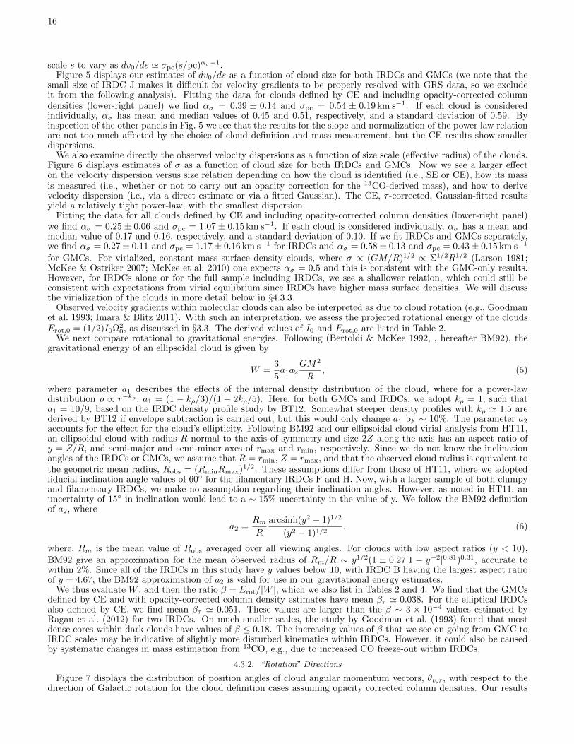
16
scale s to vary as dv0/ds ' σpc(s/pc)ασ−1.Figure 5 displays our estimates of dv0/ds as a function of cloud size for both IRDCs and GMCs (we note that the
small size of IRDC J makes it difficult for velocity gradients to be properly resolved with GRS data, so we excludeit from the following analysis). Fitting the data for clouds defined by CE and including opacity-corrected columndensities (lower-right panel) we find ασ = 0.39 ± 0.14 and σpc = 0.54 ± 0.19 km s−1. If each cloud is consideredindividually, ασ has mean and median values of 0.45 and 0.51, respectively, and a standard deviation of 0.59. Byinspection of the other panels in Fig. 5 we see that the results for the slope and normalization of the power law relationare not too much affected by the choice of cloud definition and mass measurement, but the CE results show smallerdispersions.
We also examine directly the observed velocity dispersions as a function of size scale (effective radius) of the clouds.Figure 6 displays estimates of σ as a function of cloud size for both IRDCs and GMCs. Now we see a larger effecton the velocity dispersion versus size relation depending on how the cloud is identified (i.e., SE or CE), how its massis measured (i.e., whether or not to carry out an opacity correction for the 13CO-derived mass), and how to derivevelocity dispersion (i.e., via a direct estimate or via a fitted Gaussian). The CE, τ -corrected, Gaussian-fitted resultsyield a relatively tight power-law, with the smallest dispersion.
Fitting the data for all clouds defined by CE and including opacity-corrected column densities (lower-right panel)we find ασ = 0.25 ± 0.06 and σpc = 1.07 ± 0.15 km s−1. If each cloud is considered individually, ασ has a mean andmedian value of 0.17 and 0.16, respectively, and a standard deviation of 0.10. If we fit IRDCs and GMCs separately,we find ασ = 0.27± 0.11 and σpc = 1.17± 0.16 km s−1 for IRDCs and ασ = 0.58± 0.13 and σpc = 0.43± 0.15 km s−1
for GMCs. For virialized, constant mass surface density clouds, where σ ∝ (GM/R)1/2 ∝ Σ1/2R1/2 (Larson 1981;McKee & Ostriker 2007; McKee et al. 2010) one expects ασ = 0.5 and this is consistent with the GMC-only results.However, for IRDCs alone or for the full sample including IRDCs, we see a shallower relation, which could still beconsistent with expectations from virial equilibrium since IRDCs have higher mass surface densities. We will discussthe virialization of the clouds in more detail below in §4.3.3.
Observed velocity gradients within molecular clouds can also be interpreted as due to cloud rotation (e.g., Goodmanet al. 1993; Imara & Blitz 2011). With such an interpretation, we assess the projected rotational energy of the cloudsErot,0 = (1/2)I0Ω2
0, as discussed in §3.3. The derived values of I0 and Erot,0 are listed in Table 2.We next compare rotational to gravitational energies. Following (Bertoldi & McKee 1992, , hereafter BM92), the
gravitational energy of an ellipsoidal cloud is given by
W =3
5a1a2
GM2
R, (5)
where parameter a1 describes the effects of the internal density distribution of the cloud, where for a power-lawdistribution ρ ∝ r−kρ , a1 = (1 − kρ/3)/(1 − 2kρ/5). Here, for both GMCs and IRDCs, we adopt kρ = 1, such thata1 = 10/9, based on the IRDC density profile study by BT12. Somewhat steeper density profiles with kρ ' 1.5 arederived by BT12 if envelope subtraction is carried out, but this would only change a1 by ∼ 10%. The parameter a2accounts for the effect for the cloud’s ellipticity. Following BM92 and our ellipsoidal cloud virial analysis from HT11,an ellipsoidal cloud with radius R normal to the axis of symmetry and size 2Z along the axis has an aspect ratio ofy = Z/R, and semi-major and semi-minor axes of rmax and rmin, respectively. Since we do not know the inclinationangles of the IRDCs or GMCs, we assume that R = rmin, Z = rmax, and that the observed cloud radius is equivalent tothe geometric mean radius, Robs = (RminRmax)1/2. These assumptions differ from those of HT11, where we adoptedfiducial inclination angle values of 60 for the filamentary IRDCs F and H. Now, with a larger sample of both clumpyand filamentary IRDCs, we make no assumption regarding their inclination angles. However, as noted in HT11, anuncertainty of 15 in inclination would lead to a ∼ 15% uncertainty in the value of y. We follow the BM92 definitionof a2, where
a2 =RmR
arcsinh(y2 − 1)1/2
(y2 − 1)1/2, (6)
where, Rm is the mean value of Robs averaged over all viewing angles. For clouds with low aspect ratios (y < 10),BM92 give an approximation for the mean observed radius of Rm/R ∼ y1/2(1 ± 0.27|1 − y−2|0.81)0.31, accurate towithin 2%. Since all of the IRDCs in this study have y values below 10, with IRDC B having the largest aspect ratioof y = 4.67, the BM92 approximation of a2 is valid for use in our gravitational energy estimates.
We thus evaluate W , and then the ratio β = Erot/|W |, which we also list in Tables 2 and 4. We find that the GMCsdefined by CE and with opacity-corrected column density estimates have mean βτ ' 0.038. For the elliptical IRDCsalso defined by CE, we find mean βτ ' 0.051. These values are larger than the β ∼ 3 × 10⁻⁴ values estimated byRagan et al. (2012) for two IRDCs. On much smaller scales, the study by Goodman et al. (1993) found that mostdense cores within dark clouds have values of β ≤ 0.18. The increasing values of β that we see on going from GMC toIRDC scales may be indicative of slightly more disturbed kinematics within IRDCs. However, it could also be causedby systematic changes in mass estimation from 13CO, e.g., due to increased CO freeze-out within IRDCs.
4.3.2. “Rotation” Directions
Figure 7 displays the distribution of position angles of cloud angular momentum vectors, θv,τ , with respect to thedirection of Galactic rotation for the cloud definition cases assuming opacity corrected column densities. Our results

17
0.0
0.2
0.4
0.0
0.2
0.4
0.0
0.2
0.4
−180 −90 0 90 180
0.0
0.2
0.4
Retrograde=60.0 %
Retrograde=40.0 %
Retrograde=40.0 %
Retrograde=40.0 %
−90 0 90 180
Retrograde=40.0 %
Retrograde=60.0 %
Retrograde=40.0 %
Retrograde=40.0 %
θv,τ θv,τ
Nc /
NT
S,τ,5 pc
S,τ,10 pc
S,τ,20 pc
S,τ,30 pc
IRDCs: CE,τ
CE,τ,RM
CE,τ,RA
CE,τ,R1/2
Fig. 7.— Distribution of relative position angle of the angular momentum vectors of the 10 IRDCs/GMCs assuming opacity correctedcolumn densities with respect to the direction of Galactic rotation, θv,τ . The effect of different cloud definitions is illustrated in the differentpanels. In each panel, the black line shows the results from the numerical simulation of Tasker & Tan (2009) for clouds at t = 250 Myrand the appropriate inclination of viewing angle of 0 with respect to the galactic plane, i.e., an in-plane view.
show that while a cloud’s position angle can vary depending on cloud definition, the overall, global distribution ofcloud position angles appears consistent with near equal fractions of clouds with prograde and retrograde rotation,although based on a relatively small sample of only 10 analyzed clouds.
Young GMCs, recently formed from the diffuse ISM should possess position angles which are prograde with Galacticrotation (θv < −90; θv > 90). For all of the clouds, measured at various radii for the SE and CE definitions, we findthat there is a large fraction of clouds with retrograde rotation (−90 < θv < +90). We find that ∼ 50% of the CEclouds analyzed with opacity corrected column densities have retrograde motion.
In the Milky Way, Phillips (1999) compiled a database of rotational measurements for 156 individual clouds frompreviously published studies, finding that there is a random distribution between the direction of a cloud’s angularvelocity and the Galactic plane. However, isolated clouds had orientations towards the Galactic poles. They concludedthat the rotation of large-scale structures was due to Galactic shear, while the randomized orientation of cloud positionangles was due to dynamical and/or magnetic interactions. By estimating the velocity gradients for more than 500clouds within the GRS, Koda et al. (2006) found that the populations of prograde and retrograde rotation werenearly equal. Beyond the Milky Way, Rosolowsky et al. (2003) found that 40% of the GMC population in M33 arein retrograde rotation with respect to the galaxy. In a subsequent study of the H I envelopes of 45 GMCs fromRosolowsky et al. (2003), Imara et al. (2011) found that 53% of these GMCs are in retrograde rotation with respectto the local H I. Furthermore, they suggest that if the linear gradients of the H I envelopes are due to rotation, then62% are in retrograde rotation with respect to M33.
In comparison to theoretical models, the disk galaxy simulations of Tasker & Tan (2009) found near equal amountsof apparent prograde and retrograde clouds (∼ 50%) for simulated clouds at t = 250 Myr and a viewing angle of 0
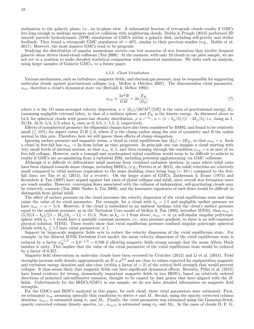
18
inclination to the galactic plane, i.e., an in-plane view. A substantial fraction of retrograde clouds results if GMCslive long enough to undergo mergers and/or collisions with neighboring clouds. Dobbs & Pringle (2013) performed 3Dsmooth particle hydrodynamic (SPH) simulations of GMCs within a galactic disk, including self-gravity and stellarfeedback. They found a retrograde GMC population of ∼ 40%, similar to their previous studies (e.g., Dobbs et al.2011). However, the most massive GMCs tend to be prograde.
Studying the distribution of angular momentum vectors can test scenarios of star formation that involve frequentgalactic shear driven cloud-cloud collisions (Tan 2000). At the moment, with only 10 clouds in our pilot sample, we arenot yet in a position to make detailed statistical comparison with numerical simulations. We defer such an analysis,using larger samples of Galactic GMCs, to a future paper.
4.3.3. Cloud Virialization
Various mechanisms, such as turbulence, magnetic fields, and thermal gas pressure, may be responsible for supportingmolecular clouds against gravitational collapse (e.g., McKee & Ostriker 2007). The dimensionless virial parameter,αvir, describes a cloud’s dynamical state via (Bertoldi & McKee 1992):
αvir ≡5σ2R
GM= 2a
EK|EG|
(7)
where σ is the 1D mass-averaged velocity dispersion, a ≡ |EG|/(3GM2/[5R]) is the ratio of gravitational energy, EG(assuming negligible external tides), to that of a uniform sphere, and EK is the kinetic energy. As discussed above in§4.3, for spherical clouds with power-law density distribution, ρ ∝ r−kρ , a = (1 − kρ/3)/(1 − 2kρ/5), i.e, rising as 1,25/24, 10/9, 5/4, 5/3 when kρ rises as 0, 0.5, 1, 1.5, 2, respectively.
Effects of nonspherical geometry for ellipsoidal clumps have also been considered by BM92, and found to be relativelysmall (. 10%) for aspect ratios Z/R . 6, where Z is the clump radius along the axis of symmetry and R the radiusnormal to this axis. Therefore, here we will ignore these effects of clump elongation.
Ignoring surface pressure and magnetic terms, a cloud in virial equilibrium has |EG| = 2EK , so that αvir = a. Sucha cloud in free-fall has αvir → 2a from below as time progresses. In principle one can imagine a cloud starting withvery small levels of internal motion, so that αvir 1, and then crossing through the condition αvir = a as part of itsfree-fall collapse. However, such a tranquil and synchronized initial condition would seem to be difficult to achieve inreality if GMCs are accumulating from a turbulent ISM, including potential agglomerating via GMC collisions.
Although it is difficult to differentiate infall motions from virialized turbulent motions, in cases where infall rateshave been claimed towards dense clumps, including IRDCs, (e.g., Peretto et al. 2013), the infall velocities are relativelysmall compared to virial motions (equivalent to the mass doubling times being long (∼ 10×) compared to the free-fall time; see Tan et al. (2014), for a review). On the larger scales of GMCs, Zuckerman & Evans (1974) andKrumholz & Tan (2007) have argued against fast rates of global collapse and infall, since overall star formation ratesare much smaller. However, converging flows associated with the collision of independent, self-gravitating clouds maybe relatively common (Tan 2000; Tasker & Tan 2009), and the kinematic signatures of such flows would be difficult todistinguish from global infall.
The effect of surface pressure on the cloud increases the velocity dispersion of the virial equilibrium state and thusraises the value of its virial parameter. For example, for a cloud with kρ = 1.5 and negligible surface pressure wehave αvir = a = 5/4. However, if the cloud is embedded in an ambient medium with the cloud’s surface pressureequal to the ambient pressure, as in the Turbulent Core model of McKee & Tan (2003, hereafter MT03), then αvir =(5/2)(3 − kρ)/[(5 − 2kρ)(kρ − 1)] = 15/4. Note as kρ → 1 from above, αvir → ∞ (a self-similar singular polytropicsphere with kρ = 1 would have a spatially constant pressure, i.e., zero pressure gradient, so there is no self-consistentphysical solution; MT03). These results show that virial equilibrium pressure confined singular polytropic sphericalclouds with kρ . 1.5 have virial parameters 1.
Support by large-scale magnetic fields acts to reduce the velocity dispersion of the virial equilibrium state. Forexample, in the fiducial MT03 Turbulent Core model, the mean velocity dispersion of the virial equilibrium state is
reduced by a factor φ−1/2B → 2.8−1/2 = 0.598 if allowing magnetic fields strong enough that the mean Alfven Mach
number is unity. This implies that the value of the virial parameter of the virial equilibrium state would be reducedby a factor of 0.357.
Magnetic field observations in molecular clouds have been reviewed by Crutcher (2012) and Li et al. (2014). Fieldstrengths increase with density approximately as B ∝ ρ2/3 and are close to values expected for equipartition magneticand turbulent energy densities and also close (within a factor of ∼ 2) of the critical field strength that would preventcollapse. It thus seems likely that magnetic fields can have significant dynamical effects. Recently, Pillai et al. (2015)have found evidence for strong, dynamically important magnetic fields in two IRDCs, based on relatively ordereddirections of polarized sub-millimeter emission, thought to be caused by dust grains that have aligned with the B-fields. Unfortunately for the IRDCs/GMCs in our sample, we do not have detailed information on magnetic fieldstrengths.
For the GMCs and IRDCs analyzed in this paper, for each cloud, three virial parameters were estimated. First,we estimated αvir assuming optically thin conditions to derive σ and M . Second, using the opacity corrected columndensities, αvir,τ is estimated using στ and Mτ . Finally, the virial parameter was estimated using the Gaussian-fitted,opacity corrected column density spectra, i.e., αvir,G is estimated using σG and MG. In the cases of clouds D, F, G,
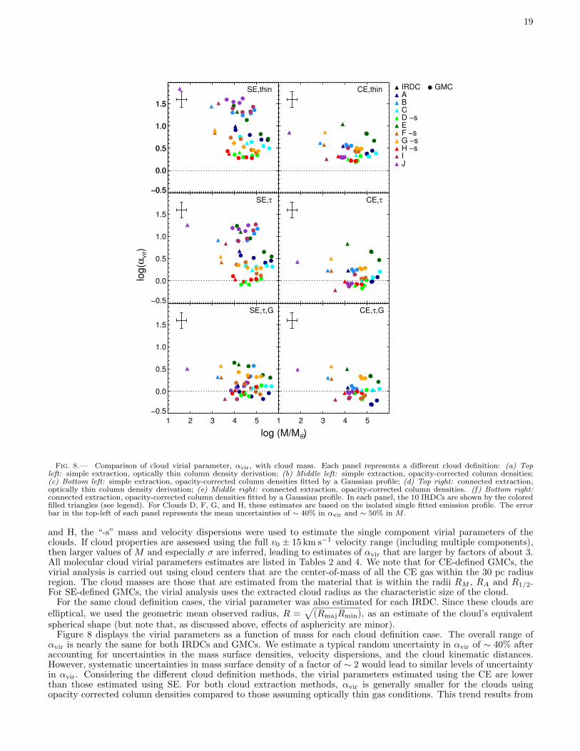
19
−0.5
0.0
0.5
1.0
1.5
−0.5
0.0
0.5
1.0
1.5
GMCIRDCABCD −sEF −sG −sH −sIJ
−0.5
0.0
0.5
1.0
1.5
1 2 3 4 5
−0.5
0.0
0.5
1.0
1.5
1 2 3 4 5
log (M/MO •)
log
(αvir)
SE,thin CE,thin
SE,τ CE,τ
SE,τ,G CE,τ,G
Fig. 8.— Comparison of cloud virial parameter, αvir, with cloud mass. Each panel represents a different cloud definition: (a) Topleft: simple extraction, optically thin column density derivation; (b) Middle left: simple extraction, opacity-corrected column densities;(c) Bottom left: simple extraction, opacity-corrected column densities fitted by a Gaussian profile; (d) Top right: connected extraction,optically thin column density derivation; (e) Middle right: connected extraction, opacity-corrected column densities. (f) Bottom right:connected extraction, opacity-corrected column densities fitted by a Gaussian profile. In each panel, the 10 IRDCs are shown by the coloredfilled triangles (see legend). For Clouds D, F, G, and H, these estimates are based on the isolated single fitted emission profile. The errorbar in the top-left of each panel represents the mean uncertainties of ∼ 40% in αvir and ∼ 50% in M .
and H, the “-s” mass and velocity dispersions were used to estimate the single component virial parameters of theclouds. If cloud properties are assessed using the full v0 ± 15 km s−1 velocity range (including multiple components),then larger values of M and especially σ are inferred, leading to estimates of αvir that are larger by factors of about 3.All molecular cloud virial parameters estimates are listed in Tables 2 and 4. We note that for CE-defined GMCs, thevirial analysis is carried out using cloud centers that are the center-of-mass of all the CE gas within the 30 pc radiusregion. The cloud masses are those that are estimated from the material that is within the radii RM , RA and R1/2.For SE-defined GMCs, the virial analysis uses the extracted cloud radius as the characteristic size of the cloud.
For the same cloud definition cases, the virial parameter was also estimated for each IRDC. Since these clouds areelliptical, we used the geometric mean observed radius, R =
√(RmajRmin), as an estimate of the cloud’s equivalent
spherical shape (but note that, as discussed above, effects of asphericity are minor).Figure 8 displays the virial parameters as a function of mass for each cloud definition case. The overall range of
αvir is nearly the same for both IRDCs and GMCs. We estimate a typical random uncertainty in αvir of ∼ 40% afteraccounting for uncertainties in the mass surface densities, velocity dispersions, and the cloud kinematic distances.However, systematic uncertainties in mass surface density of a factor of ∼ 2 would lead to similar levels of uncertaintyin αvir. Considering the different cloud definition methods, the virial parameters estimated using the CE are lowerthan those estimated using SE. For both cloud extraction methods, αvir is generally smaller for the clouds usingopacity corrected column densities compared to those assuming optically thin gas conditions. This trend results from
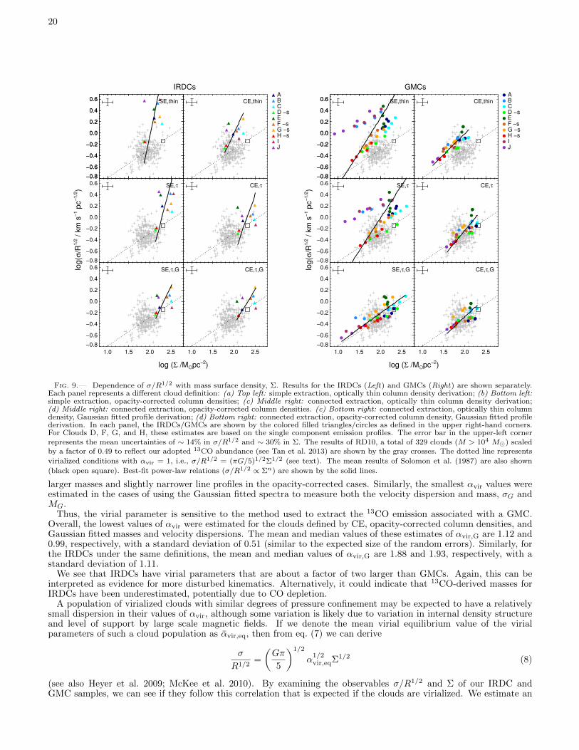
20
−0.8
−0.6
−0.4
−0.2
0.0
0.2
0.4
0.6
−0.8
−0.6
−0.4
−0.2
0.0
0.2
0.4
0.6ABCD −sEF −sG −sH −sIJ
−0.8
−0.6
−0.4
−0.2
0.0
0.2
0.4
0.6
1.0 1.5 2.0 2.5
−0.8
−0.6
−0.4
−0.2
0.0
0.2
0.4
0.6
1.0 1.5 2.0 2.5
log (Σ /MO · pc−2)
log(σ
/R1/2 / k
m s
−1 p
c−
1/2)
IRDCs
SE,thin CE,thin
SE,τ CE,τ
SE,τ,G CE,τ,G
−0.8
−0.6
−0.4
−0.2
0.0
0.2
0.4
0.6
−0.8
−0.6
−0.4
−0.2
0.0
0.2
0.4
0.6ABCD −sEF −sG −sH −sIJ
−0.8
−0.6
−0.4
−0.2
0.0
0.2
0.4
0.6
1.0 1.5 2.0 2.5
−0.8
−0.6
−0.4
−0.2
0.0
0.2
0.4
0.6
1.0 1.5 2.0 2.5
log (Σ /MO · pc−2)
log(σ
/R1/2 / k
m s
−1 p
c−
1/2)
GMCs
SE,thin CE,thin
SE,τ CE,τ
SE,τ,G CE,τ,G
Fig. 9.— Dependence of σ/R1/2 with mass surface density, Σ. Results for the IRDCs (Left) and GMCs (Right) are shown separately.Each panel represents a different cloud definition: (a) Top left: simple extraction, optically thin column density derivation; (b) Bottom left:simple extraction, opacity-corrected column densities; (c) Middle right: connected extraction, optically thin column density derivation;(d) Middle right: connected extraction, opacity-corrected column densities. (c) Bottom right: connected extraction, optically thin columndensity, Gaussian fitted profile derivation; (d) Bottom right: connected extraction, opacity-corrected column density, Gaussian fitted profilederivation. In each panel, the IRDCs/GMCs are shown by the colored filled triangles/circles as defined in the upper right-hand corners.For Clouds D, F, G, and H, these estimates are based on the single component emission profiles. The error bar in the upper-left cornerrepresents the mean uncertainties of ∼ 14% in σ/R1/2 and ∼ 30% in Σ. The results of RD10, a total of 329 clouds (M > 104 M) scaledby a factor of 0.49 to reflect our adopted 13CO abundance (see Tan et al. 2013) are shown by the gray crosses. The dotted line represents
virialized conditions with αvir = 1, i.e., σ/R1/2 = (πG/5)1/2Σ1/2 (see text). The mean results of Solomon et al. (1987) are also shown
(black open square). Best-fit power-law relations (σ/R1/2 ∝ Σn) are shown by the solid lines.
larger masses and slightly narrower line profiles in the opacity-corrected cases. Similarly, the smallest αvir values wereestimated in the cases of using the Gaussian fitted spectra to measure both the velocity dispersion and mass, σG andMG.
Thus, the virial parameter is sensitive to the method used to extract the 13CO emission associated with a GMC.Overall, the lowest values of αvir were estimated for the clouds defined by CE, opacity-corrected column densities, andGaussian fitted masses and velocity dispersions. The mean and median values of these estimates of αvir,G are 1.12 and0.99, respectively, with a standard deviation of 0.51 (similar to the expected size of the random errors). Similarly, forthe IRDCs under the same definitions, the mean and median values of αvir,G are 1.88 and 1.93, respectively, with astandard deviation of 1.11.
We see that IRDCs have virial parameters that are about a factor of two larger than GMCs. Again, this can beinterpreted as evidence for more disturbed kinematics. Alternatively, it could indicate that 13CO-derived masses forIRDCs have been underestimated, potentially due to CO depletion.
A population of virialized clouds with similar degrees of pressure confinement may be expected to have a relativelysmall dispersion in their values of αvir, although some variation is likely due to variation in internal density structureand level of support by large scale magnetic fields. If we denote the mean virial equilibrium value of the virialparameters of such a cloud population as αvir,eq, then from eq. (7) we can derive
σ
R1/2=
(Gπ
5
)1/2
α1/2vir,eqΣ1/2 (8)
(see also Heyer et al. 2009; McKee et al. 2010). By examining the observables σ/R1/2 and Σ of our IRDC andGMC samples, we can see if they follow this correlation that is expected if the clouds are virialized. We estimate an

21
1.4 1.6 1.8 2.0 2.2 2.4 2.6
−0.6
−0.4
−0.2
0.0
0.2
0.4
α vir=0.5
α vir=1
α vir=2
α vir=4
α vir=8
log (Σ /MO · pc−2)
log(σ
/R1
/2 / k
m s
−1 p
c−
1/2)
CE,τ,GGMCIRDC
ABCD −sEF −sG −sH −sIJ
Fig. 10.— Dependence of σ/R1/2 with mass surface density, Σ, for the all clouds defined by CE, opacity corrected column densities,and gaussian fitted velocity dispersions. As in Figure 9, IRDCs are shown by the filled triangles and the GMCs by the filled circles (see
legend). The error bar in the upper-left corner represents the mean uncertainties of ∼ 14% in σ/R1/2 and ∼ 30% in Σ. The results ofRD10, a total of 329 clouds with M > 104 M, are shown by the gray crosses. The mean results of Solomon et al. (1987) are also shown
(open black square). The best-fit power-law relation (σ/R1/2 ∝ Σn) is shown for both the IRDCs (n = 1.27± 0.52; dot-dashed line) andthe GMCs (n = 0.70 ± 0.12; dashed line). Collectively, the IRDCs and GMCs have a best-fit power-law relation of n = 0.81± 0.10 (solidline). The dotted lines represents the expected scaling relation for virialized clouds with different values of αvir = 0.5, 1, 2, 4, and 8.
uncertainty in σ/R1/2 of ∼ 14% based on 10% uncertainties in both σ and R.Thus we considered the above scaling relationship for the results of our ten IRDCs and GMCs (Fig. 9). For IRDCs,
Σ was estimated for each ellipsoidal cloud using the geometric mean observed radius R and the total 13CO-derivedmass. For GMCs, Σ was estimated using the circular area defined by the extraction radius R and its corresponding13CO-derived mass. We estimate a random uncertainty in Σ of ∼ 30% based on the uncertainty in Tex and potentialvariations in our assumed abundances. However, systematic uncertainties could be present at the factor of ∼ 2 level.
For the ten GMCs, we find that the clouds analyzed using gaussian profile fitting on the opacity corrected columndensity spectra to estimate the cloud mass and velocity dispersion, yield results most consistent with the scalingexpected for gravitational virial equilibrium. Specifically, we find the best-fit power-law relation σ/R1/2 ∝ Σn hasn = 0.54 ± 0.05 and n = 0.70 ± 0.12, for the SE and CE extraction, respectively. We gauge the significance of thesefits by estimating the Pearson’s correlation coefficient, ρ, and the one-sided p-value. For all the GMCs defined by CEand gaussian profile fitting on the opacity corrected column density spectra, we estimate ρ = 0.71 and a p-value of6.0× 10−6, indicating a significant linearity in the data.
On the other hand, for the ten IRDCs analyzed using gaussian profile fitting on the opacity corrected columndensity spectra to estimate the cloud mass and velocity dispersion, yield steeper best-fit power-law relations, withn = 1.57 ± 0.80 and n = 1.27 ± 0.52, for the SE and CE extraction, respectively. These power-law fits are lesssignificant than those seen for the GMCs, with ρ = 0.56 and a p-value of 0.047 for the “CE,τ ,G” method.
Focusing on the “CE,τ ,G” extraction method, these IRDC and GMC results are displayed together in Fig. 10.Overall the IRDCs and GMCs together yield a best-fit power-law relation of n = 0.81± 0.10, somewhat steeper thanthe n = 1/2 expected for virialized clouds. If a power-law relation with n = 0.5 is fit, then the normalization impliesαvir = 1.60 and 1.03 for IRDCs and GMCs, respectively, and αvir = 1.15 for the whole sample (with a Pearson’scorrelation coefficient of ρ = 0.78 with a p-value of 1.7 × 10⁻⁹). We note that some of the dispersion in the data isdue to cloud-to-cloud variation, which might be expected if there is systematic variation in degree of surface pressureconfinement, magnetization, distance uncertainty (affecting R) or 13CO abundance.
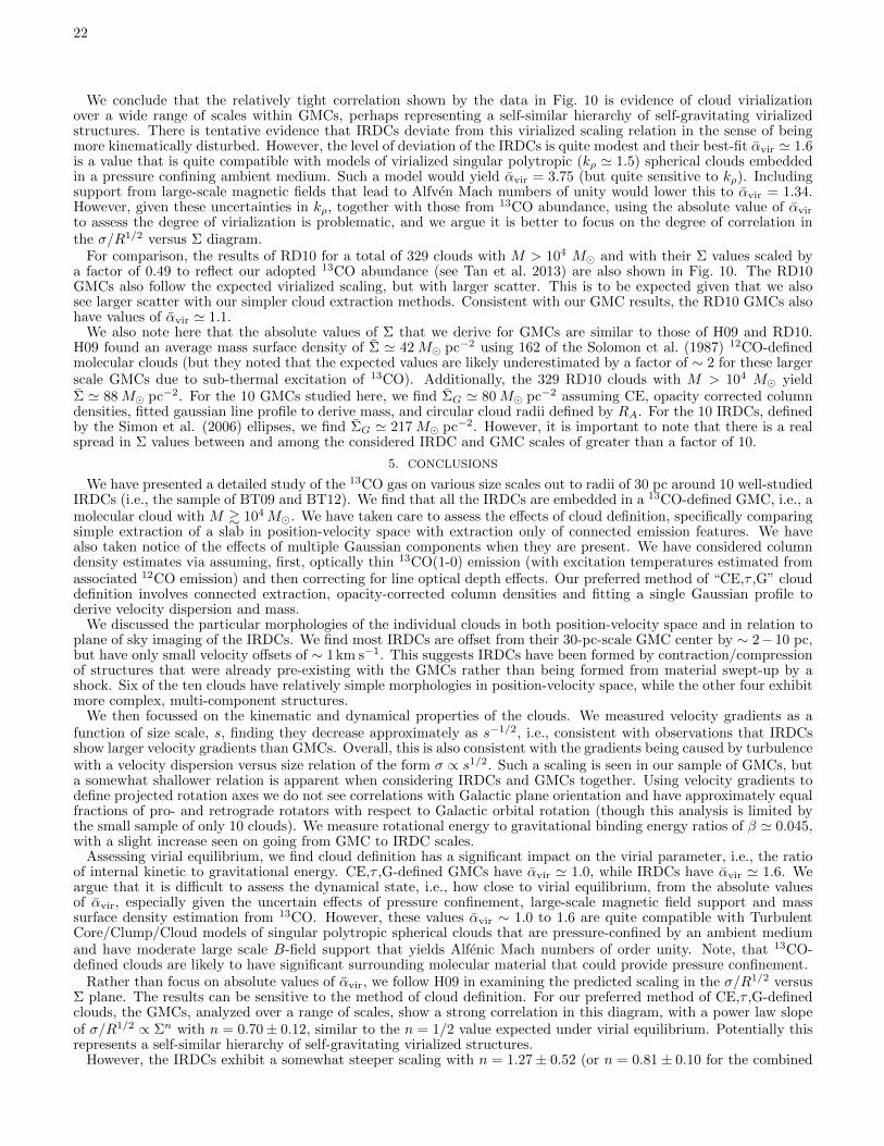
22
We conclude that the relatively tight correlation shown by the data in Fig. 10 is evidence of cloud virializationover a wide range of scales within GMCs, perhaps representing a self-similar hierarchy of self-gravitating virializedstructures. There is tentative evidence that IRDCs deviate from this virialized scaling relation in the sense of beingmore kinematically disturbed. However, the level of deviation of the IRDCs is quite modest and their best-fit αvir ' 1.6is a value that is quite compatible with models of virialized singular polytropic (kρ ' 1.5) spherical clouds embeddedin a pressure confining ambient medium. Such a model would yield αvir = 3.75 (but quite sensitive to kρ). Includingsupport from large-scale magnetic fields that lead to Alfven Mach numbers of unity would lower this to αvir = 1.34.However, given these uncertainties in kρ, together with those from 13CO abundance, using the absolute value of αvir
to assess the degree of virialization is problematic, and we argue it is better to focus on the degree of correlation inthe σ/R1/2 versus Σ diagram.
For comparison, the results of RD10 for a total of 329 clouds with M > 104 M and with their Σ values scaled bya factor of 0.49 to reflect our adopted 13CO abundance (see Tan et al. 2013) are also shown in Fig. 10. The RD10GMCs also follow the expected virialized scaling, but with larger scatter. This is to be expected given that we alsosee larger scatter with our simpler cloud extraction methods. Consistent with our GMC results, the RD10 GMCs alsohave values of αvir ' 1.1.
We also note here that the absolute values of Σ that we derive for GMCs are similar to those of H09 and RD10.H09 found an average mass surface density of Σ ' 42 M pc−2 using 162 of the Solomon et al. (1987) 12CO-definedmolecular clouds (but they noted that the expected values are likely underestimated by a factor of ∼ 2 for these largerscale GMCs due to sub-thermal excitation of 13CO). Additionally, the 329 RD10 clouds with M > 104 M yieldΣ ' 88M pc−2. For the 10 GMCs studied here, we find ΣG ' 80M pc−2 assuming CE, opacity corrected columndensities, fitted gaussian line profile to derive mass, and circular cloud radii defined by RA. For the 10 IRDCs, definedby the Simon et al. (2006) ellipses, we find ΣG ' 217M pc−2. However, it is important to note that there is a realspread in Σ values between and among the considered IRDC and GMC scales of greater than a factor of 10.
5. CONCLUSIONS
We have presented a detailed study of the 13CO gas on various size scales out to radii of 30 pc around 10 well-studiedIRDCs (i.e., the sample of BT09 and BT12). We find that all the IRDCs are embedded in a 13CO-defined GMC, i.e., amolecular cloud with M & 104M. We have taken care to assess the effects of cloud definition, specifically comparingsimple extraction of a slab in position-velocity space with extraction only of connected emission features. We havealso taken notice of the effects of multiple Gaussian components when they are present. We have considered columndensity estimates via assuming, first, optically thin 13CO(1-0) emission (with excitation temperatures estimated fromassociated 12CO emission) and then correcting for line optical depth effects. Our preferred method of “CE,τ ,G” clouddefinition involves connected extraction, opacity-corrected column densities and fitting a single Gaussian profile toderive velocity dispersion and mass.
We discussed the particular morphologies of the individual clouds in both position-velocity space and in relation toplane of sky imaging of the IRDCs. We find most IRDCs are offset from their 30-pc-scale GMC center by ∼ 2− 10 pc,but have only small velocity offsets of ∼ 1km s−1. This suggests IRDCs have been formed by contraction/compressionof structures that were already pre-existing with the GMCs rather than being formed from material swept-up by ashock. Six of the ten clouds have relatively simple morphologies in position-velocity space, while the other four exhibitmore complex, multi-component structures.
We then focussed on the kinematic and dynamical properties of the clouds. We measured velocity gradients as afunction of size scale, s, finding they decrease approximately as s−1/2, i.e., consistent with observations that IRDCsshow larger velocity gradients than GMCs. Overall, this is also consistent with the gradients being caused by turbulencewith a velocity dispersion versus size relation of the form σ ∝ s1/2. Such a scaling is seen in our sample of GMCs, buta somewhat shallower relation is apparent when considering IRDCs and GMCs together. Using velocity gradients todefine projected rotation axes we do not see correlations with Galactic plane orientation and have approximately equalfractions of pro- and retrograde rotators with respect to Galactic orbital rotation (though this analysis is limited bythe small sample of only 10 clouds). We measure rotational energy to gravitational binding energy ratios of β ' 0.045,with a slight increase seen on going from GMC to IRDC scales.
Assessing virial equilibrium, we find cloud definition has a significant impact on the virial parameter, i.e., the ratioof internal kinetic to gravitational energy. CE,τ ,G-defined GMCs have αvir ' 1.0, while IRDCs have αvir ' 1.6. Weargue that it is difficult to assess the dynamical state, i.e., how close to virial equilibrium, from the absolute valuesof αvir, especially given the uncertain effects of pressure confinement, large-scale magnetic field support and masssurface density estimation from 13CO. However, these values αvir ∼ 1.0 to 1.6 are quite compatible with TurbulentCore/Clump/Cloud models of singular polytropic spherical clouds that are pressure-confined by an ambient mediumand have moderate large scale B-field support that yields Alfenic Mach numbers of order unity. Note, that 13CO-defined clouds are likely to have significant surrounding molecular material that could provide pressure confinement.
Rather than focus on absolute values of αvir, we follow H09 in examining the predicted scaling in the σ/R1/2 versusΣ plane. The results can be sensitive to the method of cloud definition. For our preferred method of CE,τ ,G-definedclouds, the GMCs, analyzed over a range of scales, show a strong correlation in this diagram, with a power law slopeof σ/R1/2 ∝ Σn with n = 0.70± 0.12, similar to the n = 1/2 value expected under virial equilibrium. Potentially thisrepresents a self-similar hierarchy of self-gravitating virialized structures.
However, the IRDCs exhibit a somewhat steeper scaling with n = 1.27± 0.52 (or n = 0.81± 0.10 for the combined
23
GMC and IRDC sample). This may indicate that IRDCs have moderately more disturbed kinematics than GMCs,which is qualitative expectation of models in which star formation is triggered by GMC-GMC collisions (e.g., Scovilleet al. 1986; Tan 2000). However, it is also possible that systematic uncertainties affecting mass surface densityestimation from 13CO, such as increased CO freeze-out in IRDCs (e.g., Hernandez et al. 2011, 2012), are playing arole. Improved methods of measuring mass and assessing degree of CO freeze-out in these clouds are needed to helpdistinguish these possibilities and thus reliably measure the dynamical state of gas that is likely to form star clusters.
Additional future work will involve applying the techniques developed here to larger samples of clouds to betterstudy connections with Galactic dynamics and Galactic environment, and potential systematic differences of GMCsthat are forming IRDCs or that have relatively high dense gas mass fractions.
A.K.H acknowledges support from grants awarded to Bart Wakker at the University of Wisconsin-Madison. Wethank Brian Babler for contributing to the GLIMPSE data processing. This publication makes use of molecularline data from the Boston University-FCRAO Galactic Ring Survey (GRS). The GRS is a joint project of BostonUniversity and Five College Radio Astronomy Observatory, funded by the National Science Foundation under grantsAST-9800334, AST-0098562, and AST-0100793. J.C.T. acknowledges support from NASA grants ATP09-0094 andADAP10-0110.

24
APPENDIX
A. CLOUD MAPS: B-J
−0.6
−0.4
−0.2
0.0
0.2
0.4
0.6
60
80
100
120
140
I [M
Jy s
r−1]
−0.6
−0.4
−0.2
0.0
0.2
0.4
0.6
0.00
0.01
0.02
0.03
Σ [
g c
m−
2]
−0.6
−0.4
−0.2
0.0
0.2
0.4
0.6
−15−10
−5
0
5
1015
v [
km
s−
1]
−0.6
−0.4
−0.2
0.0
0.2
0.4
0.6
-50
-25
0
25
50
[MO •
km
s-1]
19.6 19.2 18.8
-0.6
-0.4
-0.2
0.0
0.2
0.4
0.6
19.6 19.2 18.8
0
1
2
3
4
5
σ [
km
s−
1]
Gala
ctic L
atitu
de
Galactic Longitude
Cloud B
0
2
4
6
8
10
12
14SE,5 pcσ=4.39σG=1.66
0
2
4
6
8
10
12
14SE,10 pcσ=5.09σG=1.94
0
2
4
6
8
10
12
14SE,20 pcσ=6.18σG=2.36
−10 −5 0 5 10 15
0
2
4
6
8
10
12
14SE,30 pcσ=6.79σG=3.02
SE,IRDCσ=3.06σG=1.51
CE,RM
σ=2.13σG=2.00
CE,RA
σ=2.08σG=2.33
−10 −5 0 5 10 15
CE,R1/2
σ=2.19σG=1.99
0
2
4
6
8
10
12
14
σ=5.27σG=2.25
0
2
4
6
8
10
12
14
σ=5.88σG=2.75
0
2
4
6
8
10
12
14
σ=6.67σG=3.17
−10 −5 0 5 10 15
0
2
4
6
8
10
12
14
σ=7.14σG=4.09
σ=3.96σG=1.68
σ=2.20σG=2.30
σ=2.19σG=2.65
−10 −5 0 5 10 15
σ=2.25σG=2.30
v [vo=26.5,vo,τ=26.7] (km s−1)
N1
3C
O/d
v (
10
15 c
m−
2 k
m s
−1)
Fig. A1.— Same as Fig. 3, but for Cloud B. The 13CO(1-0) GRS integrated intensity map of the IRDC emission profile is over thevelocity range: vLSR = 20.7− 31.6 km s−1.

25
−0.2
−0.1
0.0
0.1
0.2
0.3
45
60
75
90
105
120
I [M
Jy s
r−1]
−0.2
−0.1
0.0
0.1
0.2
0.3
0.00
0.01
0.02
0.03
0.04
0.05
Σ [
g c
m−
2]
−0.2
−0.1
0.0
0.1
0.2
0.3
−12−9−6−3036912
v [
km
s−
1]
−0.2
−0.1
0.0
0.1
0.2
0.3
-150-100
-50
0
50
100150
[MO •
km
s-1]
28.6 28.4 28.2
-0.2
-0.1
0.0
0.1
0.2
0.3
28.6 28.4 28.2
012345678
σ [
km
s−
1]
Gala
ctic L
atitu
de
Galactic Longitude
Cloud C
0
2
4
6
8
10
12SE,5 pcσ=3.49σG=1.66
0
2
4
6
8
10
12SE,10 pcσ=4.09σG=1.94
0
2
4
6
8
10
12SE,20 pcσ=5.16σG=2.36
−10 −5 0 5 10 15
0
2
4
6
8
10
12SE,30 pcσ=5.50σG=3.02
SE,IRDCσ=3.52σG=2.83
CE,RM
σ=3.27σG=2.00
CE,RA
σ=4.21σG=2.33
−10 −5 0 5 10 15
CE,R1/2
σ=3.27σG=1.99
0
2
4
6
8
10
12
σ=4.18σG=2.25
0
2
4
6
8
10
12
σ=4.67σG=2.75
0
2
4
6
8
10
12
σ=5.50σG=3.17
−10 −5 0 5 10 15
0
2
4
6
8
10
12
σ=5.77σG=4.09
σ=4.09σG=3.51
σ=3.45σG=2.30
σ=4.21σG=2.65
−10 −5 0 5 10 15
σ=3.48σG=2.30
v [vo=79.0,vo,τ=79.2] (km s−1)
N1
3C
O/d
v (
10
15 c
m−
2 k
m s
−1)
Fig. A2.— Same as Fig. 3, but for Cloud C. The 13CO(1-0) GRS integrated intensity map of the IRDC emission profile is over thevelocity range: vLSR = 66.3− 85.7 km s−1.
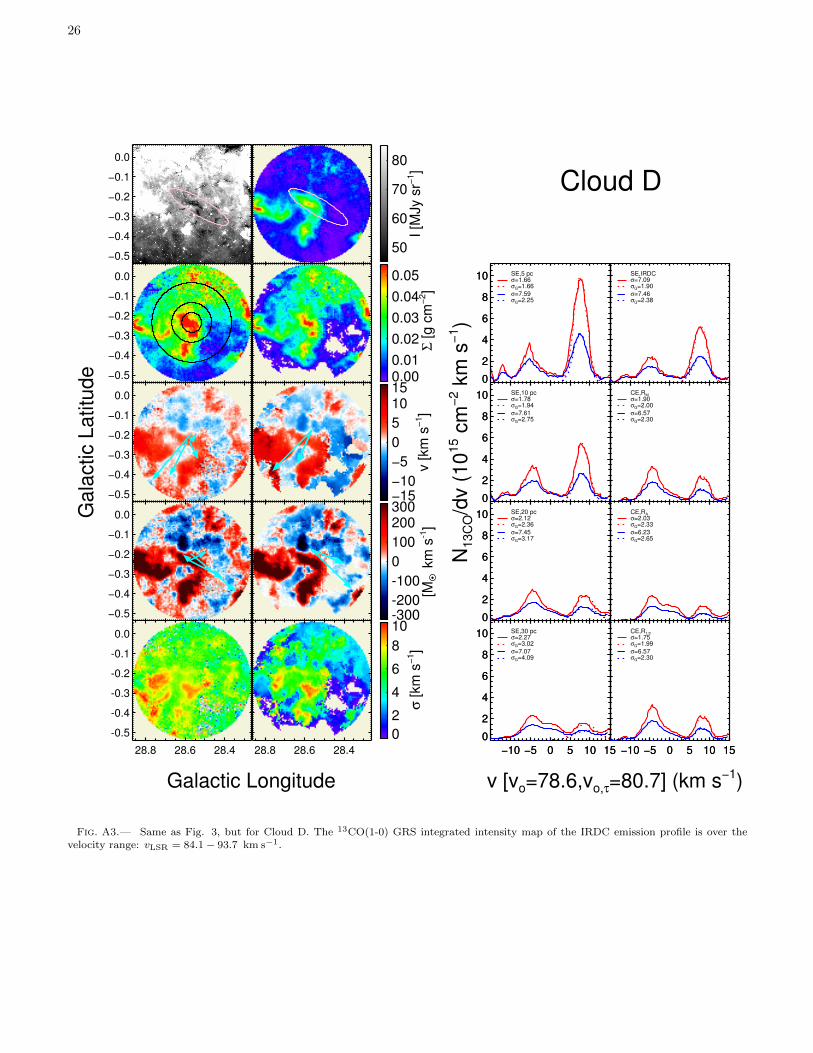
26
−0.5
−0.4
−0.3
−0.2
−0.1
0.0
50
60
70
80
I [M
Jy s
r−1]
−0.5
−0.4
−0.3
−0.2
−0.1
0.0
0.000.01
0.02
0.03
0.04
0.05
Σ [
g c
m−
2]
−0.5
−0.4
−0.3
−0.2
−0.1
0.0
−15−10
−5
0
5
1015
v [
km
s−
1]
−0.5
−0.4
−0.3
−0.2
−0.1
0.0
-300-200
-100
0
100
200300
[MO •
km
s-1]
28.8 28.6 28.4
-0.5
-0.4
-0.3
-0.2
-0.1
0.0
28.8 28.6 28.4
0
2
4
6
8
10
σ [
km
s−
1]
Gala
ctic L
atitu
de
Galactic Longitude
Cloud D
0
2
4
6
8
10 SE,5 pcσ=1.66σG=1.66
0
2
4
6
8
10 SE,10 pcσ=1.78σG=1.94
0
2
4
6
8
10 SE,20 pcσ=2.12σG=2.36
−10 −5 0 5 10 15
0
2
4
6
8
10 SE,30 pcσ=2.27σG=3.02
SE,IRDCσ=7.09σG=1.90
CE,RM
σ=1.90σG=2.00
CE,RA
σ=2.03σG=2.33
−10 −5 0 5 10 15
CE,R1/2
σ=1.75σG=1.99
0
2
4
6
8
10
σ=7.59σG=2.25
0
2
4
6
8
10
σ=7.61σG=2.75
0
2
4
6
8
10
σ=7.45σG=3.17
−10 −5 0 5 10 15
0
2
4
6
8
10
σ=7.07σG=4.09
σ=7.46σG=2.38
σ=6.57σG=2.30
σ=6.23σG=2.65
−10 −5 0 5 10 15
σ=6.57σG=2.30
v [vo=78.6,vo,τ=80.7] (km s−1)
N1
3C
O/d
v (
10
15 c
m−
2 k
m s
−1)
Fig. A3.— Same as Fig. 3, but for Cloud D. The 13CO(1-0) GRS integrated intensity map of the IRDC emission profile is over thevelocity range: vLSR = 84.1− 93.7 km s−1.
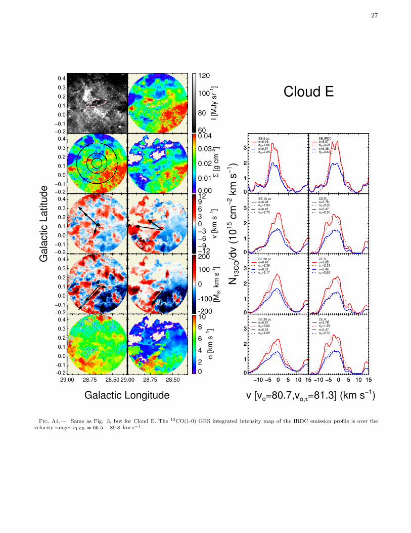
27
−0.2
−0.1
0.0
0.1
0.2
0.3
0.4
60
80
100
120
I [M
Jy s
r−1]
−0.2
−0.1
0.0
0.1
0.2
0.3
0.4
0.00
0.01
0.02
0.03
0.04
Σ [
g c
m−
2]
−0.2
−0.1
0.0
0.1
0.2
0.3
0.4
−12−9−6−3036912
v [
km
s−
1]
−0.2
−0.1
0.0
0.1
0.2
0.3
0.4
-200
-100
0
100
200
[MO •
km
s-1]
29.00 28.75 28.50
-0.2
-0.1
0.0
0.1
0.2
0.3
0.4
29.00 28.75 28.50
0
2
4
6
8
10
σ [
km
s−
1]
Gala
ctic L
atitu
de
Galactic Longitude
Cloud E
0
1
2
3
SE,5 pcσ=6.16σG=1.66
0
1
2
3
SE,10 pcσ=6.28σG=1.94
0
1
2
3
SE,20 pcσ=6.40σG=2.36
−10 −5 0 5 10 15
0
1
2
3
SE,30 pcσ=6.87σG=3.02
SE,IRDCσ=5.97σG=3.05
CE,RM
σ=5.76σG=2.00
CE,RA
σ=5.62σG=2.33
−10 −5 0 5 10 15
CE,R1/2
σ=5.76σG=1.99
0
1
2
3 σ=6.67σG=2.25
0
1
2
3 σ=6.45σG=2.75
0
1
2
3 σ=6.52σG=3.17
−10 −5 0 5 10 15
0
1
2
3 σ=6.93σG=4.09
σ=6.38σG=3.63
σ=5.47σG=2.30
σ=5.44σG=2.65
−10 −5 0 5 10 15
σ=5.47σG=2.30
v [vo=80.7,vo,τ=81.3] (km s−1)
N1
3C
O/d
v (
10
15 c
m−
2 k
m s
−1)
Fig. A4.— Same as Fig. 3, but for Cloud E. The 13CO(1-0) GRS integrated intensity map of the IRDC emission profile is over thevelocity range: vLSR = 66.5− 89.8 km s−1.
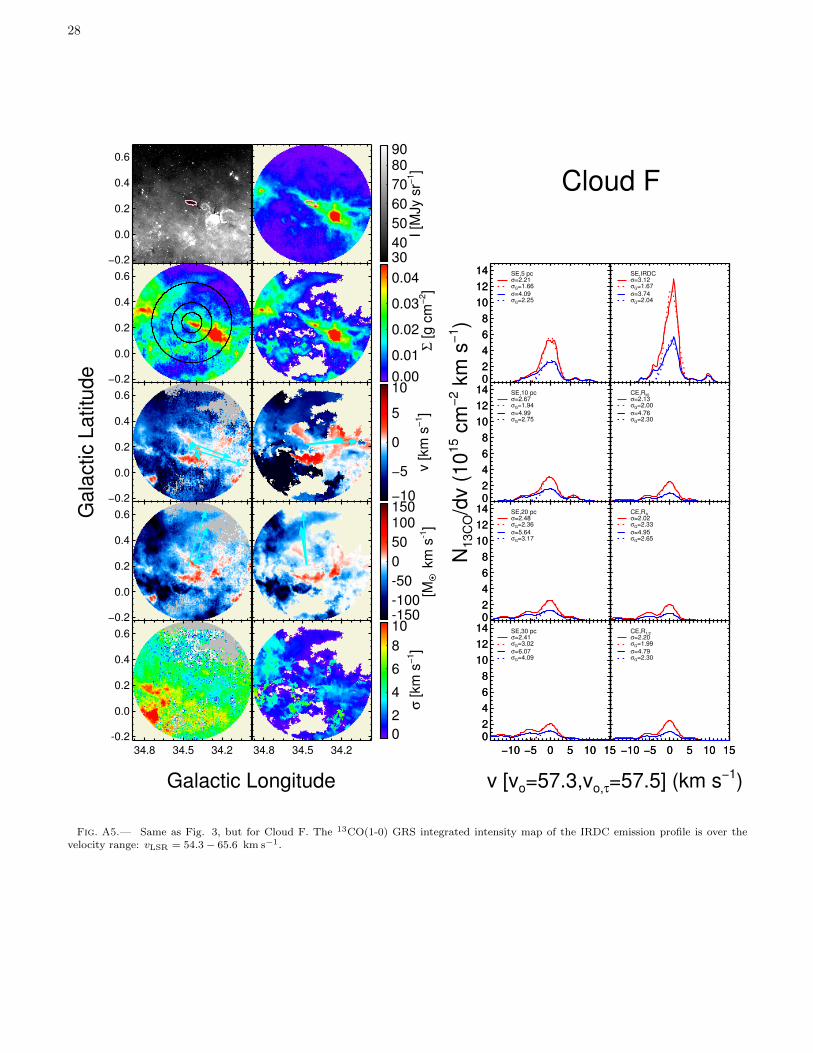
28
−0.2
0.0
0.2
0.4
0.6
3040
50
60
70
8090
I [M
Jy s
r−1]
−0.2
0.0
0.2
0.4
0.6
0.00
0.01
0.02
0.03
0.04
Σ [
g c
m−
2]
−0.2
0.0
0.2
0.4
0.6
−10
−5
0
5
10
v [
km
s−
1]
−0.2
0.0
0.2
0.4
0.6
-150-100
-50
0
50
100150
[MO •
km
s-1]
34.8 34.5 34.2
-0.2
0.0
0.2
0.4
0.6
34.8 34.5 34.2
0
2
4
6
8
10
σ [
km
s−
1]
Gala
ctic L
atitu
de
Galactic Longitude
Cloud F
02
4
6
8
10
12
14 SE,5 pcσ=2.21σG=1.66
02
4
6
8
10
12
14 SE,10 pcσ=2.67σG=1.94
02
4
6
8
10
12
14 SE,20 pcσ=2.48σG=2.36
−10 −5 0 5 10 15
02
4
6
8
10
12
14 SE,30 pcσ=2.41σG=3.02
SE,IRDCσ=3.12σG=1.67
CE,RM
σ=2.13σG=2.00
CE,RA
σ=2.02σG=2.33
−10 −5 0 5 10 15
CE,R1/2
σ=2.20σG=1.99
02
4
6
8
10
12
14
σ=4.09σG=2.25
02
4
6
8
10
12
14
σ=4.99σG=2.75
02
4
6
8
10
12
14
σ=5.64σG=3.17
−10 −5 0 5 10 15
02
4
6
8
10
12
14
σ=6.07σG=4.09
σ=3.74σG=2.04
σ=4.76σG=2.30
σ=4.95σG=2.65
−10 −5 0 5 10 15
σ=4.79σG=2.30
v [vo=57.3,vo,τ=57.5] (km s−1)
N1
3C
O/d
v (
10
15 c
m−
2 k
m s
−1)
Fig. A5.— Same as Fig. 3, but for Cloud F. The 13CO(1-0) GRS integrated intensity map of the IRDC emission profile is over thevelocity range: vLSR = 54.3− 65.6 km s−1.
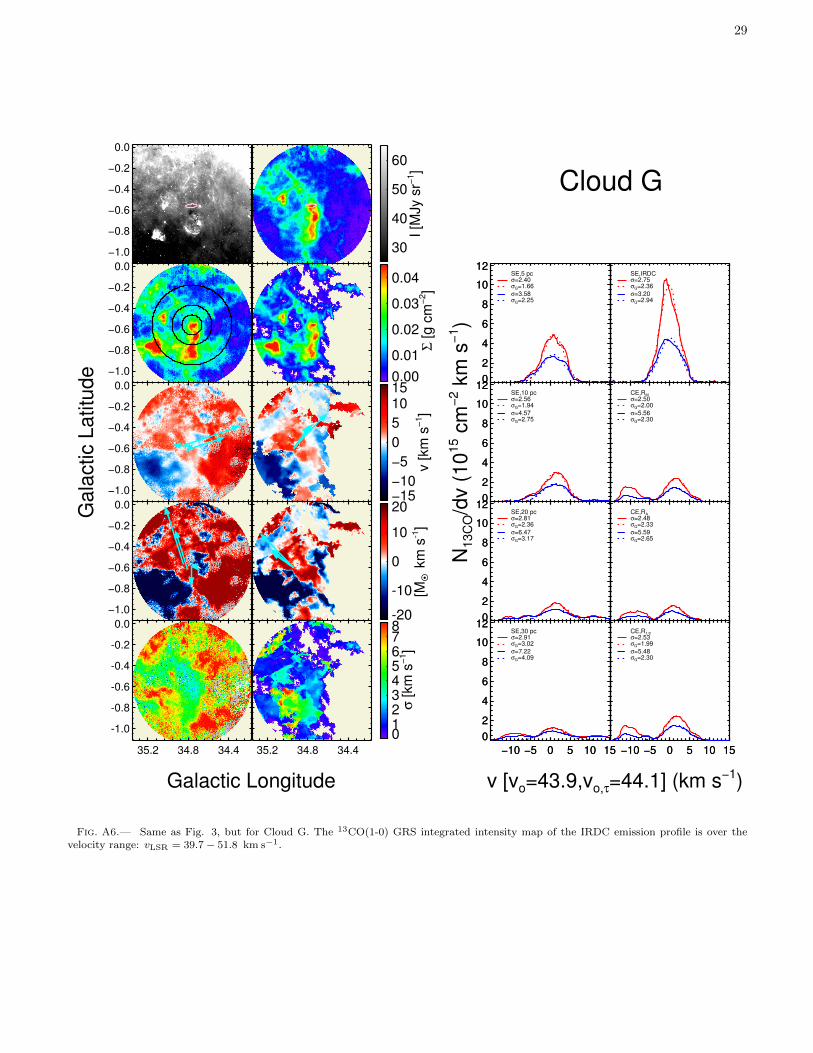
29
−1.0
−0.8
−0.6
−0.4
−0.2
0.0
30
40
50
60
I [M
Jy s
r−1]
−1.0
−0.8
−0.6
−0.4
−0.2
0.0
0.00
0.01
0.02
0.03
0.04
Σ [
g c
m−
2]
−1.0
−0.8
−0.6
−0.4
−0.2
0.0
−15−10
−5
0
5
1015
v [
km
s−
1]
−1.0
−0.8
−0.6
−0.4
−0.2
0.0
-20
-10
0
10
20
[MO •
km
s-1]
35.2 34.8 34.4
-1.0
-0.8
-0.6
-0.4
-0.2
0.0
35.2 34.8 34.4
012345678
σ [
km
s−
1]
Gala
ctic L
atitu
de
Galactic Longitude
Cloud G
0
2
4
6
8
10
12SE,5 pcσ=2.40σG=1.66
0
2
4
6
8
10
12SE,10 pcσ=2.56σG=1.94
0
2
4
6
8
10
12SE,20 pcσ=2.81σG=2.36
−10 −5 0 5 10 15
0
2
4
6
8
10
12SE,30 pcσ=2.91σG=3.02
SE,IRDCσ=2.75σG=2.36
CE,RM
σ=2.50σG=2.00
CE,RA
σ=2.48σG=2.33
−10 −5 0 5 10 15
CE,R1/2
σ=2.53σG=1.99
0
2
4
6
8
10
12
σ=3.58σG=2.25
0
2
4
6
8
10
12
σ=4.57σG=2.75
0
2
4
6
8
10
12
σ=6.47σG=3.17
−10 −5 0 5 10 15
0
2
4
6
8
10
12
σ=7.22σG=4.09
σ=3.20σG=2.94
σ=5.56σG=2.30
σ=5.59σG=2.65
−10 −5 0 5 10 15
σ=5.48σG=2.30
v [vo=43.9,vo,τ=44.1] (km s−1)
N1
3C
O/d
v (
10
15 c
m−
2 k
m s
−1)
Fig. A6.— Same as Fig. 3, but for Cloud G. The 13CO(1-0) GRS integrated intensity map of the IRDC emission profile is over thevelocity range: vLSR = 39.7− 51.8 km s−1.

30
−0.8
−0.6
−0.4
−0.2
0.0
0.2
30
40
50
60
70
I [M
Jy s
r−1]
−0.8
−0.6
−0.4
−0.2
0.0
0.2
0.00
0.01
0.02
0.03
0.04
Σ [
g c
m−
2]
−0.8
−0.6
−0.4
−0.2
0.0
0.2
−15−10
−5
0
5
1015
v [
km
s−
1]
−0.8
−0.6
−0.4
−0.2
0.0
0.2
-100
-50
0
50
100
[MO •
km
s-1]
36.0 35.7 35.4 35.1
-0.8
-0.6
-0.4
-0.2
0.0
0.2
36.0 35.7 35.4 35.1
012345678
σ [
km
s−
1]
Gala
ctic L
atitu
de
Galactic Longitude
Cloud H
0
2
4
6
8SE,5 pcσ=1.37σG=1.66
0
2
4
6
8SE,10 pcσ=1.47σG=1.94
0
2
4
6
8SE,20 pcσ=1.60σG=2.36
−10 −5 0 5 10 15
0
2
4
6
8SE,30 pcσ=1.72σG=3.02
SE,IRDCσ=5.64σG=1.42
CE,RM
σ=1.36σG=2.00
CE,RA
σ=1.44σG=2.33
−10 −5 0 5 10 15
CE,R1/2
σ=1.35σG=1.99
0
2
4
6
8σ=6.53σG=2.25
0
2
4
6
8σ=6.82σG=2.75
0
2
4
6
8σ=7.16σG=3.17
−10 −5 0 5 10 15
0
2
4
6
8σ=7.92σG=4.09
σ=6.12σG=1.68
σ=5.95σG=2.30
σ=7.41σG=2.65
−10 −5 0 5 10 15
σ=6.19σG=2.30
v [vo=47.5,vo,τ=48.0] (km s−1)
N1
3C
O/d
v (
10
15 c
m−
2 k
m s
−1)
Fig. A7.— Same as Fig. 3, but for Cloud H. The 13CO(1-0) GRS integrated intensity map of the IRDC emission profile is over thevelocity range: vLSR = 39.7− 47.1 km s−1.
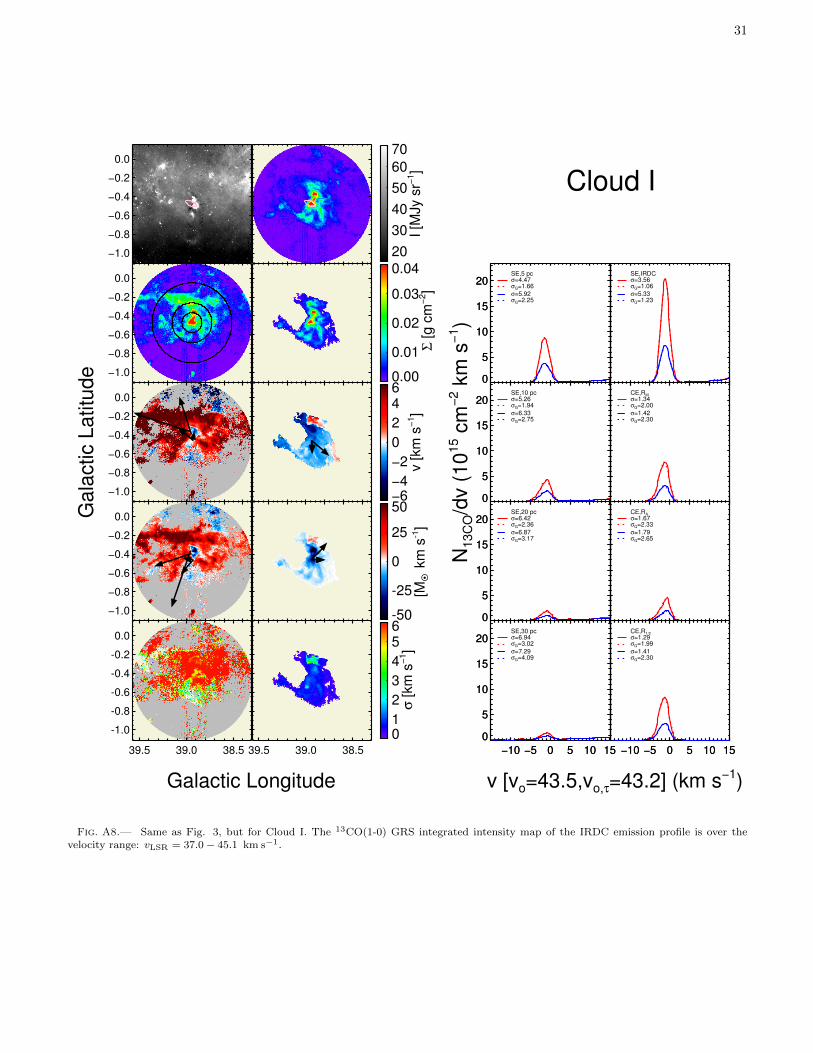
31
−1.0
−0.8
−0.6
−0.4
−0.2
0.0
20
30
40
50
60
70
I [M
Jy s
r−1]
−1.0
−0.8
−0.6
−0.4
−0.2
0.0
0.00
0.01
0.02
0.03
0.04
Σ [
g c
m−
2]
−1.0
−0.8
−0.6
−0.4
−0.2
0.0
−6−4
−2
0
2
46
v [
km
s−
1]
−1.0
−0.8
−0.6
−0.4
−0.2
0.0
-50
-25
0
25
50
[MO •
km
s-1]
39.5 39.0 38.5
-1.0
-0.8
-0.6
-0.4
-0.2
0.0
39.5 39.0 38.5
01
2
3
4
56
σ [
km
s−
1]
Gala
ctic L
atitu
de
Galactic Longitude
Cloud I
0
5
10
15
20SE,5 pcσ=4.47σG=1.66
0
5
10
15
20SE,10 pcσ=5.26σG=1.94
0
5
10
15
20SE,20 pcσ=6.42σG=2.36
−10 −5 0 5 10 15
0
5
10
15
20SE,30 pcσ=6.94σG=3.02
SE,IRDCσ=3.56σG=1.06
CE,RM
σ=1.34σG=2.00
CE,RA
σ=1.67σG=2.33
−10 −5 0 5 10 15
CE,R1/2
σ=1.29σG=1.99
0
5
10
15
20σ=5.92σG=2.25
0
5
10
15
20σ=6.33σG=2.75
0
5
10
15
20σ=6.87σG=3.17
−10 −5 0 5 10 15
0
5
10
15
20σ=7.29σG=4.09
σ=5.33σG=1.23
σ=1.42σG=2.30
σ=1.79σG=2.65
−10 −5 0 5 10 15
σ=1.41σG=2.30
v [vo=43.5,vo,τ=43.2] (km s−1)
N1
3C
O/d
v (
10
15 c
m−
2 k
m s
−1)
Fig. A8.— Same as Fig. 3, but for Cloud I. The 13CO(1-0) GRS integrated intensity map of the IRDC emission profile is over thevelocity range: vLSR = 37.0− 45.1 km s−1.

32
−0.5
0.0
0.5
1.0
15
20
25
30
I [M
Jy s
r−1]
−0.5
0.0
0.5
1.0
0.00
0.01
0.02
Σ [
g c
m−
2]
−0.5
0.0
0.5
1.0
−2
−1
0
1
2
v [
km
s−
1]
−0.5
0.0
0.5
1.0
-2
-1
0
1
2
[MO •
km
s-1]
54.0 53.5 53.0 52.5
-0.5
0.0
0.5
1.0
54.0 53.5 53.0 52.5
0.0
0.5
1.0
1.5
2.0
σ [
km
s−
1]
Gala
ctic L
atitu
de
Galactic Longitude
Cloud J
0
5
10
15
20SE,5 pcσ=4.61σG=1.66
0
5
10
15
20SE,10 pcσ=4.42σG=1.94
0
5
10
15
20SE,20 pcσ=4.17σG=2.36
−10 −5 0 5 10 15
0
5
10
15
20SE,30 pcσ=4.59σG=3.02
SE,IRDCσ=1.75σG=0.73
CE,RM
σ=1.06σG=2.00
CE,RA
σ=1.08σG=2.33
−10 −5 0 5 10 15
CE,R1/2
σ=1.06σG=1.99
0
5
10
15
20
σ=5.44σG=2.25
0
5
10
15
20
σ=5.16σG=2.75
0
5
10
15
20
σ=4.87σG=3.17
−10 −5 0 5 10 15
0
5
10
15
20
σ=5.28σG=4.09
σ=2.30σG=0.83
σ=1.10σG=2.30
σ=1.11σG=2.65
−10 −5 0 5 10 15
σ=1.08σG=2.30
v [vo=21.4,vo,τ=21.6] (km s−1)
N1
3C
O/d
v (
10
15 c
m−
2 k
m s
−1)
Fig. A9.— Same as Fig. 3, but for Cloud J. The 13CO(1-0) GRS integrated intensity map of the IRDC emission profile is over thevelocity range: vLSR = 18.7− 27.1 km s−1.

33
REFERENCES
Anderson, L. D., Bania, T. M., Balser, D. S., et al. 2014, ApJS,212, 1
Battersby, C., & Bally, J. 2012, ArXiv e-prints, arXiv:1208.4608Battersby, C., Bally, J., Jackson, J. M., et al. 2010, ApJ, 721, 222Benjamin, R. A., Churchwell, E., Babler, B. L., et al. 2003, PASP,
115, 953Bertoldi, F., & McKee, C. F. 1992, ApJ, 395, 140Blitz, L. 1993, in Protostars and Planets III, ed. E. H. Levy &
J. I. Lunine, 125–161Brunthaler, A., Reid, M. J., Menten, K. M., et al. 2009, ApJ, 693,
424Burkert, A., & Bodenheimer, P. 2000, ApJ, 543, 822Butler, M. J., & Tan, J. C. 2009, ApJ, 696, 484—. 2012, ApJ, 754, 5Butler, M. J., Tan, J. C., & Kainulainen, J. 2014, ApJ, 782, L30Carey, S. J., Clark, F. O., Egan, M. P., et al. 1998, ApJ, 508, 721Carey, S. J., Feldman, P. A., Redman, R. O., et al. 2000, ApJ,
543, L157Chira, R.-A., Beuther, H., Linz, H., et al. 2013, A&A, 552, A40Clemens, D. P. 1985, ApJ, 295, 422Crutcher, R. M. 2012, ARA&A, 50, 29Dame, T. M., Hartmann, D., & Thaddeus, P. 2001, ApJ, 547, 792Devine, K. 2009, PhD thesis, University of WisconsinDobbs, C. L., Burkert, A., & Pringle, J. E. 2011, MNRAS, 417,
1318Dobbs, C. L., & Pringle, J. E. 2013, MNRAS, 432, 653Egan, M. P., Shipman, R. F., Price, S. D., et al. 1998, ApJ, 494,
L199+Fontani, F., Caselli, P., Crapsi, A., et al. 2006, A&A, 460, 709Foster, J. B., Rosolowsky, E. W., Kauffmann, J., et al. 2009, ApJ,
696, 298Foster, J. B., Stead, J. J., Benjamin, R. A., Hoare, M. G., &
Jackson, J. M. 2012, ApJ, 751, 157Goldsmith, P. F., Heyer, M., Narayanan, G., et al. 2008, ApJ,
680, 428Goodman, A. A., Benson, P. J., Fuller, G. A., & Myers, P. C.
1993, ApJ, 406, 528Heitsch, F., Slyz, A. D., Devriendt, J. E. G., Hartmann, L. W., &
Burkert, A. 2006, ApJ, 648, 1052Henshaw, J. D., Caselli, P., Fontani, F., Jimenez-Serra, I., & Tan,
J. C. 2014, MNRAS, 440, 2860Henshaw, J. D., Caselli, P., Fontani, F., et al. 2013, MNRAS, 428,
3425Hernandez, A. K., & Tan, J. C. 2011, ApJ, 730, 44Hernandez, A. K., Tan, J. C., Caselli, P., et al. 2011, ApJ, 738, 11Hernandez, A. K., Tan, J. C., Kainulainen, J., et al. 2012, ApJ,
756, L13Heyer, M., Krawczyk, C., Duval, J., & Jackson, J. M. 2009, ApJ,
699, 1092Imara, N., Bigiel, F., & Blitz, L. 2011, ApJ, 732, 79Imara, N., & Blitz, L. 2011, ApJ, 732, 78Jackson, J. M., Finn, S. C., Chambers, E. T., Rathborne, J. M.,
& Simon, R. 2010, ApJ, 719, L185Jackson, J. M., Rathborne, J. M., Shah, R. Y., et al. 2006, ApJS,
163, 145Jimenez-Serra, I., Caselli, P., Fontani, F., et al. 2014, MNRAS,
439, 1996Jimenez-Serra, I., Caselli, P., Tan, J. C., et al. 2010, MNRAS,
406, 187Kainulainen, J., & Tan, J. C. 2013, A&A, 549, A53Kirk, H., Pineda, J. E., Johnstone, D., & Goodman, A. 2010,
ApJ, 723, 457Koda, J., Sawada, T., Hasegawa, T., & Scoville, N. Z. 2006, ApJ,
638, 191Krumholz, M. R., & McKee, C. F. 2005, ApJ, 630, 250Krumholz, M. R., & Tan, J. C. 2007, ApJ, 654, 304Kurayama, T., Nakagawa, A., Sawada-Satoh, S., et al. 2011,
PASJ, 63, 513Lacy, J. H., Knacke, R., Geballe, T. R., & Tokunaga, A. T. 1994,
ApJ, 428, L69Lada, C. J., & Lada, E. A. 2003, ARA&A, 41, 57Lada, C. J., Lombardi, M., & Alves, J. F. 2010, ApJ, 724, 687Larson, R. B. 1981, MNRAS, 194, 809
Li, H.-B., Goodman, A., Sridharan, T. K., et al. 2014, Protostarsand Planets VI, 101
McKee, C. F. 1989, ApJ, 345, 782McKee, C. F., Li, P. S., & Klein, R. I. 2010, ApJ, 720, 1612McKee, C. F., & Ostriker, E. C. 2007, ARA&A, 45, 565McKee, C. F., & Tan, J. C. 2003, ApJ, 585, 850Milam, S. N., Savage, C., Brewster, M. A., Ziurys, L. M., &
Wyckoff, S. 2005, ApJ, 634, 1126Mouschovias, T. 2001, in Astronomical Society of the Pacific
Conference Series, Vol. 248, Magnetic Fields Across theHertzsprung-Russell Diagram, ed. G. Mathys, S. K. Solanki, &D. T. Wickramasinghe, 515
Nguyen-Lu’o’ng, Q., Motte, F., Carlhoff, P., et al. 2013, ApJ, 775,88
Padoan, P., & Nordlund, A. 2011, ApJ, 730, 40Perault, M., Omont, A., Simon, G., et al. 1996, A&A, 315, L165Peretto, N., & Fuller, G. A. 2009, A&A, 505, 405Peretto, N., Fuller, G. A., Plume, R., et al. 2010, A&A, 518, L98Peretto, N., Fuller, G. A., Duarte-Cabral, A., et al. 2013, A&A,
555, A112Phillips, J. P. 1999, A&AS, 134, 241Pillai, T., Kauffmann, J., Tan, J. C., et al. 2015, ApJ, 799, 74Pillai, T., Wyrowski, F., Carey, S. J., & Menten, K. M. 2006,
A&A, 450, 569Ragan, S. E., Bergin, E. A., & Wilner, D. 2011, ApJ, 736, 163Ragan, S. E., Heitsch, F., Bergin, E. A., & Wilner, D. 2012, ApJ,
746, 174Ragan, S. E., Henning, T., Tackenberg, J., et al. 2014, A&A, 568,
A73Rathborne, J. M., Jackson, J. M., & Simon, R. 2006, ApJ, 641,
389Rathborne, J. M., Johnson, A. M., Jackson, J. M., Shah, R. Y., &
Simon, R. 2009, ApJS, 182, 131Reid, M. J., Menten, K. M., Brunthaler, A., et al. 2014, ApJ, 783,
130Ridge, N. A., Di Francesco, J., Kirk, H., et al. 2006, AJ, 131, 2921Roman-Duval, J., Jackson, J. M., Heyer, M., et al. 2009, ApJ,
699, 1153Roman-Duval, J., Jackson, J. M., Heyer, M., Rathborne, J., &
Simon, R. 2010, ApJ, 723, 492Rosolowsky, E., Engargiola, G., Plambeck, R., & Blitz, L. 2003,
ApJ, 599, 258Samal, M. R., Zavagno, A., Deharveng, L., et al. 2014, A&A, 566,
A122Sanhueza, P., Jackson, J. M., Foster, J. B., et al. 2013, ApJ, 773,
123Scoville, N. Z., Sanders, D. B., & Clemens, D. P. 1986, ApJ, 310,
L77Shimajiri, Y., Kawabe, R., Takakuwa, S., et al. 2011, PASJ, 63,
105Simon, R., Jackson, J. M., Bania, T. M., et al. 2001, in Bulletin
of the American Astronomical Society, Vol. 33, AmericanAstronomical Society Meeting Abstracts, 1450–+
Simon, R., Jackson, J. M., Rathborne, J. M., & Chambers, E. T.2006a, ApJ, 639, 227
Simon, R., Rathborne, J. M., Shah, R. Y., Jackson, J. M., &Chambers, E. T. 2006b, ApJ, 653, 1325
Solomon, P. M., Rivolo, A. R., Barrett, J., & Yahil, A. 1987, ApJ,319, 730
Tan, J. C. 2000, ApJ, 536, 173Tan, J. C., Beltran, M. T., Caselli, P., et al. 2014, Protostars and
Planets VI, 149Tan, J. C., Shaske, S. N., & Van Loo, S. 2013, in IAU Symposium,
Vol. 292, IAU Symposium, ed. T. Wong & J. Ott, 19–28Tasker, E. J., & Tan, J. C. 2009, ApJ, 700, 358Wienen, M., Wyrowski, F., Schuller, F., et al. 2012, A&A, 544,
A146Williams, J. P., Blitz, L., & McKee, C. F. 2000, Protostars and
Planets IV, 97Williams, J. P., de Geus, E. J., & Blitz, L. 1994, ApJ, 428, 693Zuckerman, B., & Evans, II, N. J. 1974, ApJ, 192, L149