Embed Size (px)
Citation preview
Hindawi Publishing CorporationMathematical Problems in EngineeringVolume 2013 Article ID 548487 8 pageshttpdxdoiorg1011552013548487
Research ArticleAugmented Arnoldi-Tikhonov Regularization Methods forSolving Large-Scale Linear Ill-Posed Systems
Yiqin Lin1 Liang Bao2 and Yanhua Cao3
1 Department of Mathematics and Computational Science Hunan University of Science and Engineering Yongzhou 425100 China2Department of Mathematics East China University of Science and Technology Shanghai 200237 China3Department of Mathematics North China Electric Power University Beijing 102206 China
Correspondence should be addressed to Liang Bao nlbaoyahoocn
Received 1 November 2012 Revised 18 March 2013 Accepted 19 March 2013
Academic Editor Hung Nguyen-Xuan
Copyright copy 2013 Yiqin Lin et alThis is an open access article distributed under the Creative CommonsAttribution License whichpermits unrestricted use distribution and reproduction in any medium provided the original work is properly cited
We propose an augmented Arnoldi-Tikhonov regularization method for the solution of large-scale linear ill-posed systems Thismethod augments the Krylov subspace by a user-supplied low-dimensional subspace which contains a rough approximation ofthe desired solution The augmentation is implemented by a modified Arnoldi process Some useful results are also presentedNumerical experiments illustrate that the augmented method outperforms the corresponding method without augmentation onsome real-world examples
1 Introduction
We consider the iterative solution of a large system of linearequations
119860119909 = 119887 (1)
where 119860 isin R119899times119899 is nonsymmetric and nonsingular and119887 isin R119899 We further assume that the coefficient matrix 119860 isof ill-determined rank that is all its singular values decaygradually to zero with no gap anywhere in the spectrumSuch systems are often referred to as linear discrete ill-posed problems and arise from the discretization of ill-posedproblems such as Fredholm integral equations of the first kindwith a smooth kernelThe right-hand side 119887 of (1) is assumedto be contaminated by an error 119890 isin R119899 which may stem fromdiscretization or measurement inaccuracies Thus 119887 = + 119890where is the unknown error-free right-hand side vector
We would like to compute the solution 119909 of the linearsystem of equations with the error-free right-hand side
119860119909 = (2)
However since the right-hand side in (2) is not availablewe seek to determine an approximation of 119909 by solving the
available system (1) or a modification Due to the ill condi-tioning of 119860 the system (1) has to be regularized in orderto compute a useful approximation of 119909 Perhaps the bestknown regularization method is Tikhonov regularization [1ndash3] which in its simplest form is based on the minimizationproblem
min119909isinR119899
119860119909 minus 1198872
+1
1205831199092
(3)
where 120583 gt 0 is a regularization parameter Here andthroughout this paper sdot denotes the Euclidean vectornorm or the associated induced matrix norm
After regulating the system (1) we need to compute thesolution 119909
120583of the minimization problem (3) Such a vector
119909120583is also the solution of
(119860119879
119860 +1
120583119868)119909 = 119860
119879
119887 (4)
Here and in the following 119868 denotes the identity matrixwhose dimension is conformed with the dimension used inthe context If 120583 is far away from zero then due to theill conditioning of 119860 119909
120583is badly computed while if 120583 is
close to zero 119909120583is well computed but the error 119909
120583minus 119909 is
2 Mathematical Problems in Engineering
quite large Thus the choice of a good value for 120583 is fairlyimportant Several methods have been proposed to obtain aneffective value for 120583 For example if the norm of the error119890 or a fairly accurate estimate is known the regularizationparameter is quite easy to determine by application of thediscrepancy principle The discrepancy principle proposesthat the regularization parameter 120583 can be chosen so that thediscrepancy 119887 minus 119860119909
120583satisfies
10038171003817100381710038171003817119887 minus 119860119909
120583
10038171003817100381710038171003817= 120578120576 (5)
where 120576 = 119890 and 120578 gt 1 is a constant see for example [4]for further details on the discrepancy principle
The singular value decomposition [5] of 119860 can be usedto determine the solution 119909
120583of the minimization problem
(3) For an overview of numerical methods for computingthe SVD we refer to [6] We remark that the computationaleffort required to compute the SVD is quite high even formoderately sized matrices
Many numerical methods using Krylov subspaces havebeen proposed for the solution of large-scale Tikhonovregularization problems (3)Themain idea of such algorithmshas been to first project the large problems onto some Krylovsubspace to produce problems with small size and then solvethe small-sized problems by the SVD For instance severalwell-established methods based on the Lanczos bidiagonal-ization process have been proposed for the solution of theminimization problem (3) see [7ndash10] and references thereinThese methods use the Lanczos bidiagonalization process toconstruct a basis of the Krylov subspace
K119898(119860119879
119860119860119879
119887)
= span 119860119879119887 119860119879119860119860119879119887 (119860119879119860)119898minus1
119860119879
119887
(6)
We remark that each Lanczos bidiagonalization step needstwo matrix-vector product evaluations one with 119860 and theother with 119860119879 Other methods using the Krylov subspace
K119898(119860 119860119887) = span 119860119887 1198602119887 119860119898119887 (7)
as the projection subspace have been also designed Forexample Lewis and Reichel [11] proposed to exploit theArnoldi process to produce a basis of the Krylov subspaceK119898(119860 119860119887) to obtain an approximation of the solution of
the Tikhonov regularization problem (3) Since each Arnoldidecomposition step requires only one matrix-vector evalua-tion with 119860 the approach based on the Arnoldi process mayrequire fewer matrix-vector product evaluations than thatbased on the Lanczos bidiagonalization process Moreoverthe methods based on the Arnoldi process do not requirethe adjoint matrix 119860119879 and hence are more appropriateto problems for which the adjoint is difficult to evaluateFor such problems we refer to [12] A similar Tikhonovregularizationmethod based on generalized Krylov subspaceis proposed in [13]
Some numerical methods without using the Tikhonovregularization technique have been already proposed to solvethe large-scale linear discrete ill-posed problem (1) Thesemethods include the range-restricted GMRES (RRGMRES)method [14 15] the augmented range-restricted GMRES(ARRGMRES) method [16] and the flexible GMRES (FGM-RES) method [17] The RRGMRES method determines the119898th approximation 119909
119898of (1) by solving the minimization
problem
min119909isinK119898(119860119860119887)
119860119909 minus 119887 119898 = 1 2 1199090= 0 (8)
The regularization is implemented by choosing a suitabledimension number 119898 see for example [18] The ARRGM-RES method augments the Krylov subspace K
119898(119860 119860119887)
by a low-dimensional user-supplied subspace The low-dimensional subspace is determined by vectors that are ableto represent the known features of the desired solutionThe augmented method can yield approximate solutions ofhigher accuracy than the RRGMRES method if the Krylovsubspace K
119898(119860 119860119887) does not allow representation of the
known featuresIn this paper we propose a new iterative method named
augmented Arnoldi-Tikhonov regularization method forsolving large-scale linear ill-posed systems (1) The newmethod is deduced by combining the Tikhonov regulariza-tion technique and the augmentation technique The aug-mentation is implemented by a modified Arnoldi process
The following summarizes the structure of this paperSection 2 describes the augmented Arnoldi-Tikhonov regu-larization method and some useful results Some real-worldexamples are presented in Section 3 Section 4 contains theconclusions
2 Augmented Arnoldi-TikhonovRegularization Method
We attempt to improve the Arnoldi-Tikhonov regularizationmethod proposed in [11] by augmenting the Krylov subspaceK119898(119860 119860119887) by a 119896-dimensional subspaceW which contains
a rough approximation of the desired solution of (2) Thenthe subspace of projection we will exploit in the following isof the form
K119898(119860 119860119887) +W = span 119860119887 1198602119887 119860119898119887 +W (9)
Let 119882 be the 119899 by 119896 matrix whose columns form anorthonormal basis of the space W For the purpose ofaugmentation by W we apply the modified Arnoldi process[16] to construct the modified Arnoldi decomposition
119860 [119882119881119898] = [119880 119881
119898+1]119867 (10)
where 119880 isin R119899times119896 119881119898+1
isin R119899times(119898+1) [119880 119881119898+1] has orthonor-
mal columns and119867 isin R(119898+119896+1)times(119898+119896) is an upperHessenbergmatrix We point out that the leading principal 119896 by 119896submatrix of 119867 is the upper triangular matrix in the QRfactorization [5] of 119860119882 that is119867 is of the form
Mathematical Problems in Engineering 3
Input 119860 isin R119899times119899 119887 isin R119899119882 isin R119899times119896119898Output 119880 isin R119899times119896 119881
119898+1isin R119899times(119898+1)119867 isin R(119898+119896+1)times(119898+119896)
(1) Compute QR-factorization 119860119882 = 119880119867(2) Compute V
1= 119860119887 minus 119880(119880
119879
119860119887) V1= V11003817100381710038171003817V11003817100381710038171003817 and set 119881
1= [V1]
(3) For 119895 = 1 2 119898 DoV119895+1= 119860V
119895
For 119894 = 1 2 119896 Doℎ119894119895+119896
= 119880( 119894)119879
V119895+1
V119895+1= V119895+1minus ℎ119894119895+119896119880( 119894)
End ForFor 119894 = 1 2 119895 Do
ℎ119894+119896119895+119896
= V119879119894V119895+1
V119895+1= V119895+1minus ℎ119894+119896119895+119896
V119894
End Forℎ119895+119896+1119895+119896
= V119895+110038171003817100381710038171003817V119895+1
10038171003817100381710038171003817
V119895+1= V119895+1ℎ119895+119896+1119895+119896
119881119895+1= [119881119895 V119895+1]
End For
Algorithm 1 Modified Arnoldi process
119867 =
[[[[[[[[[[[[[[[
[
ℎ11ℎ12
sdot sdot sdot ℎ1119896
ℎ1119896+1
ℎ1119896+2
sdot sdot sdot ℎ1119896+119898
d d
sdot sdot sdot
ℎ119896minus1119896minus1
ℎ119896minus1119896
ℎ119896minus1119896+1
ℎ119896minus1119896+2
sdot sdot sdot ℎ119896minus1119896+119898
ℎ119896119896
ℎ119896119896+1
ℎ119896119896+2
sdot sdot sdot ℎ119896119896+119898
ℎ119896+1119896+1
ℎ119896+1119896+2
sdot sdot sdot ℎ119896+1119896+119898
ℎ119896+2119896+1
ℎ119896+2119896+2
sdot sdot sdot ℎ119896+2119896+119898
d d
ℎ119896+119898119896+119898minus1
ℎ119896+119898119896+119898
ℎ119896+119898+1119896+119898
]]]]]]]]]]]]]]]
]
(11)
ThemodifiedArnoldi relation (10) is shared by othermethodssuch as GMRES-E [19] and FGMRES [20] which are alsoaugmented type methods
The modified Arnoldi process is outlined in Algorithm 1We remark that the modified Arnoldi process in this paperis slightly different from the one used by Morgan [19]to augment the Krylov subspace with some approximateeigenvectors In his method the augmenting vectors are putafter the Krylov vectors while in Algorithm 1 the augment-ing subspace containing a rough approximation solution isincluded in the projection subspace from the beginningIn general this can give better results at the start of theregularization method proposed in this paper
We remark that a loss of orthogonality can occur whenthe algorithm progresses see [21] A remedy is the so-called reorthogonalization where the current vector has tobe orthogonalized against previously created vectors Onecan choose between a selective reorthogonalization or a full
reorthogonalization against all vectors in the current aug-mented subspace In this paper we only use the full reorthog-onalization The full reorthogonalization can be done as aclassical or modifed Gram-Schmidt orthogonalization see[21] for details
We now seek to determine an approximate solution 119909120583119898
of (3) in the augmented Krylov subspace K119898(119860 119860119887) +W
After computing theQR factorization [119882119881119898] = 119876119877with119876 isin
R119899times(119898+119896) having orthonormal columns and 119877 isin R(119898+119896)times(119898+119896)
being an upper triangularmatrix we substitute119909 = [119882119881119898]119910
119910 isin R119898+119896 into (3) It yields the reduced minimizationproblem
min119910isinR119898+119896
1003817100381710038171003817119860 [119882119881119898] 119910 minus 119887
1003817100381710038171003817
2
+1
120583
1003817100381710038171003817[119882119881119898] 1199101003817100381710038171003817
2
= min119910isinR119898+119896
1003817100381710038171003817[119880 119881119898+1]119867119910 minus 119887
1003817100381710038171003817
2
+1
120583
10038171003817100381710038171198761198771199101003817100381710038171003817
2
4 Mathematical Problems in Engineering
= min119910isinR119898+119896
10038171003817100381710038171003817119867119910 minus [119880119881
119898+1]119879
11988710038171003817100381710038171003817
2
+(119868 minus 119875)1198872
+1
120583
10038171003817100381710038171198771199101003817100381710038171003817
2
(12)
in which 119875 = [119880119881119898+1][119880 119881
119898+1]119879 is an orthogonal projector
onto span([119880 119881119898+1]) Obviously the reduced minimization
problem (12) is equivalent to
min119910isinR119898+119896
10038171003817100381710038171003817119867119910 minus [119880119881
119898+1]119879
11988710038171003817100381710038171003817
2
+1
120583
10038171003817100381710038171198771199101003817100381710038171003817
2
= min119910isinR119898+119896
100381710038171003817100381710038171003817100381710038171003817100381710038171003817
[
[
119867
1
radic120583119877]
]
119910 minus [[119880119881119898+1]119879
119887
0]
100381710038171003817100381710038171003817100381710038171003817100381710038171003817
2
(13)
The normal equations of the minimization problem (13) is
(119867119879
119867 +1
120583119877119879
119877)119910 = 119867119879
[119880 119881119898+1]119879
119887 (14)
We denote the solution of the minimization problem (13) by119910120583119898
Then from (14) it follows that
119910120583119898= (119867
119879
119867 +1
120583119877119879
119877)
minus1
119867119879
[119880 119881119898+1]119879
119887 (15)
The approximate solution of (3) is
119909120583119898= [119882119881
119898] 119910120583119898 (16)
Since the matrix119867119879119867+ (1120583)119877119879119877 has a larger conditionnumber than the matrix [119867119879 (1radic120583)119877119879]119879 we apply the QRfactorization of [119867119879 (1radic120583)119877119879]119879 to obtain the solution 119910
120583119898
of (13) insteadTheQR factorization of [119867119879 (1radic120583)119877119879]119879 canbe implemented by a sequence of Givens rotations
Define
120601119898(120583) =
10038171003817100381710038171003817119887 minus 119860119909
120583119898
10038171003817100381710038171003817
2
(17)
Substituting 119909120583119898
= [119882119881119898]119910120583119898
into (17) and using themodified Arnoldi decomposition (10) yield
120601119898(120583) =
10038171003817100381710038171003817119887 minus 119860 [119882119881
119898] 119910120583119898
10038171003817100381710038171003817
2
=10038171003817100381710038171003817119887 minus [119880119881
119898+1]119867119910120583119898
10038171003817100381710038171003817
2
=10038171003817100381710038171003817[119880 119881119898+1]119879
119887 minus 119867119910120583119898
10038171003817100381710038171003817
2
+ (119868 minus 119875)1198872
(18)
Substituting 119910120583119898
in (15) into (18) we obtain
120601119898(120583) =
100381710038171003817100381710038171003817100381710038171003817
[119868 minus 119867(119867119879
119867 +1
120583119877119879
119877)
minus1
119867119879
] [119880119881119898+1]119879
119887
100381710038171003817100381710038171003817100381710038171003817
2
+ (119868 minus 119875) 1198872
(19)
Note that
119868 minus 119867(119867119879
119867 +1
120583119877119879
119877)
minus1
119867119879
= [120583119867119877minus1
(119867119877minus1
)119879
+ 119868]
minus1
(20)
Therefore the function 120601119898(120583) can be expressed as
120601119898(120583) =
10038171003817100381710038171003817100381710038171003817
[120583119867119877minus1
(119867119877minus1
)119879
+ 119868]
minus1
[119880 119881119898+1]119879
119887
10038171003817100381710038171003817100381710038171003817
2
+ (119868 minus 119875) 1198872
(21)
Concerning the properties of 120601119898(120583) we have the follow-
ing results which are similar to those of Theorem 21 in [11]for the Arnoldi-Tikhonov regularization method
Theorem 1 The function 120601119898(120583) has the representation
120601119898(120583) = 119887
119879
[119880 119881119898+1] [120583119867119877
minus1
(119867119877minus1
)119879
+ 119868]
minus2
times [119880119881119898+1]119879
119887 + (119868 minus 119875) 1198872
(22)
Assume that 119860119887 = 0 and (119867119877minus1)119879[119880 119881119898+1]119879
119887 = 0 Then 120601119898is
strictly decreasing and convex for 120583 ge 0 with 120601119898(0) = 119887
2Moreover the equation
120601119898(120583) = 120591 (23)
has a unique solution 120583120591119898
such that 0 lt 120583120591119898lt infin for any 120591
with100381710038171003817100381710038171003817119875N((119867119877minus1)119879)[119880 119881119898+1]
119879
119887100381710038171003817100381710038171003817
2
+ (119868 minus 119875) 1198872
lt 120591 lt 1198872
(24)
where 119875N((119867119877minus1)119879) denotes the orthogonal projector ontoN((119867119877minus1)
119879
)
Proof The proof follows the same argument of the proof ofTheorem 21 in [11] and therefore is omitted
We easily obtain the following theorem of which theproof is almost the same as that of Corollary 22 in [11]
Theorem 2 Assume that the modified Arnoldi process breaksdown at step 119895 Then the sequence 119904
119894119895
119894=0defined by
1199040= 1198872
119904119894=100381710038171003817100381710038171003817119875N((119867119877minus1)
119879
)[119880 119881119898+1]119879
119887100381710038171003817100381710038171003817
2
+ (119868 minus 119875)1198872
0 lt 119894 lt 119895
119904119895= 0
(25)
is decreasing
We apply the discrepancy principle to the discrepancy 119887minus119860119909120583119898
to determine an appropriate regularization parameter120583 so that it satisfies (5) To make the equation
120601119898(120583) = 120578
2
1205762 (26)
Mathematical Problems in Engineering 5
Input 119860 isin R119899times119899 119887 isin R119899119882 isin R119899times119896 120576 1205781198980
Output 119909120583119898
120583119898119898 = 119898min + 1198980
(1) Compute the modified Arnoldi decomposition 119860[119882119881119898] = [119880 119881
119898+1]119867 with119898 = 119898min + 1198980
where119898min is the smallest number such that (119868 minus 119875)1198872 lt 12057821205762(2) Compute the solution 120583
119898of the equation 120601
119898(120583) = 120578
2
1205762 by Newtonrsquos method
(3) Compute the solution 119910120583119898
of the least-squares problem (13) and obtain the approximatesolution 119909
120583119898= [119882119881
119898]119910120583119898
Algorithm 2 Augmented Arnoldi-Tikhonov regularization method
have a solution it follows from Theorem 1 that the inputparameter 119898 of the modified Arnoldi should be chosen sothat 119904
119898lt 1205782
1205762 To simplify the computations we ignore
the first term in 119904119898 Then the smallest iterative step number
denoted by 119898min of the modified Arnoldi process is chosenso that
(119868 minus 119875) 1198872
lt 1205782
1205762
(27)
We can improve the quality of the computed solution bychoosing the practical iterative step number 119898 somewhatlarger than119898min
After choosing the number 119898 of the modified Arnoldiiterative steps the regularization parameter 120583
119898is determined
by solving the nonlinear equation 120601119898(120583) = 120578
2
1205762 Many
numerical methods have been proposed for the solutionof a nonlinear equation including Newtonrsquos method [22]super-Newtonrsquos [23] method and Halleyrsquos method [24] Forthe specific nonlinear equation 120601
119898(120583) = 120578
2
1205762 Reichel and
Shyshkov proposed a new zero-finder method in their newpaper [25] In this paper we still make use of Newtonrsquosmethod to obtain the regularization parameter 120583
119898
In Algorithm 2 we outline the augmented Arnoldi-Tikhonov regularizationmethod which is used to solve large-scale linear ill-posed systems (1)
Newtonrsquos method requires to evaluate 120601119898(120583) and its first
derivative with respect to 120583 for computing approximations120583(119895)
119898of 120583119898for 119895 = 0 1 2 Let
119911120583119898= [120583119867119877
minus1
(119867119877minus1
)119879
+ 119868]
minus1
[119880 119881119898+1]119879
119887 (28)
that is 119911120583119898
satisfies the system of linear equations
[120583119867119877minus1
(119867119877minus1
)119879
+ 119868] 119911 = [119880119881119898+1]119879
119887 (29)
Note that the above linear system is the normal equations ofthe least-squares problem
min119911isinR119898+119896+1
1003817100381710038171003817100381710038171003817100381710038171003817
[12058312
(119867119877minus1
)119879
119868] 119911 minus [
0
(U 119881119898+1)119879
119887]
1003817100381710038171003817100381710038171003817100381710038171003817
(30)
For numerical stability we compute the vector 119911120583119898
by solvingthe least-squares problem Then the 120601
119898(120583) is evaluated by
computing
120601119898(120583) = 119911
119879
120583119898119911120583119898+ (119868 minus 119875) 119887
2
(31)
It is easy to show that the first derivative of 1206011015840119898(120583) can be
written as
1206011015840
119898(120583) = minus2119911
119879
120583119898119908120583119898 (32)
where
119908120583119898= [120583119867119877
minus1
(119867119877minus1
)119879
+ 119868]
minus1
119867119877minus1
(119867119877minus1
)119879
119911120583119898 (33)
Hence we may compute 119908120583119898
by solving a least-squaresproblem analogous to the above with the vector [119880 119881
119898+1]119879
119887
replaced by119867119877minus1(119867119877minus1)119879119911120583119898
The algorithm for implementing the Newton iteration for
solving the nonlinear equation 120601119898(120583) = 120578
2
1205762 is presented in
Algorithm 3Let 119909119898be the 119898th iterate produced by the augmented
RRGMRES in [16] Then 119909119898satisfies
1003817100381710038171003817119860119909119898 minus 1198871003817100381710038171003817
2
= min119909isinK119898(119860119860119887)+W
119860119909 minus 1198872
= min119910isinR119898+119896
1003817100381710038171003817119860 [119882119881119898] 119910 minus 1198871003817100381710038171003817
2
= min119910isinR119898+119896
1003817100381710038171003817[119880 119881119898+1]119867119910 minus 1198871003817100381710038171003817
2
= min119910isinR119898+119896
10038171003817100381710038171003817119867119910 minus [119880119881
119898+1]119879
11988710038171003817100381710038171003817
2
+ (119868 minus 119875)1198872
(34)
As 120583 rarr infin the reduced minimization problem (12) is thesame as the above minimization problem which shows that
119909119898= lim120583rarrinfin
119909120583119898 (35)
Therefore we obtain the following result
Theorem 3 Let 119909119898
be the 119898th iterate determined by aug-mented RRGMRES applied to (1) with initial iterate 119909
0= 0
Then1003817100381710038171003817119860119909119898 minus 119887
1003817100381710038171003817
2
= 120601119898(infin) (36)
3 Numerical Experiments
In this section we present some numerical examplesto illustrate the performance of the augmented Arnoldi-Tikhonov regularization method for the solution of large-scale linear ill-posed systems We compare the augmented
6 Mathematical Problems in Engineering
(1) Set 1205830= 0 and 119894 = 0
(2) Solve the least-squares problem
min119911isinR119898+119896+1
10038171003817100381710038171003817100381710038171003817
[12058312
119894(119867119877minus1
)119879
119868] 119911 minus [
0
(119880119881119898+1)119879
119887]
10038171003817100381710038171003817100381710038171003817
to obtain 119911120583119894119898
(3) Compute 120601119898(120583119894) = 119911119879
120583119894119898119911120583119894119898+ (119868 minus 119875)119887
2(4) Solve the least-squares problem
min119911isinR119898+119896+1
100381710038171003817100381710038171003817100381710038171003817
[12058312
119894(119867119877minus1
)119879
119868] 119911 minus [
0
119867119877minus1
(119867119877minus1
)119879
119911120583119894119898
]
100381710038171003817100381710038171003817100381710038171003817to obtain 119908
120583119894119898
(5) Compute 1206011015840119898(120583119894) = minus2119911
119879
120583119894119898119908120583119894119898
(6) Compute the new approximation
120583119894+1= 120583119894minus120601119898(120583119894) minus 1205782
1205762
1206011015840119898(120583119894)
(7) If |120583119894+1minus 120583119894| lt 10
minus6 stop else 120583119894= 120583119894+1 119894 = 119894 + 1 and go to 2
Algorithm 3 Newtonrsquos method for 120601119898(120583) = 120578
2
1205762
Arnoldi-Tikhonov regularization method implemented byAlgorithm 2 to the Arnoldi-Tikhonov regularization methodproposed in [11] The Arnoldi-Tikhonov regularizationmethod is denoted by ATRM while the augmented Arnoldi-Tikhonov regularization method is denoted by AATRMIn all the following tables we denote by MV the numberof matrix-vector products and by RERR the relative error119909120583119898
minus 119909119909 where 119909 is the exact solution of the linearerror-free system of (2) Note that the number of matrix-vector products in Algorithm 2 is 119896 + 119898min + 1198980 In all theexamples 120578 = 101
All the numerical experiments are performed in Matlabon a PC with the usual double precision where the floatingpoint relative accuracy is 222 sdot 10minus16
Example 4 The first example considered is the Fredholmintegral equation of the first kind which takes the genericform
int
1
0
119896 (119904 119905) 119909 (119905) 119889119905 = 119887 (119904) 0 le 119904 le 1 (37)
Here both the kernel 119896(119904 119905) and the right-hand side 119887(119904) areknown functions while 119909(119905) is the unknown function Fortest the kernel 119896(119904 119905) and the right-hand side 119887(119904) are chosenas
119896 (119904 119905) = 119904 (119905 minus 1) 119904 lt 119905
119905 (119904 minus 1) 119904 ge 119905119887 (119904) =
1199043
minus 119904
6 (38)
With this choice the exact solution of (37) is 119905 We use theMatlab program deriv2 from the regularization package [26]to discretize the integral equation (37) and to generate asystem of linear equations (2) with the coefficient matrix 119860 isinR200times200 and the solution 119909 isin R200 The condition number of119860 is 49 sdot 104 The right-hand side 119887 is given by 119887 = 119860119909 + 119890where the elements of the error vector 119890 are generated fromnormal distribution with mean zero and the norm of 119890 is10minus2
sdot 119860119909 The augmentation subspace is one-dimensional
Table 1 Computational results of Example 4
Method 1198980
MV RERRAATRM 0 2 195 sdot 10
minus2
AATRM 1 3 117 sdot 10minus2
AATRM 2 4 625 sdot 10minus2
AATRM 3 5 119 sdot 10minus1
ATRM 0 4 314 sdot 10minus1
ATRM 1 5 294 sdot 10minus1
ATRM 2 6 287 sdot 10minus1
ATRM 3 7 289 sdot 10minus1
and is spanned by the vector 119908 = [1 2 200]119879 Numericalresults for the example are reported in Table 1 for severalchoice of the number119898
0of additional iterations
FromTable 1 we can see that for 0 le 1198980le 3 AATRMhas
smaller relative errors than ATRM and the smallest relativeerror is given by AATRM with 119898
0= 1 The exact solution
119909 and the approximate solutions generated by AATRM andARTM with119898
0= 1 are depicted in Figure 1
Example 5 This example comes again from the regulariza-tion package [26] and is the inversion of Laplace transform
int
infin
0
119890minus119904119905
119909 (119904) 119889119904 = 119887 (119905) 119905 ge 1 (39)
where the right-hand side 119887(119905) and the exact solution 119909(119905) aregiven by
119887 (119905) =1
119905 + 12 119909 (119905) = 119890
minus1199052
(40)
The system of linear equations (2) with the coefficient matrix119860 isin R250times250 and the solution 119909 isin R250 is obtained byusing the Matlab program ilaplace from the regularizationpackage [26] In the same way as Example 4 we construct
Mathematical Problems in Engineering 7
0 50 100 150 2000
001
002
003
004
005
006
007
008
Exact solutionAATRMATRM
Figure 1 Example 4 Exact solution119909 approximation solutionswith1198980= 1
Table 2 Computational results of Example 5
Method 1198980
MV RERRAATRM 1 5 33 sdot 10
minus1
AATRM 2 6 91 sdot 10minus2
AATRM 3 7 27 sdot 10minus1
ATRM 1 6 57 sdot 10minus1
ATRM 2 7 31 sdot 10minus1
ATRM 3 8 45 sdot 10minus1
Table 3 Computational results of Example 6
Method 1198980
MV RERRAATRM 1 10 22 sdot 10
minus1
AATRM 2 11 11 sdot 10minus1
AATRM 3 12 21 sdot 10minus1
ATRM 1 10 49 sdot 10minus1
ATRM 2 11 12 sdot 10minus1
ATRM 3 12 23 sdot 10minus1
the right-hand side 119887 of the system of linear equations (1)The augmentation subspace is also one-dimensional and isspanned by the vector 119908 = [1 12 1250]
119879 Numericalresults for the example are reported in Table 2 for119898
0= 1 2 3
Table 2 shows that AATRM with 1198980= 2 has the smallest
relative error and AARTM works slightly better than ATRMfor this problem
Example 6 This example considered here is the same asExample 5 except that the right-hand side 119887(119905) and the exactsolution 119909(119905) are given by
119887 (119905) =2
(119905 + 12)3 119909 (119905) = 119905
2
119890minus1199052
(41)
By using the sameMatlab program as Example 5 we generatea system with 119860 isin R1000times1000 The augmentation subspace
is one-dimensional and is spanned by the vector 119908 =
[1 1 1]119879 In Table 3 we report numerical results for119898
0=
1 2 3
We observe from Table 3 that for this example AATRMhas almost the same relative errors as ATRM and the approx-imate solution can be slightly improved by the augmentationspace spanned by 119908 = [1 1 1]119879
4 Conclusions
In this paper we propose an iterative method for solvinglarge-scale linear ill-posed systems The method is based onthe Tikhonov regularization technique and the augmentedArnoldi technique The augmentation subspace is a user-supplied low-dimensional subspace which should containa rough approximation of the desired solution Numericalexperiments show that the augmented method is effective forsome practical problems
Acknowledgments
Yiqin Lin is supported by the National Natural ScienceFoundation of China under Grant 10801048 the NaturalScience Foundation ofHunanProvince underGrant 11JJ4009the Scientific Research Foundation of Education Bureau ofHunan Province for Outstanding Young Scholars in Univer-sity under Grant 10B038 the Science and Technology Plan-ning Project of Hunan Province under Grant 2010JT4042and the Chinese Postdoctoral Science Foundation underGrant 2012M511386 Liang Bao is supported by the NationalNatural Science Foundation of China under Grants 10926150and 11101149 and the Fundamental Research Funds for theCentral Universities
References
[1] H W Engl M Hanke and A Neubauer Regularization ofInverse Problems vol 375 of Mathematics and Its ApplicationsKluwer Academic Dordrecht The Netherlands 1996
[2] A N Tikhonov and V Y Arsenin Solutions of Ill-PosedProblems John Wiley amp Sons New York NY USA 1977
[3] A N Tikhonov A V Goncharsky V V Stepanov and AG Yagola Numerical Methods for the Solution of Ill-PosedProblems vol 328 of Mathematics and Its Applications KluwerAcademic Dordrecht The Netherlands 1995
[4] P C Hansen Rank-Deficient and Discrete Ill-Posed ProblemsSIAM Monographs on Mathematical Modeling and Computa-tion SIAM Philadelphia Pa USA 1998
[5] G H Golub and C F van Loan Matrix Computations JohnsHopkins Studies in the Mathematical Sciences Johns HopkinsUniversity Press Baltimore Md USA 3rd edition 1996
[6] A Bjorck Numerical Methods for Least Squares ProblemsSIAM Philadelphia Pa USA 1996
[7] A Bjorck ldquoA bidiagonalization algorithm for solving large andsparse ill-posed systems of linear equationsrdquo BIT NumericalMathematics vol 28 no 3 pp 659ndash670 1988
[8] D Calvetti S Morigi L Reichel and F Sgallari ldquoTikhonovregularization and the 119871-curve for large discrete ill-posed
8 Mathematical Problems in Engineering
problemsrdquo Journal of Computational and Applied Mathematicsvol 123 no 1-2 pp 423ndash446 2000
[9] D Calvetti and L Reichel ldquoTikhonov regularization of largelinear problemsrdquo BIT NumericalMathematics vol 43 no 2 pp263ndash283 2003
[10] D P OrsquoLeary and J A Simmons ldquoA bidiagonalization-regularization procedure for large scale discretizations of ill-posed problemsrdquo SIAM Journal on Scientific and StatisticalComputing vol 2 no 4 pp 474ndash489 1981
[11] B Lewis and L Reichel ldquoArnoldi-Tikhonov regularizationmethodsrdquo Journal of Computational and Applied Mathematicsvol 226 no 1 pp 92ndash102 2009
[12] T F Chan and K R Jackson ldquoNonlinearly preconditionedKrylov subspace methods for discrete Newton algorithmsrdquoSIAM Journal on Scientific and Statistical Computing vol 5 no3 pp 533ndash542 1984
[13] L Reichel F Sgallari andQ Ye ldquoTikhonov regularization basedon generalized Krylov subspace methodsrdquo Applied NumericalMathematics vol 62 no 9 pp 1215ndash1228 2012
[14] D Calvetti B Lewis and L Reichel ldquoOn the choice of subspacefor iterative methods for linear discrete ill-posed problemsrdquoInternational Journal of Applied Mathematics and ComputerScience vol 11 no 5 pp 1069ndash1092 2001 Numerical analysisand systems theory (Perpignan 2000)
[15] L Reichel and Q Ye ldquoBreakdown-free GMRES for singularsystemsrdquo SIAM Journal onMatrixAnalysis andApplications vol26 no 4 pp 1001ndash1021 2005
[16] J Baglama and L Reichel ldquoAugmented GMRES-type methodsrdquoNumerical Linear Algebra with Applications vol 14 no 4 pp337ndash350 2007
[17] K Morikuni L Reichel and K Hayami ldquoFGMRES for lineardiscrete problemsrdquo Tech Rep NII 2012
[18] D Calvetti B Lewis and L Reichel ldquoOn the regularizingproperties of the GMRES methodrdquo Numerische Mathematikvol 91 no 4 pp 605ndash625 2002
[19] R B Morgan ldquoA restarted GMRES method augmented witheigenvectorsrdquo SIAM Journal on Matrix Analysis and Applica-tions vol 16 no 4 pp 1154ndash1171 1995
[20] Y Saad ldquoA flexible inner-outer preconditioned GMRES algo-rithmrdquo SIAM Journal on Scientific Computing vol 14 no 2 pp461ndash469 1993
[21] B N Parlett The Symmetric Eigenvalue Problem vol 20 ofClassics in Applied Mathematics SIAM Philadelphia Pa USA1998
[22] C T Kelley Solving Nonlinear Equations with Newtonrsquos Methodvol 1 of Fundamentals of Algorithms SIAM Philadelphia PaUSA 2003
[23] J A Ezquerro andM A Hernandez ldquoOn a convex accelerationof Newtonrsquos methodrdquo Journal of Optimization Theory andApplications vol 100 no 2 pp 311ndash326 1999
[24] W Gander ldquoOn Halleyrsquos iteration methodrdquo The AmericanMathematical Monthly vol 92 no 2 pp 131ndash134 1985
[25] L Reichel and A Shyshkov ldquoA new zero-finder for Tikhonovregularizationrdquo BIT Numerical Mathematics vol 48 no 3 pp627ndash643 2008
[26] P C Hansen ldquoRegularization tools a Matlab package foranalysis and solution of discrete ill-posed problemsrdquoNumericalAlgorithms vol 6 no 1-2 pp 1ndash35 1994
Submit your manuscripts athttpwwwhindawicom
Hindawi Publishing Corporationhttpwwwhindawicom Volume 2014
MathematicsJournal of
Hindawi Publishing Corporationhttpwwwhindawicom Volume 2014
Mathematical Problems in Engineering
Hindawi Publishing Corporationhttpwwwhindawicom
Differential EquationsInternational Journal of
Volume 2014
Applied MathematicsJournal of
Hindawi Publishing Corporationhttpwwwhindawicom Volume 2014
Probability and StatisticsHindawi Publishing Corporationhttpwwwhindawicom Volume 2014
Journal of
Hindawi Publishing Corporationhttpwwwhindawicom Volume 2014
Mathematical PhysicsAdvances in
Complex AnalysisJournal of
Hindawi Publishing Corporationhttpwwwhindawicom Volume 2014
OptimizationJournal of
Hindawi Publishing Corporationhttpwwwhindawicom Volume 2014
CombinatoricsHindawi Publishing Corporationhttpwwwhindawicom Volume 2014
International Journal of
Hindawi Publishing Corporationhttpwwwhindawicom Volume 2014
Operations ResearchAdvances in
Journal of
Hindawi Publishing Corporationhttpwwwhindawicom Volume 2014
Function Spaces
Abstract and Applied AnalysisHindawi Publishing Corporationhttpwwwhindawicom Volume 2014
International Journal of Mathematics and Mathematical Sciences
Hindawi Publishing Corporationhttpwwwhindawicom Volume 2014
The Scientific World JournalHindawi Publishing Corporation httpwwwhindawicom Volume 2014
Hindawi Publishing Corporationhttpwwwhindawicom Volume 2014
Algebra
Discrete Dynamics in Nature and Society
Hindawi Publishing Corporationhttpwwwhindawicom Volume 2014
Hindawi Publishing Corporationhttpwwwhindawicom Volume 2014
Decision SciencesAdvances in
Discrete MathematicsJournal of
Hindawi Publishing Corporationhttpwwwhindawicom
Volume 2014 Hindawi Publishing Corporationhttpwwwhindawicom Volume 2014
Stochastic AnalysisInternational Journal of
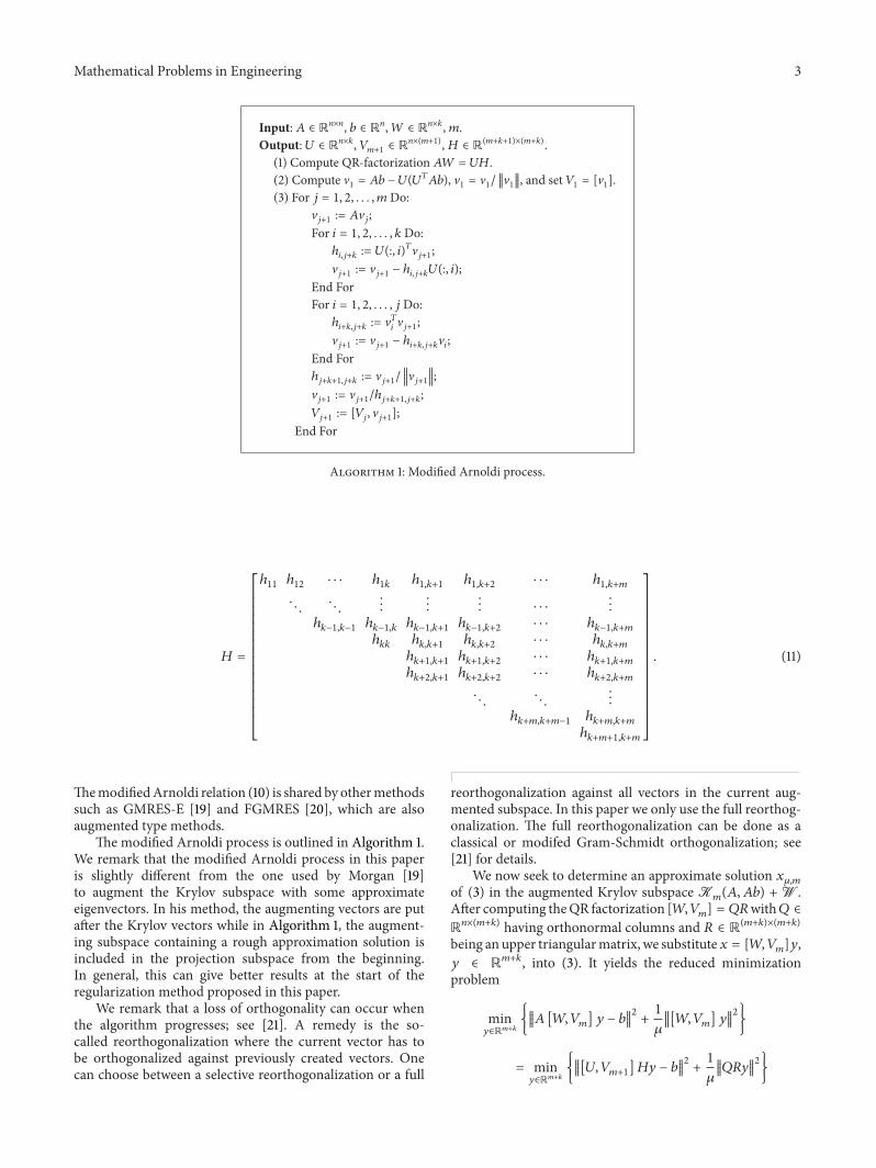
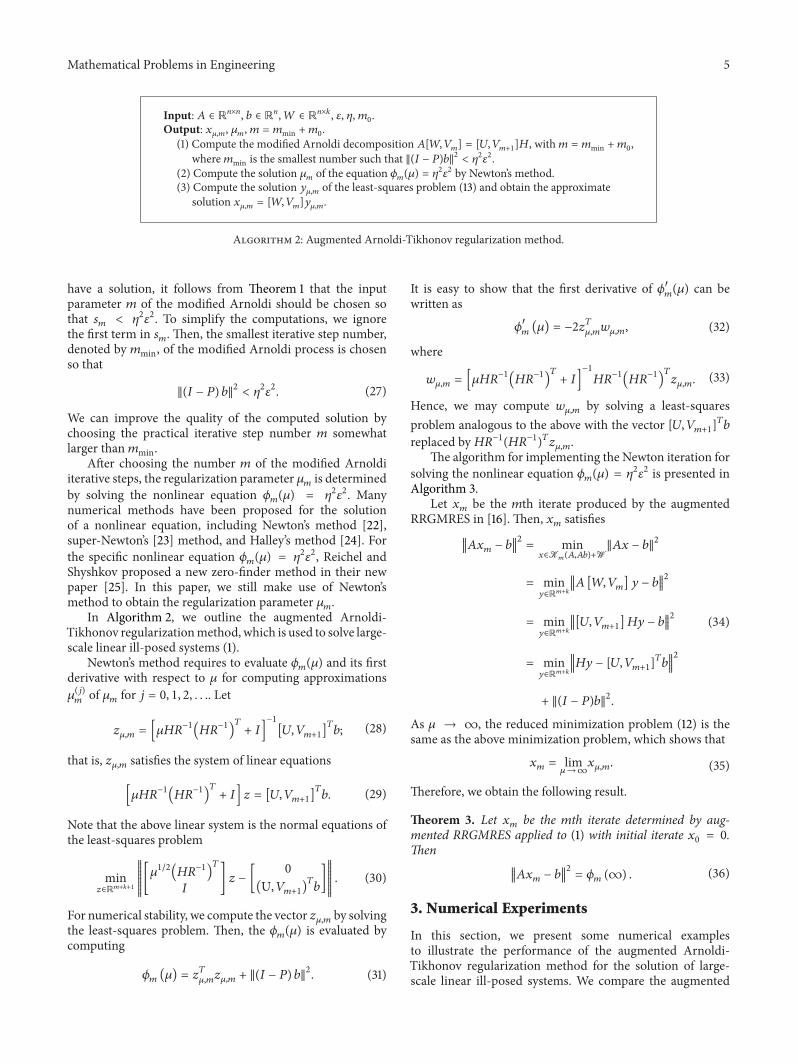


![CALIBRATION OF THE LOCAL VOLATILITY IN A GENERALIZED … · the general theory of Tikhonov regularization for ill-posed nonlinear inverse problems [21, 22, 27, 33, 34], both to the](https://img.pdfslide.net/doc/110x75/5edb0f4f09ac2c67fa68beae/calibration-of-the-local-volatility-in-a-generalized-the-general-theory-of-tikhonov.jpg)


![arXiv:2004.03941v1 [astro-ph.EP] 8 Apr 2020 › pdf › 2004.03941.pdf · two-year DSCOVR/EPIC observations presented byFan et al.(2019).The method with Tikhonov regularization enables](https://img.pdfslide.net/doc/110x75/5f04ce267e708231d40fcb86/arxiv200403941v1-astro-phep-8-apr-2020-a-pdf-a-200403941pdf-two-year.jpg)