1

Trade Booms, Trade Busts, and Trade Costs*

David S. Jacks (Simon Fraser University and NBER) Christopher M. Meissner (University of California, Davis and NBER)

Dennis Novy (University of Warwick)

August 2009

Abstract What has driven trade booms and trade busts in the past and present? We derive a micro-founded measure of trade frictions from leading trade theories and use it to gauge the importance of bilateral trade costs in determining international trade flows. We construct a new balanced sample of bilateral trade flows for 130 country pairs across the Americas, Asia, Europe, and Oceania for the period from 1870 to 2000 and demonstrate an overriding role for declining trade costs in the pre-World War I trade boom. In contrast, for the post-World War II trade boom we identify changes in output as the dominant force. Finally, the entirety of the interwar trade bust is explained by increases in trade costs. *We thank Alan M. Taylor for comments and Vicente Pinilla and Javier Silvestre for help with our data. We also appreciate the feedback from seminars at Calgary, Essex, Michigan, the New York Federal Reserve, Oxford, Stanford, Stockholm, UCLA, Valencia, and Zaragoza as well as from presentations at the 2008 Canadian Network for Economic History meetings, 2008 Western Economics Association meetings, the 2008 World Congress of Cliometrics meetings, and the 2009 Nottingham GEP Trade Costs Conference. Finally, Jacks gratefully acknowledges the Social Sciences and Humanities Research Council of Canada for research support. Novy gratefully acknowledges research support from the Economic and Social Research Council, grant RES-000-22-3112.

2

I. Introduction

Over the past two centuries, the world has witnessed two major trade booms and one

trade bust. Global trade increased at a remarkable pace in the decades prior to World War I as

well as in decades following World War II. In contrast, global trade came to a grinding halt

during the interwar period. What are the underlying driving forces of these trade booms and

busts? The goal of this paper is to address this question head-on by examining new data on

bilateral trade flows for a consistent set of 130 country pairs over the period from 1870 to 2000,

covering on average around 70 percent of global trade and output. We explore three eras of

globalization: the pre-World War I Belle Époque (1870-1913), the fractious interwar period

(1921-1939), and the post-World War II resurgence of global trade (1950-2000). Thus, the paper

is the first to offer a complete quantitative assessment of developments in global trade from 1870

all the way to 2000.1

Inevitably, any long-run view of international trade faces the notion that the structure of

economies changes over time. For example, international trade during the nineteenth century is

often viewed as being determined by relative resource endowments (Kevin H. O’Rourke and

Jeffrey G. Williamson, 1999) or differences in Ricardian comparative advantage (Peter Temin,

1997). More recently, international trade has been related to not only Ricardian factors (Jonathan

Eaton and Samuel S. Kortum, 2002) but also to the activities of heterogeneous firms (Marc J.

Melitz, 2003). The challenge for a long-run view is therefore to find a unifying framework that

accommodates a variety of divergent explanations for international trade. We invoke the gravity

equation to help us resolve this issue by exploiting the fact that gravity is consistent with a wide

1 We do, however, follow in the footsteps of other researchers that have looked at different periods in isolation. For instance, Antoni Estevadeordal, Brian Frantz, and Alan M. Taylor (2003) examine the period from 1870 to 1939. The work of Scott L. Baier and Jeffrey H. Bergstrand (2001) is the closest predecessor to our own. However, they only consider the period from 1958 to 1988. We also track changes in trade due to all trade costs while their data contained only rough proxies for freight costs and tariffs.

3

range of leading trade theories. While technical details might differ across models, all micro-

founded trade models produce a gravity equation of bilateral trade and all gravity equations have

in common that they relate bilateral trade to factors within particular countries such as economic

output and factors specific to country pairs such as bilateral trade costs. The intuition is that

gravity is simply an expenditure equation that arises in any general equilibrium trade model. It

describes how consumers allocate spending across countries—regardless of the motivation

behind international trade, be it international product differentiation or differences in

comparative advantage. In Section II below, we run standard gravity regressions and demonstrate

that gravity exerts its inexorable pull in all three sub-periods.

As a departure from previous work, we investigate the long-run evolution of trade costs.

These are all the costs of transaction and transport associated with the exchange of goods across

national borders. We define trade costs in a broad sense, including obvious barriers such as

tariffs and transport costs but also barriers that are more difficult to observe such as the costs of

overcoming language barriers and exchange rate risk. Even though trade costs are currently of

great interest (James E. Anderson and Eric van Wincoop, 2004; Maurice Obstfeld and Kenneth

S. Rogoff, 2000; David L. Hummels, 2007), little is known about the magnitude, determinants,

and consequences of trade costs.

Specifically, we derive a micro-founded measure of aggregate bilateral trade costs that is

consistent with leading theories of international trade. We are able to obtain this measure by

backing out the trade cost wedge that is implied by the gravity equation. This wedge gauges the

difference between observed trade flows and a hypothetical benchmark of frictionless trade. We,

therefore, infer trade costs from trade flows. This approach allows us to capture the combined

magnitude of tariffs, transport costs, and all other macroeconomic frictions that impede

4

international market integration but which are inherently difficult to observe. In Section III

below, we show that an isomorphic trade cost measure can be derived from a wide range of

leading trade theories—including the consumption-based trade model by Anderson and van

Wincoop (2003), the Ricardian model by Eaton and Kortum (2003), the heterogeneous firms

model by Thomas Chaney (2008) and the heterogeneous firms model with non-CES preferences

by Melitz and Gianmarco I.P. Ottaviano (2008). Intuitively, our approach exploits the fact that

all these models lead to a gravity equation in equilibrium. We emphasize that this approach of

inferring trade costs from readily available trade data holds clear advantages for applied

research: the constraints on enumerating—let alone, collecting data on—every individual trade

cost element even over short periods of time makes a direct accounting approach impossible.

In Section IV, we take the trade cost measure to the data. We find that in the forty years

prior to World War I, the average level of trade costs (expressed in tariff equivalent terms) fell

by thirty-three percent. From 1921 to the beginning of World War II, the average level of trade

costs increased by thirteen percent. Finally, average trade costs have fallen by sixteen percent in

the years from 1950. After describing the trends in trade costs, in Section V we examine whether

the trade cost measure is reliable. Our evidence suggests that standard trade cost proxies are

sensibly related to our measure. Factors like geographic proximity, adherence to fixed exchange

rate regimes, common languages, membership in a European empire, and shared borders all

matter for explaining trade costs. These factors alone account for roughly 30 to 50 percent of the

variation in trade costs. However, the three sub-periods exhibit significant differences, allowing

us to document important changes in the global economy over time such as the growing

importance of distance in determining the level of trade costs and the diminishing effects of fixed

exchange rate regimes and membership in European empires on trade costs over time.

5

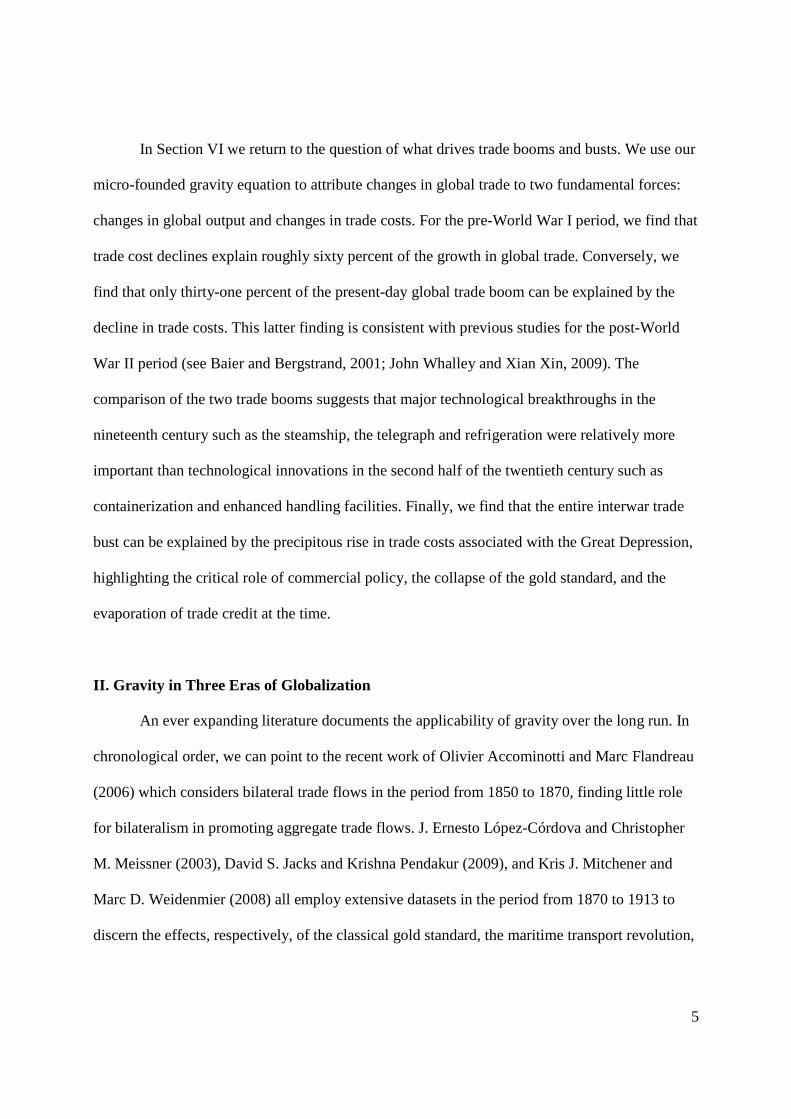
In Section VI we return to the question of what drives trade booms and busts. We use our

micro-founded gravity equation to attribute changes in global trade to two fundamental forces:

changes in global output and changes in trade costs. For the pre-World War I period, we find that

trade cost declines explain roughly sixty percent of the growth in global trade. Conversely, we

find that only thirty-one percent of the present-day global trade boom can be explained by the

decline in trade costs. This latter finding is consistent with previous studies for the post-World

War II period (see Baier and Bergstrand, 2001; John Whalley and Xian Xin, 2009). The

comparison of the two trade booms suggests that major technological breakthroughs in the

nineteenth century such as the steamship, the telegraph and refrigeration were relatively more

important than technological innovations in the second half of the twentieth century such as

containerization and enhanced handling facilities. Finally, we find that the entire interwar trade

bust can be explained by the precipitous rise in trade costs associated with the Great Depression,

highlighting the critical role of commercial policy, the collapse of the gold standard, and the

evaporation of trade credit at the time.

II. Gravity in Three Eras of Globalization

An ever expanding literature documents the applicability of gravity over the long run. In

chronological order, we can point to the recent work of Olivier Accominotti and Marc Flandreau

(2006) which considers bilateral trade flows in the period from 1850 to 1870, finding little role

for bilateralism in promoting aggregate trade flows. J. Ernesto López-Córdova and Christopher

M. Meissner (2003), David S. Jacks and Krishna Pendakur (2009), and Kris J. Mitchener and

Marc D. Weidenmier (2008) all employ extensive datasets in the period from 1870 to 1913 to

discern the effects, respectively, of the classical gold standard, the maritime transport revolution,

6

and the spread of European overseas empires on bilateral trade flows. For the interwar period,

Barry J. Eichengreen and Doug A. Irwin (1995) are able to document the formation of currency

and trade blocs by using an early variant of gravity, while Estevadeordal, Frantz and Taylor

(2003) trace the rise and fall of world trade over the longer period from 1870 to 1939, offering a

revisionist history where the collapse of the resurrected gold standard and the increase in

maritime freight costs all play a role in explaining the interwar trade bust. Finally, for the post-

World War II period, a non-exhaustive list of nearly 100 gravity oriented papers is cataloged by

Anne-Celia Disdier and Keith Head (2008).

It is clear that the validity of the gravity model of international trade has been firmly

established theoretically and empirically, both now and in the past. But what has been lacking is

a unified attempt to exploit gravity to explain the three eras of globalization. In what follows, we

present the results of just such an attempt. A typical estimating equation for a gravity model of

trade often takes the form of:

(1) ln( ) ln( ) ,ijt it jt it jt ijt ijtx y y zα α γ β ε= + + + +

where xijt represents bilateral exports from country i to j in time t; the αit and αjt terms represent

importer and exporter country fixed effects intended to capture differences in relative resource

endowments, differences in productivity, and any other time-invariant country attributes which

might determine a country’s propensity for export or import activity; the yit and yjt terms

represent gross domestic products in countries i and j; and zijt is a row vector of variables

representing the various bilateral frictions that limit the flow of goods between countries i and j

and includes familiar standbys in the literature such as the physical distance separating countries.

We use expression (1) along with the trade and output data detailed in Appendix I to

chart the course of gravity in three eras of globalization: the pre-World War I Belle Époque

7

(1870-1913), the fractious interwar period (1921-1939), and the post-World War II resurgence of

global trade (1950-2000). The 27 countries in our sample include Argentina, Australia, Austria,

Belgium, Brazil, Canada, Denmark, France, Germany, Greece, India, Indonesia, Italy, Japan,

Mexico, the Netherlands, New Zealand, Norway, the Philippines, Portugal, Spain, Sri Lanka,

Sweden, Switzerland, the United Kingdom, the United States, and Uruguay. Figure 1

summarizes the sample graphically.2 Finally, we incorporate measures for distance, the

establishment of fixed exchange rate regimes, the existence of a common language, historical

membership in a European overseas empire,3 and the existence of a shared border.4 Summary

statistics and the results of this exercise of estimating gravity in the three sub-periods separately

are reported in Tables 1 and 2, respectively.

In Panel A of Table 2, we estimate equation (1) by OLS, using GDP, the five variables

proxying for trade costs mentioned above, and country fixed effects. The results are reassuring.

The coefficients on GDP—although different across the three eras of globalization—are

precisely estimated and fall within the bounds established by previous researchers. Likewise,

distance is found to be negatively and significantly related to bilateral trade flows. Fixed

exchange rate regimes, common languages, and shared borders are all found to be positively and

significantly associated with bilateral trade flows. We also note that these regressions confirm

the emerging story on the pro-trade effects of empires, specifically the very strong stimulus to

2 This sample constitutes, on average, 72% of world exports and 68% of world GDP over the entire period. We also note that the various sub-samples are highly balanced. Given the 130 country pairs in our sample, there are 14,820 possible bilateral trade observations (130 times 114 years) of which we are able to capture fully 99.9%. 3 For all intents and purposes, this may be thought of as an indicator variable for the British Empire. The sole exception in our sample is the case of Indonesia and the Netherlands. 4 Another obvious candidate is commercial policy, and especially tariffs. Only one consistent measure of tariffs is available for the period from 1870 to 2000 in the form of the customs duties to declared imports ratio as in Michael A. Clemens and Williamson (2001). This measure seems to be a reasonably good proxy for tariffs in the pre-World War I and interwar periods. However, after 1950 and the well-known rise of non-tariff barriers to trade, this measure becomes unreliable, sometimes registering unbelievably low levels of protection. The measure also—somewhat paradoxically—becomes less readily available after World War II; the United Kingdom, for instance, stops reporting the level of customs duties in 1965.

8

trade afforded by European empires in the pre-World War I period (Mitchener and Weidenmier,

2008) which slowly faded in light of the disruptions of the interwar period and the

decolonization movement of the 1950s and 1960s (Head, Thierry Mayer, and John Ries, 2008).

In addition, this simple specification explains a remarkably high percentage of the variation in

bilateral trade flows for each of the separate periods as the adjusted R-squared ranges from a low

of 0.64 in the Belle Époque period to a high of 0.84 in the period from 1950 to 2000.

A more exacting specification consistent with the recent gravity literature (Anderson and

van Wincoop, 2003 and Richard E. Baldwin and Daria Taglioni, 2007) would be that in Panel B.

Along with the proxies for trade costs, this specification includes year fixed effects, and allows

the country fixed effects to change over time. Thus, for the period from 1870 to 1913, there are

44 years and 27 countries, yielding 1188 country-specific annual fixed effects. Likewise, there

are 513 (=19*27) country-specific annual fixed effects for the period from 1921 to 1939 and

1377 (=51*27) country-specific annual fixed effects for the period from 1950 to 2000. In

addition, we drop the GDP term in light of its perfect collinearity with the annual fixed effects.

The sign and significance of the remaining variables is remarkably consistent across the panels.

To conclude, the fundamental result of this section has been that gravity exerts its pull, no

matter the period and no matter what the underlying drivers of trade—be they relative resource

endowments, differences in productivity, or product differentiation across countries. We seem to

be on firm ground when asserting the consistency of gravity in determining international trade

flows, both in the past and the present. This is a key result which we argue motivates the use of a

common gravity model of trade for the three eras of globalization. We develop such a model in

the following section.

9

III. Gravity Redux

As we demonstrate above, the standard gravity equation (1) holds up well in predicting

trade flows over different periods. As a first step, we point out that a gravity equation similar to

equation (1) can be derived from a wide range of leading trade models: (i) the Anderson and van

Wincoop (2003) trade model that focuses on multilateral resistance, (ii) the Ricardian trade

model by Eaton and Kortum (2002), (iii) the trade model with heterogeneous firms by Chaney

(2008), based on Melitz (2003), and (iv) the heterogeneous firms model by Melitz and Ottaviano

(2008) with a linear, non-CES demand structure. This confirms the appeal of the gravity

equation: although the driving forces behind international trade differ across these models—say,

Ricardian comparative advantage versus love of variety—they all predict a gravity equation as

an equilibrium for international expenditure patterns.5

In a second step, we exploit the fact that these trade models predict the same gravity

structure. In particular, we formally show that all the gravity equations can be solved for the

implied trade cost expression used below.6 These implied trade costs can be interpreted as the

wedge between a hypothetical frictionless world as predicted by each model and the actual trade

patterns observed in the data. We argue that these implied trade costs are an informative

summary statistic to describe international trade frictions. In a later section, we also demonstrate

this empirically.

5 Gene M. Grossman (1998, p. 29-30) neatly summarizes this situation: “Specialization lies behind the explanatory power [of the gravity equation], and of course some degree of specialization is at the heart of any model of trade…This is true no matter what supply-side considerations give rise to specialization, be they increasing returns to scale in a world of differentiated products, technology differences in a world of Ricardian trade, large factor endowment differences in a world of Heckscher-Ohlin trade, or (small) transport costs in a world of any type of endowment-based trade.” [Emphasis in original] 6 Also see Dennis Novy (2009).

10

(i) Gravity in Anderson and van Wincoop (2003)

Anderson and van Wincoop (2003) derive the following gravity equation:

1

(2) ,i j ijij W

i j

y y tx

y P

σ−

= Π

where Wy is world output and iΠ and jP are outward and inward ‘multilateral resistance’

variables. The latter can be interpreted as average trade barriers. 1≥ijt is the bilateral trade cost

factor (one plus the tariff equivalent), and 1>σ is the elasticity of substitution. In empirical

applications, trade costs are typically proxied by variables such as bilateral distance and a border

dummy. But it is difficult to find empirical proxies for the multilateral resistance variables.

Anderson and van Wincoop (2003) caution against the use of price indices since they might not

capture non-pecuniary trade barriers. Instead, the procedure that has been adopted most

frequently in recent gravity applications is to include country fixed effects.

As an alternative, we follow Novy (2009) in eliminating the multilateral resistance

variables from the gravity equation. The counterpart of equation (2) for domestic tradeiix is

1

(3) .i i iiii W

i i

y y tx

y P

σ−

= Π

When equation (2) is multiplied by its counterpart for bilateral trade from j to i, jix , we obtain

the product of all multilateral resistance variables on the right-hand side, jiji PPΠΠ . These

multilateral resistance indices can be eliminated by dividing by the product of domestic trade

flows, jjii xx :

1

(4) .ij ji ij ji

ii jj ii jj

x x t t

x x t t

σ−

=

11

We solve for the trade costs as the key parameters of interest. The parentheses on the right-hand

side of equation (4) contain the product of two trade cost ratios. These ratios represent the extent

to which bilateral trade costs ijt and jit exceed domestic trade costs iit and jjt . Finally, we take

the square root to form their geometric average and subtract by one to get an expression for the

tariff equivalent. The resulting expression is

( )1 1

2 2 1

(5) 1 1,ij ji ii jjij

ii jj ij ji

t t x x

t t x x

σ

τ−

≡ − = −

where ijτ is the trade cost wedge that captures bilateral relative to domestic trade costs.

To grasp the intuition behind this trade cost measure, imagine the two extremes of a

frictionless world and a closed economy. In a frictionless world, all trade cost factors ijt , jit , iit

and jjt are equal to 1. It follows that 0=ijτ . In contrast, a closed economy is characterized by

bilateral trade flows, jiij xx , that are zero. In that case, ijτ approaches infinity. ijτ can therefore

be interpreted as a trade cost wedge that measures just how far bilateral trade integration is away

from a hypothetical frictionless world. Note that this trade cost measure does not impose bilateral

trade cost symmetry. Bilateral trade costs, ijt and jit , may differ under this framework but here,

we can only identify their geometric average but not the extent to which they diverge. In

addition, we do not impose zero domestic trade costs. Finally, we note that non-unitary income

elasticities, as found by João M.C. Santos Silva and Silvana Tenreyro (2006), do not pose a

problem for our methodology. It is easy to show that if the income elasticity in gravity equation

(2) differed from unity, the trade cost measure in equation (5) would not be affected.

We have derived the trade cost measure in equation (5) from the well-known Anderson

and van Wincoop (2003) gravity model. An Armington assumption is imposed in their model so

12

that countries are endowed with differentiated goods, and trade is driven by consumers’ love of

variety. To show that our trade cost measure ijτ is not dependent on one specific trade model, we

now derive this measure from other leading trade models.

(ii) Gravity in Eaton and Kortum (2002)

In the Ricardian model by Eaton and Kortum (2002), productivity in each country is

drawn from a Fréchet distribution that has two parameters, iT and ζ . iT determines the location

of the productivity distribution for country i, with a high iT denoting high overall productivity.

1>ζ denotes the variation within the distribution and is treated as common across countries,

with a high ζ denoting little variation. The model yields a gravity equation for an aggregate of

homogeneous goods whose structure is related to equation (2). It is given by

( )( )

(6) ,i i ijij

j i i iji

T c tx

x T c t

ζ

ζ

−

−=∑

where jx denotes country j’s total expenditure and ic denotes the input cost in country i.

As in the context of the Anderson and van Wincoop (2003) model, we are interested in

the trade cost parameters. iT and ic are unobservable but cancel out once the ratio of domestic

over bilateral trade flows is formed as in equation (5). This yields

1 1

2 2

(7) 1 1.ij ji ii jjEKij

ii jj ij ji

t t x x

t t x x

ζ

τ

= − = −

Comparing equations (5) and (7), it is obvious that ijEKij ττ = if 1−= σζ .7

7 For more details on the comparison of Armington-type and Ricardian models, see Eaton and Kortum (2002, footnote 20) and Anderson and van Wincoop (2004, pp. 709-710).

13

(iii) Gravity in Chaney (2008)

Chaney (2008) builds on the seminal paper by Melitz (2003) and derives a gravity

equation based on a model with heterogeneous productivities across firms and fixed costs of

exporting. In contrast to previous trade models, the two assumptions of heterogeneous firms and

fixed costs of exporting introduce an extensive margin of trade. Not only do exporters vary the

size of shipments (the intensive margin) in response to changes in trade costs, but also the set of

exporters changes (the extensive margin). Chaney derives the following industry-level gravity

equation

( ) 11(8) ,i j i ij

ij ijWj

y y w tx f

y

γγ

σ

λ

− − − −

=

where iw is workers’ productivity in country i, jλ is a remoteness variable akin to multilateral

resistance, and ijf are the fixed costs of exporting from country i to j.8 γ is the shape parameter

of the Pareto distribution from which productivities are drawn, with a high γ denoting a low

degree of heterogeneity and 1−> σγ . Forming the ratio of domestic over bilateral trade flows

yields

1 1 1 1 1

2 2 1 2

(9) 1 1.ij ji ij ji ii jjChij

ii jj ii jj ij ji

t t f f x x

t t f f x x

σ γ γ

τ

− − = − = −

Chijτ is a now function of both variable and fixed trade costs. Thus, under the assumptions of

Chaney’s (2008) model the interpretation of the trade cost wedge extends to fixed costs of

exporting.

8 The economy is modeled as one industry.

14

We note that for non-zero trade flows (as is generally the case in our sample), the

heterogeneous firms model by Elhanan Helpman, Marc J. Melitz, and Yona Rubinstein (2008) is

consistent with the same trade cost measure as in equation (9), that is, Chij

HMRij ττ = .9

(iv) Gravity in Melitz and Ottaviano (2008)

Melitz and Ottaviano (2008) also model heterogeneous firms. Firms face sunk costs of

market entry, Ef , that can be interpreted as product development and production start-up costs.

In contrast to Melitz (2003) and Chaney (2008), exporting firms only face variable trade costs

and no fixed costs of exporting. The model is based on non-CES preferences that give rise to

endogenous markups. More specifically, markups tend to be low in large markets with many

competitors.

The multiple-country version of their model leads to the following gravity equation:

( ) ( ) ( )21(10) ,

2 2i i j j

ij E d ijx N L c tγ γ

ψδ γ

+ −=

+

where δ is a parameter from the utility function that indicates the degree of product

differentiation, with a higher δ meaning a higher degree of differentiation. iEN is the number of

entrants in country i. An index of comparative advantage in technology is given by iψ with a

high value meaning that entrants in country i have a high chance of obtaining favorable

productivity draws. jL denotes the number of consumers in country j, and jdc is the marginal

cost cut-off above which domestic firms in country j do not produce. The intuition is that tougher

9 In the notation of Helpman, Melitz and Rubinstein (2008), non-zero trade flows imply Vij>0∀ i,j . To obtain

Chij

HMRij ττ = we also assume positive fixed costs for domestic sale, fii>0. We also need to allow for positive

domestic variable trade costs, tii≥1∀ i, and, as in Appendix II of their paper, assume there is no upper bound in the support of the productivity distribution, aL=0.

15

competition in country j, reflected by a lower jdc , makes it harder for exporters from i to break

into that market. Forming the ratio of domestic over bilateral trade flows yields

1 1

2 2

(11) 1 1.ij ji ii jjMOij

ii jj ij ji

t t x x

t t x x

γ

τ

= − = −

In contrast to Chijτ in equation (9), neither sunk nor fixed costs enter MO

ijτ because all firms face

identical entry costs, Ef , and no fixed costs of exporting. Variable trade costs are sufficient to

induce selection into export markets because of bounded non-CES marginal utility

(v) Gravity in Deardorff (1998)

Finally, Alan V. Deardorff (1998) argues that in a Heckscher-Ohlin world with bilateral

trade barriers, a model similar to the one by Anderson and van Wincoop (2003) applies. The

intuition is that bilateral trade barriers prevent factor price equalization between two countries

that trade with each other. If factor prices were equalized, final goods prices would also be

equalized and neither country could overcome the trade barriers. In a world with a large number

of goods and few factors it is, therefore, likely that one country will be the lowest-cost producer.

Trade in a Heckscher-Ohlin world would, thus, resemble trade in an Armington world and could

be characterized by a standard gravity equation.

In summary, the reason why our trade integration measure ijτ is consistent with a broad

range of trade models is related to the fact that they all lead to gravity equations that have a

similar structure as equation (2). In a similar vein, Robert C. Feenstra, James R. Markusen, and

Andrew K. Rose (2001) and Simon J. Evenett and Wolfgang Keller (2002) also show that

gravity equations are consistent with various competing trade models. Intuitively, the gravity

equation simply indicates how consumers allocate their expenditure across countries subject to

16

trade frictions (Baldwin and Taglioni, 2007). Gravity equations arise regardless of why

consumers want to buy goods from foreign countries. In an Armington world, consumers buy

foreign goods because those goods are inherently different and consumers prefer variety. In a

Ricardian world, countries produce goods according to comparative advantage and consumers

buy foreign goods because they are cheaper. It turns out that the particular motivation behind

foreign trade is not crucial to understand the role of bilateral trade frictions.

IV. Trade Costs over Time

We use equation (5) along with the trade and output data detailed in Appendix I to

construct bilateral trade costs for the 130 country pairs in our sample. Lacking consistent data on

domestic trade, we use GDP less aggregate exports instead. However, a potential problem arises:

the GDP data are value-added whereas trade data typically reported as gross values. For the post-

World War II period, it becomes possible to track how well this proxy performs by comparing it

to domestic trade constructed as total manufacturing production less total exports. The results are

favorable in that although the level of bilateral trade costs is affected by the way domestic trade

is measured, the change over time is remarkably similar (Novy, 2009). For example, in the case

of U.S.-Canadian trade costs over the period from 1970 to 2000, the correlation between the

measure based on GDP data and the one based on production data is 0.96. 10

The elasticity of substitution, σ, typically falls in the range (5,10) as surveyed by

Anderson and van Wincoop (2004). As (σ-1) in equation (6) corresponds to the Fréchet

parameter ζ in equation (8) and the Pareto parameter γ in equations (11) and (14), it is instructive

to also consider estimates for those parameters. Eaton and Kortum (2002) report a baseline

10 The intuition for the high correlation is that the increase in the (gross) production data is approximately matched by the increase in the (value-added) GDP data because the latter includes the growth of the services sector. See Novy (2009).

17

estimate of 8.3 for ζ. Chaney (2008) estimates the ratio γ/(σ-1) to be near two, which suggests a

value of γ above σ. We set the value of σ to eight, which roughly corresponds to the midpoint of

the range (5,10). But we show in Appendix III that although the level of inferred trade costs is

sensitive to the assumed parameter value, the change of trade costs over time is hardly affected.

Average trade cost series are generated for each of the three eras of globalization by

regressing the constructed bilateral trade costs on a set of year fixed effects. This exercise is

replicated for both global trade and six sub-regions: within the Americas, within Asia/Oceania,

within Europe, between the Americas and Asia/Oceania, between the Americas and Europe, and

between Asia/Oceania and Europe. Figures 2 through 4 track these averages over time. There,

the averages have all been normalized to 100 for the initial observation in each period, i.e. 1870,

1921, and 1950, so that they are not strictly comparable in terms of levels across periods. Our

goal instead is to highlight the changes within a given period. We are also trying to avoid

pressing too hard on the assumption that the substitution elasticity (or alternatively, the Fréchet

or Pareto parameters) have remained constant over the entire 130 years under consideration.11

We weight these averages by GDP to reduce the influence of country pairs which trade

infrequently or inconsistently.12

Thus, for the first wave of globalization from 1870 to 1913, we document an average

decline in international trade costs relative to domestic trade costs of thirty-three percent.13 This

was led by a fifty percent decline for trade between Asia/Oceania and Europe, probably

generated from a combination of Japanese reforms that increased engagement with the rest of the

11 See Appendix III for a robustness check. 12 The obvious candidate for weights, the level of bilateral trade, is inappropriate in this instance. A quick look at equation (5) verifies that bilateral trade and trade costs are not independent. That is, a low trade cost measure is generated for a country pair with high bilateral trade, suggesting that the use of bilateral trade would impart systematic downward bias in the weighted average. 13 The distribution of spikes in 1874 and 1881 in the Asia and Americas-Asia series may seem odd. However, these are explained by the small number of underlying observations (n=7 and n=6, respectively) and can be attributed to sporadic trade volumes for Japan as it integrated—sometimes by fits and starts—into the global economy.

18

world, the consolidation of European overseas empires, and radical improvements in

communication and transportation technologies which linked Eurasia. These gains were

apparently not limited to the linkages between the countries of Asia/Oceania and the rest of the

world as intra-Asian/Oceanic trade costs declined on the order of thirty-seven percent. Thus, the

late nineteenth century was a time of unprecedented changes in the relative commodity and

factor prices of the region as has been documented by Jeffrey G. Williamson (2006).

Bringing up the rear was intra-American trade, albeit with a still respectable average

decline of nineteen percent. This performance masks significant heterogeneity across North and

South America: trade costs within North America declined twenty-nine percent, while trade costs

between North and South America fell by only fifteen percent. Most likely, this reflects South

America’s continued orientation towards European markets and the fleeting connections uniting

South America and North America—save the United States—at the time. Likewise, intra-

European trade costs only declined twenty-one percent. This performance reflects the maturity as

well as the proximity of these markets. We should also note that a substantial portion of the

decline is concentrated in the 1870s. This was, of course, a time of simultaneously declining

freight rates and tariffs as well as increasing adherence to the gold standard. In subsequent

periods, the decline in freight rates was substantially moderated, while tariffs climbed in most

countries, dating from the beginning of German protectionist policy in 1879.

Turning to the interwar period from 1921 to 1939, we can see that the various attempts to

restore the pre-war international order were somewhat successful at reining in international trade

costs. A fitful return to the gold standard was launched in 1925 when the United Kingdom

returned to gold convertibility at the pre-war parity. By 1928, most countries had followed its

lead and stabilized their currencies. At the same time, the international community witnessed a

19

number of attempts to normalize trading relations, primarily through the dismantling of the

quantitative restrictions erected in the wake of World War I (Ronald Findlay and Kevin H.

O’Rourke, 2007). As a result, trade costs fell on average by seven percent up to 1929. Although

much less dramatic than the fall for the entire period from 1870 to 1913, this average decline was

actually twice as large as that for the equivalent period from 1905 to 1913, pointing to a

surprising resilience in the global economy of the time. The leaders in this process were again

trade between Asia/Oceania and Europe with a respectable fifteen percent decline and intra-

European trade with a ten percent decline. On the other end of the spectrum, trade costs within

the Americas and between the Americas and Europe barely budged, both registering a three

percent decline. And again, these aggregate figures for the Americas mask important differences

across North and South America: trade costs within North America ballooned by eight percent—

reflecting the adversarial commercial policy of Canada and the United States in the 1920s—

while trade costs between North and South America declined by seven percent.

The Great Depression marks an obvious turning point for all the series. It generated the

most dramatic increase in average trade costs in our sample as they jump by twenty-one

percentage points in the space of the three years between 1929 and 1932. This, of course, exactly

corresponds with the well-documented implosion of international trade in the face of declining

global output (Angus Maddison, 2003), highly protectionist trade policy (Jakob B. Madsen,

2001), tight commercial credit (William Hynes, David S. Jacks, and Kevin H. O’Rourke, 2009),

and a generally uneasy trading environment. Trade costs within Asia/Oceania, within Europe,

and between Asia/Oceania and Europe experienced the most moderate increases at eighteen

percentage points each. Trade costs within the Americas rose very strongly by thirty-five

percentage points, driven more by the trade disruptions between North and South America (+38

20

percentage points) than within North America (+28 percentage points). Over time though, trade

costs declined from these heights just as the Depression slowly eased from 1933 and nations

made halting attempts to liberalize trade, even if only on a bilateral or regional basis (Findlay

and O’Rourke, 2007). Yet these were not enough to recover the lost ground: average trade costs

stood thirteen percent higher at the outbreak of World War II than in 1921.

Finally, the second wave of globalization from 1950 to 2000 registered declines in

average trade costs on the order of sixteen percent. The most dramatic decline was that for intra-

European trade costs at thirty-seven percent, a decline that is surely related to the formation of

the European Economic Community and subsequently the European Union. The most

recalcitrant performance was that for the Americas and Asia/Oceania, both of which registered

small increases in bilateral relative to domestic trade costs over this period. In the former case,

this curious result is solely generated by trade costs between North and South America which

rose by twenty-two percent. This most likely reflects Argentina, Brazil, and Uruguay’s

adherence to import-substituting industrialization up to the debt crisis of the 1980s and the

reorientation of South American trade away from its heavy reliance on the United States as a

trading partner which had emerged in the interwar period. In contrast, trade costs within North

America fell by a remarkable sixty percent, at least partly reflecting the formation of the North

American Free Trade Agreement and its forerunners. In the case of Asia/Oceania, the rise in

trade costs is primarily generated by India which in its post-independence period simultaneously

erected formidable barriers to imports and retreated from participation in world export markets.

Curiously, this India effect is most pronounced for former fellow members in the British Empire,

that is, Australia, New Zealand, and Sri Lanka.

21

Most surprisingly, the decline in international relative to domestic trade costs in the

second wave of globalization is mainly concentrated in the period before the late 1970s. Indeed,

in the global and all sub-regional averages—save the Americas—trade costs were lower in 1980

than in 2000. In explaining the dramatic declines prior to 1973, one could point to the various

rounds of the GATT up to the ambitious Kennedy Round which concluded in 1967 and slashed

tariff rates by 50% and which more than doubled the number of participating nations. Or

perhaps, it could be located in the substantial drops—but subsequent flatlining—in both air and

maritime transport charges up to the first oil shock documented in Hummels (2007). This curious

phenomenon demands further attention but remains outside the scope of this paper.

V. The Determinants of Trade Costs

Having traced the course of trade costs, we now consider some of their likely

determinants. This exercise serves two purposes. First, it addresses—albeit imperfectly—the

natural question of what factors have been driving the evolution of trade costs over time. Second

and more importantly, it helps further establish the reliability of our measure of trade costs—that

is, are trade costs as constructed in this paper reasonably correlated with other variables

commonly used as proxies in the literature? Below, we demonstrate that this is the case. We also

refer the reader to Appendix II where we provide two additional robustness checks.

Trade costs in our model are derived from a gravity equation rather than estimated as is

typically the case in the literature. Commonly, log-linear versions of equation (1) are estimated

by substituting an arbitrary trade cost function for zijt and using country-pair fixed effects for the

multilateral resistance variables. Such gravity specifications, to the extent that the trade cost

function and the econometric model are well specified, could be used to provide estimated values

22

of trade costs. In fact, such specifications have been highly successful in explaining a significant

proportion of the variance in bilateral trade flows as demonstrated above. Nevertheless, there is

likely a substantial amount of unexplained variation due to unobservable trade costs and, thus,

potential omitted variable bias.

Consider the standard function for trade costs that the vast majority of the gravity

literature imposes

(12) dist exp( ),ijt ij ijt ijtxρ

τ α β ε= +

where dist is a measure of distance between two countries, x is a row vector of observable

determinants of trade costs, and ε is an error term composed of unobservables. We log-linearize

(12). The determinants we consider are the same as those in Section II and include the distance

between two countries, the establishment of fixed exchange rate regimes, the existence of a

common language, membership in a European overseas empire, and the existence of a shared

border. In all regressions, we include time-invariant exporter and importer fixed effects as well

as year fixed effects.14 The reported regressions pool across all periods and then separate the data

for the 130 dyads between 1870 and 1913, 1921 and 1939, and 1950 and 2000. The results are

reported in Table 3.

Considering the pooled results first, we find that a one standard deviation rise in distance

raises trade costs by 0.38 standard deviations. Fixed exchange rates, a common language, joint

membership in a European empire, and sharing a border all decrease trade costs with the latter

two coefficients being roughly double the estimated effect of fixed exchange rate or sharing a

common language. This pooled approach demonstrates that standard factors that are known to be

frictions in international trade are sensibly related to the trade cost measure. The results also

14 By construction τij nets out the multilateral resistance terms so that time-varying importer and exporter fixed effects are not required.

23

show that the trade cost measure determines trade patterns in ways largely consistent with the

gravity literature covering more geographically comprehensive samples.

At the same time, the pooled approach masks significant heterogeneity across the periods.

Here, we would like to highlight a few of these differences. First, fixed exchange rate regimes

appear noticeably stronger in the pre-World War I and post-World War II environments—a

result consistent with the tenuous resurrection of the classical gold standard in the interwar

period (Natalia Chernyshoff, Jacks, and Taylor, 2009). Second, a common language seems to

have exerted a slightly stronger force (roughly 75%) on trade costs in the period from 1870 to

1913 than subsequently. Third, we are able to document a strongly diminished role for European

empires in reducing trade costs: a coefficient of -0.46 from 1870 to 1913 is reduced to -0.15 in

the period from 1950 to 2000—a result which is again consistent with the recent work of Head,

Mayer, and Ries (2008).15 Finally, distance seems to have become more important in the post-

1950 world economy, with the coefficient increasing by 50 percent as compared to 1870-1913 or

almost tripling when compared to 1921-1939. This result is in line with Disdier and Head (2008)

who find that the estimated distance coefficient has been on the rise from 1950 in their meta-

analysis of the gravity literature. Whether this reflects upward pressures in transport costs

(Hummels, 2007), the regionalization of trade or changes in the composition of traded goods

remains an open question, but it does accord with the empirical evidence on the decreasing

distance-of-trade from the 1950s (Matias Berthelon and Caroline Freund, 2008; Celine Carrère

and Maurice Schiff, 2005).

One way to get a sense of the relative contribution of the five variables to the variation in

trade costs is to compare the R-squareds from a battery of regressions as in the work of Kalina

15 Interestingly, much of this decline had already happened prior to 1950 as the coefficient registers a value of -0.20 during the interwar period.

24

Manova (2008). Specifically, one can generate an upper bound for the contribution of, say,

distance by re-estimating (12) with only that variable but no other controls. Thus, the upper

bound loads as much variation as possible onto distance. One can also generate a lower bound

for the contribution of distance by using the difference between the R-squareds from the fixed

effects specification with all variables of interest including distance—as in the corresponding

panel of Table 3—and a fixed effects specification with all variables of interest excluding

distance. Thus, the lower bound represents the marginal contribution of distance to an otherwise

full specification.

In Table 4, we report the results of running such regressions and tabulating the R-

squareds for each variable in each sub-period. Thus, we find that distance can explain between 2

and 14 percent of the variation in trade costs in the period from 1870 to 1913. What is apparent

from Table 4 is that the relative contribution of the five variables remains highly consistent

across the three sub-periods, with distance potentially explaining the most variation and

historical membership in European overseas empires the least variation. The results in Table 4

also confirm the increasing explanatory power of distance over time—and especially in the post-

1950 period—and the decreasing explanatory power of fixed exchange rate regimes and the

historical membership in European overseas empires hinted at above.

VI. Changes in Output versus Changes in Trade Costs

In order to determine what drives trade booms and busts, we now turn to a decomposition

of the growth of trade flows in the three periods. We are interested in whether trade booms are

mainly related to secular increases in output or falling trade costs. Similarly, we are interested in

whether trade busts are mainly related to output slumps or increasing trade costs. Our gravity

25

framework easily lends itself to answering these questions. Below, we outline our approach

based on the Anderson and van Wincoop (2003) gravity model but we note that identical results

can be obtained based on the models by Eaton and Kortum (2002), Chaney (2008), and Melitz

and Ottaviano (2008).

We rewrite equation (4) as

( ) ( )1

2 1(13) 1 .ij ji ii jj ii jj

ij ji i j i j ijii jj i j i j

t t x x x xx x y y y y

t t y y y y

οο

τ−

− = = +

As we are interested in the growth of bilateral trade, we log-linearize equation (13) and take the

first difference between years (denoted by ∆). This yields

( ) ( ) ( ) ( )(14) ln ln 2 1 ln 1 ln ii jjij ji i j ij

i j

x xx x y y

y yσ τ

∆ = ∆ + − ∆ + + ∆

Following Helpman (1987) and Baier and Bergstrand (2001), we split the product of outputs into

the sum of outputs and output shares, ( ) jijiji ssyyyy 2+= with ( )jiii yyys += / , such that we

obtain our final decomposition,

( ) ( ) ( ) ( ) ( )(15) ln 2 ln ln 2 1 ln 1 ln ii jjij ji i j i j ij

i j

x xx x y y s s

y yσ τ

∆ = ∆ + + ∆ + − ∆ + + ∆

Equation (15) decomposes the growth of bilateral trade into four components. The first term on

the right-hand side represents the contribution of output growth to bilateral trade growth. The

second term is the contribution of increasing income similarity, as first stated by Helpman

(1987). All else being equal, two countries of the same size are expected to generate more

international trade than two countries of unequal size. The third term reflects the contribution of

changes in trade costs as measured by τij.16 The fourth term represents changes in multilateral

16 Since (1-σ) is negative, a decline in τij implies a positive third term on the right-hand side of equation (19).

26

factors. Its precise interpretation depends on the underlying trade model. For example, as

equation (3) shows, if multilateral trade barriers fall over time, the ratio of domestic trade to

output iii yx / goes down so that the contribution of the fourth term to bilateral trade growth

becomes negative. This can be interpreted as a trade diversion effect that is consistent with the

models by Anderson and van Wincoop (2003), Eaton and Kortum (2002), and Chaney (2008).17

We consider the growth of bilateral trade between the initial years (1870, 1921 and 1950)

and the end years (1913, 1939 and 2000) of our three sub-periods. We compute GDP-weighted

averages across dyads and report the results in Table 5 below. To be clear about our approach,

we do not estimate equation (19). Instead, we decompose the growth of bilateral trade

conditional on our theoretical gravity framework. The purpose of the decomposition is to

uncover whether bilateral trade growth is mainly associated with output growth or changes in

bilateral trade costs. We are also interested in how the relative contribution of changes in output

and trade costs differs across the three sub-periods. We note that our results do not depend on the

value of σ—even if it changes over time. The reason is that the first, second and fourth terms on

the right-hand side of equation (19) are given by the data. As predicted by the models outlined in

Section III, the trade cost term follows as the residual.18

As can be seen from the final column in Table 5, the percentage growth in trade volumes

is highly comparable in the two global trade booms of the late 19th and 20th centuries at 486 and

17 In the Melitz and Ottaviano (2008) model, the fourth term would also capture changes in the degree of competition in a country as indicated by the number of entrants and the marginal cost cut-offs above which domestic firms decide not to produce. 18 As in all of the standard gravity literature, an implicit assumption in our paper is that aggregate trade costs are exogenous to economic expansion and the growth of trade. If trade cost declines cause additional income growth, then the role of trade costs in explaining trade growth could, of course, be higher. This is an open question in the literature and remains outside the scope of this paper. However, the causal effect from lower trade costs to increased trade flows and, then, to economic growth would have to be fairly large at each step for this to have a large bearing on our results. At the same time, the exploration of endogenous trade costs is certainly a fruitful avenue for future research.

27

484 percent, respectively. But the main insight is that the principal driving forces are reversed. In

the period from 1870 to 1913, trade cost declines account for a majority (290 percentage points)

of the growth in international trade, while in the period from 1950 to 2000 trade cost declines

account for a distinct minority (148 percentage points) of trade growth. This is congruent with

traditional narratives of the late nineteenth century as a period of radical declines in international

transport costs and payments frictions as well as studies on the growth of world trade in the

contemporary world which suggest that such changes may have been more muted (cf. Baier and

Bergstrand, 2001; Hummels, 2007). The contributions of increasing income similarity and

changes in multilateral factors are negligible throughout the entire period.

At the same time, both periods encompass a wide variety of experiences across regional

subgroups. For 1870 to 1913, the average trade growth of 486 percent masks a relatively anemic

growth of 324 percent within Europe versus an explosive growth of trade between Asia/Oceania

and Europe of 647 percent. European trade growth is evenly associated with output growth and

trade cost declines, while the overwhelming majority of trade growth between Asia/Oceania and

Europe is related to trade cost declines. The former result is consistent with the fact that the

majority of European communication and transport infrastructure was in place well before 1870

and that a “tariff backlash” in Europe increased trade costs (Jacks, Meissner, and Novy, 2009).

The latter result is consistent with the idea that core-periphery trade between 1870 and 1913 was

subject to much more radical changes: the expansion of trading networks through pro-active

marketing strategies in new markets, the development of new shipping lines, and better internal

communications.

For 1950 to 2000, the results for trade within Europe are reversed: intra-European trade is

now in the lead at 633 percent, while intra-American growth lags at 363 percent. European trade

28

growth is again equally associated with output growth and trade cost declines, whereas in all

other regions changes in output clearly dominate. The results for the Americas are consistent

with the evidence on trade costs documented above in light of South America’s drive to self-

sufficiency under import-substituting industrialization.

Finally, the role of trade costs is dominant in the interwar period. Based on output growth

alone, one would have expected world trade volumes to increase by 88 percent. The fact that

they failed to budge underlines the critical role of commercial policy, the collapse of the gold

standard, and the lack of commercial credit in determining trade costs at the time. Yet again, the

interwar trade bust was anything but uniform: there was impressive trade growth between the

Americas and Asia/Oceania of 48 percent set against an actual contraction of trade between the

Americas and Europe of 45 percent. Output growth dominates trade costs in the case of the

Americas and Asia/Oceania. The opposite is true in the case of the Americas and Europe. Indeed,

the increase in trade costs implies that barring output growth trade between the two would have

ground to an absolute halt.

Figure 5 concentrates on the full sample and further disaggregates the sub-periods to the

decadal level. It helps to more clearly illustrate the forces at work in the interwar period: whereas

the 1920s witnessed significant and mainly output-related expansion in trade volumes, the 1930s

gave rise to a demonstrable trade bust in the context of positive, albeit meager output growth. In

this sense, the 1930s share with the 1980s and 1990s the distinction of being the only periods in

which output growth outstrips trade growth. In contrast, the 1870s and the 1970s are the periods

in which the relative contribution of trade cost declines to world trade growth was at its greatest.

29

VII. Conclusion

In this paper, we have attempted to answer the question of what has driven trade booms

and trade busts in the past 130 years. Our main contribution has been—both in terms of theory

and data—to consistently and comprehensively track changes in trade costs and the fortunes of

the global economy by using a newly compiled dataset on bilateral trade. We have been able to

relate our trade cost measures to proxies suggested by the literature such as geographical distance

and tariffs, confirming their reliability. Our results assign an overarching role for trade costs in

the nineteenth century trade boom and the interwar trade bust. In contrast, when explaining the

post-World War II trade boom, we identify a more muted role for trade costs. Unlocking the

sources of this reversal remains for future work.

30

Appendix I: Data Sources

Bilateral trade: Converted into real 1990 US dollars using the US CPI deflator in Officer, Lawrence H. 2008, “The Annual Consumer Price Index for the United States, 1774-2007” and the following sources: Annuaire Statistique de la Belgique. Brussels: Ministère de l'intérieur. Annuaire Statistique de la Belgique et du Congo belge. Brussels: Ministère de l'intérieur. Annual Abstract of Statistics. London: Her Majesty’s Stationery Office. Barbieri, Katherine. 2002. The Liberal Illusion: Does Trade Promote Peace? Ann Arbor:

University of Michigan Press. Bloomfield, Gerald T. 1984. New Zealand, A Handbook of Historical Statistics. Boston: G.K.

Hall. Canada Yearbook. Ottawa: Census and Statistics Office. Confederación Española de Cajas de Ahorros. 1975. Estadisticas Basicas de España 1900-1970.

Madrid: Maribel. Direction of Trade Statistics. Washington: International Monetary Fund. Historisk Statistik för Sverige. 1969. Stockholm: Allmänna förl. Johansen, Hans Christian. 1985. Dansk Historisk Statistik 1814-1980. Copenhagen: Gylendal. Ludwig, Armin K. 1985. Brazil: A Handbook of Historical Statistics. Boston: G.K. Hall. Mitchell, Brian R. 2003a. International Historical Statistics: Africa, Asia, and Oceania 1750-

2000. New York: Palgrave Macmillan. Mitchell, Brian R. 2003b. International Historical Statistics: Europe 1750-2000. New York:

Palgrave Macmillan. Mitchell, Brian R. 2003c. International Historical Statistics: The Americas 1750-2000. New

York: Palgrave Macmillan. National Bureau of Economic Research-United Nations World Trade Data. Ruiz, Elena Martínez. 2006. “Las relaciones economicas internacionales: guerra, politica, y

negocios.” In La Economía de la Guerra Civil. Madrid: Marcial Pons, pp. 273-328. Statistical Abstract for British India. Calcutta: Superintendent Government Printing. Statistical Abstract for the British Empire. London: Her Majesty’s Stationery Office. Statistical Abstract for the Colonies. London: Her Majesty’s Stationery Office. Statistical Abstract for the Principal and Other Foreign Countries. London: Her Majesty’s

Stationery Office. Statistical Abstract for the Several Colonial and Other Possessions of the United Kingdom.

London: Her Majesty’s Stationery Office. Statistical Abstract for the United Kingdom. London: Her Majesty’s Stationery Office. Statistical Abstract of the United States. Washington: Government Printing Office. Statistical Abstract Relating to British India. London: Eyre and Spottiswoode. Statistical Yearbook of Canada. Ottawa: Department of Agriculture. Statistics Bureau Management and Coordination Agency. 1987. Historical Statistics of Japan,

vol. 3. Tokyo: Japan Statistical Association. Statistisches Reichsamt. 1936. Statistisches Handbuch der Weltwirtschaft. Berlin. Statistisk Sentralbyrå. 1978. Historisk statistikk. Oslo. Tableau général du commerce de la France. Paris: Imprimeur royale. Tableau général du commerce et de la navigation. Paris: Imprimeur nationale.

31

Tableau général du commerce extérieur. Paris: Imprimeur nationale. Year Book and Almanac of British North America. Montreal: John Lowe. Year Book and Almanac of Canada. Montreal: John Lowe. Fixed exchange rate regimes: Meissner and Nienke Oomes. 2009. “Why Do Countries Peg the Way They Peg?” Journal of International Money and Finance 28(3), 522-547. GDP: Maddison, Angus. 2003. The World Economy: Historical Statistics. Paris: Organization for Economic Cooperation and Development. Distance: Measured as kilometers between capital cities. Taken from indo.com

32

Appendix II: The Reliability of the Trade Cost Measure Trade costs versus gravity residuals: In a further attempt to establish the reliability of our trade cost measure, we present the results of comparing it to the residuals of a very general gravity equation. Bilateral trade can be attributed to factors in the global trading environment that affect all countries proportionately—for instance, global transportation and technology shocks; characteristics of individual countries—for instance, domestic productivity; and factors at the bilateral level including bilateral trade costs. To this end, we estimate the following regression equation: (A.1) ln( ) ,ijt jit t it jt ijtx x δ α α ε= + + +

The first term captures factors in the global trading environment which affect all countries proportionately, while the second and third terms capture characteristics of individual countries over time. The residual term absorbs all country-pair specific factors including trade costs. The correlation between the logged values of our trade cost measure and these residuals is consistently high: -0.64 for the period from 1870 to 1913; -0.62 for the period from 1921 to 1939; and -0.53 for the period from 1950 to 2000. The correlation has the expected (negative) sign. For example, if Germany and the Netherlands experience a particularly large volume of trade in a given year relative to past values or contemporaneous values for a similar country pair—say, Germany and Belgium—then the residual should be positive as the linear projection from the coefficients will underpredict the volume of trade between Germany and the Netherlands for this particular year. The primary means by which trade is stimulated in our model, holding all else constant, would be a lowering of bilateral trade costs. Thus, relatively higher trade volumes should be associated with lower trade costs. Figures A.1 through A.3 plot the trade costs measure against the residuals from regression (A.1). Naturally, the magnitudes are different, but with appropriate adjustment of the scale it is clear that the correspondence between the two series is high, albeit not perfect.

Figure A.1: Residuals versus trade costs, 1870-1913

-10.0

-7.5

-5.0

-2.5

0.0

2.5

5.0

7.5

10.0

-2.0 -1.5 -1.0 -0.5 0.0 0.5 1.0 1.5 2.0

Trade costs (logged)

Res

idua

ls

33

Figure A.2: Residuals versus trade costs, 1921-1939

-10.0

-7.5

-5.0

-2.5

0.0

2.5

5.0

7.5

10.0

-2.0 -1.5 -1.0 -0.5 0.0 0.5 1.0 1.5 2.0

Trade costs (logged)

Res

idua

ls

Figure A.3: Residuals versus trade costs, 1950-2000

-10.0

-7.5

-5.0

-2.5

0.0

2.5

5.0

7.5

10.0

-2.0 -1.5 -1.0 -0.5 0.0 0.5 1.0 1.5 2.0

Trade costs (logged)

Res

idua

ls

Measurement error: The trade cost measure in equation (6) is computed on the basis of historical trade data. It might be a concern that these trade data are subject to measurement error, especially in the earlier period. Suppose that measurement error u enters the trade data as follows: ( ) ( ) ijijij uxx += *lnln for all i,j where *

ijx is the true trade flow value for pair i, j.

Based on equation (4) we allow for a stochastic element that can reflect measurement error by running the following regression:

(A.2) .ln ijtijstjjtiit

jitijt

xx

xxεαδ ++=

It follows from the measurement error specification that jjtiitjitijtijt uuuu −−+=ε . The first term

on the right-hand side of equation (A.2) represents annual time dummies. The second term denotes a set of country-pair fixed effects. Equation (4) implies that these country-pair fixed

34

effects correspond to the trade cost parameters, (tijtji)/(tiitjj), multiplied by (1-σ). As trade costs are likely to change over time, we allow the fixed effects to be time-varying. As annual fixed effects would leave no degrees of freedom, we choose quinquennial variation instead (denoted by the s subscript). Other subperiod lengths, say, biennial or decadal, would also be possible but would lead to similar results. As the final step, we generate predicted values for the dependent variable of regression (A.2) based on the estimated coefficients, and then we construct a predicted trade

cost measure, ijt∧τ , based on equation (6). By construction the predicted measure strips out

measurement error as it does not include the regression residual that corresponds to εijt. We run regression (A.2) for all available observations that involve the U.S. and Canada,

including those during the world wars (4137 observations). Standard errors are robust and clustered around country pairs. The resulting regression has a high R-squared in excess of 95 percent. In Figure A.4 we plot the actual trade cost measure, τijt, based on σ=8 for the U.S.-Canadian case against its predicted counterpart. We also plot the 99 percent confidence intervals around the predicted measure (computed with the delta method). The actual and predicted trade cost measures are generally not significantly different. We therefore deem it unlikely that measurement error severely distorts our trade cost measure. The confidence intervals are somewhat wider for the first half of the sample with clear spikes in the vicinity of World War II, suggesting more measurement error in the early period, but they are very tight after 1950.

0.2

5.5

.75

11.

25

1870 1890 1910 1930 1950 1970 1990

Actual Predicted 99 percent confidence intervals

U.S.-Canada, 1870-2000Figure A.4: Actual and predicted trade cost measures

35

Appendix III: Sensitivity to Parameter Assumptions

This appendix is intended to demonstrate that our results are not highly sensitive to the assumed value of the elasticity of substitution used in our model—or alternatively, the Fréchet and Pareto parameters used in the Eaton and Kortum (2002) and Chaney (2008) models. The relative ordering of trade costs is stable with respect to uniform changes across all dyads of the elasticity of substitution. Our reported regression and decomposition results are also strongly robust to shifts in this parameter. To demonstrate this property, we recalculate our trade cost measure using three distinct values of the elasticity of substitution which roughly span the range suggested by Anderson and van Wincoop (2004), namely six, eight (our preferred value), and ten. In Figure A.5, bilateral trade costs between Canada and the United States are plotted for the years from 1870 to 2000 with all values normalized to 1870=100. The three series are highly correlated. What is more, the proportional changes in the series are very similar: the cumulative drop from 1870 to 2000 is calculated at 53% when sigma equals six versus 48% when sigma equals ten.

Figure A.5: Bilateral Trade Costs,Canada and the United States, 1870-2000 (1870=100)

40

50

60

70

80

90

100

110

1870

1875

1880

1885

1890

1895

1900

1905

1910

1915

1920

1925

1930

1935

1940

1945

1950

1955

1960

1965

1970

1975

1980

1985

1990

1995

2000

Sigma=6 Sigma=8 Sigma=10

Another concern may be that sigma is changing over time. To explore that possibility, we

consider two scenarios, one where sigma is (constantly) trending upwards over time and one where sigma is (constantly) trending downwards over time. Although differences in the level of trade costs naturally emerge, the proportionate changes over time are once again very similar. Figure A.6 demonstrates this graphically by considering the annual change in logged bilateral trade costs for Canada and the United States for the years from 1870 to 2000.

36

Figure A.6: Annual Change in Logged Bilateral Trade Costs, Canada and the United States, 1870-2000

-0.10

-0.08

-0.06

-0.04

-0.02

0.00

0.02

0.04

0.06

0.08

0.10

0.12

1870

1875

1880

1885

1890

1895

1900

1905

1910

1915

1920

1925

1930

1935

1940

1945

1950

1955

1960

1965

1970

1975

1980

1985

1990

1995

Constant sigma (8) Sigma trending upwards from 6 to 10 Sigma trending downwards from 10 to 6

37

References Accominotti, Olivier and Marc Flandreau. 2006. “Does Bilateralism Promote Trade? Nineteenth

Century Liberalization Revisited.” Centre for Economic Policy Research Discussion Paper 5423.

Anderson, James E., and Eric van Wincoop. 2003. “Gravity with Gravitas: A Solution to the Border Puzzle.” American Economic Review 93(1): 170-192.

Anderson, James E., and Eric van Wincoop. 2004. “Trade Costs.” Journal of Economic Literature 42(3): 691-751.

Baier, Scott L., and Jeffrey H. Bergstrand. 2001. “The Growth of World Trade: Tariffs, Transport Costs and Income Similarity.” Journal of International Economics 53(1): 1-27.

Baldwin, Richard E. and Daria Taglioni. 2007. “Trade Effects of the Euro: A Comparison of Estimators.” Journal of Economic Integration 22(4): 780-818.

Berthelon, M. and C. Freund (2008), “On the Conservation of Distance in International Trade.” Journal of International Economics 75(2), 310-310.

Carrère, C. and M. Schiff (2005), “On the Geography of Trade: Distance is Alive and Well.” Revue Economique 56(6), 1249-1274.

Chaney, Thomas. 2008. “Distorted Gravity.” American Economic Review 98(4): 1707-1721. Chernyshoff, Natalia, David S. Jacks, and Alan M. Taylor. 2009. “Stuck on Gold: Real

Exchange Rate Volatility and the Rise and Fall of the Gold Standard, 1875-1939.” Journal of International Economics 77(2): 195-205.

Clemens, Michael A., and Jeffrey G. Williamson. 2001. “A Tariff-Growth Paradox? Protection’s Impact the World Around 1875-1997.” National Bureau of Economic Research Working Paper 8459.

Deardorff, Alan V. 1998 “Determinants of Bilateral Trade: Does Gravity Work in a Neoclassical World?” In Jeffrey A. Frankel (Ed.), The Regionalization of the World Economy. Chicago: University of Chicago Press.

Disdier, Anne-Célia and Keith Head. 2008. “The Puzzling Persistence of the Distance Effect on Bilateral Trade.” Review of Economics and Statistics 90(1): 37-48.

Eaton, Jonathan and Samuel S. Kortum. 2002. “Technology, Geography, and Trade.” Econometrica 70(4):1741-1780.

Eichengreen, Barry and Douglas A. Irwin. 1995. “Trade Blocs, Currency Blocs, and the Reorientation of World Trade in the 1930s.” Journal of International Economics 38(1): 1-24.

Estevadeordal, Antoni, Brian Frantz, and Alan M. Taylor. 2003. “The Rise and Fall of World Trade, 1870-1939.” Quarterly Journal of Economics 118(2): 359-407.

Evenett, Simon J. and Wolfgang Keller. 2002. “On Theories Explaining the Success of the Gravity Equation.” Journal of Political Economy 110(2): 281-316.

Feenstra, Robert C., James R. Markusen, and Andrew K. Rose. 2001. “Using the Gravity Equation to Differentiate Among Alternative Theories of Trade.” Canadian Journal of Economics 34(2): 430-447.

Findlay, Ronald and Kevin H. O’Rourke. 2007. Power and Plenty. Princeton: Princeton University Press.

Grossman, Gene M. 1998. Comment. In: The Regionalization of the World Economy. Jeffrey Frankel (Ed.). Chicago: University of Chicago Press, pp. 29-31.

Head, Keith, Thierry Mayer, and John Ries. 2008. “The Erosion of Colonial Trade Linkages After Independence.” Centre for Economic Policy Research Discussion Paper 6951.

38

Helpman, Elhanan. 1987. “Imperfect Competition and International Trade: Evidence from Fourteen Industrial Countries.” Journal of the Japanese and International Economies 1(1): 62-81.

Helpman, Elhanan, Marc J. Melitz, and Yona Rubinstein. 2008. “Estimating Trade Flows: Trading Partners and Trading Volumes.” Quarterly Journal of Economics 123(2): 441-487.

Hummels, David L. 2007. “Transportation Costs and International Trade in the Second Era of Globalization.” Journal of Economic Perspectives 21(3): 131-154.

Hynes, William, David S. Jacks, and Kevin H. O’Rourke. (2009). “Commodity Market Disintegration in the Interwar Period.” National Bureau of Economic Research Working Paper 12602.

Jacks, David S., Christopher M. Meissner, and Dennis Novy. 2009. “Trade Costs in the First Wave of Globalization.” Explorations in Economic History, forthcoming.

Jacks, David S. and Krishna Pendakur. 2009. “Global Trade and the Maritime Transport Revolution.” Review of Economics and Statistics, forthcoming.

López-Córdova, J. Ernesto, and Christopher M. Meissner. 2003. “Exchange-Rate Regimes and International Trade: Evidence from the Classical Gold Standard Era.” American Economic Review 93(1): 344-353.

Maddison, Angus. 2003. The World Economy: Historical Statistics. Paris: Organization for Economic Cooperation and Development.

Madsen, Jakob B. 2001. “Trade Barriers and the Collapse of World Trade during the Great Depression.” Southern Economic Journal 67(4): 848-868.

Manova, Kalina. 2008. “Credit Constraints, Equity Market Liberalizations and International Trade.” Journal of International Economics 76(1): 33-47.

Melitz, Marc J. 2003. “The Impact of Trade on Intra-Industry Reallocations and Aggregate Industry Productivity.” Econometrica 71(6): 1695-1725.

Melitz, Marc J. and Gianmarco I.P. Ottaviano. 2008. “Market Size, Trade, and Productivity.” Review of Economic Studies 75(1): 295-316.

Mitchener, Kris James and Marc D. Weidenmier. 2008. “Trade and Empire.” Economic Journal 118(533): 1805-1834.

Novy, Dennis. 2009. “Gravity Redux: Measuring International Trade Costs with Panel Data.” Unpublished working paper, University of Warwick.

Obstfeld, Maurice, and Kenneth S. Rogoff. 2000. “The Six Major Puzzles in International Macroeconomics: Is There a Common Cause?” In Ben S. Bernanke and Kenneth S. Rogoff, eds., NBER Macroeconomics Annual. Cambridge: MIT Press.

O’Rourke, Kevin H. and Jeffrey G. Williamson. 1999. Globalization and History. Cambridge: MIT Press.

Silva, João M.C. and Silvana Tenreyro. 2006. “The Log of Gravity.” Review of Economics and Statistics 88(4): 641-658.

Temin, Peter. 1997. “Two Views of the British Industrial Revolution.” Journal of Economic History 57(1): 63–82.

Whalley, John, and Xian Xin. 2009. “Regionalization, Changes in Home Bias, and the Growth of World Trade.” Journal of Policy Modeling, forthcoming.

Williamson, Jeffrey G. 2006. Globalization and the Poor Periphery before 1950. Cambridge: MIT Press.

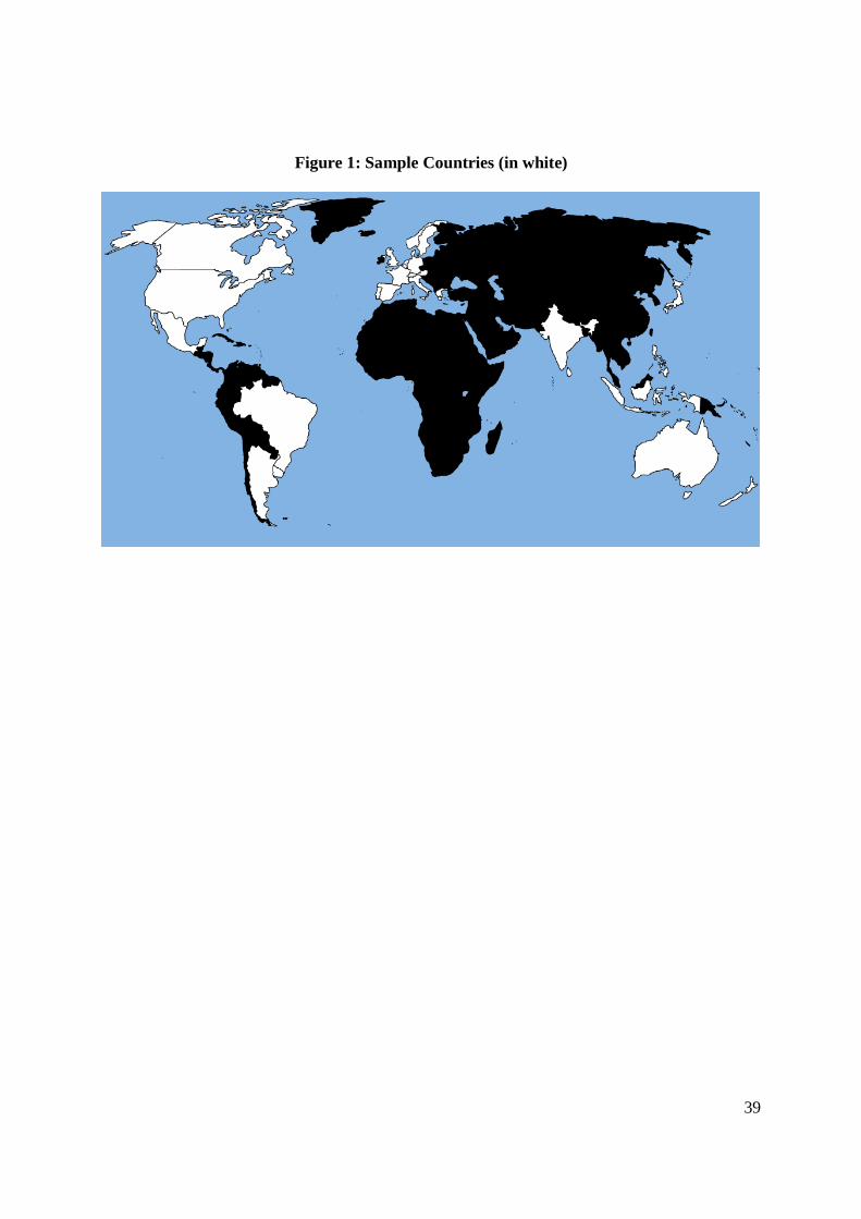
39

Figure 1: Sample Countries (in white)

40

1870-1913 1921-1939 1950-2000N Mean Std. Dev. N Mean Std. Dev. N Mean Std. Dev.

Bilateral trade 11429 18.06 2.23 4940 18.81 1.59 13256 20.45 1.80GDP 11429 20.85 1.74 4940 22.38 1.61 13256 25.13 1.93Distance 11429 8.04 1.19 4940 8.04 1.19 13256 8.04 1.19Exchange rate volatility 11429 0.50 0.50 4940 0.22 0.41 13256 0.08 0.28Common language 11429 0.16 0.37 4940 0.16 0.37 13256 0.16 0.37Imperial membership 11429 0.10 0.30 4940 0.09 0.29 13256 0.09 0.29Shared border 11429 0.12 0.32 4940 0.12 0.32 13256 0.12 0.32

Table 1: Summary Statistics

41

Dependent variable: log of bilateral exports from i to j

Panel A: With country fixed effects

Coefficient Std .Err. Coefficient Std .Err. Coefficient Std .Err.GDP 0.70 0.02 *** 0.82 0.02 *** 0.80 0.01 ***Distance -0.31 0.02 *** -0.15 0.02 *** -0.65 0.01 ***Fixed exchange rate regime 0.45 0.04 *** 0.17 0.03 *** 0.33 0.03 ***Common language 0.48 0.04 *** 0.32 0.05 *** 0.19 0.03 ***Imperial membership 1.66 0.07 *** 0.65 0.08 *** 0.59 0.05 ***Shared border 1.01 0.04 *** 1.00 0.04 *** 0.65 0.02 ***

ObservationsR-squared

Panel B: With country-specific annual fixed effects

Coefficient Std .Err. Coefficient Std .Err. Coefficient Std .Err.GDP - - - - - -Distance -0.38 0.02 *** -0.20 0.03 *** -0.69 0.01 ***Fixed exchange rate regime 0.79 0.06 *** 0.36 0.07 *** 0.64 0.04 ***Common language 0.38 0.05 *** 0.21 0.06 *** 0.19 0.04 ***Imperial membership 1.46 0.08 *** 0.35 0.10 *** 0.33 0.05 ***Shared border 1.09 0.05 *** 1.09 0.06 *** 0.72 0.03 ***

ObservationsR-squared

NB: Country and year fixed effects not reported; robust standard errors; *** significant at the 1% level.

1870-1913 1921-1939 1950-2000

1921-1939 1950-2000

0.6445 0.6243 0.7939

1870-1913

Table 2: Gravity in Three Eras of Globalization

11429 4940 13256

11429 4940 132560.6418 0.6806 0.8380

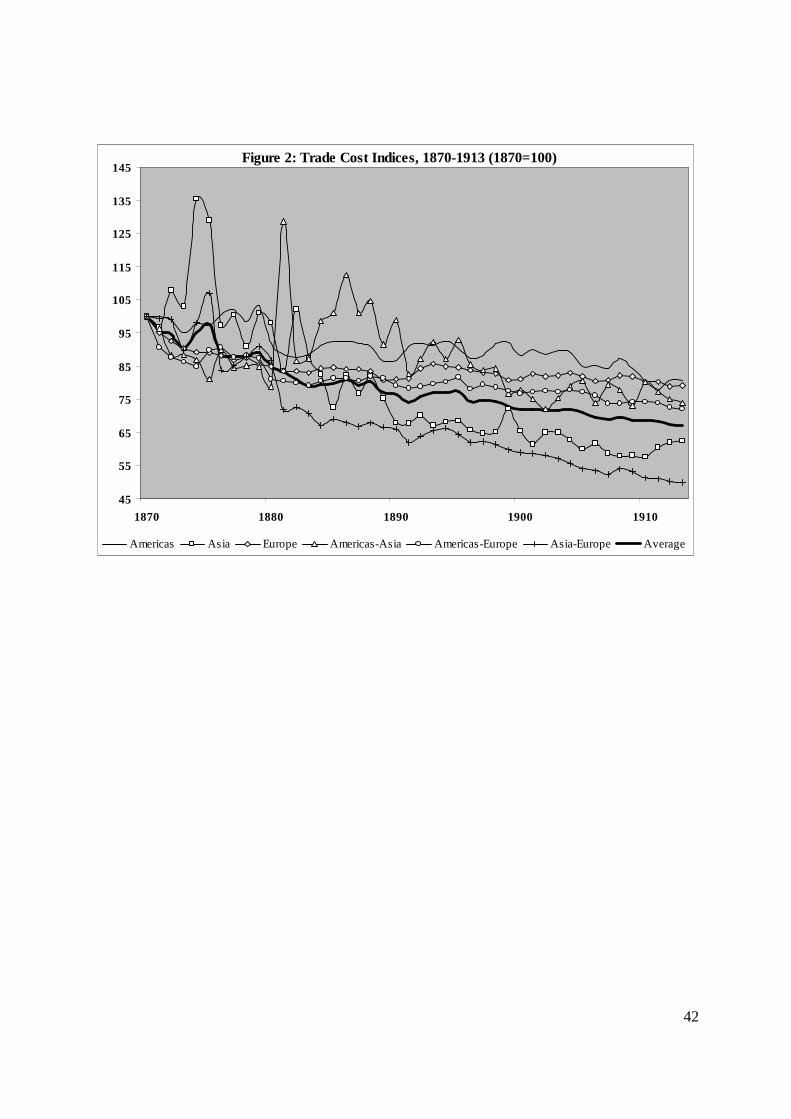
42

Figure 2: Trade Cost Indices, 1870-1913 (1870=100)

45

55

65

75

85

95

105

115

125

135

145

1870 1880 1890 1900 1910

Americas Asia Europe Americas-Asia Americas-Europe Asia-Europe Average

43

Figure 3: Trade Cost Indices, 1921-1939 (1921=100)

45

55

65

75

85

95

105

115

125

135

145

1921 1925 1929 1933 1937

Americas Asia Europe Americas-Asia Americas-Europe Asia-Europe Average

44

Figure 4: Trade Cost Indices, 1950-2000 (1950=100)

45

55

65

75

85

95

105

115

125

135

145

1950 1960 1970 1980 1990 2000

Americas Asia Europe Americas-Asia Americas-Europe Asia-Europe Average

45

Dependent variable: log of bilateral trade costs separating i and j

Coefficient Std .Err. Coefficient Std .Err. Coefficient Std .Err. Coefficient Std .Err.Distance 0.13 0.00 *** 0.11 0.01 *** 0.06 0.01 *** 0.17 0.00 ***Fixed exchange rate regime -0.03 0.01 *** -0.08 0.01 *** -0.04 0.01 *** -0.09 0.01 ***Common language -0.11 0.01 *** -0.14 0.01 *** -0.08 0.01 *** -0.08 0.01 ***Imperial membership -0.28 0.01 *** -0.46 0.02 *** -0.20 0.02 *** -0.15 0.01 ***Shared border -0.26 0.01 *** -0.29 0.01 *** -0.26 0.01 *** -0.22 0.01 ***

ObservationsR-squared

NB: Country and year fixed effects not reported; robust standard errors; *** significant at the 1% level.

0.7251 0.6989 0.8242

Table 3: Determinants of Trade Costs in Three Eras of Globalization

Pooled

148070.6502

1870-1913 1921-1939 1950-2000

5709 2470 6628

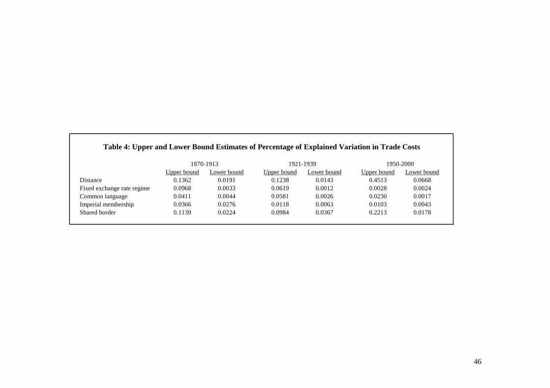
46

Upper bound Lower bound Upper bound Lower bound Upper bound Lower boundDistance 0.1362 0.0191 0.1238 0.0143 0.4513 0.0668Fixed exchange rate regime 0.0968 0.0033 0.0619 0.0012 0.0028 0.0024Common language 0.0411 0.0044 0.0581 0.0026 0.0230 0.0017Imperial membership 0.0366 0.0276 0.0118 0.0063 0.0103 0.0043Shared border 0.1139 0.0224 0.0984 0.0367 0.2213 0.0178

1870-1913 1921-1939 1950-2000

Table 4: Upper and Lower Bound Estimates of Percentage of Explained Variation in Trade Costs

47

Contribution of growth Contribution of growth Contribution of change Contribution of change Average growth of in output in income similarity in trade costs in multilateral factors international trade

(GDP weighted) (GDP weighted) (GDP weighted) (GDP weighted) (GDP weighted)1870-2000 Full sample (n = 130) 744% + -16% + 326% + -25% = 1029%

Americas (n = 6) 886 + 14 + 162 + -1 = 1061Asia/Oceania (n = 7) 610 + 51 + 436 + -24 = 1074Europe (n = 56) 590 + 23 + 330 + -38 = 904Americas-Asia/Oceania (n = 6) 832 + -47 + 511 + -28 = 1268Americas-Europe (n = 35) 808 + -56 + 281 + -22 = 1011Asia/Oceania-Europe (n = 20) 601 + 28 + 386 + -30 = 985

1870-1913 Full sample (n = 130) 225% + -11% + 290% + -18% = 486%

Americas (n = 6) 331 + 0 + 151 + -19 = 463Asia/Oceania (n = 7) 105 + 29 + 434 + -11 = 557Europe (n = 56) 177 + -6 + 176 + -23 = 324Americas-Asia/Oceania (n = 6) 281 + -48 + 339 + -9 = 564Americas-Europe (n = 35) 273 + -26 + 297 + -18 = 524Asia/Oceania-Europe (n = 20) 146 + 20 + 497 + -16 = 647

1921-1939 Full sample (n = 130) 88% + 4% + -87% + -6% = 0%

Americas (n = 6) 82 + 14 + -115 + 9 = -10Asia/Oceania (n = 7) 58 + 12 + -36 + 0 = 34Europe (n = 56) 103 + -2 + -65 + -16 = 20Americas-Asia/Oceania (n = 6) 78 + 6 + -37 + 2 = 48Americas-Europe (n = 35) 86 + 7 + -132 + -6 = -45Asia/Oceania-Europe (n = 20) 85 + 1 + -50 + -6 = 30

1950-2000 Full sample (n = 130) 353% + 8% + 148% + -25% = 484%

Americas (n = 6) 347 + 7 + 16 + -7 = 363Asia (n = 7) 448 + -14 + -27 + -15 = 391Europe (n = 56) 332 + 7 + 331 + -38 = 633Americas-Asia (n = 6) 356 + 29 + 84 + -25 = 444Americas-Europe (n = 35) 343 + 5 + 125 + -23 = 450Asia-Europe (n = 20) 386 + 2 + 185 + -28 = 544

Table 5: Decomposition of Trade Booms and Busts, 1870-2000

48

-60

0

60

120

180

1870s 1880s 1890s 1900s 1910s 1920s 1930s 1940s 1950s 1960s 1970s 1980s 1990s

Figure 5: Trade Growth versus Output Growth (in %)

Trade growth

Output growth